| Issue |
A&A
Volume 706, February 2026
|
|
|---|---|---|
| Article Number | A319 | |
| Number of page(s) | 14 | |
| Section | Extragalactic astronomy | |
| DOI | https://doi.org/10.1051/0004-6361/202557401 | |
| Published online | 17 February 2026 | |
Merger-induced disturbance and temporal signatures in galaxy clusters: A combined phase space and photometric analysis
Department of Physics, Brown University 182 Hope Street Providence RI 02912, USA
★ Corresponding authors: This email address is being protected from spambots. You need JavaScript enabled to view it.
, ian_dell'This email address is being protected from spambots. You need JavaScript enabled to view it.
Received:
24
September
2025
Accepted:
8
January
2026
Abstract
We present a physically interpretable framework to quantify dynamical disturbances in galaxy clusters using projected two-dimensional phase-space information. Based on the TNG-Cluster simulation, we constructed a disturbance score that captures merger-driven asymmetries through features such as velocity dispersion and Gaussian mixture model (GMM) peak fitting, which captures asymmetries indicative of dynamical disturbance. All features were derived from observable quantities and are intended to be measurable in future surveys. To enable observational application, we adopted a simplified estimator using aperture mass map statistics as a mass ratio proxy in TNG300-1, and validated its performance with weak lensing data from The Local Volume Complete Cluster Survey (LoVoCCS). While phase-space diagnostics reveal merger-driven asymmetries, they are not sensitive to whether the secondary progenitor is infalling or receding, and thus cannot distinguish future mergers from past mergers. To address this, we incorporated the star formation rate (SFR) from TNG-Cluster and propose the blue galaxy fraction as a promising observational tracer of merger timing. Finally, we constructed mock Chandra X-ray images of TNG-Cluster halos at redshift z = 0.2, and find that the offset between the X-ray peak and the position of the most massive black hole (used as a proxy for the brightest cluster galaxy) correlates with our disturbance score, serving as a consistency check. We also performed case studies using LoVoCCS observational data, correlating the blue galaxy fraction with disturbance scores derived from the eROSITA morphology catalog.
Key words: gravitational lensing: weak / hydrodynamics / galaxies: photometry / dark matter / X-rays: galaxies: clusters
© The Authors 2026
 Open Access article, published by EDP Sciences, under the terms of the Creative Commons Attribution License (https://creativecommons.org/licenses/by/4.0), which permits unrestricted use, distribution, and reproduction in any medium, provided the original work is properly cited.
This article is published in open access under the Subscribe to Open model. This email address is being protected from spambots. You need JavaScript enabled to view it. to support open access publication.
1. Introduction
Galaxy clusters, the most massive gravitationally bound structures in the universe, serve as critical tracers of structure formation and laboratories for a wide range of astrophysical processes. Cluster mergers, especially major mergers with mass ratios above 0.1 (i.e., where the secondary progenitor contains at least 10% of the mass of the primary), are among the most energetic events in the current universe. These mergers release gravitational energies exceeding 1064 erg, driving shocks and turbulence that heat the intracluster medium (ICM), a diffuse, X-ray–emitting plasma that fills the space between galaxies (Sarazin 2002; van Weeren et al. 2019).
Beyond disturbing the ICM, mergers may also influence the star formation activity of cluster galaxies. However, whether they trigger starbursts or accelerate quenching remains uncertain. Both observations and simulations have reported a wide range of outcomes, including enhanced star formation (e.g., Contreras-Santos et al. 2022; Aldás et al. 2023) and merger-induced quenching (e.g., Deshev et al. 2017; Roberts 2024). Other studies either find no significant global effect beyond localized starbursts (e.g., Rawle et al. 2014), or suggest a two-phase sequence of initial enhancement followed by suppression (e.g., Stroe et al. 2015; Sobral et al. 2015). These mixed results underscore the complexity of merger-driven galaxy evolution.
Despite their astrophysical significance, cluster mergers remain difficult to identify and characterize observationally. A variety of diagnostic tools have been developed, each targeting distinct physical signatures. The common goal is to detect asymmetries and structural disturbances indicative of merger activity. In X-ray imaging, morphological indicators, such as symmetry, peakiness, alignment, concentration, and multipole moments, have been widely used to distinguish dynamically relaxed clusters from disturbed systems (e.g., Mantz et al. 2014; Sanders et al. 2025). The projected offset between the X-ray peak and the position of the brightest cluster galaxy (BCG) is another commonly used proxy, based on the expectation that mergers displace the hot gas relative to the central galaxy (e.g., Jones & Forman 1984; Katayama et al. 2003; Sanderson et al. 2009). Similarly, the offset between the peaks of gravitational lensing mass maps and X-ray emission has also been proposed as an indicator of dynamical disturbance (Poole et al. 2006). The Bullet Cluster (1E 0657-56, Clowe et al. 2006) and its analogs (e.g., Bradač et al. 2008; Bartalucci et al. 2024) provide compelling examples of such separation due to mergers.
More detailed X-ray morphology, such as the presence of cold fronts (e.g., Ghizzardi et al. 2010) and shock edges (e.g., Botteon et al. 2018), can also serve as evidence of merger activity when available. In the radio regime, diffuse synchrotron emission such as radio relics provides complementary signatures of merger-driven shocks and turbulence (e.g., Hlavacek-Larrondo et al. 2018; Golovich et al. 2019; Wilber et al. 2019). These multiwavelength indicators are often combined to improve the robustness of merger identification.
In the optical regime, mergers may appear as multiple peaks in galaxy number density or kinematic substructures in velocity space. Photometric observations can capture spatial asymmetries (e.g., Wen et al. 2024), while spectroscopic measurements, such as those using the Hα line, provide dynamical and star formation information. However, obtaining full-sky, multiwavelength cluster observations remains challenging, making the robust identification of mergers difficult.
While each method offers valuable insight, the identification of merging systems is highly definition-dependent in large observational samples and provides limited information about the timing of merger events. In contrast, cosmological simulations offer full knowledge of each cluster’s merger history, enabling detailed tracking of dynamical evolution and structural disturbance. Many efforts have leveraged simulations to study merger-driven phenomena (e.g., ZuHone et al. 2018; Arendt et al. 2024; Lee et al. 2024), though the use of phase-space distributions, defined by projected positions and line-of-sight velocities, remains relatively uncommon (e.g., van der Jagt et al. 2025). When combined with star formation histories, color evolution, and synthetic observables, such as X-ray morphology or mass maps, such simulation-based approaches offer a powerful testbed for developing generalizable frameworks to trace merger-driven disturbance.
For this work, we aimed to develop a physically interpretable framework for characterizing merger-driven disturbance in galaxy clusters. Using the TNG-Cluster simulation (Nelson et al. 2024), we extracted features from the phase-space distribution of member galaxies and trained a machine learning model to predict a continuous disturbance score. The model was supervised using the true merger history of each cluster, allowing us to construct a score that captures the structural impact of major mergers in a time-sensitive manner.
Since the phase-space machine learning model lacks the ability to distinguish between future and past mergers, corresponding to infalling versus outgoing second progenitors, we further analyzed the evolution of SFR across merger events and examined the blue galaxy fraction as a potential time-sensitive tracer. We find that the disturbance score correlates with both the curvature of star formation histories and the blue fraction in a way that reflects merger timing. As a consistency check, we compared the score with BCG offsets measured from mock X-ray maps.
To connect our framework to observable quantities, we developed a method to estimate mass ratios from aperture mass maps. This estimator was validated using both the TNG300-1 simulation and LoVoCCS observational data (Fu et al. 2022, 2024; Englert et al. 2025a; Fu et al. 2025). We further applied our framework to several LoVoCCS clusters as case studies.
This paper is organized as follows. In Section 2, we describe the simulations and methodology. Section 3 presents the machine learning model, the evolution of star formation rate (SFR), the behavior of blue galaxy fractions, the correlation between BCG offsets and our disturbance score, and our aperture mass ratio estimator. In Section 4, we discuss the grouping strategy for model training, the impact of projection choices, efforts to mitigate richness dependence, and case studies applying our method to LoVoCCS clusters. We summarize our conclusions in Section 5.
2. Data and methods
2.1. The TNG-Cluster simulation
TNG-Cluster (Nelson et al. 2024) is a spin-off project of the IllustrisTNG suite (Nelson et al. 2019), with particular emphasis on high-mass clusters beyond those captured in TNG300. To improve statistics for massive systems, the parent box of TNG-Cluster is significantly larger than that of TNG300, reaching up to 1 Gpc, and includes 352 high-mass clusters (> 1014 M⊙) via zoom-in simulations. The zoom-in regions feature resolutions comparable to TNG300-1, with a dark matter particle mass of 6.1 × 10⁷ M⊙ and a mean baryonic cell mass of 1.2 × 10⁷ M⊙.
We used the 352 primary zoom-in halo targets in TNG-Cluster, along with their main progenitors, as our main sample. We traced them from snapshots 72 to 99, ranging from redshift 0.4 to 0, extracted features from their phase-space information, and tracked the evolution of their SFR and blue galaxy fraction. We also generated mock X-ray images at redshift 0.2. Further details are provided in the following sections.
2.2. The TNG300-1 simulation
In addition to the limited number of samples with large mass ratios, we also utilized data from TNG300-1. TNG300-1 is part of the IllustrisTNG suite and has been introduced in a series of papers (Nelson et al. 2019; Pillepich et al. 2018; Nelson et al. 2018; Naiman et al. 2018; Marinacci et al. 2018). In TNG300-1, the dark matter particle mass is 0.9 × 10⁷ M⊙, and the mean baryonic cell mass is 1.1 × 10⁷ M⊙.
We focused on halos more massive than 1013 M⊙ at redshift 0.08 to validate our rapid method for estimating the mass ratio. In both TNG-Cluster and TNG300-1 analyses, we adopted the same cosmological parameters used throughout the TNG simulations, consistent with the Planck 2015 results (Planck Collaboration XIII 2016): ΩΛ, 0 = 0.6925, Ωm, 0 = 0.3075, Ωb, 0 = 0.0486, σ8 = 0.8159, ns = 0.9667, and h = 0.6774. These values are defined within the astropy.cosmology module (Astropy Collaboration 2022; Planck Collaboration XIII 2016).
2.3. LoVoCCS data
The Local Volume Complete Cluster Survey (LoVoCCS) is an ongoing program aiming to observe nearly one hundred low-redshift, X-ray–luminous galaxy clusters using the Dark Energy Camera (DECam). Aperture mass maps and weak-lensing–based mass estimates for a subset of these clusters have already been produced through the LoVoCCS pipelines, as described in a series of papers (Fu et al. 2022, 2024; Englert et al. 2025a,b).
We performed the proxy analysis with clusters covered by Fu et al. (2024). This serves as an initial attempt to connect our simulation-based framework to observational data across six bands (u, n, g, r, i, z), where we made use of u- and g-band photometry.
2.4. Phase-space feature extraction
We extracted all subhalos associated with the 352 zoom-in targets using the group catalogs of the TNG-Cluster simulation. To define the projected radius on the 2D plane perpendicular to the line of sight, we first computed the projected positions (xn, yn) of all subhalos and subtracted their mean position  . From these centered coordinates we constructed the 2 × 2 covariance matrix:
 (1)
(1)
where xn is the position vector of each subhalo, and μ is their mean position. We then performed a principal component analysis (PCA) of C using scikit-learn (Pedregosa et al. 2011). The eigenvectors of C give two orthogonal directions of maximum and minimum variance of the subhalo distribution, and the corresponding eigenvalues give the variance (squared dispersion) along these directions. The eigenvector associated with the largest eigenvalue defines the projected major axis of the halo; we rotated the coordinate system so that this axis lay along the x–direction and defined the projected radius of each subhalo as its coordinate along this axis. For velocity, we retained only the component along the line of sight, perpendicular to the projected plane, consistent with what is accessible in real observations. We further used the same covariance matrix C to characterize the projected halo shape. Its eigenvalues λ1 ≥ λ2 represent the variance along the major and minor principal axes, and their ratio λ2/λ1 provides a measure of the minor-to-major axis ratio.
To further characterize the phase-space structure, we fitted Gaussian mixture models (GMMs) using scikit-learn (Pedregosa et al. 2011) to the projected radius–velocity distribution of all subhalos associated with each halo. From the best-fitting models, we extracted features such as the mean projected radius, mean line-of-sight velocity, and the subhalo count of each component. We also recorded the maximized likelihoods of the K-component fits (K = 1, 2) and used them to compute the Bayesian information criterion (BIC; Schwarz 1978):
 (2)
(2)
where  is the maximum likelihood of the best-fit K-component model, N is the number of members used in the fit, and kK is the number of free parameters.
In addition, we included the mass ratio between the central subhalo and the most massive satellite galaxy within each friends-of-friends (FOF) halo, as identified by the group catalogs.
Our final dataset includes the 352 primary zoom-in halos and their main progenitors from redshift z = 0.4 to z = 0, corresponding to snapshots 72 to 99. For each halo, we extracted phase-space information along all three Cartesian projections. To increase the number of training samples, we treated each projection as an independent input. To avoid data leakage, we tested different grouping strategies, which are further discussed in the results and discussion sections.
2.5. Merger score definition
We define the merger score as a time-weighted cumulative contribution from all major merger events associated with a given halo, using an exponentially decaying function of their time separation from the current snapshot:
 (3)
(3)
where Δt is the time interval between the current snapshot and the merger event, and τ is a characteristic decay timescale. Recent mergers (small Δt) contribute more significantly, while earlier events are exponentially suppressed.
To probe dynamical states across time, we define three versions of the score: the past-merger score, computed by summing only mergers that occurred before the current snapshot; the future-merger score, based on mergers that will occur after it; and the full-merger score, which includes all merger events and equals the sum of the past and future scores when evaluated using the same decay timescale τ.
We considered only major mergers, defined as interactions between a primary halo (i.e., one of the 352 TNG-Cluster zoom-in targets with M500c > 1014 M⊙ at redshift 0) and a secondary halo with Mhalo > 1013 M⊙. Halo masses were taken from the Group_M_Crit500 field in the TNG-Cluster group catalogs, corresponding to the mass enclosed within a sphere whose mean density is 500 times the critical density of the universe at the redshift of the halo. Merger information was obtained from the catalog of Lee et al. (2024).
2.6. Star formation and blue galaxy fraction statistics
We traced the 352 primary zoom-in halos in TNG-Cluster along their main progenitor branches back to redshift 0.4, using the group catalogs to identify their member galaxies. For each FOF halo, we calculated the average star formation rate (SFR) of its member subhalos. To capture merger-induced SFR variations, we analyzed SFR evolution within a fixed symmetric 2 Gyr time window centered on each snapshot (1 Gyr before and 1 Gyr after; see Section 3.2 for details). Specifically, we normalized the SFR of a given halo at a particular snapshot by the average SFR of that halo over this surrounding time window.
To quantify the time evolution, we computed the curvature of the normalized SFR history using the following estimator:
 (4)
(4)
To estimate the blue galaxy fraction in each FOF halo, we extracted absolute magnitudes from the SubhaloStellarPhotometrics field in the group catalogs. Apparent magnitudes are computed based on redshift. To avoid the regime where observational band errors become substantial, we imposed a magnitude cut at u, g < 23, 25, and applied the same cut to the simulations for consistency. We define galaxies as “blue” if their u − g color is less than or equal to 0.3. We adopt this relatively strict color cut to avoid overestimating the blue fraction at redshifts near 0, where fainter member galaxies can enter the sample due to the apparent magnitude cut.
2.7. X-ray image generation
We selected the progenitors of the 352 primary zoom-in halos from TNG-Cluster at redshift z = 0.2 (snapshot 84) and downloaded their cutout files, which contain only the high-resolution particles associated with these halos. We adopted z = 0.2 as our reference redshift for practical reasons: the hot gas can be identified using the GFM_CoolingRate field, which is only stored at a small set of snapshots in TNG-Cluster (e.g., z = 0.0, 0.1, 0.2, 0.3), and the merger trees at z = 0.2 still provide a long enough future time span (≳1 Gyr after this snapshot) to track mergers for our choice of τ = 1 Gyr in the merger scores.
X-ray photon maps were generated using pyXSIM (ZuHone & Hallman 2016) and SOXS (ZuHone et al. 2023), with the instrument configuration set to chandra_acisi_cy22, assuming an exposure time of 2000 ks and an effective collecting area of 600 cm2. The Chandra ACIS-I array has a field of view of 16.9 × 16.9 arcmin. In SOXS, the chandra_acisi_cy22 configuration corresponds to a square field of view of ≃20.008 arcmin; this slightly larger nominal FoV only affects the empty outer regions of the synthetic images and has no impact on our BCG-offset measurements, which lie well within the ACIS-I array. The simulated X-ray images were produced in the soft band, restricting photon energies to 0.1–2.0 keV.
We centered the images on the group positions of each halo and generated X-ray photons within a cubic region of side length 2× Group_R_Crit500. To locate the brightest X-ray peaks, we smoothed the photon maps with a Gaussian kernel, achieving a final resolution of approximately 10 kpc. Following Prunier et al. (2024), we define the BCG offset as the projected distance between the brightest X-ray pixel and the position of the most massive black hole within the corresponding FOF halo. Fig. 1 shows the X-ray images of FOF halo 0, for which Group_R_Crit500 is 1474 kpc.
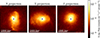 |
Fig. 1. Mock X-ray images of FOF halo 0 from three projections (X, Y, and Z), centered on the group position and smoothed to a ∼10 kpc resolution. Black dots mark the centers used for cropping. A 1000 kpc scale bar is shown in each panel. The color indicates the photon counts, normalized using logarithmic scaling. |
2.8. Aperture mass maps simulation
We developed a fast method for estimating mass ratios using aperture mass maps, validated on both TNG300-1 and LoVoCCS data. In TNG300-1, we selected halos at redshift z = 0.08 (snapshot 92), chosen to match the typical redshift of the LoVoCCS cluster sample. Our sample includes halos with M200c > 5 × 10¹³ M⊙ and halos with 1013 M⊙ < M200c < 5 × 10¹³ M⊙ that have mass ratios greater than 0.1. Here, M200c is defined by the Group_M_Crit200 field in the group catalogs as the mass enclosed within a sphere whose mean density is 200 times the critical density of the universe at the halo redshift. Particles within R200c were extracted and projected along the z-axis to generate surface density maps. The projection depth along the line of sight was set to 4 × R200c.
To simulate the aperture mass signal-to-noise (S/N) map, we began with the convergence κ(θ). After converting κ(θ) to the shear γ(θ), we combined the resulting shear field with the intrinsic ellipticities of galaxies to generate mock observed ellipticities. The aperture mass maps were then constructed following the LoVoCCS pipeline (Fu et al. 2024).
The convergence is defined as the dimensionless surface mass density:
 (5)
(5)
Here Σcr, Dd, Ds, and Dds denote the critical density, the angular diameter distances to the lens, to the source, and from the lens to the source, respectively. In our setup, the lens (i.e., the target FOF halos) was placed at redshift 0.08, and the source (i.e., background) was assumed to lie at redshift 1.0.
The Fourier transform of the convergence field κ(θ) is defined as
 (6)
(6)
Following Bartelmann & Schneider (2001), the shear in Fourier space is related to the convergence via
 (7)
(7)
with the kernel
 (8)
(8)
The resulting shear field is then transformed back to real space.
We assumed a background galaxy number density of 20 arcmin−2 and an intrinsic shape noise of σϵ = 0.3, according to The LSST Dark Energy Science Collaboration (2018), noting that the morphology of S/N maps is not strongly sensitive to the choice of σϵ. Background galaxies were randomly distributed, and their observed ellipticities were calculated from the shear γ(θ) and the convergence κ(θ). In the weak lensing limit, where κ ≪ 1, γ ≪ 1, the observed ellipticity ϵ can be modeled as
 (9)
(9)
where
 (10)
(10)
Here, ϵgal denotes the intrinsic (unlensed) ellipticities of galaxies. A full derivation is provided in Bartelmann & Schneider (2001).
Based on the observed ellipticities, we computed aperture mass statistics following the LoVoCCS pipeline (Fu et al. 2022), applying the Schirmer filter (Schirmer 2004; Schirmer et al. 2004; Hetterscheidt et al. 2005) as the weighting function Q to integrate the tangential shear in Eq. (11), to match the weighting function used in LoVoCCS, where x = R/Rap with Rap the aperture radius.
The resulting aperture mass S/N map was computed using Equation (12), with Q as the Schirmer filter, |ϵ| as the modulus of the complex ellipticity, ϵi the tangential component of the member galaxy ellipticity serving as an estimator of the tangential shear γt in the weak-lensing limit, and the summation taken over galaxies within the aperture radius:
 (11)
(11)
 (12)
(12)
As halos in TNG300-1 are less massive than LoVoCCS clusters, to enhance the signal-to-noise ratio for low-mass halos, we scaled the background galaxy density by a factor of (Mhalo/5 × 1014 M⊙)2, where 5 × 10¹⁴ M⊙ is approximately the median mass of the LoVoCCS clusters. We define the mass ratio of each FOF halo as the mass of the most massive satellite subhalo (within the region used to generate the aperture mass maps) divided by the mass of the central subhalo. Fig. 2 shows an example of our mock observations for FOF halo 142 in the TNG300-1 simulation.
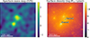 |
Fig. 2. Example mock observation from the TNG300-1 simulation. A 500 kpc scale bar is shown in each panel. Left: Simulated aperture mass map (S/N) of FOF halo 142, with R200c ∼ 750kpc, incorporating shape noise consistent with observational weak lensing data. For visualization, the maps are Gaussian-smoothed with a kernel scale of ∼60 kpc; this smoothing is applied for display purposes only. Right: Surface mass density map (dark matter + gas) in units of log M⊙/pixel. The positions of the central and the most massive satellite subhalos are marked for reference. |
2.9. Mass ratio estimation
We used the peak_local_max function from scikit-image (van der Walt et al. 2014) to identify the brightest peaks in the aperture mass maps generated from both TNG300-1 and LoVoCCS clusters. Each map covers a field of view of 2R200 on a side and is discretized on a 240 × 240 grid, corresponding to a pixel size of Δx = (2R200)/240 = R200/120 in physical units. After applying a ten-pixel Gaussian smoothing, the two highest peaks were assumed to correspond to the central and the most massive satellite subhalos. We then constructed an empirical quantity, defined in Equation (13), by taking the ratio of their peak intensities and multiplying it by their separation distance. By correlating this constructed quantity with the true mass ratios, we aimed to establish a proxy that can be applied to observations with known mass ratios.
In the TNG300-1 simulation, the true mass ratio is defined as the ratio of the SubhaloMass values in the group catalog, which represents the total bound mass of each subhalo. In the LoVoCCS clusters, we estimated the mass ratio using weak lensing reconstruction pipelines, under the assumption that the two peaks correspond to two distinct cluster centers.
The empirical quantity q is defined via
 (13)
(13)
where I1 and I2 are the intensities of the first and second brightest peaks in the aperture mass map, and Rsep is their projected separation on the map. In practice, we measured Rsep in pixel units on the 240 × 240 grid; the corresponding physical separation is Rsep Δx, where Δx = (2R200)/240 is the map pixel size. Since I2/I1 is dimensionless, q has the same units as Rsep. We note that this empirical proxy may be sensitive to the choice of smoothing kernel and the relative sizes of the cluster and its subhalos. In particular, an overly small kernel may underestimate the peak intensity of extended subhalos, while a large kernel can smear out more compact structures. The optimal kernel size is nontrivial to determine and may vary across systems; in this work, we adopted a fixed value because our aim was to demonstrate correlation rather than optimize the mass fraction measurement.
3. Results
3.1. Phase-space disturbance
3.1.1. Decay timescale selection
To quantify the connection between dynamical disturbance and merger history, we first determined a proper decay timescale τ in the merger score definition (Eq. (3)). This parameter controls how strongly recent mergers contribute relative to older ones. For this pre-evaluation, we included all candidate features and pruned them after selecting a suitable τ. We evaluated the model performance based on R2 in the training and test datasets. Here R2 denotes the standard coefficient of determination computed between the true disturbance scores si and the predicted scores  and is defined via
 (14)
(14)
where  is the mean of the true scores. Thus, R2 = 1 corresponds to a perfect prediction, R2 = 0 indicates performance no better than predicting the mean, and negative values imply worse-than-baseline performance.
The choice of τ is guided by two considerations. First, we evaluated model performance by training XGBoost (Chen & Guestrin 2016), via scikit-learn (Pedregosa et al. 2011) to predict full-, past-, and future-merger scores from all phase-space features, and tracking how the test R2 varies with τ. Second, we accounted for sample availability: halos within τ Gyr of redshift 0 lack complete future-merger information and must be excluded when using full- or future-merger scores. Increasing τ enlarges this exclusion window and reduces the effective sample size. XGBoost, a scalable tree boosting system, was chosen for its ability to capture nonlinear relationships and its interpretability via feature-importance metrics.
To increase both sample size and model robustness, we treated the three projections of each of the 352 primary zoom-in targets and their progenitors between snapshots 72 and 99 as distinct samples. When splitting the dataset into training and test sets, we used grouping: we assigned each sample a group label and performed the split at the level of group labels, i.e., all samples sharing the same label were placed entirely in either the training set or the test set. However, the degree of data leakage can depend on the chosen grouping scheme. Grouping by both halo ID and snapshot number can prevent leakage between different projections of the same halo at the same snapshot, but it still allows different snapshots of the same halo to fall into different splits and can therefore introduce temporal leakage since adjacent snapshots are strongly correlated, for example, the model might learn to predict the merger score at snapshot 73 by implicitly memorizing the features of the same halo at snapshot 72.
To mitigate this, we applied a projection-rotation scheme along with snapshot dropping. Specifically, we alternated between using different phase-space projections (x, y, and z) and excluded the snapshots in between. For example, in the sequence [z, drop, x, drop, y, drop], each included snapshot has a distinct projection and is separated from its adjacent neighbors. This setup helps reduce the risk of data leakage by discouraging the model from learning patterns that depend on the similarity of halo structures across consecutive snapshots, which may act as a proxy for halo identity.
To assess potential data leakage, we conducted two complementary tests. First, we experimented with a more conservative grouping strategy where we split data only by halo ID, without including snapshot information. This setup leads to a slightly lower test R2 ∼ 0.40 and training R2 ∼ 0.70 for past-merger scores at τ = 2.0 Gyr, as described in 4.1, compared to the results grouped by both halo ID and snapshot number (Rtest2 ∼ 0.55, Rtrain2 ∼ 0.80). This comparison raises concern about possible data leakage when grouping by both halo ID and snapshot number. To further test for potential data leakage, we constructed a dedicated test set by randomly selecting 20% of halos and excluding them entirely from the training process. We then applied the same training configuration as in the main analysis, including projection-rotation and grouping by both halo ID and snapshot, and evaluated model performance on both the internal test split and the pre-separated test sets. The model achieves consistent scores across both sets. These two additional tests might imply that our projection-rotation scheme and grouping strategy do not lead to severe data leakage while increasing sample diversity.
We note that the snapshots are spaced in redshift rather than in equal time intervals, so halos near redshift 0.4 are separated by shorter physical times. As a result, their structural properties change little across snapshots, increasing the risk that the model learns to associate nearly identical halos across time steps rather than extracting generalizable features. Furthermore, for large values of τ, merger scores become more similar across nearby snapshots, raising the chance that the model relies on learning from a halo’s immediate progenitors or descendants.
We performed a grid search for each τ, using learning rates in {0.005, 0.01, 0.05, 0.1, 0.2}, maximum tree depths in {1, 2, 4, 6, 8, 10}, and numbers of estimators in {100, 200, 300, 500, 1000}. Each model was trained with its own optimized hyperparameters under this scheme, and the resulting performance was used to compare across different τ values. The scan results are shown in Fig. 3.
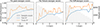 |
Fig. 3. Model performance as a function of τ, evaluated using three target score definitions: past-merger (left), future-merger (middle), and full-merger (right) scores. Orange lines show the R2 on the training set, and blue lines show the R2 on the test set. All results are based on the rotated projection configuration described in Section 3.1.1. |
Considering both the limited sample size and the risk of data leakage, we adopted a small value of τ = 2.0 Gyr, at which the training and test R2 curves begin to stabilize. To ensure a fair comparison across the three merger score definitions, we matched their time windows: the future- and past-merger scores were computed over a window of τ, while the full-merger score used a symmetric window of τ/2 before and after the snapshot. As shown in Fig. 3.1.1, the model trained on past-merger scores performs slightly better. However, this advantage may be partly due to sample loss in the other two definitions at larger τ. Overall, the differences in model performance are minor, suggesting that our phase-space features alone are not sufficient to distinguish between different merger stages. The input features are summarized in the right panel of Fig. 4. We define Δbic as bic2 − bic1 − 6ln(n), which is independent of n, the number of member galaxies. To see why this definition is independent of richness, recall that for a K-component 2D GMM, BIC can be computed via Eq. 2. For our 2D GMMs, k1 = 5 and k2 = 11, hence Δbic ≡ (bic2 − bic1)−6lnN removes the explicit lnN term and is therefore independent of richness. The method for calculating λ2/λ1 is described in Section 2.4.
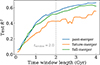 |
Fig. 4. Test R2 as a function of the time window length for the past-, future-, and full-merger scores. The right panel summarizes the phase-space input features used in the model. |
3.1.2. Model performance at selected τ
We evaluated permutation feature importance for models trained on the three merger score definitions, using a time window of 2.0 Gyr. Specifically, this corresponds to τ = 2.0 Gyr for the past- and future-merger scores, and a symmetric window of τ = 1.0 Gyr for the full-merger score. Permutation feature importances for all features are presented in Fig. 5, and we retained only those with a relative importance greater than 0.01 in at least one of the three models. The resulting set includes Δv, σr, 1, σr, 2, σv, 2, bic1, bic2, Δbic, λ2/λ1, z, fm, σr, and σv. Although σv, 1 does not meet the > 0.01 criterion, we added it to the pruned feature set for symmetry, given that σv, 2 is retained and the grouping depends on the adopted GMM fitting method. Fig. 6 presents scatter plots of the predicted versus true scores for all three models trained on the pruned feature set, while Fig. 7 shows the corresponding score distributions.
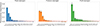 |
Fig. 5. Comparison of permutation feature importance rankings for models using the three merger score definitions: past-merger (left), future-merger (middle), and full-merger (right) scores. Bars indicate the mean importance of each feature, with error bars representing the standard deviation over 10 independent permutations. The red dashed line marks the 0.01 threshold used for feature selection. Features are labeled F1–F17, ranked by importance within each model. Their definitions are as follows: F1: ΔR, F2: v1, F3: v2, F4: Δv, F5: σr, 1, F6: σr, 2, F7: σv, 1, F8: σv, 2, F9: fn, F10: bic1, F11: bic2, F12: Δbic, F13: λ2/λ1, F14: z, F15: fm, F16: σr, F17: σv. |
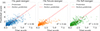 |
Fig. 6. Predicted merger scores versus true scores for three test sets: on past-merger (left), future-merger (middle), and full-merger (right) scores. The red dashed line indicates the ideal case of perfect prediction. Each panel also displays the R2 score for the corresponding test. Points are slightly transparent to indicate density. The model shows consistent predictive performance across different temporal subsets. High true scores tend to be underpredicted. This is mainly because the strongly skewed true-score distribution (Fig. 7): most halos have low scores, which dominate the training and bias the predictions toward low values. |
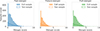 |
Fig. 7. Distribution of true merger scores for the full sample (filled bars) and the test sample (outlined bars), shown for the past-merger, future-merger, and full-merger datasets. |
3.2. Photometric differentiation of merger stages
To investigate whether photometric features can differentiate past from future mergers, we compared results using the past- and future-merger scores defined in Section 2.5. We selected 352 primary zoom-in targets for snapshots between redshift 0.4 and 0 (corresponding to snapshot 72 to 99), treating each snapshot of a halo as an independent sample.
We adopted a time window of 2.0 Gyr to track the evolution of the SFR, measuring it from 1 Gyr before to 1 Gyr after each snapshot. To ensure reliable curvature estimates, we discarded SFR tracks with fewer than three time points, which typically arises from limited redshift resolution or from the restricted redshift range of the analysis. While 2.0 Gyr is somewhat longer than the characteristic timescale of major merger events, a shorter window would reduce the number of available samples due to resolution limits and lead to larger uncertainties. We also tested a shorter window of 1.0 Gyr and found that the results remain consistent.
For correlations involving the future-merger score, we further excluded samples within 2.0 Gyr of redshift 0, where future merger activity cannot be reliably traced. The curvature of normalized SFR is computed as described in Section 2.6.
As shown in Fig. 8, the correlations between SFR curvature and merger scores exhibit distinct trends for past and future mergers.
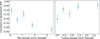 |
Fig. 8. Curvature of the normalized SFR as a function of merger score. The left and right panels show results for the past- and future-merger scores, respectively. In each case, the score distribution is divided into five quantile bins. A total of 9812 samples are used in the past-merger analysis and 5609 in the future-merger case. Error bars indicate the standard error of the mean curvature within each bin. |
Motivated by the SFR results, we investigated whether a directly observable quantity can serve as a proxy for distinguishing between the two merger scores, a task for which phase-space-based machine learning methods have shown limited success, as shown in Section 3.1.1. We computed the blue galaxy fraction as described in Section 2.6, and excluded samples below redshift 0.15 in the future-merger analysis to ensure sufficient look-forward time. As shown in Fig. 9, the trends differ noticeably between the two cases, suggesting that the blue galaxy fraction may carry physical information relevant to merger stages.
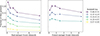 |
Fig. 9. Fraction of blue galaxies as a function of merger score, shown separately for past-merger scores (left) and future-merger scores (right). Each curve corresponds to a redshift bin defined as [zlow, zhigh), i.e., including the lower bound but excluding the upper bound. Within each redshift bin, the score distribution is divided into five quantile bins. Error bars indicate the standard error of the mean blue fraction within each merger score bin. Several redshift bins are absent in the future-merger panel due to the exclusion of low-redshift samples (z < 0.15). |
3.3. BCG offset as a morphological merger indicator
We excluded a small number of clusters with BCG offsets exceeding 500 kpc, as such large displacements are not detectable in observations and primarily result from definitional artifacts in the simulation. Specifically, our BCG offset is defined as the distance between the X-ray peak and the most massive black hole, which can reside in different progenitors during major mergers.
As shown in Fig. 10, the BCG offset measured along the x-projection shows a strong positive correlation with the past-merger score, suggesting that our catalog-based merger scores are consistent with traditional dynamical disturbance indicators. Notably, BCG offsets are more sensitive to past mergers than to upcoming ones, revealing a time asymmetry that phase-space features do not capture. To ensure a fair comparison across different merger score definitions, we adopted matched time windows: τ = 2.0 Gyr for both the past- and future-merger scores, and a symmetric window of τ = 1.0 Gyr for the full-merger score.
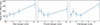 |
Fig. 10. Mean BCG offset as a function of merger score under three definitions: past-merger (left), future-merger (middle), and full-merger (right) scores. Each point represents the average offset within a merger score bin, with vertical bars indicating the standard error of the mean. The total sample size is 325 clusters. To ensure roughly equal sample counts in each bin, we apply quantile-based binning: full- and past-merger scores are divided at [0.0, 0.2, 0.4, 0.6, 0.8, 1.0]; future-merger scores are divided at [0.0, 0.3, 0.48, 0.66, 0.84, 1.0] due to the heavy concentration near zero. A clear positive trend is visible in the first panel, suggesting that BCG displacement increases with merger activity based on past events. |
Since BCG offsets measured along different projection axes are highly correlated, with Pearson correlation coefficients of r = 0.85, 0.89, and 0.83 for the xy, xz, and yz projection pairs, respectively, we used only the x-projection in our analysis.
3.4. Mass ratio estimation
We validated our mass ratio estimator using the LoVoCCS cluster sample by correlating the derived peak intensity ratio (see Eq. (13)) with the true mass ratios. The true mass ratio was inferred from the global two–component weak–lensing mass model: we assumed that the two subclusters are located at the brightest and second–brightest peaks in the aperture–mass map, and we used the LoVoCCS mass–fitting pipeline to derive the masses of these two components, as described in McCleary et al. (2015). The ratio of these fitted masses was used as the true mass ratio for the observed clusters. After excluding halos with identified mass ratios greater than one, caused by incorrect peak identification (e.g., misidentification of the central or secondary subhalos), we find a Pearson correlation coefficient of r = 0.31.
We further tested the estimator with TNG300-1 halos, selecting those with M200c > 5 × 10¹³ M⊙ as well as halos with 1013 M⊙ < M200c < 5 × 10¹³ M⊙ that have true mass ratios above 0.1. Applying the same method using a 10-pixel Gaussian smoothing scale on the aperture mass maps (240 × 240 pixels), consistent with the LoVoCCS setup, yields a Pearson correlation coefficient of r = 0.49. Results for both LoVoCCS and TNG300-1 are shown in Fig. 11. In Fig. 11, the mass ratios in the LoVoCCS clusters are typically larger than those in TNG300-1. This likely reflects a difference in how the mass ratio is defined. In TNG300-1 we are looking at the scale of a single host cluster, so the mass ratio is defined as that between the most massive satellite galaxy and the central subhalo. In LoVoCCS, however, the field of view is typically larger, so the fitted masses can instead correspond to two nearby cluster-scale halos. This difference does not strongly affect our main goal, which is to build a mass-ratio estimator based on aperture-mass maps of two dominant matter clumps, regardless of whether they correspond to a cluster–subcluster pair or to two neighboring clusters. The relatively low correlation coefficient between the true mass ratio and our estimator is expected for several reasons. First, most of the clusters in our sample have small mass ratios (e.g., ≤0.3), so that even modest observational noise or peak–finding uncertainties translate into large relative errors on the inferred ratio. Second, our estimator is based on identifying and measuring the two brightest peaks in the aperture–mass map. Small misidentifications (e.g., confusing a noise peak) or small shifts in the peak position can significantly change the measured peak ratio. For these reasons we do not expect q to be a precise mass–ratio estimator, but rather a coarse indicator that is primarily useful when combined with other features in the classifier.
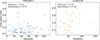 |
Fig. 11. Correlation between the quantity, i.e., q in Equation 13, and the true merger mass ratio. Left: Results from TNG300-1 halos. Right: LoVoCCS observed clusters. Each point represents a galaxy cluster; the x-axis shows the quantity estimator defined in Eq. (13), and the y-axis shows the true mass ratio. We report both Pearson r and Spearman ρ correlation coefficients to characterize the relationship. |
4. Discussion
4.1. Data leakage-minimized baseline
To avoid potential data leakage, we adopted a conservative train-test splitting strategy: for each halo in the training set, none of its progenitors or descendants were included in the test set. This ensures that the model cannot learn merger scores through evolutionary connections. For this evaluation, we used a consistent set of halos selected using the rotation-based filtering scheme described in Section 3.1.1. Models were trained on all candidate features (Fig. 3.1.1) for each of the three merger score definitions, and we scanned across values of τ. The hyperparameters were kept consistent with those used in Section 3.1.1. As shown in Fig. 12, the train and test R2 curves do not differ significantly from those in Fig. 3, suggesting that no strong data leakage is present.
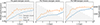 |
Fig. 12. Model performance as a function of τ, evaluated using three target score definitions: past-merger (left), future-merger (middle), and full-merger (right) scores. Orange and blue curves show the training and test R2, respectively, and gray histograms indicate the sample count. This test uses the leakage-minimized split (grouping by halo ID only, so that progenitors and descendants of training halos are excluded from the test set) together with the rotation-based filtering scheme for sample selection. |
4.2. Projection robustness
To assess whether additional information can be extracted from the three projections of each FOF halo, we tracked 352 primary zoom-in targets from redshift 0.4 to 0 and treated the three projections of each halo as independent samples. To minimize data leakage, we applied the same grouping strategy as in Section 4.1, grouping by halo ID when splitting the training and test sets. The model was trained using all candidate features listed in Fig. 4, and we scanned across different values of τ for all three merger score definitions, as shown in Fig. 13. The performance does not show significant improvements, which might imply that the phase-space diagram generated from a single projection is enough to carry the information we need statistically.
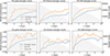 |
Fig. 13. Model performance as a function of τ, evaluated using three target-score definitions: past-merger (left), future-merger (middle), and full-merger (right) scores. Orange and blue curves show the training and test R2, respectively, and gray histograms indicate the sample count. These tests assess projection robustness. Top: Treating the three orthogonal projections of each halo as independent samples, using the leakage-minimized split (grouping by halo ID). Bottom: Following the setup in Section 3.1.1 (grouping by halo ID and snapshot number and using rotation-based filtering), the projection-rotation order is changed from [z, drop, x, drop, y, drop] to [x, drop, y, drop, z, drop]. The similar performance suggests that the model is not sensitive to the projection order, which is favorable for observational applications where only one projection is available. |
We further tested the robustness of our phase-space machine learning model by changing the rotation sequence of projections. While still following the [axis, drop, axis, drop, axis, drop] pattern described in Section 3.1.1, we switched the order from the original [z, drop, x, drop, y, drop] to [x, drop, y, drop, z, drop]. The model was trained on all candidate features listed in Fig. 3.1.1, and we scanned over values of τ for each merger score definition, as shown in Fig. 13. The resulting R2 curves remain stable, suggesting that the model performance is not sensitive to the choice of projection sequence, a reassuring result, as only one projection is actually observable for real clusters.
4.3. Construction of richness-independent features
Since not all galaxy members can be reliably identified in observations, we constructed a model that minimized dependence on richness. Following the same procedures as in Section 3.1.1, we trained the model using the following features: Δv, σr, 1, σr, 2, σv, 1, σv, 2, Δbic, λ2/λ1, z, fm, σr, and σv. These features are designed to be explicitly independent of the number of member subhalos.
Figs. 14 to 15 present the model results under this feature set. Specifically, we show the τ-scan results for all three merger score definitions, scatter plots of predicted versus true scores at τ = 2.0 Gyr for past- and future-merger scores and τ = 1.0 Gyr for full-merger score, as well as the corresponding feature importances. The test R2 slightly decreases compared to the full-feature models (which include bic1 and bic2), but overall performance remains acceptable and interpretable.
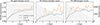 |
Fig. 14. Model performance as a function of τ, evaluated using three target-score definitions: past-merger (left), future-merger (middle), and full-merger (right) scores. Orange and blue curves show the training and test R2, respectively, and gray histograms indicate the sample count. The train–test split and sample selection follow Section 3.1.1 (grouping by halo ID and snapshot number) with rotation-based filtering. |
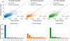 |
Fig. 15. Richness-independent feature set results at selected τ values (Section 4.3): τ = 2.0 Gyr for the past- and future-merger scores and τ = 1.0 Gyr for the full-merger score. Top: Predicted versus true merger scores for past-mergers (left), future-mergers (middle), and full-merger samples (right); the red dashed line indicates perfect prediction. Bottom: Permutation feature importances for the corresponding models; bars show the mean importance, and error bars show the standard deviation over 10 permutations. The red dashed line marks the 0.01 threshold used for feature selection. Features are labeled F1–F11, ranked by importance within each model. Their definitions are as follows: F1: Δv, F2: σr, 1, F3: σr, 2, F4: σv, 1, F5: σv, 2, F6: Δbic, F7: λ2/λ1, F8: z, F9: fm, F10: σr, F11: σv. |
4.4. Case study: Estimation of blue galaxy fraction
We matched our LoVoCCS cluster catalog (with cluster information obtained from the NASA/IPAC Extragalactic Database) to the eROSITA X-ray survey (Bulbul et al. 2024), and obtained the morphological disturbance score Dcomb from its associated morphology catalog (Sanders et al. 2025). Using a redshift-matching criterion of Δz < 0.01 and a maximum angular separation of 20 arcsec, we identified six matched clusters for this case study: Abell 4010, Abell 1651, Abell 1644, Abell 3558, Abell 3921, and RXCJ1539.5-8335. The matched sample is small, so we do not claim any statistically robust trend from this case study. We keep this section mainly as an example of how to apply our pipeline to observational datasets.
Due to the limited number of spectroscopic members, we relied on photometric redshifts for membership identification. We define members as galaxies within R500c, provided by Bulbul et al. 2024, and within a photometric redshift interval Δz = 0.05(1 + z). A magnitude cut at u, g < 23, 25 was applied. We excluded sources with photometric odds < 0.5, extendedness < 0.5, or maximum photometric magnitude error > 1.0, where the odds are defined as a measure of the width of the photo-z probability distribution (Benítez 2000), reflecting the confidence in photometric redshift estimation. Red-sequence galaxies were identified by fitting a linear relation in the (u − g) vs. g color-magnitude space. Galaxies that lie 0.2 magnitudes below this fitted red sequence are classified as blue.
In Fig. 16, we present the relation between the disturbance score and the blue galaxy fraction for the six matched clusters. The correlation appears weak, which is likely due to the use of photo-z estimates in place of spectroscopic redshifts. More robust results could be obtained with an expanded dataset, for example, through additional X-ray observations of LoVoCCS clusters in the future. We also note that leakage of field galaxies from our photometric redshift technique will lessen the correlation. Deeper and denser spectroscopic samples from the DESI (Dark Energy Spectroscopic Instrument) survey (DESI Collaboration 2024) and the upcoming Subaru Prime Focus Spectrograph (PFS) (Takada et al. 2014) would improve the observational limits here.
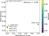 |
Fig. 16. Correlation between the morphological disturbance score (Dcomb) and the fraction of blue galaxies in six LoVoCCS clusters. Each point represents one cluster, colored by redshift. A weak negative correlation is observed (r = −0.08). Cluster names are annotated; the redshift is encoded by color. |
For comparison, we also evaluated the galaxy sample distribution obtained using only spectroscopic members under the same selection criteria, with Δz changed to Δz = 0.01(1 + z). We find that spectroscopic members tend to be systematically brighter and redder than the photometric sample, suggesting a potential selection bias when relying solely on spectroscopic redshifts that are currently available, as in Fig. 17.
 |
Fig. 17. Comparison of photometric and spectroscopic galaxy member samples across the six LoVoCCS clusters used in our case study. Left: g-band magnitude distribution. Middle: u-band magnitude distribution. Right: (u − g) color distribution. The histograms are normalized by sample size to show relative fractions. Galaxies with spectroscopic redshifts (orange) tend to be brighter and redder than the full photometric sample (blue), suggesting that spectroscopic samples preferentially include red sequence galaxies. |
To summarize, our method can, in principle, be applied to observational data, but several practical limitations need to be kept in mind. First, building an observational baseline requires a set of well-characterized ‘standard’ clusters with overlapping observational data (e.g., X-ray morphology measurements and sufficiently deep multiband photometry), and such samples can be rare. Second, observational magnitude limits and incomplete membership identification mean that we do not recover all member galaxies, which can bias any member-based summary statistics, thus affecting GMM fits and the resulting BIC-derived features. Finally, using spectroscopic redshifts for membership selection can introduce selection bias, while using photometric redshifts is more complete but comes with larger uncertainties; both effects can dilute correlations and reduce model performance.
4.5. Mass ratio estimator performance with future surveys
Upcoming weak-lensing surveys such as Rubin/LSST (Guy et al. 2025) and Roman/HLWAS (Akeson et al. 2019) are expected to achieve higher signal-to-noise ratios in aperture mass maps. This improvement will enhance the ability to identify multiple peaks, particularly in systems with lower merger mass ratios.
To assess the performance of our mass ratio estimator under such idealized conditions, we followed the procedure outlined in Section 3.4, but generated mock aperture mass maps without shape noise (i.e., background galaxies are assumed to have no intrinsic ellipticity).
We included all halos with M200c > 5 × 10¹³ M⊙, as well as halos with 1 × 10¹³ < M200c < 5 × 10¹³ M⊙ if their mass ratio exceeds 0.1. We then examined the correlation between our derived proxy quantity (see Eq. (13)) and the true merger mass ratio in this noise-free scenario, as illustrated in Fig. 18.
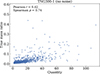 |
Fig. 18. Correlation between the proxy quantity and the true mass ratio in the TNG300-1 simulation, under noise-free conditions. Each point corresponds to an FOF halo. The Pearson correlation coefficient is r = 0.62 and the Spearman rank correlation is ρ = 0.74, indicating a strong monotonic relationship. |
Future observational advances should improve the reliability of merger identification. Upcoming redshift surveys and deeper/wider X-ray surveys will improve the detection of substructure and morphological asymmetries associated with mergers. Additionally, radio observations from MeerKAT (Jonas & MeerKAT Team 2016) and the upcoming SKA (Dewdney et al. 2009), as well as mock radio maps from simulations, may help distinguish between past and future mergers. For instance, symmetric radio relics may emerge after the first pericenter passage and thus serve as potential indicators of post-merger systems.
5. Conclusion
We present a phase-space machine learning method for identifying major mergers in galaxy clusters, using features derived from the projected radius–velocity distribution of member galaxies in the TNG-Cluster simulation. Trained on a disturbance score built from merger history, the model effectively captures structural disturbances but lacks sensitivity to merger timing, failing to distinguish between past and future events.
To address this, we explored time-sensitive observables, such as the curvature of the star formation rate (SFR) and the blue galaxy fraction. We find that the blue galaxy fraction decreases with increasing past-merger score, but shows no clear trend with future-merger score, suggesting its sensitivity to merger stage.
As a cross-check, we generated mock Chandra X-ray images and measured the BCG offset, which correlates strongly with the past-merger score but not with the future-merger score, supporting both the physical robustness of our score and the effectiveness of BCG offset as an indicator of past mergers.
Our results demonstrate that it is possible to determine the merger status of galaxy clusters based on the phase-space features and blue galaxy fraction. As a practical matter, application of these methods will only improve as additional spectroscopic, X-ray, and weak lensing data becomes available in the next decade.
Acknowledgments
We thank the developers of the publicly available scientific software used in this work, including NumPy (Harris et al. 2020), Pandas (The pandas development Team 2025), SciPy (Virtanen et al. 2020), Astropy (Astropy Collaboration 2022), Matplotlib (Hunter 2007), scikit-learn (Pedregosa et al. 2011), scikit-image (van der Walt et al. 2014), pyXSIM (ZuHone & Hallman 2016), SOXS (ZuHone et al. 2023), and yt (Turk et al. 2011). We also acknowledge the IllustrisTNG project for providing the simulation data. The IllustrisTNG simulations were undertaken with compute time awarded by the Gauss Centre for Supercomputing (GCS) under GCS Large-Scale Projects GCS-ILLU and GCS-DWAR on the GCS share of the supercomputer Hazel Hen at the High Performance Computing Center Stuttgart (HLRS), as well as on the machines of the Max Planck Computing and Data Facility (MPCDF) in Garching, Germany. This project used data obtained with the Dark Energy Camera (DECam), which was constructed by the Dark Energy Survey (DES) collaboration. This work is based on observations at Cerro Tololo Inter-American Observatory, NSF’s NOIRLab (NOIRLab Prop. ID 2019A-0308; PI: I. Dell’Antonio). This research is based on data obtained from the Astro Data Archive at NSF’s NOIRLab. This research has made use of the NASA/IPAC Extragalactic Database (NED), which is operated by the Jet Propulsion Laboratory, California Institute of Technology, under contract with the National Aeronautics and Space Administration. This work is based on data from eROSITA, the soft X-ray instrument aboard SRG, a joint Russian-German science mission supported by the Russian Space Agency (Roskosmos), in the interests of the Russian Academy of Sciences represented by its Space Research Institute (IKI), and the Deutsches Zentrum für Luft- und Raumfahrt (DLR). The SRG spacecraft was built by Lavochkin Association (NPOL) and its subcontractors, and is operated by NPOL with support from the Max Planck Institute for Extraterrestrial Physics (MPE). The development and construction of the eROSITA X-ray instrument was led by MPE, with contributions from the Dr. Karl Remeis Observatory Bamberg & ECAP (FAU Erlangen-Nuernberg), the University of Hamburg Observatory, the Leibniz Institute for Astrophysics Potsdam (AIP), and the Institute for Astronomy and Astrophysics of the University of Tübingen, with the support of DLR and the Max Planck Society. The Argelander Institute for Astronomy of the University of Bonn and the Ludwig Maximilians Universität Munich also participated in the science preparation for eROSITA. This research was conducted using computational resources and services at the Center for Computation and Visualization, Brown University. The analysis code used in this work is publicly available at https://github.com/KK-cloudhub/merger_trace.
References
- Akeson, R., Armus, L., Bachelet, E., et al. 2019, arXiv e-prints [arXiv:1902.05569] [Google Scholar]
- Aldás, F., Zenteno, A., Gómez, F. A., et al. 2023, MNRAS, 525, 1769 [CrossRef] [Google Scholar]
- Arendt, A. R., Perrott, Y. C., Contreras-Santos, A., et al. 2024, MNRAS, 530, 20 [Google Scholar]
- Astropy Collaboration (Price-Whelan, A. M., et al.) 2022, ApJ, 935, 167 [NASA ADS] [CrossRef] [Google Scholar]
- Bartalucci, I., Rossetti, M., Boschin, W., et al. 2024, A&A, 689, A324 [NASA ADS] [CrossRef] [EDP Sciences] [Google Scholar]
- Bartelmann, M., & Schneider, P. 2001, Phys. Rep., 340, 291 [Google Scholar]
- Benítez, N. 2000, ApJ, 536, 571 [Google Scholar]
- Botteon, A., Gastaldello, F., & Brunetti, G. 2018, MNRAS, 476, 5591 [Google Scholar]
- Bradač, M., Allen, S. W., Treu, T., et al. 2008, ApJ, 687, 959 [CrossRef] [Google Scholar]
- Bulbul, E., Liu, A., Kluge, M., et al. 2024, A&A, 685, A106 [NASA ADS] [CrossRef] [EDP Sciences] [Google Scholar]
- Chen, T., & Guestrin, C. 2016, arXiv e-prints [arXiv:1603.02754] [Google Scholar]
- Clowe, D., Bradač, M., Gonzalez, A. H., et al. 2006, ApJ, 648, L109 [NASA ADS] [CrossRef] [Google Scholar]
- Contreras-Santos, A., Knebe, A., Pearce, F., et al. 2022, MNRAS, 511, 2897 [NASA ADS] [CrossRef] [Google Scholar]
- Deshev, B., Finoguenov, A., Verdugo, M., et al. 2017, A&A, 607, A131 [NASA ADS] [CrossRef] [EDP Sciences] [Google Scholar]
- DESI Collaboration (Adame, A. G., et al.) 2024, AJ, 168, 58 [NASA ADS] [CrossRef] [Google Scholar]
- Dewdney, P. E., Hall, P. J., Schilizzi, R. T., & Lazio, T. J. L. W. 2009, IEEE Proc., 97, 1482 [Google Scholar]
- Englert, A., Dell’Antonio, I., Fu, S., et al. 2025a, Am. Astron. Soc. Meeting Abstr., 245, 412.07 [Google Scholar]
- Englert, A. M., Dell’Antonio, I., & Montes, M. 2025b, ApJ, 989, L2 [Google Scholar]
- Fu, S., Dell’Antonio, I., Chary, R.-R., et al. 2022, ApJ, 933, 84 [Google Scholar]
- Fu, S., Dell’Antonio, I., Escalante, Z., et al. 2024, ApJ, 974, 69 [Google Scholar]
- Fu, S., Dell’Antonio, I., Englert, A., et al. 2025, Am. Astron. Soc. Meeting Abstr., 246, 328.07 [Google Scholar]
- Ghizzardi, S., Rossetti, M., & Molendi, S. 2010, A&A, 516, A32 [NASA ADS] [CrossRef] [EDP Sciences] [Google Scholar]
- Golovich, N., Dawson, W. A., Wittman, D. M., et al. 2019, ApJ, 882, 69 [NASA ADS] [CrossRef] [Google Scholar]
- Guy, L. P., Bechtol, K., Bellm, E. C., et al. 2025, RTN-011: Rubin Observatory Plans for an Early Science Program, NSF-DOE Vera C. Rubin Observatory Technical Report [Google Scholar]
- Harris, C. R., Millman, K. J., van der Walt, S. J., et al. 2020, Nature, 585, 357 [NASA ADS] [CrossRef] [Google Scholar]
- Hetterscheidt, M., Erben, T., Schneider, P., et al. 2005, A&A, 442, 43 [NASA ADS] [CrossRef] [EDP Sciences] [Google Scholar]
- Hlavacek-Larrondo, J., Gendron-Marsolais, M. L., Fecteau-Beaucage, D., et al. 2018, MNRAS, 475, 2743 [NASA ADS] [CrossRef] [Google Scholar]
- Hunter, J. D. 2007, Comput. Sci. Eng., 9, 90 [NASA ADS] [CrossRef] [Google Scholar]
- Jones, C., & Forman, W. 1984, ApJ, 276, 38 [NASA ADS] [CrossRef] [Google Scholar]
- Katayama, H., Hayashida, K., Takahara, F., & Fujita, Y. 2003, ApJ, 585, 687 [Google Scholar]
- Lee, W., Pillepich, A., ZuHone, J., et al. 2024, A&A, 686, A55 [NASA ADS] [CrossRef] [EDP Sciences] [Google Scholar]
- Mantz, A. B., Allen, S. W., Morris, R. G., et al. 2014, MNRAS, 440, 2077 [NASA ADS] [CrossRef] [Google Scholar]
- Marinacci, F., Vogelsberger, M., Pakmor, R., et al. 2018, MNRAS, 480, 5113 [NASA ADS] [Google Scholar]
- McCleary, J., dell’Antonio, I., & Huwe, P. 2015, ApJ, 805, 40 [Google Scholar]
- Jonas, J., & MeerKAT Team 2016, MeerKAT Science: On the Pathway to the SKA, 1 [Google Scholar]
- Naiman, J. P., Pillepich, A., Springel, V., et al. 2018, MNRAS, 477, 1206 [Google Scholar]
- Nelson, D., Pillepich, A., Springel, V., et al. 2018, MNRAS, 475, 624 [Google Scholar]
- Nelson, D., Springel, V., Pillepich, A., et al. 2019, Comput. Astrophys. Cosmol., 6, 2 [Google Scholar]
- Nelson, D., Pillepich, A., Ayromlou, M., et al. 2024, A&A, 686, A157 [NASA ADS] [CrossRef] [EDP Sciences] [Google Scholar]
- Pedregosa, F., Varoquaux, G., Gramfort, A., et al. 2011, J. Mach. Learn. Res., 12, 2825 [Google Scholar]
- Pillepich, A., Nelson, D., Hernquist, L., et al. 2018, MNRAS, 475, 648 [Google Scholar]
- Planck Collaboration XIII. 2016, A&A, 594, A13 [NASA ADS] [CrossRef] [EDP Sciences] [Google Scholar]
- Poole, G. B., Fardal, M. A., Babul, A., et al. 2006, MNRAS, 373, 881 [Google Scholar]
- Prunier, M., Hlavacek-Larrondo, J., Pillepich, A., Lehle, K., & Nelson, D. 2024, MNRAS, 536, 3200 [Google Scholar]
- Rawle, T. D., Altieri, B., Egami, E., et al. 2014, MNRAS, 442, 196 [Google Scholar]
- Roberts, I. D. 2024, ApJ, 971, 182 [Google Scholar]
- Sanders, J. S., Bahar, Y. E., Bulbul, E., et al. 2025, A&A, 695, A160 [NASA ADS] [CrossRef] [EDP Sciences] [Google Scholar]
- Sanderson, A. J. R., Edge, A. C., & Smith, G. P. 2009, MNRAS, 398, 1698 [NASA ADS] [CrossRef] [Google Scholar]
- Sarazin, C. L. 2002, Astrophys. Space Sci. Libr., 272, 1 [Google Scholar]
- Schirmer, M. 2004, Ph.D. Thesis, Rheinische Friedrich-Wilhelms-Universität Bonn [Google Scholar]
- Schirmer, M., Erben, T., Schneider, P., Wolf, C., & Meisenheimer, K. 2004, A&A, 420, 75 [NASA ADS] [CrossRef] [EDP Sciences] [Google Scholar]
- Schwarz, G. 1978, Ann. Stat., 6, 461 [Google Scholar]
- Sobral, D., Stroe, A., Dawson, W. A., et al. 2015, MNRAS, 450, 630 [NASA ADS] [CrossRef] [Google Scholar]
- Stroe, A., Sobral, D., Dawson, W., et al. 2015, MNRAS, 450, 646 [NASA ADS] [CrossRef] [Google Scholar]
- Takada, M., Ellis, R. S., Chiba, M., et al. 2014, PASJ, 66, R1 [Google Scholar]
- The LSST Dark Energy Science Collaboration (Mandelbaum, R., et al.) 2018, arXiv e-prints [arXiv:1809.01669] [Google Scholar]
- The pandas development Team 2025, https://doi.org/10.5281/zenodo.3509134 [Google Scholar]
- Turk, M. J., Smith, B. D., Oishi, J. S., et al. 2011, ApJS, 192, 9 [NASA ADS] [CrossRef] [Google Scholar]
- van der Jagt, S., Osinga, E., van Weeren, R. J., et al. 2025, A&A, 699, A66 [NASA ADS] [CrossRef] [EDP Sciences] [Google Scholar]
- van der Walt, S., Schönberger, J. L., Nunez-Iglesias, J., et al. 2014, PeerJ, 2 [Google Scholar]
- van Weeren, R. J., de Gasperin, F., Akamatsu, H., et al. 2019, Space Sci. Rev., 215, 16 [Google Scholar]
- Virtanen, P., Gommers, R., Oliphant, T. E., et al. 2020, Nat. Methods, 17, 261 [Google Scholar]
- Wen, Z. L., Han, J. L., & Yuan, Z. S. 2024, MNRAS, 532, 1849 [Google Scholar]
- Wilber, A., Brüggen, M., Bonafede, A., et al. 2019, A&A, 622, A25 [NASA ADS] [CrossRef] [EDP Sciences] [Google Scholar]
- ZuHone, J. A., & Hallman, E. J. 2016, Astrophysics Source Code Library [record ascl:1608.002] [Google Scholar]
- ZuHone, J. A., Kowalik, K., Öhman, E., Lau, E., & Nagai, D. 2018, ApJS, 234, 4 [NASA ADS] [CrossRef] [Google Scholar]
- ZuHone, J. A., Vikhlinin, A., Tremblay, G. R., et al. 2023, Astrophysics Source Code Library [record ascl: 2301.024] [Google Scholar]
All Figures
|
Fig. 1. Mock X-ray images of FOF halo 0 from three projections (X, Y, and Z), centered on the group position and smoothed to a ∼10 kpc resolution. Black dots mark the centers used for cropping. A 1000 kpc scale bar is shown in each panel. The color indicates the photon counts, normalized using logarithmic scaling. |
| In the text | |
|
Fig. 2. Example mock observation from the TNG300-1 simulation. A 500 kpc scale bar is shown in each panel. Left: Simulated aperture mass map (S/N) of FOF halo 142, with R200c ∼ 750kpc, incorporating shape noise consistent with observational weak lensing data. For visualization, the maps are Gaussian-smoothed with a kernel scale of ∼60 kpc; this smoothing is applied for display purposes only. Right: Surface mass density map (dark matter + gas) in units of log M⊙/pixel. The positions of the central and the most massive satellite subhalos are marked for reference. |
| In the text | |
|
Fig. 3. Model performance as a function of τ, evaluated using three target score definitions: past-merger (left), future-merger (middle), and full-merger (right) scores. Orange lines show the R2 on the training set, and blue lines show the R2 on the test set. All results are based on the rotated projection configuration described in Section 3.1.1. |
| In the text | |
|
Fig. 4. Test R2 as a function of the time window length for the past-, future-, and full-merger scores. The right panel summarizes the phase-space input features used in the model. |
| In the text | |
|
Fig. 5. Comparison of permutation feature importance rankings for models using the three merger score definitions: past-merger (left), future-merger (middle), and full-merger (right) scores. Bars indicate the mean importance of each feature, with error bars representing the standard deviation over 10 independent permutations. The red dashed line marks the 0.01 threshold used for feature selection. Features are labeled F1–F17, ranked by importance within each model. Their definitions are as follows: F1: ΔR, F2: v1, F3: v2, F4: Δv, F5: σr, 1, F6: σr, 2, F7: σv, 1, F8: σv, 2, F9: fn, F10: bic1, F11: bic2, F12: Δbic, F13: λ2/λ1, F14: z, F15: fm, F16: σr, F17: σv. |
| In the text | |
|
Fig. 6. Predicted merger scores versus true scores for three test sets: on past-merger (left), future-merger (middle), and full-merger (right) scores. The red dashed line indicates the ideal case of perfect prediction. Each panel also displays the R2 score for the corresponding test. Points are slightly transparent to indicate density. The model shows consistent predictive performance across different temporal subsets. High true scores tend to be underpredicted. This is mainly because the strongly skewed true-score distribution (Fig. 7): most halos have low scores, which dominate the training and bias the predictions toward low values. |
| In the text | |
|
Fig. 7. Distribution of true merger scores for the full sample (filled bars) and the test sample (outlined bars), shown for the past-merger, future-merger, and full-merger datasets. |
| In the text | |
|
Fig. 8. Curvature of the normalized SFR as a function of merger score. The left and right panels show results for the past- and future-merger scores, respectively. In each case, the score distribution is divided into five quantile bins. A total of 9812 samples are used in the past-merger analysis and 5609 in the future-merger case. Error bars indicate the standard error of the mean curvature within each bin. |
| In the text | |
|
Fig. 9. Fraction of blue galaxies as a function of merger score, shown separately for past-merger scores (left) and future-merger scores (right). Each curve corresponds to a redshift bin defined as [zlow, zhigh), i.e., including the lower bound but excluding the upper bound. Within each redshift bin, the score distribution is divided into five quantile bins. Error bars indicate the standard error of the mean blue fraction within each merger score bin. Several redshift bins are absent in the future-merger panel due to the exclusion of low-redshift samples (z < 0.15). |
| In the text | |
|
Fig. 10. Mean BCG offset as a function of merger score under three definitions: past-merger (left), future-merger (middle), and full-merger (right) scores. Each point represents the average offset within a merger score bin, with vertical bars indicating the standard error of the mean. The total sample size is 325 clusters. To ensure roughly equal sample counts in each bin, we apply quantile-based binning: full- and past-merger scores are divided at [0.0, 0.2, 0.4, 0.6, 0.8, 1.0]; future-merger scores are divided at [0.0, 0.3, 0.48, 0.66, 0.84, 1.0] due to the heavy concentration near zero. A clear positive trend is visible in the first panel, suggesting that BCG displacement increases with merger activity based on past events. |
| In the text | |
|
Fig. 11. Correlation between the quantity, i.e., q in Equation 13, and the true merger mass ratio. Left: Results from TNG300-1 halos. Right: LoVoCCS observed clusters. Each point represents a galaxy cluster; the x-axis shows the quantity estimator defined in Eq. (13), and the y-axis shows the true mass ratio. We report both Pearson r and Spearman ρ correlation coefficients to characterize the relationship. |
| In the text | |
|
Fig. 12. Model performance as a function of τ, evaluated using three target score definitions: past-merger (left), future-merger (middle), and full-merger (right) scores. Orange and blue curves show the training and test R2, respectively, and gray histograms indicate the sample count. This test uses the leakage-minimized split (grouping by halo ID only, so that progenitors and descendants of training halos are excluded from the test set) together with the rotation-based filtering scheme for sample selection. |
| In the text | |
|
Fig. 13. Model performance as a function of τ, evaluated using three target-score definitions: past-merger (left), future-merger (middle), and full-merger (right) scores. Orange and blue curves show the training and test R2, respectively, and gray histograms indicate the sample count. These tests assess projection robustness. Top: Treating the three orthogonal projections of each halo as independent samples, using the leakage-minimized split (grouping by halo ID). Bottom: Following the setup in Section 3.1.1 (grouping by halo ID and snapshot number and using rotation-based filtering), the projection-rotation order is changed from [z, drop, x, drop, y, drop] to [x, drop, y, drop, z, drop]. The similar performance suggests that the model is not sensitive to the projection order, which is favorable for observational applications where only one projection is available. |
| In the text | |
|
Fig. 14. Model performance as a function of τ, evaluated using three target-score definitions: past-merger (left), future-merger (middle), and full-merger (right) scores. Orange and blue curves show the training and test R2, respectively, and gray histograms indicate the sample count. The train–test split and sample selection follow Section 3.1.1 (grouping by halo ID and snapshot number) with rotation-based filtering. |
| In the text | |
|
Fig. 15. Richness-independent feature set results at selected τ values (Section 4.3): τ = 2.0 Gyr for the past- and future-merger scores and τ = 1.0 Gyr for the full-merger score. Top: Predicted versus true merger scores for past-mergers (left), future-mergers (middle), and full-merger samples (right); the red dashed line indicates perfect prediction. Bottom: Permutation feature importances for the corresponding models; bars show the mean importance, and error bars show the standard deviation over 10 permutations. The red dashed line marks the 0.01 threshold used for feature selection. Features are labeled F1–F11, ranked by importance within each model. Their definitions are as follows: F1: Δv, F2: σr, 1, F3: σr, 2, F4: σv, 1, F5: σv, 2, F6: Δbic, F7: λ2/λ1, F8: z, F9: fm, F10: σr, F11: σv. |
| In the text | |
|
Fig. 16. Correlation between the morphological disturbance score (Dcomb) and the fraction of blue galaxies in six LoVoCCS clusters. Each point represents one cluster, colored by redshift. A weak negative correlation is observed (r = −0.08). Cluster names are annotated; the redshift is encoded by color. |
| In the text | |
|
Fig. 17. Comparison of photometric and spectroscopic galaxy member samples across the six LoVoCCS clusters used in our case study. Left: g-band magnitude distribution. Middle: u-band magnitude distribution. Right: (u − g) color distribution. The histograms are normalized by sample size to show relative fractions. Galaxies with spectroscopic redshifts (orange) tend to be brighter and redder than the full photometric sample (blue), suggesting that spectroscopic samples preferentially include red sequence galaxies. |
| In the text | |
|
Fig. 18. Correlation between the proxy quantity and the true mass ratio in the TNG300-1 simulation, under noise-free conditions. Each point corresponds to an FOF halo. The Pearson correlation coefficient is r = 0.62 and the Spearman rank correlation is ρ = 0.74, indicating a strong monotonic relationship. |
| In the text | |
Current usage metrics show cumulative count of Article Views (full-text article views including HTML views, PDF and ePub downloads, according to the available data) and Abstracts Views on Vision4Press platform.
Data correspond to usage on the plateform after 2015. The current usage metrics is available 48-96 hours after online publication and is updated daily on week days.
Initial download of the metrics may take a while.