| Issue |
A&A
Volume 707, March 2026
|
|
|---|---|---|
| Article Number | A341 | |
| Number of page(s) | 14 | |
| Section | Extragalactic astronomy | |
| DOI | https://doi.org/10.1051/0004-6361/202555934 | |
| Published online | 18 March 2026 | |
Chemodynamical properties of gas-rich galaxies: A comparison of observations and simulations
1
Institute of Astronomy, Kharkiv National University, Svobody Sq. 4, Kharkiv 61022, Ukraine
2
Department of Astronomy, University of Geneva, Chemin Pegasi 51, 1290 Versoix, Switzerland
3
Institute of Physics, Laboratory of Astrophysics, École Polytechnique Fédérale de Lausanne (EPFL), 1290 Sauverny, Switzerland
4
European Southern Observatory, Karl-Schwarzschild Str. 2, 85748 Garching bei München, Germany
5
European Southern Observatory, Alonso de Córdova 3107, Casilla, 19001 Vitacura, Santiago, Chile
6
French-Chilean Laboratory for Astronomy, IRL 3386, CNRS and U. de Chile, Casilla 36-D, Santiago, Chile
7
Centre de Recherche Astrophysique de Lyon, Univ. Claude Bernard Lyon 1, 9 Av. Charles André, 69230 Saint-Genis-Laval, France
8
Max-Planck-Institut für Astrophysik, Karl-Schwarzschild-Str. 1, 85748 Garching b. München, Germany
★ Corresponding author: This email address is being protected from spambots. You need JavaScript enabled to view it.
Received:
13
June
2025
Accepted:
3
February
2026
Abstract
We performed a comprehensive analysis of the chemical and dynamical properties of quasar-damped Lyman-α (DLA) galaxies and compare these to the GEAR chemodynamical simulations. Specifically, we aim to constrain the behavior of α-element enhancements with metallicity, the dependence of [α/Fe] on the specific star formation rate (sSFR), and the absorption-line velocity widths (Δv90) versus stellar mass, Δv90 versus metallicity, and mass–metallicity relations. For the comparison, we selected five galaxies simulated with the chemodynamical Tree-SPH code GEAR with stellar masses in the range of 6.1 ≤ log M★/M⊙ ≤ 10.8 and at six different redshifts between 0.33 and 4.12. We find that the abundance ratios [α/Fe] and [M/H] observed in the interstellar medium (ISM) of DLA galaxies overlap with the abundance trends in gas of the simulated galaxies. Our findings corroborate a picture in which DLAs with Δv90 below and above 100 km s−1 trace galaxies with masses in the ranges of 6 < log M★ < 8 and 8 < log M★ < 11, respectively. We suggest that observations should be used with caution when constraining the theoretical [α/Fe] versus sSFR relations because of systematics (if abundances are obtained from emission lines) or differences in the gas properties as probed by a DLA and its counterpart. So far, only the observations in absorption of inner gas of the LMC and SMC are in agreement with the simulated data. We confirm that DLAs detected at large impact parameters most likely probe the gas of satellite or other halo galaxies which are adjacent to the central galaxy. We further find that the velocity widths versus stellar masses and mass–metallicity relations agree well with observations, while GEAR should be calibrated more carefully to reproduce the Δv90 versus metallicity relation. To place our results in context, we additionally incorporated chemodynamical properties of a few selected model galaxies obtained from other simulations.
Key words: ISM: abundances / dust, extinction / galaxies: abundances / galaxies: evolution
© The Authors 2026
 Open Access article, published by EDP Sciences, under the terms of the Creative Commons Attribution License (https://creativecommons.org/licenses/by/4.0), which permits unrestricted use, distribution, and reproduction in any medium, provided the original work is properly cited.
This article is published in open access under the Subscribe to Open model. This email address is being protected from spambots. You need JavaScript enabled to view it. to support open access publication.
1. Introduction
The chemical evolution of galaxies is a complex problem that involves many astrophysical aspects such as metal abundances in stars and gas, gas content and flows, dust quantity, stellar masses, star formation rate (SFR), stellar feedback, interaction with other galaxies, and so on (Tinsley 1980; Matteucci 2012). The study of metal enrichment of gas and stars in galaxies, together with information about their stellar masses and SFRs, provides clues to the internal processes that govern the chemical evolution of the galaxies. Indeed, [α/Fe] versus [M/H] are important diagnostics for the chemical evolution of galaxies (Kobayashi et al. 2020). Iron and α elements are formed via different channels with different timescales. Core-collapse supernovae (CCSNe) are the main source producing α elements at an early stage of galaxy evolution, which results in enhanced [α/Fe]. Type Ia supernovae (SNe Ia), dominating the iron enrichment, begin to contribute with a time delay of ∼1 Gyr, and the [α/Fe] ratio begins to decrease (e.g., Worthey et al. 1992; McWilliam 1997; Matteucci 2012). The turning point in the [α/Fe] versus [M/H] plot that separates these two regimes is called the “high-α knee”. Theoretically, the position of the knee is sensitive to the early star formation history (SFH), and it should move toward higher metallicity with increasing SFR (Tinsley 1979; McWilliam 1997).
The processes taking place in the Milky Way (MW) and nearby galaxies have been studied in detail from spectroscopic observations of individual stars (e.g., McWilliam 1997; Tolstoy et al. 2009; de Boer et al. 2014; Hasselquist et al. 2021). It has been shown that nearby dwarf galaxies have high-α knees at different metallicities, and this depends not only on the mass of the galaxies, but also on SNe feedback, galactic winds, and interaction with other galaxies, which ultimately influences the SFH (Tolstoy et al. 2009).
Unfortunately, in distant galaxies it is normally not possible to obtain information about individual stars1. Revealing the chemical properties of distant galaxies can be done from studies of the integrated stellar population or the interstellar medium (ISM).
A unique way to study the chemical properties of the ISM in distant galaxies is from observations of damped Lyman-α (DLA; Wolfe et al. 2005) absorbers defined as systems with high column densities of neutral hydrogen (N(HI) ≥ 2 × 1020 cm−2) that appear in absorption of quasi-stellar objects (QSOs) spectra. DLAs are fundamental for the study of galaxies, because they bear the bulk of neutral hydrogen in the Universe (e.g., Wolfe et al. 1995) and metals at high redshifts (Péroux et al. 2020). DLAs are associated with galaxies with a wide mass range, including low-mass galaxies (with stellar masses likely down to 106 M⊙ Christensen et al. 2014; Krogager et al. 2017; Møller & Christensen 2020), which in number are the majority (Fontana et al. 2006). Recently, we used gas observed in absorption in QSO-DLA sources to study the chemical evolution of distant galaxies (Velichko et al. 2024). We analyzed [α/Fe] and [M/H] in the neutral ISM (CGM) of 24 QSO-DLAs at redshifts in the 1.6 < z < 3.4 range.
The weak spot in the study of DLAs is the difficulty in measuring parameters such as luminosity, stellar mass, and SFR of the corresponding galaxies. It is becoming more evident that correlations between these fundamental parameters and metallicity are crucial to understanding the nature of galaxies at different redshifts (e.g., Tremonti et al. 2004; Savaglio et al. 2005; Calura et al. 2009; Henry et al. 2021; Kashino et al. 2022; Scholte et al. 2024; Chemerynska et al. 2024; Curti et al. 2024). To measure them, observations in emission of the DLA counterparts are needed (Fynbo et al. 2008). Many attempts have been made to identify the galaxies responsible for the DLA absorption lines (Djorgovski et al. 1996; Møller et al. 2002; Ma et al. 2015; Kulkarni et al. 2022), but only very few have been detected in emission (Krogager et al. 2017).
Alternatively, the properties of DLAs can be constrained by comparing their measured characteristics with those obtained from modeling. Analytical models are used to test the origin of DLAs (Prochaska & Wolfe 1997; Jedamzik & Prochaska 1998; Maller et al. 2001); they are successful in reproducing general observed characteristics of DLAs such as observed metallicity distributions (Fynbo et al. 2008; Krogager & Noterdaeme 2020) and distributions of cold and warm neutral gas (Krogager & Noterdaeme 2020). A limitation is that these models depend on the average scaling ratios of galaxies and cannot capture processes related to galactic substructure or gas structures in the intergalactic medium (Rhodin et al. 2019).
Cosmological hydrodynamical simulations seem to be more capacious and efficient in constraining galaxy properties and relations obtained from observations (e.g., Nagamine et al. 2007; Pontzen et al. 2008; Fumagalli et al. 2011; Cen 2012; Rahmati et al. 2013; Hummels et al. 2013; Faucher-Giguère et al. 2015; Liang et al. 2016; Revaz & Jablonka 2018; Roca-Fàbrega et al. 2021). Modern cosmological hydrodynamical simulations have been successfully used to study properties of the ISM (e.g., Altay et al. 2013; Rhodin et al. 2019; Hassan et al. 2020; Garratt-Smithson et al. 2021; Klimenko et al. 2023) and CGM (Oppenheimer et al. 2012; Stinson et al. 2012; Shen et al. 2012, 2013; Oppenheimer et al. 2016) in distant galaxies. It is challenging to reproduce all the diversity of observed galaxy properties and their evolution with redshift because of the complexity of mechanisms governing the formation and evolution of galaxies. Hydrodynamical models must govern interactions between multiple constituents such as gas inflow, gas cooling, UV-background heating, hydrogen self-shielding, star formation, and associated feedback, which creates gas outflows.
In this work, we performed a comprehensive analysis of the chemical and dynamical properties of DLA galaxies studied in our previous work (Velichko et al. 2024), as well as those found in the literature (Weng et al. 2023; Berg et al. 2023; Kulkarni et al. 2022; Møller & Christensen 2020; Christensen et al. 2014; Rahmati & Schaye 2014; Krogager et al. 2013; Fynbo et al. 2013, 2011), by comparing them with simulations developed by Revaz & Jablonka (2012), Revaz et al. (2016), and Revaz & Jablonka (2018) using the chemodynamical Tree-SPH code GEAR. We constrained the observed galaxy properties within the stellar mass range of 6.1 ≤ log(M★/M⊙)≤10.8 and at redshifts of 0.33 ≤ z ≤ 4.12.
The paper is organized as follows. In Sect. 2, we describe the observed and simulated data that we compared. The methods we applied to extract physical properties and make mock observations from the simulations are described in Sect. 3. In Sect. 4, we compare observations and simulations of some scaling relations that are relevant for the study of galaxy evolution. The mass estimations of the 24 DLAs analyzed in our previous study are given in Sect. 4.1.1; we compared their observed [α/Fe]–metallicity distribution with the corresponding trends predicted by the GEAR simulations. Finally, the main conclusions are reported in Sect. 5.
2. Data
2.1. Observed [α/Fe] versus [M/H] in the ISM of DLAs
In our previous work (Velichko et al. 2024), we analyzed abundance patterns of the neutral ISM in a sample of 110 QSO-DLA sources. From there, we selected 24 objects to be part of what we call the “golden” sample, for which column densities of Ti and at least one more α element were measured. This requirement was needed in order to apply the method developed by De Cia et al. (2024) to reliably calculate the total (gas + dust) metallicity [M/H]tot as well as relative abundances of chemical elements (O, Mg, Si, S, Ti, Cr, Fe, Ni, Zn, P, and Mn) with respect to iron corrected for the depletion by dust, [X/Fe]nucl. In particular, the measurement of Ti specifically allows the characterization of the dust-corrected α-element abundances, and thus the derivation of [α/Fe]nucl. In Sect. 4.1.1, we compare the observed values of [α/Fe]nucl versus [M/H]tot with those obtained from the GEAR simulations.
2.2. Kinematics as a proxy for the dynamical mass
The masses of the DLA galaxies we studied in our previous work (Velichko et al. 2024) are mostly unknown, with two exceptions (Q2243−605 and Q2206−1985, which are the most metal-rich and probably most massive galaxies measured by Møller & Christensen 2020), because it is very difficult to detect their counterparts in emission. Instead, as a mass indicator, we used velocity widths of Δv90 measured from low-ionization line profiles provided by Ledoux et al. (2006) (see Table 1 from Velichko et al. 2024). The argument for using Δv90 of DLAs as a proxy for the gravitational masses of their hosts is the existence of the velocity width–metallicity correlation obtained by Ledoux et al. (2006), which is the consequence of an underlying mass–metallicity correlation. This was validated by Christensen et al. (2014), which measured the masses of a dozen DLA counterparts. The combined mass–velocity width correlation was also confirmed by Haehnelt et al. (1998) from simulations. According to the virial theorem, line-of-sight galaxy velocities provide a measure of the depth of the potential well (e.g., Saro et al. 2013). All the correlations have a large scatter naturally caused by a variety of impact parameters, inclination angles, presence of infall (outflow) of gas, merging galaxy sub-clumps, dependence on redshift, and so on. probed by the observations. Considering all these factors, Δv90 is only a rough proxy of the galaxy mass.
2.3. Simulations
2.3.1. GEAR
To constrain the properties of the DLA galaxies studied in Velichko et al. (2024), we used model galaxies simulated with the chemodynamical Tree-SPH code GEAR developed by Revaz & Jablonka (2012) and Revaz et al. (2016), which takes into account the complex treatment of baryon physics. In a nutshell, the gas cooling is computed using the GRACKLE library (Smith et al. 2017) that contains primordial gas and metal-line cooling, as well as H2. UV-background radiation (Haardt & Madau 2012) and hydrogen self-shielding are both included. Star formation is modeled using a standard stochastic prescription (Katz 1992; Katz et al. 1996) that reproduces the Schmidt law. It is supplemented by a Jeans pressure floor adding a nonthermal term to the equation of state. The stellar feedback includes both Type Ia and II SNe with yields taken from Tsujimoto et al. (1995). Both Ia and II SNe explode as individual stars. For type II, the explosion time is precisely the end of the star’s lifetime. For SNIa, we used the rates from Kobayashi et al. (2000), where explosions started after 300 Myr at the earliest, following the star formation with the corresponding IMF. To prevent an instantaneous radiation of the injected energy, a delayed cooling method was used. It consists iof disabling gas cooling for a short period of time (Stinson et al. 2006), here taken as 5 Myr, after the explosion event.
The GEAR simulations have been tested in the works of Revaz & Jablonka (2018) and Roca-Fàbrega et al. (2021). By comparing with observations of the Local Group dwarf galaxies, Revaz & Jablonka (2018) showed that the scaling relations between integrated properties of the GEAR simulated galaxies, such as their total V-band luminosity, stellar line-of-sight velocity dispersion, stellar mean metallicity, gas-mass content, and half-light radius are well reproduced over several orders of magnitude. Moreover, a good match between six selected Local Group dwarf galaxies and the corresponding GEAR models in detailed stellar properties, such as [Mg/Fe] versus [Fe/H] (where Mg is used as a proxy of α-elements), radial distribution of the stellar line-of-sight velocity dispersion, and the stellar metallicity distribution proves the validity of the GEAR simulations, at least in the low-mass range of 106 − 109 M⊙ (Revaz & Jablonka 2018). The stellar [Mg/Fe] versus [Fe/H] relation traces the SFH in galaxies, and the fact that it is well reproduced for the real dwarf galaxies (see Fig. 10 in Revaz & Jablonka 2018) shows that the evolution of the stellar population and chemical enrichment implemented in GEAR match well with observations of dwarf galaxies. The MW-mass GEAR galaxy has also been analyzed and compared with other simulations within the Assembling Galaxies Of Resolved Anatomy (AGORA) project (Kim et al. 2016; Roca-Fàbrega et al. 2021), where its ability to simulate MW-like galaxies is demonstrated.
From the 27 dwarf galaxies from the zoom-in GEAR simulations presented in Revaz & Jablonka (2018), we selected four with stellar masses in the range of 6.1 ≤ log M★ ≤ 8.7 (at z = 0) – h074, h050, h076, and h026 (from least to most massive) – in such a way as to cover the low-mass end of the DLA sample described in Sect. 2.1. To expand the range under study toward higher masses, we selected a MW-like galaxy h000 of log M★ = 10.8 (at z = 0) from Roca-Fàbrega et al. (2021), also simulated with the GEAR code, but with a slightly stronger feedback than in the dwarf galaxies mentioned above. To trace the galaxy properties over their lifetimes, we analyzed six snapshots corresponding to z = 4.12, 3.49, 2.55, 2.01, 1.15, and 0.33. Each snapshot contains information on the physical, chemical, and kinematic properties of stellar and gas particles. In this work, we focused on the properties of the gas, which is modeled in the simulations as gas “particles” with initial masses of a few × 104 M⊙ (Revaz & Jablonka 2018; Roca-Fàbrega et al. 2021). The data also include information on abundances of some chemical elements contained in gas (Fe, Mg, O, S, Zn, Sr, Y, Ba, Eu) calculated with the use of theoretical yields from Tsujimoto et al. (1995) and Kobayashi et al. (2000). Further details on the numerical characteristics of the GEAR models can be found in Appendix A.
2.3.2. Other simulations
This paper focuses on the comparison of observed DLA properties with GEAR simulated galaxies. As every simulation, GEAR has its own assumptions and limitations. We included comparisons with other simulations to test other physical implementations. We found a few galaxy characteristics in the literature that are suitable for comparison, obtained by other authors from AURIGA (van de Voort et al. 2019), IllustrisTNG (Nelson et al. 2020; Torrey et al. 2019), performed using the AREPO code, and EAGLE (Matthee & Schaye 2018), which uses the modified GADGET-3 code. We also included the Overwhelmingly Large Simulations (OWLS, Schaye et al. 2010) in the comparison; these are based on the GADGET-3 code and were modified by Rahmati & Schaye (2014). All the models may not be representative of a full sample of simulated galaxies. With this comparison, we intend to explore alternatives for GEAR and trace how different prescriptions affect galaxy properties.
To help in the comparison of those different models, we briefly highlight the main properties and difference of their physical model. AURIGA and TNG50 use baryon particles with an initial mass of ∼4 ⋅ 104 M⊙ and ∼8 ⋅ 104 M⊙, respectively. Both models were built on the moving mesh AREPO code and share very similar physics. The ISM is described by the subgrid model (Springel & Hernquist 2003), in which star-forming gas is treated as a two-phase medium. They also both inject stellar feedback as energy-driven winds with, however, slightly different parameters. The EAGLE simulations are slightly less resolved (∼2 ⋅ 106 M⊙), as such, they marginally resolve the Jeans scales in the warm ISM. The stellar feedback is based on a stochastic thermal-feedback approach (Dalla Vecchia & Schaye 2012) that efficiently triggers outflows without the need to turn off radiative cooling temporarily.
With a stellar mass resolution of 103 M⊙, GEAR has the highest resolution. GEAR is also the only code that explicitly resolves the multiphase nature of cold gas with temperatures down to 10 K, including hydrogen self-shielding.
3. Methods
First, for each simulated galaxy, we determined a characteristic radius within which most of the gas belonging to a given galaxy is enclosed. From Fig. 1, showing the surface density of gas in the simulated galaxies, one can see that gas particles are mostly concentrated within ∼2 kpc of the center in dwarf galaxies and ∼5 − 10 kpc in the MW-like galaxy h000.
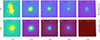 |
Fig. 1. The surface density of all gas for the five GEAR galaxies (Revaz & Jablonka 2018; Roca-Fàbrega et al. 2021) at redshifts 4.12 (upper panel) and 0.33 (lower panel). For h074, the lower rightmost panel is empty, as all the gas has been removed by photoevaporation. |
The galaxy h000 has an elongated shape at z = 4.12 (upper leftmost panel in Fig. 1), because at that moment it was made of two merging galaxies that doubled the volume occupied by the gas. The galaxies had merged completely by z = 4. For the least massive galaxy, h074 (lower rightmost panel in Fig. 1), due to the presence of the UV background, the ISM was gradually fully ionized and heated, reaching a point where its specific energy exceeded the gravitational binding energy of the dwarfs. Consequently, it gradually left the system (evaporated), and so the gas properties at z = 1.15 and 0.33 could not be studied.
3.1. Determining H I column densities
To obtain H I column densities in the simulated galaxies, we used TRIDENT, a parallel, Python-based open-source code for producing synthetic observations from astrophysical hydrodynamical simulation outputs (Hummels et al. 2017). By creating a ray of light along a chosen line of sight crossing a galaxy, TRIDENT generates an absorption spectrum arising from interaction with intervening material that makes up the ISM. An illustration of the method is given in Fig. B.1. To build statistics, we created light rays crossing each simulated galaxy at different galactocentric distances with a step of 0.1 kpc for dwarf galaxies or 0.2 kpc for the galaxy h000. We repeated this procedure for six different orientations spaced by 30° around the x, y, and z axes in such a way that it mimicked 18 viewing angles. Then, at each galactocentric distance, we calculated the H I column density averaged over the 18 lines of sight. Finally, we defined the DLA size of each model galaxy as the volume within which the H I column density was high enough to correspond to DLA (i.e., log N(H I) > 20.3).
3.2. Determining velocity widths
To determine velocity widths of the TRIDENT-generated absorption lines, Δv90, in the simulated galaxies, we applied the method described in Ledoux et al. (2006). Because the GEAR simulations do not provide the number densities for ionized species of the Fe II, S II, Si II, and O I ions (normally used to obtain Δv90 from DLA observations), we created them from the total metallicity using the TRIDENT function add_ion_fields, assuming collisional ionization equilibrium and photoionization in the optically thin limit from a redshift-dependent metagalactic UV background. To compute each ion fraction as a function of density, temperature, metallicity, and redshift, TRIDENT uses the CLOUDY software (see Hummels et al. 2017, for details).
Next, we created absorption spectra produced by transitions from the ground states of the ions Fe II, S II, Si II, and O I (according to the list in Table C.1) along each line of sight. Among the lines, we selected those that are neither strongly saturated nor too weak and transformed them into the velocity space. To make it more realistic and comparable to the observed data (Velichko et al. 2024), when creating the spectrum, we chose the resolution Δv to be 6 km s−1, which corresponds to R ≃ 50 000 and is comparable to UVES, and we added Gaussian random noise and fixed the signal-to-noise ratio (S/N) as equal to 30. Then we calculated the apparent optical depth and determined Δv90 as v(95%) − v(5%), as shown in Fig. C.1, where v(5%) and v(95%) are the relative velocities corresponding to the fifth and 95th percentiles of the cumulative apparent optical depth.
3.3. Determining [Fe/H] and [Mg/Fe]
To analyze chemical properties of gas in simulated galaxies, we used the parallelized Python package pNbody (Revaz 2013)2, a toolbox to manipulate and display very large N-body systems interactively. The GEAR output includes abundances of some chemical elements produced by stars and released into the ISM through Type Ia and II supernova explosions. To compare with the results obtained from observations by Velichko et al. (2024), we were mainly interested in analyzing Fe and α elements. To obtain the element abundances contained in gas in the simulated galaxies, we selected gas particles located inside the DLA volume defined from the distribution of H I column densities, as described in Sect. 3.1, and computed the mean and dispersion of the relative abundances [Fe/H] and [Mg/Fe] (where Mg is used as a proxy for α elements; Revaz & Jablonka 2018).
4. Results and discussion
4.1. Chemical properties
4.1.1. [α/Fe] versus [M/H]
In our previous work, Velichko et al. (2024), we analyzed abundance patterns in DLA galaxies and separated our golden sample (see the data description in Sect. 2.1) into two groups based on the absorption kinematics, one with the velocity widths Δv90 < 100 km s−1 (low Δv90) and the other with Δv90 > 100 km s−1 (high Δv90). We used Δv90 as a proxy for the galaxy mass due to a lack of measurements of the latter (see Sect. 2.2). To quantify the breakpoint in Δv90, Velichko et al. (2024) used the empirical relation obtained by Arabsalmani et al. (2016), according to which Δv90 of 100 km s−1 corresponds to the galactic stellar mass of 109 M⊙3. In Velichko et al. (2024), we found a quantitative difference in the distribution of [α/Fe]nucl versus [M/H]tot between low- and high-Δv90 subsamples, such that less massive galaxies show an α-element knee at lower metallicities than more massive galaxies.
Figure 2 shows the [α/Fe]nucl versus [M/H]tot relations of the GEAR simulated galaxies (as 1σ confidence intervals), together with the DLA values that we measured in Velichko et al. (2024). We used this comparison to constrain the masses of the DLA galaxies. The simulated data show a trend in metallicity with mass: as the galaxy mass increases, the area tends to shift toward higher metallicity because more massive galaxies enrich their surrounding gas with metals more rapidly, which is consistent with theoretical expectations and observations. Indeed, in Velichko et al. (2024), by dividing the QSO-DLA sample into low- and high-Δv90 subsamples, we found that more massive galaxies showed the high-α knee to be at higher metallicity compared to less massive galaxies. Overall, the observed abundance ratios almost completely overlapped with the output of the simulations, so we conclude that the α-element abundances observed in our sample of DLA galaxies are consistent with stellar masses in the ranges of 106 − 108 M⊙ (h074, h050, h076) and 108 − 1011 M⊙ (h076, h026, h000) for the low- and high-Δv90 subsamples, respectively.
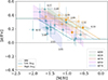 |
Fig. 2. [α/Fe] versus metallicity. Shaded area: [Mg/Fe] versus [Fe/H] in gas of five simulated galaxies h000, h026, h076, h050, and h074 at z from 4.12 to 0.33 (see the numbers). In the case of h074, there were no gas particles left at z < 2.01. Open orange diamonds and open blue triangles show the values [α/Fe]nucl obtained by Velichko et al. (2024) from the observations of the ISM in QSO-DLAs in the high- and low-Δv90 subsamples, respectively. Filled symbols mark DLAs masses determined by Møller & Christensen (2020) or Christensen et al. (2014) from observations in emission of the DLA counterparts (see Table 1). The blue and orange curves are three-piecewise fits to the data for the low- and high-Δv90 subsamples obtained in Velichko et al. (2024). The dashed gray curve shows the α-element enhancements obtained for the MW by McWilliam (1997). |
Properties of the DLAs from the sample used by Velichko et al. (2024).
4.1.2. [α/Fe] versus specific star formation rate
The specific star formation rate (sSFR), i.e., the ratio between the production rate of stars and the stellar mass accumulated over time,  (see Fig. D.1), is expected to correlate with [α/Fe] (Chruślińska et al. 2024), as we see in Fig. 3. Theoretically, this is explained by the fact that, on the one hand, the SFR sets the amount of stars that explode as CCSNe and produce more α elements, and, on the other hand, the cumulative stellar mass of M★ is responsible for the continuous production of delayed SNe Ia enriching the ISM with more iron. Therefore, the SFR/M★ characterizes the ratio between the rate of CCSNe and SNe Ia. The [O/Fe] versus sSFR correlation was confirmed based on the EAGLE (Matthee & Schaye 2018, dashed green curve in Fig. 3) and TNG100 (Chruślińska et al. 2024, dashed red curve in Fig. 3) cosmological simulations. We also obtained the relation within GEAR (small diamonds, solid blue line, and blue 3σ confidence area in Fig. 3).
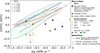 |
Fig. 3. [α/Fe] or [O/Fe] versus specific star formation rate in gas. Small filled diamonds represent [O/Fe] from GEAR (Revaz & Jablonka 2018; Roca-Fàbrega et al. 2021), which we fit with the solid blue line and a 3σ probability distribution function (blue shaded area). For comparison, the dashed brown and green curves, with corresponding contours, show [O/Fe] versus sSFR from the TNG100 (Chruślińska et al. 2024) and EAGLE (Matthee & Schaye 2018; Chruślińska et al. 2024) cosmological simulations, respectively. The measurements of [α/Fe] from absorption spectra of DLAs were taken from Velichko et al. (2024) (circles) and from Krogager et al. (2013), Fynbo et al. (2011), and Fynbo et al. (2013); we corrected the latter two for dust depletion (stars). The measurements of sSFRs were obtained by Møller & Christensen (2020), Christensen et al. (2014), Rahmati & Schaye (2014), Krogager et al. (2013), Fynbo et al. (2013), and Fynbo et al. (2011). The data for nearby galaxies (LMC, SMC, IZw 18, Sextans A, and NGC 3109) were taken from De Cia et al. (2024) and/or Chruślińska et al. (2024). All the abundances were converted to the Asplund et al. (2021) solar scale. |
The GEAR, TNG100, and EAGLE simulations show a slightly different behavior of [O/Fe] versus sSFR. In Fig. 3, galaxies evolve from the upper right to the bottom left corner. Early on, galaxies actively form stars, while their stellar masses are still quite low, and the α-element abundances are quite high because of the prevalence of CCSNe. With time, sSFR decreases, together with [α/Fe] caused by increasing contribution of SNe Ia.
Observed data for five DLA galaxies are shown by stars and circles in Fig. 3. The measurements of [α/Fe] obtained from absorption spectra of QSO-DLA sources and corrected for dust depletion were taken from Velichko et al. (2024). We also used the element abundances measured by Fynbo et al. (2013), Krogager et al. (2013), and Fynbo et al. (2011) from DLA spectra to calculate [α/Fe] corrected for dust depletion by applying the method from Velichko et al. (2024). The measurements of stellar masses and SFRs for the corresponding DLA counterparts were taken from Møller & Christensen (2020), Christensen et al. (2014), Rahmati & Schaye (2014), Krogager et al. (2013), Fynbo et al. (2013), and Fynbo et al. (2011). The data points for six nearby galaxies (LMC, SMC, IZw 18, Sextans A, and NGC 3109) shown by faint lozenges were taken from Chruślińska et al. (2024), where the values of [O/Fe] are obtained from emission-line diagnostics and the values of sSFRs calculated using the data from Skibba et al. (2012) for the SMC and LMC; Hunter et al. (2010) and/or Woo et al. (2008) for Sextans A and NGC 3109; Zhou et al. (2021) for IZw 18. We also included the values of [α/Fe] obtained by De Cia et al. (2024) from observations of gas in absorption in the SMC and LMC (triangles).
Most of the observed points are systematically lower than the relations predicted by the simulations. The factors behind these discrepancies in [α/Fe] likely differ according to the measurement specifics. (i) DLAs most often trace the outskirts of galaxies on scales of several tens of kiloparsecs and do not necessarily probe regions of recent star formation. Therefore, [α/Fe] observed in DLAs can be systematically lower than expected in simulated star-forming galaxies. (ii) The O and Fe measurements in nearby galaxies reported by Chruślińska et al. (2024) were based on different indicators; oxygen abundances were obtained using the direct gas-phase H II region–based method, while iron abundances in most cases (except for IZw 18) were determined from the spectra of young, bright stars such as blue or A-type supergiants. The emission-line diagnostics applied for this purpose can result in significant random and systematic uncertainties, so variations among different calibrations up to 0.7 dex were found (Kewley & Ellison 2008). Despite this, the values of [O/Fe] obtained by Chruślińska et al. (2024) are broadly consistent with the EAGLE simulations given the large uncertainties.
De Cia et al. (2024) employed a fundamentally different approach to studying the chemical composition of the ISM in the SMC and LMC, which is based on observations of the warm neutral medium in absorption. Using the “relative” method, the authors obtained the values of [α/Fe] corrected for dust depletion, which are higher than the [O/Fe] measurements from Chruślińska et al. (2024) by 0.52 and 0.41 dex for the SMC and LMC, respectively. The data reported by De Cia et al. (2024) are consistent with the simulations shown in Fig. 34.
Furthermore, the shape of the [O/Fe] versus sSFR relation was determined by a number of uncertain factors. Chruślińska et al. (2024) found that discrepancies between simulations are mainly attributed to the differences in the assumed SN Ia delay-time distribution and the relative SN Ia and CCSN formation efficiency and metal yields (which are the most difficult to set for the metal-poor CCSNe progenitors). The feedback model and other processes, such as merging and gas recycling, do not have a major effect on the average [O/Fe]–sSFR relation (Chruślińska et al. 2024). Constraining this relation with observational data is quite challenging because of large systematic errors (when using emission-line measurements) or incomparable observations (DLAs). The gamma-ray-burst (GRB) afterglows are expected to be more suitable to constrain the simulations than DLAs because the former probe the inner part of galaxies, but there are rarely enough abundance measurements to reliably obtain [α/Fe] according to Bolmer et al. (2019).
4.2. H I gas distribution
We applied the procedure described in Sect. 3.1 to all selected snapshots of the simulated galaxies, i.e., at redshifts 4.12, 3.49, 2.55, 2.01, 1.15, and 0.33. Fig. 4 shows column densities of H I averaged over 18 viewing angles versus galactocentric distances in the GEAR simulated galaxies taken at a redshift of 2.55. The shaded areas correspond to 1σ confidence intervals. The horizontal colored stripes in the background indicate intervals of the H I column density corresponding to DLA (20.3 cm−2 ≤ log N(H I) < 22 cm−2; Wolfe et al. 1986), sub-DLA (19 cm−2 ≤ log N(H I) < 20.3 cm−2)5, and Lyman-limit systems (17.2 cm−2 ≤ log N(H I) < 19 cm−2)6.
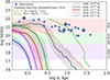 |
Fig. 4. H I column densities versus impact parameter at z > 1.9. Solid curves and 1σ confidence area correspond to the GEAR simulations (Revaz & Jablonka 2018; Roca-Fàbrega et al. 2021) at z = 2.55 averaged over 18 viewing angles. Blue diamonds show high-z observations from Christensen et al. (2014) and Møller & Christensen (2020), and compilations of observed data by Rahmati & Schaye (2014) and Krogager & Noterdaeme (2020). The highlighted symbols show the objects belonging to the golden sample from Velichko et al. (2024). Dashed curves show the data from hydrodynamical simulations performed with the use of the GADGET-3 code by Rahmati & Schaye (2014) in the stellar mass ranges of 7.0 < log(M★/M⊙) < 8.5 (orange) and 10.0 < log(M★/M⊙) < 11.5 (green). The horizontal colored stripes indicate intervals of the H I column density corresponding to DLA, sub-DLA, and Ly-limit systems (see text for details). |
Masses and/or impact parameters of four galaxies, corresponding to DLAs, which we studied in Velichko et al. (2024) – Q0528−250b, Q2206−199a, Q2243−605, and Q1135−0010 – were measured in the works of Christensen et al. (2014) and Møller & Christensen (2020). The data are summarized in Table 1 and highlighted in Fig. 4.
We see in Fig. 4 that the DLA size increases with the galaxy mass. As expected, the most massive GEAR galaxy h000 contains more gas, so its DLA size (∼4 kpc) is bigger than that of dwarf galaxies (< 2 kpc). Note that it has less gas in its center compared to less massive galaxies due to a merging event it underwent at z = 2.55, so the gas distribution was perturbed. For the least massive galaxy h074 with the stellar mass of 106.1 M⊙, even in the central part the gas is not dense enough for the galaxy to appear as a DLA. Thus, we established the lower stellar mass limit for the galaxies responsible for DLAs to be ∼106.5 M⊙ at z = 2.55. Compared to observations of high-z (z > 1.9) DLA counterparts from Christensen et al. (2014), Rahmati & Schaye (2014), Møller & Christensen (2020), and Krogager & Noterdaeme (2020) shown by blue diamonds, the gas in the GEAR simulations is not extended enough to reproduce the measured values. Strawn et al. (2024) also analyzed the galaxy h000 using Trident. However, they focused on the highly ionized gas in the circumgalactic medium, and therefore their results are not directly comparable to ours. In Fig. 4, we also show the data obtained from the hydrodynamical simulations performed by Rahmati & Schaye (2014) with the use of the GADGET-3 code in the stellar mass ranges of 7.0 < log(M★/M⊙) < 8.5 and 10.0 < log(M★/M⊙) < 11.5 shown by the dashed orange and green curves, respectively. Rahmati & Schaye (2014) used a different approach to searching for simulated DLA counterparts, according to which the HI absorbers associated with surrounding galaxies are linked to the main galaxy.
There is an overall agreement between the Rahmati & Schaye (2014) simulated DLAs and the observations. This may suggest that DLAs with large impact parameters may also be associated with surrounding galaxies (and they may have multiple counterparts). On the other hand, Rahmati & Schaye (2014) also found – when restricted to galaxies within the range of masses and star formation of detected DLA counterparts – similar impact parameters. Another important aspect to consider is that observed DLA counterparts are biased against small galaxies, which are typically too close in projection to the background QSO to be detected.
In Fig. 5, we compare the H I column density distribution for h000 at z = 0.33 with those from the AURIGA and TNG50 hydrodynamical simulations at a z of about zero. The blue curve shows the median 2D radial profile of log N(H I) for AURIGA galaxies at z = 0 − 0.3, with a stellar mass of log M★ = 10.7 M⊙ obtained by van de Voort et al. (2019). The stellar mass of the AURIGA galaxy is comparable to that of h000, but the gas is more extended, leading to its DLA size to be ten times larger: ∼30 kpc (AURIGA) versus ∼3 kpc (h000). Note that the central H I column densities in these two galaxies coincide. The green curve shows the cumulative covering fractions of H I from the post-processed TNG50 simulations of a galaxy with log M★ = 11.8 M⊙ at z = 0.5 (Nelson et al. 2020). It is an order of magnitude more massive than the AURIGA galaxy, but their DLA sizes coincide within their confidence intervals.
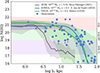 |
Fig. 5. H I column densities versus impact parameter at z ∼ 0. Gray curve: the GEAR galaxy h000 (log M★ = 10.8 M⊙ Roca-Fàbrega et al. 2021) taken at z = 0.33. Blue curve: median 2D radial profile of log N(H I) for an AURIGA galaxy at z = 0 − 0.3 with a stellar mass of log M★ = 10.7 M⊙ resimulated by van de Voort et al. (2019). Green curve: Cumulative covering fractions of H I from the TNG50 simulations of a galaxy with log M★ = 11.8 M⊙ (Nelson et al. 2020). The low-z observations taken from Christensen et al. (2014), Møller & Christensen (2020), Kulkarni et al. (2022), Weng et al. (2023), and Berg et al. (2023) are shown by blue diamonds. |
The values measured from observations in emission of DLA counterparts by Christensen et al. (2014), Kulkarni et al. (2022), and Møller & Christensen (2020) are also provided in Fig. 5. Most sources were detected at impact parameters higher than predicted even for the most massive GEAR galaxy h000. Unlike the TNG and Auriga models, the GEAR galaxy h000 has a highly concentrated center, which was also shown by Strawn et al. (2024). One of the reasons for this discrepancy includes the stellar feedback. Compared to TNG, Auriga, and EAGLE, GEAR has lower feedback coupling efficiency. The TNG and Auriga models explicitly generate outflows during stellar feedback events by forcing particles to exit the galaxy without hydrodynamical interaction (Grand et al. 2017; Pillepich et al. 2018). Similar outflows were obtained in EAGLE with the stochastic thermal feedback approach (Dalla Vecchia & Schaye 2012). These winds help in the removal of low-angular-momentum material, promoting the formation of more extended systems. On the contrary, GEAR employs thermal supernova feedback coupled with a delayed cooling phase (Stinson et al. 2006). While this scheme demonstrated to be sufficient to reproduce the stellar mass halo–mass relation for classical dwarfs (Revaz & Jablonka 2018), it does not lead to extended more massive systems. Another possible explanation lies in the ISM model. Unlike GEAR, the AURIGA and TNG50 models do not include the cooling of cold gas, which is artificially kept at a medium temperature of ∼104 K. Primarily, the AURIGA and TNG50 simulations reproduce the observed distribution of the absorbers with impact parameter more accurately because of accounting for satellite galaxies. This is consistent with the findings reported in Weng et al. (2024) for low-z objects that the central galaxy is only responsible for absorbers at the smallest impact parameters: b < 0.5 Rvir.
4.3. Velocities, masses, and metallicities
Figure E.1 shows the velocity width versus impact parameter in the five simulated galaxies (Revaz & Jablonka 2018; Roca-Fàbrega et al. 2021) z = 2.55. It increases with the galaxy mass, which is expected because, as mentioned in Sect. 2.2, Δv90 is a proxy for the galaxy dynamic mass. It also varies within the galaxies, gradually decreasing with impact parameter. We computed the mean and dispersion of velocity widths within DLA volumes of the simulated galaxies at each z, which allowed us to trace the changes of Δv90 on the stellar mass and metallicity of gas, as well as to investigate the mass–metallicity relation.
Compared to observations, velocity widths obtained within the simulated galaxies seem to be underestimated, especially in the outer parts of the galaxies, possibly due to insufficiently strong stellar feedback in the GEAR code, as mentioned in Sect. 4.2. On the other hand, the highest Δv90, measured in some DLAs can be overestimated because of significant contributions from components other than the rotational motion expected for their stellar masses from the stellar Tully–Fisher relation (sTFR) obtained in the work of Übler et al. (2017)7, which is shown in Fig. 6 by a gray line (see also the discussion in Arabsalmani et al. 2018). For example, in the case of the DLA counterpart detected by Christensen et al. (2014) (the green diamond highlighted in Fig. E.1), according to sTFR, its velocity width would only be 30% of the measured value if it were only due to rotation. The velocity spread obtained from gas observations in local galaxies, the LMC (∼100 km s−1, Poudel et al. 2025), and the SMC (∼90 km s−1, Murray et al. 2019), is roughly consistent with the Δv90 predicted by the GEAR simulations.
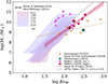 |
Fig. 6. Δv90 versus stellar mass. Filled areas correspond to the simulated data from Revaz & Jablonka (2018) and Roca-Fàbrega et al. (2021). Orange triangles show observations of GRBs used by Arabsalmani et al. (2018) to obtain the relation (dashed orange line). The observations of DLAs from Møller & Christensen (2020) are separated into low-z (≤0.1; magenta diamonds) and high-z (> 1.9; red diamonds) galaxies. The turquoise diamond shows observations of Christensen et al. (2014). The highlighted symbols correspond to the sources in the golden sample from Velichko et al. (2024). Red and blue lines with 95% confidence intervals show the linear fitting over high-z DLAs and high-z DLAs + GRBs subsamples, respectively. |
4.3.1. Δv90 versus stellar mass
In our previous work (Velichko et al. 2024), we used the Δv90 versus stellar mass relation obtained by Arabsalmani et al. (2018) based on observations of seven gamma-ray-burst (GRB)-selected galaxies (orange triangles and dashed orange fitting line in Fig. 6), and estimated that the Δv90 equal to 100 km s−1 (the breakpoint between low- and high-mass galaxies) corresponds to ∼109 M⊙. In this work, we tested this relation by comparing it with the simulated data and other observations, as shown in Fig. 6. The fitting line obtained by Arabsalmani et al. (2018) is inconsistent with both the simulations and observations of DLAs from Møller & Christensen (2020) and disk galaxies (Übler et al. 2017). Arabsalmani et al. (2018) assumed that galaxies with the highest Δv90 have significant contributions from components other than the rotational motion (as we discuss above). This leads to the fitting line obtained in their work being too shallow.
According to the data from Møller & Christensen (2020), the high-z DLAs (z > 1.9, red diamonds) tend to be systematically shifted toward higher Δv90 with respect to the low-z DLAs (z ≤ 1.9, magenta diamonds), which may indicate an evolution of the Δv90 versus M★ relation with redshift. This is consistent with the GEAR simulated data and can be explained by the fact that at higher redshift galaxies appear to be more turbulent. The fraction of interacting objects may also be higher. Compared to the orange trend from Arabsalmani et al. (2018), fitting the high-z Møller & Christensen (2020) subsample (red curve) gives a slope that is more consistent with both the sTFR obtained by Übler et al. (2017) for massive star-forming disk galaxies and the GEAR simulated data.
4.3.2. Δv90 versus metallicity
The Δv90–metallicity relation (see Fig. 7) was discovered in the work of Ledoux et al. (2006) based on observations of 70 DLAs located at redshifts in the range of 1.7 < z < 4.3, and it is the consequence of an underlying mass–metallicity relation. The authors found a strong redshift evolution of the relation for the 1.7 < z < 2.43 and 2.43 < z < 4.3 subsamples (dashed and dash-dotted lines in Fig. 7, respectively). Due to the fact that metallicities [X/H] in Ledoux et al. (2006) were traced by volatile metals without taking into account dust depletion, we applied an offset in metallicity of +0.2 and +0.35 dex for the high- and low-z subsamples to roughly correct the data, based on the mean adjustments found in De Cia et al. (2016). The shaded areas show the relations obtained from the gas component in the GEAR simulated galaxies (Revaz & Jablonka 2018; Roca-Fàbrega et al. 2021) at six redshifts (marked by gray numbers). The diamonds correspond to the observations of DLAs at z ≤ 2.1 (violet diamonds) and z > 2.1 (green diamonds) from Velichko et al. (2024), where the metallicities were corrected for dust depletion, [M/H]tot, and velocity widths are taken from the literature.
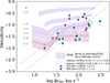 |
Fig. 7. Velocity widths versus metallicity relation. Shaded area: the simulated data from Revaz & Jablonka (2018) and Roca-Fàbrega et al. (2021) at six redshifts from z = 4.12 to 0.33 (numbers in gray), with vertical lines marking different models. Symbols show the data obtained from observations: total metallicities [M/H]tot corrected for dust depletion by Velichko et al. (2024) and Δv90 found in the literature in the redshift ranges z ≤ 2.1 (violet diamonds) and z > 2 (green diamonds). Gray lines show the best fit of data on 70 DLAs at redshifts of 1.7 < z < 2.43 (dashed line) and 2.43 < z < 4.3 (dash-dotted line) from Ledoux et al. (2006), biased in metallicity by +0.2 and +0.35 dex for the high- and low-z subsamples, respectively, to roughly take into account the dust depletion. |
There are some inconsistencies between the observations and simulations. First, at the low-Δv90 end, the simulated galaxies reach quite high metallicities that are not observed in real galaxies. The reasons for this could be that (i) these low-mass systems are simply missed in observation because the gas is not very extended, so, the probability of having a quasar in a line of sight crossing the gas is low, especially at low z; and (ii) the stellar feedback of the GEAR model is not strong enough, leading to slightly too-metal-rich systems. On the contrary, at the high-Δv90 end, model metallicities are not high enough to reproduce the slope that we expect from the observations (shown by the dashed gray line obtained by Ledoux et al. 2006). It is likely that GEAR may not be ideally calibrated in the MW-mass regime. Metallicity of gas in the galaxy h074 (with the lowest stellar mass and Δv90) is higher than in the more massive galaxy h050. This is possibly due to a slightly higher sSFR at the moment of formation of h074 compared to h050.
4.3.3. The mass–metallicity relation
The mass–(or luminosity) metallicity relation (MZR) has been known since the work of Lequeux et al. (1979). One possible explanation for its existence is that outflows, generated by starburst winds, blow metal-enriched gas out of low-mass galaxies more efficiently due to their shallower potential well, which slows down metal enrichment (Tremonti et al. 2004; De Lucia et al. 2004; Finlator & Davé 2008). Alternatively, the “galaxy downsizing” scenario has been proposed (Juneau et al. 2005; Feulner et al. 2005; Franceschini et al. 2006), according to which massive galaxies form most of their stars rapidly and at high redshifts, while low-mass galaxies evolve more slowly. Alternatively, Köppen et al. (2007) proposed a different mechanism for the origin of this dependence, which is based on a variation of the integrated galactic initial mass function on the SFR, which, in turn, varies in galaxies of different masses.
Mass–metallicity relations obtained from observations are mainly based on the gas-phase metallicity, which is traced by the oxygen abundance and usually quoted as 12+log(O/H). Fig. 8 compares the MZRs, with 12+log(O/H) being used as the metallicity tracer, obtained from the GEAR simulations at 0.33 ≤ z ≤ 4.12 (shaded bands of 1σ confidence intervals) with those obtained from observations of galaxies at different redshifts and mass ranges (colored curves). Here, we used the model abundance ratio O/H contained in the gas particles falling within DLA sizes of the GEAR galaxies.
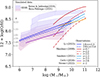 |
Fig. 8. Mass–metallicity relation using 12+log(O/H) as the metallicity tracer. Shaded bands: Simulated data with 1σ confidence intervals (Revaz & Jablonka 2018; Roca-Fàbrega et al. 2021) at redshifts marked by the numbers in gray. The curves present the observed MZR obtained in the literature. Dark blue: Li et al. (2023) values from the study of dwarf galaxies at 1.8 < z < 2.3 and 2.65 < z < 3.4 with JWST/NIRISS. Red: Maiolino et al. (2008) values found by reprocessing the data from Tremonti et al. (2004), Kewley & Ellison (2008), Savaglio et al. (2005), and Erb et al. (2006) at 0.1 < z < 2.2; as well as from the VLT near-IR observations performed with SINFONI at redshifts of 3 < z < 5. Blue: Sanders et al. (2021) values from the MOSDEF survey of galaxies at z ∼ 2.3 and 3.3. Purple: Curti et al. (2024) values from the analysis of low-mass galaxies at 3 < z < 6 observed with JWST/NIRSpec. Orange: Strom et al. (2022) values from a sample of 195 star-forming galaxies at z ∼ 2 from the Keck Baryonic Structure Survey. |
Maiolino et al. (2008) found a strong evolution of MZR with redshift (at 0.1 < z < 5) in the galaxy mass range of 8.5 < M★/M⊙ < 11 by collecting and reprocessing data from Tremonti et al. (2004) and Kewley & Ellison (2008) at z ∼ 0.1; from Savaglio et al. (2005) at 0.4 < z < 1; and from Erb et al. (2006) at z ∼ 2.2; as well as from the new near-IR observations of galaxies at 3 < z < 5 performed at the VLT with SINFONI (see red curves in Fig. 8). Sanders et al. (2021) investigated the MZRs using representative samples of ∼300 galaxies at z ∼ 2.3 and ∼150 galaxies at z ∼ 3.3 from the MOSDEF survey (Kriek et al. 2015), a program that used the Multi-Object Spectrometer For Infrared Exploration (MOSFIRE, McLean et al. 2012). From these data, the evolution with redshift is less prominent than it was when obtained by Maiolino et al. (2008), and the slope is shallower (blue curves in Fig. 8). Strom et al. (2022) obtained an even shallower slope from a sample of 195 star-forming galaxies at z ∼ 2 from the Keck Baryonic Structure Survey (orange curve in Fig. 8). In the low-mass regime (M★/M⊙ < 9.5), the MZRs were obtained in the works of Li et al. (2023), which used observations of 51 dwarf galaxies at z = 2 − 3 from JWST/NIRISS imaging and slitless grism spectroscopic observations (dark blue curves in Fig. 8), and Curti et al. (2024), based on observations of galaxies at 3 < z < 6 with JWST/NIRSpec (purple curve in Fig. 8).
Overall, observations of distant galaxies show some variations in the behavior of the MZR and its dependence on redshift. The evolution with redshift noted in the works of Li et al. (2023) and Sanders et al. (2021) is smaller compared to that of the GEAR simulations. To simplify the comparison, from the data displayed in Fig. 8, we only select those corresponding to z ∼ 2 (see Fig. 9). We added the MZR obtained by Torrey et al. (2019) from the TNG100 simulations at z = 2 (the shaded green band of the 1σ confidence interval in Fig. 9). Although the extent of the gas distribution might be underestimated by GEAR (see the discussion in Sect. 4.2), the chemical modeling is robust and also consistent with the TNG100 simulations. GEAR is particularly important, because it constrains the MZR in the low-mass range, which is not targeted by such projects as Illustris-TNG and AURIGA. Despite some differences in slopes, the MZRs obtained from observations by Li et al. (2023) and Sanders et al. (2021), and Strom et al. (2022) are in agreement with the simulations within 1σ confidence intervals. The slope obtained by Maiolino et al. (2008) is steeper than both simulations and other observations.
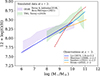 |
Fig. 9. Mass–metallicity relation at z ∼ 2. Blue shaded area: Simulated data from Revaz & Jablonka (2018) and Roca-Fàbrega et al. (2021) at z = 2.01. Green shaded area: MZR obtained by Torrey et al. (2019) from the TNG simulations at z = 2. The colored curves present the observed MZR obtained in the literature at z ∼ 2 (the same line styles as in Fig. 8). |
5. Conclusions
In this work, we conducted a comprehensive comparison of chemical and dynamical properties of DLA galaxies studied in Velichko et al. (2024), Weng et al. (2023), Berg et al. (2023), Kulkarni et al. (2022), Møller & Christensen (2020), Christensen et al. (2014), Rahmati & Schaye (2014), Krogager et al. (2013), Fynbo et al. (2013), and Fynbo et al. (2011) with the chemodynamical GEAR simulations performed by Revaz & Jablonka (2018) and Roca-Fàbrega et al. (2021) that cover the stellar mass range of 6.1 ≤ M★/M⊙ ≤ 10.8 and redshifts from 4.12 to 0.33. We additionally incorporated chemodynamical properties of model galaxies obtained from the Illustris-TNG (Nelson et al. 2020), EAGLE (Matthee & Schaye 2018), AURIGA (van de Voort et al. 2019), and modified OWL simulations (Rahmati & Schaye 2014).
We find that the abundance ratios [α/Fe] and [M/H] observed in the ISM of DLA galaxies almost completely overlap with the abundance trends in gas of the simulated galaxies. From Fig. 2, we conclude that the DLA galaxies in our sample from Velichko et al. (2024) may be associated with stellar mass ranges of 106 − 108 M⊙ and of 108 − 1011 M⊙ for the low- and high-Δv90 subsamples, respectively. The simulated galaxies also confirm that the α knee is at lower metallicities for lower mass galaxies.
We confirm that high values of [α/Fe] trace intense recent star formation in galaxies (see Fig. 3). The GEAR, TNG100, and EAGLE simulations show a slightly different behavior of [O/Fe] versus sSFR, but all the relations are consistent within 3σ confidence areas. The discrepancies with the observations arise from different factors, depending on specifics such as the type of source and the abundance-determination method employed. We found good agreement between all the theoretical relations shown in Fig. 3 and the values of [α/Fe] determined by De Cia et al. (2024) for the LMC and SMC ISMs based on observations of the warm neutral medium in absorption. The rest observations are barely consistent with the model predictions; this is due to the likely presence of large systematic errors up to 0.7 dex (in case of observations in emission; Chruślińska et al. 2024; Kewley & Ellison 2008) or incomparable observations (DLA versus host galaxy; Rahmati & Schaye 2014; Weng et al. 2024).
We investigated the distribution of gas in the GEAR simulated galaxies (Fig. 4) and find that they are more compact than the observed DLAs. For example, in the MW-mass galaxy h000, the high-density gas corresponding to DLA is concentrated within ∼4 kpc, while the measured impact parameters of DLAs can be ten times larger. Considering that DLAs are commonly observed in group environments (e.g., Péroux et al. 2019), one of the ways to resolve the inconsistency is to search for high-density HI absorbers outside the main galaxy, which is supported in the work of Rahmati & Schaye (2014). Based on the TNG50 simulations, Weng et al. (2024) showed that only at low-z are the absorbers observed at impact parameters smaller than 0.5 Rvir associated with the central galaxy, and this value decreases with increasing column density. Otherwise, they predominantly arise from satellite and other halo galaxies. The smaller DLA galaxies cannot be detected in emission at small impact parameters, because they are too close in projection to the background QSO.
The GEAR simulations exhibit a systematic redshift evolution of the Δv90 – stellar mass relation toward lower Δv90, a trend corroborated by the observational data of Møller & Christensen (2020). However, constraining the slope of the relation remains a nontrivial issue: the GEAR data reproduce the sTFR obtained by Übler et al. (2017) well, while the slope obtained by fitting the data for high-z DLAs from Møller & Christensen (2020) is somewhat shallower, and incorporating the measurements from Christensen et al. (2014) and particularly the values obtained by Arabsalmani et al. (2018) from GRBs, further increases the discrepancy. The high-velocity widths, Δv90, obtained for the DLAs at high impact parameters (see also Fig. E.1), as well as GRBs (Arabsalmani et al. 2018), can be explained by contribution from components other than rotational motion; for example, multiple objects such as intergalactic clouds and/or satellite galaxies intersected by a DLA along an extended sightline (Rahmati & Schaye 2014; Weng et al. 2024). One of the main results is that the GEAR simulations also reproduce the most recently observed mass–metallicity relations at z ∼ 2 well (see Fig. 9).
Here, we compared our results with a small set of other simulated galaxies, attempting to (1) validate the GEAR simulations against other simulations, in a parameter space that is more relevant for DLAs; and (2) slightly extend the comparison to galaxy properties that are beyond those simulated with GEAR, to check for other potential limitations and improvements of GEAR simulations.
Overall, this is the first time we compared the chemodynamical properties of observed and simulated galaxies at z ∼ 2 − 4 in such detail. It is quite difficult to make simulations that would perfectly reproduce all the varieties of observed galaxy properties. The comprehensive analysis we performed in this work helps us better understand the processes governing the formation and evolution of galaxies. The results of this work consolidate the use of DLAs for the study of galaxy (chemical) evolution. A full and detailed analysis and discussion of the comparison with the additional simulations, beyond GEAR, as well as the exploration of the variation of the assumptions of GEAR simulations, in particular its feedback prescription, is beyond the scope of this study and should be addressed in future work.
Acknowledgments
A.V., A.D.C. and J.K.K. acknowledge support by the Swiss National Science Foundation under grant 185692 funding the “Interstellar One” project. J.K.K. acknowledges financial support from the French Agence Nationale de la Recherche (ANR) under grant number ANR-24-CE31-7454. We are grateful to the anonymous referee for valuable comments and suggestions, which significantly improved the manuscript.
References
- Altay, G., Theuns, T., Schaye, J., Booth, C. M., & Dalla Vecchia, C. 2013, MNRAS, 436, 2689 [NASA ADS] [CrossRef] [Google Scholar]
- Arabsalmani, M., Møller, P., Freudling, W., et al. 2016, IAU Focus Meeting, 29B, 263 [Google Scholar]
- Arabsalmani, M., Møller, P., Perley, D. A., et al. 2018, MNRAS, 473, 3312 [NASA ADS] [CrossRef] [Google Scholar]
- Asplund, M., Amarsi, A. M., & Grevesse, N. 2021, A&A, 653, A141 [NASA ADS] [CrossRef] [EDP Sciences] [Google Scholar]
- Berg, M. A., Lehner, N., Howk, J. C., et al. 2023, ApJ, 944, 101 [Google Scholar]
- Bolmer, J., Ledoux, C., Wiseman, P., et al. 2019, A&A, 623, A43 [NASA ADS] [CrossRef] [EDP Sciences] [Google Scholar]
- Calura, F., Pipino, A., Matteucci, F., et al. 2009, AIP Conf. Ser., 1111, 151 [Google Scholar]
- Cen, R. 2012, ApJ, 748, 121 [NASA ADS] [CrossRef] [Google Scholar]
- Chemerynska, I., Atek, H., Dayal, P., et al. 2024, ApJ, 976, L15 [NASA ADS] [CrossRef] [Google Scholar]
- Christensen, L., Møller, P., Fynbo, J. P. U., & Zafar, T. 2014, MNRAS, 445, 225 [NASA ADS] [CrossRef] [Google Scholar]
- Chruślińska, M., Pakmor, R., Matthee, J., & Matsuno, T. 2024, A&A, 686, A186 [NASA ADS] [CrossRef] [EDP Sciences] [Google Scholar]
- Curti, M., Maiolino, R., Curtis-Lake, E., et al. 2024, A&A, 684, A75 [NASA ADS] [CrossRef] [EDP Sciences] [Google Scholar]
- Dalla Vecchia, C., & Schaye, J. 2012, MNRAS, 426, 140 [NASA ADS] [CrossRef] [Google Scholar]
- de Boer, T. J. L., Belokurov, V., Beers, T. C., & Lee, Y. S. 2014, MNRAS, 443, 658 [NASA ADS] [CrossRef] [Google Scholar]
- De Cia, A., Ledoux, C., Mattsson, L., et al. 2016, A&A, 596, A97 [NASA ADS] [CrossRef] [EDP Sciences] [Google Scholar]
- De Cia, A., Roman-Duval, J., Konstantopoulou, C., et al. 2024, A&A, 683, A216 [NASA ADS] [CrossRef] [EDP Sciences] [Google Scholar]
- De Lucia, G., Kauffmann, G., & White, S. D. M. 2004, MNRAS, 349, 1101 [Google Scholar]
- Djorgovski, S. G., Pahre, M. A., Bechtold, J., & Elston, R. 1996, Nature, 382, 234 [NASA ADS] [CrossRef] [Google Scholar]
- Erb, D. K., Steidel, C. C., Shapley, A. E., et al. 2006, ApJ, 646, 107 [NASA ADS] [CrossRef] [Google Scholar]
- Faucher-Giguère, C.-A., Hopkins, P. F., Kereš, D., et al. 2015, MNRAS, 449, 987 [CrossRef] [Google Scholar]
- Feulner, G., Gabasch, A., Salvato, M., et al. 2005, ApJ, 633, L9 [NASA ADS] [CrossRef] [Google Scholar]
- Finlator, K., & Davé, R. 2008, MNRAS, 385, 2181 [NASA ADS] [CrossRef] [Google Scholar]
- Fontana, A., Salimbeni, S., Grazian, A., et al. 2006, A&A, 459, 745 [CrossRef] [EDP Sciences] [Google Scholar]
- Franceschini, A., Rodighiero, G., Cassata, P., et al. 2006, A&A, 453, 397 [NASA ADS] [CrossRef] [EDP Sciences] [Google Scholar]
- Fumagalli, M., Prochaska, J. X., Kasen, D., et al. 2011, MNRAS, 418, 1796 [CrossRef] [Google Scholar]
- Fynbo, J. P. U., Prochaska, J. X., Sommer-Larsen, J., Dessauges-Zavadsky, M., & Møller, P. 2008, ApJ, 683, 321 [NASA ADS] [CrossRef] [Google Scholar]
- Fynbo, J. P. U., Ledoux, C., Noterdaeme, P., et al. 2011, MNRAS, 413, 2481 [CrossRef] [Google Scholar]
- Fynbo, J. P. U., Geier, S. J., Christensen, L., et al. 2013, MNRAS, 436, 361 [CrossRef] [Google Scholar]
- Garratt-Smithson, L., Power, C., Lagos, C. D. P., et al. 2021, MNRAS, 501, 4396 [Google Scholar]
- Grand, R. J. J., Gómez, F. A., Marinacci, F., et al. 2017, MNRAS, 467, 179 [NASA ADS] [Google Scholar]
- Haardt, F., & Madau, P. 2012, ApJ, 746, 125 [Google Scholar]
- Haehnelt, M. G., Steinmetz, M., & Rauch, M. 1998, ApJ, 495, 647 [NASA ADS] [CrossRef] [Google Scholar]
- Hassan, S., Finlator, K., Davé, R., Churchill, C. W., & Prochaska, J. X. 2020, MNRAS, 492, 2835 [Google Scholar]
- Hasselquist, S., Hayes, C. R., Lian, J., et al. 2021, ApJ, 923, 172 [NASA ADS] [CrossRef] [Google Scholar]
- Henry, A., Rafelski, M., Sunnquist, B., et al. 2021, ApJ, 919, 143 [NASA ADS] [CrossRef] [Google Scholar]
- Hummels, C. B., Bryan, G. L., Smith, B. D., & Turk, M. J. 2013, MNRAS, 430, 1548 [NASA ADS] [CrossRef] [Google Scholar]
- Hummels, C. B., Smith, B. D., & Silvia, D. W. 2017, ApJ, 847, 59 [Google Scholar]
- Hunter, D. A., Elmegreen, B. G., & Ludka, B. C. 2010, AJ, 139, 447 [NASA ADS] [CrossRef] [Google Scholar]
- Jedamzik, K., & Prochaska, J. X. 1998, MNRAS, 296, 430 [Google Scholar]
- Juneau, S., Glazebrook, K., Crampton, D., et al. 2005, ApJ, 619, L135 [NASA ADS] [CrossRef] [Google Scholar]
- Kashino, D., Lilly, S. J., Renzini, A., et al. 2022, ApJ, 925, 82 [NASA ADS] [CrossRef] [Google Scholar]
- Katz, N. 1992, ApJ, 391, 502 [NASA ADS] [CrossRef] [Google Scholar]
- Katz, N., Weinberg, D. H., & Hernquist, L. 1996, ApJS, 105, 19 [NASA ADS] [CrossRef] [Google Scholar]
- Kewley, L. J., & Ellison, S. L. 2008, ApJ, 681, 1183 [Google Scholar]
- Kim, J.-H., Agertz, O., Teyssier, R., et al. 2016, ApJ, 833, 202 [NASA ADS] [CrossRef] [Google Scholar]
- Klimenko, V. V., Kulkarni, V., Wake, D. A., et al. 2023, ApJ, 954, 115 [Google Scholar]
- Kobayashi, C., Tsujimoto, T., & Nomoto, K. 2000, ApJ, 539, 26 [NASA ADS] [CrossRef] [Google Scholar]
- Kobayashi, C., Karakas, A. I., & Lugaro, M. 2020, ApJ, 900, 179 [Google Scholar]
- Köppen, J., Weidner, C., & Kroupa, P. 2007, MNRAS, 375, 673 [CrossRef] [Google Scholar]
- Kriek, M., Shapley, A. E., Reddy, N. A., et al. 2015, ApJS, 218, 15 [NASA ADS] [CrossRef] [Google Scholar]
- Krogager, J.-K., & Noterdaeme, P. 2020, A&A, 644, L6 [NASA ADS] [CrossRef] [EDP Sciences] [Google Scholar]
- Krogager, J.-K., Fynbo, J. P. U., Ledoux, C., et al. 2013, MNRAS, 433, 3091 [NASA ADS] [CrossRef] [Google Scholar]
- Krogager, J. K., Møller, P., Fynbo, J. P. U., & Noterdaeme, P. 2017, MNRAS, 469, 2959 [NASA ADS] [CrossRef] [Google Scholar]
- Kulkarni, V. P., Bowen, D. V., Straka, L. A., et al. 2022, ApJ, 929, 150 [Google Scholar]
- Ledoux, C., Petitjean, P., Fynbo, J. P. U., Møller, P., & Srianand, R. 2006, A&A, 457, 71 [NASA ADS] [CrossRef] [EDP Sciences] [Google Scholar]
- Lequeux, J., Peimbert, M., Rayo, J. F., Serrano, A., & Torres-Peimbert, S. 1979, A&A, 80, 155 [Google Scholar]
- Li, M., Cai, Z., Bian, F., et al. 2023, ApJ, 955, L18 [CrossRef] [Google Scholar]
- Liang, C. J., Kravtsov, A. V., & Agertz, O. 2016, MNRAS, 458, 1164 [CrossRef] [Google Scholar]
- Ma, J., Ge, J., Lundgren, B. F., & Prochaska, J. X. 2015, Revealing the Host Galaxy of a Strong Milky Way-type 2175 Angstrom Absorber at z = 2.12, HST Proposal. Cycle 23 [Google Scholar]
- Maiolino, R., Nagao, T., Grazian, A., et al. 2008, A&A, 488, 463 [NASA ADS] [CrossRef] [EDP Sciences] [Google Scholar]
- Maller, A. H., Prochaska, J. X., Somerville, R. S., & Primack, J. R. 2001, MNRAS, 326, 1475 [Google Scholar]
- Matteucci, F. 2012, Chemical Evolution of Galaxies (Berlin Heidelberg: Springer-Verlag) [Google Scholar]
- Matthee, J., & Schaye, J. 2018, MNRAS, 479, L34 [NASA ADS] [Google Scholar]
- McLean, I. S., Steidel, C. C., Epps, H. W., et al. 2012, SPIE Conf. Ser., 8446, 84460J [NASA ADS] [Google Scholar]
- McWilliam, A. 1997, ARA&A, 35, 503 [NASA ADS] [CrossRef] [Google Scholar]
- Møller, P., & Christensen, L. 2020, MNRAS, 492, 4805 [CrossRef] [Google Scholar]
- Møller, P., Warren, S. J., Fall, S. M., Fynbo, J. U., & Jakobsen, P. 2002, ApJ, 574, 51 [CrossRef] [Google Scholar]
- Murray, C. E., Peek, J. E. G., Di Teodoro, E. M., et al. 2019, ApJ, 887, 267 [Google Scholar]
- Nagamine, K., Wolfe, A. M., Hernquist, L., & Springel, V. 2007, ApJ, 660, 945 [Google Scholar]
- Nelson, D., Sharma, P., Pillepich, A., et al. 2020, MNRAS, 498, 2391 [NASA ADS] [CrossRef] [Google Scholar]
- Oppenheimer, B. D., Davé, R., Katz, N., Kollmeier, J. A., & Weinberg, D. H. 2012, MNRAS, 420, 829 [NASA ADS] [CrossRef] [Google Scholar]
- Oppenheimer, B. D., Crain, R. A., Schaye, J., et al. 2016, MNRAS, 460, 2157 [NASA ADS] [CrossRef] [Google Scholar]
- Péroux, C., Zwaan, M. A., Klitsch, A., et al. 2019, MNRAS, 485, 1595 [CrossRef] [Google Scholar]
- Péroux, C., Nelson, D., van de Voort, F., et al. 2020, MNRAS, 499, 2462 [CrossRef] [Google Scholar]
- Pillepich, A., Springel, V., Nelson, D., et al. 2018, MNRAS, 473, 4077 [Google Scholar]
- Pontzen, A., Governato, F., Pettini, M., et al. 2008, MNRAS, 390, 1349 [NASA ADS] [Google Scholar]
- Poudel, S., Horton, A., Vazquez, J., et al. 2025, ApJ, 984, 161 [Google Scholar]
- Prochaska, J. X., & Herbert-Fort, S. 2004, PASP, 116, 622 [NASA ADS] [CrossRef] [Google Scholar]
- Prochaska, J. X., & Wolfe, A. M. 1997, ApJ, 487, 73 [NASA ADS] [CrossRef] [Google Scholar]
- Rahmati, A., & Schaye, J. 2014, MNRAS, 438, 529 [NASA ADS] [CrossRef] [Google Scholar]
- Rahmati, A., Pawlik, A. H., Raičević, M., & Schaye, J. 2013, MNRAS, 430, 2427 [NASA ADS] [CrossRef] [Google Scholar]
- Revaz, Y. 2013, Astrophysics Source Code Library [record ascl:1302.004] [Google Scholar]
- Revaz, Y., & Jablonka, P. 2012, A&A, 538, A82 [CrossRef] [EDP Sciences] [Google Scholar]
- Revaz, Y., & Jablonka, P. 2018, A&A, 616, A96 [NASA ADS] [CrossRef] [EDP Sciences] [Google Scholar]
- Revaz, Y., Arnaudon, A., Nichols, M., Bonvin, V., & Jablonka, P. 2016, A&A, 588, A21 [NASA ADS] [CrossRef] [EDP Sciences] [Google Scholar]
- Rhodin, N. H. P., Agertz, O., Christensen, L., Renaud, F., & Fynbo, J. P. U. 2019, MNRAS, 488, 3634 [NASA ADS] [CrossRef] [Google Scholar]
- Roca-Fàbrega, S., Kim, J.-H., Hausammann, L., et al. 2021, ApJ, 917, 64 [CrossRef] [Google Scholar]
- Sanders, R. L., Shapley, A. E., Jones, T., et al. 2021, ApJ, 914, 19 [CrossRef] [Google Scholar]
- Saro, A., Mohr, J. J., Bazin, G., & Dolag, K. 2013, ApJ, 772, 47 [NASA ADS] [CrossRef] [Google Scholar]
- Savaglio, S., Glazebrook, K., Le Borgne, D., et al. 2005, AIP Conf. Ser., 761, 425 [Google Scholar]
- Schaye, J., Dalla Vecchia, C., Booth, C. M., et al. 2010, MNRAS, 402, 1536 [Google Scholar]
- Scholte, D., Saintonge, A., Moustakas, J., et al. 2024, MNRAS, 535, 2341 [Google Scholar]
- Shen, S., Madau, P., Aguirre, A., et al. 2012, ApJ, 760, 50 [NASA ADS] [CrossRef] [Google Scholar]
- Shen, S., Madau, P., Guedes, J., et al. 2013, ApJ, 765, 89 [NASA ADS] [CrossRef] [Google Scholar]
- Skibba, R. A., Engelbracht, C. W., Aniano, G., et al. 2012, ApJ, 761, 42 [NASA ADS] [CrossRef] [Google Scholar]
- Smith, B. D., Bryan, G. L., Glover, S. C. O., et al. 2017, MNRAS, 466, 2217 [NASA ADS] [CrossRef] [Google Scholar]
- Springel, V., & Hernquist, L. 2003, MNRAS, 339, 289 [Google Scholar]
- Stinson, G., Seth, A., Katz, N., et al. 2006, MNRAS, 373, 1074 [NASA ADS] [CrossRef] [Google Scholar]
- Stinson, G. S., Brook, C., Prochaska, J. X., et al. 2012, MNRAS, 425, 1270 [NASA ADS] [CrossRef] [Google Scholar]
- Strawn, C., Roca-Fàbrega, S., Primack, J. R., et al. 2024, ApJ, 962, 29 [Google Scholar]
- Strom, A. L., Rudie, G. C., Steidel, C. C., & Trainor, R. F. 2022, ApJ, 925, 116 [NASA ADS] [CrossRef] [Google Scholar]
- Tinsley, B. M. 1979, ApJ, 229, 1046 [Google Scholar]
- Tinsley, B. M. 1980, Fund. Cosmic Phys., 5, 287 [Google Scholar]
- Tolstoy, E., Hill, V., & Tosi, M. 2009, ARA&A, 47, 371 [Google Scholar]
- Torrey, P., Vogelsberger, M., Marinacci, F., et al. 2019, MNRAS, 484, 5587 [NASA ADS] [Google Scholar]
- Tremonti, C. A., Heckman, T. M., Kauffmann, G., et al. 2004, ApJ, 613, 898 [Google Scholar]
- Tsujimoto, T., Nomoto, K., Yoshii, Y., et al. 1995, MNRAS, 277, 945 [Google Scholar]
- Übler, H., Förster Schreiber, N. M., Genzel, R., et al. 2017, ApJ, 842, 121 [Google Scholar]
- van de Voort, F., Springel, V., Mandelker, N., van den Bosch, F. C., & Pakmor, R. 2019, MNRAS, 482, L85 [NASA ADS] [CrossRef] [Google Scholar]
- Velichko, A., De Cia, A., Konstantopoulou, C., et al. 2024, A&A, 685, A103 [NASA ADS] [CrossRef] [EDP Sciences] [Google Scholar]
- Weng, S., Péroux, C., Karki, A., et al. 2023, MNRAS, 519, 931 [Google Scholar]
- Weng, S., Péroux, C., Ramesh, R., et al. 2024, MNRAS, 527, 3494 [Google Scholar]
- Wolfe, A. M., Turnshek, D. A., Smith, H. E., & Cohen, R. D. 1986, ApJS, 61, 249 [NASA ADS] [CrossRef] [Google Scholar]
- Wolfe, A. M., Lanzetta, K. M., Foltz, C. B., & Chaffee, F. H. 1995, ApJ, 454, 698 [Google Scholar]
- Wolfe, A. M., Gawiser, E., & Prochaska, J. X. 2005, ARA&A, 43, 861 [NASA ADS] [CrossRef] [Google Scholar]
- Woo, J., Courteau, S., & Dekel, A. 2008, MNRAS, 390, 1453 [NASA ADS] [Google Scholar]
- Worthey, G., Faber, S. M., & Gonzalez, J. J. 1992, ApJ, 398, 69 [Google Scholar]
- Zhou, L., Shi, Y., Zhang, Z.-Y., & Wang, J. 2021, A&A, 653, L10 [NASA ADS] [CrossRef] [EDP Sciences] [Google Scholar]
There are some exceptions: lensing, SNe, GRBs, and so on.
We test this relation in Sect. 4.3.1.
We note that although our focus was on issues related to abundance determinations, uncertainties also exist in the measurements of SFR and M★. These include, among other factors, systematic effects arising from the choice of SFR tracer, the assumed IMF, applied dust corrections, and the stellar population synthesis model used in certain stellar mass estimation methods (Chruślińska et al. 2024).
According to the nomenclature of Prochaska & Herbert-Fort (2004), these systems are called “super-Lyman-limit systems” (SLLSs).
The systems with log N(H I) < 17.2 cm−2 are referred to as Lyman-α forest absorbers.
According to the data from Übler et al. (2017), sTFR is log M★ = 3.56 log Vcirc + 2.25.
Appendix A: Additional details of the GEAR galaxies
Some characteristics of the GEAR galaxies are provided in Table A.1. Fig. A.1 shows the evolution of stellar and gas masses (measured within the virial radius Rvir) of the galaxies with redshift. The number of stars gradually increases with the galaxy evolution due to star formation processes, while the amount of gas on average gradually decreases because one part of the gas transforms into stars, another is ejected due to outflows caused by stellar feedback and UV-background heating during the reionization epoch (Revaz & Jablonka 2018). This effect is especially important for the least massive galaxy h074 with shallower potential well (blue curves in Fig. A.1), which quickly loses almost all its gas by z = 0.33. On the other hand, the gas reservoirs can also be replenished through gas accretion and/or merger events. For example, the gray solid curve in Fig. A.1, corresponding to the h000 galaxy, shows a slight increase in the mass of gas between z = 2.55 and 2.01 because of merging, which is consistent with the results shown in Fig. 2 of Strawn et al. (2024). The gas fraction fgas = Mgas/(Mgas + M★) gradually decreases with galaxy evolution, as shown in Fig. A.2, but the four more massive galaxies remain gas-rich systems (with fgas ≥ 50%) down to z ∼ 1, while in the h074 galaxy fgas decreases sharply starting from z ∼ 2 and reaches 0% by z = 0 due to more efficient gas loss.
Properties of the GEAR galaxies at z = 0.
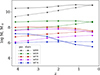 |
Fig. A.1. Redshift evolution of stellar and gas masses measured within Rvir in the five simulated galaxies. The solid and dashed curves correspond to the gas and stellar components, respectively. |
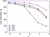 |
Fig. A.2. Fraction of all gas in the simulated galaxies Mgas/(Mgas + M★). |
Appendix B: An illustration of a DLA
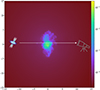 |
Fig. B.1. Illustration of a line-of-sight passing through the simulated galaxy h026 taken at z = 2.01. The schematic image of a quasar is taken from the © NASA image gallery. |
Appendix C: Determination of Δv90
List of lines used to determine Δv90.
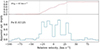 |
Fig. C.1. Measurement of the velocity width Δv90 of the absorption line profile of Fe II λ1125 in the mock spectrum for the galaxy h026 taken at z = 2.01. The spectrum is obtained along the line of sight at an impact parameter b = 1.5 kpc. Upper panel: normalized total apparent optical depth, the dashed vertical lines show the velocity range between 5% and 95% of the total apparent optical depth (lower panel). The resulting Δv90 is 61 km s−1. |
Appendix D: Specific star formation rates in the simulated galaxies
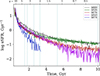 |
Fig. D.1. The sSFR vs. time for the GEAR galaxies from Revaz & Jablonka (2018) and Roca-Fàbrega et al. (2021). The vertical lines mark the six redshifts z = 4.12, 3.49, 2.55, 2.01, 1.15, 0.33 at which we take the model galaxies. |
Appendix E: Velocity widths
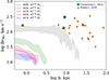 |
Fig. E.1. Velocity widths vs. impact parameter in the simulated galaxies at z = 2.55 compared to the data obtained from observations in emission by Christensen et al. (2014) (orange triangles) and Møller & Christensen (2020) (green diamonds). The highlighted symbols correspond to the systems studied in Velichko et al. (2024) (see Table 1). |
All Tables
All Figures
|
Fig. 1. The surface density of all gas for the five GEAR galaxies (Revaz & Jablonka 2018; Roca-Fàbrega et al. 2021) at redshifts 4.12 (upper panel) and 0.33 (lower panel). For h074, the lower rightmost panel is empty, as all the gas has been removed by photoevaporation. |
| In the text | |
|
Fig. 2. [α/Fe] versus metallicity. Shaded area: [Mg/Fe] versus [Fe/H] in gas of five simulated galaxies h000, h026, h076, h050, and h074 at z from 4.12 to 0.33 (see the numbers). In the case of h074, there were no gas particles left at z < 2.01. Open orange diamonds and open blue triangles show the values [α/Fe]nucl obtained by Velichko et al. (2024) from the observations of the ISM in QSO-DLAs in the high- and low-Δv90 subsamples, respectively. Filled symbols mark DLAs masses determined by Møller & Christensen (2020) or Christensen et al. (2014) from observations in emission of the DLA counterparts (see Table 1). The blue and orange curves are three-piecewise fits to the data for the low- and high-Δv90 subsamples obtained in Velichko et al. (2024). The dashed gray curve shows the α-element enhancements obtained for the MW by McWilliam (1997). |
| In the text | |
|
Fig. 3. [α/Fe] or [O/Fe] versus specific star formation rate in gas. Small filled diamonds represent [O/Fe] from GEAR (Revaz & Jablonka 2018; Roca-Fàbrega et al. 2021), which we fit with the solid blue line and a 3σ probability distribution function (blue shaded area). For comparison, the dashed brown and green curves, with corresponding contours, show [O/Fe] versus sSFR from the TNG100 (Chruślińska et al. 2024) and EAGLE (Matthee & Schaye 2018; Chruślińska et al. 2024) cosmological simulations, respectively. The measurements of [α/Fe] from absorption spectra of DLAs were taken from Velichko et al. (2024) (circles) and from Krogager et al. (2013), Fynbo et al. (2011), and Fynbo et al. (2013); we corrected the latter two for dust depletion (stars). The measurements of sSFRs were obtained by Møller & Christensen (2020), Christensen et al. (2014), Rahmati & Schaye (2014), Krogager et al. (2013), Fynbo et al. (2013), and Fynbo et al. (2011). The data for nearby galaxies (LMC, SMC, IZw 18, Sextans A, and NGC 3109) were taken from De Cia et al. (2024) and/or Chruślińska et al. (2024). All the abundances were converted to the Asplund et al. (2021) solar scale. |
| In the text | |
|
Fig. 4. H I column densities versus impact parameter at z > 1.9. Solid curves and 1σ confidence area correspond to the GEAR simulations (Revaz & Jablonka 2018; Roca-Fàbrega et al. 2021) at z = 2.55 averaged over 18 viewing angles. Blue diamonds show high-z observations from Christensen et al. (2014) and Møller & Christensen (2020), and compilations of observed data by Rahmati & Schaye (2014) and Krogager & Noterdaeme (2020). The highlighted symbols show the objects belonging to the golden sample from Velichko et al. (2024). Dashed curves show the data from hydrodynamical simulations performed with the use of the GADGET-3 code by Rahmati & Schaye (2014) in the stellar mass ranges of 7.0 < log(M★/M⊙) < 8.5 (orange) and 10.0 < log(M★/M⊙) < 11.5 (green). The horizontal colored stripes indicate intervals of the H I column density corresponding to DLA, sub-DLA, and Ly-limit systems (see text for details). |
| In the text | |
|
Fig. 5. H I column densities versus impact parameter at z ∼ 0. Gray curve: the GEAR galaxy h000 (log M★ = 10.8 M⊙ Roca-Fàbrega et al. 2021) taken at z = 0.33. Blue curve: median 2D radial profile of log N(H I) for an AURIGA galaxy at z = 0 − 0.3 with a stellar mass of log M★ = 10.7 M⊙ resimulated by van de Voort et al. (2019). Green curve: Cumulative covering fractions of H I from the TNG50 simulations of a galaxy with log M★ = 11.8 M⊙ (Nelson et al. 2020). The low-z observations taken from Christensen et al. (2014), Møller & Christensen (2020), Kulkarni et al. (2022), Weng et al. (2023), and Berg et al. (2023) are shown by blue diamonds. |
| In the text | |
|
Fig. 6. Δv90 versus stellar mass. Filled areas correspond to the simulated data from Revaz & Jablonka (2018) and Roca-Fàbrega et al. (2021). Orange triangles show observations of GRBs used by Arabsalmani et al. (2018) to obtain the relation (dashed orange line). The observations of DLAs from Møller & Christensen (2020) are separated into low-z (≤0.1; magenta diamonds) and high-z (> 1.9; red diamonds) galaxies. The turquoise diamond shows observations of Christensen et al. (2014). The highlighted symbols correspond to the sources in the golden sample from Velichko et al. (2024). Red and blue lines with 95% confidence intervals show the linear fitting over high-z DLAs and high-z DLAs + GRBs subsamples, respectively. |
| In the text | |
|
Fig. 7. Velocity widths versus metallicity relation. Shaded area: the simulated data from Revaz & Jablonka (2018) and Roca-Fàbrega et al. (2021) at six redshifts from z = 4.12 to 0.33 (numbers in gray), with vertical lines marking different models. Symbols show the data obtained from observations: total metallicities [M/H]tot corrected for dust depletion by Velichko et al. (2024) and Δv90 found in the literature in the redshift ranges z ≤ 2.1 (violet diamonds) and z > 2 (green diamonds). Gray lines show the best fit of data on 70 DLAs at redshifts of 1.7 < z < 2.43 (dashed line) and 2.43 < z < 4.3 (dash-dotted line) from Ledoux et al. (2006), biased in metallicity by +0.2 and +0.35 dex for the high- and low-z subsamples, respectively, to roughly take into account the dust depletion. |
| In the text | |
|
Fig. 8. Mass–metallicity relation using 12+log(O/H) as the metallicity tracer. Shaded bands: Simulated data with 1σ confidence intervals (Revaz & Jablonka 2018; Roca-Fàbrega et al. 2021) at redshifts marked by the numbers in gray. The curves present the observed MZR obtained in the literature. Dark blue: Li et al. (2023) values from the study of dwarf galaxies at 1.8 < z < 2.3 and 2.65 < z < 3.4 with JWST/NIRISS. Red: Maiolino et al. (2008) values found by reprocessing the data from Tremonti et al. (2004), Kewley & Ellison (2008), Savaglio et al. (2005), and Erb et al. (2006) at 0.1 < z < 2.2; as well as from the VLT near-IR observations performed with SINFONI at redshifts of 3 < z < 5. Blue: Sanders et al. (2021) values from the MOSDEF survey of galaxies at z ∼ 2.3 and 3.3. Purple: Curti et al. (2024) values from the analysis of low-mass galaxies at 3 < z < 6 observed with JWST/NIRSpec. Orange: Strom et al. (2022) values from a sample of 195 star-forming galaxies at z ∼ 2 from the Keck Baryonic Structure Survey. |
| In the text | |
|
Fig. 9. Mass–metallicity relation at z ∼ 2. Blue shaded area: Simulated data from Revaz & Jablonka (2018) and Roca-Fàbrega et al. (2021) at z = 2.01. Green shaded area: MZR obtained by Torrey et al. (2019) from the TNG simulations at z = 2. The colored curves present the observed MZR obtained in the literature at z ∼ 2 (the same line styles as in Fig. 8). |
| In the text | |
|
Fig. A.1. Redshift evolution of stellar and gas masses measured within Rvir in the five simulated galaxies. The solid and dashed curves correspond to the gas and stellar components, respectively. |
| In the text | |
|
Fig. A.2. Fraction of all gas in the simulated galaxies Mgas/(Mgas + M★). |
| In the text | |
|
Fig. B.1. Illustration of a line-of-sight passing through the simulated galaxy h026 taken at z = 2.01. The schematic image of a quasar is taken from the © NASA image gallery. |
| In the text | |
|
Fig. C.1. Measurement of the velocity width Δv90 of the absorption line profile of Fe II λ1125 in the mock spectrum for the galaxy h026 taken at z = 2.01. The spectrum is obtained along the line of sight at an impact parameter b = 1.5 kpc. Upper panel: normalized total apparent optical depth, the dashed vertical lines show the velocity range between 5% and 95% of the total apparent optical depth (lower panel). The resulting Δv90 is 61 km s−1. |
| In the text | |
|
Fig. D.1. The sSFR vs. time for the GEAR galaxies from Revaz & Jablonka (2018) and Roca-Fàbrega et al. (2021). The vertical lines mark the six redshifts z = 4.12, 3.49, 2.55, 2.01, 1.15, 0.33 at which we take the model galaxies. |
| In the text | |
|
Fig. E.1. Velocity widths vs. impact parameter in the simulated galaxies at z = 2.55 compared to the data obtained from observations in emission by Christensen et al. (2014) (orange triangles) and Møller & Christensen (2020) (green diamonds). The highlighted symbols correspond to the systems studied in Velichko et al. (2024) (see Table 1). |
| In the text | |
Current usage metrics show cumulative count of Article Views (full-text article views including HTML views, PDF and ePub downloads, according to the available data) and Abstracts Views on Vision4Press platform.
Data correspond to usage on the plateform after 2015. The current usage metrics is available 48-96 hours after online publication and is updated daily on week days.
Initial download of the metrics may take a while.