| Issue |
A&A
Volume 707, March 2026
|
|
|---|---|---|
| Article Number | A376 | |
| Number of page(s) | 22 | |
| Section | Extragalactic astronomy | |
| DOI | https://doi.org/10.1051/0004-6361/202556352 | |
| Published online | 23 March 2026 | |
MIRACLE
II. Unveiling the multiphase gas interplay in the circumnuclear region of NGC 1365 via multicloud modeling
1
Università di Firenze, Dipartimento di Fisica e Astronomia, Via G. Sansone 1 50019, Sesto F.no Firenze, Italy
2
INAF – Osservatorio Astrofisico di Arcetri, Largo E. Fermi 5 I-50125, Firenze, Italy
3
European Southern Observatory, Karl-Schwarzschild Straße 2 D-85748, Garching bei München, Germany
4
Scuola Normale Superiore, Piazza dei Cavalieri 7 56126, Pisa, Italy
5
Instituto de Radioastronomía y Astrofísica, Universidad Nacional Autónoma de México, Morelia Michoacán 58089, Mexico
6
Instituto de Astrofísica de Canarias, 38205, La Laguna Tenerife, Spain
7
Departamento de Astrofísica, Universidad de La Laguna, 38206, La Laguna Tenerife, Spain
8
Institute of Physics, GALSPEC laboratory, EPFL, Observatory of Sauverny, Chemin Pegasi 51 1290, Versoix, Switzerland
9
AURA for ESA, Space Telescope Science Institute, 3700 San Martin Drive Baltimore MD 21218, USA
10
INAF, Osservatorio Astronomico di Trieste, Via Tiepolo 11 I-34131, Trieste, Italy
11
IFPU – Institute for Fundamental Physics of the Universe, Via Beirut 2 I-34151, Trieste, Italy
12
University of Trento, Via Sommarive 14 Trento I-38123, Italy
13
Max-Planck-Institut für Extraterrestrische Physik (MPE), Gießenbachstr. 1 D-85748, Garching, Germany
14
Observatorio Astronómico Nacional, C/ Alfonso XII 3 28014, Madrid, Spain
15
Dipartimento di Fisica e Astronomia, Alma Mater Studiorum, Università degli Studi di Bologna, Via Gobetti 93/2 40129, Bologna, Italy
16
INAF–Osservatorio di Astrofisica e Scienza dello Spazio di Bologna, Via Gobetti 93/3 40129, Bologna, Italy
★ Corresponding author: This email address is being protected from spambots. You need JavaScript enabled to view it.
Received:
10
July
2025
Accepted:
22
October
2025
Abstract
We present a multiphase analysis of the gas in the circumnuclear region (∼0.9 × 0.9 kpc2) of the nearby barred Seyfert 1.8 galaxy NGC 1365, observed as part of the Mid-IR Activity of Circumnuclear Line Emission (MIRACLE) program. Specifically, we combined spatially resolved spectroscopic data from JWST/MIRI, VLT/MUSE, and ALMA to provide a multiphase characterization of the ionized atomic and the warm and cold molecular gas phases. MIRI data enabled the detection of more than 40 mid-IR emission lines from ionized or warm molecular gas. Moment maps show that both cold and warm molecular gas trace the circumnuclear ring, following the rotation of the stellar disk. The ionized gas exhibits flux distributions and kinematics that vary depending on the ionization potential (IP). Low-IP species (≤25 eV) mainly trace the rotating disk, while higher-IP species (up to ∼120 eV) trace the outflowing gas. Both [O III] λ5007 Å and [Ne V] λ14 μm trace the nuclear outflow cone toward the southeast. In addition, the [Ne V] λ14 μm line traces the counter-cone of the outflow to the northwest, which is obscured in the optical at these circumnuclear scales, and is thus undetected in [O III] λ5007 Å. Unlike optical diagnostics, spatially resolved mid-IR diagnostics reveal the key role of the active galactic nucleus (AGN) as the source of gas ionization in the central region. We derived the electron density from the [Ne V] λ24 μm/[Ne V] λ14 μm line ratio, finding a median value of (750 ± 440) cm−3, consistent with previous estimates obtained from the optical [S II] doublet. Lastly, we applied, for the first time, a fully self-consistent combination of state-of-the-art photoionization and kinematic models (HOMERUN + MOKA3D) to estimate the intrinsic physical outflow properties, kinematics, and energetics – overcoming the limitations of classical methods based on oversimplified assumptions. Exploiting the unprecedented synergy between JWST/MIRI and VLT/MUSE, HOMERUN allows us to simultaneously reproduce the fluxes of over 60 emission lines spanning from the optical to the mid-IR. This unique approach enables us to disentangle the physical conditions of AGN- and star formation-dominated components and robustly estimate the mass of the outflowing gas and other physical properties.
Key words: ISM: jets and outflows / ISM: kinematics and dynamics / galaxies: active / galaxies: ISM / galaxies: nuclei / galaxies: Seyfert
© The Authors 2026
 Open Access article, published by EDP Sciences, under the terms of the Creative Commons Attribution License (https://creativecommons.org/licenses/by/4.0), which permits unrestricted use, distribution, and reproduction in any medium, provided the original work is properly cited.
This article is published in open access under the Subscribe to Open model. This email address is being protected from spambots. You need JavaScript enabled to view it. to support open access publication.
1. Introduction
Galactic outflows are known to influence the evolution of their host galaxies by removing gas, enriching the circumngalactic medium, and suppressing star formation (SF) in the galaxy (Veilleux et al. 2005; Fabian 2012; Cresci & Maiolino 2018; Harrison & Ramos Almeida 2024). While powerful outflows are commonly observed in luminous active galactic nuclei (AGNs) at redshifts z = 1 − 3 (e.g., Cano-Díaz et al. 2012; Fiore et al. 2017), similar signatures are also detected in local, less powerful AGN-hosted galaxies, where the high spatial resolution enabled by their vicinity allows for detailed studies of their physical and kinematic properties (Cresci et al. 2015; Venturi et al. 2017, 2018; Cicone et al. 2018; Mingozzi et al. 2019; Fluetsch et al. 2019; Lutz et al. 2020). These local outflows span multiple gas phases, from ionized atomic to molecular, and show broad, blueshifted components in emission and/or absorption lines, consistent with being driven by AGN activity.
Ionized outflows, often traced by strong optical emission lines such as [O III] λ5007 Å, exhibit velocities ranging from several hundred to a few thousand kilometers per second. They are composed of warm gas (T = 104 K, ne = 102 − 104 cm−3) that expands from the nuclear region out to galactic scales, potentially expelling material from their host galaxy (e.g., Harrison et al. 2014, 2016; Woo et al. 2016; Fiore et al. 2017; Venturi et al. 2018; Förster Schreiber et al. 2019; Kakkad et al. 2020; Venturi et al. 2021; Cresci et al. 2023; Speranza et al. 2024; Marconcini et al. 2025b). However, the impact of ionized winds on SF remains debated (e.g., Harrison et al. 2016; Harrison & Ramos Almeida 2024), as their coupling efficiency with the ambient interstellar medium (ISM) appears to be low. Indeed, the energy and momentum carried by the ionized gas phase are typically subdominant when compared to those of other gas phases (e.g., Zubovas & Bourne 2017; Combes 2017; Fluetsch et al. 2019, 2021; Mulcahey et al. 2022; Belli et al. 2024). In the context of these findings, the ionized gas component may only trace the larger-scale, less massive regions of multiphase outflows, which are dominated in mass by colder molecular or atomic gas on less extended scales (e.g., Ramos Almeida et al. 2022; Audibert et al. 2023; Venturi et al. 2023).
Cold molecular outflows represent a colder phase of gas (T = 10 − 102 K, ne ≥ 103 cm−3), frequently observed via CO emission lines. Compared to the ionized phase, CO-traced outflows are typically slower, with velocities of a few hundred kilometers per second, but often carry substantial mass, suggesting they may play a crucial role in regulating SF (Feruglio et al. 2010; Fiore et al. 2017; García-Burillo et al. 2019; Lutz et al. 2020; Fluetsch et al. 2019, 2021). In addition to the cold component, warm molecular outflows (T = 102 − 103 K) are typically traced by H2 roto-vibrational transitions in the near- and mid-infrared (IR). H2 emission is particularly prominent in shocked regions, making it a sensitive tracer of warm molecular gas entrained in outflows (Hill & Zakamska 2014; Richings & Faucher-Giguère 2018a,b; Riffel et al. 2020; Wright et al. 2023).
NGC 1365, the subject of this work, is a great laboratory in which to study in detail multiphase AGN feedback. This dusty barred spiral galaxy (SB(s)b; de Vaucouleurs et al. 1991) is located in the Fornax cluster (Jones & Jones 1980) at a distance of 19.57 Mpc (Jacobs et al. 2009; Anand et al. 2021) (1″ ∼ 95 pc). With a redshift of z = 0.005457 (Bureau et al. 1996), NGC 1365 is classified as a Seyfert 1.8 galaxy (Véron-Cetty & Véron 2006), with signatures of both AGN activity and SF in its central regions.
The AGN-driven ionized outflow in NGC 1365 is observed via extended biconical [O III] λ5007 Å emission spanning ∼2.5 kpc, with line-of-sight velocities of up to ±170 km s−1 (Venturi et al. 2018). The southeastern (SE) cone, approaching the observer, and the receding northwestern (NW) cone – partially obscured by the galactic disk – are dominated by AGN ionization as traced by diagnostic diagrams (Baldwin et al. 1981; Veilleux & Osterbrock 1987; Kewley et al. 2006). High-resolution X-ray observations revealed a fast, highly ionized blueshifted nuclear (spatially unresolved) wind in absorption with velocities of ∼3000 km s−1, further supporting the scenario of an AGN-driven wind (Risaliti et al. 2005; Braito et al. 2014).
NGC 1365 has a SF rate of 16.9 M⊙ yr−1 (Lee et al. 2022), mainly within a ∼2 kpc radius circumnuclear ring identified across optical, radio, and IR wavelengths (Kristen et al. 1997; Forbes & Norris 1998; Alonso-Herrero et al. 2012). The ring is associated with the inner Lindblad resonance (Lindblad et al. 1996) and shows noncircular bar-driven gas motions (Teuben et al. 1986; Sanchez 2009), associated with SF-driven ionization (Sharp & Bland-Hawthorn 2010; Venturi et al. 2018) and large reservoirs of molecular gas (∼109 M⊙; Sakamoto et al. 2007; Gao et al. 2021). Observational campaigns from the PHANGS survey (“Physics at High Angular resolution in Nearby GalaxieS”, Lee et al. 2023) conducted with the James Webb Space Telescope (JWST) and complemented by the Atacama Large Millimeter/submillimeter Array (ALMA; Wootten & Thompson 2009) have revealed that young clusters embedded in the ring drive both ionization of the surrounding medium and localized modifications to the molecular gas phase, where feedback-driven heating and dissociation decrease CO excitation and increase [C I]/CO abundance ratios in their immediate vicinity (Liu et al. 2023; Schinnerer et al. 2023).
Despite hints of a nuclear radio jet in NGC 1365 (Sandqvist et al. 1995), later studies by Stevens et al. (1999) found no conclusive evidence of its presence. Instead, radio emission is primarily attributed to the elongated star-forming ring rather than a jet.
JWST is transforming our understanding of the outflow properties in the local Universe by providing an unprecedented view of the nuclear dusty regions of AGNs (e.g., Hermosa Muñoz et al. 2025; Perna et al. 2024; Zhang et al. 2024; García-Bernete et al. 2024; Davies et al. 2024; Ulivi et al. 2025; Ceci et al. 2025). This revolution is largely driven by the unique capabilities of the JWST Mid-Infrared Instrument (MIRI; Wright et al. 2015, 2023), including its high spatial resolution across a wide range of wavelengths (from 5 μm to 28 μm), enabling detailed studies of the energetics and kinematics of gas flows in obscured nuclear regions of AGNs. The wide IR spectral range of JWST spanning many atomic and molecular gas transitions, combined with its spatial and spectral resolution, provides essential insights into the multiphase circumnuclear medium. These unprecedented capabilities enable multiphase, co-spatial analyses when combined with complementary data from ground-based facilities, such as the Multi Unit Spectroscopic Explorer (MUSE) at the ESO Very Large Telescope (VLT; Bacon et al. 2010) and ALMA, transforming our understanding of feedback mechanisms in local AGNs.
For NGC 1365, we combined data from the Medium-Resolution Spectrometer (MRS; Rieke et al. 2015; Labiano et al. 2021) of MIRI with integral-field optical spectroscopy from VLT/MUSE and millimeter observations from ALMA. This multiwavelength approach enables us to trace the multiphase gas across a wide range of ionization states and densities. In particular, it allows for a detailed characterization of the kinematics, morphology, and energetics of the circumnuclear environment in NGC 1365, ultimately contributing to a deeper understanding of AGN feedback and its impact on galaxy evolution.
This paper is organized as follows. In Section 2, we introduce the observations and the spectroscopic analysis of the MIRI data. In Section 3, we discuss our results through the characterization of the ISM properties and the spatially resolved kinematics of the ionized and molecular gas in the central region of NGC 1365. Finally, in Section 4, we summarize our results. For all the maps shown in this work, north is up and east is to the left.
2. Overview of observations and data analysis
NGC 1365 was observed on 8 December 2024 as part of the “Mid-IR Activity of Circumnuclear Line Emission” (MIRACLE; JWST GO program 6138; Co-PIs: C. Marconcini and A. Feltre), aimed at tracing the mid-IR emission by exploiting MIRI/MRS data of the circumnuclear region of local AGNs in the 5–28 μm wavelength range. The MRS mode of MIRI covers a total wavelength range of 4.9–27.9 μm, divided into four integral field units (IFUs), also referred to as channels (Ch1, Ch2, Ch3, and Ch4, hereafter), each further subdivided into three bands (SHORT, MEDIUM, and LONG). These channels cover slightly different fields of view (FoVs), from 3.2″ × 3.7″ in Ch1 to 6.6″ × 7.7″ in Ch4, at varying pixel sizes (from 0.13″ in Ch1 to 0.35″ in Ch4) and resolving powers (from ∼3700 to ∼1500; see e.g., Labiano et al. 2021; Argyriou et al. 2023). As shown in Law et al. (2023), the average FWHM of the MIRI/MRS PSF ranges from ∼0.4″ in Ch1 to ∼0.9″ in Ch4. We summarize the data reduction in Appendix A.1, referring to Marconcini et al. (2025a) for a detailed description. As a result of this process, the pipeline produced 12 datacubes, one for each sub-band.
The science observations targeted the nuclear region of NGC 1365 but were deliberately offset to include the inner part of the SE approaching outflow. As is shown in the lower panels of Fig. 1, the different MIRI FoVs of each channel are not exactly centered on the nucleus, but shifted toward the SE to better capture the outflow region. This choice was motivated by the primary goal of our MIRACLE project of characterizing multiphase gas outflows and nuclear properties. In the lower right panel of Fig. 1, we show the nuclear region of NGC 1365 in the MIRI FoV. We extracted integrated spectra from the 0.7″ radius circular apertures, and we present them in Fig. 2. The green (blue) spectrum is extracted from the circular region shown in Fig. 1 where the outflow (stellar disk) emission is dominant, as is shown by the flux maps in Fig. 3. Note that the stellar disk spectrum is contaminated by the outflow emission, as is indicated by the presence of high-excitation lines. We detected more than 40 emission lines, with a signal-to-noise ratio (S/N) ≥ 5, in the spectral range covered by MIRI, mostly tracing ionized gas, with an ionization potential (IP) – defined as the energy required to create the relevant species – ranging from a few electronvolts to more than 100 eV (see Table C.1). Additionally, we also detected two hydrogen recombination lines; namely, Pfα and Huα (i.e., H I (6-5) at 7.46 μm and H I (7-6) at 12.37 μm, respectively) and seven H2 pure-rotational transitions, from 0-0 S(7) to 0-0 S(1).
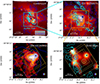 |
Fig. 1. MIRI, MUSE, and ALMA observations of NGC 1365. Upper left: Continuum map from MUSE data obtained collapsing the data in the wavelength range 5200–5800 Å. Upper right: [O III] λ5007 Å flux map from MUSE data in the ALMA FoV. Lower left: [Fe VII] λ6087 Å flux map from MUSE data in the MIRI Ch4 FoV. Lower right: [S III]18.51 μm flux map from MIRI data. Dashed orange rectangles represent the MIRI MRS channels FoV. Blue and green circles of radius of 0.7″ represent the regions from which we extracted the spectra shown in Fig. 2. Cyan and blue contours represent arbitrary levels of CO(3-2) flux from ALMA and [O III] λ5007 Å from MUSE, respectively. The star marks the position of the nucleus based on the ALMA data (see Section A.3). In the lower panels, the violet and orange circles represent the MUSE and MIRI PSF, respectively. The ALMA beam is shown as a cyan oval. |
As is shown in Fig. 2, the MIRI spectra also exhibit at least 15 bright PAH features in the wavelength range between 5–18 μm, which we will investigate in a dedicated forthcoming paper. To obtain these spectra, for the first time we combined the emission from all 12 MIRI datacubes, taking into account the different pixel sizes and ensuring a proper flux conservation among different bands by applying a scaling factor to align the flux levels between adjacent bands. A detailed description of this novel procedure is presented in the Appendix B. This algorithm, written in Python, is available for download1.
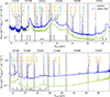 |
Fig. 2. Integrated spectra of NGC 1365 from MIRI MRS data. The blue and green curves represent the integrated spectra extracted from the 0.7″ radius apertures marked by the circles in the lower right panel of Fig. 1. These apertures sample regions dominated by the stellar disk and outflow emission, respectively. Detected emission lines are marked with vertical lines: ionized gas emission lines are labeled in yellow, H2 rotational lines in cyan, and H I recombination lines in green. We annotate the main PAH features with gray arrows. The names of each MIRI MRS sub-channel are indicated, and the gray regions represent the overlapping spectral ranges of two adjacent sub-channels. |
In Appendix C.1, we analyzed the MIRI MRS datacubes using a customized python script to enhance the S/N with spatial smoothing, subtract the local continuum around all the brightest emission lines and then fit them spaxel by spaxel. The fit emission lines are listed in Table C.1.
The MUSE IFU observations of NGC 1365 were obtained on the 12th October 2014, under program 094.B-0321(A) (PI A. Marconi) and are part of the “Measuring AGN Under MUSE” (MAGNUM) survey (Cresci et al. 2015; Venturi et al. 2017, 2018; Mingozzi et al. 2019; Marconcini et al. 2023, 2025b). We applied the same data reduction pipeline that has been extensively applied in previous works (e.g., Venturi et al. 2018; Mingozzi et al. 2019), and which has been validated and described in detail therein. To trace the cold molecular gas, we used archival ALMA 12-m Band 7 observations (program 2016.1.00296.S, PI F.Combes; Combes et al. 2019) of the CO J = 3 → 2 transition at 345.796 GHz (rest-frame). The observation description, data reduction and emission line fitting procedure of the MUSE and ALMA data can be found in Appendices A.2–C.2 and A.3–C.3, respectively.
3. Results
3.1. Multiphase gas kinematics
For the kinematic analysis, we focused on emission lines within MIRI Ch3 (0.2″/pixel in a 6.6″ × 7.7″ FoV, corresponding to 19 pc/pixel over a 620 × 730 pc2 FoV) because of the good balance between spatial resolution and field coverage. Moreover, the Ch3 emission lines are among the brightest detected in our data, allowing us to present spatially resolved results representative of the ionized and molecular emission, with sufficient S/N across the entire FoV. Although in this analysis we focus on the FoV of Ch3, which also includes a fraction of disk gas illuminated by the AGN and not part of the outflow, it would be more accurate to refer to this region as the ionization cone rather than calling it outflow. However, we will assume in the following that all the gas in the ionization cone is in outflow.
Figure 3 shows the moment maps of [Ne V] λ14 μm, [Ne II] λ13 μm, H2 0 − 0 S(1), and CO(3-2), obtained from the emission line fitting routines presented in Appendices C.1 and C.3. The [Ne V] λ14 μm seems to follow the direction of the ionized outflow; that is, the SE-NW direction (Venturi et al. 2018), as expected from species with high-IP (see Table C.1). Its velocity field is also consistent with the [O III] λ5007 Å kinematics, which is blueshifted in the SE and redshifted in the NW. In the SE (NW) cone, we estimate gas projected velocities up to −120 km s−1 (+100 km s−1). The velocity dispersion map of [Ne V] λ14 μm shows a donut-shaped structure in SE direction of the nucleus (highlighted with contours in Fig. 4), at a projected distance of ∼2.5″ (∼240 pc), with a peak of σ ∼ 170 km s−1.
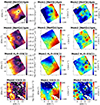 |
Fig. 3. Moment maps of ionized and molecular gas emission in NGC 1365, tracing both the rotating disk and the outflowing gas components. From top to bottom: [Ne V] λ14 μm, [Ne II] λ13 μm, H2 0 − 0 S(1), and CO(3-2) moment maps. From left to right, we show the flux, the line-of-sight velocity (LOSV), and the velocity dispersion map. The contours represent arbitrary flux levels of [Ne V] λ14 μm emission. The star marks the nucleus position. The maps size is 870 × 910 pc2. Spaxels with S/N < 5 are masked. |
The lower-IP [Ne II] λ13 μm emission line has a different morphology with respect to the highly ionized gas traced by the [Ne V] λ14 μm, suggesting that it traces a different gas component. Indeed, the [Ne II] λ13 μm morphology resembles the stellar continuum emission in the circumnuclear ring (whose ALMA contours are highlighted in Fig. 1; see also Liu et al. 2023), as we can see in Fig. 3. Moreover, the moment-0 map reveals bright clumps and lanes in the left part of the FoV that match remarkably well the features visible in Hα map of Venturi et al. (2018). This supports the interpretation that the [Ne II] λ13 μm line predominantly traces the circumnuclear ring. This includes the elongated structure ∼4″ eastward of the nucleus, which is part of the so-called “mid-east” region – associated with the Southern Arm, a stream of gas flowing in from the southeast along the bar – and is interpreted as material moving downstream within the circumnuclear ring (Liu et al. 2023). The fact that [Ne II] λ13 μm traces the disk component is also confirmed by the velocity gradient of [Ne II] λ13 μm, whose direction, along the galaxy disk major axis, and magnitude (∼120 km s−1) are consistent with those of the rotating stellar component (and Hα) observed on the same scales by Venturi et al. (2018).
The warm molecular gas component, which is traced by the H2 0-0 S(1) emission line, shares a similar morphology as that of the [Ne II] λ13 μm line (Fig. 3). The warm molecular gas flux peaks at larger distances from the nucleus and appears more diffuse, closely resembling the CO(3–2) emission. In contrast, the ionized gas traced by [Ne II] λ13 μm is concentrated in more compact regions. Since the spatial resolution at the wavelengths of the two lines is comparable, this difference in morphology reflects an intrinsic difference in the extent of the emitting regions. In addition, we observe a concentration of warm molecular gas at the position of the nucleus, which could be explained by the presence of large amounts of dust (as seen in dust continuum from MIRI by Liu et al. 2023) shielding the molecules from the AGN radiation. The kinematics follows the same rotational pattern observed in [Ne II] λ13 μm, with some deviations from a pure rotating disk. In particular, the NW side of the H2 velocity map shows lower blueshifted velocities compared to the [Ne II] λ13 μm velocity. On the opposite side, a deviation from rotation is observed in the redshifted region, which is co-spatial with an enhancement in velocity dispersion. This region, located 2″ south of the nucleus, exhibits a peak in dispersion reaching 80 km s−1 and appears as a distinct region.
The CO(3-2) moment maps shown in Fig. 3 are in agreement with the H2 0 − 0 S(1) kinematics, which is tracing the galaxy rotating disk. A similar CO velocity field was reported by Liu et al. (2023). This finding, which is consistent with the lack of any molecular outflow in the circumnuclear region (see also Combes et al. 2019), is in contrast to the CO (1-0) wind reported by Gao et al. (2021). Their outflow interpretation was based on velocity residuals from a rotating disk model on larger spatial scales, which resemble those observed in Hα and are more likely due to noncircular inflowing motions along the bar (see their Fig. 6). Notably, the cold gas traced by the CO(3-2) does not show the σ-enhanced region south of the nucleus as the H2, although both emission lines map the molecular gas. This suggests that the elevated velocity dispersion in H2 may trace noncircular motions, possibly related to local turbulence or streaming motions induced by the AGN, rather than a genuine outflow. In such an environment, the cold molecular gas traced by CO may not survive due to stronger dissociation or heating, leaving only the warm phase observable in this disturbed region.
The moment maps of the other emission lines listed in Table C.1 are shown in the online material, divided into molecular gas, recombination lines, and species with low (< 25 eV), medium (> 25 and < 54 eV), and high (> 54 eV) IP. The thresholds are based on the IPs of He I (∼25 eV) and He II (∼54 eV). Note that while some lines appear to lack emission in the nuclear region of the galaxy in the moment maps, this is because the spectra are dominated by strong continuum emission rather than a genuine absence of emission. Grouping such emission lines by IP or gas phase leads to interesting typical patterns. All the H2 lines share kinematic features similar to those of H2 0 − 0 S(1) in Fig. 3, with a rotational disk kinematics and a high-σ blob to the south of the nucleus. The low-IP lines, as well as the recombination lines, show a velocity gradient consistent with a rotating disk, with an amplitude of ∼110 km s−1, like [Ne II] λ13 μm. The high-σ region observed in H2 is not present in all the low-IP and recombination lines. From the flux maps, we observed that these species are located mainly in the mid-east region (Liu et al. 2023). The moment maps of the high-IP species are similar to those of [Ne V] λ14 μm (see Fig. 3). In particular, the donut-shaped structure is well defined in the velocity dispersion maps, although in the Ch4 the spatial resolution is lower and the shape is not well recognizable. The medium-IP lines have intermediate properties compared to the previous two groups: the velocity gradient is similar to that of the low-IP lines, but the velocity dispersion maps show a high-velocity dispersion region in correspondence of the donut shape.
3.2. Velocity channel maps
Fig. 4 presents the velocity channel maps of the [O III] λ5007 Å and [Ne V] λ14 μm emission lines, approximately spanning the velocity range from −450 km s−1 to +550 km s−1 around the same systemic velocity. Both ionic species share the same kinematic structures in each velocity bin, although [Ne V] λ14 μm appears to trace regions closer to the outflow axis, as also found by Mingozzi et al. (2019) for high-ionization gas in MAGNUM galaxies. This is consistent with the fact that both trace the outflow but are associated with different IPs (∼97 eV and ∼35 eV for [Ne V] and [O III], respectively; see Table C.1). Indeed, [Ne V] λ14 μm emission arises from more internal regions of the outflow, where the AGN radiation field is expected to be stronger. Interestingly, Fig. 3 shows that at projected velocities larger than 100 km s−1, the [Ne V] λ14 μm emission resembles the donut-shaped structure mentioned above. The bulk of the emission progressively shifts away from the nucleus with increasing channel velocity, tracing the lower arm of the donut-shaped structure. Moreover, unlike [O III] λ5007 Å, the redshifted [Ne V] λ14 μm velocity channels clearly reveal the receding NW ionization cone, which is otherwise highly obscured in the optical due to dust in the galaxy disk. Indeed, as is discussed in the following, the NW cone lies behind the disk and suffers stronger extinction than the SE cone (Venturi et al. 2017, 2018; Marconcini et al. 2025b). Thanks to the lower dust attenuation in the mid-IR, the [Ne V] λ14 μm line is an optimal tracer of this obscured outflowing component.
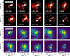 |
Fig. 4. Channel maps of ionized gas species tracing the outflow kinematics from MIRI and MUSE data. Upper panel: Channel maps of [Ne V] λ14 μm emission lines from MIRI data. Lower panel: Channel maps of [O III] λ5007 Å emission from WFM MUSE data. Contours indicate velocity dispersion levels of 97, 114, and 130 km s−1 in the [Ne V] λ14 μm emission. Velocity bins are indicated at the top of every panel in kilometers per second and are computed relative to the same systemic velocity. The star marks the position of the nucleus based on the ALMA data (see Appendix A.3). |
3.3. Resolved diagnostic diagrams for gas excitation
Diagnostic diagrams featuring mid-IR emission line ratios are widely used to investigate the nature of the gas ionizing sources (e.g., Hao et al. 2009; Weaver et al. 2010; Inami et al. 2013; Richardson et al. 2022; Martínez-Paredes et al. 2023; Feltre et al. 2023; Garofali et al. 2024; Mingozzi et al. 2025). In particular, to investigate the gas excitation in the circumnuclear region of NGC 1365, we employed mid-IR line ratios recently proposed by Feltre et al. (2023), who analyzed integrated nuclear spectra of 42 local Seyfert galaxies observed with Spitzer, including NGC 1365. To ensure consistent comparisons between line ratios, we corrected the flux maps of each emission line for differences in FoV, pixel scale, and point spread functions (PSFs). In practice, for each diagnostic diagram we adopted the FoV, pixel size, and PSF corresponding to the worst case among the lines involved, as is described below. Additionally, as is detailed in Appendix B, we applied multiplicative correction factors to account for flux discontinuities between the datacubes (see Fig. B.2).
In the upper left panel of Fig. 5, we show the contours of line ratio model predictions for AGN (Feltre et al. 2023), SF galaxies (Gutkin et al. 2016), and shocks (Alarie & Morisset 2019) for the [O IV] λ26 μm/[Ne II] λ12 μm and [Ne III] λ15 μm/[Ne II] λ12 μm line ratios. For this diagnostic diagram, we adopted the smallest FoV (6.6″ × 7.7″, i.e., Ch3), the largest pixel size (0.35″ from Ch4), and convolved all images to the worst PSF (i.e., ∼1.0″, the one at the reddest wavelength of ∼26 μm). We include all available model grids, applying only a metallicity cut of Z > 0.006 (see Feltre et al. 2023 for further details on the models). We overlay our data on model predictions, where each pixel is color-coded based on its position in the corresponding diagnostic diagram. This diagram shows that the main ionization source in the circumnuclear region of NGC 1365 can either be shocks or AGN, while no evidence for SF excitation is detected. According to Fig. 5 of Feltre et al. (2023), adding fractional contributions from SF and shock models to an AGN model will shift the points toward the bottom left in the diagram. Therefore, we classify as shock- or AGN-excited only those spaxels that fall entirely within a single predicted region. Data points located in overlapping or unclassified regions cannot be uniquely attributed to a single excitation mechanism. To better visualize the spatial distribution and morphology of these regions, we produced diagnostic maps using the same color-coding of the diagrams, as is shown in the lower panels of Fig. 5.
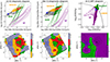 |
Fig. 5. Comparison between mid-IR and optical diagnostic diagrams. Top panels, from left to right: Diagnostic diagram of [Ne III] λ15 μm/[Ne II] λ12 μm vs. [O IV] λ14 μm/[Ne II] λ12 μm, [Ne III] λ15 μm/[Ne II] λ12 μm vs. [Ne V] λ14 μm/[Ne II] λ12 μm, and [S II] λλ6716, 6731/Hα vs. [O III] λ5007 Å/Hβ. In the mid-IR diagnostic diagrams, data points are color-coded by their proximity to the SF-, AGN-, and shocks-excitation models, based on the predictions by Feltre et al. (2023). In the [S II] BPT diagram, the solid curve defines the theoretical upper bound for pure SF (Kewley et al. 2001), while the dashed one separates Seyfert galaxies from LINERs (Kewley et al. 2006). The lower panels show spatially resolved excitation maps, where each pixel is color-coded based on its position in the corresponding diagnostic diagram. In the mid-IR diagnostic diagrams, shock-excited spaxels are in orange, AGN-excited spaxels in green, overlapping spaxels are in red, and spaxels not reproducible with any single model are in gray. In the [S II] BPT diagram, Seyfert-excited spaxels are in green, and SF-excited spaxels are in purple. Solid black contours represent arbitrary [Ne V] λ14 μm flux levels, while dashed black contours represent arbitrary levels of CO(3-2) flux from ALMA data. Circles are the regions where colored crosses in the upper panels and spectra in Fig. 2 are extracted from, integrated with a radius of 0.7″. The star marks the position of the nucleus based on the ALMA data (see Appendix A.3). Spaxels with S/N < 10 are masked. |
In the central column of Fig. 5, we show the [Ne III] λ15 μm/[Ne II] λ12 μm versus [Ne V] λ14 μm/[Ne II] λ12 μm diagnostic diagram. In this case, all lines fall within the same channel. Therefore, only the PSF convolution was required, while the FoV and pixel scale were already consistent across the maps. Similarly to the [O IV] diagram, the data points are separated into shock- and/or AGN-excited models. The [O IV] and [Ne V] excitation maps reveal similar spatial structures: an extended region dominated by AGN and combined shock/AGN excitation, aligned with the disk major axis and delimited on either side by shock-dominated zones. Notably, the eastern shock front coincides with the edge of the circumnuclear ring traced by CO and Hα (see Fig. 3 and Venturi et al. 2018), which may indicate that the outflow, emerging from the disk, interacts with the material of the circumnuclear ring, producing shocks along its path. In contrast, the centrally elongated feature may reflect direct AGN ionization within the disk.
However, Laor (1998) showed that photoionizing shocks are extremely inefficient in powering the narrow line emission in AGNs. Furthermore, as has been noted by Feltre et al. (2023), the predictions from shock models largely overlap with both AGN and star-formation grids in diagnostic diagrams. For these reasons, in Section 3.5 we consider only AGN and SF grids to model the optical and mid-IR emission lines.
Exploiting optical MUSE data, we compare the mid-IR diagnostic diagrams with the optical [S II] BPT diagram (Kewley et al. 2006, 2013) shown in the right column of Fig. 5. Moreover, we also considered the [N II] and [O I] BPT diagrams, finding similar results (see Fig. 5 in Venturi et al. 2018 and Appendix D3 in Mingozzi et al. 2019 for these diagrams at large scale). As found by Venturi et al. (2018), we notice that the circumnuclear SF ring seen in Hα and in CO (see Fig. 1) is not fully dominated by SF in the BPT diagrams. Instead, as visible from the [S II] spatial distribution, certain regions in the SE of the nucleus show signatures of AGN excitation. Venturi et al. (2018) conclude that this is likely due to the superposition along the line of sight of the AGN-ionized cone and the SF ring. The main difference between the optical BPT and the mid-IR diagnostic diagrams lies in their sensitivity to trace the true ionization source in dusty environments. In the nuclear region, the optical BPT appears to be dominated by SF due to strong dust obscuration, as is indicated by the Balmer decrement (see Appendix D and Fig. D.1). In contrast, mid-IR diagnostics can penetrate the dust screen and clearly reveal AGN ionization at the nucleus. This explains why, in the optical, AGN ionization cones are only visible on larger spatial scales, as previously shown in Venturi et al. (2018) and Mingozzi et al. (2019). Another notable difference is that the region classified as shock-dominated in the mid-IR diagrams appears to be excited by the AGN radiation according to the optical diagnostic diagram. This discrepancy likely reflects the different depths probed by optical and mid-IR emission, with mid-IR lines tracing higher ionization regions deeper into the disk, where shocks from the interaction between the outflow and the disk are expected to occur.
3.4. Electron density estimation
One of the main advantages of MIRI is the availability of mid-IR density-sensitive line ratios, such as [Ne V] λ24 μm/[Ne V] λ14 μm. These ratios are sensitive to a higher density regime with respect to the commonly used optical [S II] λ6716/[S II] λ6731 ratio, due to the different ionization energies and critical densities of the lines involved. Recent studies used IR tracers to explore the gas density in local Seyfert galaxies and found densities in the range log(ne/cm−3) = 3–5 (Hermosa Muñoz et al. 2025, 2024; Zhang et al. 2024; Ceci et al. 2025; Ramos Almeida et al. 2025).
In the top panel of Fig. 6, we show the electron density map derived from the [Ne V] λ24 μm/[Ne V] λ14 μm ratio using PyNeb (Luridiana et al. 2015), assuming an electron temperature Te = 104 K (following typical values adopted for ionized gas in AGN narrow-line regions; Osterbrock & Ferland 2006). Across the FoV, we estimate a median electron density of log(ne/cm−3) = (2.7 ± 0.5), with a peak of log(ne/cm−3) ∼ 3.5 at the nucleus. The density cannot be computed in some spaxels where the [Ne V] line ratio exceeds the lower density limit (LDL) of ∼1.2. In these spaxels, we can assume an upper limit for the density of log(ne/cm−3) ≤ 2. In the remaining regions, the morphology of the density map appears to follow the conical structure of the outflow, as traced by the [Ne V] λ14 μm emission line (see Fig. 3).
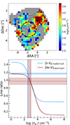 |
Fig. 6. Density map from [Ne V] and comparison with [S II]-based values. Top panel: Electron density map derived from the [Ne V] λ24 μm/[Ne V] λ14 μm line ratio. Gray pixels indicate regions where the observed ratio exceeds the theoretical low-density limit (LDL) of ∼1.2. In these spaxels, we can assume an upper limit for the density of log(ne/cm−3) ≤ 2. Black contours trace arbitrary flux levels of [Ne V] λ14 μm emission. The black circle marks the 1.5″ radius aperture used to extract integrated densities from [S II] and [Ne V]. Spaxels with S/N < 10 are masked out. Bottom panel: Theoretical [S II] and [Ne V] line ratios as a function of electron density, computed with PyNeb (Luridiana et al. 2015). Vertical dashed lines indicate the density values in the circular aperture inferred from the observed ratios (shown as horizontal dashed lines) and shaded regions represent the errors. |
Additionally, as is shown in Appendix D, we computed the electron density map from the [S II] λλ6716, 6731 doublet observed in the MUSE data (see Venturi et al. 2018 and Mingozzi et al. 2019 for the maps in the entire MUSE FoV). Both the circumnuclear ring and the outflow region are characterized by peaks in electron density, with values reaching log(ne/cm−3) ∼ 2.6–2.8. This spatial distribution is consistent with the findings of Venturi et al. (2018) and Kakkad et al. (2018), who reported enhanced electron densities in similar structures. For a quantitative comparison between the optical and mid-IR tracers, we measured the electron density from integrated spectra extracted within a 1.5″ (∼140 pc) radius aperture centered on the outflow region (see Fig. 6), using both the mid-IR and optical tracers. From the mid-IR [Ne V] line ratio, we estimate an electron density of (750 ± 440) cm−3, while from the [S II] lines we find a consistent value of (350 ± 40) cm−3. These values are illustrated in the bottom panel of Fig. 6, where we plot the theoretical [S II] and [Ne V] line ratios as functions of electron density using PyNeb (Luridiana et al. 2015), assuming an electron temperature Te = 104 K.
Based on our analysis, the gas density derived from the mid-IR diagnostics is ≈0.3 dex higher than the one derived from the optical, although consistent within the error. This difference is in agreement with the findings of Ramos Almeida et al. (2025), who reported similar, or even larger, offsets in a sample of five Type-2 quasars. Following Ramos Almeida et al. (2025), we also attribute this discrepancy to the different physical conditions probed by the two tracers: optical lines such as [S II] λλ6716, 6731 are more sensitive to diffuse, lower-density gas, while mid-IR fine-structure lines trace denser and more obscured regions, typically located closer to the AGN and less affected by dust extinction.
Our attempt to compute ne from the [Ar V] λ13 μm/[Ar V] λ8 μm ratio within the 1.5″-radius aperture interestingly yielded a ratio of ∼2.1, which is above the [Ar V] LDL value of ∼1.8 (corresponding to an upper limit on log(ne/cm−3) density similar to the [Ne V] one, ∼2). More importantly, even when integrating the [Ne V] flux across the entire MIRI FoV, we do not observe line ratios falling in the LDL, contrary to what was found by Dudik et al. (2007) using Spitzer/IRS data. This further supports the idea that their higher [Ne V] λ24 μm/[Ne V] λ14 μm ratios – and apparent detection of LDL conditions – may originate from observational limitations. In particular, the higher sensitivity of JWST/MIRI MRS compared to Spitzer/IRS may have allowed for a more effective detection of low surface brightness emission that could have remained undetected in previous studies. A direct comparison with the Dudik et al. (2007) measurements and observational setup is presented in Appendix E.
3.5. Photoionization modeling with HOMERUN
We modeled the full set of optical to mid-IR emission using state-of-the-art photoionization models. Specifically, we employed the Highly Optimized Multi-cloud Emission-line Ratios Using photo-ionizatioN (HOMERUN) modeling framework developed by Marconi et al. (2024).
3.5.1. Model grids of AGNs and SF
Given the superposition along the line of sight of the AGN-ionized cone and the circumnuclear SF ring, in the HOMERUN fit we combined two suites of models: one reproducing the emission of dust-free gas ionized by the AGN, and another accounting for the SF contribution, modeled as emission from dusty nebulae around H II regions and including both dust depletion and dust physics. Both components were assumed to have the same metallicity; however, while we adopted dust-free models for the AGN component, we included dust in the SF models and corrected gas-phase metallicities using the depletion factors listed in Table 7.8 of Hazy 1 (Cloudy v23.1). This choice was motivated by the optical extinction map (Appendix D), which shows clear dust structures associated with the SF ring, but not with the outflowing AGN-ionized gas. Furthermore, the AGN-ionized component exhibits iron coronal lines, indicating that at least part of the dust has been destroyed, releasing iron into the gas phase.
Specifically, the shape of the AGN ionizing radiation field is described by a power law with UV slope αUV = −0.5, an exponential cutoff exp(−hν/k TMax) and the X-ray component slope of αX = −1.0 linked to the UV through the αox. We have computed models with the following combinations of log(TMax/K) = 4.0, 4.5, 5.0, 5.5, 6.0, 6.5, 7.0 and αox = −1.2, −1.5, −1.8.
As is described in Marconi et al. (2024), the incident spectra for the SF model grids are stellar population models from BPASS v2.3 (Byrne et al. 2022; Stanway & Eldridge 2018) including binary stellar evolution. These models use a Kroupa (2001) initial mass function and an upper mass cutoff of 300 M⊙. We selected models with solar value for the stellar metallicity log(Zstar) = − 1.7 and ages in log(age/Myr) of 6.0, 6.4, 6.6, 7.1, 8.8.
The other model parameters are identical for the two suites of models (AGN and SF); namely, the ionization parameter log(U) (i.e., the number of ionizing photons compared to that of atoms of neutral hydrogen) ranges from −4.0 to −0.5 in step of 0.5 and the hydrogen density of the gas, log(nH/cm−3) from 0 to 7 in steps of 1. For the first iteration HOMERUN spans metallicities log(Z/Z⊙) from −1.0 to 0.4 in steps of 0.2. After this first iteration, HOMERUN performs a final refinement in steps 0.02 on predictions interpolated across the finer grid.
3.5.2. HOMERUN modeling approach
The HOMERUN models the line emission with a weighted combination of multiple CLOUDY single-cloud photoionization models (Ferland et al. 1998), iterating over different gas metallicities and incident radiation fields. The novelty of this method is that the weights assigned to the individual single-cloud models are treated as free parameters during the fitting process.
As is explained in detail in Marconi et al. (2024), the fitting process starts by selecting a grid of CLOUDY models, defined by hydrogen density (nH) and ionization parameter (U) for a fixed ionizing spectrum (Sν), gas phase oxygen abundance (AO), and elemental abundance ratios (Z). For each grid, the code searches for the best-fitting multicloud model by combining individual single-cloud templates. This is achieved by solving a non-negative least squares problem, whereby the weights of each cloud are constrained to be non-negative. The procedure is conceptually analogous to stellar population fitting methods (e.g., pPXF; Cappellari & Emsellem 2004), where a galaxy spectrum is reproduced as a linear combination of stellar templates with positive weights. No regularization is applied in the minimization, allowing for full flexibility in the weight distribution. The process is repeated across all available grids, spanning different ionizing continua, metallicities, and abundance scalings. The optimal solution is identified as the one minimizing the loss function Lmin(Sν, AO, Z), which quantifies the deviation between model predictions and observed emission-line fluxes. This loss function is effectively a reduced χ2 statistic, so values ≲1 indicate a statistically good fit.
When exploring different metallicities, elemental abundances were scaled from the solar photospheric values of Asplund et al. (2021), except for carbon and nitrogen, which were rescaled following the prescriptions of Nicholls et al. (2017). During the fit, all elemental abundances except oxygen were allowed to vary from their initial values. Scaling factors were used for the AGN and SF components. Since the AGN component was assumed to be dust-free, while the SF component includes dust, refractory elements can have different scaling factors (due to depletion), whereas non-refractory elements share the same scaling factor in both components.
3.5.3. HOMERUN fitting results
We fit the fluxes of 60 ionized and neutral atomic emission lines measured from the MIRI and MUSE spectra (32 from MIRI and 28 from MUSE, see Figs. 2 and A.1) extracted within a 1.5″ radius aperture centered on the outflow region (see Fig. 6). This aperture was chosen as the largest circular region that is fully covered by all MIRI channels, ensuring the detection of the maximum number of emission lines. The unique approach of HOMERUN enables us to reproduce at the same time 60 different emission lines in different ionization stages, with the majority of them reproduced with better than 15% accuracy. The data are best matched by a SF component with mean AV = 3.3, log(nH/cm−3) = 1.3, and log(U) = −3.3 and an AGN component with mean AV = 1.4,  /cm−3) = 2.9, and log(U) = −1.4 (see Fig. 7). Being results of ionized gas region, in the following we will consider nH = ne.
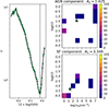 |
Fig. 7. HOMERUN model results using two component. Left panel: Variation in the loss function, ℒ, as a function of the oxygen abundance, 12 + log(O/H). In this scale, the solar metallicity is 8.69. The vertical dashed black line represents the metallicity of the model with the minimum value of ℒ. Right panels: Grids of single-cloud models in log(U) and log(nH) for the two components of the fit. The colors represent the weights of each single-cloud model, as indicated by the color bar, when ℒ reaches the minimum value. The star represents the weighted density and ionization parameter of the single-cloud models. |
We find that the SF component is more dust-attenuated than the outflow, in agreement with the extinction map obtained from the Balmer decrement (see Fig. D.1) where the higher AV values trace the circumnuclear ring and the nucleus. Interestingly, the difference in AV between SF and AGN components is in line with the median values found in MAGNUM galaxies dividing the emission in disk and outflow (Mingozzi et al. 2019). In Section 3.4, we computed the electron density from the mid-IR [Ne V] and the optical [S II] line doublet ratios within the same 1.5″ radius aperture. The density derived from [Ne V], log(ne/cm−3) ∼ 2.87, is consistent with the average value of the AGN model components, log(ne/cm−3) = 2.9. This is expected since HOMERUN attributes the entire emission of [Ne V] to the AGN (see Table F.2), as stars may not produce hard-enough radiation to account for the emission of this transition. Conversely, the [S II] lines yield a higher density of log(ne/cm−3) ∼ 2.5 within the 1.5″ radius aperture, compared to log(ne/cm−3) ∼ 1.3 from HOMERUN. This is because the average density of the SF component from HOMERUN is lower than that from the [S II] doublet and HOMERUN requires a contribution of more than 70% from the SF component to reproduce the [S II] emission (see Table F.1). This highlights the strength of our decomposition method: while classical [S II] diagnostics measure a global electron density, HOMERUN disentangles the different ionizing sources and shows that the SF component alone has a much lower density. Finally, the derived ionization parameters are log(U) = − 1.4 for the AGN component and a lower log(U) of −3.3 for the SF component, both in line with values found in H II regions (e.g., Kewley et al. 2001; Dopita et al. 2006) and AGN narrow-line regions (e.g., Groves et al. 2004). This supports the effectiveness of our decomposition in isolating distinct ionization regimes.
Figure 7 shows the results of the fit. The left panel shows the behavior of the loss function as a function of oxygen abundance. The minimum of the curve is found for the minimum loss function of ℒmin = 0.6, corresponding to 12 + log(O/H) = 8.91. The left panels represent the weights of the single-cloud models with different U and NH which were derived for the best fit, for the AGN and SF components in the upper and lower panel, respectively. Using the weights, it is possible to compute the average density and ionization parameter of the clouds, which are identified by the green star. Only a small number of single-cloud models have non-zero weights, and the AGN and SF components contribute differently across the various lines, depending on the ionization state. In particular, as is indicated in Tables F.1 and F.2, high-ionization lines (e.g., Ne V, O III) are predominantly reproduced by the AGN component, while lower-ionization lines (e.g., N II, Cl II, Ar II) are mainly explained by the SF component. Interestingly, the Hα luminosity is produced more than 70% by AGN excitation.
Using the same procedure, we fit with HOMERUN the emission lines in the spectra extracted from the regions marked in Fig. 1 (see Figs. 2 and A.1). In the outflow-dominated region (green spectrum), we find for the SF component AV = 2.8, log(nH/cm−3) = 0.9, and log(U) = −3.4, and for the AGN component AV = 1.4, log(nH/cm−3) = 3.3, and log(U) = −1.4. In the stellar disk region (blue spectrum), we find for the SF component AV = 2.9, log(nH/cm−3) = 1.4, and log(U) = −3.3, and for the AGN component AV = 1.5, log(nH/cm−3) = 5.5, and log(U) = −1.5. These values are consistent with those obtained from the spectrum extracted within a 1.5″ radius aperture (see Fig. 6). Moreover, SF emission accounts for 64% of the Hβ luminosity in the outflow region and 88% in the stellar disk region.
3.5.4. Ionized gas mass from HOMERUN
A key outcome of the HOMERUN fitting procedure is the ability to relate the luminosity of an emission line to the mass of the ionized gas associated. Since the fit is based on a physically consistent combination of AGN and SF single-cloud models, it allows us to disentangle the contributions from the different ionizing sources and connect the observed emission to intrinsic gas properties. In this way, under the assumption that the outflowing gas is fully ionized by the AGN, we avoided including the contribution from systemic or SF-related components, ensuring that the derived masses trace the outflowing gas itself. In particular, for each component, HOMERUN provides both the intrinsic (i.e., extinction-corrected) luminosities (see Tables F.1 and F.2) and the corresponding ionized gas mass. From the underlying single-cloud CLOUDY models, one obtains for each model a surface brightness in Hβ (i.e., log LHβ/area) and a gas mass surface density (i.e., log Mion/area). These model outputs define a direct proportionality between Hβ luminosity and ionized gas mass. By rescaling this relation to the total luminosity of a specific emission line (e.g., [Ne V] or [O III]) and taking into account the AGN fraction, fAGN, as determined from the HOMERUN fit, we derive a general expression:
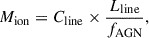 (1)
(1)
where Cline is a calibration coefficient derived from the HOMERUN AGN component models. This framework provides a robust and physically grounded method to estimate the mass of ionized outflowing gas from spatially integrated line luminosities.
After applying HOMERUN to NGC 1365 emission line fluxes, we found the following ionized gas masses:
![Mathematical equation: $$ \begin{aligned} M_{[\mathrm{O}\,\mathrm{III}]}&= 0.74\times 10^5\,M_\odot \left(\frac{L_{\rm AGN}([\mathrm{O}~\mathrm{III}])}{10^{40}\,\mathrm {erg\,s}^{-1}}\right) \end{aligned} $$](/articles/aa/full_html/2026/03/aa56352-25/aa56352-25-eq3.gif) (2)
(2)
![Mathematical equation: $$ \begin{aligned}&= 3.0 \times 10^5\,M_\odot \left(\frac{L_{\rm obs}([\mathrm{O}~\mathrm{III}])}{10^{40}\,\mathrm{erg}\,\mathrm{s}^{-1}}\right), \end{aligned} $$](/articles/aa/full_html/2026/03/aa56352-25/aa56352-25-eq4.gif) (3)
(3)
![Mathematical equation: $$ \begin{aligned} M_{[\mathrm {Ne\,V}]}&= 4.2 \times 10^5\,M_\odot \left(\frac{L_{\rm AGN}([\mathrm{Ne}~\mathrm{V}])}{10^{40}\,\text{ erg}\,\text{ s}^{-1}}\right) \end{aligned} $$](/articles/aa/full_html/2026/03/aa56352-25/aa56352-25-eq5.gif) (4)
(4)
![Mathematical equation: $$ \begin{aligned}&= 4.4 \times 10^5\,M_\odot \left(\frac{L_{\rm obs}([\mathrm{Ne}~\mathrm{V}])}{10^{40}\,\text{ erg}\,\text{ s}^{-1}}\right), \end{aligned} $$](/articles/aa/full_html/2026/03/aa56352-25/aa56352-25-eq6.gif) (5)
(5)
where LAGN([O III]) and LAGN([Ne V]) are the intrinsic line luminosities emitted by the AGN component, and Lobs([O III]) and Lobs([Ne V]) are the total observed luminosities (i.e., without the HOMERUN separation between the AGN and SF). The scaling factors applied to the observed luminosities account for both the fractional contribution of the AGN component and the effect of reddening. The scaling factors of LAGN in Equations (2) and (4) refer to extinction-corrected luminosities and can be directly compared with the standard conversion factors adopted in analytical calculations of the ionized gas masses (Equations (G.5) and (G.6), see also the discussion in the next section).
We computed an outflow mass of M[NeV] = (109 ± 2) × 103 M⊙ and M[OIII] = (88 ± 9) × 103 M⊙ within the 1.5″ radius aperture. These differences in mass, obtained with HOMERUN, reflect the discrepancy between the observed and model-predicted line ratios. Indeed, the observed ratio between [O III] λ5007 Å and [Ne V] λ14 μm fluxes is 0.81 times the model ratio (see Appendix F), which matches the ratio between the [O III] λ5007 Å- and [Ne V] λ14 μm-based outflow masses. We emphasize that the scaling relations in Equations (2)–(5) for the ionized outflow masses are not universally applicable to other AGNs. They are derived specifically from the HOMERUN multicloud modeling customized for the physical conditions and emission properties of NGC 1365. Therefore, applying these relations to other galaxies requires performing a dedicated HOMERUN fit tailored to the individual characteristics of each galaxy. In the next section, we compare the outflow mass obtained with HOMERUN modeling with that estimated following a standard and commonly used approach (e.g., Cano-Díaz et al. 2012; Carniani et al. 2015, see Appendix G and Table 1).
Properties of the ionized outflow in NGC 1365 traced by [Ne V] λ14 μm and [O III] λ5007 Å emission lines.
3.6. Outflow energetics
In the previous section, with HOMERUN we obtain an outflow mass of M[Ne V] = (109 ± 2) × 103 M⊙ and M[OIII] = (88 ± 9) × 103 M⊙ within a 1.5″ radius aperture centered on the outflow region (see Fig. 6 and Section 3.5.3). In addition, following Carniani et al. (2015), in Appendix G we present a detailed derivation of the outflow mass of [Ne V] λ14 μm and [O III] λ5007 Å. Overall, with the classic method we find in the same spatial region M[NeV] = (2.6 ± 1.0) × 103 M⊙ and M[OIII] = (20 ± 7) × 104 M⊙. The large difference between the HOMERUN and classical mass estimates (factors of ∼40 for [Ne V] and ∼2 for [O III]) clearly highlights the fundamental limitations of the standard approach. The classical method relies on several strong assumptions, such as considering that all the species are in the ionization state responsible for the observed line (e.g., O2+ for [O III], Ne4+ for [Ne V]), adopting a single average density (from [S II] in the optical and [Ne V] in the mid-IR), and correcting for attenuation using the Balmer decrement. In contrast, HOMERUN does not require assumptions about ionization levels, temperature, or metallicity, and accounts for differential reddening between the two components. The reliability of the more complex HOMERUN approach is demonstrated by the fact that classical method mass estimates differ by a factor of ∼75 between different tracers, highlighting the inherent inconsistencies of the traditional approach. Indeed, for example, the HOMERUN fitting shows that the fraction of neon in the form of Ne4+ in the best-fit models is only ∼10%, while for O2+ the fraction is significantly higher, around 60% of the total oxygen. This is certainly one of the main factors contributing to the large discrepancy between the two mass estimates. Moreover, it should be noted that [O III] and [Ne V], having different critical densities and luminosities, trace gas from slightly different physical regions within the outflowing clouds, which further contributes to the observed differences in mass estimates beyond the methodological inconsistencies of the classical approach.
We assume that the flux density within each spaxel is constant over time and that the outflow subtends a solid angle, Ω. Therefore, we computed the mass outflow rate as Ṁout = Mout vout/Δ R, i.e., the amount of ionized mass crossing a distance, ΔR, with velocity, vout. We also calculated the outflow kinetic energy as 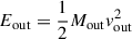 and the outflow power as
 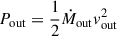 .
.
We inferred the [Ne V] λ14 μm and [O III] λ5007 Å intrinsic (i.e., de-projected) radial velocities of the outflow (vout) using the 3D multicloud MOKA3D kinematic model (Marconcini et al. 2023). This model has demonstrated exceptional power in reproducing outflow features with unprecedented detail, leveraging IFU data from a variety of instruments (Marconcini et al. 2023; Cresci et al. 2023; Perna et al. 2024; Ulivi et al. 2025; Marconcini et al. 2025a,b). To reproduce the outflow features in NGC 1365, we adopted a conical outflow morphology with maximum extension of 5 arcsec (∼470 pc) and position angle2 of 235°. The free parameters of the fit are the inclination of the cone axis with respect to the line of sight (β) and the intrinsic outflow velocity (vout). With MOKA3D we reproduce the line emission on a spaxel-by-spaxel basis, which as a consequence guarantee that the model reproduces the observed moment maps, with discrepancies between observed and modeled moment maps below 5%. We found that the best-fit parameters that reproduce the [Ne V] λ14 μm outflow features in NGC 1365 are β = 82 ± 6°, and vout = 390 ± 35 km s−1, consistent with the results in Marconcini et al. (2025b). Fig. 8 shows the 3D representation of this conical outflow. Moreover, we used MOKA3D to fit the [O III] λ5007 Å spatially resolved emission assuming the same outflow geometry as for the [Ne V] λ14 μm emission and found β = 84 ± 5°, and vout = 470 ± 40 km s−1. These results are also valid in the region where we extracted the spectrum used for the HOMERUN fitting.
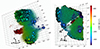 |
Fig. 8. Three-dimensional reconstruction of the MOKA3D best-fit model of the ionized outflow traced by [Ne V] λ14 μm. Gas clouds are color-coded by their LOSV. The two panels show different viewing angles: the left one provides a view into the inner cone region, while the right one corresponds to the observer’s line of sight. The XY plane represents the plane of the sky, with the Y and X axes oriented in the northern and eastern directions, respectively, while the Z axis corresponds to the line of sight. In the right panel, the dashed arrow indicate the direction of the conical outflow axis. According to the color bar, blue and red clouds are blueshifted and redshifted, respectively. Bubble size scales with the intrinsic flux of each cloud. |
So, adopting ΔR = 284 pc (∼3″, i.e., the sky-projected extension of the 1.5″ radius aperture), we obtained the results of the outflow energetics reported in Table 1. From HOMERUN, we calculated consistent mass outflow rates for [Ne V] λ14 μm and [O III] λ5007 Å, namely ![Mathematical equation: $ \dot{\mathrm{M}}_{[\rm{Ne~V}]} $](/articles/aa/full_html/2026/03/aa56352-25/aa56352-25-eq9.gif) = (1.72±0.20) × 10−1 M⊙ yr−1 and
= (1.72±0.20) × 10−1 M⊙ yr−1 and ![Mathematical equation: $ \dot{\mathrm{M}}_{[\mathrm{O~III}]} = \left(1.68 \pm 0.31\right) \times 10^{-1} $](/articles/aa/full_html/2026/03/aa56352-25/aa56352-25-eq10.gif) M⊙ yr−1, respectively. Instead, with the classic approach the [O III]-derived outflow rate is two orders of magnitude larger than that from [Ne V]. This discrepancy is primarily driven by the underestimation of the [Ne V] outflow mass in the classical approach. Specifically, the classical [Ne V] outflow mass is ∼75 times smaller than the [O III] estimate and ∼40 times smaller than the HOMERUN value, while the classical [O III] mass is only a factor of ∼2 higher than the HOMERUN mass. This asymmetric bias clearly demonstrates that the limitations of the standard method predominantly affects high-ionization tracers like [Ne V], leading to severely underestimated masses and consequently unreliable mass outflow rate calculations.
M⊙ yr−1, respectively. Instead, with the classic approach the [O III]-derived outflow rate is two orders of magnitude larger than that from [Ne V]. This discrepancy is primarily driven by the underestimation of the [Ne V] outflow mass in the classical approach. Specifically, the classical [Ne V] outflow mass is ∼75 times smaller than the [O III] estimate and ∼40 times smaller than the HOMERUN value, while the classical [O III] mass is only a factor of ∼2 higher than the HOMERUN mass. This asymmetric bias clearly demonstrates that the limitations of the standard method predominantly affects high-ionization tracers like [Ne V], leading to severely underestimated masses and consequently unreliable mass outflow rate calculations.
Our mass outflow rate estimate derived with MOKA3D + HOMERUN models is about one order of magnitude larger than the total ionized outflow rate reported by Venturi et al. (2018), which was derived from the broad Hα component in a shell-like region of the SE cone, extending from 1″ to 6″ from the nucleus. This large discrepancy clearly highlights how significantly the adopted methodology can affect the inferred outflow properties.
4. Conclusions
In this work, we have presented JWST/MIRI MRS observations of the active galaxy NGC 1365 as part of the Mid-IR Activity of Circumnuclear Line Emission (MIRACLE) program. We analyzed the spatially resolved gas properties and compared them with optical and millimeter observations from MUSE and ALMA, respectively. We traced both the ionized atomic and the warm and cold molecular gas phases in the circumnuclear region (∼0.9 × 0.9 kpc2) of the NGC 1365 galaxy, identifying more than 40 mid-IR emission lines. Our main results are the following:
-
We find that the mid-IR, optical, and millimeter emission lines consistently trace different phases of the gas with coherent internal kinematics within each phase (see Fig. 3 and Section 3.1). The cold molecular gas traced by the CO(3-2) transition shares the same ordered kinematics of the stellar galaxy disk (Venturi et al. 2018), with no evidence of outflowing material. The same conclusion holds for the warm molecular gas traced by the H2 pure-rotational transitions, with the exception of a peculiar high-σ unresolved region located southward of the nucleus.
-
The ionized gas lines can be separated in two main groups that show opposed morphologies based on their IP. The high-IP (> 54 eV) emission lines trace the bipolar outflow, showing a velocity gradient perpendicular to the disk major axis, consistent with the [O III] λ5007 Å kinematics. The velocity dispersion map highlights a donut-shaped structure associated with the approaching side of the outflow, which extends up to 2.5″ (∼240 pc). The low-IP (< 25 eV) emission line kinematics resembles the stellar galaxy disk ordered motions, similar to the H2, with clumpy flux peaks in the circumnuclear star-forming ring. Finally, medium-IP lines show intermediate properties, with a kinematics similar to low-IP species but exhibiting the donut-shaped structure typical of the high-IP lines in the velocity dispersion map.
-
[O III] λ5007 Å and [Ne V] λ14 μm velocity channel maps reveal that both outflowing species trace the same kinematic structures, with the [Ne V] λ14 μm appearing more collimated on the outflow axis, as was expected from their different IPs (Fig. 4 and Section 3.2). The [Ne V] λ14 μm emission also reveals the NW receding counterpart of the ionization cone, which is undetected in [O III] λ5007 Å due to large extinction caused by the galaxy disk at optical wavelengths.
-
The mid-IR emission-line ratios indicate a composite excitation scenario, with contributions from both AGN photoionization and shocks (Fig. 5 and Section 3.3). The AGN ionization seems to extend along the disk major axis, while in the other direction we observe shock-dominated zones, suggesting an interaction between the outflow and the disk material. Notably, by penetrating the dust in the central regions of the galaxy, these mid-IR diagnostic diagrams reveal for the first time the role of the AGN in ionizing the gas in the nuclear region, differently from the optical diagnostic diagrams that mostly reveal excitation due to SF.
-
The spatially resolved electron density map derived from the [Ne V] λ24 μm/[Ne V] λ14 μm line ratio shows a median density of (750 ± 440) cm−3 (Fig. 6), ≈0.3 dex higher than the value inferred from optical [S II] λ6716/[S II] λ6731 line ratio (see Sections 3.4 and Appendix D).
-
By exploiting the innovative photoionization modeling code HOMERUN, we derived the physical properties of the ionized outflowing gas, providing a self-consistent and physically motivated estimate of the outflow mass (Section 3.5). We obtained M[NeV] = (109 ± 2) × 103 M⊙ and M[OIII] = (88 ± 9) × 103 M⊙. These estimates differ significantly from those derived with the standard method, which are ∼40 times lower ([Ne V]) and ∼2 times higher ([O III]) than those obtained from HOMERUN. This discrepancy reflects the strong assumptions in the classical approach regarding ionization state, average density, and extinction correction.
-
We find a consistent outflow mass rate of ∼0.17 M⊙ yr−1 from [Ne V] λ14 μm and [O III] λ5007 Å (Section 3.6). Our estimate is about one order of magnitude higher than the value reported in the literature, clearly illustrating how different methods can significantly impact the inferred outflow properties. To derive the intrinsic outflow velocities, we used the 3D MOKA3D kinematic model, assuming a conical geometry. The best-fit solutions provide consistent inclination angles (β ∼ 82–84°) and outflow velocities (vout ∼ 390–470 km s−1) for both [Ne V] λ14 μm and [O III] λ5007 Å, reinforcing the reliability of our kinematic and energetic estimates.
This work highlights the critical need for self-consistent, multiline photoionization and kinematical modeling to properly capture the complex structure and energetics of AGN-driven outflows – a key step toward understanding their impact on galaxy evolution. We fully exploited the synergy between cutting-edge IFU facilities, JWST/MIRI and VLT/MUSE, to model the ionized gas phase properties across a broad ionization range (from ∼10 eV to ∼130 eV), using a total of 60 emission lines. For the first time, we combined detailed 3D kinematic modeling with MOKA^3D and photoionization fitting with HOMERUN to derive the intrinsic structure and physical conditions of the outflow in a fully self-consistent framework. This unprecedented approach enabled a coherent and physically motivated characterization of the outflow’s spatial structure, ionization stratification, and energetics. Our results show that classical methods, based on simplified assumptions and a limited set of tracers, significantly underestimate the outflow energetics – and hence the strength of AGN feedback.
Data availability
The moment maps of the other emission lines listed in Table C.1 are shown in the online material. The reduced MIRI IFU datacubes used in this work are available at the CDS via https://cdsarc.cds.unistra.fr/viz-bin/cat/J/A+A/707/A376
Acknowledgments
We are greatful to S. Charlot for kindly providing the predictions for the SF line-emission models. EB, FB, and GC acknowledge financial support from INAF under the Large Grant 2022 “The metal circle: a new sharp view of the baryon cycle up to Cosmic Dawn with the latest generation IFU facilities” and the GO grant 2024 “A JWST/MIRI MIRACLE: Mid-IR Activity of Circumnuclear Line Emission”. IL, FB, and AM acknowledge support from PRIN-MUR project “PROMETEUS” financed by the European Union – Next Generation EU, Mission 4 Component 1 CUP B53D23004750006 and C53D2300080006. EB acknowledges INAF funding through the “Ricerca Fondamentale 2024” program (mini-grant 1.05.24.07.01). AM, MG, IL and CM acknowledge INAF funding through the “Ricerca Fondamentale 2023” program (mini-grant 1.05.23.04.01). FS acknowledges financial support from the PRIN MUR 2022 2022TKPB2P – BIG-z, Ricerca Fondamentale INAF 2023 Data Analysis grant 1.05.23.03.04 “ARCHIE ARchive Cosmic HI & ISM Evolution”, Ricerca Fondamentale INAF 2024 under project 1.05.24.07.01 MINI-GRANTS RSN1 “ECHOS”, Bando Finanziamento ASI CI-UCO-DSR-2022-43, CUP C93C25004260005, project “IBISCO: feedback and obscuration in local AGN”. G.S. acknowledges the project ASI-Astrobiologia 2023 MIGLIORA (“Modeling Chemical Complexity”, F83C23000800005), the INAF-GO 2023 fundings PROTOSKA (“Exploiting ALMA data to study planet forming disks: preparing the advent of SKA”, C13C23000770005), the INAF Minigrant 2023 TRIESTE (“TRacing the chemIcal hEritage of our originS: from proTostars to planEts”; PI: G. Sabatini) and financial support under the National Recovery and Resilience Plan (NRRP), Mission 4, Component 2, Investment 1.1, Call for tender No. 104 published on 2.2.2022 by the Italian Ministry of University and Research (MUR), funded by the European Union – NextGenerationEU-Project Title 2022JC2Y93 Chemical Origins: linking the fossil composition of the Solar System with the chemistry of protoplanetary disks – CUP J53D23001600006 – Grant Assignment Decree No. 962 adopted on 30.06.2023 by the Italian Ministry of Ministry of University and Research (MUR). SC and GV acknowledge support by European Union’s HE ERC Starting Grant No. 101040227 – WINGS. JF acknowledges financial support from CONAHCyT, project number CF-2023-G100, and UNAM-DGAPA-PAPIIT IN111620 grant, Mexico. AVG acknowledges support from the Spanish grant PID2022-138560NB-I00, funded by MCIN/AEI/10.13039/501100011033/FEDER, EU. MM is thankful for support from the European Space Agency (ESA). EH gratefully acknowledges the hospitality of the IAC, where part of this work was carried out during a long research visit. This work is based on observations made with the NASA/ESA/CSA James Webb Space Telescope. The data were obtained from the Mikulski Archive for Space Telescopes at the Space Telescope Science Institute, which is operated by the Association of Universities for Research in Astronomy, Inc., under NASA contract NAS 5-03127 for JWST. The specific observations analyzed can be accessed via doi: https://doi.org/10.17909/b4w1-hk44. These observations are associated with program #6138. The authors acknowledge the team led by coPIs C. Marconcini and A. Feltre for developing their observing program with a zero-exclusive-access period. This paper makes use of the following ALMA data: ADS/JAO.ALMA#2016.1.00296.S. ALMA is a partnership of ESO (representing its member states), NSF (USA) and NINS (Japan), together with NRC (Canada), NSTC and ASIAA (Taiwan), and KASI (Republic of Korea), in cooperation with the Republic of Chile. The Joint ALMA Observatory is operated by ESO, AUI/NRAO and NAOJ.
References
- Alarie, A., & Morisset, C. 2019, Rev. Mexicana Astron. Astrofis., 55, 377 [Google Scholar]
- Alonso-Herrero, A., Sánchez-Portal, M., Ramos Almeida, C., et al. 2012, MNRAS, 425, 311 [CrossRef] [Google Scholar]
- Anand, G. S., Lee, J. C., Van Dyk, S. D., et al. 2021, MNRAS, 501, 3621 [Google Scholar]
- Argyriou, I., Wells, M., Glasse, A., et al. 2020, A&A, 641, A150 [NASA ADS] [CrossRef] [EDP Sciences] [Google Scholar]
- Argyriou, I., Glasse, A., Law, D. R., et al. 2023, A&A, 675, A111 [NASA ADS] [CrossRef] [EDP Sciences] [Google Scholar]
- Asplund, M., Grevesse, N., Sauval, A. J., & Scott, P. 2009, ARA&A, 47, 481 [NASA ADS] [CrossRef] [Google Scholar]
- Asplund, M., Amarsi, A. M., & Grevesse, N. 2021, A&A, 653, A141 [NASA ADS] [CrossRef] [EDP Sciences] [Google Scholar]
- Audibert, A., Ramos Almeida, C., García-Burillo, S., et al. 2023, A&A, 671, L12 [NASA ADS] [CrossRef] [EDP Sciences] [Google Scholar]
- Bacon, R., Accardo, M., Adjali, L., et al. 2010, SPIE Conf. Ser., 7735, 773508 [Google Scholar]
- Baldwin, J. A., Phillips, M. M., & Terlevich, R. 1981, PASP, 93, 5 [Google Scholar]
- Belli, S., Park, M., Davies, R. L., et al. 2024, Nature, 630, 54 [NASA ADS] [CrossRef] [Google Scholar]
- Boroson, T. A., & Green, R. F. 1992, ApJS, 80, 109 [Google Scholar]
- Braito, V., Reeves, J. N., Gofford, J., et al. 2014, ApJ, 795, 87 [NASA ADS] [CrossRef] [Google Scholar]
- Bureau, M., Mould, J. R., & Staveley-Smith, L. 1996, ApJ, 463, 60 [Google Scholar]
- Bushouse, H., Eisenhamer, J., Dencheva, N., et al. 2022, https://doi.org/10.5281/zenodo.6984366 [Google Scholar]
- Byrne, C. M., Stanway, E. R., Eldridge, J. J., McSwiney, L., & Townsend, O. T. 2022, MNRAS, 512, 5329 [NASA ADS] [CrossRef] [Google Scholar]
- Cano-Díaz, M., Maiolino, R., Marconi, A., et al. 2012, A&A, 537, L8 [NASA ADS] [CrossRef] [EDP Sciences] [Google Scholar]
- Cappellari, M., & Copin, Y. 2003, MNRAS, 342, 345 [Google Scholar]
- Cappellari, M., & Emsellem, E. 2004, PASP, 116, 138 [Google Scholar]
- Carniani, S., Marconi, A., Maiolino, R., et al. 2015, A&A, 580, A102 [NASA ADS] [CrossRef] [EDP Sciences] [Google Scholar]
- CASA Team (Bean, B., et al.) 2022, PASP, 134, 114501 [NASA ADS] [CrossRef] [Google Scholar]
- Ceci, M., Cresci, G., Arribas, S., et al. 2025, A&A, 695, A116 [NASA ADS] [CrossRef] [EDP Sciences] [Google Scholar]
- Cicone, C., Brusa, M., Ramos Almeida, C., et al. 2018, Nat. Astron., 2, 176 [Google Scholar]
- Combes, F. 2017, Front. Astron. Space Sci., 4, 10 [NASA ADS] [CrossRef] [Google Scholar]
- Combes, F., García-Burillo, S., Audibert, A., et al. 2019, A&A, 623, A79 [NASA ADS] [CrossRef] [EDP Sciences] [Google Scholar]
- Cresci, G., & Maiolino, R. 2018, Nat. Astron., 2, 179 [Google Scholar]
- Cresci, G., Marconi, A., Zibetti, S., et al. 2015, A&A, 582, A63 [NASA ADS] [CrossRef] [EDP Sciences] [Google Scholar]
- Cresci, G., Tozzi, G., Perna, M., et al. 2023, A&A, 672, A128 [NASA ADS] [CrossRef] [EDP Sciences] [Google Scholar]
- Davies, R., Shimizu, T., Pereira-Santaella, M., et al. 2024, A&A, 689, A263 [NASA ADS] [CrossRef] [EDP Sciences] [Google Scholar]
- de Vaucouleurs, G., de Vaucouleurs, A., Corwin, H. G., Jr., et al. 1991, Third Reference Catalogue of Bright Galaxies (Springer) [Google Scholar]
- Decleir, M., Gordon, K. D., Andrews, J. E., et al. 2022, ApJ, 930, 15 [NASA ADS] [CrossRef] [Google Scholar]
- Dopita, M. A., Fischera, J., Sutherland, R. S., et al. 2006, ApJS, 167, 177 [NASA ADS] [CrossRef] [Google Scholar]
- Dudik, R. P., Weingartner, J. C., Satyapal, S., et al. 2007, ApJ, 664, 71 [NASA ADS] [CrossRef] [Google Scholar]
- Fabian, A. C. 2012, ARA&A, 50, 455 [Google Scholar]
- Feltre, A., Gruppioni, C., Marchetti, L., et al. 2023, A&A, 675, A74 [NASA ADS] [CrossRef] [EDP Sciences] [Google Scholar]
- Ferland, G. J., Korista, K. T., Verner, D. A., et al. 1998, PASP, 110, 761 [Google Scholar]
- Feruglio, C., Maiolino, R., Piconcelli, E., et al. 2010, A&A, 518, L155 [NASA ADS] [CrossRef] [EDP Sciences] [Google Scholar]
- Fiore, F., Feruglio, C., Shankar, F., et al. 2017, A&A, 601, A143 [NASA ADS] [CrossRef] [EDP Sciences] [Google Scholar]
- Fitzpatrick, E. L., Massa, D., Gordon, K. D., Bohlin, R., & Clayton, G. C. 2019, ApJ, 886, 108 [Google Scholar]
- Fluetsch, A., Maiolino, R., Carniani, S., et al. 2019, MNRAS, 483, 4586 [NASA ADS] [Google Scholar]
- Fluetsch, A., Maiolino, R., Carniani, S., et al. 2021, MNRAS, 505, 5753 [NASA ADS] [CrossRef] [Google Scholar]
- Forbes, D. A., & Norris, R. P. 1998, MNRAS, 300, 757 [Google Scholar]
- Förster Schreiber, N. M., Übler, H., Davies, R. L., et al. 2019, ApJ, 875, 21 [Google Scholar]
- Gao, Y., Egusa, F., Liu, G., et al. 2021, ApJ, 913, 139 [NASA ADS] [CrossRef] [Google Scholar]
- García-Bernete, I., Alonso-Herrero, A., Rigopoulou, D., et al. 2024, A&A, 681, L7 [NASA ADS] [CrossRef] [EDP Sciences] [Google Scholar]
- García-Burillo, S., Combes, F., Ramos Almeida, C., et al. 2019, A&A, 632, A61 [Google Scholar]
- Garofali, K., Basu-Zych, A. R., Johnson, B. D., et al. 2024, ApJ, 960, 13 [NASA ADS] [CrossRef] [Google Scholar]
- Gordon, K. 2024, J. Open Source Softw., 9, 7023 [NASA ADS] [CrossRef] [Google Scholar]
- Gordon, K. D., Cartledge, S., & Clayton, G. C. 2009, ApJ, 705, 1320 [NASA ADS] [CrossRef] [Google Scholar]
- Gordon, K. D., Misselt, K. A., Bouwman, J., et al. 2021, ApJ, 916, 33 [NASA ADS] [CrossRef] [Google Scholar]
- Gordon, K. D., Clayton, G. C., Decleir, M., et al. 2023, ApJ, 950, 86 [CrossRef] [Google Scholar]
- Groves, B. A., Dopita, M. A., & Sutherland, R. S. 2004, ApJS, 153, 75 [NASA ADS] [CrossRef] [Google Scholar]
- Gutkin, J., Charlot, S., & Bruzual, G. 2016, MNRAS, 462, 1757 [Google Scholar]
- Hao, L., Wu, Y., Charmandaris, V., et al. 2009, ApJ, 704, 1159 [NASA ADS] [CrossRef] [Google Scholar]
- Harrison, C. M., & Ramos Almeida, C. 2024, Galaxies, 12, 17 [NASA ADS] [CrossRef] [Google Scholar]
- Harrison, C. M., Alexander, D. M., Mullaney, J. R., & Swinbank, A. M. 2014, MNRAS, 441, 3306 [Google Scholar]
- Harrison, C. M., Alexander, D. M., Mullaney, J. R., et al. 2016, MNRAS, 456, 1195 [Google Scholar]
- Hatziminaoglou, E., Zwaan, M., Andreani, P., et al. 2015, Messenger, 162, 24 [Google Scholar]
- Hermosa Muñoz, L., Alonso-Herrero, A., Pereira-Santaella, M., et al. 2024, A&A, 690, A350 [NASA ADS] [CrossRef] [EDP Sciences] [Google Scholar]
- Hermosa Muñoz, L., Alonso-Herrero, A., Labiano, A., et al. 2025, A&A, 693, A321 [NASA ADS] [CrossRef] [EDP Sciences] [Google Scholar]
- Hill, M. J., & Zakamska, N. L. 2014, MNRAS, 439, 2701 [Google Scholar]
- Inami, H., Armus, L., Charmandaris, V., et al. 2013, ApJ, 777, 156 [Google Scholar]
- Jacobs, B. A., Rizzi, L., Tully, R. B., et al. 2009, AJ, 138, 332 [NASA ADS] [CrossRef] [Google Scholar]
- Jones, J. E., & Jones, B. J. T. 1980, MNRAS, 191, 685 [CrossRef] [Google Scholar]
- Kakkad, D., Groves, B., Dopita, M., et al. 2018, A&A, 618, A6 [NASA ADS] [CrossRef] [EDP Sciences] [Google Scholar]
- Kakkad, D., Mainieri, V., Vietri, G., et al. 2020, A&A, 642, A147 [NASA ADS] [CrossRef] [EDP Sciences] [Google Scholar]
- Kewley, L. J., Dopita, M. A., Sutherland, R. S., Heisler, C. A., & Trevena, J. 2001, ApJ, 556, 121 [Google Scholar]
- Kewley, L. J., Groves, B., Kauffmann, G., & Heckman, T. 2006, MNRAS, 372, 961 [Google Scholar]
- Kewley, L. J., Maier, C., Yabe, K., et al. 2013, ApJ, 774, L10 [Google Scholar]
- Kristen, H., Jorsater, S., Lindblad, P. O., & Boksenberg, A. 1997, A&A, 328, 483 [NASA ADS] [Google Scholar]
- Kroupa, P. 2001, MNRAS, 322, 231 [NASA ADS] [CrossRef] [Google Scholar]
- Labiano, A., Argyriou, I., Álvarez-Márquez, J., et al. 2021, A&A, 656, A57 [NASA ADS] [CrossRef] [EDP Sciences] [Google Scholar]
- Laor, A. 1998, ApJ, 496, L71 [Google Scholar]
- Law, D. R., Morrison, J. E., Argyriou, I., et al. 2023, AJ, 166, 45 [NASA ADS] [CrossRef] [Google Scholar]
- Lee, J. C., Whitmore, B. C., Thilker, D. A., et al. 2022, ApJS, 258, 10 [NASA ADS] [CrossRef] [Google Scholar]
- Lee, J. C., Sandstrom, K. M., Leroy, A. K., et al. 2023, ApJ, 944, L17 [NASA ADS] [CrossRef] [Google Scholar]
- Lindblad, P. O., Hjelm, M., Hoegbom, J., et al. 1996, A&AS, 120, 403 [NASA ADS] [CrossRef] [EDP Sciences] [Google Scholar]
- Liu, D., Schinnerer, E., Cao, Y., et al. 2023, ApJ, 944, L19 [NASA ADS] [CrossRef] [Google Scholar]
- Luridiana, V., Morisset, C., & Shaw, R. A. 2015, A&A, 573, A42 [NASA ADS] [CrossRef] [EDP Sciences] [Google Scholar]
- Lutz, D., Sturm, E., Janssen, A., et al. 2020, A&A, 633, A134 [NASA ADS] [CrossRef] [EDP Sciences] [Google Scholar]
- Marasco, A., Cresci, G., Nardini, E., et al. 2020, A&A, 644, A15 [EDP Sciences] [Google Scholar]
- Marconcini, C., Marconi, A., Cresci, G., et al. 2023, A&A, 677, A58 [NASA ADS] [CrossRef] [EDP Sciences] [Google Scholar]
- Marconcini, C., Feltre, A., Lamperti, I., et al. 2025a, A&A, 701, A113 [NASA ADS] [CrossRef] [EDP Sciences] [Google Scholar]
- Marconcini, C., Marconi, A., Cresci, G., et al. 2025b, Nat. Astron., 9, 907 [Google Scholar]
- Marconi, A., Amiri, A., Feltre, A., et al. 2024, A&A, 689, A78 [NASA ADS] [CrossRef] [EDP Sciences] [Google Scholar]
- Martínez-Paredes, M., Bruzual, G., Morisset, C., et al. 2023, MNRAS, 525, 2916 [CrossRef] [Google Scholar]
- Mingozzi, M., Cresci, G., Venturi, G., et al. 2019, A&A, 622, A146 [NASA ADS] [CrossRef] [EDP Sciences] [Google Scholar]
- Mingozzi, M., Garcia del Valle-Espinosa, M., James, B. L., et al. 2025, ApJ, 985, 253 [Google Scholar]
- Morrison, J. E., Dicken, D., Argyriou, I., et al. 2023, PASP, 135, 075004 [NASA ADS] [CrossRef] [Google Scholar]
- Mulcahey, C. R., Leslie, S. K., Jackson, T. M., et al. 2022, A&A, 665, A144 [NASA ADS] [CrossRef] [EDP Sciences] [Google Scholar]
- Nicholls, D. C., Sutherland, R. S., Dopita, M. A., Kewley, L. J., & Groves, B. A. 2017, MNRAS, 466, 4403 [Google Scholar]
- Osterbrock, D. E., & Ferland, G. J. 2006, Astrophysics of Gaseous Nebulae and Active Galactic Nuclei (University Science Books) [Google Scholar]
- Patapis, P., Argyriou, I., Law, D. R., et al. 2024, A&A, 682, A53 [NASA ADS] [CrossRef] [EDP Sciences] [Google Scholar]
- Perna, M., Arribas, S., Lamperti, I., et al. 2024, A&A, 690, A171 [NASA ADS] [CrossRef] [EDP Sciences] [Google Scholar]
- Perrin, M. D., Sivaramakrishnan, A., Lajoie, C.-P., et al. 2014, SPIE Conf. Ser., 9143, 91433X [NASA ADS] [Google Scholar]
- Ramos Almeida, C., Bischetti, M., García-Burillo, S., et al. 2022, A&A, 658, A155 [NASA ADS] [CrossRef] [EDP Sciences] [Google Scholar]
- Ramos Almeida, C., García-Bernete, I., Pereira-Santaella, M., et al. 2025, A&A, 698, A194 [NASA ADS] [CrossRef] [EDP Sciences] [Google Scholar]
- Richardson, C. T., Simpson, C., Polimera, M. S., et al. 2022, ApJ, 927, 165 [NASA ADS] [CrossRef] [Google Scholar]
- Richings, A. J., & Faucher-Giguère, C.-A. 2018a, MNRAS, 478, 3100 [NASA ADS] [CrossRef] [Google Scholar]
- Richings, A. J., & Faucher-Giguère, C.-A. 2018b, MNRAS, 474, 3673 [Google Scholar]
- Rieke, G. H., Wright, G. S., Böker, T., et al. 2015, PASP, 127, 584 [NASA ADS] [CrossRef] [Google Scholar]
- Riffel, R. A., Zakamska, N. L., & Riffel, R. 2020, MNRAS, 491, 1518 [NASA ADS] [CrossRef] [Google Scholar]
- Risaliti, G., Bianchi, S., Matt, G., et al. 2005, ApJ, 630, L129 [NASA ADS] [CrossRef] [Google Scholar]
- Sakamoto, K., Ho, P. T. P., Mao, R.-Q., Matsushita, S., & Peck, A. B. 2007, ApJ, 654, 782 [Google Scholar]
- Sanchez, R. Z. 2009, Ph.D. Thesis, Rutgers University, New Jersey [Google Scholar]
- Sandqvist, A., Joersaeter, S., & Lindblad, P. O. 1995, A&A, 295, 585 [NASA ADS] [Google Scholar]
- Schinnerer, E., Emsellem, E., Henshaw, J. D., et al. 2023, ApJ, 944, L15 [NASA ADS] [CrossRef] [Google Scholar]
- Sharp, R. G., & Bland-Hawthorn, J. 2010, ApJ, 711, 818 [Google Scholar]
- Speranza, G., Ramos Almeida, C., Acosta-Pulido, J. A., et al. 2024, A&A, 681, A63 [NASA ADS] [CrossRef] [EDP Sciences] [Google Scholar]
- Stanway, E. R., & Eldridge, J. J. 2018, MNRAS, 479, 75 [NASA ADS] [CrossRef] [Google Scholar]
- Stevens, I. R., Forbes, D. A., & Norris, R. P. 1999, MNRAS, 306, 479 [Google Scholar]
- Teuben, P. J., Sanders, R. H., Atherton, P. D., & van Albada, G. D. 1986, MNRAS, 221, 1 [CrossRef] [Google Scholar]
- Tozzi, G., Cresci, G., Marasco, A., et al. 2021, A&A, 648, A99 [NASA ADS] [CrossRef] [EDP Sciences] [Google Scholar]
- Ulivi, L., Perna, M., Lamperti, I., et al. 2025, A&A, 693, A36 [NASA ADS] [CrossRef] [EDP Sciences] [Google Scholar]
- Vazdekis, A., Koleva, M., Ricciardelli, E., Röck, B., & Falcón-Barroso, J. 2016, MNRAS, 463, 3409 [Google Scholar]
- Veilleux, S., & Osterbrock, D. E. 1987, ApJS, 63, 295 [Google Scholar]
- Veilleux, S., Cecil, G., & Bland-Hawthorn, J. 2005, ARA&A, 43, 769 [NASA ADS] [CrossRef] [Google Scholar]
- Venturi, G., Marconi, A., Mingozzi, M., et al. 2017, Front. Astron. Space Sci., 4, 46 [Google Scholar]
- Venturi, G., Nardini, E., Marconi, A., et al. 2018, A&A, 619, A74 [NASA ADS] [CrossRef] [EDP Sciences] [Google Scholar]
- Venturi, G., Cresci, G., Marconi, A., et al. 2021, A&A, 648, A17 [NASA ADS] [CrossRef] [EDP Sciences] [Google Scholar]
- Venturi, G., Treister, E., Finlez, C., et al. 2023, A&A, 678, A127 [NASA ADS] [CrossRef] [EDP Sciences] [Google Scholar]
- Véron-Cetty, M. P., & Véron, P. 2006, A&A, 455, 773 [Google Scholar]
- Weaver, K. A., Meléndez, M., Mushotzky, R. F., et al. 2010, ApJ, 716, 1151 [NASA ADS] [CrossRef] [Google Scholar]
- Woo, J.-H., Bae, H.-J., Son, D., & Karouzos, M. 2016, ApJ, 817, 108 [Google Scholar]
- Wootten, A., & Thompson, A. R. 2009, IEEE Proc., 97, 1463 [NASA ADS] [CrossRef] [Google Scholar]
- Wright, G. S., Wright, D., Goodson, G. B., et al. 2015, PASP, 127, 595 [NASA ADS] [CrossRef] [Google Scholar]
- Wright, G. S., Rieke, G. H., Glasse, A., et al. 2023, PASP, 135, 048003 [NASA ADS] [CrossRef] [Google Scholar]
- Zhang, L., Packham, C., Hicks, E. K. S., et al. 2024, ApJ, 974, 195 [NASA ADS] [CrossRef] [Google Scholar]
- Zubovas, K., & Bourne, M. A. 2017, MNRAS, 468, 4956 [NASA ADS] [CrossRef] [Google Scholar]
The position angle is measured clockwise from north.
Appendix A: Observations and data reduction
In this appendix, we present the observations and data reduction for MIRI MRS, MUSE, and ALMA data.
A.1. JWST/MIRI
We refer to Marconcini et al. (2025a) for a detailed description of the different steps performed during the data reduction and briefly summarize them here. We downloaded the uncalibrated science and background observations through the Barbara A. Mikulski Archive for Space Telescopes (MAST) portal3. The data reduction process was performed using the JWST Science Calibration Pipeline (Bushouse et al. 2022) version 1.16.0 with JWST Calibration Reference Data System context file 1298. We applied all three stages of the pipeline processing, which include CALWEBB_DETECTOR1, CALWEBB_SPEC2, and CALWEBB_SPEC3 (see Argyriou et al. 2020, 2023; Morrison et al. 2023; Patapis et al. 2024). For NGC 1365, we subtracted the background emission from the 2D science images using a background frame generated from our dedicated background observations. Moreover, we performed two residual fringe corrections, both in stage 2 and 3. Additionally, to improve the final datacubes, we adopted the Exponential Modified-Shepard Method (EMSM) weighting function, which has proven to be more efficient in reducing the drizzling effect (Law et al. 2023).
Finally, we applied an astrometric correction to all the datacubes with different ΔRA and ΔDec for each band, using the ALMA astrometry as reference (details in Appendix B).
A.2. MUSE Wide Field Mode
The data were retrieved from the ESO archive4 and were already processed automatically using the standard MUSE pipeline (v1.6), with an average PSF FWHM of 0.8″. The final datacube covers a FoV of 64″× 63.4″, with a pixel size of 0.2″pixel−1. The MUSE FoV covers approximately the central 5.3 × 5.3 kpc2 of NGC 1365. MUSE resolving power in Wide Field Mode (WFM) varies from R∼ 1770 at 4800 Åto 3590 at 9300 Å. Finally, we apply a relative astrometric correction, registering the position of the continuum peak, measured in the line-free 7660-8000 Åwavelength range, to the nucleus position from the ALMA data (see Appendix A.3), as done for JWST/MIRI data (see Appendix A.1). The applied corrections were ΔRA and ΔDec shifts of (-0.78″, +0.22″).
The MUSE integrated spectra of NGC 1365 extracted from the 0.7″radius regions shown in the lower left panel of Fig. 1 are reported in Fig. A.1. The green (blue) spectrum is extracted from a region where the outflow (stellar disk) emission is predominant. We detect approximately 30 emission lines (see Table F.1) tracing different gas phases, including recombination lines, atomic lines, and lines from ionized gas.
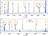 |
Fig. A.1. Integrated spectra of NGC 1365 from MUSE data. The blue and green curves represent the integrated spectra extracted with a 0.7″radius aperture from regions dominated by the stellar disk and outflow emission, respectively (see Fig. 1, lower right panel). Detected emission lines are marked with vertical lines: ionized gas emission lines in yellow, atomic lines in violet, and H I recombination lines in green. An asterisk indicates species corresponding to blends of two or three emission lines. |
A.3. ALMA
The data include observations with two different configurations with angular resolutions in FWHM of ∼0.30″and ∼0.07″, respectively. In this work, we use the observations with resolution ∼0.30″corresponding to 30 pc, which better match the MIRI MRS spatial resolution and provide a maximum recoverable scale of 2.9″. We retrieved the calibrated measurement sets using the dedicated service provided by the European ALMA Regional Center (Hatziminaoglou et al. 2015). Imaging was performed using the Common Astronomy Software Applications (CASA) v6.1.1 (CASA Team 2022). For the CO(3–2) spectral window (342.99 − 344.86 GHz), we subtracted a constant continuum level estimated from the emission line-free channels in the uv plane. The data were cleaned using the tclean task in CASA, with briggs weighting scheme with a robust parameter of 0.5, which resulted in a beam with a FWHM of 0.35″× 0.31″(beam PA = -71°), corresponding to ∼37 pc in physical scale. The final datacube has a spectral channel width of ∼8 km s−1, a pixel size of 0.05″, a FoV of 25″in diameter, and a root mean square of 1.5 mJy beam−1 per channel.
Finally, we fit the central 2″ × 2″ of the CO(3-2) flux map (see Appendix C.3) with a Gaussian profile to determine the coordinates of the nucleus, taking advantage of the high astrometric accuracy provided by ALMA. We find the nuclear position to be RA = 03h33m36.37s and Dec = -36d08m25.37s, in good agreement with the values reported by Liu et al. (2023). These coordinates are adopted throughout the rest of the paper and used to register the astrometry of MIRI and MUSE observations (see Appendices A.1 and A.2, respectively).
Appendix B: MIRI datacubes corrections
For the astrometric registration of the 12 datacubes, we applied separate corrections for each band (SHORT, MEDIUM, and LONG), as each observing setup corresponds to a different grating configuration of the MRS. As is discussed in Appendix A.1, the observations are centered on the SE outflow cone rather than the AGN. This positioning causes the source to fall near the edge, or even slightly outside, of the FoV in the Ch1 datacubes (see Fig. 1). To ensure accurate alignment across the dataset, we computed the astrometric corrections using Ch3, where the source is well within the FoV and the spatial resolution remains high, providing a reliable reference frame for registration. We collapsed the datacubes along the spectral dimension and fit the PSFs with a 2D Gaussian model. Then, we aligned the datacubes to match the PSF peaks with the AGN coordinates provided ALMA data (see Appendix A.3). The applied corrections were ΔRA and ΔDec shifts of (+0.0086″, -0.2655″), (+0.0256″, -0.2713″), and (-0.0300″, -0.299″) for the SHORT, MEDIUM, and LONG channels, respectively.
To compare flux maps of emission lines from different channels it is crucial to account for the different pixel size (see Appendix A.1). To address this, we rebinned each channel to match the pixel size of Ch4, which has the worst resolution (0.35″). We used the reproject exact function to ensure flux conservation during the resampling process. In Fig. B.1 we show the collapsed datacubes before and after the spatial rebinning. The relative flux conservation error is below the 1%, so negligible respect the original flux.
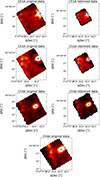 |
Fig. B.1. Examples of the rebinning procedure for datacubes in the A (SHORT) band. The first three rows compare the original collapsed data with native pixel size and FoV (left) to the rebinned data matched to the wider FoV of Ch4 (right). The bottom row shows the original Ch4 data. The star marks the nucleus position. |
MIRI data are known to exhibit flux discontinuities between different sub-channels. This effect could be amplified after the rebinning for the different pixel size of data. Therefore, it is essential to apply a scaling factor to the fluxes when constructing a single spectrum, in addition to account for differences in spectral sampling. To address this, we implemented a stitching procedure between each pair of datacubes by rescaling the flux of the bluer datacube to match the median flux value of the overlapping spectral channels of the redder datacube. We chose to rescale to the reddest datacube (Ch4 LONG) as it has the largest FoV, ensuring consistent scaling in every spaxel. This process yielded a scaling factor matrix for each pair of datacubes, which was then applied to correct all fluxes derived from our data. In Fig. B.2 an example of the total spectrum before and after the stitching procedure.
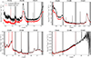 |
Fig. B.2. Comparison per channel between the original data in red and the stitched data in black. gray regions indicate overlapping spectral channels. |
As shown in Law et al. (2023), the average FWHM of the MIRI/MRS PSF varies across the four channels spanning the range FWHM = 0.4″, 0.5″, 0.6″, and 0.9″, in Ch1, Ch2, Ch3, and Ch4, respectively. This variation must be taken into account when computing ratios between emission lines at different wavelengths. To ensure consistent spatial resolution, we firstly downloaded the MIRI MRS PSF model cube using the WebbPSF tool v.1.4.0 (Perrin et al. 2014), which provide a model cube spatially oversampled of a factor of 4 with respect to the observations (i.e., 0.05 ″/pixel for Ch3). Then we deconvolved each flux map with the PSF corresponding to the wavelength of the emission line, and convolved it with the PSF at the reddest wavelength among the lines involved in the ratios, using the PSF model cubes from WebbPSF. The deconvolution procedure is composed by a wavelength-dependent alignment, rotation and flux normalization between the PSFs and our flux maps, following a similar methodology of Marconcini et al. (2025a).
Appendix C: Data analysis
In this appendix, we describe the general methodology employed for the emission line analysis of data from MUSE, ALMA, and MIRI MRS. In particular, we analyzed the MUSE and MIRI data to subtract the continuum and fit the emission lines in the optical and the mid-IR band, using a multi-Gaussian fitting procedure.
C.1. JWST/MIRI MRS emission line fitting
This appendix provides further details on the customized python routine we employed to analyze the MIRI MRS datacubes. We followed a three-step procedure: first, we applied spatial smoothing to enhance the S/N; second, we subtracted the local continuum around the brightest emission lines; finally, we performed spaxel-by-spaxel Gaussian fitting of the residual emission. First, we applied a Gaussian spatial smoothing with a kernel size of 1 pixel to every spatial plane of the datacube. This step improves the S/N of faint extended features, at the cost of a moderate degradation in spatial resolution. Specifically, the effective PSF is broadened by approximately 40% across all wavelengths, due to the fact that the pixel size is comparable to or slightly smaller than the intrinsic PSF σ at each wavelength. Nevertheless, the resulting resolution remains sufficient for our spatially resolved analysis, as it still allows us to distinguish the relevant morphological and kinematic structures in the data.
We then performed the emission line fitting spaxel-by-spaxel, fitting each line in Table C.1 independently. Prior to this, we modeled and fit the local continuum selecting wavelength windows on either side of the line, adjusting the range based on the FWHM of each emission line and carefully avoiding other spectral absorption or emission features. Given the short spectral window of ∼0.1 #x03BC;m we considered, within which the continuum is featureless, we fit the continuum with a straight line. Each emission line is modeled with both a single and a double Gaussian component, and then we applied a Kolmogorov-Smirnov (KS) test on the residuals to choose the optimal number of Gaussian components in each spaxel, adopting a threshold p-value of 0.7 (see Marasco et al. 2020; Tozzi et al. 2021; CeciSPSUNDSCR2025 for details).
List of the fit emission lines in the MIRI spectra
In the mid-IR, dust attenuation is much lower than at optical wavelengths, but it does vary with wavelength and affect emission lines differently, potentially impacting specific line ratios. Unfortunately, in our data the S/N of the Pfα and Huα (i.e., H I (6-5) at 7.46 #x03BC;m and H I (7-6) at 12.37 #x03BC;m, respectively) is too low to derive a reliable extinction map directly from the mid-IR spectra. To test the potential impact of dust attenuation, we applied an extinction correction to the mid-IR emission lines using the G23 (Gordon et al. 2009, 2021, 2023; Fitzpatrick et al. 2019; Decleir et al. 2022) attenuation curve, from the dust_extinction package5 (Gordon 2024), and adopting the maximum AV value (∼3) derived from our best-fit photoionization model (see Section 3.5.3). However, we find that the resulting variations in the mid-IR line ratios are within the errors, including those involving emission lines at distant wavelengths (e.g., [Ne V]λ24#x03BC;m/[Ne V]λ14#x03BC;m, see Section 3.4).
C.2. MUSE WFM emission line fitting
MUSE data were analyzed as already described in previous works of the MAGNUM program (Venturi et al. 2018; Mingozzi et al. 2019). Briefly, after a preliminary Voronoi tessellation (Cappellari & Copin 2003) to achieve an average S/N per wavelength channel of at least 70 on the continuum, we applied the penalized PiXel-Fitting (pPXF, Cappellari & Emsellem 2004) code to measure the optical emission lines listed in Table F.1. Using the penalized PiXel-Fitting (pPXF, Cappellari & Emsellem 2004) code, we fit simultaneously the continuum and gas emission in the wavelength range 4800-9200 Å, convolving a linear combination of stellar templates (E-MILES; for details see Vazdekis et al. 2016) with a Gaussian velocity distribution. Each emission line was fit twice, using one and two Gaussian components, and the KS test was applied spaxel-by-spaxel to determine the minimum number of components required to adequately reproduce the line profiles (see Appendix C.1). Given that NGC 1365 hosts a Seyfert 1.8 nucleus, we included an additional spectral component when fitting the bins within a radius of 10 spaxels from the nuclear position to account for the spatially unresolved broad-line region (BLR). The BLR model consists of two independent components: a broad (σ > 1000 km s−1) Gaussian component for the broad Balmer lines (i.e., Hα and Hβ) and a template of broad [Fe II] emission features by Boroson & Green (1992). The nuclear model spectrum was obtained by fitting the integrated spectrum of the central spaxels and, in the subsequent spaxel-by-spaxel fitting, it was kept fixed in shape and velocity while being allowed to scale in flux. We then subtracted the stellar and nuclear emission from the original unbinned data cube by rescaling the fit continuum - assumed constant within each Voronoi bin - to match the observed continuum flux in each spaxel, before performing the subtraction.
We obtained continuum-subtracted datacubes containing the gas emission lines only. Then, we repeated the fitting procedure applied for MIRI JWST data (see previous section). In this case, we used up to three Gaussian components to reproduce the complex line profiles and adopted a p-value of 0.9.
Finally, we corrected the optical emission-line fluxes for dust attenuation using the Balmer decrement (i.e., Hα/Hβ), assuming a case-B hydrogen recombination value of 2.86 for this ratio (for an electron temperature and density of Te = 104 K and ne = 102 cm−3, respectively; Osterbrock & Ferland 2006) and adopting the G23 attenuation law. The results, presented in Appendix D, are consistent with previous estimates by Venturi et al. (2018) and Mingozzi et al. (2019). As shown in Fig. D.1, the dust attenuation peaks at AV = 3.7 in the circumnuclear ring, where young stellar clusters are embedded (Liu et al. 2023; Schinnerer et al. 2023). High attenuation values are also found at the nuclear position, while we do not find any correlation of AV with the outflow morphology, indicative of its low dust content.
C.3. ALMA emission line fitting
We use the CO(3-2) ALMA observations to derive the kinematics of the cold molecular gas. The continuum was subtracted in the uv-plane during the data reduction (see Appendix A.3). We fit the CO(3-2) line profile in each spaxel using a single Gaussian profile, which is sufficient to reproduce the symmetric line profile. The resulting moment maps of the cold molecular gas are reported in the bottom panels of Fig. 3.
Appendix D: Extinction and electron density from MUSE
In this appendix, we present the spatially resolved maps of visual extinction and electron density in the circumnuclear region of NGC 1365, derived from the MUSE data and zoomed-in FoV matching the MIRI one. In the top panel of Fig. D.1, we show the visual extinction computed from the Balmer decrement (Hα/Hβ), adopting the G23 extinction law. High visual extinction values of AV∼ 3.7 mag are found at the nuclear position and in the SE part of the FoV, corresponding to the circumnuclear ring, as also observed by Venturi et al. (2018) and Mingozzi et al. (2019).
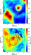 |
Fig. D.1. Spatially resolved maps of visual extinction and electron density in the circumnuclear region of NGC 1365 obtained from the MUSE data, zoomed in the MIRI FoV. Top panel: visual extinction computed from the Balmer decrement. Bottom panel: ionized gas electron density obtained from the [S II]λ6716/[S II]λ6731 line ratio. Contours represent arbitrary flux levels of [Ne V]λ14#x03BC;m. The black circle marks the 1.5″radius aperture used to extract integrated fluxes for the HOMERUN code (see Section 3.5). The star indicates the nucleus position. |
Moreover, the bottom panel of Fig. D.1 shows the electron density of the ionized gas, estimated from the total intensity of all the Gaussian components of the [S II]λλ6716, 6731 doublet. In particular, we use the [S II]λ6716/[S II]λ6731 diagnostic line ratio (Osterbrock & Ferland 2006), computed over the same FoV of the Ch4. We assume a typical value for the temperature of ionized gas of Te = 104 K and obtain the density map reported in Fig. D.1. We observe that the higher values of ne are following the outflow morphology, as traced by [Ne V]λ14#x03BC;m contours flux. In the main text, we use as average density the median value and the standard deviation of ne = (230 ± 120) cm−3 measured across the reported FoV.
Appendix E: Density comparison with IRS observations
In this appendix, we compare our spatially resolved JWST/MIRI density measurements with those obtained from integrated spectra by Dudik et al. (2007). Dudik et al. (2007) used the Infrared Spectrograph (IRS) on board Spitzer to compute the [Ne V] ratio in a sample of local AGNs. They found that Type 2 AGNs show higher line ratios with respect to Type 1, with all Type 2 sources lying above the theoretical LDL threshold, implying log(ne/cm−3) ≤ 2. In particular, for NGC 1365 they computed a [Ne V]λ24#x03BC;m/[Ne V]λ14#x03BC;m ratio of 2.4±0.6, which is larger than our estimation of 1.0±0.2 obtained as the ratio between the two integrated fluxes in the MIRI FoV. They argued that the [Ne V] emitting region likely originates inside the nuclear torus and that differential IR extinction due to dust in the obscuring torus may be responsible for the ratio above the LDL. Exploiting the spatially resolved [Ne V] emission in our data and the density values in the nuclear region, we can rule out this interpretation. However, given the presence of some LDL regions in Fig. 6, it is possible that their finding is the result of spatial integration over a wide slit, and thus including such regions in the measurement. A more plausible reason is an observational effect. Indeed, in Dudik et al. (2007) the [Ne V] fluxes were obtained using the short-wavelength, high-resolution (SH; 4.7″×11.3″, λ = 9.9-19.6 #x03BC;m) and long-wavelength, high-resolution (LH; 11.1″×22.3″, λ = 18.7-37.2 #x03BC;m) modules of IRS. As it is clear from the moment maps of the high-IP species in the online material, the extension of [Ne V] emission is detected up to 8″from the nucleus. This means that the SH module surely lost part of the [Ne V]λ14#x03BC;m flux, leading to an artificially enhancement of the [Ne V]λ24#x03BC;m/[Ne V]λ14#x03BC;m line ratio.
Appendix F: HOMERUN emission line fluxes
In this appendix we report the full list of emission lines included in the HOMERUN fit, as shown in Tables F.1 and F.2, and discussed in Section 3.5.3.
Optical emission lines fit by the HOMERUN code
Mid-IR emission lines fit by the HOMERUN code
Appendix G: Ionized gas mass estimate
In this appendix we present an analytical mass estimation for the [Ne V]λ14#x03BC;m and the [O III]λ5007 Å emission lines, in order to compute the gas masses in the 1.5″radius aperture (shown as a dashed circle in Fig. D.1) and compare them with the HOMERUN estimations in Section 3.5.4.
Following Carniani et al. (2015), we start from the luminosity of the [Ne V]λ14#x03BC;m line:
![Mathematical equation: $$ \begin{aligned} L_\text{[Ne} \text{ V]} = \int _{V} f \, n_e\, n\bigr (Ne^{4+}\bigr )\, \gamma _\text{[Ne} \text{ V]}({n_e, T_e}) dV \end{aligned} $$](/articles/aa/full_html/2026/03/aa56352-25/aa56352-25-eq11.gif) (G.1)
(G.1)
with f the filling factor, V the volume occupied by the outflowing ionized gas, ne the electron density, n(Ne4+) the density of Ne4+ ions, and γ[Ne V](ne,Te) the line emissivity. n(Ne4+) can be written as
![Mathematical equation: $$ \begin{aligned} n\left(Ne^{4+}\right)\ = \left[ \frac{ n\bigr (Ne^{4+}\bigr )}{n\left(Ne\right)} \right] \left[ \frac{ n\left(Ne\right)}{n\left(H\right)} \right] \left[ \frac{ n\left(H\right)}{n_e} \right] n_e. \end{aligned} $$](/articles/aa/full_html/2026/03/aa56352-25/aa56352-25-eq12.gif)
We assume n(Ne4+) ≈ n(Ne), ne ≈ 1.2 n(H) (i.e., a 10% number density of He atoms with respect to H atoms), and a solar abundance of [Ne/H] ∼ 7.93 (Asplund et al. 2009), to obtain n(Ne4+)∼7.09 × 10⁻⁵ ne. Assuming a typical temperature (Te ≃ 104K), from the [Ne V]λ24#x03BC;m/[Ne V]λ14#x03BC;m line ratio we find an electron density of ne = (750±440) cm−3 in the 1.5" radius aperture and estimate a line emissivity of γ[Ne V] = 1.93 × 10⁻²⁰ erg s−1 cm3 making use of PyNeb (Luridiana et al. 2015). Finally, Eq. G.1 can be rewritten as
![Mathematical equation: $$ \begin{aligned} L_\text{[Ne} \text{ V]} = 7.09 \times 10^{-5} f \, n_e^2 \, \gamma _\text{[Ne} \text{ V]} \, V, \end{aligned} $$](/articles/aa/full_html/2026/03/aa56352-25/aa56352-25-eq13.gif) (G.2)
(G.2)
assuming a constant electron density in the outflow volume. The gas mass can be expressed as
 (G.3)
(G.3)
where the average molecular weight is  = 1.27 mp, if there is a 10% fraction of He atoms, and we have taken into account that
![Mathematical equation: $$ \begin{aligned} \bar{m}\, n(H) = \bar{m} \left[ \frac{n(H)}{n_e} \right] \, n_e = 1.27 \, m_p \, (1.2)^{-1} \, n_e \approx m_p \, n_e; \end{aligned} $$](/articles/aa/full_html/2026/03/aa56352-25/aa56352-25-eq16.gif) (G.4)
(G.4)
therefore, M ≈ f mp ne V. Combining this latter with Equation G.2, we finally get
![Mathematical equation: $$ \begin{aligned} M_\text{[Ne} \text{ V]} = 3.07 \, M_\odot \left( \frac{L_\text{[Ne} \text{ V]}}{10^{36} \, \text{ erg} \, \text{ s}^{-1}} \right) \left( \frac{n_e}{200 \, \text{ cm}^{-3}} \right)^{-1}. \end{aligned} $$](/articles/aa/full_html/2026/03/aa56352-25/aa56352-25-eq17.gif) (G.5)
(G.5)
Similarly, we computed the [O III]λ5007 Å outflow mass. Using a solar abundance of [O/H] ∼ 8.69 (Asplund et al. 2009) and ne = (500 ± 270) cm−3 (from the [S II]λλ6716, 6731 ratio in the same aperture) - that leads to γ[O III] = 3.53 × 10⁻²¹ erg s−1 cm3 - we have
![Mathematical equation: $$ \begin{aligned} M_\text{[O} \text{ III]} = 2.92 \, M_\odot \left( \frac{L_\text{[O} \text{ III]}}{10^{36} \, \text{ erg} \, \text{ s}^{-1}} \right) \left( \frac{n_e}{200 \, \text{ cm}^{-3}} \right)^{-1}. \end{aligned} $$](/articles/aa/full_html/2026/03/aa56352-25/aa56352-25-eq18.gif) (G.6)
(G.6)
We corrected both the [Ne V]λ14#x03BC;m and the [O III]λ5007 Å luminosity for dust attenuation using the Balmer decrement from the Hα/Hβ ratio, employing the G23 attenuation law and an intrinsic ratio Hα/Hβ = 2.86 (for Te = 104 K, Osterbrock & Ferland 2006). Assuming the two different densities for the optical and mid-IR species previously computed, we obtain an outflow mass of M[NeV] = (2.6 ± 1.0) × 103 M⊙ and M[OIII] = (20 ± 7) × 104 M⊙.
All Tables
Properties of the ionized outflow in NGC 1365 traced by [Ne V] λ14 μm and [O III] λ5007 Å emission lines.
All Figures
|
Fig. 1. MIRI, MUSE, and ALMA observations of NGC 1365. Upper left: Continuum map from MUSE data obtained collapsing the data in the wavelength range 5200–5800 Å. Upper right: [O III] λ5007 Å flux map from MUSE data in the ALMA FoV. Lower left: [Fe VII] λ6087 Å flux map from MUSE data in the MIRI Ch4 FoV. Lower right: [S III]18.51 μm flux map from MIRI data. Dashed orange rectangles represent the MIRI MRS channels FoV. Blue and green circles of radius of 0.7″ represent the regions from which we extracted the spectra shown in Fig. 2. Cyan and blue contours represent arbitrary levels of CO(3-2) flux from ALMA and [O III] λ5007 Å from MUSE, respectively. The star marks the position of the nucleus based on the ALMA data (see Section A.3). In the lower panels, the violet and orange circles represent the MUSE and MIRI PSF, respectively. The ALMA beam is shown as a cyan oval. |
| In the text | |
|
Fig. 2. Integrated spectra of NGC 1365 from MIRI MRS data. The blue and green curves represent the integrated spectra extracted from the 0.7″ radius apertures marked by the circles in the lower right panel of Fig. 1. These apertures sample regions dominated by the stellar disk and outflow emission, respectively. Detected emission lines are marked with vertical lines: ionized gas emission lines are labeled in yellow, H2 rotational lines in cyan, and H I recombination lines in green. We annotate the main PAH features with gray arrows. The names of each MIRI MRS sub-channel are indicated, and the gray regions represent the overlapping spectral ranges of two adjacent sub-channels. |
| In the text | |
|
Fig. 3. Moment maps of ionized and molecular gas emission in NGC 1365, tracing both the rotating disk and the outflowing gas components. From top to bottom: [Ne V] λ14 μm, [Ne II] λ13 μm, H2 0 − 0 S(1), and CO(3-2) moment maps. From left to right, we show the flux, the line-of-sight velocity (LOSV), and the velocity dispersion map. The contours represent arbitrary flux levels of [Ne V] λ14 μm emission. The star marks the nucleus position. The maps size is 870 × 910 pc2. Spaxels with S/N < 5 are masked. |
| In the text | |
|
Fig. 4. Channel maps of ionized gas species tracing the outflow kinematics from MIRI and MUSE data. Upper panel: Channel maps of [Ne V] λ14 μm emission lines from MIRI data. Lower panel: Channel maps of [O III] λ5007 Å emission from WFM MUSE data. Contours indicate velocity dispersion levels of 97, 114, and 130 km s−1 in the [Ne V] λ14 μm emission. Velocity bins are indicated at the top of every panel in kilometers per second and are computed relative to the same systemic velocity. The star marks the position of the nucleus based on the ALMA data (see Appendix A.3). |
| In the text | |
|
Fig. 5. Comparison between mid-IR and optical diagnostic diagrams. Top panels, from left to right: Diagnostic diagram of [Ne III] λ15 μm/[Ne II] λ12 μm vs. [O IV] λ14 μm/[Ne II] λ12 μm, [Ne III] λ15 μm/[Ne II] λ12 μm vs. [Ne V] λ14 μm/[Ne II] λ12 μm, and [S II] λλ6716, 6731/Hα vs. [O III] λ5007 Å/Hβ. In the mid-IR diagnostic diagrams, data points are color-coded by their proximity to the SF-, AGN-, and shocks-excitation models, based on the predictions by Feltre et al. (2023). In the [S II] BPT diagram, the solid curve defines the theoretical upper bound for pure SF (Kewley et al. 2001), while the dashed one separates Seyfert galaxies from LINERs (Kewley et al. 2006). The lower panels show spatially resolved excitation maps, where each pixel is color-coded based on its position in the corresponding diagnostic diagram. In the mid-IR diagnostic diagrams, shock-excited spaxels are in orange, AGN-excited spaxels in green, overlapping spaxels are in red, and spaxels not reproducible with any single model are in gray. In the [S II] BPT diagram, Seyfert-excited spaxels are in green, and SF-excited spaxels are in purple. Solid black contours represent arbitrary [Ne V] λ14 μm flux levels, while dashed black contours represent arbitrary levels of CO(3-2) flux from ALMA data. Circles are the regions where colored crosses in the upper panels and spectra in Fig. 2 are extracted from, integrated with a radius of 0.7″. The star marks the position of the nucleus based on the ALMA data (see Appendix A.3). Spaxels with S/N < 10 are masked. |
| In the text | |
|
Fig. 6. Density map from [Ne V] and comparison with [S II]-based values. Top panel: Electron density map derived from the [Ne V] λ24 μm/[Ne V] λ14 μm line ratio. Gray pixels indicate regions where the observed ratio exceeds the theoretical low-density limit (LDL) of ∼1.2. In these spaxels, we can assume an upper limit for the density of log(ne/cm−3) ≤ 2. Black contours trace arbitrary flux levels of [Ne V] λ14 μm emission. The black circle marks the 1.5″ radius aperture used to extract integrated densities from [S II] and [Ne V]. Spaxels with S/N < 10 are masked out. Bottom panel: Theoretical [S II] and [Ne V] line ratios as a function of electron density, computed with PyNeb (Luridiana et al. 2015). Vertical dashed lines indicate the density values in the circular aperture inferred from the observed ratios (shown as horizontal dashed lines) and shaded regions represent the errors. |
| In the text | |
|
Fig. 7. HOMERUN model results using two component. Left panel: Variation in the loss function, ℒ, as a function of the oxygen abundance, 12 + log(O/H). In this scale, the solar metallicity is 8.69. The vertical dashed black line represents the metallicity of the model with the minimum value of ℒ. Right panels: Grids of single-cloud models in log(U) and log(nH) for the two components of the fit. The colors represent the weights of each single-cloud model, as indicated by the color bar, when ℒ reaches the minimum value. The star represents the weighted density and ionization parameter of the single-cloud models. |
| In the text | |
|
Fig. 8. Three-dimensional reconstruction of the MOKA3D best-fit model of the ionized outflow traced by [Ne V] λ14 μm. Gas clouds are color-coded by their LOSV. The two panels show different viewing angles: the left one provides a view into the inner cone region, while the right one corresponds to the observer’s line of sight. The XY plane represents the plane of the sky, with the Y and X axes oriented in the northern and eastern directions, respectively, while the Z axis corresponds to the line of sight. In the right panel, the dashed arrow indicate the direction of the conical outflow axis. According to the color bar, blue and red clouds are blueshifted and redshifted, respectively. Bubble size scales with the intrinsic flux of each cloud. |
| In the text | |
|
Fig. A.1. Integrated spectra of NGC 1365 from MUSE data. The blue and green curves represent the integrated spectra extracted with a 0.7″radius aperture from regions dominated by the stellar disk and outflow emission, respectively (see Fig. 1, lower right panel). Detected emission lines are marked with vertical lines: ionized gas emission lines in yellow, atomic lines in violet, and H I recombination lines in green. An asterisk indicates species corresponding to blends of two or three emission lines. |
| In the text | |
|
Fig. B.1. Examples of the rebinning procedure for datacubes in the A (SHORT) band. The first three rows compare the original collapsed data with native pixel size and FoV (left) to the rebinned data matched to the wider FoV of Ch4 (right). The bottom row shows the original Ch4 data. The star marks the nucleus position. |
| In the text | |
|
Fig. B.2. Comparison per channel between the original data in red and the stitched data in black. gray regions indicate overlapping spectral channels. |
| In the text | |
|
Fig. D.1. Spatially resolved maps of visual extinction and electron density in the circumnuclear region of NGC 1365 obtained from the MUSE data, zoomed in the MIRI FoV. Top panel: visual extinction computed from the Balmer decrement. Bottom panel: ionized gas electron density obtained from the [S II]λ6716/[S II]λ6731 line ratio. Contours represent arbitrary flux levels of [Ne V]λ14#x03BC;m. The black circle marks the 1.5″radius aperture used to extract integrated fluxes for the HOMERUN code (see Section 3.5). The star indicates the nucleus position. |
| In the text | |
Current usage metrics show cumulative count of Article Views (full-text article views including HTML views, PDF and ePub downloads, according to the available data) and Abstracts Views on Vision4Press platform.
Data correspond to usage on the plateform after 2015. The current usage metrics is available 48-96 hours after online publication and is updated daily on week days.
Initial download of the metrics may take a while.