| Issue |
A&A
Volume 707, March 2026
|
|
|---|---|---|
| Article Number | A45 | |
| Number of page(s) | 18 | |
| Section | Stellar structure and evolution | |
| DOI | https://doi.org/10.1051/0004-6361/202557616 | |
| Published online | 25 February 2026 | |
Radial differential rotation leading to dipole collapse in pre-main-sequence stars
1
Department of Fluid Mechanics, Universitat Politècnica de Catalunya (UPC) 08019 Barcelona, Spain
2
LIRA, Observatoire de Paris, Université PSL, Sorbonne Université, Université Paris cité, CY Cergy Paris Université, CNRS 75014 Paris, France
3
Institut d’Astrophysique Spatiale, Université Paris-Saclay Orsay, France
★ Corresponding author: This email address is being protected from spambots. You need JavaScript enabled to view it.
Received:
9
October
2025
Accepted:
9
January
2026
Abstract
Context. Despite significant progress in the observational characterization of stellar magnetic fields, the physical processes that govern their intensity and topology, which could certainly result from their formation history, remain poorly understood. During the pre-main-sequence (PMS) phase, the inner layers of these stars tend to contract, and a radiative core gradually develops. In contrast, the convective envelope is gradually braked through the magnetic interactions with the accretion disk and winds, thus slowly developing a differential rotation inside the star. It is likely during this PMS phase that the dynamo processes that efficiently generated strong dipolar magnetic fields through vigorous convective motions in protostars become highly perturbed, leading to the observed diversity in the magnetism on the main sequence.
Aims. We aim to study the stability of dipolar magnetic fields inherited from the proto-stellar phase by considering the emergence of a large-scale radial differential rotation resulting from the combined actions of contraction and of the interactions with the surrounding medium.
Methods. We performed 3D convective dynamo simulations of rotating spherical shells with an imposed differential rotation (shear) between the bottom and top boundaries. We used anelastic approximation, which allowed us to consider background density and gravity profiles and convective zone thicknesses close to those predicted in PMS low-mass stars by the 1D stellar evolution code Cesam2k20. We then carried out a parameter study by systematically varying the shear amplitude.
Results. Radial differential rotation can induce dipole collapse leading to weaker and oscillatory magnetic fields. We highlight that the stability of dipolar dynamos mainly depends on the relative importance of shear measured by a shear-based Rossby number compared to the vigor of convective motions as measured by the convective Rossby number. We show that the stability criterion depends on the field strength and the size of the radiative core. Differential rotation seems to perturb the α2 dynamo mechanism responsible for dipolar magnetic fields by shearing poloidal field lines and affecting turbulent magnetic transport processes.
Conclusions. The PMS phase can represent a critical period for the magnetic properties of stars, as the development of shear layers can perturb the stability of strong initial dipoles. Applying the stability criterion in PMS stellar evolution models, we qualitatively reproduced the trends observed in the magnetic topologies of low-mass stars when assuming an efficient internal angular momentum redistribution process. This suggests that stellar magnetic properties are intimately related to the PMS angular momentum evolution.
Key words: convection / dynamo / magnetohydrodynamics (MHD) / stars: evolution / stars: pre-main sequence / stars: protostars
© The Authors 2026
 Open Access article, published by EDP Sciences, under the terms of the Creative Commons Attribution License (https://creativecommons.org/licenses/by/4.0), which permits unrestricted use, distribution, and reproduction in any medium, provided the original work is properly cited.
This article is published in open access under the Subscribe to Open model. This email address is being protected from spambots. You need JavaScript enabled to view it. to support open access publication.
1. Introduction
Pre-main-sequence (PMS) stars result from the gravitational collapse of molecular clouds and a subsequent accretion protostellar phase which lasts until the central hydrostatic core has mainly emerged from the dust circumstellar cocoon. Newly-born PMS stars start their life as classical T-Tauri stars (CTTSs), and they are still surrounded by a protoplanetary accretion disk before continuing in a non-accreting isolated contracting phase. The latter is often referred to as WTTS, for weak line T-Tauri stars. As demonstrated by large sample X-ray and magnetospheric line measurements (e.g., Argiroffi et al. 2016; Yamashita et al. 2020), PMS stars are very active magnetic objects. Their activity level follows a relation with the surface convective Rossby number (i.e., representing the ratio Prot/τconv, with Prot as the rotation period and τconv as the typical convective timescale) that is very similar to what is observed in main-sequence (MS) stars. These observations suggest that the efficiency of the stellar dynamo, the generation of magnetic fields by motions in their convective envelope, tends to drop during PMS evolution (e.g., Getman et al. 2023). Other evidence of such a transition are provided by spectro-polarimetric measurements, which allowed us to map the surface magnetic field in about thirty PMS stars (Hill & MaTYSSE Collaboration 2017; Nicholson et al. 2021). These observations indicate that younger and lighter stars are more likely to possess large-scale dipolar magnetic fields than older and heavier ones. Magnetic fields play an important role in the dynamics of PMS stars, as they are involved in numerous processes: magnetospheric accretion and ejections, winds and associated braking torques, and internal angular momentum redistribution (e.g., Bouvier et al. 2014; Hartmann et al. 2016; Amard & Matt 2023). All of these processes depend not only on the intensity but also on the topology of the magnetic fields (e.g., Garraffo et al. 2016; Mueller et al. 2024). Understanding these magnetic processes is crucial, as the PMS evolution sets the conditions for planet formation (e.g., stellar activity, habitability) and future MS evolution.
Stellar magnetism and rotation are intrinsically interlaced, so grasping the evolution of the former requires modeling the latter. Observations of young clusters (ages of a few megayears up to ∼20–30 Myrs) show a broad spread in rotation periods, ranging from very slow rotators (tens of days) to very fast ones (less than a few days; see e.g., Scholz et al. 2007; Moraux et al. 2013; Venuti et al. 2017). This spread reflects both initial conditions and the interplay of spin-up and spin-down processes during the PMS phase (e.g., Bouvier et al. 2014). On the one hand, young PMS T-Tauri stars possess strong magnetic fields (of a few kilogauss) that can interact with the circumstellar matter, constraining the near surface layers to corotate with the disk (disk locking phenomenon). Even when accretion stops (i.e., around an age of few megayears), stellar winds continue to remove angular momentum from the stellar surface. On the other hand, in deep layers, a contracting radiative core emerges on the PMS phase, progressively pushing its border with the convective envelope up (e.g., Kunitomo et al. 2018). As a result of the interplay between the inner collapse of the radiative core and the surface magnetic braking, the core-to-envelope rotation rate ratio is expected to increase up to one order of magnitude (e.g., Gallet & Bouvier 2013). This radial differential rotation is very likely to play a role in shaping the convective cells in the envelope of PMS stars and their large-scale magnetic properties, especially through the dynamo (Ω) effect (Moffatt 1978).
Modeling the self-consistent generation of magnetic fields by density-stratified turbulent rotating convection is a very complex task from a theoretical point of view, as it involves very different scales interacting nonlinearly and three dimensionally (e.g., Käpylä et al. 2023). Previous numerical work relied on the anelastic formulation of the magnetohydrodynamic equations that permit one to focus on the convective dynamics while filtering (fast) acoustic waves (e.g., Jones et al. 2011). Such direct numerical simulations of rotating spherical convective shells exhibit a wide variety of dynamo states. The mechanisms at work are complex, and the simple question of knowing whether the dipolar component of the magnetic field dominates or not remains valuable, even if clues have already been obtained through parameter studies (e.g., Raynaud et al. 2015; Zaire et al. 2022; Guseva et al. 2025). Previous investigations have shown that self-consistently developed differential rotation tends to decrease the relative dipole strength and drives magnetic cycles through so-called oscillatory dynamos (Parker 1955; Yoshimura 1975; Schrinner et al. 2012). A few recent simulations have also accounted for the effect of a radiative core below the convective envelope, allowing for the presence of a tachocline (e.g, Brun et al. 2022), but to our knowledge, none of these works systematically studied the effect of a high contraction-induced inner spin-up.
In this work, we aim to elucidate how a large-scale radial differential rotation expected in the convective zones of PMS stars can affect the magnetic field generation and, in particular, the stability of dipolar dynamos. To do so, we performed new 3D simulations of thick rotating spherical convective envelopes with a varying imposed shear between the bottom and top boundaries, thus extending previous spherical Couette-flow simulations in stably stratified regions (e.g., Guervilly & Cardin 2010; Petitdemange et al. 2024) to convective regions. This setup mimics, but at a lower cost, the expected radial shear induced through the combined effect of the radiative core contraction and the different sources of surface braking in PMS stars, and it represents a first step in the investigation of such an effect. A subsequent parameter study enabled us to establish a criterion for the collapse of a large-scale dipole field suited for 1D stellar structure models and, ultimately, to discuss the origin of the magnetic properties distribution in the mass-period diagram on the PMS.
The paper is organized as follows. In Sect. 2, we recall the main structural properties of PMS stars in the light of the stellar evolution code Cesam2k20. This preliminary section guides the physical setup considered in our magnetohydrodynamic dynamo simulations. The outcomes of the simulations are presented in Sect. 3. In particular, we propose a local and global criteria for the dipole stability based on the level of imposed radial differential rotation. The mechanisms for dipole collapse in the presence of differential rotation are described in detail in Sect. 4. In Sect. 5, the results are discussed. As a first application, we analyzed the predictions of the global criterion on grids of 1D stellar models and compare the results to observations. We conclude in Sect. 6.
2. Main structural properties of PMS stars
In this section, we briefly remind the global internal properties of PMS stars using predictions from one-dimensional evolutionary models. This introductory part serves as a guide to justify the assumptions used in our 3D numerical dynamo simulations presented subsequently.
2.1. Stellar models with Cesam2k20
The evolutionary tracks of stellar structure models are computed with open-source software Cesam2k20 (Manchon et al. 2025; Morel 1997; Morel & Lebreton 2008; Marques et al. 2013). The microphysics used to compute these models is summarized in Appendix A. All the models presented in this paper neglect the transport of chemical elements which is a fair approximation because of the short PMS time compare to the chemical transport timescale. The transport of angular momentum inside radiative zones includes the effect of the meridional circulation and of the shear-induced turbulence. Convective zones are roughly supposed to rotate as solid body owing to the simplified hypothesis of very efficient convective mixing. The initial distribution of angular momentum inside the star is set with the disk-locking scenario of Bouvier et al. (1997): the convective zones rotate rigidly at fixed period of the disk Pdisk, during its lifetime τdisk. The lifetime of this disk is not a prediction of our model, but an input. The reference model discussed in this illustrative section has τdisk = 5 Myrs, Pdisk = 10 days and a mass M = 0.55 M⊙.
2.2. Constraints from stellar evolution
Cesam2k20 starts the evolution during the T-Tauri phase, when the star has already accreted all its mass and is still surrounded by a debris disk. Such a star is initially fully convective, as illustrated on the Kippenhahn diagram a 0.55 M⊙ model in Fig. 1, top panel. The T-Tauri phase, which we assimilate here to the PMS phase, is decomposed into two stages: the CTTS phase where the star is surrounded by an optically thick debris disk and the weak T-Tauri (WTTS) phase when the disk has become optically thin and cease to influence the star. CTTS rotate fast and are fully or almost fully convective; at this stage, an intense magnetic field is assumed to lock the convective zone rotation to the disk rotation (disk-locking). Once the disk dissipates, the angular velocity of the convective zones is controlled by the star contraction and wind braking.
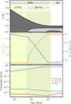 |
Fig. 1. Evolution of a 0.55 M⊙ model. Top: Kippenhahn diagram. Radius of interfaces in solar unit as a function of the model’s age. Convective zones (resp. radiative zones) are represented as dark (resp. light) gray areas. Middle: Aspect ratio (left axis) and density contrast (right axis). The inner radius, ri, is the bottom radius of the convective envelope, while the outer radius, ro, is 90% of the photospheric radius. Bottom: Kelvin-Helmholtz (blue) and convection (green) timescales and surface rotation period (red). The shaded areas correspond to the classical T Tauri phase (CTTS; light green), which coincides in our case with the disk-locking phase and weak T Tauri phase (WTTS; green). |
Figure 2 displays normalized gravity and angular velocity Ω profiles for three stages: the end of the CTTS phase (blue) and the middle (orange) and end (green) of the WTTS phase. For our 0.55 M⊙ model, the CTTS phase ends while the model is still fully convective and thus rotates as a solid body. When the star decouples from the disk and the radiative core appears, the radial differential rotation inside the radiative zone increases with time. The internal increase is predominantly controlled by contraction, despite the presence of shear-induced mixing and of meridional circulation that tend to smooth its effect. We note that a convective core temporarily formed at the end of the WTTS phase where (Fig. 1, top panel), also visible through the flat part of the Ω-profile in Fig. 2 (green)1. The normalized gravity profile, changes from a parabolic profile for the fully convective model to a hyperbolic one in the upper half of the stellar bulk once the radiative core appears and the matter gets more and more concentrated toward the center. This evolution of the model’s structure is also visible in the middle panel of Fig. 1, which shows the convective envelope’s aspect ratio ξ = ri/ro. Here, the inner radius ri is the radius at the bottom of the envelope while outer radius ro is taken as 90% of the total radius. This choice allowed us to focus on the adiabatic part of the envelope and neglect dramatic drops of density close to the surface2. We observed that the thickness of the radiative zone increases during the WTTS phase, so ξ increases until it reaches a plateau that will last during the entire MS. The density contrast Nρ ≡ log[ρ(ri)/ρ(ro)] in the convective envelope follows an inverse behavior: It decreases since most of the matter becomes concentrated in the central region. This counterintuitive trend results from the simultaneous outward migration of the base of the convective zone (i.e., the increase in ξ). For the very-low-mass star considered here, it goes from 4 to about 2.5. We note that for a solar mass, Nρ gets slightly lower values around 1.5.
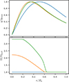 |
Fig. 2. Normalized gravitational acceleration g/gmax (top panel) and normalized angular velocity Ω/Ωsurf (bottom panel) as a function of the radius. These profiles are shown at the beginning (blue), middle (orange), and end (green) of the WTTS phase. Same model as in Fig. 1. |
The characteristic timescale of the PMS star is of the order of the global thermal (or Kelvin-Helmholtz) timescale τKH ≡ GM2/(RL), where G is the gravitation constant, and M, R and L are the stellar mass, radius and luminosity. This is the time necessary to radiate away the gravitational energy released during contraction. This timescale is always orders of magnitude larger than the period of rotation Prot or the convective turnover timescale τconv, which is provided by the mixing length theory (MLT) and integrated over the convective bulk. As shown by observations and simulations, the timescale associated with stellar convective dynamo is of the order of thousands of rotation periods only, so that we can safely neglect the variations of the radius and aspect ratio in these simulations. Moreover, in this figure, we also observed that the convective Rossby number averaged over the convective zone, representing the ratio Prot/τconv, tends to increase globally along the evolution on the PMS, going from about 0.01 to about 0.1. It is thus a good indicator of age on the PMS. We note, however, that this monotonic behavior can be slightly perturbed depending on the assumptions considered for the angular momentum redistribution (e.g., Amard & Matt 2023).
Finally, the very small predicted values of τconv are generally used as a justification for solid body rotation in convective zones, as assumed by Cesam2k20. This is, however, a rough simplification. In contrast physically grounded models (e.g., based on conservation of specific angular momentum) allow for decreasing rotation rate with radius in thick envelopes (e.g., Kissin & Thompson 2015). Contrary to Cesam2k20 assumption of a solid body rotating convective zone, radial differential rotation is certainly ubiquitous in PMS convective envelopes and mainly ruled by the rotation of the underlying radiative layers. This differential rotation evolves on a τKH timescale and thus can be considered as constant with respect to convective dynamos. Our aim is thus to study how this differential rotation affects dynamo in the convective layers using direct numerical simulations.
3. Dipole stability in sheared 3D DNS
In this section, we investigate the influence of an imposed radial differential rotation on dipolar dynamos driven by convection using DNS. We describe the numerical set-up of our 3D simulations, the influence of radial gravity profiles on convection, and the change in topology of magnetic fields with increasing differential rotation.
3.1. Numerical setup and choice of parameters
We solved the so-called anelastic dynamo model in MagIC software (Jones et al. 2011; Gastine & Wicht 2012), solving coupled equations of momentum, magnetic induction and entropy in spherical shells rotating with a surface rotation rate of Ωs. Convection is driven by the gradient of entropy imposed between the inner and outer spheres as Dirichlet boundary conditions. These surfaces are considered insulating to provide boundary conditions for magnetic field.
At the top and bottom boundaries of the shells, we assume no-slip conditions. In the frame corotating with the surface at angular velocity Ωs, we introduce a difference in rotation rate imposed between the inner and the outer spherical shell, ΔΩ, modeling the combined effects of the contraction-induced speed-up of the inner core, the surface angular momentum loss by magnetic interactions with the surroundings, and the transport of the angular momentum inside the star. This way, the angular velocity below the convective zone is Ωs + ΔΩ, with ΔΩ > 0. Even without imposed external differential rotation, i.e., ΔΩ = 0, weaker differential rotation naturally develops in convective dynamos as a result of momentum transport by convective turbulent motions and magnetic stresses. Its development is a nonlinear process, and is not taking into account external to convection processes (such as differential rotation of the radiative core and winds). Imposing differential rotation across the convection zone allowed us to model and control the impact of these processes on the stellar dynamo.
The two key governing parameters of the system are the shear Rossby number,
 (1)
(1)
and the (local) convective Rossby number, defined as
 (2)
(2)
and based on the convective length scale lconv(r). In the above equation, urms is the rms velocity of the flow, and Eℓkin(r) is the contribution of the spherical harmonic degree, ℓ, to the total kinetic energy, Ekin(r). If we average this quantity over radius, we get Roconvℓ, as defined in Christensen & Aubert (2006), which depends on the radially averaged characteristic length scale and rms velocity of the flow. While the shear Rossby number is the control parameter of our setup, the convective Rossby number is the diagnostic parameter, and it is not known a priori, i.e., before the simulation has been performed.
The Ekman number is set to Ek = 10−4, corresponding to moderately rotating stars, and the Prandtl number is set to Pr = 1. Although the latter quantities are much larger than values expected in stars, they are likely a valid choice if we consider the diffusivities of the simulations as effective turbulent coefficients (e.g., Bhattacharya et al. 2026). We restricted our simulations to layers between the bottom of the convective envelope at radius ri and the external radius ro located 10% of the actual stellar radius below the surface. Without loss of generality, the reference state of the simulations follow a polytropic structure (with a polytropic index n = 2). The density contrast is set to Nρ = 2.5, equivalent to an inner-to-outer density ratio of ρ(ri)/ρ(ro)≈12 typical of PMS stars (see Sect. 2). Furthermore, we vary radius (aspect) ratio ξ = ri/ro ∈ [0.1, 0.2, 0.35] to mimic the narrowing of the convective envelope during the PMS evolution. Magnetic Prandtl number is Pm ∈ [4, 6], and we employ several values of the Rayleigh number Ra to test more or less turbulent convective states. (See Appendix B for the definitions of these parameters.)
In addition to the evolutionary constraints on the density contrast and the aspect ratio, we also take into account changes in the gravity profile during the PMS evolution. As an illustration, Fig. 3a shows the normalized gravity profiles of a 0.8 M⊙ star at solar metallicity and at two different stages (see also Fig. 2 for a 0.55 M⊙ star). The gravity profile evolves from a quasi parabolic (e.g., 1 Myr T Tauri model with Nρ ≃ 1.7) to a predominantly hyperbolic one g ∝ 1/r2 (e.g., at the age of 4.9 × 10³ Myrs on the early MS, with Nρ ≃ 1.5). Regarding the very beginning of stellar formation, it is also interesting to consider the limiting case of a uniform density spherical shell, with the gravity increasing linearly with radius. Therefore, for sake of completeness, we explored three different profiles in our simulations: g ∝ r, g ∝ 1/r2, and a parabolic-like gravity profile typical of young PMS stars (i.e., around 1 Myr). The third profile is from the Cesam2k20 model in Fig. 3a and approximated with polynomials as a function of μ ≡ r/ro:
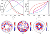 |
Fig. 3. Patterns of convection with different gravity profiles. (a) Normalized gravity profiles from stellar evolution code Cesam2k20 for a star of 0.8 M⊙ at an early stage of stellar evolution (1 Myr, in light gray) and at the MS (4.9 ⋅ 103 Myrs, dark gray). Example of imposed gravity profiles in DNS: g ∝ 1/r2 for radii ratio ξ = 0.35 (in red), g ∝ r and ξ = 0.2 (in dashed light blue) and a typical profile from Cesam2k20 with ξ = 0.35 (in magenta, see Eq. (3) for detail). (b) Local convective Rossby number, normalized with its maximum, as a function of r/ro for the runs gr2_2, gr_1, and gc_2, associated with the gravity profiles of panel (a) (same color code), and for the run gr2_3, with g ∝ 1/r2 and ξ = 0.2 (in dashed red). Details of the runs are presented in Table B.1. (c) Equatorial cut of instantaneous radial velocity for g ∝ 1/r2, ξ = 0.35 (run gr2_2). (d) Same as (c) but for g ∝ r, ξ = 0.2 (run gr_1). (e) Same as (c) but for g ∝ 1/r2, ξ = 0.2 (run gr2_3). Velocities in panels (c-e) were normalized with ν/(ro − ri), i.e., kinematic viscosity, ν, and the thickness of convective zone. |
 (3)
(3)
The initial conditions of our simulations correspond to dipolar dynamos already identified in Gastine et al. (2012), who already considered the effects of Ra and Nρ for two different aspect ratios on the stability of dipolar dynamos. Our parameter set is very similar except that we consider higher values of Pm to stabilize dipolar dynamos, as required by our higher (and more realistic) value of Nρ. We then impose a radial shear rate ΔΩ. Previous work show that differential rotation can give rise to different dynamical regimes in stably stratified spherical Couette flows under the effect of shear instability (Wicht 2014). Here, we limit our attention to low values of shear rates below the critical one for the shear instability; convection is thus the primary instability responsible for turbulent motions which are not considerably perturbed by the imposed shear, as can be seen from relatively unchanged radial distribution of Roconv in Fig. 4.
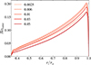 |
Fig. 4. Local convective Rossby number as a function of normalized radius, r/ro, for the typical values of Rosh considered in this work. The gravity profile is from Cesam2k20, approximated by Eq. (3). (See run gc_1 in Table B.1 for more details on the parameters.) |
3.2. Patterns of convection with different gravity profiles
In a preliminary step, it is worth discussing the impact of the stellar gravity profile evolution on the convective flow properties. First, in the limiting case of g ∝ r, as expected at very early stages of stellar formation (i.e., quasi uniform density), the convection seems more vigorous near the outer shell, as shown in Fig. 3d. For the same values of Nρ = 2.5 and ξ = 0.2, assuming this time g ∝ 1/r2, as expected for instance at the end of the PMS stage (i.e., matter is concentrated in the inner core), convective columns become very concentrated around the bottom boundary, as shown in Fig. 3e. Unsurprisingly, convective velocities are higher where gravity (and thus buoyancy driving) is maximum for such a relatively mild density contrast. We note that larger density contrasts would counteract the effect of a decreasing gravity profile and also favor convective motions in the very outer shells, similarly to a gravity profile g ∝ r (e.g., Gastine et al. 2012; Raynaud et al. 2014; Guseva et al. 2025). For a thinner convective shell (i.e., ξ = 0.35), we saw in Fig. 3c that the convective velocity is more homogeneously distributed in the convective bulk.
Dynamo action is promoted by helicity, which is directly correlated with the convective Rossby number. As seen in Eq. (2), the latter is proportional to the inverse of the convective characteristic length scale. In Fig. 3b, we plot the radial profiles of this quantity for different gravity profiles. In case g ∝ r, Roconv(r) has a clear maximum in the outer layers where the convective velocity is large and associated with small scales. In case g ∝ 1/r2, Roconv(r) is also maximum close to the surface, although more homogeneously distributed than in case g ∝ r. This statement holds true even in case ξ = 0.2, despite a maximum velocity close to the center, as seen in Fig. 3e. For a gravity profile comparable to that of Cesam2k20 PMS models, the Roconv(r) profile remains between the two previous limiting cases. This systematic increasing trend toward the surface mainly results from the sharp drop of density close the top boundary. This promotes very small scale motions and thus high values of Roconv(r) and helicity. As a result, we observed that the gravity profile only slightly affects the radial distribution of Roconv(r) and thus helicity. Because differences are small, dynamo mechanisms of large-scale field generation are thus expected to be universal for all gravity profiles, as we observed in Sect. 4.
3.3. Evolution of dipolarity and magnetic topology
Figure 5 shows the evolution of the axisymmetric radial component of the magnetic field, ⟨Br⟩ϕ, as a function of time and latitude for the most typical behaviors observed in our simulations. In the following, we quantify the dipolarity using the integral value,
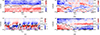 |
Fig. 5. Butterfly diagrams of the axisymmetric radial magnetic field component, ⟨Br⟩ϕ, together with the dipolarity. The term Ωst corresponds to the rotation time and follows the uniform rotation of a meridional plane. (a) Stable dipole for g ∝ 1/r2, Ra = 5 × 10⁶, ξ = 0.35, Rosh = 0.005. (b) Equatorially propagating dipolar waves for the same parameters, except for Rosh = 0.02. (c) Aperiodic dynamos for g ∝ 1/r2, Ra = 5 × 10⁵, ξ = 0.1, Rosh = 0.015. (d) Steady quadrupolar dynamos for g ∝ r, Ra = 1.6 × 10⁷, ξ = 0.2, Rosh = 0.3. The magnetic field was normalized with (ρoμ0λiΩs1/2), where ρo is the density at the outer boundary, λi is magnetic diffusivity at the inner boundary, and μ0 is the free space permeability. |
 (4)
(4)
comparing the energy concentrated in the ℓ = 1 dipolar modes and the energy of large-scale spherical harmonics up to a cutoff angular degree (ℓcut = 11 in this work).
When Rosh is weak, we conserve a stable dipole magnetic topology that does not vary in time, as seen in Fig. 5a for Rosh = 0.005. We note that the dipolarity slightly decreases in comparison to the nonperturbed case (i.e., Rosh = 0), yet it remains higher than 0.5. For the same gravity profile, g ∼ 1/r2 and slightly higher shear (i.e., Rosh = 0.02), the dipole becomes distorted. After the transition, dipolarity remains lower than 0.5, as the flow typically exhibits equatorward propagating waves (see Fig. 5b). We also sometimes observed sharper and erratic dipole-quadrupole transitions, as can be seen in Figs. 5c. Further increase in Rosh usually does not change this distribution of the magnetic field. When Rosh is very large and rotational dynamics dominate, we can nevertheless observe steady dipolar-quadrupolar solutions, with the dipole mostly concentrated around the tangent cylinder. Such solutions would be relevant only for very rapidly rotating stars, not low-mass PMS stars. They are therefore not represented here and not considered in the following sections.
3.4. Dipole collapse: Shear versus convection competition
The angular velocity distribution of our simulations with Rosh = 0 corresponds to a configuration with slow poles and fast equator or near-equator jets (e.g., Gastine & Wicht 2012). Thus, the local radial gradient of differential rotation, or local shear Rossby number,
 (5)
(5)
typically increases with radius, with the most pronounced increase at the tangent cylinder circumscribing the inner sphere (Fig. C.1a). Here, Ω = ⟨Uϕ⟩/r sin θ, where Uϕ is the azimuthal component of velocity in the frame corotating with angular velocity, Ωs, of the surface and ⟨⋯⟩ denotes the azimuthal average. The term Ω satisfies the boundary conditions in our simulations, i.e., Ω(ri) = ΔΩ, and Ω(r0) = 0. With a non-null imposed rotation, ΔΩ, all the area around the inner sphere rotates faster than the background rotation Ωs, developing a so-called Stewartson shear layer (Wicht 2014). This leads to suppression of positive differential rotation at this location and development of negative rotation gradients in the radial direction instead (Fig. C.1b). As Rosh increases, the shear becomes increasingly pronounced and extended in this region until the dipolar dynamo is disrupted (Figs. C.1c and d). This process can be seen as a competition between local shear expressed by Roshl(r) and convection, expressed by the (local) convective Rossby number Roconv(r), both of which vary with radius (e.g., Fig. 3b). Figure 6 shows the ratio of these two quantities for g ∼ 1/r2 and ξ = 0.35, corresponding to narrow convective zone, for several values of global Rosh, in the middle of the domain, ri/ro = 0.5 and as a function of latitude θ. As discussed above, we observed a clear correlation between the strength of the negative shear, developing at θ ∈ [30 − 40], and the collapse of the dipole (dashed lines), which takes place at Rosh ≈ 0.15 in this case. This result supports the idea that this ratio represents the appropriate parameter to characterize the dipole collapse.
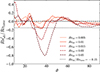 |
Fig. 6. Ratio of the local radial shear to the local convective Rossby number as a function of latitude (in degree) at the midgap, r/ro = 0.5, for varying Rosh. Solid lines denote stable dipolar states, with magnetic topology as depicted in Fig. 5a, and dashed lines denote collapsed dipoles as those depicted in Fig. 5b. |
To simplify and for future applications in one-dimensional stellar evolution codes (see example in Sect. 5), we seek instead for a criterion of the dipole collapse as a function of the total shear Rossby number, Rosh, as defined by Eq. (1), and the integrated in radius convective Rossby number Roconvℓ, obtained from the radial average of Eq. (2). Fig. 7a shows the time-averaged dipolarity of our models as a function of Rosh/Roconvℓ, as soon as the dynamo steady state is reached. We first saw that for a fixed aspect ratio ξ = 0.35 and for both the hyperbolic gravity profile and the realistic gravity profile from Cesam2k20, the transition from steady dipole toward dipolar oscillatory dynamos occurs at Rosh/Roconv ∼ 0.1, which is very close to the local value observed in Fig. 6. In addition, this threshold does not evolve when varying the Ra number. Figure 7b compares solutions for different envelope thickness (i.e., ξ = 0.1, 0.2 and 0.35). The thicker the envelope, the higher the critical value of Rosh/Roconv. Moreover, the transition seems to occur less abruptly at ξ = 0.2, that is, over a wider interval of values for Rosh/Roconv. In this interval, we observe reversing yet dipolar solutions with a seeming bi-stability with the steady dipole. For ξ = 0.1, the dipole collapse is even more delayed, with the flow first passing through a range of distorted states with slow evolution and no clear frequency, as those shown in Fig. 5c. These solutions eventually develop a periodic frequency and become oscillating waves for higher value of Rosh.
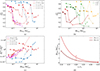 |
Fig. 7. Integral properties of the dynamo with increase of differential rotation. (a) Time-averaged dipolarity parameter as a function of the ratio between shear and convective Rossby numbers for Pm = 4 and three different gravity profiles: g(r) from CESAM in Eq. (3) in magenta, g ∝ 1/r2 in red, and g ∝ r in blue. The lines represent the following: solid lines, ξ = 0.35; dashed, ξ = 0.2; and dotted, ξ = 0.1. More (less) transparent lines correspond to the runs with a lower (higher) Ra number, for a fixed gravity profile and radius ratio (see Table B.1). The shapes represent the following: filled circles, stable dipoles (Fig. 5a); empty circles, reversing dipoles; diamonds, dipolar-quadrupolar waves (Fig. 5b); crosses, mixed dipolar and multipolar solutions without coherent temporal dynamics (Fig. 5c); and squares, equatorially symmetric solutions (Fig. 5d). (b) Same as in panel (a) but for g ∝ 1/r2 only and varying radius ratio. Light color, Pm = 4; dark color Pm = 6. Line styles and symbols as in panel (a). (c) Ratio of rms of axisymmetric toroidal and poloidal magnetic components Btaxi and Btaxi. Runs, lines, and symbols are the same as in panel (a). (d) Estimated critical collapse value of Rosh/Roconvℓ from all curves in panels (a) and (b), as a function of Pm and radius ratio ξ (stars) and the corresponding exponential fits (lines, Eq. 7). |
A particular case is the homogeneous mass distribution profile with g ∝ r in Fig. 7a (blue color). This case shows signs of bi-stability, with low values of Ra following the same trend observed with other gravity profiles for thin envelopes (i.e., ξ = 0.35), and high values of Ra leading to a very stable dipolar branch that is lost only for very strong values of Rosh toward a non-oscillatory, equatorially symmetric (quadrupolar) dynamo branch (Fig. 5d). We come back to this phenomena and discuss it in more detail when describing the mechanisms of dynamo collapse in the next section.
3.5. Increasing magnetic effects and criterion for dipole stability
Previous works highlighted that increasing magnetic Prandtl number tends to promote strong-field dipolar solutions and therefore stabilizes the dipole against multipolar, disordered solutions (Schrinner et al. 2014; Dormy 2016; Petitdemange 2018; Menu et al. 2020; Pinçon et al. 2024). In this work, we tested this effect to identify if it will increase the critical Rosh/Roconvℓ. Counterintuitively, we find that increasing Pm leads to slightly earlier destabilization of the dipole, for all tested radii (Fig. 7b), and at comparable values of Ra. Since in DNS Pm controls the strength of magnetic field, this result indicates that stars with stronger field (as, for example, measured by their Elsasser number), are more prone to lose their dipoles. A possible explanation for this behavior may result from a better coupling between the super-rotating inner core with the bulk flow. In other words, magnetic effects are likely to extend the influence of the differential rotation on a larger distance. We leave detailed investigation of this effect for the future work.
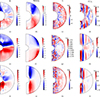 |
Fig. 8. Meridional distribution of the relevant dynamo properties. From left to right, the panels show the azimuthally averaged snapshots of the radial magnetic field component ⟨Br⟩; flow helicity H = ⟨U ⋅ ∇ × U⟩; the r component of the γ effect, which is axisymmetric by definition (6); and meridional circulation ⟨Ur⟩. All runs are without imposed differential rotation at the bottom of the convective zone (Rosh = 0). Top row (panels a–d): g ∝ 1/r2, Ra = 5 × 10⁶, and ξ = 0.35. Middle row (panels e–h): g ∝ r, and Ra = 8 × 10⁶, ξ = 0.2. Bottom row (panels i-l): g ∝ 1/r2, Ra = 1 × 10⁶, and ξ = 0.2. The dotted line corresponds to the considered latitude in the bottom panels of Figs. 9 and C.3. The γ effect and ⟨Ur⟩ are normalized using viscous units of the code (see Fig. 3); helicity is thus normalized by ν2/d3. Magnetic field units are the same as in Fig. 5. |
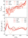 |
Fig. 9. Competition of the gamma effect with meridional circulation. Top: Radial component of the gamma effect γr as a function of Rosh (legend) averaged over colatitude, θ. Bottom: Radial component of meridional circulation near the equator (colatitude of θ = 80°, see Fig. 8d). Solid lines indicate that the dipole is stable; dashed lines show that the dipole has collapsed. The data are from the runs with g ∝ 1/r2, Ra = 5 × 10⁶, and ξ = 0.35 (gr2_2 in Table B.1). Subscripts ϕ and θ denote azimuthal and latitudinal average, respectively. The units are the same as in Figs. 3(c–e). |
4. Mechanisms of dipole collapse
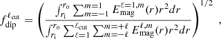
We interpret the mechanisms of the destabilization of dipoles in our simulations from the viewpoint of dynamo theory. The broken symmetry of rotating convective turbulence is expected to drive axisymmetric fields due to nonzero correlation between flow velocity and vorticity (α effect). In addition, high anisotropy of convective structures leads to systematic advection redistributing magnetic field across the domain (γ effect). Differential rotation, which develops due to turbulent momentum mixing, stretches poloidal field lines intro toroidal fields lines (ω effect). All of these processes, which are opposed by turbulent diffusion (ηT), support large-scale magnetic fields, according to the mean-field dynamo equations:
![Mathematical equation: $$ \begin{aligned} \frac{\partial \mathbf \langle \boldsymbol{B} \rangle }{\partial t} = \nabla \times \left( \left[\langle \boldsymbol{U} \rangle + \boldsymbol{\gamma } \right] \times \langle \boldsymbol{B} \rangle + \alpha \langle \mathbf B \rangle - \eta _T \nabla \times \langle \boldsymbol{B} \rangle \right). \end{aligned} $$](/articles/aa/full_html/2026/03/aa57616-25/aa57616-25-eq6.gif) (6)
(6)
Vector γ can be interpreted as being an additional axisymmetric mean-field advection velocity in Eq. (6), and it is in addition to the axisymmetric mean flow ⟨U⟩. The final magnetic configuration depends on the balance between these processes. Vector γ and tensor α can be computed directly from 3D data using the Singular Value Decomposition (SVD) inversion method of Simard et al. (2016), as was done in this work.
4.1. Induced ω effect
Guided by general transitions of dipolar dynamos to oscillatory solutions, the need of high differential rotation and corresponding radial shear in Fig. C.1 to trigger dipole collapse hints toward a transition from α2 to α2ω dynamos and excitation of oscillatory dipolar branches. Such transitions are typically accompanied by an increase in the toroidal component of magnetic field, which is stretched out by the differential rotation. To test this hypothesis, we plot the ratio between the rms values of the axisymmetric toroidal and poloidal components of magnetic field, integrated over the entire domain, in Fig. 7(c). For most of the models, this ratio remains relatively constant for stable dipolar solutions at small Rosh. As a general trend, it gradually increases as soon as periodic dipolar waves develop. This increase is stronger for thinner convective zones (ξ = 0.35) and less pronounced for thicker ones (ξ = 0.1), where wave onset is delayed. The fact that this increase is slow, and not abrupt, hints at gradual, supercritical transition between steady and oscillatory dipolar dynamo branches during dipole collapse. In contrast to that, the transition to quadrupoles at g ∝ r and high Ra number is abrupt and thus potentially subcritical. We plan to investigate the bifurcation scenarios of these dynamo branches in more details in the future work.
4.2. Disruption of the γ effect
In the simulations with ξ = 0.35, g ∝ 1/r2, and with gravity profile in Eq. (3) from Cesam2k20, the dynamo action takes place predominantly outside the tangent cylinder and occupies nearly homogeneously the bulk of the flow (Fig. 8b). Although the peak of magnetic energy is located inside the tangent cylinder, the large-scale dipole is occupying the entire domain (Fig. 8a). As Rosh increases, we did not find a strong systematic modification in helicity distribution or radial dependence of Roconv number (Fig. 4), and thus imposed levels of rotation do not disturb significantly the length scale and magnitude of convective columns and generated by them α effect. Similarly for γ effect, it remained nearly unmodified in this set of simulations, with the radial component γr showing inward pumping of magnetic energy in the bulk of the flow, and the outward direction of this component at the outer sphere. This distribution of γr has been shown to have an important role in supporting dipolar dynamos, by re-distributing magnetic flux from the areas where toroidal field is generated, to the areas of poloidal field, providing additional exchange for the two field components (Schrinner et al. 2012). When γr is small, dipolar dynamos ceased to exist and gave way to multipolar periodic fields. Decrease in efficiency of the γ effect due to differential rotation could be one of the causes of the dipole collapse. However, our simulations do not exhibit strong variations in γr as a function of Rosh, as shown in Fig. 9 (top panel). There, the radial distribution of γr, integrated over latitude θ, remains predominantly negative at lower radii and predominantly positive at higher radii, for both dipolar and nondipolar runs.
On the other hand, due to mass and momentum conservation, imposed differential rotation leads to enhancement of poloidal (meridional) mean flows. Although in our simulations they have quite complex, multi-cellar topology corresponding to at least two large recirculation zones, all the runs feature an area of positive mean radial velocity ⟨Ur⟩ϕ (Fig. 8d) developing near the equator and tangent cylinder. As Rosh increases, the strength of this radial velocity becomes progressively larger (Fig. 9b). This velocity component, as seen from Eq. (6), thus opposes negative magnetic pumping in the bulk of the domain and contributes to destabilization of the dipolar field component.
4.3. Influence of the gravity profile
The homogeneous profile g ∼ r results in mean magnetic field concentrated around the equator (Fig. 8e). Intensity of convective columns is the largest near the outer boundary (Fig. 3d), which implies the concentration of flow helicity H = ⟨U ⋅ ∇ × U⟩ in the bulk at large radii (Fig. 8f). The generation of magnetic field is thus located in this narrow zone, which has to be disturbed to obtain dipole collapse. Thus, the empirical local criteria for relation between the shear and convective Rossby numbers, such as those in Fig. 6, are satisfied in the outer layers (r/ro ≈ 0.9), and not in the bulk of the flow. On the other hand, the relative topology of the γ effect, although weakened in comparison to g ∼ 1/r2 profile, remains similar, with an area of negative radial mean flux of magnetic energy (Fig. 8g), and strengthening of the meridional flow at the tangent cylinder in comparison to γr (Fig. C.3a). Our results suggest that this gravity profile exhibits delay in dipole collapse due to location of the bulk of helicity outside of the zone of strong shear. For higher Ra number, the dipole is overstable, and drops on a entirely different, equatorially symmetric dynamo branch (Fig. 5d). We leave detailed study of stability of this gravity profile for the future work. Since it is relevant for stars just at the beginning of their formation and not on the PMS, we do not take it into account when deriving a more general shear criterion for dipole collapse on the PMS.
4.4. Impact of convective zone thickness
In simulations with wider convective shells, ξ = 0.1 or 0.2, the bulk of helicity is located in deeper layers than for ξ = 0.35 (compare Figs. 8j and b), following the location of convective columns (Fig. 3e). The dynamo is thus “deep-seated" at the bottom of convective zone, with magnetic energy decaying with radius (Fig. 8i). The magnetic fields of these dynamo solutions are “weaker” and typically have lower Elsasser numbers (see Table B.1); stronger fields at higher levels of turbulence result multipolar in this parameter regimes, even without imposed radial differential rotation. In addition, the topology of the radial γ effect considerably changes, developing weak but predominantly positive advection in the equatorial regions, repelling magnetic flux outward. At high latitudes, the distribution of γr appears noisy and small-scale (Fig. 8k), and the radial direction of θ-integrated magnetic pumping (Fig. C.3b) is overall neither negative nor positive. However, the latitudinal component γt shows the same topology as in previous cases (compare panels a, b, and c in Fig. C.2), but shifted inward, similar to the distribution of helicity. This indicates that magnetic flux is still potentially generated and transported inward at high latitudes inside the tangent cylinder, even if this is not obvious in Figs. 8 and C.3 due to the noise. The area of magnetic pumping thus partially bypasses the region of negative shear, developing due to rotation (like that in Figs. C.1b–d). Thus, although meridional circulation is also enhanced at the tangent cylinder (Fig. C.3b, bottom), it affects the mean-field dynamo process less, and therefore dipole collapse is delayed, resulting in dipole reversals first. In addition, the location of negative shear region in the middle of dynamo-generating zone implies that the product of α∇Ω, defining the direction of the waves (Yoshimura 1975; Tobias 2021), changes sign across the dynamo-generating area. This may explain why the dynamo falls first on aperiodic solutions without well-defined frequency at ξ = 0.1 (Figs. 7a,b), before developing oscillating dynamos.
5. Discussion on stellar applications
5.1. Fitting the dipole collapse threshold in DNS
For practical stellar applications, it can be useful to obtain a simple ad hoc expression for the critical value of Rosh/Roconvℓ above which dipoles collapse as a function of the aspect ratio ξ. Indeed, ξ is representative of the internal structure of PMS stars and globally increases with age (see Sect. 2). To derive such an expression, we estimate the values of Rosh/Roconvℓ before and after collapse at a given ξ value, and compute the mean value. In Fig. 7d we plot these mean values as a function of ξ = ri/ro, for Pm = 4 and 6. The solid lines correspond to exponential fits to these critical mean thresholds in the form of C(Pm)exp(−βξ),
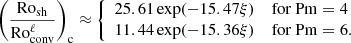 (7)
(7)
The dependence on ξ in the exponent function is the same for both of the considered Pm values. Varying Pm modifies only the pre-factor. While for thick shells, ξ = 0.1, the dipole is two times more stable at Pm = 4. This difference becomes smaller as ξ increases and is nearly negligible around ξ = 0.35. The last criterion thus tends to become independent of Pm around ξ ∼ 0.35, that is, the dipole stability is expected to be less dependent on the relative strength of stellar magnetic field (increasing with Pm). The collapse threshold (Rosh/Roconvℓ)c ∼ 0.1, valid for ξ = 0.35, can thus be seen as a limiting ratio. All stars with convective zones thinner than this one can be assumed to have their dipoles collapsed if Rosh/Roconvℓ ≳ 0.1. We assume this in Sect. 5.3. We plot in Fig. 10 the dipolarity as a function of Rosh/Roconvℓ normalized by its critical value taken from Eq. (7). This figure perfectly illustrates the shear-induced dipole collapse identified in this work.
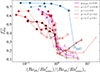 |
Fig. 10. Data for time-averaged dipolarity from all runs of this paper as a function of compensated shear Rossby number (i.e., Rosh/Roconvℓ) and normalized by its critical value given in Eq. (7). All transitions from dipolar to oscillatory branches collapse on each other. The branch that does not follow the trend is the special case of g ∝ r and the high Ra values (run gr_2 in Table B.1, see Fig. 5d and discussion in Sect. 4.3). Colors, symbols, and lines are the same as in Fig. 7. |
5.2. Estimate of the Rossby numbers in 1D stellar evolution models
The expression of the shear Rossby number Rosh in Eq. (1) is not straightforward to translate into 1D stellar models. First, the radial shear ΔΩ entering Rosh has no equivalent in a Cesam2k20 model, as the convective zone is assumed to rotate as a solid body. Nevertheless, this is certainly not true in stars, where a degree of shear should exist close to the boundary with the radiative core (see Sect. 2). Therefore, on the one hand, we estimated an inner angular velocity, Ωi, as the angular velocity in the radiative zone (denoted as “RZ”) averaged with its moment of inertia:
 (8)
(8)
On the other hand, one may argue that the effect of the angular velocity of the very deep regions of the radiative zone on the stability of the dipole is negligible compared to that of the angular velocity close to the convective boundary. It then seems reasonable to consider the value of Ω at a pressure scale height below the bottom of the convective zone rCZ − Hp, which defines Ωi, Hp.
Second, for the convective Rossby number Roconvℓ, the radial mean of Eq. (2), can be estimated in evolution models using the MLT convective velocity, vconv. Provided the global turnover timescale is τconv = ∫CZdr/vconv, it is straightforward to define a first global quantity Roconv, glob = 1/(ΩCZτconv). However, MLT fails to describe the very near surface layers which could bias this estimate. In the following, we thus prefer to consider Roconv, mid = vconv(rmid)/[ΩCZlMLT(rmid)], computed at the middle of the convective zone r = rmid, with the associated mixing length lMLT.
With these definitions, one can compute two different estimates of Rosh/Roconvℓ, which are more or less favorable to the stability of the dipole. Figure 11 shows variation of some of these ratios for a few evolutionary tracks. As the current description of angular momentum transport notoriously lack efficiency, we have considered for each track an additional turbulent viscosity νadd = 0, 104 and 106 cm2 s−1 in the radiative layers. This maximum value is compatible with the potential, still debated, transport by magnetohydrodynamic instabilities (e.g., Eggenberger et al. 2005, for a solar model). We saw that Rosh, glob/Roconv, mid is generally much larger than Rosh, Hp/Roconv, mid, as expected since the fast core rotation contributes to the value of Rosh, glob positively. This difference decreases as νadd increases, since the rotation profile gets smoother and smoother. In both cases, the dipole collapse criterion provided by Eq. (7) for Pm = 4 is met at the very beginning of the PMS evolution (i.e., around 1 Myr) if νadd is below a threshold value: the lower the mass, the lower the threshold value for νadd. We suggest that the ratio Rosh, Hp/Roconv, mid, based on the rotation in upper layers of radiative zone adjacent to CZ, is the more consistent with the results of the 3D simulations, where ΔΩ is imposed at the bottom of the CZ. Moreover, if its value is higher than the critical value for dipole collapse, this is also the case for Rosh, glob/Roconv, ensuring a conservative approach.
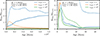 |
Fig. 11. Evolution with stellar age of the ratios Rosh, Hp/Roconv, mid (solid lines) or Rosh, glob/Roconv, mid (dashed lines). The color corresponds to the additional viscosity considered for the angular momentum transport. The dotted black line corresponds to the threshold defined in Eq. (7) for Pm = 4, with a minimum value of 0.1. Each panel corresponds to a given evolutionary track, whose initial parameters are given in each plot. |
5.3. Dipole stability through evolution
Using the parameter Rosh, Hp/Roconv, mid and the criterion in Eq. (7), we can explore the stability of an initial dipole during the PMS. To that end, we construct three grids (for νadd = 0, 104 and 106 cm2 s−1, see Sect. 5.2) of 700 stellar evolutionary tracks using the code Cesam2k20 (see Sect. 2.1), with different initial conditions. hence, one track corresponds to a series of structure models with same initial mass, Pdisk and τdisk, but different ages. Tracks in each grid have a mass between 0.3 and 1.3 M⊙, Pdisk between 6 and 10 days and τdisk between 1 and 10 Myrs, chosen following a Sobol’ pseudo-random algorithm (Sobol’ 1967; Bratley & Fox 1988). This choice avoids spurious patterns appearing in the final distributions. Because we are interested in early phases, each track is started in the CTTS phase, until the beginning of the MS phase (when 10% of the initial hydrogen content is consumed). An illustration of the evolution of the surface rotation period of these models can be found in Appendix D, Fig. D.1.
We then compare Rosh, Hp/Roconv, mid to the critical threshold for dipole collapse in Eq. (7) (for Pm = 4 and a minimum value equal to 0.1) over the stellar models grids. For each of the grids, we randomly chose five models per track. This is done to improve the readability of the distribution, and does not affect our conclusion thanks to the still large number of models considered. Fully convective models, i.e., M ≲ 0.35 M⊙, are not considered. We also reject models with an age below τdisk because that may introduce spurious patterns in our distributions (i.e., two models of the same track still coupled to the disk will be at the same place in the mass-period diagram). Figure 12 represents in red the models that have lost their dipole in their past life and in green, the one that maintained it. These distributions are mainly bimodal with a group for PMS (small periods; circles) and a group for the MS stars (long period; stars). Whatever the value of the additional viscosity is, there are few models that keep their initially stable dipolar field. Their number increases when νadd increases, incorporating older and older models. For νadd ≲ 104 cm2 s−1, a few stable dipoles are found but almost only in PMS models, while when νadd ≳ 106 cm2 s−1, many MS models have managed to keep it. We also notice a strong correlation with the mass of the model. The more massive models generally have a stronger increase of the angular velocity during initial contraction than less massive ones, which results in a higher Rosh, Hp (see Fig. 11).
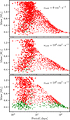 |
Fig. 12. Mass-period (surface) distribution of some models randomly chosen in the grids described in Sect. 5.3. The criterion considered for the stability of the dipole is the ratio Rosh, Hp/Roconv, mid with the threshold expressed in Eq. (7). Circles and stars are respectively PMS and MS models. Red (resp. green) markers are models that lost (resp. kept) their dipole between their formation and their present age. Each panel corresponds to a grid with a given additional turbulent viscosity, νadd. |
In case νadd ≳ 106 cm2 s−1, the predicted distribution of magnetic topology with mass on the MS qualitatively reproduces the mean observed trends, with dipolar (mostly poloidal) state for masses 0.35 M⊙ ≲ M ≲ 0.5 M⊙ and a transition toward more complex (toroidal) configurations for more massive low-mass stars (e.g., Donati & Landstreet 2009; Moutou et al. 2017; Donati et al. 2023). This suggests that the distribution of magnetic fields with mass on the MS for masses M ≳ 0.35 M⊙ is likely to result from a (still unknown) internal angular momentum redistribution process in the radiative core whose efficiency is such that the induced radial differential rotation can destabilize dipoles only for masses M ≳ 0.5 M⊙. Although less obvious, the distribution with mass on the PMS somehow shows similarities too (Nicholson et al. 2021). This observed behavior is of course dependent of the way we model the accretion and PMS phases and on the assumptions made for the evolution of magnetic fields (here, the dipole is assumed to be lost forever after its collapse). Future studies are needed to tackle these questions, out of scope of this work.
6. Conclusions
Large-scale differential rotation developing in thick convective layers of PMS stars can perturb the stability of their strong initial dipolar fields. In this work, we developed 3D numerical dynamo models of this process with imposed shear rates not significantly perturbing convection and well below the threshold for shear instability, which could also affect the field. We show that the key parameter for the stability of dipolar dynamos of PMS stars is the relative importance of a shear-based Rossby number compared to the convective Rossby number (see Figs. 7 and 10). Surprisingly, even relatively weak values of this ratio can lead to dipole collapse.
We considered different and more or less realistic gravity profiles in our 3D DNS affecting the location of turbulent motions (see Figs. 2 and 3), which could correspond to PMS stars at different ages. In general, the convective Rossby number is radially dependent (Fig. 2b), as observed in strongly stratified DNS (Raynaud et al. 2015). While it is instructive to explore local criteria for dipole stability (Fig. 6), such criteria cannot be used in 1D stellar evolution codes such as Cesam2k20, where the access to the 2D distribution of shear and convection is not available. We thus developed a criterion for dipole collapse based on the radially averaged value of the convective Rossby number and the total shear applied to the convective zone (Eq. (7)). Eventually, this ratio depends on the thickness of the convective zone, converging to a universal behavior as the star evolves and the zone becomes thinner (Fig. 7b). Our simulations with stronger magnetic effects (higher Pm) also require a slightly modified criteria (see also Menu et al. 2020; Zaire et al. 2022). However, a more extensive parameter study with a higher Pm is needed to explore magnetostrophic regimes in which the Lorentz force enters the dominant force balance (Dormy 2016) and to determine a relevant scaling law for the stability criteria as a function of magnetic field strength (or Pm).
Close to the transition between dipolar and oscillatory dynamos, the differential rotation does not significantly affect the distribution of the convective Rossby number (Fig. 4). Thus, it also does not affect helicity distribution in the flow for varying Rosh (not shown here). Helicity is strongly linked with the α effect in the dynamo theory, i.e., conversion from toroidal magnetic fields into large-scale poloidal ones, so this result suggests that the α effect is not affected by differential rotation. In contrast, increasing the imposed shear promotes toroidal magnetic fields generated by differential stretching of poloidal field lines (the ω effect; see Fig. 7c), and it affects the γ effect, which is the transport mechanism of particular importance for dipolar dynamos (see Figs. 9 and C.2, and Schrinner et al. 2012). The differential rotation governs the dynamo behavior beyond the critical values for collapse, with a consistent migration of radial fields toward the equator in agreement with Parker theory; i.e., the propagation direction depends on the sign of the radial differential rotation (Parker 1955; Schrinner et al. 2011). The appearance of more complex field morphologies and temporal evolution, such as aperiodic reversals and quadrupoles (Figs. 5c,d), suggest a potential bi-stability of different dynamo branches.
Finally, we adapted this criterion for the 1D stellar evolution code Cesam2k20, estimating the ratio of the shear-based Rossby number and the convective one during the evolution of stars, as shown in Fig. 11. We estimated whether the dipole collapsed or not during the PMS phase for random distributions of stellar models, which were constructed to mimic observations. Our results show that the redistribution of angular momentum taking place during the PMS phase can destabilize dipolar fields inherited from the proto-stellar phase and give rise to the diversity of magnetic topologies observed for MS stars (see Fig. 12), when strong turbulent viscosity in the radiative zone is considered. Our results thus provide an additional hint for more efficient transport of angular momentum in radiative zones of stars than provided by shear or meridional currents alone. The Sun, with its relatively large mass, moderate rotation, and cyclic, oscillatory magnetic field qualitatively fits well in the scenario of steady dipolar dynamo collapse and transition to oscillatory dynamos, as observed in this work.
Additional numerical studies are needed to determine if dipolar dynamos can be generated from oscillatory dynamos when shear flows decrease during the beginning of the MS phase. Moreover, to extrapolate these results to more massive stars, more sophisticated 3D DNS with adjacent stable and thermally unstable regions must be dynamically modeled.
Acknowledgments
The authors acknowledge financial support from the French program ‘PROMETHEE’ (Protostellar Magnetism: Heritage vs Evolution) managed by Agence Nationale de la Recherche (ANR), and would like to thank E. Alecian and the PROMETHEE team for inspiring discussions that helped to shape this work. This work was supported by the “Action Thématique de Physique Stellaire” (ATPS) of CNRS/INSU PN Astro co-funded by CEA and CNES, and the HPC facility MesoPSL for the computational resources. L. M. acknowledge support from the Agence Nationale de la Recherche (ANR) grant ANR-21-CE31-0018.
References
- Aikawa, M., Arai, K., Arnould, M., Takahashi, K., & Utsunomiya, H. 2006, AIP Conf. Ser., 831, 26 [Google Scholar]
- Amard, L., & Matt, S. P. 2023, A&A, 678, A7 [NASA ADS] [CrossRef] [EDP Sciences] [Google Scholar]
- Argiroffi, C., Caramazza, M., Micela, G., et al. 2016, A&A, 589, A113 [NASA ADS] [CrossRef] [EDP Sciences] [Google Scholar]
- Asplund, M., Grevesse, N., Sauval, A. J., & Scott, P. 2009, ARA&A, 47, 481 [NASA ADS] [CrossRef] [Google Scholar]
- Bhattacharya, S., Krasnov, D., Pandey, A., Gotoh, T., & Schumacher, J. 2026, J. Fluid Mech., 1026, A6 [Google Scholar]
- Böhm-Vitense, E. 1958, Z. Astrophys., 46, 108 [Google Scholar]
- Bouvier, J., Forestini, M., & Allain, S. 1997, A&A, 326, 1023 [NASA ADS] [Google Scholar]
- Bouvier, J., Matt, S. P., & Mohanty, S. 2014, Protostars and Planets VI, 433 [Google Scholar]
- Bratley, P., & Fox, B. L. 1988, ACM Trans. Math. Softw., 14, 88 [Google Scholar]
- Broggini, C., Bemmerer, D., Caciolli, A., & Trezzi, D. 2018, Prog. Part. Nucl. Phys., 98, 55 [CrossRef] [Google Scholar]
- Brun, A. S., Strugarek, A., Noraz, Q., et al. 2022, ApJ, 926, 21 [NASA ADS] [CrossRef] [Google Scholar]
- Christensen, U. R., & Aubert, J. 2006, Geophys. J. Int., 166, 97 [NASA ADS] [CrossRef] [Google Scholar]
- Donati, J. F., & Landstreet, J. D. 2009, ARA&A, 47, 333 [Google Scholar]
- Donati, J. F., Lehmann, L. T., Cristofari, P. I., et al. 2023, MNRAS, 525, 2015 [CrossRef] [Google Scholar]
- Dormy, E. 2016, J. Fluid Mech., 789, 500 [NASA ADS] [CrossRef] [Google Scholar]
- Eggenberger, P., Maeder, A., & Meynet, G. 2005, A&A, 440, L9 [NASA ADS] [CrossRef] [EDP Sciences] [Google Scholar]
- Ferguson, J. W., Alexander, D. R., Allard, F., et al. 2005, ApJ, 623, 585 [Google Scholar]
- Gallet, F., & Bouvier, J. 2013, A&A, 556, A36 [NASA ADS] [CrossRef] [EDP Sciences] [Google Scholar]
- Garraffo, C., Drake, J. J., & Cohen, O. 2016, A&A, 595, A110 [NASA ADS] [CrossRef] [EDP Sciences] [Google Scholar]
- Gastine, T., & Wicht, J. 2012, Icarus, 219, 428 [Google Scholar]
- Gastine, T., Duarte, L., & Wicht, J. 2012, A&A, 546, A19 [NASA ADS] [CrossRef] [EDP Sciences] [Google Scholar]
- Getman, K. V., Feigelson, E. D., & Garmire, G. P. 2023, ApJ, 951, 15 [NASA ADS] [CrossRef] [Google Scholar]
- Guervilly, C., & Cardin, P. 2010, Geophys. Astrophys. Fluid Dyn., 104, 221 [NASA ADS] [CrossRef] [Google Scholar]
- Guseva, A., Petitdemange, L., & Pinçon, C. 2025, A&A, 699, A68 [NASA ADS] [CrossRef] [EDP Sciences] [Google Scholar]
- Hartmann, L., Herczeg, G., & Calvet, N. 2016, ARA&A, 54, 135 [Google Scholar]
- Henyey, L., Vardya, M. S., & Bodenheimer, P. 1965, ApJ, 142, 841 [Google Scholar]
- Hill, C. A.& MaTYSSE Collaboration. 2017, IAU Symp., 328, 101 [Google Scholar]
- Hubeny, I., & Mihalas, D. 2014, Theory of Stellar Atmospheres: An Introduction to Astrophysical Non-Equilibrium Quantitative Spectroscopic Analysis (Princeton University Press) [Google Scholar]
- Iglesias, C. A., & Rogers, F. J. 1996, ApJ, 464, 943 [NASA ADS] [CrossRef] [Google Scholar]
- Jones, C., Boronski, P., Brun, A., et al. 2011, Icarus, 216, 120 [Google Scholar]
- Käpylä, P. J., Browning, M. K., Brun, A. S., Guerrero, G., & Warnecke, J. 2023, Space Sci. Rev., 219, 58 [CrossRef] [Google Scholar]
- Kissin, Y., & Thompson, C. 2015, ApJ, 808, 35 [NASA ADS] [CrossRef] [Google Scholar]
- Kunitomo, M., Guillot, T., Ida, S., & Takeuchi, T. 2018, A&A, 618, A132 [NASA ADS] [CrossRef] [EDP Sciences] [Google Scholar]
- Manchon, L., Deal, M., Marques, J., & Lebreton, Y. 2025, A&A, 704, A79 [Google Scholar]
- Marques, J. P., Goupil, M. J., Lebreton, Y., et al. 2013, A&A, 549, A74 [NASA ADS] [CrossRef] [EDP Sciences] [Google Scholar]
- Mathis, S., Prat, V., Amard, L., et al. 2018, A&A, 620, A22 [NASA ADS] [CrossRef] [EDP Sciences] [Google Scholar]
- Matt, S. P., Brun, A. S., Baraffe, I., Bouvier, J., & Chabrier, G. 2015, ApJ, 799, L23 [Google Scholar]
- Menu, M. D., Petitdemange, L., & Galtier, S. 2020, Phys. Earth Planet. Inter., 307, 106542 [CrossRef] [Google Scholar]
- Moffatt, H. K. 1978, Magnetic Field Generation in Electrically Conducting Fluids (University Press) [Google Scholar]
- Moraux, E., Artemenko, S., Bouvier, J., et al. 2013, A&A, 560, A13 [NASA ADS] [CrossRef] [EDP Sciences] [Google Scholar]
- Morel, P. 1997, A&AS, 124, 597 [NASA ADS] [CrossRef] [EDP Sciences] [Google Scholar]
- Morel, P., & Lebreton, Y. 2008, Ap&SS, 316, 61 [Google Scholar]
- Moutou, C., Hébrard, E. M., Morin, J., et al. 2017, MNRAS, 472, 4563 [NASA ADS] [CrossRef] [Google Scholar]
- Mueller, M. A., Johns-Krull, C. M., Stassun, K. G., & Dixon, D. M. 2024, ApJ, 964, 1 [Google Scholar]
- Nicholson, B. A., Hussain, G., Donati, J. F., et al. 2021, MNRAS, 504, 2461 [NASA ADS] [CrossRef] [Google Scholar]
- Parker, E. N. 1955, ApJ, 122, 293 [Google Scholar]
- Petitdemange, L. 2018, Phys. Earth Planet. Inter., 277, 113 [CrossRef] [Google Scholar]
- Petitdemange, L., Marcotte, F., Gissinger, C., & Daniel, F. 2024, A&A, 681, A75 [NASA ADS] [CrossRef] [EDP Sciences] [Google Scholar]
- Pinçon, C., Petitdemange, L., Raynaud, R., et al. 2024, A&A, 685, A129 [NASA ADS] [CrossRef] [EDP Sciences] [Google Scholar]
- Raynaud, R., Petitdemange, L., & Dormy, E. 2014, A&A, 567, A107 [NASA ADS] [CrossRef] [EDP Sciences] [Google Scholar]
- Raynaud, R., Petitdemange, L., & Dormy, E. 2015, MNRAS, 448, 2055 [NASA ADS] [CrossRef] [Google Scholar]
- Rogers, F. J., & Iglesias, C. A. 1992, ApJ, 401, 361 [NASA ADS] [CrossRef] [Google Scholar]
- Rogers, F. J., & Nayfonov, A. 2002, ApJ, 576, 1064 [Google Scholar]
- Scholz, A., Coffey, J., & Brandeker, A. 2007, ApJ, 662, 1254 [Google Scholar]
- Schrinner, M., Petitdemange, L., & Dormy, E. 2011, A&A, 530, A140 [NASA ADS] [CrossRef] [EDP Sciences] [Google Scholar]
- Schrinner, M., Petitdemange, L., & Dormy, E. 2012, ApJ, 752, 121 [NASA ADS] [CrossRef] [Google Scholar]
- Schrinner, M., Petitdemange, L., Raynaud, R., & Dormy, E. 2014, A&A, 564, A78 [NASA ADS] [CrossRef] [EDP Sciences] [Google Scholar]
- Simard, C., Charbonneau, P., & Dubé, C. 2016, AdSpR, 58, 1522 [Google Scholar]
- Sobol’, I. 1967, USSR Comput. Math. Math. Phys., 7, 86 [Google Scholar]
- Talon, S., Zahn, J. P., Maeder, A., & Meynet, G. 1997, A&A, 322, 209 [NASA ADS] [Google Scholar]
- Tobias, S. 2021, J. Fluid Mech., 912, P1 [Google Scholar]
- Venuti, L., Bouvier, J., Cody, A. M., et al. 2017, A&A, 599, A23 [NASA ADS] [CrossRef] [EDP Sciences] [Google Scholar]
- Wicht, J. 2014, J. Fluid Mech., 738, 184 [Google Scholar]
- Wright, N. J., Drake, J. J., Mamajek, E. E., & Henry, G. W. 2011, ApJ, 743, 48 [Google Scholar]
- Yamashita, M., Itoh, Y., & Takagi, Y. 2020, PASJ, 72, 80 [NASA ADS] [CrossRef] [Google Scholar]
- Yoshimura, H. 1975, ApJ, 201, 740 [Google Scholar]
- Zaire, B., Jouve, L., Gastine, T., et al. 2022, MNRAS, 517, 3392 [NASA ADS] [CrossRef] [Google Scholar]
The short appearance of a convective core, preceding ignition of H1 burning, corresponds to the first steps of CNO cycle. The chain of reactions, corresponding to 14N(p, γ)15O 12C(p, γ)13N(,β+ν)13C(p, γ)14N, stops when these elements are at equilibrium. The energy production rate is proportional to T19, destabilizing the medium and creating a convective zone.
Large-scale 3D numerical simulations as performed in Sect. 3 generally neglect these surface layers for numerical sobriety.
Appendix A: Physical ingredients of Cesam2k20 models
Main physical ingredients used in the Cesam2k20 models computed for this work.
Appendix B: Parameters and initial conditions for 3D simulations
The DNS code MagIC uses a set of dimensionless parameters that allow for control of the physical properties of our simulations. The ratio of viscous to Coriolis forces is Ekman number E = ν/Ωsd2 = 10−4, where ν is hydrodynamic viscosity, d = ro − ri the gap between the two spheres, and Ωs is the angular velocity of the surface (i.e., of the rotating frame). Furthermore, the density contrast Nρ = ln(ρi/ρo) = 2.5 allowed us to take into account the drop of density, ρ, across the convective zone. Prandtl and magnetic Prandtl numbers, Pr = ν/κ = 1 and Pm = ν/η, where η is magnetic diffusivity and κ thermal diffusivity, define diffusive properties of the fluid. Rayleigh number Ra = (GMdΔS)/(νκcp), where cp heat capacity, G gravitational constant, and M the central mass, controls the strength of convection (see Table B.1 for Pm and Ra). Table B.1 also shows diagnostic parameters that allow for comparison of our simulations with existing literature. Among them are the Elsasser, Reynolds, and Nusselt numbers:
 (B.1)
(B.1)
where Urms and Brms are the root-mean-square velocity and magnetic field, T is temperature, S entropy, c1 and ζi are functions of the polytropic reference state, and μ0 is the permeability of the free space. We refer the reader to the previous works (i.e., Guseva et al. (2025), Jones et al. (2011), Dormy (2016)) for a detailed discussion of these parameters.
Parameters of dipolar initial conditions used in this paper.
Appendix C: Supplementary figures highlighting the mechanisms of dynamo collapse
Here we present three additional figures, supporting findings of this work. Fig. C.1 presents a 2D distribution of local radial shear, according to Eq. 5, complementary to Fig. 6 where its distribution is compared at the midgap quantitatively for various values of Rosh. Fig. C.2 shows the latitudinal component of the γ effect, γt, which together with the corresponding radial components γr in Fig. 8 represents poloidal contribution to the mean-field advection of the large-scale magnetic field, according to Eq. 6. Fig. C.3 is complementary to Fig. 9 and depicts the competition between γr and the radial component of poloidal circulation ⟨Ur⟩ϕ, for the two remaining cases of g ∝ r and g ∝ 1/r2, but with ξ = 0.1. To highlight the enhancement of radial meridional circulation with Rosh, it is depicted at mid-latitudes of θ = π/3. However, γ effect, calculated with Singular Value Decomposition (SVD) method of Simard et al. (2016), is too noisy in the area of the tangent cylinder. To highlight trends in radial distribution of γr in Figs. C.3 and 9, it was averaged over the latitude θ.
 |
Fig. C.1. Distribution of dimensionless local radial shear Roshl as given in Eq. (5) for the run with g ∼ 1/r2, Ra = 5 × 10⁶, ξ = 0.35. Dotted line denotes the location of tangent cylinder. (a) Rosh = 0, without imposed differential rotation at the bottom of the convection zone. This case corresponds to naturally developing deviation from solid-body rotation with Ωs, due to the turbulent and magnetic stresses of the convective dynamo. (b) Rosh = 0.0125, before collapse; (c) Rosh = 0.015, at the dipole collapse; (d) Rosh = 0.02, after the collapse. |
 |
Fig. C.2. Latitudinal component of the γ effect, γt, corresponding to the three runs in Fig. 8. (a) g ∼ /r2, Ra = 5 × 10⁶, ξ = 0.35; (b) g ∼ r, Ra = 8 × 10⁶, ξ = 0.2; (c) g ∼ 1/r2, Ra = 1 × 10⁶, ξ = 0.2. The overall symmetry of γ effect remains the same, despite the small-scale noise. Same units as in Fig. 3(c-e). |
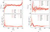 |
Fig. C.3. Complementary data to Fig. 9. (a) Top: Radial component of the gamma effect γr as a function of Rosh (given in the legend), averaged over colatitude θ. Bottom: Radial component of meridional circulation near the equator (colatitude of θ = 80°, see the dotted lines in Fig. 8h,l). Solid lines indicate runs where the dipole is stable, and dashed lines to the runs where dipole collapsed. Runs with g ∝ r, Ra = 8 × 10⁶, ξ = 0.2. (b) The same but for g ∝ 1/r2, Ra = 1 × 10⁶, ξ = 0.2. Subscripts ϕ and θ denote azimuthal and latitudinal average, respectively. Same units as in Fig. 3(c-e). |
Appendix D: Evolution of rotation properties in 1D models
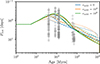 |
Fig. D.1. Surface rotation period as function of age for models with 0.55M⊙ (solid lines), 0.7M⊙ (dashed lines) and 1M⊙ (doted lines). The color corresponds to various values of additional viscosity (in unit of cm2 s−1). For all models, the initial conditions include a disk with a lifetime of 5 Myrs and a period of rotation of 10 days. Gray plus symbols correspond to the measured rotation period of stars in open clusters NGC2547 (40 Myrs), aPersei (85 Myrs), the Pleiades (125 Myrs), Praesepe (600 Myrs) and the Hyades (700 Myrs). Estimated properties taken from Wright et al. (2011). |
All Tables
Main physical ingredients used in the Cesam2k20 models computed for this work.
All Figures
|
Fig. 1. Evolution of a 0.55 M⊙ model. Top: Kippenhahn diagram. Radius of interfaces in solar unit as a function of the model’s age. Convective zones (resp. radiative zones) are represented as dark (resp. light) gray areas. Middle: Aspect ratio (left axis) and density contrast (right axis). The inner radius, ri, is the bottom radius of the convective envelope, while the outer radius, ro, is 90% of the photospheric radius. Bottom: Kelvin-Helmholtz (blue) and convection (green) timescales and surface rotation period (red). The shaded areas correspond to the classical T Tauri phase (CTTS; light green), which coincides in our case with the disk-locking phase and weak T Tauri phase (WTTS; green). |
| In the text | |
|
Fig. 2. Normalized gravitational acceleration g/gmax (top panel) and normalized angular velocity Ω/Ωsurf (bottom panel) as a function of the radius. These profiles are shown at the beginning (blue), middle (orange), and end (green) of the WTTS phase. Same model as in Fig. 1. |
| In the text | |
|
Fig. 3. Patterns of convection with different gravity profiles. (a) Normalized gravity profiles from stellar evolution code Cesam2k20 for a star of 0.8 M⊙ at an early stage of stellar evolution (1 Myr, in light gray) and at the MS (4.9 ⋅ 103 Myrs, dark gray). Example of imposed gravity profiles in DNS: g ∝ 1/r2 for radii ratio ξ = 0.35 (in red), g ∝ r and ξ = 0.2 (in dashed light blue) and a typical profile from Cesam2k20 with ξ = 0.35 (in magenta, see Eq. (3) for detail). (b) Local convective Rossby number, normalized with its maximum, as a function of r/ro for the runs gr2_2, gr_1, and gc_2, associated with the gravity profiles of panel (a) (same color code), and for the run gr2_3, with g ∝ 1/r2 and ξ = 0.2 (in dashed red). Details of the runs are presented in Table B.1. (c) Equatorial cut of instantaneous radial velocity for g ∝ 1/r2, ξ = 0.35 (run gr2_2). (d) Same as (c) but for g ∝ r, ξ = 0.2 (run gr_1). (e) Same as (c) but for g ∝ 1/r2, ξ = 0.2 (run gr2_3). Velocities in panels (c-e) were normalized with ν/(ro − ri), i.e., kinematic viscosity, ν, and the thickness of convective zone. |
| In the text | |
|
Fig. 4. Local convective Rossby number as a function of normalized radius, r/ro, for the typical values of Rosh considered in this work. The gravity profile is from Cesam2k20, approximated by Eq. (3). (See run gc_1 in Table B.1 for more details on the parameters.) |
| In the text | |
|
Fig. 5. Butterfly diagrams of the axisymmetric radial magnetic field component, ⟨Br⟩ϕ, together with the dipolarity. The term Ωst corresponds to the rotation time and follows the uniform rotation of a meridional plane. (a) Stable dipole for g ∝ 1/r2, Ra = 5 × 10⁶, ξ = 0.35, Rosh = 0.005. (b) Equatorially propagating dipolar waves for the same parameters, except for Rosh = 0.02. (c) Aperiodic dynamos for g ∝ 1/r2, Ra = 5 × 10⁵, ξ = 0.1, Rosh = 0.015. (d) Steady quadrupolar dynamos for g ∝ r, Ra = 1.6 × 10⁷, ξ = 0.2, Rosh = 0.3. The magnetic field was normalized with (ρoμ0λiΩs1/2), where ρo is the density at the outer boundary, λi is magnetic diffusivity at the inner boundary, and μ0 is the free space permeability. |
| In the text | |
|
Fig. 6. Ratio of the local radial shear to the local convective Rossby number as a function of latitude (in degree) at the midgap, r/ro = 0.5, for varying Rosh. Solid lines denote stable dipolar states, with magnetic topology as depicted in Fig. 5a, and dashed lines denote collapsed dipoles as those depicted in Fig. 5b. |
| In the text | |
|
Fig. 7. Integral properties of the dynamo with increase of differential rotation. (a) Time-averaged dipolarity parameter as a function of the ratio between shear and convective Rossby numbers for Pm = 4 and three different gravity profiles: g(r) from CESAM in Eq. (3) in magenta, g ∝ 1/r2 in red, and g ∝ r in blue. The lines represent the following: solid lines, ξ = 0.35; dashed, ξ = 0.2; and dotted, ξ = 0.1. More (less) transparent lines correspond to the runs with a lower (higher) Ra number, for a fixed gravity profile and radius ratio (see Table B.1). The shapes represent the following: filled circles, stable dipoles (Fig. 5a); empty circles, reversing dipoles; diamonds, dipolar-quadrupolar waves (Fig. 5b); crosses, mixed dipolar and multipolar solutions without coherent temporal dynamics (Fig. 5c); and squares, equatorially symmetric solutions (Fig. 5d). (b) Same as in panel (a) but for g ∝ 1/r2 only and varying radius ratio. Light color, Pm = 4; dark color Pm = 6. Line styles and symbols as in panel (a). (c) Ratio of rms of axisymmetric toroidal and poloidal magnetic components Btaxi and Btaxi. Runs, lines, and symbols are the same as in panel (a). (d) Estimated critical collapse value of Rosh/Roconvℓ from all curves in panels (a) and (b), as a function of Pm and radius ratio ξ (stars) and the corresponding exponential fits (lines, Eq. 7). |
| In the text | |
|
Fig. 8. Meridional distribution of the relevant dynamo properties. From left to right, the panels show the azimuthally averaged snapshots of the radial magnetic field component ⟨Br⟩; flow helicity H = ⟨U ⋅ ∇ × U⟩; the r component of the γ effect, which is axisymmetric by definition (6); and meridional circulation ⟨Ur⟩. All runs are without imposed differential rotation at the bottom of the convective zone (Rosh = 0). Top row (panels a–d): g ∝ 1/r2, Ra = 5 × 10⁶, and ξ = 0.35. Middle row (panels e–h): g ∝ r, and Ra = 8 × 10⁶, ξ = 0.2. Bottom row (panels i-l): g ∝ 1/r2, Ra = 1 × 10⁶, and ξ = 0.2. The dotted line corresponds to the considered latitude in the bottom panels of Figs. 9 and C.3. The γ effect and ⟨Ur⟩ are normalized using viscous units of the code (see Fig. 3); helicity is thus normalized by ν2/d3. Magnetic field units are the same as in Fig. 5. |
| In the text | |
|
Fig. 9. Competition of the gamma effect with meridional circulation. Top: Radial component of the gamma effect γr as a function of Rosh (legend) averaged over colatitude, θ. Bottom: Radial component of meridional circulation near the equator (colatitude of θ = 80°, see Fig. 8d). Solid lines indicate that the dipole is stable; dashed lines show that the dipole has collapsed. The data are from the runs with g ∝ 1/r2, Ra = 5 × 10⁶, and ξ = 0.35 (gr2_2 in Table B.1). Subscripts ϕ and θ denote azimuthal and latitudinal average, respectively. The units are the same as in Figs. 3(c–e). |
| In the text | |
|
Fig. 10. Data for time-averaged dipolarity from all runs of this paper as a function of compensated shear Rossby number (i.e., Rosh/Roconvℓ) and normalized by its critical value given in Eq. (7). All transitions from dipolar to oscillatory branches collapse on each other. The branch that does not follow the trend is the special case of g ∝ r and the high Ra values (run gr_2 in Table B.1, see Fig. 5d and discussion in Sect. 4.3). Colors, symbols, and lines are the same as in Fig. 7. |
| In the text | |
|
Fig. 11. Evolution with stellar age of the ratios Rosh, Hp/Roconv, mid (solid lines) or Rosh, glob/Roconv, mid (dashed lines). The color corresponds to the additional viscosity considered for the angular momentum transport. The dotted black line corresponds to the threshold defined in Eq. (7) for Pm = 4, with a minimum value of 0.1. Each panel corresponds to a given evolutionary track, whose initial parameters are given in each plot. |
| In the text | |
|
Fig. 12. Mass-period (surface) distribution of some models randomly chosen in the grids described in Sect. 5.3. The criterion considered for the stability of the dipole is the ratio Rosh, Hp/Roconv, mid with the threshold expressed in Eq. (7). Circles and stars are respectively PMS and MS models. Red (resp. green) markers are models that lost (resp. kept) their dipole between their formation and their present age. Each panel corresponds to a grid with a given additional turbulent viscosity, νadd. |
| In the text | |
|
Fig. C.1. Distribution of dimensionless local radial shear Roshl as given in Eq. (5) for the run with g ∼ 1/r2, Ra = 5 × 10⁶, ξ = 0.35. Dotted line denotes the location of tangent cylinder. (a) Rosh = 0, without imposed differential rotation at the bottom of the convection zone. This case corresponds to naturally developing deviation from solid-body rotation with Ωs, due to the turbulent and magnetic stresses of the convective dynamo. (b) Rosh = 0.0125, before collapse; (c) Rosh = 0.015, at the dipole collapse; (d) Rosh = 0.02, after the collapse. |
| In the text | |
|
Fig. C.2. Latitudinal component of the γ effect, γt, corresponding to the three runs in Fig. 8. (a) g ∼ /r2, Ra = 5 × 10⁶, ξ = 0.35; (b) g ∼ r, Ra = 8 × 10⁶, ξ = 0.2; (c) g ∼ 1/r2, Ra = 1 × 10⁶, ξ = 0.2. The overall symmetry of γ effect remains the same, despite the small-scale noise. Same units as in Fig. 3(c-e). |
| In the text | |
|
Fig. C.3. Complementary data to Fig. 9. (a) Top: Radial component of the gamma effect γr as a function of Rosh (given in the legend), averaged over colatitude θ. Bottom: Radial component of meridional circulation near the equator (colatitude of θ = 80°, see the dotted lines in Fig. 8h,l). Solid lines indicate runs where the dipole is stable, and dashed lines to the runs where dipole collapsed. Runs with g ∝ r, Ra = 8 × 10⁶, ξ = 0.2. (b) The same but for g ∝ 1/r2, Ra = 1 × 10⁶, ξ = 0.2. Subscripts ϕ and θ denote azimuthal and latitudinal average, respectively. Same units as in Fig. 3(c-e). |
| In the text | |
|
Fig. D.1. Surface rotation period as function of age for models with 0.55M⊙ (solid lines), 0.7M⊙ (dashed lines) and 1M⊙ (doted lines). The color corresponds to various values of additional viscosity (in unit of cm2 s−1). For all models, the initial conditions include a disk with a lifetime of 5 Myrs and a period of rotation of 10 days. Gray plus symbols correspond to the measured rotation period of stars in open clusters NGC2547 (40 Myrs), aPersei (85 Myrs), the Pleiades (125 Myrs), Praesepe (600 Myrs) and the Hyades (700 Myrs). Estimated properties taken from Wright et al. (2011). |
| In the text | |
Current usage metrics show cumulative count of Article Views (full-text article views including HTML views, PDF and ePub downloads, according to the available data) and Abstracts Views on Vision4Press platform.
Data correspond to usage on the plateform after 2015. The current usage metrics is available 48-96 hours after online publication and is updated daily on week days.
Initial download of the metrics may take a while.