| Issue |
A&A
Volume 708, April 2026
|
|
|---|---|---|
| Article Number | A235 | |
| Number of page(s) | 20 | |
| Section | Extragalactic astronomy | |
| DOI | https://doi.org/10.1051/0004-6361/202557118 | |
| Published online | 08 April 2026 | |
Impact of stochastic star formation histories and dust information on selecting quiescent galaxies with JWST photometry
1
National Centre for Nuclear Research, Pasteura 7, 093 Warsaw, Poland
2
SISSA, Via Bonomea 265, 34136 Trieste, Italy
3
Department of Physics & Astronomy, University of British Columbia, 6224 Agricultural Road, Vancouver BC V6T 1Z1, Canada
4
Department of Astronomy and Physics, Saint Mary’s University, 923 Robie Street, Halifax NS B3H 3C3, Canada
5
Canada Research Chair in Astronomy and Astrophysics (Tier II), Canada
6
Max-Planck-Institut für Radioastronomie, Auf dem Hügel 69, 53121 Bonn, Germany
7
INAF, OAPD, Vicolo dell’Osservatorio, 5, 35122 Padova, Italy
8
Dipartimento di Fisica e Astronomia, Universitá di Bologna, Via Gobetti 93/2, 40129 Bologna, Italy
9
Department of Astronomy, The University of Washington, Seattle, WA, USA
10
Instituto de Astrofísica de Canarias, Vía Láctea S/N, E-38205 La Laguna, Spain
11
Departamento de Astrofísica, Universidad de La Laguna, E-38206 La Laguna, Spain
12
Kavli Institute for Cosmology Cambridge, Madingley Road, Cambridge CB3 0HA, UK
13
Institute of Astronomy, University of Cambridge, Madingley Road, Cambridge CB3 0HA, UK
14
Zentrum für Astronomie der Universität Heidelberg, Astronomisches Rechen-Institut Mönchhofstr, 12-14 69120 Heidelberg, Germany
15
Astronomical Observatory Institute, Faculty of Physics, Adam Mickiewicz University, ul. Słoneczna 36, 60-286 Poznań, Poland
16
Institute of Astronomy, Faculty of Physics, Astronomy and Informatics, Nicolaus Copernicus University, Grudzidzka 5, 87-100 Toruń, Poland
17
Astronomical Observatory of the Faculty of Physics, Astronomy and Applied Computer Science, Jagiellonian University, ul. Orla 171, 30-244 Kraków, Poland
★ Corresponding author: This email address is being protected from spambots. You need JavaScript enabled to view it.
Received:
5
September
2025
Accepted:
25
February
2026
Abstract
Context. The James Webb Space Telescope (JWST) enables the identification of quiescent galaxies out to early epochs, offering a transformative view of their evolution. However, the photometric selection of quiescent galaxy candidates (QGCs) and the derivation of their key physical quantities, such as stellar masses (M★) and dust attenuation, remain highly sensitive to the assumed star formation histories (SFHs), where dust–age degeneracies and modelling choices continue to stand as a major source of uncertainty.
Aims. We aim to quantify how the inclusion of JWST/MIRI data and different SFH models impacts the selection and characterisation of QGCs. We test the robustness of the physical properties inferred from the spectral energy distribution (SED) fitting, such as M★, age, star formation rate (SFR), and dust attenuation (AV). We study how these parameters impact the quiescence criteria of the galaxies across cosmic time.
Methods. We performed SED fittings for ∼13 000 galaxies at z ≤ 6 from the CEERS/MIRI fields with a ≤20 optical to mid-infrared broadband coverage. We implemented three SFH prescriptions: a flexible delayed model, a non-parametric model, and an extended regulator model. For each SFH, we compared the results obtained with and without MIRI photometry and dust emission models. We evaluated the impact of these configurations on both the number of QGCs, selected on the basis of their rest-frame UVJ colours, specific SFR, and main-sequence offset, as well as on their key physical properties, such as M★, AV, and stellar ages.
Results. The number of selected QGCs varied significantly, with the SFH ranging from 70 to 100 out of a mass-complete sample of ∼5000 galaxies, depending on the model. This number increased to 103–180 when MIRI data were included, driven by improved constraints on both dust attenuation and M★. We found a strong correlation between AV and M★ of QGCs at z ≤ 2.5, with massive galaxies (M★ ∼ 1011 M⊙) shown to be ∼ 1.5 − 4 times more attenuated than low-mass galaxies (M★ ∼ 109 M⊙). Regardless of the SFH, ∼13% of QGCs exhibit significant attenuation (AV > 0.5) in support of recent JWST results on dust-rich quiescent galaxy candidates.
Key words: galaxies: evolution / galaxies: ISM
© The Authors 2026
 Open Access article, published by EDP Sciences, under the terms of the Creative Commons Attribution License (https://creativecommons.org/licenses/by/4.0), which permits unrestricted use, distribution, and reproduction in any medium, provided the original work is properly cited.
This article is published in open access under the Subscribe to Open model. This email address is being protected from spambots. You need JavaScript enabled to view it. to support open access publication.
1. Introduction
Quiescent galaxies (QGs), often termed ‘evolved’ or ‘passive’, are characterised by minimal star formation or none at all (Strateva et al. 2001; Willmer et al. 2006; Franzetti et al. 2007) and they lie below the star-forming main sequence (MS; e.g. Speagle et al. 2014; Schreiber et al. 2015; Wang et al. 2022; Popesso et al. 2023; Koprowski et al. 2024; Mérida et al. 2026; Simmonds et al. 2025). The physical mechanisms driving their quenching remain one of the most pressing puzzles in galaxy evolution (Faber et al. 2007; Kriek et al. 2008; Feldmann & Mayer 2015; Man & Belli 2018; Zheng et al. 2022; Akhshik et al. 2023), particularly with the discovery of massive QGs out to z ∼ 5 − 7 (Glazebrook et al. 2017; Valentino et al. 2020; Carnall et al. 2023b; Weibel et al. 2025), which requires rapid quenching processes in approximately the first gigayear of cosmic history. Key questions remain regarding the interplay between quenching and the interstellar medium (ISM), especially for dust, as well as the extent to which broadband photometry alone can be used to constrain quenching timescales and the subsequent evolutionary pathways of QGs.
The advent of the James Webb Space Telescope (JWST) enables the identification of high-z QGs up to z ∼ 7 (e.g. Valentino et al. 2023; Looser et al. 2024; Weibel et al. 2025), as well as QGs of lower stellar masses (M★ < 109 M⊙; Popesso et al. 2023; Mérida et al. 2026). The near- and mid-infrared (NIR-MIR) coverage of the JWST now makes it possible to investigate the age and dust-related parameters, which have long been difficult to disentangle due to the well-known degeneracy of the dust-age-metallicity (Conroy 2013; Santini et al. 2015). Inspecting this link has become an urgent topic, as recent studies have revealed QGs with highly attenuated profiles (e.g. Setton et al. 2024; Lu et al. 2025; Bevacqua et al. 2025) and/or a dust-enriched ISM (e.g. Gobat et al. 2018; Whitaker et al. 2021; Bezanson et al. 2022; Morishita et al. 2022; Donevski et al. 2023; Lee et al. 2024; Lorenzon et al. 2025b). These reports cover a wide range of cosmic epochs (0.4 ≲ z ≲ 4), even though such systems are expected to be dust-poor at the time of observation.
Such discoveries force us to revisit our understanding of QG selection and the derivation of physical parameters from optical and NIR photometry alone. The identification of QGs has been done in different ways throughout the last decades, but mainly focussing on rest-frame colour-colour diagrams (e.g. Arnouts et al. 2013). Such diagnostics allow us to break the degeneracy between dust reddening and stellar population ageing. They are especially powerful in selecting QG candidates (QGCs) from wide-field surveys, for which few photometric bands might be available. The colour-colour diagrams are built with three rest-frame bands: one in the near-ultraviolet to optical, the second in optical range, and the final in the NIR, so as to separate the population of QGs from dusty star-forming galaxies (SFGs). Among many combinations, the U − V versus V − J (hereafter, UVJ) diagram has been extensively tested for selection of QGs across all redshifts (Wuyts et al. 2007; Williams et al. 2009; Krywult et al. 2017; Fang et al. 2018; Akins et al. 2022), given its correlations with the specific star formation rate (sSFR; Williams et al. 2010; Patel et al. 2011; Martis et al. 2019), dust attenuation (Price et al. 2014; Nagaraj et al. 2022; Gebek et al. 2025)), and stellar ages (Whitaker et al. 2013; Belli et al. 2019). However, the UVJ selection is known to be less reliable at z ≳ 3, where the J band cannot be well sampled without rest-frame MIR data. This challenge has motivated the development of new colour selection techniques designed for higher redshifts (Antwi-Danso et al. 2023; Gould et al. 2023; Long et al. 2024; Baker et al. 2025; Merlin et al. 2025).
Other commonly used methods are centred on MS offsets and spectral tracers. Spectral identification is the only reliable way to confirm the quiescent nature of a QGC, as it confirms the absence of ongoing star formation. In particular, the Balmer break is a powerful indicator of the stellar population age, as it strongly correlates with the fraction of old versus young stars (Balogh et al. 1999; Kauffmann et al. 2003; Haines et al. 2017). More precisely, absorption lines as Ca II and Hδ characterise the old stellar population that completely breaks the age-dust degeneracy (Bruzual 1983; Siudek et al. 2017). Emission lines such as [O II] and Hα are instead used as tracers for very recent star formation (Kennicutt 1992; Villa-Vélez et al. 2021). Thus, the spectra encode direct information about stellar populations within galaxies and star formation histories (SFHs; Mathis et al. 2006; Iyer et al. 2020; Iglesias-Navarro et al. 2024). However, depending on the sample size and observing facilities, spectroscopy often requires long observing times and careful planning. In contrast, colour-colour diagrams, which can be obtained by fitting the spectral energy distribution (SED), sketch the dependence between age, dust attenuation and sSFR, while even offering a way to study quenching pathways (e.g. fast vs slow quenchers; Tacchella et al. 2022). They enable the selection of statistical samples of QGCs and take less time to implement in large areas of the sky with a wide range of redshifts (e.g. Daddi et al. 2005; Arnouts et al. 2007; Williams et al. 2009; Ilbert et al. 2013; Wu et al. 2018).
For years, most of the SED fitting codes modelled SFHs with relatively simple analytical functions that depend on only a few parameters (e.g. Walcher et al. 2011; Boquien et al. 2019). The probe of the parameter space of the so-called parametric SFH is quick, but lacks the flexibility to model more diverse SFHs (e.g. with high burstiness or with a few episodes of rejuvenated star formation). Recent studies introduce a new attempt to model SFHs with stochastic changes (e.g. Ocvirk et al. 2006; Finlator et al. 2007; Leja et al. 2019a; Iyer et al. 2024; Annunziatella et al. 2025; Carvajal-Bohorquez et al. 2025).
The methods proposed in these works overcome the simplicity of parametrised SFH without incurring significant additional computational cost. Furthermore, recent simulation-based studies define stochastic and physically motivated SFH models (e.g. Iyer & Gawiser 2017; Tacchella et al. 2020). The new SFH models finally reach the flexibility needed to catch all changes shaping the evolution of a galaxy, but they have not been tested on QGs. Thus, the discussion about constraining SFHs, especially the quenching related timescales, with photometry-only studies is already ongoing (Smith & Hayward 2015; Aufort et al. 2025).
In this work, we leverage JWST deep-field photometry to identify QGCs up to z ∼ 6 and using SED fittings to characterise their SFHs and key physical properties, such as stellar masses, rest-frame colours, and dust attenuations. To achieve this goal, we implemented and compared the non-parametric (Leja et al. 2019a) and extended regulator (Tacchella et al. 2020) SFH models within Code Investigating GALaxy Emission (CIGALE; Boquien et al. 2019), testing their impact on derived galaxy properties. We combined JWST MIR data with stochastic SFH to alleviate any age and dust degeneracies. We systematically evaluated how SFH choices, selection criteria, and the inclusion of MIR observations affect the physical and statistical properties of QGCs. Finally, we study the quenching related timescales and their relation to the physical properties of QGCs within a purely photometric framework.
The paper is organised as follows. In Sect. 2 we describe the data sets and sample selection used in this study. Section 3 offers a brief discussion of the adopted SFHs and our implementation of two new CIGALE modules based on stochastic SFHs, as well as our SED-fitting procedure. In Sect. 4 we present and discuss the results: we first compare how different SFH models affect the statistics of the selected QGCs and then examine how their rest-frame UVJ colours and quenching timescales relate to key physical properties such as M★ and AV. In Sect. 5 we summarise our findings and conclude the study. Throughout the paper, we assume the Λ cold dark matter cosmological model with H0 = 70 kms−1 Mpc−1, Ωm = 0.3, and ΩΛ = 0.7, along with the the Chabrier (2003) initial mass function (IMF). The conversion from other IMFs was performed using multiplicative factors from Madau & Dickinson (2014).
2. Data
We used the data collected from the Cosmic Evolution Early Release Science Survey (CEERS; proposal No. 1345, P.I. Finkelstein; Finkelstein et al. 2022). CEERS covers an area of ≃94.6 arcmin2, previously observed for the 3D Hubble Space Telescope (HST) survey of the All-Wavelength Extended Groth Strip International field (AEGIS; Brammer et al. 2012). The CEERS programme makes use of both JWST imaging instruments, the Near-InfraRed Camera (NIRCam; Beichman et al. 2012) and the Mid-Infrared Instrument (MIRI; Bouchet et al. 2015; Rieke et al. 2015), with a total area covered with MIRI observations reaching ∼28.28 arcmin2. The abundance of MIR coverage in both the area and the number of photometric bands makes CEERS the optimal testing ground for stellar and dust properties of QGCs in a statistical manner, as no other field provides a similar advantage in the study of QGCs evolution.
2.1. HST–JWST/NIRCam photometry
To build our parent catalogue, we used seven NIRCam filters sampled to a pixel size of 0.03 arcsec, out of which six broadband (F115W, F150W, F200W, F277W, F356W, and F444W), one medium-band (F410W), and seven broadband MIRI filters sampled to pixel size of 0.09 arcsec (F560W, F770W, F1000W, F1280W, F1500W, F1800W, and F2100W). We complemented JWST data with six HST broadband filters sampled to a pixel size of 0.03 arcsec (F606W, F814W, F105W, F125W, F140W, and F160W; Stefanon et al. 2017). By combining JWST with HST data, we obtained the wealthy optical to MIR coverage spanning 20 bands. We adopted the HST and JWST NIRCam fluxes from the ASTRODEEP-JWST catalogue (Merlin et al. 2024), which complement NIRCam observations with archival HST observations. The catalogue consists of 82 547 sources and its our parent sample. We took advantage of the homogeneous reduction and flux extraction for both NIRCam and HST observations within the catalogue. Additionally, to keep our sample consistent, we used photometric redshifts calculated by Merlin et al. (2024)1.
For a detailed description of flux extraction and analysis, we refer to Merlin et al. (2024). In short, after re-projecting all the images (NIRCam and HST) to the same pixel grid, the F356W and F444W images were stacked and used as a detection image. SExtractor (Bertin & Arnouts 1996) was used for the detection and flux derivation. The errors were estimated through root mean square (RMS) maps. Comparison with spectroscopic redshifts (zspec) shows that only ∼6% of the sample has a redshift mismatch greater than 0.15 (see Fig. 12 in Merlin et al. 2024).
The catalogue is 90% complete at ∼29.04 mag in stacked F356W and F444W filters (Fig. A.1; see also Fig. 4 in Merlin et al. 2024). According to our analysis (Appendix A), it translates to 90% completeness at M* ∼ 107.9 M⊙ at z = 6 for the entire catalogue. The completeness for the QG-only sample reaches a similar depth, while for SFGs only, we estimated 90% completeness at M* ∼ 107.6 M⊙ for the same redshift.
2.2. MIRI photometry
We performed optimised extractions of MIRI fluxes across all available MIRI bands. The detailed description of MIRI flux estimates, their associated errors, and inferred upper limits, can be found in Appendix B. In brief, we extract total fluxes from MIRI sources in each of the pointings using SExtractor. We used the MIRI mosaics version 0.6 data release (Yang et al. 2023b), which is characterised by corrected astrometry based on the HST reference. We followed Yang et al. (2023b) and use the MAG_AUTO parameter for flux measurements. We cross-matched the NIRCam/HST catalogue from Merlin et al. (2024) with our MIRI fluxes within a 0.5-arcsec radius. In our catalogue and further SED fitting, we put a 5σ upper limit for MIRI fluxes when no direct detection (no source in crossmatch radius or signal to noise < 3) is found. We used 5σ (instead of 3σ) since our analysis of upper limits was performed for point-like sources and the galaxies were spatially resolved. The upper limits values vary, depending on the band and the MIRI pointing, from the deepest 26.75 mag for F770W pointing 3, to 23.64 mag for F2100W pointing 1 (see the full list of 5σ AB upper limits in Table B.2).
2.3. Final sample
Our aim in this study is to understand how the inclusion of MIR points (crucial to assess age-dust degeneracy), combined with the SFH model choice, affects the selected QGCs and their physical properties. For this reason, we restrict the parent CEERS catalogue to include only sources within the CEERS/MIRI footprint covering ∼28.28 arcmin2.
This limitation results in a sample in which all our sources have been observed in at least one MIRI band. Since the MIRI footprints of different filters are not equal (see the coverage of pointings in Table B.2), the number of filters covering a single source can vary from one to six. This choice restricts us to 12 939 galaxies for which 1 939 have direct MIRI detection above 3σ. The remaining 11 000 have at least one MIRI upper limit2. We show the redshift distribution of these galaxies in Fig. A.1.
Finally, throughout this work, we focussed solely on a mass-complete sample. Thus, we chose to study only galaxies with stellar masses above the 90% completeness limit, M★ ≥ 108 M⊙, in all three SED fitting MIRI runs (see Sect. 3.2). Our final sample consists of 5021 galaxies at 0.1 ≲ z ≲ 6 out of which 1574 have at least one detection in the MIRI bands3. We have: 572, 832, 41, 117, 3, and 9 sources observed in 1, 2, 3, 4, 5, and 6 MIRI bands in final sample, respectively.
We are aware that the active galactic nucleus (AGN) dust emission can contribute to MIRI photometry (e.g. Yang et al. 2023a). Therefore, we conducted a test to evaluate its impact on our results. We cross-matched the final sample with the 42 AGN candidates identified in the CEERS/MIRI observations (pointings 1, 2, 5, and 8), as described in Chien et al. (2024), resulting in 24 direct counterparts. The AGN contamination in our QGC sample (see Sect. 4.3) is approximately 4%. Furthermore, none of the AGN contaminants in our QGCs exceed a V-band attenuation of 0.5 mag. Nevertheless, we removed these known contaminant sources from any QGCs sample in the following analysis.
3. SED modelling
We used CIGALE (version 2022.01; Boquien et al. 2019), as it is optimised for broadband photometry, to model and fit the SED of observed galaxies. CIGALE uses energy balance conservation between the dust-absorbed stellar emission and its re-emission in the IR. It goes over a grid of models, with the parameter values set by the user, and identifies the best fit by minimising chi square (χ2). We took advantage of the modularity of CIGALE and implement stochastic SFHs within the framework (see Appendices C.1 and C.2).
3.1. Star formation histories
With respect to SFHs in CIGALE, there are two main approaches that are typically implemented. The first one is straightforward, using previously prepared SFH (i.e. templates or directly from simulations) as input to test what SED will end up being produced with a given SFH. The second is built on parametric models. Parametric SFHs assume that star formation in a galaxy is a continuous process, which can be described by a few parameters such as the age and the e-folding time of the main stellar population. For a detailed description of all available SFH parameterisations, we refer to Boquien et al. (2019).
For the purpose of this study, we implemented the diverse stochastic SFHs within CIGALE, namely, non-parametric (Leja et al. 2019a; Carnall et al. 2019) and extended regulator (hereafter, regulator; Tacchella et al. 2020). The description of the implementation and technical details, as well as the original method can be found in Appendix C. We also share the implementation in the form of a public GitHub repository4. Throughout the study, we provide detailed comparisons of results achieved with three SFH models: parametric flexible delayed + burst-quenching model (delayedBQ hereafter), non-parametric, and regulator. The visual comparison of specific SFH (sSFH) models prepared with new modules used in this work is shown in the bottom panel of Fig. 1.
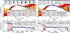 |
Fig. 1. Exemplary QGCs from our final sample: Massive system on the left and a less massive one on the right. Top: CIGALE SEDs. Solid and dashed black lines show the best–fit SEDs for the same galaxy using the regulator SFH with and without JWST/MIRI photometry for the MIRI and no–MIRI runs, respectively. Blue circles are detections; triangles are 3σ upper limits. JWST cutouts are displayed above each SED. Shaded envelopes indicate the range of K–band–normalised SEDs for QGCs binned by median AV; the legend lists the median AV values and number of objects in each bin. Bottom: sSFHs for the same QGC from the MIRI run. The solid dark blue, dashed violet, and dash-dotted light blue lines correspond to the regulator, non-parametric, and delayedBQ models, respectively. The thick and thin dark-blue lines show the difference between MIRI and no-MIRI runs. The dotted black line marks the quiescent threshold and the dashed black line the star-forming threshold (following Pacifici et al. 2016). Arrows mark the quantities used in this work for the regulator model: the quenching time, Tq, the quenching moment, τq, the cosmic time at the observation redshift, τ(zo), and the time since quenching, ΔT ≡ τ(zo)−τq. |
In the non-parametric SFH model, the star formation rate (SFR) changes randomly between defined time steps. The changes follow the Student-t distribution. We followed the implementation described by Leja et al. (2019a) with prior continuity. This approach results in reduced burstiness, namely, fewer rapid changes in the SFR over time. In our implementation, we allowed for five parameters (an exemplary set of parameters can be found in Table C.1) in this module.
For the regulator model, we followed the approach described in Tacchella et al. (2020) and Iyer et al. (2024). The regulator SFH model is based on the control of the SFR by the assigned gas mass reservoir. The stochastic nature of the SFR is a result of (1) gas inflow and outflow rates; (2) gas cycling in equilibrium between atomic and molecular states; and (3) the formation, lifetime, and disruption of giant molecular clouds (GMCs). In our implementation, we allowed for eight parameters in the regulator model (an exemplary set of parameters can be found in Table C.1).
The delayedBQ mode (Ciesla et al. 2016, 2021) is a flexible extension of the classical delayed-τ model. By adding an instantaneous quench or burst, the delayedBQ model is flexible for better sensitivity to SFR within recently quenched galaxies. The delayedBQ model takes the following form,
 (1)
(1)
where t is the time, τmain is the e-folding time, tflex is the time at which star formation is affected by instantaneous change, and RSFR is the ratio between SFR(t > tflex) and SFR(t = tflex), expressed as
 (2)
(2)
3.2. SED fitting runs and parameter space
To study the influence of the SFH model on the estimated physical properties, such as M★, SFR, or V-band attenuation (AV), we performed three runs: (1) with the parametric delayedBQ model; (2) with the non-parametric model; and (3) with the regulator model. We kept all parameters that were not related to the SFH the same between runs. The only ones that were adjusted were the SFH variables, which are module-dependent, and the stellar population ages (depending on redshift). We summarise the main methods and parameters used for our models in the following, with explicit values detailed in Appendix C.3.
For the non-parametric module, we used nLevels = 8, since it was shown through testing that robust results can be achieved with 4≤ nLevels ≤ 14 (Leja et al. 2019a; Tacchella et al. 2020; Lower et al. 2020). The lastBin parameter was set to 30 Myr following Leja et al. (2019a) and Ciesla et al. (2023). We made a total of five iterations of each run with both stochastic SFH modules to test the stability of the results (see Appendix D). In each iteration, we set nModels to 200. In total, we generated 1000 random sampled SFH models, with each of them tested in CIGALE. Thus, we were able to obtain not only the best model (found by the least reduced χ2), but also a group of five iterations of the best models per stochastic SFH. In other words, each galaxy has five independent solutions within the same stochastic SFH model framework. We took advantage of this by checking the stability of the solution. Whenever we used all five solutions, we mention it explicitly in the text. According to our tests, splitting the CIGALE run into five smaller runs to sample more SFH models does not influence the results. More details can be found in Appendix D.
For the regulator module, we set nLevels to 300. The number of time-steps in the regulator model is not limited as much as in non-parametric, since the SFR changes are physically motivated. Although this number is arbitrary, it results in a time resolution that is always better than ∼45 Myr per step (depending on the formation redshift and the observation redshift). This is enough to distinguish, for example, fast quenchers (quenching time < 100 Myr) from slow quenchers (Belli et al. 2019; Tacchella et al. 2022). The nModels parameter, similarly to the non-parametric run, is tested in five iterations by 200 each, in total 1000 SFH models. The parameters regulating variability and time scales, sigmaReg, tauEq, tauFlow, sigmaDyn, and tauDyn, were set at 1, 1300, 125, 0.07, and 35, respectively. These values are between the Milky Way analogue and the cosmic noon galaxy from Iyer et al. (2024). Since we expect a diverse galaxy population in our sample, we decided to make it a compromise, as checking all combinations is beyond our computational capabilities and outside the scope of this study.
We are aware of high burstiness reported in high-z (z > 2.5) and/or low-M★ (logM★/M⊙ < 109) galaxies (e.g. Cole et al. 2025; Mintz et al. 2026). To rule out its importance for our analysis, we conducted additional tests for a lower number of galaxies, with sigmaReg = 1, 1.5, 2, 3. We report that the results (M★, AV, SFR, and age) found with different values of sigmaReg are consistent within the uncertainties reported by CIGALE. Thus, we expected this parameter to have a low-influence in the analysis, described below.
In all runs, we assumed Bruzual & Charlot (2003) single stellar population models with the IMF given by Chabrier (2003). We used the Charlot & Fall (2000) attenuation module, as our main interest here is to study how the inclusion of MIRI data reflects the SFH output. This module assumes two separate attenuation curves for young and old stellar populations. Finally, we used the dust emission model described in Draine et al. (2014).
Since our sample covers a broad redshift range (0 < z < 6), we split it into five sub-samples with lower redshift coverage. The main purpose is to keep the computation relatively easy, with as little change in input parameters as possible. The number of galaxies within each sub-sample, redshift ranges of the sub-samples, and their influence on the input parameters are shown in the first part of Table C.1.
To test the influence of the dust component and MIR observations on the results, we performed a second set of CIGALE runs using the same final sample, but without observed MIRI data (fluxes and/or upper limits). Since we have restricted our data to the NIR, we also disabled the dust emission model to speed up the calculations. All other parameters remained the same. Henceforth, the main runs with inclusion of MIRI data and dust emission module are referred to as ‘MIRI runs’. The second set, with no MIRI data and dust emission module included, is referred to as ‘no-MIRI runs’. The exemplary SEDs for both MIRI and no-MIRI runs are presented in the upper panel of Fig. 1. Throughout the analysis, we utilised the Bayesian values of each property estimated by CIGALE (through an internal Bayesian procedure), unless explicitly stated otherwise. The M★–z distribution of the final sample for the regulator SFH model is presented in the upper panel of Fig. 2. Furthermore, the redshift and M★ histograms are presented in Fig. A.1. The photo-z errors are not propagated.
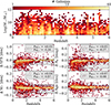 |
Fig. 2. Top: Distribution of the M★ in function of redshift of the final sample from the regulator MIRI run. Bottom: Distributions of differences in the main physical properties (SFR in M⊙/yr and the M★ in M⊙, AV in mag, age in Myr) between the MIRI and no-MIRI runs. The hatched region shows the 90th percentiles of the distributions (P90) in both directions. |
4. Results and discussion
In this section we investigate and discuss the influence of SFH, MIRI data, and selection criteria on the number of QGCs selected. This is followed by a comprehensive analysis of capabilities to constrain the SFHs with the photometry-only SED fitting. Finally, we study the inferred quenching-related properties and dust attenuation evolution after quenching.
We focussed our study on four fundamental global physical properties: M★, the SFR (averaged over 10 Myr), AV, and the age (look-back time of formation age, i.e. the time since the onset of star formation). To quantify the stability of the physical properties, we used the coefficient of variation (CV, relative standard deviation), CV = σ/μ, where σ is the standard deviation (calculated from five iterations) and μ is the value of the physical property such as M★, SFR, or AV of the iteration with the lowest χ2.
As a sanity check, we tested the stability of the results with stochastic SFH within the final sample. Since in each iteration, all the SFH models were different, the best result found by CIGALE will vary, unlike that of the parametric SFH. The resulting scatter in the inferred physical properties, such as M★ or SFR, is quantified in Appendix D. We report a high level of consistency between iterations for both non-parametric and regulator models for M★ (on average, M★ values in each iteration differ by less than 6%), AV (below 8%) and age (below 6%). A similar consistency was found for SFR but only in the regulator model (below 3%). The SFR in the non-parametric can vary up to ∼30%. However, this variation is mainly due to low SFR values, which does not influence the overall selection.
4.1. Influence of MIRI data on inferring physical properties
We further tested how incorporating MIRI data and dust emission models in the SED fitting affects the results, compared to SED fits that exclude both. The comparisons of the distributions from the no-MIRI and MIRI runs, for regulator SFH used as reference model, are presented in Fig. 2.
In general, we find that the inclusion of MIRI measurements has a negligible effect on the derived M* (P90 < 0.09 dex) and ages (P90 < 0.1 dex), which remain consistent in all SFH. This was confirmed for high-mass galaxies (M★ > 1010 M⊙; Wang et al. 2025), but we found a similar accuracy for lower-mass galaxies as well. However, it plays a crucial role in the constraint of SFR and AV. This SFR-AV degeneration is expected when no IR coverage is available (see e.g. Riccio et al. 2021; Małek et al. 2024), since CIGALE uses the energy budget balance. In our case, without MIRI, the SFRs are systematically overestimated up to 0.65 dex (with a median ∼0.1 dex) due to poorer constraints on dust emission, which regulates energy balance. Thus, the QGC samples are more complete in MIRI runs. Similarly, in the absence of MIR coverage, AV exhibits a small but steady asymmetric bias towards higher values, up to 0.25 mag (with a median of ∼0.06 mag).
These results highlight the importance of MIRI to better constrain the IR side of the SED (thus energy balance) and help overcome degeneracies between dust and age in QGs. By including MIR points and dust emission, we were able to put a soft prior on the energy absorbed by dust (i.e. the SFR). However, we must mention that while JWST clearly helps to overcome the degeneracy between dust and age, there is still the degeneracy between metallicity and age that needs to be addressed (e.g. Cheng et al. 2025). This will be explored with spectroscopic data in future work.
It is worth noting that galaxies with at least one MIRI detection from our final sample are generally at a lower z, with a median of z ∼ 1.8, compared to z ∼ 2.4 for the entire final sample. Similarly, these galaxies have higher M★ (median at 109.2 M⊙) compared to the final sample (108.7 M⊙). This is caused by shallower observations with MIRI, compared to NIRCam. The distributions of the other parameters do not vary significantly.
4.2. Impact of SFH modelling on derived physical properties
To understand the biases introduced by the choice of the SFH model in deriving M★, AV, SFR, and age of QGCs, we first studied the influence of SFH on the whole sample. We utilised the MIRI run. In Fig. 3 we compare the physical quantities of the SED runs with different SFH models. We can report a great agreement for all properties apart from SFR with the non-parametric SFH model. The estimations of M★ and age are consistent up to ∼0.15 dex and AV up to ∼0.3 mag between SFH models. The SFR estimated with delayedBQ and regulator models agree up to ∼0.4 dex. The SFR stability between iterations with the use of the non-parametric model is low, especially for negligible SFR values (see Appendix D). The strong underestimation of SFR by the non-parametric model is prominent only in low-SFR galaxies and we can assume an overall consistency up to ∼0.5 dex compared to other SFH models. A similar underestimation of SFR, reaching ∼0.3dex, in low-SFR galaxies (logSFR < 0) has been shown by comparing direct cosmological simulation results with the CIGALE SED fitting of mock observations of the same galaxies (see Fig. 4 from Arango-Toro et al. 2025). Additionally, Annunziatella et al. (2025) showed that the non-parametric model favours a faster mass assembly than parametric models. This may result in earlier quenching (compared to parametric SFHs models), followed by lower values of SFR. The comparison between regulator and non-parametric SFH models correlates well with the results of Wan et al. (2024).
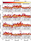 |
Fig. 3. Difference in estimated physical properties of galaxies from the final sample using different SFH models within the MIRI run as a function of redshift. From left to right: DelayedBQ-non-parametric, non-parametric-regulator, and regulator-delayedBQ. From top to bottom: Distribution of difference for: AV in mag, age in Myr, SFR in M⊙/yr, and the M★ in M⊙. The dashed blue line presents the median of distribution. The hatched region shows the 90th percentiles of the distributions (P90) above and below the median value. |
Across the three SFH methods, the dominant source of discrepancy arises from fundamentally different constraints on the accessible individual models. Parametric models such as delayedBQ enforce smooth evolutionary shapes with a single sharp feature such as quenching or burst. The non-parametric approach allows for arbitrary temporal structure and, consequently, reconstructs more complex or discontinuous histories when the data permit. The regulator SFH restricts solutions to be consistent with gas-cycling physics, tying the SFR evolution to inflow, outflow, and efficiency prescriptions. As a result, each method interprets the same observational features through a different optics. These factors lead to systematic mismatches in inferred SFRs (see Fig. 3) and mass-assembly timescales (e.g. Annunziatella et al. 2025).
4.3. Photometric selection of QGCs: Impact of SFH models
In the next step, we tested the effect of the selection criteria on the resulting QGCs sample for each SFH model in both MIRI and no-MIRI CIGALE runs. We tested various popular and empirically defined methods for selecting QG, such as MS (Popesso et al. 2023; Koprowski et al. 2024; Mérida et al. 2026), the criterion based on the sSFR (sSFR ≡ SFR/M*) proposed by Pacifici et al. (2016) and UVJ selection with correction for z > 4 sources (Antwi-Danso et al. 2023). Using more than one definition of QGC can reveal whether the SFH model is more influential than the QGC selection criterion. We report the effect of the selection criteria on the resulting QGCs sample for each SFH model in both MIRI and no-MIRI CIGALE runs. The comparison of the number of QGCs selected with different SFH and criteria is shown in Fig. 4. We find that both choice of SFH and inclusion of MIRI data strongly impact photometric selection of QGCs, but interestingly these effects appear to be independent of each other. We normalised all of our selection criterion to the Chabrier (2003) IMF. Our prime attention in the following analysis would be to the most conservative criterion, which is the one based on the sSFR (see below).
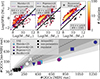 |
Fig. 4. Top: SFR-M★ plane for different redshifts with galaxies from the final sample from the MIRI run with the regulator SFH. The different lines present quiescence selection from the literature: the sSFR criterion in black; Popesso et al. (2023) in dark blue; Koprowski et al. (2024) in violet; and Mérida et al. (2026) in light blue. The grey crosses represent QGCs selected by the sSFR criterion in the regulator MIRI run, which were not recovered in the no-MIRI run. Bottom: Comparison of the QGCs sample size, depending on the selection criterion and SFH model for the MIRI and no-MIRI runs. The colours of the points represent the MSs and are the same as at top panel. The markers represent SFH model: Regulator (triangle); non-parametric (circles); and delayedBQ (squares). The dashed line shows one-to-one relation. With the shaded regions we mark 30%, 60%, and 100% relative distance from the one-to-one relation. |
4.3.1. Main sequence selection
To select QGCs with MS, we applied the same widely used MS offset to all scaling relations: log(SFR/SFRMS) < − 0.6 (e.g. Elbaz et al. 2018; Donevski et al. 2020; Lisiecki et al. 2023), where SFRMS is the SFR predicted by given MS according to the stellar mass and redshift of the galaxy. The visual interpretation of MS based quiescence thresholds are shown at Fig. 4.
The choice of MS, while maintaining the SFH model, influences the number of selected QGCs up to factor of ∼2. This is expected since each MS is defined by the use of different samples, where even a selection of SFGs strongly influences the MS shape (Pearson et al. 2023). We find that the choice of SFH has a greater influence on the number of selected QGCs by up to a factor of ∼3.5 when comparing the non-parametric and regulator models (see Fig. 4). Comparing the sample size of QGCs selected with regulator versus delayedBQ, we find that they are different by a factor of ∼2–2.5. This is still larger compared to the differences between the estimation of physical properties with the use of the regulator and the delayedBQ model (see Fig. 3).
The influence of the SFH model is independent of the inclusion of MIRI points. The non-parametric model results in the largest sample, both in MIRI and no-MIRI runs. This is due to the early stellar mass assembly achieved with this model, resulting in faster quenching (Annunziatella et al. 2025). In contrast, the regulator model consistently results in the least number of QGCs. This is an effect of residual star formation that is always present with the use of this SFH model, as the gas reservoir can never be completely empty.
Finally, by adding MIR information to the SED fitting, we systematically reached a higher number of QGCs, by a factor of ∼1.4–2. This is in line with the fact that the MIR allows for better constraints to be placed on AV and SFR at the same time (as explained earlier in this work). MIRI measurements puts soft prior on dust emission part of SED and allows for a better interpretation of the UV slope, lowering the SFR. We mark the QGCs unselected with no-MIRI run in the top panels of Fig. 4. It shows that MIR data influences the selection across all M★ and SFR values.
4.3.2. sSFR selection
We tested the criterion proposed by Pacifici et al. (2016). According to this criterion, the galaxy is considered quenched when the sSFR (sSFR ≡ SFR/M*) is lower than 0.2/τ(z), where τ(z) is the age of the Universe at given redshift (in our case, the observed redshift of the galaxy). We refer to this quiescence criterion as an sSFR criterion hereafter. The thresholds originate from the observed evolution of the normalisation of the MS (i.e. Fumagalli et al. 2014). It has been calibrated up to z ∼ 2 (Pacifici et al. 2016; Rodríguez Montero et al. 2019) and validated in SIMBA cosmological simulation studies (i.e. Appleby et al. 2020; Lorenzon et al. 2025a).
Although the sSFR-based criterion is rooted in the MS framework, we find it more conservative, yielding the smallest quiescent sample (Fig. 4). The impact of MIRI photometry persists: including MIRI in the SED fits increases the number of QGCs by a factor of ∼1.6. Differences among SFH parameterisations also remain at the ∼1.3–1.8 level; we find that the regulator model returns the fewest QGCs, whereas the non-parametric model returns the most.
4.3.3. UVJ selection
It has been shown that the UVJ diagram can separate galaxies according to their sSFR and dust attenuation (Williams et al. 2009; Whitaker et al. 2011; Patel et al. 2012; Donnari et al. 2019; Antwi-Danso et al. 2023; Valentino et al. 2023). Although this empirical finding is consistent with properties estimated with standard attenuation curves and parametric SFH models, UVJ selection may be not representative for all QGCs across masses and redshifts (Leja et al. 2019b; Akins et al. 2022; Antwi-Danso et al. 2023; Long et al. 2024; Gebek et al. 2025). We show the UVJ colour-colour diagrams for the final sample (mass complete, z < 6) in Fig. 5.
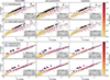 |
Fig. 5. Comparison of UVJ diagrams for galaxies with z < 2.5 (top six panels) and 2.5 ≤ z < 6 (bottom six panels) for mass-complete sample (M* ≥ 108 M⊙) from different runs. The squares are sized logarithmically according to the number of galaxies in the bin. We colour-coded the median attenuation in V-band (AV) as the histogram in the background. The grey crosses represent the QGCs selected with sSFR criterion. The dashed blue line shows the redshift-dependent criterion for quiescence by Antwi-Danso et al. (2023). We marked the fraction of QGCs (sSFR criterion) caught by UVJ criterion in the lower right corner of each panel. Top panels: Results from the MIRI run. Bottom panels: Results from the no-MIRI run. The columns are related to the SFH model used in the run, from left to right: DelayedBQ, non-parametric, and regulator. Additionally, we included galaxies we were able to recover as QGs using the Koprowski et al. (2024) MS offset criteria, with cyan crosses marking QGs from Carnall et al. (2023a) and magenta stars marking QGs from Long et al. (2024). For details, see Appendix G. |
We constructed the UVJ diagrams using the CIGALE results from each of the runs. They reflect the known correlation between the rest-frame colours and AV (increase with higher colours values) and sSFR (decrease with lower V–J and higher U–V colours; see Williams et al. 2009; Martis et al. 2019; Akins et al. 2022). However, there are significant differences among the selected samples of QGCs. We test the bias between the UVJ, MS offset, and sSFR criteria. The results are presented in Table 1.
Comparison of selected QGCs in the final sample and low-z sample.
Up to ∼20% of QGCs (selected with the sSFR criterion) display properties that are inconsistent with being an SFG according to the UVJ selection (UVJ unselected, hereafter) proposed by Antwi-Danso et al. (2023). With the delayedBQ and non-parametric SFH models, MIRI points enlarge the number of UVJ unselected, while the opposite effect is observed with the regulator model. This is true for both the entire sample and the sample restricted to z < 2.5 (see Table 1).
When selecting QGCs based on their MS distance (as defined in Koprowski et al. 2024), the fraction of QGCs that are not selected by the UVJ criterion is strongly biased by both SFH and MIRI. Firstly, MIRI points tend to always increase the number of QGCs not selected by UVJ, exposing the fact that UVJ does not completely break the degeneracy of sSFH-AV. Secondly, the fraction of UVJ unselected QGCs is always slightly lower in the sample restricted to z < 2.5 than in the entire sample. This is in agreement with recent studies showing that UVJ does not have the capacity to separate QGCs from the other galaxies for high-z galaxies (z > 3) due to still relatively young stellar populations (Antwi-Danso et al. 2023; Lovell et al. 2023; Valentino et al. 2023; Long et al. 2024). Finally, the number of QGCs not selected by UVJ is strongly dependent on SFH and is the highest for non-parametric model, reaching 69%. The regulator model is the most consistent with the Schreiber et al. (2015) UVJ criterion, but the fraction of QGCs not selected by UVJ can still reach 14%.
We confirm that our selection methodology successfully recovers the known and spectroscopically confirmed QGs at high-z from Carnall et al. (2023a) and the QGs studied in Long et al. (2024). For a detailed description, we refer to Appendix G. In summary, we find that three sources from Carnall et al. (2023a) and eight sources from Long et al. (2024) are present in our final sample (the rest were not included in MIRI pointings). We recover similar M★ (±0.3 dex) and we are able to recover the quiescent nature of all three Carnall et al. (2023a) galaxies and five or six (depending on the SFH model) out of nine Long et al. (2024) galaxies using the Koprowski et al. (2024) MS offset criterion. All recovered QGs are marked in Fig. 5.
We find that the mean AV increases with M★ for SFGs (non-QGCs) in all runs in both redshift bins. Our results in redshift z < 2.5 align perfectly with the relation presented by van der Wel et al. (2025). The V-J colour increases with AV values, and low- and intermediate-mass galaxies (M* < 1010 M⊙) tend to have AV < 1 mag. For galaxies with M* > 1011 M⊙, the mean AV reaches ∼3 mag. Although this trend is also visible for QGCs in all runs, the AV increases only by 0.26, 0.3 and 0.25 mag within the MIRI run for the delayedBQ, non-parametric, and regulator models, respectively (see Fig. 6).
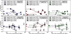 |
Fig. 6. Relation between time since quenching (ΔT) and the AV of the mass-complete QGCs at z ≤ 2.5. The columns show different SFH models used in the run, from left to right: DelayedBQ, non-parametric, and regulator, while the rows show the MIRI vs no-MIRI runs. The colours represent the median M★ of each bins. The arrows on the left of each panel show the weighted mean for the corresponding M★ bin. |
4.4. Inferring quenching-related parameters from the SFH
Finally, we have drawn insights into the quenching properties and timescales recovered by our photometry-fitted SFH models. For this purpose, we prepared and studied the sSFH for each QGC selected by the sSFR criterion. The description of the sSFH calculation can be found in Appendix E. In short, we recreated the M★ growth curve according to SFH and divided the SFH by the M★ growth curve to obtain sSFR in each time step. Here, we used low-z part of our sample (z ≤ 2.5), as the sSFR-based criterion was not calibrated for higher redshifts, while MIRI fluxes directly probe the warm dust emission within this redshift range.
For each QGC, we define three key quenching timescales to quantify the temporal changes of the SFR: (1) quenching moment, τq; (2) quenching time, Tq; (3) time since quenching, ΔT. A visual interpretation is given in Fig. 1. It is worth mentioning that the examples in the figure are not representative of the low- and high-mass populations. The τq value gives the cosmic time when the galaxy is considered quenched (the sSFR of the galaxy goes below 0.2/τ(z), where τ(z) is the cosmic time at a given redshift). To account for stochastic changes in SFR changes, we followed Lorenzon et al. (2025a) and required the sSFR to remain below the threshold for a minimum time of 0.2 × τ(zq), where zq is the redshift to fall below the threshold. The Tq is the time the galaxy spends between two thresholds defined as 1/τ(z) and 0.2/τ(z), with examples given in Appendix F). In other words, Tq describes how rapid the quenching process was. The ΔT is the look-back time since the quenching moment (ΔT ≡τ(zo)−τq, where zo is the observed redshift of the galaxy).
We studied the consistency amongst quenching parameters defined above in the way described in Sect. 4.2 and Appendix D. We used the five best fits per galaxy (see Sect. 3.2). We performed a stability analysis for the regulator model only, since it is free of instant quenching processes. The 90th percentile, P90 of the CV distribution of quenching time (τq) is at ∼43%. The influence of redshift on the stability of τq is negligible. Thus, the τq recovered by individual runs can vary at the level of < 45%. The P90 of the Tq CV distribution is at ∼199%; thus, Tq does not converge to the same value and the estimate is not stable.
By comparing the recovered timescales to those found in cosmological simulations for objects selected in the same way, we can confirm their physical meaning. For this purpose, we used an exemplary simulated galaxy from SIMBA (for details, see Appendix F). We report that the value of τq is consistent within 2σ (with σ ∼ 8% of the value), compared to the simulated SFH. Although the value of Tq from the best fit is consistent with the one obtained directly from the simulation, it again does not converge to the same value as σ ∼ 67%. Thus, due to the large scatter in the observational sample and in the SED modelling of the simulated galaxy, we do not recommend using Tq with photometry-only studies.
4.5. Considering whether QGCs could be dust attenuated
In the MIRI run, using the sSFR criterion, we find 16 (13%), 24 (14%), and 4 (4%) QGCs with AV > 1 for the delayedBQ, non-parametric, and regulator SFH models, respectively; percentages are relative to the total number of QGCs per model. In Fig. 1 we present the ranges for observational fluxes depending on attenuation, as well as the number of sources in the four attenuation bins for MIRI run with the regulator SFH. In the o–MIRI run, for the same combination of SFH models, we find 9 (10%), 10 (11%), and 3 (9%) QGCs with AV > 1. It is clear that both the absolute counts and the fractions of dusty QGCs are lower without MIRI, underscoring the importance of MIR constraints for robust AV estimates and sample classification. These results also indicate that QGs can maintain a significant amount of dust after quenching. This points to mechanisms that can help retain (or even rebuild) the dust reservoir in quenched objects. In the literature, there is a growing number of studies identifying dusty QGCs across redshifts (see Donevski et al. 2023; Setton et al. 2024; Siegel et al. 2025; Bevacqua et al. 2025; Lorenzon et al. 2025b), but the mechanisms behind their dusty nature are not yet fully understood (Lorenzon et al. 2025a).
In Fig. 6 we show the evolution of AV as a function of time since quenching for selected QGCs at z ≤ 2.5 and considering all combinations of SFHs and inclusion and exclusion of MIRI data. We studied a mass-complete sample. The QGCs are divided into three M★ bins of similar size. In each M★ bin, the QGCs are divided into four ΔT sub-bins of similar size (the number of QGCs in sub-bins is always ≥6). The ranges of M★ and ΔT for each sub-bin are presented in Table H.1. In each sub-bin, we calculated the median value of ΔT and AV. The error bars represent the standard deviation of the bootstrap analysis, a resampling method to estimate the statistical uncertainties of the measurements combined with intrinsic uncertainties. We resampled our data set for 1 000 random samples with three random objects removed from the entire sample of mass-complete QGCs.
Comparing the MIRI and no-MIRI runs, we can see from Fig. 6 that the addition of MIRI points and dust emission models reduces the median AV in all M★ bins. We discuss the constraining of AV according to the CIGALE mock analysis in Appendix D.4. Despite the negligible change in AV uncertainties, consistency amongst different SFH is stable across the probed ΔT ranges. This decreased AV is more prominent towards larger ΔT and lower M★. We see a dramatic decrease in AV (0.5–1.2 mag) when MIRI data is present for the largest ΔT and least massive QGCs (M* ∼ 109 M⊙). Even if obtaining proper ages and AV is uncertain without spectroscopy (e.g. Nersesian et al. 2025), we can use rich photometry to constrain them. Therefore, it is clear that MIRI data help break the dust-age degeneracy.
Interestingly, as shown with the arrows at left of each panel of Fig. 6, the most massive bin always has the highest attenuation. A similar relation of AV as a function of M★ was reported by Gebek et al. (2025), Maheson et al. (2025) and van der Wel et al. (2025). We suspect that this is an effect of a patchy dust distribution, or dusty cores, rather than extreme dustiness (Miller et al. 2022; Setton et al. 2024; Siegel et al. 2025). Although this is true for weighted mean values, we do not see a direct evolution of AV with ΔT.
Overall, QGCs with lower M★ tend to have a larger span of ΔT. For delayedBQ and regulator runs, the distributions of ΔT in the least massive bin (M* ∼ 109 M⊙) is twice as wide as for the most massive bin (M* ∼ 1011 M⊙). For non-parametric runs, it has the same ratio only for the no-MIRI run, while for the MIRI run it is still visible, but reaches only ∼25%. This indicates distinct evolutionary paths for high- and low-mass QGCs. A similar finding was reported by Cutler et al. (2024). It might be related to the quenching mechanism, as reported for low-z galaxies (Donnari et al. 2019). Our analysis of all three MIRI runs reveals a consistent trend for sustaining substantial AV first ∼1 Gyr after quenching. This is in line with the findings and predictions of Donevski et al. (2023), Lorenzon et al. (2025a) and Lorenzon et al. (2025b).
We report that QGCs with ΔT> 1 Gyr (mature QGCs, hereafter) are the most diverse. Firstly, most mature QGCs maintain low attenuation, AV < 1 mag. This indicates that dust production is inefficient in typical QGCs or that strong destruction processes dominate the post-quenching phase. Nevertheless, the most attenuated QGCs in all runs are usually mature as well. All QGCs with AV > 1 mag within regulator MIRI run are mature. For the non-parametric MIRI run, we find that 55% of QGCs with AV > 1 mag are mature; however, this fraction rises to 77% for AV > 1.2 mag. Only the delayedBQ MIRI run results in a lower fraction of mature QGCs with AV > 1 mag, reaching 30%. These mature and attenuated QGCs had more than 1 Gyr to accumulate dust, which implies that the mechanism responsible for sustaining the dust operates on long timescales, rather than rapidly. This diversity may point to an additional mechanism that enriches the ISM with dust, as proposed in some studies (e.g. dust re-growth; Donevski et al. 2023; Lorenzon et al. 2025a) or the addition of asymptotic giant branch (AGB) stars (Michałowski et al. 2019; Bevacqua et al. 2025).
5. Summary and conclusions
We exploited the unprecedented depth of ∼29 mag of the JWST data and the wide optical-to-MIR wavelength coverage in the CEERS field to perform a comprehensive comparison of factors affecting the photometric selection of QGCs. Combining HST/JWST fluxes from the ASTRODEEP-JWST catalogue over the CEERS field (Merlin et al. 2024) with our analysis of MIRI detections and observational depths, we built a multi-wavelength (optical-MIR) catalogue of galaxies below z < 6, including MIRI upper limits. In total, we studied a mass complete sample of ∼5000 galaxies within the MIRI footprint. We have investigated how the selection of QGCs and their physical properties are impacted due to different SFH choices, including non-parametric and regulator stochastic models that we implemented within the CIGALE code. Our main results can be summarised as follows:
-
We constructed the largest so far catalogue of MIRI observed QGCs. It consists of between 103 and 180 galaxies when the most restrictive QGC selection criterion (sSFR; Pacifici et al. 2016) is used; the factor of ∼2 difference in sample size depends on the SFH model used. When the MS distance (in particular, the Koprowski et al. 2024 MS) was used as the selection criterion, the corresponding number of selected QGCs increases to 200-743.
-
Inclusion of MIRI points and dust emission models in the SED modelling is crucial for SFR estimation. It increases the number of QGCs selected by the factor 1.4 − 2, independently of the selection criteria and the SFH model used.
-
Different SFH models lead to large variations in number of selected QGCs, up to a factor of ∼3.5. The non-parametric model selects the largest samples, while the regulator model yields the smallest.
-
A significant fraction of QGCs defined by either sSFR or MS-offset were not recovered via UVJ diagrams. Incorporating MIR data and dust emission models reveals up to 69% of QGCs missed by UVJ color-criterion alone.
-
We report the importance of MIR observations in restricting AV in mature QGCs (with the time since quenching ΔT > 1 Gyr). We did not find a clear correlation between AV and ΔT. However, we find that substantial dust attenuation is sustained after the first ∼1 Gyr after quenching. This hints at an additional dust reprocessing mechanism being present in mature QGCs.
-
On average, massive QGCs (M* ∼ 1011 M⊙) have AV values greater by ∼0.3 mag as compared to the least massive QGCs in our sample (M* ∼ 109M⊙). This observation remains true for each SFH-data combination.
-
Photometry-only SED fitting codes, such as CIGALE, can recreate, to some extent, the SFH of the simulated galaxies. The precision of ΔT reaches around ∼45%, while Tq does not converge to the same value. We urge caution on using τq inferred from the SFH modelled using photometric points only.
-
Photometry alone can significantly constrain the evolution of galaxies and MIRI is fundamental to obtaining realistic AV and distinguish between QGs and SFGs.
Our results motivate QGC selection exploiting full photometric exploitation of NIRCam data with multi-band MIRI imaging surveys in deep fields, including CEERS (e.g. Muzzin et al. 2025).
Data availability
Table 2 is available at the CDS via https://cdsarc.cds.unistra.fr/viz-bin/cat/J/A+A/708/A235
Acknowledgments
We thank the anonymous referee for the careful reading of the manuscript and the useful comments improving the readability and clarifying the message. We acknowledge support from the Polish National Science Center (NCN) grants: UMO-2023/49/N/ST9/00746, UMO- 2024/53/B/ST9/00230, 2023/50/E/ST9/00383, UMO-2020/39/D/ST9/00720, UMO-2023/51/D/ST9/00147, UMO-2020/38/E/ST9/00077, 2023/50/A/ST9/00579. We acknowledge the support of the Polish Ministry of Education and Science through the grant PN/01/0034/2022 under ‘Perły Nauki’ programme. D.D. acknowledge support from the Polish National Agency for Academic Exchange (Bekker grant BPN /BEK/2024/1/00029/DEC/1). A.W.S.M. acknowledges the support of the Natural Sciences and Engineering Research Council of Canada (NSERC) through grant reference number RGPIN-2021-03046. S.B. is supported by the ERC StG 101076080. J. is funded by the European Union (MSCA EDUCADO, GA 101119830 and WIDERA ExGal-Twin, GA 101158446). C.B. acknowledges support through an Emmy Noether Grant of the German Research Foundation, a stipend by the Daimler and Benz Foundation and a Verbundforschung grant by the German Space Agency. S.D. acknowledges support through DEC-2025/09/X/ST9/01569 grant.
References
- Akhshik, M., Whitaker, K. E., Leja, J., et al. 2023, ApJ, 943, 179 [NASA ADS] [CrossRef] [Google Scholar]
- Akins, H. B., Narayanan, D., Whitaker, K. E., et al. 2022, ApJ, 929, 94 [NASA ADS] [CrossRef] [Google Scholar]
- Annunziatella, M., P’erez-Gonz’alez, P. G., Álvarez-Márquez, J., et al. 2025, A&A, 702, A224 [NASA ADS] [CrossRef] [EDP Sciences] [Google Scholar]
- Antwi-Danso, J., Papovich, C., Leja, J., et al. 2023, ApJ, 943, 166 [NASA ADS] [CrossRef] [Google Scholar]
- Appleby, S., Davé, R., Kraljic, K., Anglés-Alcázar, D., & Narayanan, D. 2020, MNRAS, 494, 6053 [NASA ADS] [CrossRef] [Google Scholar]
- Arango-Toro, R. C., Ilbert, O., Ciesla, L., et al. 2025, A&A, 696, A159 [NASA ADS] [CrossRef] [EDP Sciences] [Google Scholar]
- Arnouts, S., Walcher, C. J., Le Fèvre, O., et al. 2007, A&A, 476, 137 [CrossRef] [EDP Sciences] [Google Scholar]
- Arnouts, S., Le Floc’h, E., Chevallard, J., et al. 2013, A&A, 558, A67 [NASA ADS] [CrossRef] [EDP Sciences] [Google Scholar]
- Aufort, G., Laigle, C., McCracken, H. J., et al. 2025, A&A, 699, A328 [NASA ADS] [CrossRef] [EDP Sciences] [Google Scholar]
- Baker, W. M., Valentino, F., Lagos, C. d. P., et al. 2025, A&A, 702, A270 [NASA ADS] [CrossRef] [EDP Sciences] [Google Scholar]
- Balogh, M. L., Morris, S. L., Yee, H. K. C., Carlberg, R. G., & Ellingson, E. 1999, ApJ, 527, 54 [Google Scholar]
- Beichman, C. A., Rieke, M., Eisenstein, D., et al. 2012, in SPIE Conf. Ser., 8442, 84422N [Google Scholar]
- Belli, S., Newman, A. B., & Ellis, R. S. 2019, ApJ, 874, 17 [Google Scholar]
- Bertin, E. 2011, ASP Conf. Ser., 442, 435 [Google Scholar]
- Bertin, E., & Arnouts, S. 1996, A&AS, 117, 393 [NASA ADS] [CrossRef] [EDP Sciences] [Google Scholar]
- Bevacqua, D., Saracco, P., La Barbera, F., et al. 2025, A&A, 699, A203 [NASA ADS] [CrossRef] [EDP Sciences] [Google Scholar]
- Bezanson, R., Spilker, J. S., Suess, K. A., et al. 2022, ApJ, 925, 153 [NASA ADS] [CrossRef] [Google Scholar]
- Boquien, M., Burgarella, D., Roehlly, Y., et al. 2019, A&A, 622, A103 [NASA ADS] [CrossRef] [EDP Sciences] [Google Scholar]
- Bouchet, P., García-Marín, M., Lagage, P. O., et al. 2015, PASP, 127, 612 [CrossRef] [Google Scholar]
- Bradley, L., Sipőcz, B., Robitaille, T., et al. 2023, https://doi.org/10.5281/zenodo.1035865 [Google Scholar]
- Brammer, G. B., Sánchez-Janssen, R., Labbé, I., et al. 2012, ApJ, 758, L17 [NASA ADS] [CrossRef] [Google Scholar]
- Bruzual, A. G. 1983, ApJ, 273, 105 [CrossRef] [Google Scholar]
- Bruzual, G., & Charlot, S. 2003, MNRAS, 344, 1000 [NASA ADS] [CrossRef] [Google Scholar]
- Carnall, A. C., Leja, J., Johnson, B. D., et al. 2019, ApJ, 873, 44 [Google Scholar]
- Carnall, A. C., McLeod, D. J., McLure, R. J., et al. 2023a, MNRAS, 520, 3974 [NASA ADS] [CrossRef] [Google Scholar]
- Carnall, A. C., McLure, R. J., Dunlop, J. S., et al. 2023b, Nature, 619, 716 [NASA ADS] [CrossRef] [Google Scholar]
- Carvajal-Bohorquez, C., Ciesla, L., Laporte, N., et al. 2025, A&A, 704, A290 [NASA ADS] [CrossRef] [EDP Sciences] [Google Scholar]
- Chabrier, G. 2003, PASP, 115, 763 [Google Scholar]
- Charlot, S., & Fall, S. M. 2000, ApJ, 539, 718 [Google Scholar]
- Cheng, C. M., Kriek, M., Beverage, A. G., et al. 2025, MNRAS, 540, 1527 [Google Scholar]
- Chien, T. C. C., Ling, C.-T., Goto, T., et al. 2024, MNRAS, 532, 719 [Google Scholar]
- Ciesla, L., Boselli, A., Elbaz, D., et al. 2016, A&A, 585, A43 [NASA ADS] [CrossRef] [EDP Sciences] [Google Scholar]
- Ciesla, L., Buat, V., Boquien, M., et al. 2021, A&A, 653, A6 [NASA ADS] [CrossRef] [EDP Sciences] [Google Scholar]
- Ciesla, L., Gómez-Guijarro, C., Buat, V., et al. 2023, A&A, 672, A191 [NASA ADS] [CrossRef] [EDP Sciences] [Google Scholar]
- Cole, J. W., Papovich, C., Finkelstein, S. L., et al. 2025, ApJ, 979, 193 [Google Scholar]
- Conroy, C. 2013, ARA&A, 51, 393 [NASA ADS] [CrossRef] [Google Scholar]
- Cutler, S. E., Whitaker, K. E., Weaver, J. R., et al. 2024, ApJ, 967, L23 [NASA ADS] [CrossRef] [Google Scholar]
- Daddi, E., Renzini, A., Pirzkal, N., et al. 2005, ApJ, 626, 680 [NASA ADS] [CrossRef] [Google Scholar]
- Davé, R., Thompson, R., & Hopkins, P. F. 2016, MNRAS, 462, 3265 [Google Scholar]
- Davé, R., Anglés-Alcázar, D., Narayanan, D., et al. 2019, MNRAS, 486, 2827 [Google Scholar]
- Donevski, D., Lapi, A., Małek, K., et al. 2020, A&A, 644, A144 [NASA ADS] [CrossRef] [EDP Sciences] [Google Scholar]
- Donevski, D., Damjanov, I., Nanni, A., et al. 2023, A&A, 678, A35 [NASA ADS] [CrossRef] [EDP Sciences] [Google Scholar]
- Donnari, M., Pillepich, A., Nelson, D., et al. 2019, MNRAS, 485, 4817 [Google Scholar]
- Draine, B. T., Aniano, G., Krause, O., et al. 2014, ApJ, 780, 172 [Google Scholar]
- Elbaz, D., Leiton, R., Nagar, N., et al. 2018, A&A, 616, A110 [NASA ADS] [CrossRef] [EDP Sciences] [Google Scholar]
- Faber, S. M., Willmer, C. N. A., Wolf, C., et al. 2007, ApJ, 665, 265 [Google Scholar]
- Fang, J. J., Faber, S. M., Koo, D. C., et al. 2018, ApJ, 858, 100 [NASA ADS] [CrossRef] [Google Scholar]
- Feldmann, R., & Mayer, L. 2015, MNRAS, 446, 1939 [Google Scholar]
- Finkelstein, S. L., Bagley, M. B., Arrabal Haro, P., et al. 2022, ApJ, 940, L55 [NASA ADS] [CrossRef] [Google Scholar]
- Finlator, K., Davé, R., & Oppenheimer, B. D. 2007, MNRAS, 376, 1861 [Google Scholar]
- Franzetti, P., Scodeggio, M., Garilli, B., et al. 2007, A&A, 465, 711 [NASA ADS] [CrossRef] [EDP Sciences] [Google Scholar]
- Fumagalli, M., Labbé, I., Patel, S. G., et al. 2014, ApJ, 796, 35 [Google Scholar]
- Gebek, A., Diemer, B., Martorano, M., et al. 2025, A&A, 695, A90 [NASA ADS] [CrossRef] [EDP Sciences] [Google Scholar]
- Glazebrook, K., Schreiber, C., Labbé, I., et al. 2017, Nature, 544, 71 [Google Scholar]
- Gobat, R., Daddi, E., Magdis, G., et al. 2018, Nat. Astron., 2, 239 [NASA ADS] [CrossRef] [Google Scholar]
- Gould, K. M. L., Brammer, G., Valentino, F., et al. 2023, AJ, 165, 248 [NASA ADS] [CrossRef] [Google Scholar]
- Haines, C. P., Iovino, A., Krywult, J., et al. 2017, A&A, 605, A4 [NASA ADS] [CrossRef] [EDP Sciences] [Google Scholar]
- Iglesias-Navarro, P., Huertas-Company, M., Martín-Navarro, I., Knapen, J. H., & Pernet, E. 2024, A&A, 689, A58 [NASA ADS] [CrossRef] [EDP Sciences] [Google Scholar]
- Ilbert, O., McCracken, H. J., Le Fèvre, O., et al. 2013, A&A, 556, A55 [NASA ADS] [CrossRef] [EDP Sciences] [Google Scholar]
- Iyer, K., & Gawiser, E. 2017, ApJ, 838, 127 [NASA ADS] [CrossRef] [Google Scholar]
- Iyer, K. G., Gawiser, E., Faber, S. M., et al. 2019, ApJ, 879, 116 [NASA ADS] [CrossRef] [Google Scholar]
- Iyer, K. G., Tacchella, S., Genel, S., et al. 2020, MNRAS, 498, 430 [NASA ADS] [CrossRef] [Google Scholar]
- Iyer, K. G., Speagle, J. S., Caplar, N., et al. 2024, ApJ, 961, 53 [NASA ADS] [CrossRef] [Google Scholar]
- Kauffmann, G., Heckman, T. M., White, S. D. M., et al. 2003, MNRAS, 341, 33 [Google Scholar]
- Kennicutt, R. C., Jr 1992, ApJ, 388, 310 [CrossRef] [Google Scholar]
- Koprowski, M. P., Wijesekera, J. V., Dunlop, J. S., et al. 2024, A&A, 691, A164 [NASA ADS] [CrossRef] [EDP Sciences] [Google Scholar]
- Kriek, M., van der Wel, A., van Dokkum, P. G., Franx, M., & Illingworth, G. D. 2008, ApJ, 682, 896 [NASA ADS] [CrossRef] [Google Scholar]
- Krywult, J., Tasca, L. A. M., Pollo, A., et al. 2017, A&A, 598, A120 [NASA ADS] [CrossRef] [EDP Sciences] [Google Scholar]
- Lee, M. M., Steidel, C. C., Brammer, G., et al. 2024, MNRAS, 527, 9529 [Google Scholar]
- Leja, J., Carnall, A. C., Johnson, B. D., Conroy, C., & Speagle, J. S. 2019a, ApJ, 876, 3 [Google Scholar]
- Leja, J., Tacchella, S., & Conroy, C. 2019b, ApJ, 880, L9 [NASA ADS] [CrossRef] [Google Scholar]
- Lisiecki, K., Małek, K., Siudek, M., et al. 2023, A&A, 669, A95 [NASA ADS] [CrossRef] [EDP Sciences] [Google Scholar]
- Long, A. S., Antwi-Danso, J., Lambrides, E. L., et al. 2024, ApJ, 970, 68 [Google Scholar]
- Looser, T. J., D’Eugenio, F., Maiolino, R., et al. 2024, Nature, 629, 53 [Google Scholar]
- Lorenzon, G., Donevski, D., Lisiecki, K., et al. 2025a, A&A, 693, A118 [NASA ADS] [CrossRef] [EDP Sciences] [Google Scholar]
- Lorenzon, G., Donevski, D., Man, A. W. S., et al. 2025b, ApJ, 995, L63 [Google Scholar]
- Lovell, C. C., Roper, W., Vijayan, A. P., et al. 2023, MNRAS, 525, 5520 [NASA ADS] [Google Scholar]
- Lower, S., Narayanan, D., Leja, J., et al. 2020, ApJ, 904, 33 [NASA ADS] [CrossRef] [Google Scholar]
- Lu, S., Daddi, E., Maraston, C., et al. 2025, Nat. Astron., 9, 128 [Google Scholar]
- Madau, P., & Dickinson, M. 2014, ARA&A, 52, 415 [Google Scholar]
- Maheson, G., Tacchella, S., Belli, S., et al. 2025, MNRAS, submitted [arXiv:2504.15346] [Google Scholar]
- Małek, K., Junais, Pollo, A., et al. 2024, A&A, 684, A30 [NASA ADS] [CrossRef] [EDP Sciences] [Google Scholar]
- Man, A., & Belli, S. 2018, Nat. Astron., 2, 695 [NASA ADS] [CrossRef] [Google Scholar]
- Martis, N. S., Marchesini, D. M., Muzzin, A., et al. 2019, ApJ, 882, 65 [NASA ADS] [CrossRef] [Google Scholar]
- Mathis, H., Charlot, S., & Brinchmann, J. 2006, MNRAS, 365, 385 [Google Scholar]
- Mérida, R. M., Sawicki, M., Iyer, K. G., et al. 2026, A&A, 707, A5 [NASA ADS] [CrossRef] [EDP Sciences] [Google Scholar]
- Merlin, E., Santini, P., Paris, D., et al. 2024, A&A, 691, A240 [NASA ADS] [CrossRef] [EDP Sciences] [Google Scholar]
- Merlin, E., Fortuni, F., Calabró, A., et al. 2025, Open J. Astrophys., 8, E170 [Google Scholar]
- Michałowski, M. J., Hjorth, J., Gall, C., et al. 2019, A&A, 632, A43 [NASA ADS] [CrossRef] [EDP Sciences] [Google Scholar]
- Miller, T. B., Whitaker, K. E., Nelson, E. J., et al. 2022, ApJ, 941, L37 [NASA ADS] [CrossRef] [Google Scholar]
- Mintz, A., Setton, D. J., Greene, J. E., et al. 2026, ApJ, 998, 257 [Google Scholar]
- Morishita, T., Abdurro’uf, Hirashita, H., et al. 2022, ApJ, 938, 144 [Google Scholar]
- Muzzin, A., Suess, K. A., Marchesini, D., et al. 2025, ApJS, submitted [arXiv:2507.19706] [Google Scholar]
- Nagaraj, G., Forbes, J. C., Leja, J., Foreman-Mackey, D., & Hayward, C. C. 2022, ApJ, 939, 29 [NASA ADS] [CrossRef] [Google Scholar]
- Narayanan, D., Turk, M. J., Robitaille, T., et al. 2021, ApJS, 252, 12 [NASA ADS] [CrossRef] [Google Scholar]
- Nersesian, A., van der Wel, A., Gallazzi, A. R., et al. 2025, A&A, 695, A86 [NASA ADS] [CrossRef] [EDP Sciences] [Google Scholar]
- Ocvirk, P., Pichon, C., Lançon, A., & Thiébaut, E. 2006, MNRAS, 365, 46 [Google Scholar]
- Pacifici, C., Kassin, S. A., Weiner, B. J., et al. 2016, ApJ, 832, 79 [Google Scholar]
- Patel, S. G., Kelson, D. D., Holden, B. P., Franx, M., & Illingworth, G. D. 2011, ApJ, 735, 53 [NASA ADS] [CrossRef] [Google Scholar]
- Patel, S. G., Holden, B. P., Kelson, D. D., et al. 2012, ApJ, 748, L27 [NASA ADS] [CrossRef] [Google Scholar]
- Pearson, W. J., Pistis, F., Figueira, M., et al. 2023, A&A, 679, A35 [NASA ADS] [CrossRef] [EDP Sciences] [Google Scholar]
- Peng, C. Y., Ho, L. C., Impey, C. D., & Rix, H.-W. 2002, AJ, 124, 266 [Google Scholar]
- Popesso, P., Concas, A., Cresci, G., et al. 2023, MNRAS, 519, 1526 [Google Scholar]
- Price, S. H., Kriek, M., Brammer, G. B., et al. 2014, ApJ, 788, 86 [NASA ADS] [CrossRef] [Google Scholar]
- Riccio, G., Małek, K., Nanni, A., et al. 2021, A&A, 653, A107 [NASA ADS] [CrossRef] [EDP Sciences] [Google Scholar]
- Rieke, G. H., Wright, G. S., Böker, T., et al. 2015, PASP, 127, 584 [NASA ADS] [CrossRef] [Google Scholar]
- Rodríguez Montero, F., Davé, R., Wild, V., Anglés-Alcázar, D., & Narayanan, D. 2019, MNRAS, 490, 2139 [CrossRef] [Google Scholar]
- Santini, P., Ferguson, H. C., Fontana, A., et al. 2015, ApJ, 801, 97 [Google Scholar]
- Schreiber, C., Pannella, M., Elbaz, D., et al. 2015, A&A, 575, A74 [NASA ADS] [CrossRef] [EDP Sciences] [Google Scholar]
- Setton, D. J., Khullar, G., Miller, T. B., et al. 2024, ApJ, 974, 145 [Google Scholar]
- Siegel, J. C., Setton, D. J., Greene, J. E., et al. 2025, ApJ, 985, 125 [Google Scholar]
- Simmonds, C., Tacchella, S., McClymont, W., et al. 2025, MNRAS, 544, 4551 [Google Scholar]
- Siudek, M., Małek, K., Scodeggio, M., et al. 2017, A&A, 597, A107 [NASA ADS] [CrossRef] [EDP Sciences] [Google Scholar]
- Smith, D. J. B., & Hayward, C. C. 2015, MNRAS, 453, 1597 [NASA ADS] [CrossRef] [Google Scholar]
- Speagle, J. S., Steinhardt, C. L., Capak, P. L., & Silverman, J. D. 2014, ApJS, 214, 15 [Google Scholar]
- Stefanon, M., Yan, H., Mobasher, B., et al. 2017, ApJS, 229, 32 [NASA ADS] [CrossRef] [Google Scholar]
- Strateva, I., Ivezić, Ž., Knapp, G. R., et al. 2001, AJ, 122, 1861 [CrossRef] [Google Scholar]
- Tacchella, S., Forbes, J. C., & Caplar, N. 2020, MNRAS, 497, 698 [Google Scholar]
- Tacchella, S., Conroy, C., Faber, S. M., et al. 2022, ApJ, 926, 134 [NASA ADS] [CrossRef] [Google Scholar]
- Valentino, F., Tanaka, M., Davidzon, I., et al. 2020, ApJ, 889, 93 [Google Scholar]
- Valentino, F., Brammer, G., Gould, K. M. L., et al. 2023, ApJ, 947, 20 [NASA ADS] [CrossRef] [Google Scholar]
- van der Wel, A., Martorano, M., Marchesini, D., et al. 2025, A&A, 701, A30 [NASA ADS] [CrossRef] [EDP Sciences] [Google Scholar]
- Villa-Vélez, J. A., Buat, V., Theulé, P., Boquien, M., & Burgarella, D. 2021, A&A, 654, A153 [NASA ADS] [CrossRef] [EDP Sciences] [Google Scholar]
- Walcher, J., Groves, B., Budavári, T., & Dale, D. 2011, Ap&SS, 331, 1 [NASA ADS] [CrossRef] [Google Scholar]
- Wan, J. T., Tacchella, S., Johnson, B. D., et al. 2024, MNRAS, 532, 4002 [Google Scholar]
- Wang, E., & Lilly, S. J. 2020, ApJ, 895, 25 [Google Scholar]
- Wang, T.-M., Magnelli, B., Schinnerer, E., et al. 2022, A&A, 660, A142 [NASA ADS] [CrossRef] [EDP Sciences] [Google Scholar]
- Wang, T., Sun, H., Zhou, L., et al. 2025, ApJ, 988, L35 [Google Scholar]
- Weibel, A., de Graaff, A., Setton, D. J., et al. 2025, ApJ, 983, 11 [Google Scholar]
- Whitaker, K. E., Labbé, I., van Dokkum, P. G., et al. 2011, ApJ, 735, 86 [Google Scholar]
- Whitaker, K. E., van Dokkum, P. G., Brammer, G., et al. 2013, ApJ, 770, L39 [NASA ADS] [CrossRef] [Google Scholar]
- Whitaker, K. E., Narayanan, D., Williams, C. C., et al. 2021, ApJ, 922, L30 [NASA ADS] [CrossRef] [Google Scholar]
- Williams, R. J., Quadri, R. F., Franx, M., van Dokkum, P., & Labbé, I. 2009, ApJ, 691, 1879 [NASA ADS] [CrossRef] [Google Scholar]
- Williams, R. J., Quadri, R. F., Franx, M., et al. 2010, ApJ, 713, 738 [NASA ADS] [CrossRef] [Google Scholar]
- Willmer, C. N. A., Faber, S. M., Koo, D. C., et al. 2006, ApJ, 647, 853 [Google Scholar]
- Wu, P.-F., van der Wel, A., Bezanson, R., et al. 2018, ApJ, 868, 37 [NASA ADS] [CrossRef] [Google Scholar]
- Wuyts, S., Labbé, I., Franx, M., et al. 2007, ApJ, 655, 51 [NASA ADS] [CrossRef] [Google Scholar]
- Yang, G., Caputi, K. I., Papovich, C., et al. 2023a, ApJ, 950, L5 [NASA ADS] [CrossRef] [Google Scholar]
- Yang, G., Papovich, C., Bagley, M. B., et al. 2023b, ApJ, 956, L12 [NASA ADS] [CrossRef] [Google Scholar]
- Zheng, Y., Dave, R., Wild, V., & Montero, F. R. 2022, MNRAS, 513, 27 [NASA ADS] [CrossRef] [Google Scholar]
MIRI data that were not used in photo−z estimation. We provide a test of the influence of MIRI data on photo-z estimation in Appendix D.3, showing that there is no systematic shift.
We share our full photometric catalogue of HST/NIRCam/MIRI sources at our GitHub repository (github.com/lisieckik/CIGALE_QGs).
We note that 2614 objects reside at z < 2.5, where MIRI fluxes probe emission from warm dust and PAHs.
Ancillary files/Prepare_sSFR.py
Appendix A: Completeness analysis
To estimate the M★ completeness, we start with estimating the 90% completeness in apparent magnitude (see Fig. A.1, top-left panel). For this, we use estimates from Merlin et al. (2024) and we interpolate the curve using the cubic spline algorithm and find where the completeness curve falls below 0.9, mag90% = 29.04. Then we use two distinct methods to translate the apparent magnitude to M★.
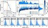 |
Fig. A.1. Completeness analysis using the first method with the regulator MIRI run results. Top left: Apparent magnitude completeness curve. The red points are values from (Merlin et al. 2024), the blue line is the interpolated curve, and the dashed orange line is the value for 90% completeness. Top right: M★-redshift plane with histograms. In grey we mark galaxies below the mag90% limit, while the white to blue colours represent the apparent magnitude of each galaxy. The red lines show the 90% completeness for each redshift bin. Bottom panels: Histograms for each of the redshift bins. The estimated maximum of the distribution is shown with dashed red lines. The median redshift of the galaxies in bin is given a the top of each panel with the maximum of the distribution. |
For the first method, we select from our photometric catalogue of 12 939 galaxies only the sources with apparent magnitude (F356W + F444W) above the 90% completeness limit. Then we divide the sample into seven logarithmic redshift bins between 0.05 and 6. For each bin, we prepare 20 M★ histograms, each with a different number of bins between 15 and 35. For each histogram, we find the M★ for which the distribution breaks (maximum of the distribution). Finally, we take the maximum value of M★ from all histograms for a given redshift range as a 90% completeness limit. We report the log(M*/M⊙) limit for 90% completeness to be 7.9, 7.8, and 7.9 for the delayedBQ, non-parametric, and regulator MIRI runs, respectively. This method is visualised in Fig. A.1.
For the second method, we utilise the stellar emission from the SEDs produced by CIGALE for all galaxies from our photometric catalogue of 12 939 galaxies. The SEDs are corrected to the rest-frame and redshifted for z = 0 + 0.05n, with n = 1, 2, 3...200 (up to z = 10). Each of the redshifted SEDs is then convolved with a transmission curve of F356W and F444W to calculate the apparent magnitude. For each of the SEDs we find the maximum redshift for detection above 90% completeness (the apparent magnitude of F356W + F444W greater than 29.04 mag). We build two groups of galaxies:
![Mathematical equation: $$ \begin{aligned} \begin{aligned}&\mathrm{Quiescent: }\log (\mathrm{sSFR}[\mathrm{M}_\odot /\mathrm{yr}]) < -11,\\&\mathrm{Star-forming: }-9>\log (\mathrm{sSFR}[\mathrm{M}_\odot /\mathrm{yr}])>-11.\\ \end{aligned} \end{aligned} $$](/articles/aa/full_html/2026/04/aa57118-25/aa57118-25-eq3.gif) (A.1)
(A.1)
Then both groups are split into 0.5 wide redshift bins. We find the maximum M★ in each bin and fit a linear function to the results. We report the completeness of 90% in z = 6 in M* = 107.9 and = 107.6 M⊙ for the quiescent sample and the star-forming sample, respectively. The results are presented in Fig. A.2. Both methods are coherent and we can state that at z = 6 our sample is 90% complete for M* ≃ 108M⊙.
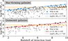 |
Fig. A.2. M★ as a function of maximum redshift for detection above 90% completeness. Top: Results for SFGs. Bottom: Results for QGs. The grey points are individual galaxies. The larger blue and red points present the largest M★ in each redshift bin. The solid blue and red lines show the linear fit, while the dashed orange line present the M★ at z = 6 according to the fit. |
Appendix B: MIRI source extraction
We use original images from the CEERS repository for public release 0.65. Using Photutils. Background2D class (Bradley et al. 2023) with MedianBackground method and SigmaClip with sigma value of three, we calculate both background maps and RMS maps. Using SExtractor with default parameters and PSF Extractor (PSFEx; Bertin 2011), we extract empirical point spread functions (PSFs) using stars within the field of view for each MIRI filter used in CEERS.
With extracted PSFs and GALFIT (Peng et al. 2002), we prepared the model point-like sources with magnitude span 23–28 separated by 0.1 mag. We then inserted 20 artificial (model) sources into empty spaces in the images and ran SExtractor, with extracted PSFs, to check which fraction of model sources is detectable. As an empty space, we considered the point in the image with a distance to all sources (which is real, previously inserted, and larger than twice the radius of the emission, using the parameter FLUX_RADIUS for SExtractor sources or 15 pixels for the artificial sources). As a detection, we considered a source extracted by SExtractor with a distance from the inserted position of less than 5 pixels (∼0.45 arcsec). We repeated the procedure 20 times per model source (in total, we inserted each model 400 times).
We present the results in the form of completeness curves in Fig. B.1, and as 5σ upper limits in Table B.2. The upper limits are estimated by fitting linear function on the completeness points between 0.3 − 0.7 values and calculating the magnitude for which the completeness is 0.5. It is worth noticing, observations with the same filter (e.g. F770W) can have different depths depending on the pointing. However, this is consistent with the integration time in each pointing.
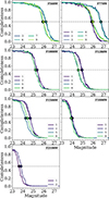 |
Fig. B.1. Completeness curves for MIRI observations from the CEERS program. Each panel represents different band, which is written in the upper-right corner. Each coloured line represents MIRI pointing. The dashed grey line marks completeness of 50%, and the circles show the estimated 5σ upper limit. |
Finally, we perform the final SExtractor run with extracted PSFs, RMS maps as WEIGHT_TYPE and other parameters specified in Table B.1. For each detection, we check if the ratio of flux (calculated from MAG_AUTO) to error (calculated from MAGERR_AUTO) is greater than 3. If the fraction is lower, we report a 5 σ upper limit as reported in Table B.2.
Summary of SExtractor input.
5σ detections in magnitudes through the MIRI imaging in CEERS.
Appendix C: CIGALE and the implementation of stochastic SFHs
C.1. Stochastic SFH I – Non-parametric
The first stochastic SFH model that we test in our SED fitting process with CIGALE (Sect. 3.2) is referred to as non-parametric. We follow the approach described by Leja et al. (2019a) with prior continuity. The continuity prior constrains the ratio of SFRs between the consecutive time-steps. This approach results in reduced burstiness, that is, fewer rapid changes in the SFR over time. The SFR changes follow the Student-t distribution, which is described by
 (C.1)
(C.1)
where Γ is the Gamma function, ν is the degree of freedom, and σt is the scale factor. Since with Student-t distribution, outliers are more likely to occur, it probes a broader range of SFH models than the Gaussian distribution. Using this distribution, we calculate the value of SFR as following:
 (C.2)
(C.2)
where n is the index of the time step and x is a random value from the Student-t distribution. For n = 1 we set SFRn = 1 for numerical simplicity, since the total SFH is later normalised.
We call this approach non-parametric; however, we are obliged to use several parameters. In our implementation, we allowed for five parameters (an exemplary set of parameters can be found in Table C.1) in the non-parametric method. The first one, age_form, is simply the look-back time of the formation of the observed galaxy, when the star formation starts. The second, nModels, controls how many SFHs should be prepared with posteriors of the Student-t distribution to test by CIGALE (each is then convolved with stellar population synthesis and enter a grid of models). The next one scaleFactor, controls σt of the Student t distribution (see Eq. C.1). Ocvirk et al. (2006) found that the evolutionary differences that can be observed and studied via SED in simple stellar populations are roughly proportional to their separation in logarithmic time. To follow this result and build the SFH in logarithmic time bins, we use the last two parameters nLevels and lastBin. The nLevels controls the number of SFR changes, thus we divide age_form into nLevels time steps. The first time-step is defined as 1/nLevels of age_form. The last time step is defined by lastBin. Finally, the rest of the time steps are equally spaced in logarithmic time (see Fig. 1 for visualisation).
CIGALE input.
Furthermore, we use the exact same priors for SFR changes when the only difference between the models is the age_form. In this way, we minimise the risk of forcing CIGALE to choose the non-optimal SFH model due to random sampling. In other words, if there is a run with more than one value for age_form, the priors will be sampled only once and the SFHs will be visually similar, just stretched. Following Leja et al. (2019a), we adopt ν = 2 (see Eq. C.1), as it is based on the Illustris simulation results.
C.2. Stochastic SFH II – Regulator
The second stochastic SFH model that we test in our SED fitting process with CIGALE (Sect. 3.2) is defined as an extended regulator (regulator, hereafter). We follow the approach described in Iyer et al. (2024), first introduced in Tacchella et al. (2020). The regulator SFH model is based on the control of the SFR by the assigned gas mass reservoir. The stochastic nature of the SFR is a result of (1) gas inflow/outflow rates, (2) gas cycling in equilibrium between atomic and molecular states, and (3) the formation, lifetime and disruption of GMCs.
As the gas mass budget may be affected by the processes mentioned above, we use the regulator, which includes their effect. We assume power laws to describe these effects (e.g. Iyer et al. 2020; Tacchella et al. 2020; Wang & Lilly 2020) with power spectral density (PSD):
 (C.3)
(C.3)
where f is the frequency of the process, s2 is the absolute normalisation at f = 0, and τ is the decorrelation time-scale of given process.
Gas inflow and gas cycling in equilibrium are coupled, whereas the lifetimes of GMCs are independent of them (Tacchella et al. 2020). Thus, the total PSD will have two additive elements. We calculate autocovariance function (ACF) from the total PSD using the Wiener–Khinchin theorem and describe the stochastic change of SFR using the following ACF:
 (C.4)
(C.4)
where σreg is long-term variability related to inflow and equilibrium, σdyn is the variability of the dynamical component, τflow, τeq, τdyn are timescales of gas inflow/outflow, equilibrium cycling and GMC’s lifetime, respectively, and τ is the timescale associated with the frequency f. For a detailed description of the derivation method of Eq. C.4, we refer to Tacchella et al. (2020) and Iyer et al. (2024).
The ACF is now used as a physically motivated prior for stochastic SFH. Following Iyer et al. (2024), we build SFH by assuming that at each time bin tn we can find SFRn, where n = 1, ..., N, which corresponds the multi-variate normal distribution:
 (C.5)
(C.5)
where μN is the N-vector of mean values and C(τ) is the corresponding N × N covariance matrix. In the regulator model, C(τ) is ACF(τ), for τ ≡ t − t′, for t, t′=t1, ..., tN, and tn are centres of the respective N time bins.
In our implementation, we allowed for eight parameters in the regulator model (an exemplary set of parameters can be found in Table C.1). Namely, age_form, nModels, which are exactly the same as in the non-parametric model (see Appendix C.1), nLevels, which controls in how many equal time bins age_form should be divided, and the equivalents of σreg, σdyn, τeq, τflow, and τdyn from Eq. C.4, respectively. It is worth noticing that most stochastic processes are defined with the μN = 0. Thus, following the implementation of Iyer et al. (2024) or Wan et al. (2024), we also use the same mean vector.
C.3. CIGALE input
Table C.1 presents the CIGALE input used in this study.
Appendix D: Stability of physical properties
To ensure that splitting the run into five smaller runs does not influence the analysis, we have conducted one additional run with nLevels = 1000. Comparing M*, SFR, AV and age, we find that each of them is consistent despite the method chosen (one big run, and five smaller runs). The differences are approximately ∼10-20 times smaller than the error reported by CIGALE. Additionally, the errors themselves are also consistent, within margin of ∼5% of their value.
The parametric SFH models, such as delayedBQ, always converge to the same value. This does not have to be true for the stochastic SFH. In order to probe the consistency of physical properties as outputs of our SED modelling with stochastic SFHs, we access the five (per stochastic SFH model) best resulting models for each galaxy within the final sample. We then check how stable the physical properties are between iteration with the same parameters, in other words, we wish to test to what level the model results (physical properties) are constrained.
D.1. MIRI run
We first explore fitting the full SED, including the longer-wavelength MIRI data. The M★ is well preserved in the five best resulting models for each of the different stochastic SFHs. The 90th percentile (P90) of the CV distributions is ∼1% and ∼6% for the regulator and the non-parametric SFH models, respectively. In other words, the Bayesian M★ converges to the same value up to ∼1% or ∼6% accuracy. Similarly, ages of the galaxies tend to converge to the same values with P90 of distributions ∼4% and ∼6% for the regulator and non-parametric SFH models, respectively. Even though we see that for the regulator model, the SFR is stable throughout the iterations with P90 at ∼3%, the non-parametric distribution shows much larger scatter with P90 at ∼17%. The strong variation of the SFR estimated with the non-parametric run is strongly biased due to lack of limit for the minimum SFR. The CIGALE does not record the difference between SFR = 10−3 and SFR = 10−6, in both cases the young population of stars will be negligible. Thus, the SFR of the passive galaxies in each iteration can be negligible but different. Finally, the CV distribution of AV shows a variation of 5% and 8% for the regulator and the non-parametric models, respectively.
D.2. No-MIRI run
Next we explore fitting the SED without longer wavelength MIRI data. The no-MIRI run results display similar tendencies. The P90 of the M★ CV (relative standard deviation CV = σ/μ) distributions is ∼1% and ∼6% for the regulator and the non-parametric SFH models, respectively. The ages tend to converge to the same values as P90 of the distributions ∼5% and ∼6% for the regulator and non-parametric SFH models, respectively. The CV distribution of the SFR within the regulator model has P90 at ∼3%, while within the non-parametric model, the distribution has P90 at ∼28%. The strong variation of the SFR estimated with the non-parametric run can be explained in the same way as in the previous section. The attenuation varies 5% and 7% for the regulator and the non-parametric models, respectively.
D.3. Influence of MIRI data on photometric redshift
We tested the influence of MIRI data on the estimation of photometric redshifts with CIGALE. We prepared two additional, but simpler, runs with CIGALE. Both runs use the same input parameters, differing only by the data used in the fitting: (1) the entire photometric data available in our catalogue and (2) HST and NIRCam data points only. We used 12 939 galaxies from the MIRI footprint. We checked 30 different delayed SFHs (3 tau_main and 10 age values), Chabrier (2003) IMF, dust attenuation by Charlot & Fall (2000) with 7 values of the Av_ISM and Draine et al. (2014) dust emission module with one single default output model. Finally, we allowed CIGALE to probe the redshift between 0.01 and 10 with a 0.003 redshift step.
In Fig. D.1 we present the comparison of estimated photometric redshifts for galaxies with M★ > 108M⊙ (according to run with MIRI). We report a great agreement between the estimates, with a mean value close to 0. Additionally, the parentage of outliers, defined in the same way as in Merlin et al. (2024), as galaxies with |zwithMIRI − zwithoutMIRI|/(1 + zwithMIRI) > 0.15, is also low, 2.4%. Thus, the inclusion of MIRI photometry does not provide a systematic shift. This is in agreement with a similar test provided by Wang et al. (2025).
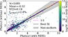 |
Fig. D.1. Photo−z estimation with and without MIRI data for galaxies with. The colour represent the stellar mass estimated in the run with MIRI data. The dashed magenta line shows 1:1 relation, while the solid black line represent the best fit. The grey shaded region show the non-outliers region defined as |zwithMIRI − zwithoutMIRI|/(1 + zwithMIRI) > 0.15. |
D.4. Influence of MIRI data on attenuation
We also test how does the AV change due to inclusion of MIRI data. For this purpose we examine the change in AV through a mock analysis included in the CIGALE. To produce the mock QGCs, the fluxes of each QGC from each run (see Sect. 4.3) are varied within the error bars, building a perfect comparison sample of the same size as the observed one. The best model is then fitted to each of the mock galaxies. Comparison of real (not varied) results with mock ones shows how constrained the physical properties given are (M★, AV, etc.). We compare AV from the real run with the mock one for mass-complete QGCs within each run (ΔAV ≡ Areal − Amock). Here we switch to the 80th percentile (P80) due to low statistics, in some bins the number of objects is less than 20.
Comparing MIRI and no-MIRI runs, we report that the P80 of the ΔAV distributions is consistently lower within the MIRI run, by 9%, 42% and 33% for delayedBQ, non-parametric, and regulator, respectively. Thus, the inclusion of MIRI data points in the SED fit helps to constrain the dust attenuation. The ΔAV is the largest in the non-parametric runs, reaching 0.26 (0.45) mag, whereas for delayedBQ it reaches 0.22 (0.24) mag and for regulator 0.18 (0.27) mag for the MIRI (no-MIRI) runs. It is important to note that this is not constant in all ΔT ranges. This difference is more important for QGCs with larger ΔT, and begins to differ significantly above ΔT∼1 Gyr. In other words, to study AV in mature QGCs, the MIR fluxes are crucial. This effect is less prominent in recently quenched galaxies.
Appendix E: Extracting the sSFH from CIGALE’s results
As discussed in Appendix D, the Bayesian set of results, such as M★ or age, seems to be consistent between runs. However, as a CIGALE output, we get only the SFH corresponding to the best fit. Thus, we need to scale it to produce the Bayesian value of M★ in the Bayesian age. We explain the process in the following, but we also include the code to calculate sSFH in the GitHub project.6
First, we place the SFR in the cosmic-time array. The CIGALE result SFH is a set of values, Tbest, from 0 to the best fit age, agebest, of the galaxy in Myr and the corresponding table SFRbest. Thus, we can place the galaxy in the cosmic time-frame for ageBayes via:
 (E.1)
(E.1)
where t(z) is cosmic time at galaxy’s observed z. In this notation Tcosmic is an array from the formation age, t(z)−agebayes, up to t(z). Finally, we can define Tcosmic, 1Myr, which has the same age range but is equally spaced by 1 Myr.
We also have to scale the SFR table, SFRbest. However, due to the different ages range in Tcosmic, we first have to interpolate the SFR values for each corresponding time step in Tcosmic, 1Myr. In effect of interpolation, SFH now forms M*, interp. Thus, we have to account for ratio of masses:
 (E.2)
(E.2)
where SFRcosmic, 1Myr is the table of SFR corresponding to Tcosmic, 1Myr. The tables are now placed in cosmic time and form exactly M*, Bayes.
To produce sSFH, we need to divide SFRcosmic, 1Myr by the stellar mass of the galaxy. To calculate the evolution of M★, we loop over each time step in Tcosmic, 1Myr and convolve the SFH up to the given time step with a single stellar population model used in our CIGALE run, calculating mass growth. We are aware this mass is only record of in situ formed stars and will differ when the stars were brought in through mergers. However, CIGALE does not include the history of mergers in the mass calculation (Iyer et al. 2019). Thus, the in situ formed galaxy is the best we can achieve using CIGALE’s SFH.
We must notice that, since we focus on reproducing Bayesian M★, the scaling can change the final SFR of the galaxy. Thus, it is possible that the galaxy selected as QGC using CIGALE Bayesian output will not meet the same criteria after SFH scaling. In our study, the difference in sample size never decreases by more than ∼3% compared to selection with use of direct CIGALE SFR values.
Appendix F: Validation of the SFH with the SIMBA galaxy
SIMBA (Davé et al. 2019) is a cutting-edge cosmological hydrodynamical simulation. It evolves baryonic matter together with dark matter and is perfectly suited for studying dust-related properties because of the self-consistent evaluation of dust destruction and growth processes at each evolutionary step. Furthermore, it implements a more realistic and careful treatment of the AGN feedback and the rich chemical evolution of ISM, compared to the previous iteration (MUFASA, Davé et al. 2016). We make use of the full-physics high-resolution simulation (m25n512) consisting of a box side 25h−1 Mpc containing 2×5123 particles. The entire run covers the redshift range 0 < z< 249. For details of the simulation, we refer to Davé et al. (2019).
In this study, we use a SIMBA simulated galaxy in order to compare direct, simulated SFH with the one estimated via SED fitting to check to what extent we can trust SFHs based purely on photometry. For this purpose, we select the largest galaxy in the simulation at z ∼ 1.5, which is similar to the maximum of the redshift distribution in our observed sample. We have coupled the SIMBA galaxy with the POWDERDAY radiative transfer code (Narayanan et al. 2021). The selection of a massive galaxy was important from the perspective of the resolution of radiative transfer calculations.
We calculate the SED of the simulated galaxy and convolve the redshifted, k-corrected SED with transmission curves of filters that can be found in CEERS pointing 1 (all HST, all NIRCam and F770W, F1000W, F1280W, F1500W, F1800W and F2100W MIRI). As an error of the flux, if possible, we assumed values of errors of the most massive, MIRI detected QGC in observed sample. Otherwise, we used 10% of the flux as an error. We use this set of fluxes as input for the exact same CIGALE run as the MIRI run described in Sect. 3.2 and in Table C.1.
We compare the SED fit from CIGALE between MIRI and no-MIRI runs (see the top panel in Fig. F.1). Without MIRI points, CIGALE estimates the AV by ∼1 mag higher than when MIRI points are included. Furthermore, age estimation from 3305, 3138 and 3062 Myr with MIRI points drops to 1713, 501, and 1737 Myr when MIRI is not used, for the delayedBQ, non-parametric, and regulator runs, respectively.
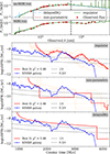 |
Fig. F.1. Best SEDs and corresponding sSFHs of the SIMBA galaxy. The top figure shows comparison of SEDs from the no-MIRI vs MIRI run. The observed fluxes, obtained by convolving filter with simulated SED, are marked with red circles. The colours and line styles of SEDs correspond to the used SFH. The dashed black line marks position of JWST/MIRI F560W filter. The bottom figure compares the sSFHs directly from SIMBA and from CIGALE from the MIRI run. From top to bottom: Regulator, non-parametric, and delayedBQ SFH. The blue line shows values of sSFH directly from SIMBA galaxy catalogue. The red line shows the best CIGALE fit. The orange lines in the background in regulator and non-parametric panels show the other four best fits (each probing 200 random models; see Sect. 3.2). The dashed and dotted lines show star-forming and quiescent threshold, respectively, proposed by Pacifici et al. (2016). |
Now, we focus only on MIRI run only. We report a fairly consistent M★ estimate. In all three runs the estimated mass was lower than the real one in SIMBA, by a factor of ∼2 (0.2 dex) for delayedBQ and by a factor of ∼3 (0.4 dex) for the non-parametric and regulator models. The estimated SFR in each run is around ∼10 M⊙/yr, which is ∼2-3 order of magnitude higher than the simulated value. While this is a large deviation, in each run the galaxy is considered quenched by every criterion, even the most conservative one. Finally, in SIMBA simulation, our galaxy formed at z > 7. However, in CIGALE runs the estimated formation redshift is ∼6, 4.5, and 4 for the delayedBQ, non-parametric and regulator models, respectively.
We then follow the method described in Appendix E to prepare sSFHs for each run (see Fig. F.1). We estimate the quenching moment τq and the quenching time Tq the same way as in the main text. The simulated galaxy has quenched at τq ∼ 3400 Myr, and the quenching lasted Tq ∼ 500 Myr. For CIGALE results, only the regulator SFH has a resolution sufficient to estimate these parameters. We use the five best fits (see Sect. 3.2) to calculate the standard deviation and use it as uncertainty. We report τq = 3880 ± 325 Myr and Tq = 425 ± 285 Myr. Thus, we find a similar trend to the observed galaxies. We can recover τq, which is directly related to the ΔT. It converges to the same value with low scatter, and we can use it as an evolutionary tracer. We can also recover the true value of Tq, but the scatter is large (∼67%). We should not use Tq based on only photometry studies.
Appendix G: QG control sample
As a sanity check, we compare our results to massive QGs found by Carnall et al. (2023a) and nine QGs from Long et al. (2024). In Carnall et al. (2023a) the authors found 15 sources using HST/NIRCam observations; however, the positions of only three of them were observed by MIRI (IDs from Table 2 in Carnall et al. 2023b: ID8888 with 10μm, 12.8μm, 15μm, and 18μm detections, ID29497 with 15μm detection, and ID17318 with 15μm upper limit). In Long et al. (2024) the authors found 44 QGCs using the empirical NIRCam colour-colour diagram. The position of only nine of them were observed by MIRI producing in total: three detections and one upper limit in 5.5μm, four detections and one upper limit in 7.7μm, two detections in 10, 12.8, and 18μm, and one detection and one upper limit in 15μm.
Firstly, the quiescent nature of all three sources from Carnall et al. (2023a) agrees within all three runs of the SFH model and in both the MIRI and no-MIRI runs according to the Koprowski et al. (2024) MS criterion. We do not recover only two to three QGs (depending on the SFH model) from Long et al. (2024). In total, we find 75-83% of the QGs in these two works.
Using the sSFR quiescence criterion, only the delayedBQ model classifies all three Carnall et al. (2023a) objects as QGs, while the regulator and non-parametric models find object 8888 not quiescent. Using the MIRI run, we recovered four to six out of nine QGs defined in the Long et al. (2024) sample, while with the no-MIRI run, this number drops to two to four. Thus, we find 50-75% of the QGs found in other works.
We report the M★ are in perfect agreement with previous studies, up to < 0.3 dex within all CIGALE runs. Finally, the inclusion of MIRI points strongly influences the AV for two Carnall et al. (2023a) galaxies; AV decreases by up to∼0.80 mag for galaxy ID29497 and by up to ∼0.4 mag for galaxy ID8888, depending on the SFH model. For galaxy ID17318 (with one upper limit), the inclusion of MIRI does not change the AV estimation significantly (the change is ±0.1 mag, depending on the SFH model).
Appendix H: Bin ranges
The bins and sub-bins ranges of M★ and ΔT are presented in Table H.1.
Summary of M★ and ΔT ranges of bins used for Fig.6.
All Tables
All Figures
|
Fig. 1. Exemplary QGCs from our final sample: Massive system on the left and a less massive one on the right. Top: CIGALE SEDs. Solid and dashed black lines show the best–fit SEDs for the same galaxy using the regulator SFH with and without JWST/MIRI photometry for the MIRI and no–MIRI runs, respectively. Blue circles are detections; triangles are 3σ upper limits. JWST cutouts are displayed above each SED. Shaded envelopes indicate the range of K–band–normalised SEDs for QGCs binned by median AV; the legend lists the median AV values and number of objects in each bin. Bottom: sSFHs for the same QGC from the MIRI run. The solid dark blue, dashed violet, and dash-dotted light blue lines correspond to the regulator, non-parametric, and delayedBQ models, respectively. The thick and thin dark-blue lines show the difference between MIRI and no-MIRI runs. The dotted black line marks the quiescent threshold and the dashed black line the star-forming threshold (following Pacifici et al. 2016). Arrows mark the quantities used in this work for the regulator model: the quenching time, Tq, the quenching moment, τq, the cosmic time at the observation redshift, τ(zo), and the time since quenching, ΔT ≡ τ(zo)−τq. |
| In the text | |
|
Fig. 2. Top: Distribution of the M★ in function of redshift of the final sample from the regulator MIRI run. Bottom: Distributions of differences in the main physical properties (SFR in M⊙/yr and the M★ in M⊙, AV in mag, age in Myr) between the MIRI and no-MIRI runs. The hatched region shows the 90th percentiles of the distributions (P90) in both directions. |
| In the text | |
|
Fig. 3. Difference in estimated physical properties of galaxies from the final sample using different SFH models within the MIRI run as a function of redshift. From left to right: DelayedBQ-non-parametric, non-parametric-regulator, and regulator-delayedBQ. From top to bottom: Distribution of difference for: AV in mag, age in Myr, SFR in M⊙/yr, and the M★ in M⊙. The dashed blue line presents the median of distribution. The hatched region shows the 90th percentiles of the distributions (P90) above and below the median value. |
| In the text | |
|
Fig. 4. Top: SFR-M★ plane for different redshifts with galaxies from the final sample from the MIRI run with the regulator SFH. The different lines present quiescence selection from the literature: the sSFR criterion in black; Popesso et al. (2023) in dark blue; Koprowski et al. (2024) in violet; and Mérida et al. (2026) in light blue. The grey crosses represent QGCs selected by the sSFR criterion in the regulator MIRI run, which were not recovered in the no-MIRI run. Bottom: Comparison of the QGCs sample size, depending on the selection criterion and SFH model for the MIRI and no-MIRI runs. The colours of the points represent the MSs and are the same as at top panel. The markers represent SFH model: Regulator (triangle); non-parametric (circles); and delayedBQ (squares). The dashed line shows one-to-one relation. With the shaded regions we mark 30%, 60%, and 100% relative distance from the one-to-one relation. |
| In the text | |
|
Fig. 5. Comparison of UVJ diagrams for galaxies with z < 2.5 (top six panels) and 2.5 ≤ z < 6 (bottom six panels) for mass-complete sample (M* ≥ 108 M⊙) from different runs. The squares are sized logarithmically according to the number of galaxies in the bin. We colour-coded the median attenuation in V-band (AV) as the histogram in the background. The grey crosses represent the QGCs selected with sSFR criterion. The dashed blue line shows the redshift-dependent criterion for quiescence by Antwi-Danso et al. (2023). We marked the fraction of QGCs (sSFR criterion) caught by UVJ criterion in the lower right corner of each panel. Top panels: Results from the MIRI run. Bottom panels: Results from the no-MIRI run. The columns are related to the SFH model used in the run, from left to right: DelayedBQ, non-parametric, and regulator. Additionally, we included galaxies we were able to recover as QGs using the Koprowski et al. (2024) MS offset criteria, with cyan crosses marking QGs from Carnall et al. (2023a) and magenta stars marking QGs from Long et al. (2024). For details, see Appendix G. |
| In the text | |
|
Fig. 6. Relation between time since quenching (ΔT) and the AV of the mass-complete QGCs at z ≤ 2.5. The columns show different SFH models used in the run, from left to right: DelayedBQ, non-parametric, and regulator, while the rows show the MIRI vs no-MIRI runs. The colours represent the median M★ of each bins. The arrows on the left of each panel show the weighted mean for the corresponding M★ bin. |
| In the text | |
|
Fig. A.1. Completeness analysis using the first method with the regulator MIRI run results. Top left: Apparent magnitude completeness curve. The red points are values from (Merlin et al. 2024), the blue line is the interpolated curve, and the dashed orange line is the value for 90% completeness. Top right: M★-redshift plane with histograms. In grey we mark galaxies below the mag90% limit, while the white to blue colours represent the apparent magnitude of each galaxy. The red lines show the 90% completeness for each redshift bin. Bottom panels: Histograms for each of the redshift bins. The estimated maximum of the distribution is shown with dashed red lines. The median redshift of the galaxies in bin is given a the top of each panel with the maximum of the distribution. |
| In the text | |
|
Fig. A.2. M★ as a function of maximum redshift for detection above 90% completeness. Top: Results for SFGs. Bottom: Results for QGs. The grey points are individual galaxies. The larger blue and red points present the largest M★ in each redshift bin. The solid blue and red lines show the linear fit, while the dashed orange line present the M★ at z = 6 according to the fit. |
| In the text | |
|
Fig. B.1. Completeness curves for MIRI observations from the CEERS program. Each panel represents different band, which is written in the upper-right corner. Each coloured line represents MIRI pointing. The dashed grey line marks completeness of 50%, and the circles show the estimated 5σ upper limit. |
| In the text | |
|
Fig. D.1. Photo−z estimation with and without MIRI data for galaxies with. The colour represent the stellar mass estimated in the run with MIRI data. The dashed magenta line shows 1:1 relation, while the solid black line represent the best fit. The grey shaded region show the non-outliers region defined as |zwithMIRI − zwithoutMIRI|/(1 + zwithMIRI) > 0.15. |
| In the text | |
|
Fig. F.1. Best SEDs and corresponding sSFHs of the SIMBA galaxy. The top figure shows comparison of SEDs from the no-MIRI vs MIRI run. The observed fluxes, obtained by convolving filter with simulated SED, are marked with red circles. The colours and line styles of SEDs correspond to the used SFH. The dashed black line marks position of JWST/MIRI F560W filter. The bottom figure compares the sSFHs directly from SIMBA and from CIGALE from the MIRI run. From top to bottom: Regulator, non-parametric, and delayedBQ SFH. The blue line shows values of sSFH directly from SIMBA galaxy catalogue. The red line shows the best CIGALE fit. The orange lines in the background in regulator and non-parametric panels show the other four best fits (each probing 200 random models; see Sect. 3.2). The dashed and dotted lines show star-forming and quiescent threshold, respectively, proposed by Pacifici et al. (2016). |
| In the text | |
Current usage metrics show cumulative count of Article Views (full-text article views including HTML views, PDF and ePub downloads, according to the available data) and Abstracts Views on Vision4Press platform.
Data correspond to usage on the plateform after 2015. The current usage metrics is available 48-96 hours after online publication and is updated daily on week days.
Initial download of the metrics may take a while.