| Issue |
A&A
Volume 708, April 2026
|
|
|---|---|---|
| Article Number | A44 | |
| Number of page(s) | 16 | |
| Section | Extragalactic astronomy | |
| DOI | https://doi.org/10.1051/0004-6361/202558108 | |
| Published online | 26 March 2026 | |
Constraints on dynamically formed massive black holes in little red dots from X-ray non-detections
1
Dipartimento di Fisica, Sapienza Università di Roma, Piazzale Aldo Moro 5, 00185 Rome, Italy
2
Physics Department, College of Science, United Arab Emirates University, PO Box 15551 Al-Ain, UAE
3
INFN – Sezione Roma1, Dipartimento di Fisica, Università di Roma La Sapienza, Piazzale Aldo Moro 2, I-00185 Roma, Italy
4
Sapienza School for Advanced Studies, Viale Regina Elena 291, I-00161 Roma, Italy
5
INAF – Osservatorio Astronomico di Roma, Via di Frascati 33, 00078 Monte Porzio Catone, Italy
6
Department of Physics, New York University Abu Dhabi, PO Box 129188 Abu Dhabi, UAE
7
Center for Astrophysics and Space Science (CASS), New York University Abu Dhabi, PO Box 129188 Abu Dhabi, UAE
8
Departamento de Astronomía, Universidad de Chile, Casilla 36-D, Santiago, Chile
9
Astronomisches Rechen-Institut, Zentrum für Astronomie, University of Heidelberg, Mönchhofstrasse 12-14, 69120 Heidelberg, Germany
★ Corresponding authors: This email address is being protected from spambots. You need JavaScript enabled to view it.
, This email address is being protected from spambots. You need JavaScript enabled to view it.
Received:
13
November
2025
Accepted:
23
February
2026
Abstract
The existence of extremely massive and compact galaxies, also called little red dots (LRDs), at z ≳ 2 challenges models of early structure formation, suggesting extremely rapid stellar and black hole (BH) assembly. These galaxies are efficient environments for rapid BH growth, but several LRDs show no evidence of strong emission from the active galactic nuclei in X-rays. Our work uses a subsample of X-ray non-detected LRDs to determine whether the collision-based BH formation scenario is compatible with the non-detections and to constrain the physical parameters (e.g., metallicity) and observational parameters (e.g., column density). Our results show that LRDs might be ideal birthplaces for the formation of massive BHs, particularly in the case of a mass-radius relation Rgal ∝ M0.6gal (similar to spiral galaxies in the local Universe). Given the high stellar densities, collision-based models suggest seed masses greater than those observed in the local Universe, and these are compatible with the mass-radius relation of high-redshift BHs. We modeled the BH seed formation and subsequent X-ray emission to investigate the physical and observational parameter space to compare with the observed X-ray upper limits in the soft (0.3 − 2 keV) and hard band (2 − 7 keV). We found that exponents in the mass-radius relation above 0.55 favor the collision-based scenario, but consistency with the stacked X-ray analysis requires specific combinations of accretion and obscuration parameters. Additionally, we found that constant or increasing star formation rate scenarios assuming high Eddington ratios and long duty cycles are feasible, but require higher column densities and/or a higher level of metal enrichment in the shielding columns. Alternatively, moderate sub-Eddington accretion rates seem to be sufficient to reconcile the massive seeds with their final observed masses, consistent with the observed X-ray weakness. Overall, we conclude that even if LRDs were initially starburst galaxies, they should evolve into an active galactic nucleus.
Key words: galaxies: evolution / galaxies: formation / galaxies: high-redshift / galaxies: nuclei / quasars: supermassive black holes / X-rays: galaxies
© The Authors 2026
 Open Access article, published by EDP Sciences, under the terms of the Creative Commons Attribution License (https://creativecommons.org/licenses/by/4.0), which permits unrestricted use, distribution, and reproduction in any medium, provided the original work is properly cited.
This article is published in open access under the Subscribe to Open model. This email address is being protected from spambots. You need JavaScript enabled to view it. to support open access publication.
1. Introduction
The detection of extremely compact and massive galaxies at high-redshift by JWST challenges the current knowledge of galaxy formation and evolution. The masses of these galaxies, the so-called little red dots (LRDs), range between 108 and 1012 M⊙ in an effective radius of 3 − 300 pc (e.g., Matthee et al. 2024; Greene et al. 2024; Akins et al. 2025). An LRD is characterized by its V-shaped spectral energy distribution (SED), which features an inclined red continuum in the optical rest frame together with a blue UV counterpart in the rest frame (Kocevski et al. 2023; Akins et al. 2023; Maiolino et al. 2024). The high sensitivity of JWST surveys, particularly the JWST Advanced Deep Extragalactic Survey (JADES; Eisenstein et al. 2025, 2026), facilitates the discovery and characterization of LRDs over the GOODS-South and GOODS-North fields, contributing to the measurement of their properties (e.g., Rinaldi et al. 2025). However, the origin of this peculiar spectrum is still strongly debated. The slopes in the optical band are consistent with (i) emission from dusty star formation (i.e., emission dominated by young stellar populations; Williams et al. 2024; Pérez-González et al. 2024) or (ii) reddened active galactic nuclei (AGNs), in which thermal emission from the accretion disk dominates on scales smaller than 1 pc with temperatures higher than 105 K (Labbe et al. 2025; Matthee et al. 2024). Similarly, the excess of UV emission might be explained by light from the central AGN and stellar emission emerging from a relatively dust-free host or by light escaping without attenuation due to patchy dust, as observed in some lower-redshift dusty star-forming galaxies (e.g., Casey et al. 2014) and red quasars (Glikman et al. 2023).
While the broad emission lines (full width at half maximum of ∼2000 km s−1) observed in many LRDs suggest the presence of accreting supermassive black holes (SMBHs) with masses of at least 107 − 108 M⊙ (Matthee et al. 2024), confirming this AGN nature in the X-ray regime has proven difficult. Recent stacking analyses of X-ray non-detected sources have yielded strict upper limits. For instance, Sacchi & Bogdán (2025, hereafter S+25) constrained the emission of galaxies lacking individual X-ray detections. The upper limits they found are incompatible with unobscured super-Eddington accretion models. Their results imply that if massive black holes (BHs) are present, they must be either significantly less massive than optical estimates suggest or are buried under extreme column densities (NH ≳ 1025 cm−2). This characteristic X-ray weakness is supported by independent studies. Ananna et al. (2024) found no significant detection in a stack of 21 high-redshift LRDs, placing upper limits on BH masses of ≲(1.5 − 16)×106 M⊙ assuming Eddington-limited accretion. Similarly, Yue et al. (2024) reported only tentative detections in a stack of 34 LRDs, suggesting that any central engine must be intrinsically weak or heavily obscured. This discrepancy between the optical evidence for massive BHs and the general lack of strong X-ray emission presents a major open question regarding the nature and growth of LRDs.
Despite these observational puzzles, the structural properties of LRDs make them unique laboratories for BH formation. On average, LRDs have high stellar masses (Mgal) of a few 1010 M⊙ within radii of Rgal ∼ 135 pc at z ∼ 7 − 9 (Baggen et al. 2023), with some systems being even more compact (Rgal < 35 pc, Furtak et al. 2023). The mean density in the core of LRDs is ∼104 M⊙ pc−3, with the highest core densities reaching 108 M⊙ pc−3 (Guia et al. 2024). Theoretical models predict that in environments exceeding 107 M⊙ pc−3, runaway stellar collisions become inevitable. Numerical simulations show that stellar mergers can produce a single supermassive star, which then collapses directly into an intermediate-mass BH (Fujii et al. 2024). Other pathways include the growth of a massive star within a dense cluster formed from a fragmented gas cloud (Tagawa et al. 2020). Recent N-body models further support this scenario, showing that collisions in dense clusters can efficiently produce intermediate-mass BHs (Vergara et al. 2023, 2024, 2025, 2026, hereafter V+). Semi-analytic models of nuclear star clusters (NSCs) indeed suggest that this collision-based channel likely makes a relevant contribution to the total population of SMBHs (Liempi et al. 2025).
We aim to constrain the properties of massive BHs formed via stellar collisions in LRDs by exploiting the reported limits on their X-ray emission. We construct a dynamical evolution model for LRDs to predict the mass of collisionally formed seeds and their subsequent X-ray signatures. By comparing these predictions with the stacking limits from S+25, we identify the regions of parameter space, specifically regarding the galaxy mass-radius relation and BH accretion duty cycles, that are consistent with the current non-detections.
This work is organized in the following sections: In Sect. 2.1 we briefly describe the data collection of our sample. The model for the temporal evolution of LRDs is described in Sect. 2.2. We describe the results we obtained in Sect. 3 and discuss them in Sect. 4.
2. Data and general framework
In this section, we introduce the observational data employed for our data analysis. Subsequently, we introduce a simplified dynamical model for the evolution of LRDs. We estimate the masses of SMBHs that might form in these dense systems. Finally, we discuss the observational constraints from the X-ray background and our emission model for estimating the expected X-ray emission from the BH population.
2.1. Population data
We used a subsample of 55 galaxies selected by S+25 from the parent sample of Kocevski et al. (2025). We considered the galaxies for which deep Chandra data have been available without individual X-ray detections. The authors (S+25) employed the stacking technique to combine the data from the different sources and derive an upper limit on the X-ray flux that may come from this population. The parent sample contains the photometric redshift and the absolute magnitude in the UV band (MUV) of 341 LRDs spanning the redshift range z ∼ 2 − 11 using data from the Cosmic Evolution Early Release Science (CEERS) survey, the Public Release IMaging for Extragalactic Research (PRIMER), the JWST Advanced Deep Extragalactic Survey (JADES), the Ultradeep Nirspec and NIRCam Observations before the Epoch of Reionization (UNCOVER), and the Next Generation Deep Extragalactic Exploratory Public (NGDEEP) survey. In contrast, the subsample of S+25 contains galaxies in the JADES and NGDEEP surveys, which do not have X-ray detections in a similar redshift range z ∼ 3 − 11.
As input for our dynamical model, we estimated the stellar mass (Mgal) for our galaxies using the MUV − Mgal correlation (e.g., González et al. 2011; Duncan et al. 2014) at different redshifts. Specifically, it is well known that Mgal is correlated with the UV absolute magnitude MUV as
 (1)
(1)
where a, b are free parameters that depend on the redshift. In Table 1 we list the values adopted for the free parameters in Eq. (1). In Fig. 1 we show the comparison between the resulting stellar masses and the masses reported in the sample of Akins et al. (2025, hereafter A+24). We find a good agreement regarding the overall mass range, while we note that the redshift distribution in the subsample of S+25 is slightly different, extending to somewhat lower (z ∼ 2.8) and also somewhat higher (z ∼ 11) redshifts than the sample of A+24.
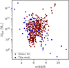 |
Fig. 1. Galaxy stellar masses obtained for the subsample of S+25 using the previous observed scaling correlation between MUV and Mgal (Eq. 1) compared to the stellar masses of the galaxies in the sample of A+24, both shown as a function of redshift. |
As the radii for the sources found in the sample of S+25 have not been yet published, we assumed that they follow the same distribution as those of the sample of A+24, where it appears roughly independent of mass (see Appendix A). We obtained the effective radius of the galaxies in the sample of A+24. The authors multiplied the radius (in mas) by the angular distance DA(z). As galaxy sizes span several orders of magnitude, we performed the fitting in logarithmic space, defined as x = log10(Rgal/pc). We employed a Gaussian mixture model approach, where the distribution is described as the sum of K independent Gaussian components. The probability density P(x) is given by  where wk, μk, and σk are the weight, mean, and standard deviation of the kth component, respectively, subject to the constraint ∑wk = 1. The parameters were estimated using the expectation-maximization algorithm. We compared models with K = 1 and K = 2 components (see Fig. 2), evaluating the goodness-of-fit using the reduced chi-squared statistic (χν2) calculated over the histogram bins assuming a fixed size equal to 0.2 dex. Prior to fitting, we excluded a single object with an effective radius Reff > 1 kpc. As this object was the sole galaxy in the sample with such a large extent, treating it as part of the continuous distribution would disproportionately affect the parametric fit or require a statistically unjustified third component; removing it allowed us to robustly characterize the primary compact and extended populations. Even though the redshift and the mass distributions of the sample of A+24 and the subsample of S+25 are slightly different, we assumed that the radius distribution used here provides a conservative estimate, as discussed in Appendix B. We determined the effect on the results by sampling from the one- and two-component distributions, but found no relevant changes.
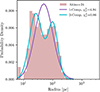 |
Fig. 2. Probability density distribution of effective radii (Rgal) for the galaxy sample from A+24. The shaded red histogram shows the observed data binned in logarithmic intervals. The solid curves represent the best-fit Gaussian mixture models, assuming a single component (purple) and two components (cyan). We show the reduced chi-squared (χν2) for each model. |
The cosmological parameters adopted for all calculations corresponds to the Planck Collaboration VI (2020) results, with H0 = 67.66 km s−1 Mpc−1, Ωm, 0 = 0.31. All magnitudes are in the AB system (Oke 1974), as in A+24.
2.2. Dynamics of little red dots
In this subsection, we describe our prescription for the mass and size evolution of LRDs. We employed a simplified toy model for the evolution of the mass and the radius of the LRD, in which the parameters Mgal and Rgal were approximated as power laws of time. Specifically, the evolution of the mass is given by
 (2)
(2)
with α = [0.1, 3] the exponent of the power law. On the other hand, the evolution of the radius depends implicitly on time. It assumes a correlation between the stellar mass and the radius, that is,
 (3)
(3)
where β is the exponent of the correlation Rgal − Mgal1 and is assumed to be in the range of 0.1 − 1.5. This parameter is a key point of observational debate at high redshift. For example, Allen et al. (2025) measured a constant size-mass relation slope of β ≈ 0.215 for star-forming galaxies from z = 3 − 9. In contrast, Ormerod et al. (2024) found that this relation breaks down at z > 3, with galaxy sizes showing little to no dependence on stellar mass (implying β ≈ 0). For NSCs, we have β ∼ 0.5, while early-type galaxies have typical values of β = 0.55 − 0.6 (Shen et al. 2003) and late-type galaxies have β = 0.22 − 0.27 (Shen et al. 2003; Lange et al. 2015). Our model tests a wide range of β and can therefore provide constraints on which evolutionary track is more consistent with the observed properties of LRDs.
2.3. Black hole formation via stellar collisions
Escala (2021) provided observational evidence that supported the formation of a massive BH through stellar runaway collisions in dense stellar systems. In systems with collisional timescales (tcoll) shorter than the age of the system, a global instability leads to massive object formation via runaway stellar collisions. This scenario was tested with dedicated N-body direct simulations by V+23 as well as through a detailed comparison and analysis with literature data (V+24; V+25a; V+25b).
In Fig. 3 we show a mass-radius diagram divided into two main regions by the condition of the collisional timescale (solid black line, defined in Eq. 4) being equal to the age of the Universe (tcoll = 13.7 Gyr). On the left side of the collisional timescale, collisions are relevant. The collision timescale there is shorter than the age of the system (i.e., tcoll ≤ tH), with tH the age of the system. On the right side of the collisional timescale line, collisions are less relevant (but still occur) as the collision timescale exceeds the age of the system (tH < tcoll). We show that the observed NSCs reside in a stable regions within the mass-radius diagram of stellar systems, delimited by a line for which the collision timescale tcoll becomes 13.7 Gyr. We define it as (Binney et al. 2009)
 (4)
(4)
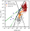 |
Fig. 3. Mass-radius diagram for stellar systems to illustrate relevant timescales and the position of different sources in different parts of the parameter space. The red dots show LRDs from A+24, gray dots show NSCs in the local Universe (Georgiev et al. 2016; Neumayer et al. 2020), blue dots show well-resolved BHs, and orange dots show spatially unresolved BHs (Gültekin et al. 2009; Escala 2021). The solid black line represents the collisional timescale tcoll = 13.7 Gyr, and the dashed black line shows the relaxation time for trelax = 13.7 Gyr. We include (in green) a fiducial galaxy with mass 1010 M⊙ and radius 20 pc to show its trajectory in the mass-radius plane for β = 1 and 0.5, as defined in Eq. (3). The time evolution of the green line is from left to right. |
with n = ηMgal/(Rgal3M⊙) the number density of stars (η = 3/4π for systems with spherical symmetry),  the cross section, and Θ = 9.54[(M★ R⊙)/(R★ M⊙)](100 km s−1/σ)2 the Safronov number, and
  , which is the velocity dispersion under the assumption of virial equilibrium.
In Fig. 3 we also show the mass and radius (estimated as = 0.5dresol, with dresol the spatial resolution) of SMBHs in the sample of Gültekin et al. (2009), where we refer as well-resolved SMBHs to candidates with an influence radius (Rinf) larger than three spatial resolutions. These well-resolved BHs are located in the regime in which stellar collisions are relevant for the dynamics of the system. Spatially unresolved SMBHs (defined as Rind < 3dresol) are in the stable area. In these case, the radius should be regarded only as an upper limit. This does not represent an issue because a better resolution might shift the positions of the unresolved population to the left.
Similarly, LRDs are close to the regime in which collisions will be relevant, but in a different position on the mass-radius diagram. We include a fiducial galaxy in green (with a final mass equal to 1010 M⊙ and a radius of 20 pc) to show how it moves in the diagram (from left to right) as it evolves according to the power-law model (Eqs. 2 and 3) and reaches a final density ∼107 M⊙ pc−3 (assuming a system composed by solar-mass stars) similar to the LRD densities calculated by Guia et al. (2024).
As described in the introduction, LRDs are potential birthplaces for massive BHs because their cores can reach high densities (Guia et al. 2024). Different approaches (e.g., analytical, N-Body, and Fokker-Plank models Pacucci et al. 2025) showed that the formation of a massive object through pure stellar dynamics is expected, and that a massive object most probably formed directly in the supermassive range in the case of LRDs, which were initially even more compact (Escala et al. 2025).
In direct N-body simulations investigating this scenario, it was found that the BH formation efficiency, defined as ϵBH = (1+Mstellar/MBH)−1 (where Mstellar is the stellar mass of the system and MBH is the mass of the BH), reached values up to ∼50% in dense clusters with stellar masses of ∼104 M⊙ (V+23). This efficiency represents a saturation limit that is observed in environments with densities of ∼107 M⊙ pc−3. Such extreme conditions are consistent with the estimated core densities of LRDs (Guia et al. 2024). Furthermore, comparisons with observations of dense stellar systems suggest that this mechanism can account for BHs with masses up to ∼107 M⊙ (V+24), supporting the scenario in which the dense cores of LRDs are efficiently converted into massive BHs and further showed that this efficiency depends on the ratio of the stellar mass to the critical mass Mcrit(R), which encapsulates the idea of stellar collisions, defined as
 (5)
(5)
where R is the radius of the system, M★ the mass of a single star, tH the age of the system, and Σ0 the effective cross section. In our model, we employed the fit formula from V+25b to estimate the efficiency of the forming BH, given as
![Mathematical equation: $$ \begin{aligned} \epsilon _{\rm BH} \left( \frac{M_{\rm gal}}{M_{\rm crit}} \right)= \left[ 1+\exp \left(-4.63\left[\log \left(\frac{M_{\rm gal}}{M_{\rm crit}}\right)-4\right]\right)\right]^{-0.1}. \end{aligned} $$](/articles/aa/full_html/2026/04/aa58108-25/aa58108-25-eq26.gif) (6)
(6)
In galaxies that meet this condition, we evaluated this efficiency when t = tcoll because the value of the efficiency is highest at that time. Even when the condition is not fulfilled, efficiencies higher than unity are still possible, implying that a relevant fraction of the stellar mass goes into a massive object. We verified that the product ϵBHMgal monotonically increases with time in these models. Therefore, we evaluated the efficiency at the observed age of the galaxy when t = tage, where we estimated the age of the system based on its observed redshift. In summary, we assigned the BH mass as MBH = ϵBHMgal, where the efficiency is given by Eq. (6). The ratio of the galaxy mass and the critical mass (Mgal/Mcrit) was accordingly evaluated at t = tcoll or t = tage. The maximum BH masses for which the models were validated were about 107 M⊙, which we took as an upper limit (V+23; V+24). While the limit of validity of the model might extend to higher masses, we nonetheless note that additional effects might become relevant. Stellar evolution is uncertain at these mass scales and for these wide dynamical ranges. We adopted this upper limit because the observational samples in the above studies still included 107 M⊙ BHs for which the relation was found to be valid. Nonetheless, the exact validity limit needs to be further established through theoretical and observational investigations.
The implications of these high formation efficiencies (ϵBH ∼ 50%) first suggest that in the densest high-redshift environments, the central BH is not merely a byproduct of galaxy evolution, but a dominant structural component. This might explain the anomalously high MBH/Mgal ratios observed in LRDs (Juodžbalis et al. 2024). Second, this scenario alleviates the need for continuous super-Eddington accretion to grow the BH from stellar mass. Consequently, these massive BHs can exist in a quiescent or low-accretion state, which naturally reconciles their high inferred masses with the strict X-ray non-detections reported in stacking analyses.
2.4. X-ray background data and black hole emission
We collected the X-ray data from the stacking procedure by S+25. The authors employed data from the Chandra Deep Field South (CDF-S). The total exposure time, using the data from all of the available sources, amounts to ≈400 Ms, leading to an unprecedented sensitivity of ∼4 × 10⁻¹⁸ erg s−1 cm−2.
The upper limits of the detections are provided at the 3σ level, where σ represents the standard deviation of the background noise. For the soft (0.3 − 2 keV) and the hard band (2 − 7 keV), the upper limits are < 4.7 × 10⁻¹⁸ and < 1.3 × 10⁻¹⁷, respectively, in units of erg s−1 cm−2.
We modeled the intrinsic X-ray emission of the SMBHs formed in our model. We assumed a power law with a high-energy exponential cutoff (e.g., Yang et al. 2020),
 (7)
(7)
where Γ is the photon index. The value of Γ is usually set at ≈1.8 − 1.9 (e.g., Piconcelli et al. 2005; Yang et al. 2016; Liu et al. 2017; Yang et al. 2020), and Ecut = 300 keV for Seyfert galaxies (see Ricci et al. 2017). However, the weak emission of LRDs in the X-ray band is consistent with a steeper value of Γ ≈ 2.4 ± 0.1 (e.g., Zappacosta et al. 2023) or with a very low-energy cutoff Ecut ≈ 20 keV. We adopted the canonical value Γ = 1.9 with a low-energy cutoff of Ecut = 20 keV. We also checked the possibility of Γ = 2.4, but found no difference in our results.
The normalization constant of Eq. (7) was set such that the integrated X-ray luminosity corresponded to a fraction of the Eddington luminosity of the BHs, that is,
 (8)
(8)
where Uduty is the duty cycle, ϵEdd is ratio of the bolometric to the Eddington luminosity (LEdd = 1.26 × 1038(MBH/M⊙) erg s−1), ϵX is the fraction of the bolometric luminosity emitted in X-rays, and finally,  is a factor that considers the possibility that not all the galaxies form a BH.
Our approach constrains the product  and not individual parameters. It ranges over 0 < k ≤ 0.3. Here, 0 is the lower limit of no emission. The upper bound corresponds to a quasar growth scenario that is necessary to grow massive BHs at z > 5, implying, for example, a near-unity occupation fraction with an active duty cycle of 100% at ϵEdd = 0.3, or alternatively, short bursts of super-Eddington accretion (ϵEdd ∼ 1) with a duty cycle of 30%. The conversion to observable X-ray flux is then modulated by ϵX, which we adopted from luminosity-dependent bolometric corrections (BCs; Duras et al. 2020) to account for the spectral softening at these high accretion rates.
As the parameter k in our model represents the effective time-averaged accretion activity, this physically degenerates the Eddington ratio (ϵEdd) and the accretion duty cycle (Uduty), such that k ∝ ϵEdd × Uduty. For an X-ray stacking analysis, which averages the flux over the population, these two factors are often indistinguishable; a source accreting continuously at 1% Eddington luminosity produces a stacked signal that is similar to that of a source accreting at 100% Eddington luminosity with a 1% duty cycle. However, the duty cycle has important implications for the mass growth. To grow from a small seed to 108 M⊙, a BH requires not just a high accretion rate, but also a high duty cycle (Uduty ∼ 1).
We included an absorption model to take the attenuation of the emission due to the column densities into account, which we described via a suppression factor, that is, exp(−σtot(E)Nave), where σtot(E) is the total cross section as a function of the energy of photons (see Eq. 9) and Nave is the average column density. The total cross section is given by
 (9)
(9)
with Z the metallicity, and A⊙i are the solar abundances taken from Wilms et al. (2000). The cross sections for the metals (σi(E)) were obtained using the fits provided by Verner et al. (1996). Finally, the observed flux in a certain band is given by
 (10)
(10)
where DL(z) is the cosmological luminosity distance, the factor (1 + z) corrects the flux for the redshifting of the photons, and the energy interval is stretched by cosmic expansion.
3. Results
We describe the main results of our work. In Sect. 3.1 we show the results for the expected BH population based on the collision-based formation scenario. Subsequently, we provide the constraints on this population from the upper limits on the X-ray flux in Sect. 3.2. For all the calculations, we adopted the conservative scenario, in which BH masses cannot exceed 107 M⊙, as described in Sect. 2.3.
3.1. Expected black hole population from the collision-based scenario
We briefly recall here that for galaxies that reach the condition t = tcoll during their mass (size) evolution, we calculated the expected mass of the SMBH at that time; when this was not the case, we calculated the product ϵBHMgal at the time corresponding to the age of the stellar system, as defined via the observed redshift. We first determined for how many systems the condition t = tcoll was fulfilled and assigned them the parameters α and β, which are the power-law exponents that describe the time evolution of the mass of the LRDs and their adopted mass-radius relation. In Fig. 4 we provide a color-coded map of the fraction fcoll of systems that reached this condition as a function of the parameters α and β. We note that the results predominantly depend on the β parameter. We obtained high fractions of such galaxies using β ≳ 0.7, even though in some cases, the condition is still reached for β ∼ 0.5 (adopting α ≳ 1). Here, α = 1 corresponds to a constant star formation rate (SFR), while α ≳ 1 indicates an increasing SFR with time. The constraints on β are somewhat more difficult to reconcile; in observed NSCs, we obtain a typical relation with β ∼ 0.5. For early-type galaxies, typical values are β = 0.55 − 0.6 (Shen et al. 2003), while for late-type galaxies, typical values are β = 0.22 − 0.27 (Shen et al. 2003; Lange et al. 2015). If the mass-radius relation of LRDs is somewhat similar to spirals or NSCs and the SFR increases with time, it is thus conceivable that the condition t = tcoll will be reached at least in some systems, allowing for particularly high efficiencies of SMBH formation. If this condition is still not reached, a BH might still form, but perhaps with an efficiency on the percent level or lower than ∼1%, given through Eq. (6).
 |
Fig. 4. Fraction of galaxies in which BH formation is driven by the condition t = tcoll as a function of the power-law exponents α and β . The x-axis represents the exponent in the mass-radius relation |

In Fig. 5 we show the SFR according to our model for the galaxies in our sample for different values of α. Specifically, we show the distribution for α = 0.3, 1.0, and 2.9. For comparison, we include observational SFR estimations, in cyan we show the area corresponding to the SFR of a LRD at z ∼ 4.53, the lower limit of the SFR is obtained from the [OII] line corrected by AV = 0.9 ± 0.4 with a mean value of 22 ± 13 M⊙ yr−1, and the Hα (narrow) line (also corrected by AV = 0.9 ± 0.4) provides a slightly higher value of  M⊙ yr−1. However, the intrinsic luminosity at L1500, UV at 1500 Å from the UV continuum power-law fit suggest an SFR of 12 ± 0.3 M⊙ yr−1 (Killi et al. 2024). In violet, it is shown the SFR of three LRDs. The averaged SFRs (taking into account the last ∼100 Myr) are
  ,
,  , and
, and  M⊙ yr−1 (Wang et al. 2024). In gray, we show a LRD with the highest SFR estimated, the galaxy is observed at z = 4.47, and its SED suggests that stars dominate the continuum, which self-consistently explains the lack of an X-ray detection and the lack of a hot dust upturn in the mid-infrared. The main issue arises for the Hα luminosity. An SFR of 500 − 1000 M⊙ yr−1 is required to produce sufficient ionizing photons for this emission (Labbe et al. 2024). As expected, higher values of α (defined in Eq. 2) shift the distribution to the right. The peak of the distribution for α = 1.0 and 2.9 is consistent overall with the estimated SFRs from the literature. When we combine the information from Figs. 4 and 5 and confirm from observations that LRDs are compact and massive stellar systems that build in a short period of time, LRDs are more likely perfect places for the formation of massive BHs as result of stellar collisions.
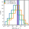 |
Fig. 5. Distribution of the SFR of our galaxy sample as function of α. We show the distribution for α = 0.3 (blue), 1.0 (green), and 2.9 (orange). The cyan area shows the SFR range for the J0647_1045 galaxy at z ∼ 4.53 (Killi et al. 2024), the violet area shows the range of three LRDs at z ∼ 7 − 8 (Wang et al. 2024), and in gray, we show an extreme case of an LRD at z ∼ 4.47 with a high SFR (Labbe et al. 2024). |
We now show the expected relation between the BH mass and galaxies in the framework of our models, in Fig. 6. There, we indicate the range of the possible solutions for α between 0.1 and 3 and β between 0.1 and 1.5. We highlight the results of a favorable case with α = 1 and β = 0.6, for which the efficiencies of forming massive BHs are rather high, and SMBHs tend to be produced well above the observed relation for local Universe galaxies. Our conservative scenario, in which the maximum allowed BH mass is 107 M⊙, as explained in Sect. 2.3 (yellow points), exhibits masses that scale with MBH/Mgal ≈ 0.1 for galaxies with masses up to 108 M⊙, while the local correlation measured by Reines & Volonteri (2015) scales as MBH/Mgal ≲ 0.001 (see the gray region in Fig. 6). Our optimistic scenario is shown in Fig. 6 (green dots), where all the BH seeds follow the MBH/Mgal ≈ 0.1 relation. It is expected that the model for α = 1.0 and β = 0.6 scales as MBH/Mgal ≈ 0.1. In this model, Mgal/Mcrit ∼ 10−2 − 10−1, implying BH efficiencies of about ϵBH ∼ 6 × 10⁻² − 10−1, which results in MBH ∼ 6 × 10⁻² − 10−1Mgal. We use the conservative scenario for the subsequent analysis. The masses obtained in this scenario are comparable with the high-redshift data points from Harikane et al. (2023), Maiolino et al. (2024), and Zhang et al. (2025). Nonetheless, as indicated in the figure, the overall possible parameter space is much larger, and depending on the assumed history of the galaxy, the parameter space also includes possible solutions with SMBHs at much lower masses. It is important to stress that the predictions provided here are only based on the seeding model itself and do not yet take possible growth via accretion of even super-Eddington accretion scenarios into account.
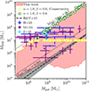 |
Fig. 6. MBH − Mgal relation from this work compared with observational results. All masses are given in solar masses (M⊙). The filled red area represents the parameter space spanned by the BH and host galaxy masses from this work for different combinations of α and β. In yellow we show the BH (and host galaxy) mass for α = 1.0 and β = 0.6 with a maximum mass seed of 107 M⊙. On the other hand, in green we show the masses without limiting the mass of the seed. The dashed black line and gray shaded area show the empirical MBH − Mgal relation for local (z = 0) galaxies (Reines & Volonteri 2015). We include data points from high-redshift (z = 4–7) observational studies from Harikane et al. (2023, blue open diamonds), data points from Maiolino et al. (2024, purple open squares), and from Zhang et al. (2025, cyan square). The dotted black lines indicate constant BH-to-galaxy mass ratios, labeled MBH/Mgal = 0.1 and 0.001. |
Based on the points above, we constrained α ≳ 1 from the comparison of the model histories with the typical SFRs (Killi et al. 2024; Wang et al. 2024; Labbe et al. 2024). To also have efficient collisions, β should be about 0.55. For a too low value of β, there would not be collisions, while a very high value is perhaps implausible as the largest observed mass-radius relations have power-law indices of 0.6 (Shen et al. 2003). When considering the X-ray constraints on our sources, we therefore used the above as the reference parameters for the dynamical model.
In Appendix C we show that subsequent accretion further affects these final BH masses. We demonstrate that for models in which seeds form early (e.g., tform ≈ 0.1 tage for high β), a long timescale is available for the mass growth (see Fig. C.1). Given the already high masses of our seeds, this subsequent growth must be constrained. In Fig. C.2 we explore the parameter space of the accretion by considering a low radiative efficiency BH model and a high-efficiency (rapidly spinning) model (e.g., Shapiro 2005). For low radiative efficiency BHs, even moderate sub-Eddington rates (L/LEdd ∼ 0.1) can lead to unphysically high final masses that systematically overshoot the observed relations. In contrast, for high radiative efficiency BHs, the mass growth is far more gradual and self-regulated. In this scenario, a moderate sub-Eddington rate (L/LEdd ∼ 0.1 as observed in Type 1 AGNs in the COSMOS field, Trump et al. 2009) is a physically plausible mechanism, producing a typical growth factor of ∼10. A low sub-Eddington rate (i.e., L/LEdd ≲ 0.01) is also entirely viable, representing the regime for low-luminosity AGNs (e.g., Ho 2008). While at least for the typical population, the X-ray constraints seem to limit these scenarios, we also emphasize that JWST has found a few objects with BH-to-bulge mass ratios of about 40% (Juodžbalis et al. 2024), which might be explained in a scenario of massive seed formation and subsequent efficient accretion.
3.2. X-ray background prediction
In this section, we present the resulting constraints from the comparison of the predicted emission in different scenarios with the observational constraints in the soft and hard X-ray bands. In the following subsections, we discuss the constraints that can be derived on the α and β parameters characterizing the history of the LRDs and their mass-radius relation, the average column density (Nave), metallicity (Z), and the k parameter defined in Eq. (8). As it is a large parameter space, it is clear that there are degeneracies in the possible constraints. Nonetheless, the upper limits on the fluxes rule out some possibilities, and with increasing information about these sources, perhaps more constraints can be tightened in the future.
3.2.1. Constraints on the star formation history and mass-radius relation
Already in Sect. 3.1, we constrained the possible parameter space for α and β considering the typical observed SFRs in LRDs and the model constraints from the requirement of having collisions. We determined whether these are also compatible with the constraints from the X-ray background. For this purpose, it is important to consider the parameters that can be assumed for the column density, metallicity, and activity level.
Observations by JWST have detected broad emission lines in the rest-frame UV/optical in principle, suggesting that broad-line regions are relatively unobscured (Greene et al. 2024). However, Maiolino et al. (2025) have argued that the dense dust-free clouds that cause the broad-line emission might simultaneously provide shielding in the X-rays. As a result, we either have the case of a very strong shielding (for which we are essentially unable to constrain the other parameters), or we are in the regime of low column densities. We focused on the second regime and adopted a reference value of Nave = 1021 cm−2 (we checked that the following results also hold for lower column densities). Measurements of the metallicity are not available so far, but we adopted a reference value of 0.01 Z⊙ as a typical value for high-redshift galaxies (e.g., Curti et al. 2024; Meyer et al. 2024; Sanders et al. 2024). In the regime of reasonably high metallicities, the product of the column density and metallicity has the main effect on the shielding because the dependence is exponential. The dependence on the activity parameter k, on the other hand, is only linear. Therefore, the activity parameter will be harder to constrain, but we assumed a typical value of k = 2.5 × 10⁻³ for definiteness. We explore variations in all these parameters in the following subsections.
The results for the soft and hard band are provided in Fig. 7 (panels a and b, respectively), where the color scale indicates the ratio of predicted versus observed flux as a function of α and β. The allowed parameter space for which the ratio of the predicted versus observed flux is lower than one (the red line shows where the ratio is equal to one) corresponds to the allowed region in the parameter space for the given choice of column, metallicity, and k-parameter. The X-ray constraints indicate the allowed parameter space for α and β, implying again α ≳ 1 and β < 0.6. The X-ray constraints are thus compatible with the requirements of the model. In the following subsections, we employ the constraints on α and β derived here, still under the assumption that obscuration is not relevant (as clearly no constraints could be obtained in a heavily obscured regime).
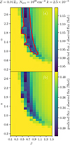 |
Fig. 7. Panel (a): Soft X-ray band (0.3 − 2 keV). Panel (b): Hard X-ray band (2 − 7 keV). The color bar shows the ratio of the predicted and observed flux for the soft and hard bands. The allowed parameter space for α and β is the region where the ratio of the predicted flux to the observed flux is lower than 1, which satisfies the soft X-ray and hard X-ray observational constraints, respectively. The red line represents ratio of the predicted and observed flux equal to one. |
The qualitative behavior of the hard band is very similar to that of the soft band. This is a generic result that the constraints obtained from the soft band are tighter, and we therefore mostly focused on these, similarly to Yue et al. (2024), who showed that the soft band is more sensitive to variations in column density, for example, than the hard band.
3.2.2. Metallicity and average column density
The amount of shielding of galaxies is an important parameter as the absorption of the X-ray flux can significantly tight possible constraints. It depends on the average column density in the sources, but also on the metallicity, as the cross section for X-rays can be significantly increased in the presence of heavy elements. We again considered our reference model for the collision-based BH formation scenario with α = 1 and β = 0.6 (considering that collisions must be sufficiently effective while still maintaining a realistic value of β) to assess the predicted flux and how it compares to the upper bounds.
In Fig. 8 we present the results for a value of k = 0.3, corresponding to a case with a high Eddington ratio, duty cycle, and BH population fraction in the top panel, and we show the results of a value equal to k = 2 × 10⁻³ for a more conservative scenario (bottom panel). The color bar indicates the ratio of predicted versus observed flux in the soft band. So far, no metallicities of LRDs have been inferred from observations. Furthermore, observations at low and high redshift suggest that the range of metallicities is not constrained by redshift. At high-redshift, highly evolved objects such as AGNs also show almost solar metallicities (e.g., Nagao et al. 2006).
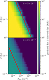 |
Fig. 8. Ratio of the predicted flux from our BH population and the observed limits in the soft band (0.3–2 keV; shown by the color bar). The solid red line denotes the curve where the ratio of the predicted and observed flux is equal to one. The y-axis shows the metallicities from solar to Z = 0.01 Z⊙. The x-axis is the average column density Nave in units of cm−2. We adopted k = 0.3 as an example of an extreme case of high activity (top panel) and a more conservative value k = 2 × 10⁻³ (bottom panel). |
For the high-activity model (top panel), the constraints correspond to a triangular shape, where column densities of ∼2 × 1021 cm−2 are required at low metallicities, while with increasing metallicity, even lower columns of ∼2 × 1019 cm−2 can be sufficient. We verified that the corresponding results for the hard band are very similar. At a lower value of k, the constraints become tighter and the required column density for shielding decreases compared to the previous result. A column density of ∼9 × 1019 cm−2 is required to shield the emission at Z = 10−2 Z⊙. On the other hand, at solar metallicities, the required density is ∼3 × 1018 cm−2.
We note that in the high-activity regime (k = 0.3), we recovered tighter constraints than in the conservative scenario (k = 2 × 10⁻³). This may appear counter-intuitive, as high-Eddington sources are known to exhibit steeper X-ray spectra and larger BCs (i.e., lower intrinsic X-ray efficiencies, ϵX), making them relatively X-ray weak compared to their bolometric output (e.g., Duras et al. 2020; Madau & Haardt 2024). However, our results demonstrate that the massive increase in the total bolometric budget (ϵEdd) dominates the suppression of X-ray efficiency. While ϵX decreases by a factor of ∼3 − 4 as the accretion rate rises from ϵEdd ∼ 10−3 to ϵEdd ∼ 0.3, the bolometric luminosity increases by two orders of magnitude. Consequently, the net absolute X-ray luminosity (LX ∝ ϵX ⋅ ϵEdd) remains significantly higher in the high-k scenario. Because these sources are intrinsically brighter in X-rays despite their steeper spectra, they are more easily ruled out by the stacking upper limits, resulting in the tighter constraints observed in Fig. 8.
3.2.3. Black hole activity and average column density
In this subsection, we assess the joint constraints on the gas column density and the activity of the BH population, which we summarized in the k-parameter defined as  , and the average column density for shielding. We adopted our reference model with α = 1 and β = 0.6. The stronger constraints are again obtained in the soft band, which we provide in Fig. 9. For a metallicity of Z = 0.1 Z⊙, average columns densities of about 2 × 1020 cm−2 (or higher) definitely obscure the X-ray emission from the BH population, regardless of the value of k. A very similar conclusion can be obtained from the analysis of the hard band. For comparison, we also provide the constraints for a lower-metallicity case with (Z = 0.01 Z⊙). Higher averaged columns are required here to obscure the X-ray emission. For k ≳ 10−3, our BH population is compatible with column densities of ∼2 × 1021 cm−2.
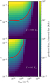 |
Fig. 9. Ratio of the predicted flux from our BH population and the observed limits in the soft band (0.3–2 keV; shown by the color bar). The y-axis shows the possible values for |
3.2.4. Black hole activity and metallicity
To assess the joint constraints on BH activity (parameterized through k) and the metallicity of the shielding column, we again adopted our reference model with a generic column of Nave = 1020 cm−2. We started the analysis with an unobscured region, that is, as shown in Fig. 8, a region with Nave = 1020 cm−2, where the resulting X-ray flux exceeds the upper limits for the range of metallicities considered here, except for values of k ≲ 10−3.
For the soft band, the region restricted to k > 6 × 10⁻³ and Z ≲ 0.2 Z⊙ overpredicts the upper limit of the flux by a factor of ∼100. A low average column density of ∼1020 cm−2 would thus then also require k ≲ 6 × 10⁻³ for metallicities ranging from 1 − 0.01 Z⊙.
On the other hand, for high-redshift BHs, we expect higher values of the duty cycle and the Eddington ratio, even when the precise value of k is unconstrained. The situation improves quite relevantly with a higher column density of Nave = 1021 cm−2, for which even values of k ∼ 0.3 become compatible with the constraints when the metallicity is high. Even at lower metallicities, this effect can likely be mitigated by higher gas columns increasing the amount of shielding. The overall constraints for this case are summarized in Fig. 10 as a function of metallicity and as a function of k.
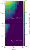 |
Fig. 10. Ratio of the predicted flux from our BH population and the observed limits in the soft band (0.3–2 keV). The solid red line denotes the curve where the ratio of the predicted flux and the observed one is equal to one. The x-axis shows the metallicities from solar to Z = 0.01 Z⊙. The y-axis is the k parameter. We adopted an average column density Nave = 1020 cm−2 (top panel) and Nave = 1021 cm−2 (bottom panel). |
3.3. Comparison with IR-inferred black hole masses
In this section, we compare our predictions with BH masses inferred from the luminosities in the F444W band. We converted the apparent magnitudes into flux densities (fF444W) and subsequently into bolometric luminosities (Lbol) using a BC, such that Lbol = BC ⋅ 4πDL2νfF444W. Assuming the source radiates at a specific Eddington fraction, ϵEdd, we estimated the BH mass as
 (11)
(11)
We adopted three different BCs from Greene et al. (2026): BC = 8 (standard), BC = 3.1 (minimum), and BC = 21.0 (maximum), reflecting the uncertainty in the SEDs of LRDs. Exploring this range allowed us to bracket the possible BH masses despite the lack of calibrated corrections for this population.
In Fig. 11 we compare these IR-inferred masses with our reference collision model (α = 1, β = 0.6; red histogram). The top panel assumes a moderate Eddington fraction of ϵEdd = 10−3. In this scenario, the peak of our model distribution (∼107 M⊙) is consistent with the bulk of the IR-inferred masses (green and orange lines). However, we explicitly note a discrepancy in the distribution widths: while the IR-derived masses span a broad range extending to > 108 M⊙, our model is strictly capped at ∼107 M⊙ by the validation limit of the collisional channel.
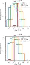 |
Fig. 11. Distribution of BH masses inferred with the luminosities obtained from the mF444W magnitude, compared to our reference model α = 1 and β = 0.6 (filled red histogram). The top panel assumes an Eddington fraction ϵEdd = 10−3. The bottom panel assumes ϵEdd = 10−4. The colored lines show the mass distributions for the standard (BC = 8.0, green), minimum (BC = 3.1, blue), and maximum BC (BC = 21.0, orange). |
The bottom panel (ϵEdd = 10−4) shows consistency with the minimum BC (blue line). We further explore the high-accretion regime (ϵEdd = 0.3) in Appendix D, finding that such high ratios would result in predicted BH masses that significantly exceed those estimated from IR observations. This reinforces our conclusion that the LRD population is best described by heavy seeds accreting at a moderate to low efficiency or with low duty cycles.
4. Summary and discussions
We provided estimates for the possible masses of SMBHs formed in LRDs via collisions. For this purpose, we presented a toy-model assuming a power-law evolution of the stellar mass with time with a power-law index α, as well as a mass-radius relation where the radius scales as mass to the power β. We included a BH formation scenario based on runaway stellar collisions using stellar systems with collisional timescales shorter than their age, which was motivated by previous studies (Escala 2021; Escala et al. 2025; Vergara et al. 2023, 2024, 2025; Vergara et al. 2026). We found that the possibility of forming massive BHs is particularly sensitive to the parameter β ( ), which should be about 0.6 or higher for the collision-based channel to be highly efficient. In this case, it is capable to produce SMBHs considerably above the BH mass – bulge mass relation observed in the local Universe (e.g., Reines & Volonteri 2015), while consistent with high-redshift data such as Harikane et al. (2023), Maiolino et al. (2024). Even for values of β ∼ 0.6, which are more typical for spiral galaxies in the local Universe (Shen et al. 2003), high efficiencies of forming massive objects can still be obtained, in particular, when the value of α is above 1, implying that the SFR increases as a function of time. The range of α and β values was determined from purely theoretical considerations requiring collisions to be efficient while keeping β within a realistic range, and from considering the typical observed SFRs in LRDs. In addition, we verified that they were also compatible with the X-ray constraints in the regime of low column densities (for a strongly obscured system as proposed by Maiolino et al. (2025), no constraints can be obtained). We generally emphasize that the derived constraints from the X-ray background are only valid in the regime where obscuration is not significant, as otherwise, clearly, no relevant constraints could be obtained.
High-z galaxies are observed to have an increasing star formation history (Topping et al. 2022). Cosmological simulations using high-resolution radiation-hydrodynamic suggest that the SFR grows exponentially (Pallottini et al. 2017; Pallottini & Ferrara 2023). We note that even when the SFR is constant (α = 1) or decreases with time (α < 1), massive BHs are still likely to form, but at a reduced mass, but their further growth would still be possible via accretion, possibly even at super-Eddington rates (e.g., Inayoshi et al. 2016; Takeo et al. 2019; Regan et al. 2019). There are observational constraints that seem to unfavorably affect super-Eddington accretion in the current stage of their evolution, although it may be too early to conclude about possible previous phases, where the main uncertainty is how long super-Eddington accretion lasts (Volonteri et al. 2021).
The intrinsic X-ray emission model included an external attenuation from column densities (Nave) with different metallicities (Z). We introduced a parameter for the overall X-ray activity  that depends on the fraction of sources with a massive BH
  , the duty cycle Uduty, the Eddington ratio ϵEdd, and the fraction of the bolometric luminosity emitted in X-rays ϵX. We used this framework to derive the expected soft and hard X-ray emission from the sample of S+25. We note that, although the radii of the LRDs in their sample have not been released to the public, we assumed that they follow the same distribution as the sample of A+24. We then used a Monte-Carlo approach to assign initial radii to sources. This allowed us to compare the expected emission to the upper limits that S+25 derived via stacking techniques from the CDF-S, corresponding to a total exposure time of 400 Ms. High X-ray activity levels, corresponding to high values of k, are feasible but require higher column densities and/or higher levels of metal enrichment in these columns, as the heavy elements significantly increase the cross section for X-ray absorption.
Our collision-based BH formation scenario provides a natural explanation for the detection of overly massive BHs and reconciles their presence with the reported weakness of X-ray signals without requiring high levels of obscuration. For our most extreme case, in which all the BHs continuously accrete and emit 30% of their Eddington luminosity in X-rays, a column density of only Nave ∼ 3 × 1018 cm−2 at solar metallicity is required to be compatible with the observational constraints, while at lower metallicities (Z = 10−2 Z⊙), a column density of Nave ∼ 2 × 1021 cm−2 is enough to reduce the X-ray emission. However, as explored in Appendix C, the subsequent growth should then be well-regulated to be compatible with the X-ray constraints, at least for the typical population. A moderate sub-Eddington accretion rate (L/LEdd ≈ 0.1) (consistent with typical type 1 AGNs) provides a plausible explanation for the existence of accretion. Nonetheless, we also point out that JWST has even found some more peculiar sources with BH-to-bulge mass ratios of about 40% (Juodžbalis et al. 2024). In these cases, the combination of high seed masses with very efficient accretion might be a promising way to explain the extreme outcomes in the more extreme sources. More extreme scenarios in which β takes on higher values (β ≳ 1.2), resulting in significantly earlier seed formation times and consequently altering the requirements for the subsequent accretion history and duty cycles, are discussed in detail in Appendix C.
Latif et al. (2025) recently explored the expected radio signatures of LRDs. Their analysis indicates that the radio flux from the AGN component generally dominates the stellar component, often by factors of 10 − 100, particularly for lower SFRs (< 10 M⊙ yr−1). However, at higher SFRs (≥10 − 30 M⊙ yr−1), which our models and cited observations suggest are plausible for LRDs (Fig. 5), the radio emission linked to star formation can become comparable to or can even exceed that of a radio-quiet AGN. While deeper observations hold promise for detecting these radio-quiet signals, the potential contamination from intense star formation activity underscores the challenge of using radio emission alone to unambiguously confirm the AGN nature of LRDs when SFRs are high. This highlights the complementary importance of X-ray constraints, such as those presented in this work, which can help us to disentangle the contributions even in highly star-forming dusty environments.
A crucial next step is to directly constrain the gas content of LRDs. The presence of a substantial gas reservoir would deepen the central gravitational potential and enhance the rate of dynamical interactions and stellar collisions, which might affect the assembly of compact stellar systems and the fueling of central BHs (e.g., Boekholt et al. 2018; Tagawa et al. 2020; Reinoso et al. 2020; Schleicher et al. 2022; Reinoso et al. 2023; Solar et al. 2025). Second, measurements of gas columns are necessary to distinguish between different physical interpretations of LRDs: scenarios such as heavily obscured active nuclei or compact starbursts depend sensitively on the assumed hydrogen column density, with obscured AGN models typically requiring NH ≳ 1023 cm−2 (e.g., Hickox & Alexander 2018), while star-forming or unobscured models are consistent with much lower values. Therefore, direct determinations of gas mass and column density are essential for understanding the internal dynamics of these systems and for ruling out competing formation pathways.
Acknowledgments
ML gratefully acknowledges support from ANID/DOCTORADO BECAS CHILE 72240058. DRGS gratefully acknowledges the support of the ANID BASAL project FB21003 and the Alexander von Humboldt – Foundation, Bonn, Germany. MCV acknowledges funding through ANID (Doctorado acuerdo bilateral DAAD/62210038) and DAAD (funding program number 57600326). MCV acknowledges the International Max Planck Research School for Astronomy and Cosmic Physics at the University of Heidelberg (IMPRS-HD). This material is based upon work supported by Tamkeen under the NYU Abu Dhabi Research Institute grant CASS.
References
- Akins, H. B., Casey, C. M., Allen, N., et al. 2023, ApJ, 956, 61 [NASA ADS] [CrossRef] [Google Scholar]
- Akins, H. B., Casey, C. M., Lambrides, E., et al. 2025, ApJ, 991, 37 [Google Scholar]
- Allen, N., Oesch, P. A., Toft, S., et al. 2025, A&A, 698, A30 [NASA ADS] [CrossRef] [EDP Sciences] [Google Scholar]
- Ananna, T. T., Bogdán, Á., Kovács, O. E., Natarajan, P., & Hickox, R. C. 2024, ApJ, 969, L18 [NASA ADS] [CrossRef] [Google Scholar]
- Anderson, M. E., Gaspari, M., White, S. D. M., Wang, W., & Dai, X. 2015, MNRAS, 449, 3806 [NASA ADS] [CrossRef] [Google Scholar]
- Baggen, J. F. W., van Dokkum, P., Labbé, I., et al. 2023, ApJ, 955, L12 [NASA ADS] [CrossRef] [Google Scholar]
- Binney, J., Tremaine, S., & Freeman, K. 2009, Phys. Today, 62, 56 [NASA ADS] [CrossRef] [Google Scholar]
- Boekholt, T. C. N., Schleicher, D. R. G., Fellhauer, M., et al. 2018, MNRAS, 476, 366 [Google Scholar]
- Casey, C. M., Scoville, N. Z., Sanders, D. B., et al. 2014, ApJ, 796, 95 [NASA ADS] [CrossRef] [Google Scholar]
- Curti, M., Maiolino, R., Curtis-Lake, E., et al. 2024, A&A, 684, A75 [NASA ADS] [CrossRef] [EDP Sciences] [Google Scholar]
- Duncan, K., Conselice, C. J., Mortlock, A., et al. 2014, MNRAS, 444, 2960 [Google Scholar]
- Duras, F., Bongiorno, A., Ricci, F., et al. 2020, A&A, 636, A73 [NASA ADS] [CrossRef] [EDP Sciences] [Google Scholar]
- Eisenstein, D. J., Johnson, B. D., Robertson, B., et al. 2025, ApJS, 281, 50 [Google Scholar]
- Eisenstein, D. J., Willott, C., Alberts, S., et al. 2026, ApJS, 283, 6 [Google Scholar]
- Escala, A. 2021, ApJ, 908, 57 [NASA ADS] [CrossRef] [Google Scholar]
- Escala, A., Zimmermann, L., Valdebenito, S., et al. 2025, ApJ, 995, 44 [Google Scholar]
- Fujii, M. S., Wang, L., Tanikawa, A., Hirai, Y., & Saitoh, T. R. 2024, Science, 384, 1488 [NASA ADS] [CrossRef] [Google Scholar]
- Furtak, L. J., Zitrin, A., Plat, A., et al. 2023, ApJ, 952, 142 [NASA ADS] [CrossRef] [Google Scholar]
- Georgiev, I. Y., Böker, T., Leigh, N., Lützgendorf, N., & Neumayer, N. 2016, MNRAS, 457, 2122 [Google Scholar]
- Glikman, E., Rusu, C. E., Chen, G. C. F., et al. 2023, ApJ, 943, 25 [NASA ADS] [CrossRef] [Google Scholar]
- González, V., Labbé, I., Bouwens, R. J., et al. 2011, ApJ, 735, L34 [Google Scholar]
- Greene, J. E., Labbe, I., Goulding, A. D., et al. 2024, ApJ, 964, 39 [CrossRef] [Google Scholar]
- Greene, J. E., Setton, D. J., Furtak, L. J., et al. 2026, ApJ, 996, 129 [Google Scholar]
- Guia, C. A., Pacucci, F., & Kocevski, D. D. 2024, Res. Notes Am. Astron. Soc., 8, 207 [Google Scholar]
- Gültekin, K., Richstone, D. O., Gebhardt, K., et al. 2009, ApJ, 698, 198 [Google Scholar]
- Harikane, Y., Zhang, Y., Nakajima, K., et al. 2023, ApJ, 959, 39 [NASA ADS] [CrossRef] [Google Scholar]
- Hickox, R. C., & Alexander, D. M. 2018, ARA&A, 56, 625 [Google Scholar]
- Ho, L. C. 2008, ARA&A, 46, 475 [Google Scholar]
- Inayoshi, K., Haiman, Z., & Ostriker, J. P. 2016, MNRAS, 459, 3738 [NASA ADS] [CrossRef] [Google Scholar]
- Juodžbalis, I., Maiolino, R., Baker, W. M., et al. 2024, Nature, 636, 594 [CrossRef] [Google Scholar]
- Killi, M., Watson, D., Brammer, G., et al. 2024, A&A, 691, A52 [NASA ADS] [CrossRef] [EDP Sciences] [Google Scholar]
- Kocevski, D. D., Onoue, M., Inayoshi, K., et al. 2023, ApJ, 954, L4 [NASA ADS] [CrossRef] [Google Scholar]
- Kocevski, D. D., Finkelstein, S. L., Barro, G., et al. 2025, ApJ, 986, 126 [Google Scholar]
- Labbe, I., Greene, J. E., Matthee, J., et al. 2024, ArXiv e-prints [arXiv:2412.04557] [Google Scholar]
- Labbe, I., Greene, J. E., Bezanson, R., et al. 2025, ApJ, 978, 92 [NASA ADS] [CrossRef] [Google Scholar]
- Lange, R., Driver, S. P., Robotham, A. S. G., et al. 2015, MNRAS, 447, 2603 [CrossRef] [Google Scholar]
- Latif, M. A., Aftab, A., Whalen, D. J., & Mezcua, M. 2025, A&A, 694, L14 [NASA ADS] [CrossRef] [EDP Sciences] [Google Scholar]
- Lee, K.-S., Ferguson, H. C., Wiklind, T., et al. 2012, ApJ, 752, 66 [NASA ADS] [CrossRef] [Google Scholar]
- Liempi, M., Schleicher, D. R. G., Benson, A., Escala, A., & Vergara, M. C. 2025, A&A, 694, A42 [NASA ADS] [CrossRef] [EDP Sciences] [Google Scholar]
- Liu, T., Tozzi, P., Wang, J.-X., et al. 2017, ApJS, 232, 8 [NASA ADS] [CrossRef] [Google Scholar]
- Madau, P., & Haardt, F. 2024, ApJ, 976, L24 [Google Scholar]
- Maiolino, R., Scholtz, J., Curtis-Lake, E., et al. 2024, A&A, 691, A145 [NASA ADS] [CrossRef] [EDP Sciences] [Google Scholar]
- Maiolino, R., Risaliti, G., Signorini, M., et al. 2025, MNRAS, 538, 1921 [Google Scholar]
- Matthee, J., Naidu, R. P., Brammer, G., et al. 2024, ApJ, 963, 129 [NASA ADS] [CrossRef] [Google Scholar]
- Meyer, R. A., Oesch, P. A., Giovinazzo, E., et al. 2024, MNRAS, 535, 1067 [CrossRef] [Google Scholar]
- Nagao, T., Maiolino, R., & Marconi, A. 2006, A&A, 459, 85 [NASA ADS] [CrossRef] [EDP Sciences] [Google Scholar]
- Neumayer, N., Seth, A., & Böker, T. 2020, A&ARv, 28, 4 [Google Scholar]
- Oke, J. B. 1974, ApJS, 27, 21 [Google Scholar]
- Ormerod, K., Conselice, C. J., Adams, N. J., et al. 2024, MNRAS, 527, 6110 [Google Scholar]
- Pacucci, F., Hernquist, L., & Fujii, M. 2025, ApJ, 994, 40 [Google Scholar]
- Pallottini, A., & Ferrara, A. 2023, A&A, 677, L4 [NASA ADS] [CrossRef] [EDP Sciences] [Google Scholar]
- Pallottini, A., Ferrara, A., Bovino, S., et al. 2017, MNRAS, 471, 4128 [NASA ADS] [CrossRef] [Google Scholar]
- Pérez-González, P. G., Barro, G., Rieke, G. H., et al. 2024, ApJ, 968, 4 [CrossRef] [Google Scholar]
- Piconcelli, E., Jimenez-Bailón, E., Guainazzi, M., et al. 2005, A&A, 432, 15 [NASA ADS] [CrossRef] [EDP Sciences] [Google Scholar]
- Planck Collaboration VI. 2020, A&A, 641, A6 [NASA ADS] [CrossRef] [EDP Sciences] [Google Scholar]
- Regan, J. A., Downes, T. P., Volonteri, M., et al. 2019, MNRAS, 486, 3892 [CrossRef] [Google Scholar]
- Reines, A. E., & Volonteri, M. 2015, ApJ, 813, 82 [NASA ADS] [CrossRef] [Google Scholar]
- Reinoso, B., Schleicher, D. R. G., Fellhauer, M., Leigh, N. W. C., & Klessen, R. S. 2020, A&A, 639, A92 [NASA ADS] [CrossRef] [EDP Sciences] [Google Scholar]
- Reinoso, B., Klessen, R. S., Schleicher, D., Glover, S. C. O., & Solar, P. 2023, MNRAS, 521, 3553 [CrossRef] [Google Scholar]
- Ricci, C., Trakhtenbrot, B., Koss, M. J., et al. 2017, ApJS, 233, 17 [Google Scholar]
- Rinaldi, P., Bonaventura, N., Rieke, G. H., et al. 2025, ApJ, 992, 71 [Google Scholar]
- Sacchi, A., & Bogdán, Á. 2025, ApJ, 989, L30 [Google Scholar]
- Sanders, R. L., Shapley, A. E., Topping, M. W., Reddy, N. A., & Brammer, G. B. 2024, ApJ, 962, 24 [NASA ADS] [CrossRef] [Google Scholar]
- Schleicher, D. R. G., Reinoso, B., Latif, M., et al. 2022, MNRAS, 512, 6192 [NASA ADS] [CrossRef] [Google Scholar]
- Shakura, N. I., & Sunyaev, R. A. 1973, A&A, 24, 337 [NASA ADS] [Google Scholar]
- Shapiro, S. L. 2005, ApJ, 620, 59 [NASA ADS] [CrossRef] [Google Scholar]
- Shen, S., Mo, H. J., White, S. D. M., et al. 2003, MNRAS, 343, 978 [NASA ADS] [CrossRef] [Google Scholar]
- Shibuya, T., Ouchi, M., & Harikane, Y. 2015, ApJS, 219, 15 [Google Scholar]
- Solar, P. A., Reinoso, B., Schleicher, D. R. G., Klessen, R. S., & Banerjee, R. 2025, A&A, 699, A64 [NASA ADS] [CrossRef] [EDP Sciences] [Google Scholar]
- Soltan, A. 1982, MNRAS, 200, 115 [Google Scholar]
- Song, M., Finkelstein, S. L., Ashby, M. L. N., et al. 2016, ApJ, 825, 5 [NASA ADS] [CrossRef] [Google Scholar]
- Stefanon, M., Bouwens, R. J., Labbé, I., et al. 2021, ApJ, 922, 29 [NASA ADS] [CrossRef] [Google Scholar]
- Tagawa, H., Haiman, Z., & Kocsis, B. 2020, ApJ, 892, 36 [Google Scholar]
- Takeo, E., Inayoshi, K., Ohsuga, K., Takahashi, H. R., & Mineshige, S. 2019, MNRAS, 488, 2689 [NASA ADS] [CrossRef] [Google Scholar]
- Topping, M. W., Stark, D. P., Endsley, R., et al. 2022, MNRAS, 516, 975 [NASA ADS] [CrossRef] [Google Scholar]
- Trump, J. R., Impey, C. D., Kelly, B. C., et al. 2009, ApJ, 700, 49 [Google Scholar]
- Vergara, M. C., Escala, A., Schleicher, D. R. G., & Reinoso, B. 2023, MNRAS, 522, 4224 [NASA ADS] [CrossRef] [Google Scholar]
- Vergara, M. C., Schleicher, D. R. G., Escala, A., et al. 2024, A&A, 689, A34 [NASA ADS] [CrossRef] [EDP Sciences] [Google Scholar]
- Vergara, M. C., Askar, A., Kamlah, A. W. H., et al. 2025, A&A, 704, A321 [NASA ADS] [CrossRef] [EDP Sciences] [Google Scholar]
- Vergara, M. C., Askar, A., Flammini Dotti, F., et al. 2026, A&A, 707, A71 [NASA ADS] [CrossRef] [EDP Sciences] [Google Scholar]
- Verner, D. A., Ferland, G. J., Korista, K. T., & Yakovlev, D. G. 1996, ApJ, 465, 487 [Google Scholar]
- Volonteri, M., Habouzit, M., & Colpi, M. 2021, Nat. Rev. Phys., 3, 732 [NASA ADS] [CrossRef] [Google Scholar]
- Wang, B., Leja, J., de Graaff, A., et al. 2024, ApJ, 969, L13 [NASA ADS] [CrossRef] [Google Scholar]
- Williams, C. C., Alberts, S., Ji, Z., et al. 2024, ApJ, 968, 34 [NASA ADS] [CrossRef] [Google Scholar]
- Wilms, J., Allen, A., & McCray, R. 2000, ApJ, 542, 914 [Google Scholar]
- Yang, G., Brandt, W. N., Luo, B., et al. 2016, ApJ, 831, 145 [NASA ADS] [CrossRef] [Google Scholar]
- Yang, G., Boquien, M., Buat, V., et al. 2020, MNRAS, 491, 740 [Google Scholar]
- Yue, M., Eilers, A.-C., Ananna, T. T., et al. 2024, ApJ, 974, L26 [CrossRef] [Google Scholar]
- Zappacosta, L., Piconcelli, E., Fiore, F., et al. 2023, A&A, 678, A201 [NASA ADS] [CrossRef] [EDP Sciences] [Google Scholar]
- Zhang, Y., Ding, X., Yang, L., et al. 2025, ArXiv e-prints [arXiv:2510.25830] [Google Scholar]
Note that the normalization of the correlation is individual for each source in order to match the final radius sampled from the distribution.
Appendix A: Markov chain Monte Carlo (MCMC) fitting
In Fig. A.3 we show the results of the best fit of the correlation Mgal − Rgal for the data sample of A+24. We assume a linear model in log space with intrinsic scatter log10σ,
 (A.1)
(A.1)
where A is the slope and B is the intercept parameter. In summary, our statistical model is described by θ = (A, B, log10σ).
The posterior distribution P(θ|D) is sampled using Bayes’ theorem, i.e.,
 (A.2)
(A.2)
with ℒ the likelihood function. We assume a Gaussian likelihood where the observed log10Mi for each galaxy is normally distributed (see Fig. A.1 for the mass distribution) around the model prediction (including the intrinsic scatter) as
![Mathematical equation: $$ \begin{aligned} \ln {\mathcal{L} (D|\theta )}=-0.5\sum _{i}\left[\frac{(\log _{10}M_i-(A\log _{10}R_i+B))^2}{\sigma ^2}-\ln (2\pi \sigma ^2) \right], \end{aligned} $$](/articles/aa/full_html/2026/04/aa58108-25/aa58108-25-eq46.gif) (A.3)
(A.3)
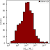 |
Fig. A.1. Mass distribution of the LRD galaxies in the A+24 sample. |
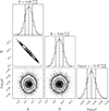 |
Fig. A.2. Marginalized one-dimensional (diagonal) and two-dimensional (off-diagonal) posterior probability distributions for the model parameters: slope (A), intercept (B), and log-scatter (log10σ). The diagonal histograms show the median (central line) and the 1σ intervals. A strong negative correlation is evident between the slope (A) and the intercept (B). |
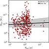 |
Fig. A.3. Data and model comparison of LRD galaxies in the A+24 sample. The dashed black line shows the mean value of the model introduced in Eq. A.1, while the shadow corresponds to the 1σ confidence interval. |
where we assume uniform priors over broad ranges to allow the data to dominate the inference. The values of the priors are listed in Table A.1.
Uniform priors π(θ) adopted for the MCMC analysis.
The posterior distribution was sampled using the emcee Python package. We used Nwalkers = 32 chains, where the chains were run for a total of 2000 steps. The burn-in phase of 250 steps was discarded to ensure the chains had fully converged to the stable posterior distribution. We verify convergence and adequate sampling by calculating the autocorrelation time τ for each parameter. The maximum τ observed was 16.63 steps. Since the chain length (2000 steps) significantly exceeded 50 × τ, we conclude that the samples were sufficiently independent and well mixed.
Our best-fit values are listed in Table A.2. The slope of the assumed correlation (A = 0.09 ± 0.10) is nearly flat. As the radius increases by a factor of 10, its mass, on average, increases only by a factor of ≈1.23. This suggests that galaxies are distributed across the log M − log R plane with a mass distribution that is primarily determined by factors other than size. We also emphasize that we consider the upper limits of the radius as almost all of the sources are not spatially resolved. More precise measurements of the radius and including more free parameters might change this analysis.
Best-fit parameters from MCMC analysis.
Appendix B: Sample comparisons
In this appendix we compare the properties of the A+24 sample, which we use to define the structural parameters of LRDs, and the subsample of S+25 used for the X-ray analysis in this work.
In Fig. B.1 we compare the stellar mass distributions of the two samples. The A+24 sample (red) is peaked at high masses (Mgal ∼ 1010 − 1011 M⊙), while the S+25 subsample (blue) exhibits an extended tail of low-mass objects reaching down to 106 M⊙. We argue that the inclusion of lower-mass galaxies in the S+25 sample does not introduce a bias in our modeling. This is due to the inherent nature of X-ray stacking, where the aggregate signal is flux-weighted. Since the X-ray luminosity scales with stellar mass (LX ∝ Mgal; e.g., Anderson et al. 2015), the stacked signal is dominated by the most massive galaxies in the sample. A single galaxy with a mass of 1010 M⊙ contributes a flux comparable to thousands of 106 M⊙ systems. Therefore, the structural parameters of the massive end of the population (represented by the A+24 sample) are the relevant priors for modeling the sources responsible for the potential X-ray emission.
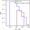 |
Fig. B.1. Comparison of the stellar mass distributions between the A+24 sample (red) and the S+25 subsample (blue). While the S+25 sample extends to lower masses, the X-ray stacking signal is dominated by the massive end of the population, justifying the use of structural parameters derived from the A+24 sample. |
In Fig. B.2 we show the redshift distributions. Both samples exhibit significant overlap in the z = 5 − 8 range, which dominates the stacking signal. However, the S+25 sample extends to lower (z ∼ 3) and higher (z ∼ 11) redshifts. We assume that the structural properties of LRDs remain comparable across this redshift window. For the high-redshift tail (z > 8), this is a conservative assumption. Galaxies at higher redshifts are theoretically and observationally expected to be more compact at fixed stellar mass (e.g., Shibuya et al. 2015; Allen et al. 2025). By applying the radius distribution from the slightly lower-redshift sample of A+24, we likely overestimate the physical sizes of these highest-redshift sources. In our collision-based model, larger radii imply lower stellar densities and, consequently, lower BH formation efficiencies. Thus, our approach likely underestimates the BH mass density at the high-redshift end, further strengthening our conclusions that collisional formation is a viable channel.
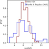 |
Fig. B.2. Comparison of the redshift distributions. The samples overlap significantly in the z = 5 − 8 range. For the high-redshift tail (z > 8) in the S+25 sample, our use of radii from the lower-redshift A+24 sample yields conservative estimates for stellar density and collisional efficiency. |
Appendix C: Effect of accretion in final black hole masses
In Fig. C.1 we map the average BH formation time (tform) as a fraction of the galaxy age (tage) across our parameter space of α and β. First, we note that in models with β ∼ 0.6, as in typical spiral galaxies in the local Universe, the seed BH tends to form rather late. In this case, not much time is available for subsequent growth. In this case, the accretion rate cannot be strongly constrained from the comparison with the observed BH masses, as the time window for accretion is relatively short. We nonetheless also report here about models where the seed BH forms at earlier stages, requiring more extreme assumptions about the β parameter. The colorbar, ⟨tform/tage⟩, reveals a strong trend in which models with high β (≳1.2) and low-to-intermediate α (∼0.5 − 1.0) produce BH seeds extremely early. In these extreme scenarios (dark purple region), seeds form, on average, when the galaxy is only about 10% of its current age (tform ≈ 0.1 tage). We investigate the implications of this early formation in Fig. C.2. We select a representative model from this extreme, early-forming regime: α = 0.7 and β = 1.4, and we calculate the final BH mass after a period of accretion.
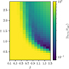 |
Fig. C.1. Average ratio between the BH formation time (tform) and the total age of the galaxy (tage) for each (α, β) model (see the colorbar). The y-axis shows the star formation parameter α, and the x-axis shows the mass-radius relation exponent β. Dark purple regions indicate very early seed formation (tform ≈ 0.1 tage), while yellow regions indicate very late formation (tform ≈ tage). |
We estimate the final mass Mf at a time t using the expression from Shapiro (2005), which describes exponential growth:
 (C.1)
(C.1)
where ti is the formation time of the BH seed (equivalent to tform from Fig. 1), Mi(ti) is the initial seed mass, and t is the final time (corresponding to the age of the galaxy, tage). The parameter ϵL = L/LEdd is the accretion luminosity as a fraction of the Eddington luminosity. The radiative efficiency, ϵM, is the fraction of accreted rest-mass energy converted to light (typically ∼0.1). The characteristic accretion timescale is τ = Mc2/LEdd, where M is the BH mass and c is the speed of light. Using this formalism, we analyze the results in Fig. C.2. Here, we select a representative model from the extreme, early-forming regime identified in Fig. C.2, specifically, the α = 0.7 and β = 1.4 model. We explore the impact of BH radiative efficiency (ϵM) and Eddington ratio (ϵL) on the final BH mass (MBH). The two panels contrast a low-efficiency model, observed in Quasars (e.g., Soltan 1982) with a typical value ϵM ∼ 0.1 (top panel) with a high-efficiency model ϵM = 0.42 (bottom panel) which is the upper limit for a thin accretion disk (Shakura & Sunyaev 1973), both applied to the same initial seed population (blue points). For the low radiative efficiency (ϵM = 0.1), 90% of the accreted mass is retained by the BH, leading to rapid and efficient mass growth. As a result, Eddington-limited (ϵL = 1, purple) and moderate sub-Eddington (ϵL = 0.1, brown) accretion rates produce final BH masses that are unphysically large. The ϵL = 1 case, in particular, results in growth factors of log(Mf/Mi)∼6 − 12, placing the final masses many orders of magnitude above the maximum ratio observed MBH/Mgal = 0.1 (dashed line). Even the ϵL = 0.1 rate produces growth factors of log(Mf/Mi)∼1 − 5, systematically overshooting the relation. Only a very low accretion rate (ϵL = 0.01, green) avoids this, but it produces negligible growth. Conversely, the bottom panel assumes a high radiative efficiency of ϵM = 0.42, the theoretical maximum corresponding to a maximally spinning Kerr BH. In this scenario, only 58% of the accreted mass is retained, leading to a much more gradual and self-regulated growth. Under this assumption, the model requires a sub-Eddington accretion scenario. We find that a moderate sub-Eddington rate of ϵL = 0.1 (brown points) is a physically plausible scenario. It produces a typical growth factor of ∼10. Furthermore, a low sub-Eddington rate (ϵL = 0.01, green) is also entirely viable, representing a quiescent population of BHs that have undergone minimal growth since their formation. By comparing these two physically motivated scenarios, we conclude that sub-Eddington accretion is not only a plausible mechanism but is in fact required to reconcile the initial seed masses with the present-day BH population. A model combining high radiative efficiencies (consistent with spinning BHs) and moderate sub-Eddington accretion rates (ϵL ≈ 0.1) provides an excellent framework for explaining the co-evolution of BHs and their host galaxies.
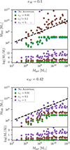 |
Fig. C.2. Top panel: BH mass versus host galaxy mass for a fiducial model with α = 0.7 and β = 1.4 assuming ϵM = 0.1. Blue dots show the initial seed masses (No Accretion). Green, brown and purple dots show the final mass after accretion with efficiencies ϵL = 0.01, ϵL = 0.1 and ϵL = 1, respectively. The dashed line shows the MBH/Mgal = 0.1 for reference. We also show the logarithmic ratio of the final (after accretion) mass to the initial mass for the models, quantifying the total BH growth. Bottom panel: Same as the top panel but here we set ϵM = 0.42 assuming that the BH is efficiently radiating. |
We emphasize that the conclusion above – that moderate sub-Eddington accretion is sufficient – relies on the adoption of a collision-favorable evolutionary track (α = 0.7, β = 1.4). In this regime, the BH seed forms with a significant fraction of the final mass. In contrast, for “standard” galaxy evolution scenarios (e.g., β ≈ 0.6, typical of local spirals), the collisional seeds are significantly smaller (Mseed ≪ Mfinal). Consequently, these scenarios require substantial mass growth via gas accretion to match the observed LRD BH masses. This implies a need for higher time-averaged accretion rates (higher k) or duty cycles approaching unity. As shown in our main analysis (Fig. 11), these accretion-dominated scenarios would result in X-ray fluxes that exceed the stacking upper limits unless extreme obscuration is invoked. Thus, the X-ray non-detections indirectly favor the ’heavy seed’ evolutionary paths where the duty cycle can remain low.
Appendix D: High accretion in IR-derived black hole masses
In Fig. D.1 we show the comparison between the distribution of BH masses derived from the mF444W magnitude assuming a high Eddington ratio ϵEdd = 0.3. In this case, our collision-based scenario would tend to over predict the BH masses estimated from the IR observations. For a high BC (BC = 21, orange distribution), the maximum BH masses estimated are closer to the ones predicted by our collisional model adopting α = 1.0 and β = 0.6.
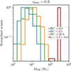 |
Fig. D.1. Distribution of BH masses inferred with the luminosities obtained from the mF444W magnitude, compared to our reference model α = 1 and β = 0.6 (filled red histogram). The top panel assumes an Eddington fraction ϵEdd = 10−3. The bottom panel assumes ϵEdd = 10−4. The colored lines show the mass distributions for the standard BC (BC = 8.0, green), the minimum (BC = 3.1, blue), and the maximum (BC = 21.0, orange). |
All Tables
All Figures
|
Fig. 1. Galaxy stellar masses obtained for the subsample of S+25 using the previous observed scaling correlation between MUV and Mgal (Eq. 1) compared to the stellar masses of the galaxies in the sample of A+24, both shown as a function of redshift. |
| In the text | |
|
Fig. 2. Probability density distribution of effective radii (Rgal) for the galaxy sample from A+24. The shaded red histogram shows the observed data binned in logarithmic intervals. The solid curves represent the best-fit Gaussian mixture models, assuming a single component (purple) and two components (cyan). We show the reduced chi-squared (χν2) for each model. |
| In the text | |
|
Fig. 3. Mass-radius diagram for stellar systems to illustrate relevant timescales and the position of different sources in different parts of the parameter space. The red dots show LRDs from A+24, gray dots show NSCs in the local Universe (Georgiev et al. 2016; Neumayer et al. 2020), blue dots show well-resolved BHs, and orange dots show spatially unresolved BHs (Gültekin et al. 2009; Escala 2021). The solid black line represents the collisional timescale tcoll = 13.7 Gyr, and the dashed black line shows the relaxation time for trelax = 13.7 Gyr. We include (in green) a fiducial galaxy with mass 1010 M⊙ and radius 20 pc to show its trajectory in the mass-radius plane for β = 1 and 0.5, as defined in Eq. (3). The time evolution of the green line is from left to right. |
| In the text | |
|
Fig. 4. Fraction of galaxies in which BH formation is driven by the condition t = tcoll as a function of the power-law exponents α and β . The x-axis represents the exponent in the mass-radius relation |
| In the text | |
|
Fig. 5. Distribution of the SFR of our galaxy sample as function of α. We show the distribution for α = 0.3 (blue), 1.0 (green), and 2.9 (orange). The cyan area shows the SFR range for the J0647_1045 galaxy at z ∼ 4.53 (Killi et al. 2024), the violet area shows the range of three LRDs at z ∼ 7 − 8 (Wang et al. 2024), and in gray, we show an extreme case of an LRD at z ∼ 4.47 with a high SFR (Labbe et al. 2024). |
| In the text | |
|
Fig. 6. MBH − Mgal relation from this work compared with observational results. All masses are given in solar masses (M⊙). The filled red area represents the parameter space spanned by the BH and host galaxy masses from this work for different combinations of α and β. In yellow we show the BH (and host galaxy) mass for α = 1.0 and β = 0.6 with a maximum mass seed of 107 M⊙. On the other hand, in green we show the masses without limiting the mass of the seed. The dashed black line and gray shaded area show the empirical MBH − Mgal relation for local (z = 0) galaxies (Reines & Volonteri 2015). We include data points from high-redshift (z = 4–7) observational studies from Harikane et al. (2023, blue open diamonds), data points from Maiolino et al. (2024, purple open squares), and from Zhang et al. (2025, cyan square). The dotted black lines indicate constant BH-to-galaxy mass ratios, labeled MBH/Mgal = 0.1 and 0.001. |
| In the text | |
|
Fig. 7. Panel (a): Soft X-ray band (0.3 − 2 keV). Panel (b): Hard X-ray band (2 − 7 keV). The color bar shows the ratio of the predicted and observed flux for the soft and hard bands. The allowed parameter space for α and β is the region where the ratio of the predicted flux to the observed flux is lower than 1, which satisfies the soft X-ray and hard X-ray observational constraints, respectively. The red line represents ratio of the predicted and observed flux equal to one. |
| In the text | |
|
Fig. 8. Ratio of the predicted flux from our BH population and the observed limits in the soft band (0.3–2 keV; shown by the color bar). The solid red line denotes the curve where the ratio of the predicted and observed flux is equal to one. The y-axis shows the metallicities from solar to Z = 0.01 Z⊙. The x-axis is the average column density Nave in units of cm−2. We adopted k = 0.3 as an example of an extreme case of high activity (top panel) and a more conservative value k = 2 × 10⁻³ (bottom panel). |
| In the text | |
|
Fig. 9. Ratio of the predicted flux from our BH population and the observed limits in the soft band (0.3–2 keV; shown by the color bar). The y-axis shows the possible values for |
| In the text | |
|
Fig. 10. Ratio of the predicted flux from our BH population and the observed limits in the soft band (0.3–2 keV). The solid red line denotes the curve where the ratio of the predicted flux and the observed one is equal to one. The x-axis shows the metallicities from solar to Z = 0.01 Z⊙. The y-axis is the k parameter. We adopted an average column density Nave = 1020 cm−2 (top panel) and Nave = 1021 cm−2 (bottom panel). |
| In the text | |
|
Fig. 11. Distribution of BH masses inferred with the luminosities obtained from the mF444W magnitude, compared to our reference model α = 1 and β = 0.6 (filled red histogram). The top panel assumes an Eddington fraction ϵEdd = 10−3. The bottom panel assumes ϵEdd = 10−4. The colored lines show the mass distributions for the standard (BC = 8.0, green), minimum (BC = 3.1, blue), and maximum BC (BC = 21.0, orange). |
| In the text | |
|
Fig. A.1. Mass distribution of the LRD galaxies in the A+24 sample. |
| In the text | |
|
Fig. A.2. Marginalized one-dimensional (diagonal) and two-dimensional (off-diagonal) posterior probability distributions for the model parameters: slope (A), intercept (B), and log-scatter (log10σ). The diagonal histograms show the median (central line) and the 1σ intervals. A strong negative correlation is evident between the slope (A) and the intercept (B). |
| In the text | |
|
Fig. A.3. Data and model comparison of LRD galaxies in the A+24 sample. The dashed black line shows the mean value of the model introduced in Eq. A.1, while the shadow corresponds to the 1σ confidence interval. |
| In the text | |
|
Fig. B.1. Comparison of the stellar mass distributions between the A+24 sample (red) and the S+25 subsample (blue). While the S+25 sample extends to lower masses, the X-ray stacking signal is dominated by the massive end of the population, justifying the use of structural parameters derived from the A+24 sample. |
| In the text | |
|
Fig. B.2. Comparison of the redshift distributions. The samples overlap significantly in the z = 5 − 8 range. For the high-redshift tail (z > 8) in the S+25 sample, our use of radii from the lower-redshift A+24 sample yields conservative estimates for stellar density and collisional efficiency. |
| In the text | |
|
Fig. C.1. Average ratio between the BH formation time (tform) and the total age of the galaxy (tage) for each (α, β) model (see the colorbar). The y-axis shows the star formation parameter α, and the x-axis shows the mass-radius relation exponent β. Dark purple regions indicate very early seed formation (tform ≈ 0.1 tage), while yellow regions indicate very late formation (tform ≈ tage). |
| In the text | |
|
Fig. C.2. Top panel: BH mass versus host galaxy mass for a fiducial model with α = 0.7 and β = 1.4 assuming ϵM = 0.1. Blue dots show the initial seed masses (No Accretion). Green, brown and purple dots show the final mass after accretion with efficiencies ϵL = 0.01, ϵL = 0.1 and ϵL = 1, respectively. The dashed line shows the MBH/Mgal = 0.1 for reference. We also show the logarithmic ratio of the final (after accretion) mass to the initial mass for the models, quantifying the total BH growth. Bottom panel: Same as the top panel but here we set ϵM = 0.42 assuming that the BH is efficiently radiating. |
| In the text | |
|
Fig. D.1. Distribution of BH masses inferred with the luminosities obtained from the mF444W magnitude, compared to our reference model α = 1 and β = 0.6 (filled red histogram). The top panel assumes an Eddington fraction ϵEdd = 10−3. The bottom panel assumes ϵEdd = 10−4. The colored lines show the mass distributions for the standard BC (BC = 8.0, green), the minimum (BC = 3.1, blue), and the maximum (BC = 21.0, orange). |
| In the text | |
Current usage metrics show cumulative count of Article Views (full-text article views including HTML views, PDF and ePub downloads, according to the available data) and Abstracts Views on Vision4Press platform.
Data correspond to usage on the plateform after 2015. The current usage metrics is available 48-96 hours after online publication and is updated daily on week days.
Initial download of the metrics may take a while.