| Issue |
A&A
Volume 700, August 2025
|
|
|---|---|---|
| Article Number | A138 | |
| Number of page(s) | 30 | |
| Section | Extragalactic astronomy | |
| DOI | https://doi.org/10.1051/0004-6361/202554648 | |
| Published online | 13 August 2025 | |
Luminous, rapidly declining supernovae as stripped transitional objects in low-metallicity environments: The case of SN 2022lxg
1
Department of Physics and Astronomy, University of Turku, FI-20014 Turku, Finland
2
The Oskar Klein Centre, Department of Astronomy, Stockholm University, AlbaNova, 10691 Stockholm, Sweden
3
Institut d’Estudis Espacials de Catalunya (IEEC), E-08034 Barcelona, Spain
4
Institute of Space Sciences (ICE, CSIC), Campus UAB, Carrer de Can Magrans, s/n, E-08193 Barcelona, Spain
5
Department of Physics, University of Warwick, Gibbet Hill Road, Coventry CV4 7AL, UK
6
Center for Interdisciplinary Exploration and Research in Astrophysics (CIERA), Northwestern University, 1800 Sherman Ave, Evanston, IL 60201, USA
7
Department of Astronomy, Kyoto University, Kitashirakawa-Oiwake-cho, Sakyo-ku, Kyoto 606-8502, Japan
8
Finnish Centre for Astronomy with ESO (FINCA), FI-20014 University of Turku, Finland
9
Yunnan Observatories, Chinese Academy of Sciences, Kunming 650216, PR China
10
International Centre of Supernovae, Yunnan Key Laboratory, Kunming 650216, PR China
11
Key Laboratory for the Structure and Evolution of Celestial Objects, Chinese Academy of Sciences, Kunming 650216, PR China
12
Caltech Optical Observatories, California Institute of Technology, Pasadena, CA 91125, USA
13
Division of Physics, Mathematics and Astronomy, California Institute of Technology, Pasadena, CA 91125, USA
14
Astrophysics Research Institute, Liverpool John Moores University, 146 Brownlow Hill, Liverpool L3 5RF, UK
15
IPAC, California Institute of Technology, 1200 E. California Blvd, Pasadena, CA 91125, USA
16
School of Sciences, European University Cyprus, Diogenes Street, Engomi, 1516 Nicosia, Cyprus
17
INAF – Osservatorio Astronomico di Brera, Via E. Bianchi 46, I23807 Merate, (LC), Italy
18
INAF – Osservatorio Astronomico di Padova, Vicolo dell’Osservatorio 5, I-35122 Padova, Italy
19
Cosmic Dawn Center (DAWN), Niels Bohr Institute, University of Copenhagen, 2200 Copenhagen, Denmark
20
Niels Bohr Institute, University of Copenhagen, Jagtvej 128, 2200 København N, Denmark
21
Department of Physics and Astronomy, Aarhus University, Ny Munkegade 120, DK-8000 Aarhus C, Denmark
22
INAF – Osservatorio Astronomico d’Abruzzo, Via Mentore Maggini snc, I-64100 Teramo, Italy
23
Anton Pannekoek Institute for Astronomy, University of Amsterdam, 1090 GE Amsterdam, The Netherlands
⋆ Corresponding author: This email address is being protected from spambots. You need JavaScript enabled to view it.
Received:
19
March
2025
Accepted:
12
June
2025
Abstract
We present an analysis of the optical and near-infrared properties of SN 2022lxg, a bright (Mg peak = −19.41 mag) and rapidly evolving supernova (SN). It was discovered within a day of explosion, and rose to peak brightness in ∼10 d. Two distinct phases of circumstellar interaction are evident in the data. The first is marked by a steep blue continuum (T > 15 000 K) with flash-ionisation features due to hydrogen and He II. The second, weaker phase is marked by a change in the colour evolution accompanied by changes in the shapes and velocities of the spectral line profiles. Narrow P-Cygni profiles (∼150 km s−1) of He I further indicate the presence of slow-moving, unshocked material and suggest partial stripping of the progenitor. The fast decline of the light-curve from the peak (3.48 ± 0.26 mag (50 d)−1 in g band) implies that the ejecta mass must be low. Spectroscopically, until +35 d there are similarities with some Type IIb SNe but then there is a transition to spectra that are more reminiscent of an interacting SN II. However, metal lines are largely absent in the spectra, even at epochs of ∼80 d. Its remote location (∼4.6 kpc projected offset) from the presumed host galaxy, a dwarf with MB ∼ −14.4 mag, is consistent with our metallicity estimate – close to the values of the Small Magellanic Cloud – obtained from scaling relations. Furthermore, several lines of evidence (including intrinsic polarisation of p ∼ (0.5 − 1.0)%) point to deviations from spherical symmetry. We suggest that a plausible way of uniting the observational clues is to consider a binary system that underwent case C mass transfer. This failed to remove the entire H envelope of the progenitor before it underwent core collapse. In this scenario, the progenitor itself would be more compact and perhaps straddle the boundary between blue and yellow supergiants, which ties in with the early spectroscopic similarity to Type IIb SNe.
Key words: circumstellar matter / stars: mass-loss / supernovae: general / supernovae: individual: SN 2022lxg
© The Authors 2025
 Open Access article, published by EDP Sciences, under the terms of the Creative Commons Attribution License (https://creativecommons.org/licenses/by/4.0), which permits unrestricted use, distribution, and reproduction in any medium, provided the original work is properly cited.
This article is published in open access under the Subscribe to Open model. This email address is being protected from spambots. You need JavaScript enabled to view it. to support open access publication.
1. Introduction
It is well accepted that the evolution of massive (≳8 M⊙) stars is primarily driven by mass loss, be it via line- or continuum-driven winds, Eta-Carina-type giant outbursts, other variabilities, or even due to a binary companion (e.g. Meynet et al. 1994; Langer 1998, 2012; Woosley et al. 2002). Thus, the immediate environment into which a massive star explodes is modified by these processes. Regardless of how the mass loss happens, the distribution and extent of this circumstellar material (CSM), as well as its composition, velocity, and amount can be indelibly imprinted onto observations of the supernova (SN).
A clear signature of interaction between SN ejecta and the surrounding medium is the presence of narrow (tens to hundreds of km s−1) emission lines (Schlegel 1990). At the earliest epochs after explosion, radiation from the shock breakout ionises this material, which results in prominent narrow emission features associated with species such as He II, C IV, and NIII/IV (often dubbed ‘flash features’). As the shock propagates through the CSM, a fraction of the kinetic energy of the ejecta is converted to energetic photons; these contribute to maintaining the high ionisation levels, which compensates for the relatively short recombination timescales of the ionised species. As the CSM gas is swept up by the fast-moving ejecta, the temperature drops and the narrow emission lines become weaker, ultimately giving way to a nearly featureless continuum, followed by the emergence of broad SN features (e.g. Chugai 2001; Fransson et al. 2005; Gal-Yam et al. 2014; Shivvers et al. 2015; Khazov et al. 2016; Yaron et al. 2017; Dessart et al. 2017; Bruch et al. 2021, 2023; Jacobson-Galán et al. 2024). The duration of this phase is strongly dependent on the spatial extent and density of the surrounding material, but typically lasts for approximately a week in most cases (Bruch et al. 2021). This implies that the material is spatially confined, and originates from presumably enhanced mass-loss shortly (months to a few years) prior to core collapse.
In the single star framework and roughly solar metallicities, we expect an inverse correlation between progenitor mass and the amount of hydrogen remaining in the envelope at the time of explosion. This translates into a sequence of SN subtypes with the Type II-plateau (IIP) progenitors having the thickest H envelopes, while the Type Ic progenitors, at the other extreme, have lost both H and He layers. Between these, we find the II-linear (IIL), IIb, and Ib subtypes that reflect a transition from a H-dominated envelope to a He-dominated one. Although the above framework is appealing and borne out by observations, we both expect and find a significant contribution from binary systems. Indeed, several studies have argued that a close binary companion is necessary to efficiently remove the H and He layers (e.g. Nomoto et al. 1993, 1995; Claeys et al. 2011; Yoon et al. 2017; Ercolino et al. 2024). Within either single or binary progenitor frameworks, we might also expect to find a continuum of observed properties (e.g. peak luminosity, duration). These will primarily depend on the specifics of the mass and mass-loss history, and the conditions in the core at the time of collapse, for each case.
Within this multi-dimensional parameter space, SNe that display extreme properties usually in terms of peak absolute brightness or decline rate from peak, often stand out (e.g. Barbary et al. 2009; Miller et al. 2009; Gezari et al. 2009). While several systematic studies of regular SNe II have been conducted, which have incorporated an increasing number of events over the years, most do not include objects with rest-frame light-curve peaks exceeding ∼ − 18.5 mag in the V band, that is, luminous SNe (LSNe II; e.g. Anderson et al. 2014a; Valenti et al. 2016). However, a growing number of such events have been identified. These luminous objects were already noted by Patat et al. (1994), who analysed a sample of 51 SNe II and highlighted a gap between regular SNe II and brighter events (−18.5 mag in the B band). More recently, Pessi et al. (2023a) (P23 hereafter) considered a sample of six SNe II with peak V band magnitudes brighter than −18.5, persistent blue colours, and fast decline rates. Spectroscopically, the Balmer lines showed broad, multi-component emission profiles over the time span of the observations (∼10 − 100 d for most of the sample), and metal lines were weak if at all present. Type II SNe that are brighter than −18.5 mag at peak in the optical region are unlikely to be missed by transient discovery surveys, and must therefore be rare. It is important to understand whether they arise from some unique combination of parameters, or whether they simply represent the tail of the Type II parameter distribution with a preferred viewing angle.
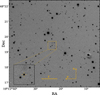 |
Fig. 1. r band image showing SN 2022lxg (α = 19h15m23.630s, δ = +48° 19′27.70″, J2000), taken with NOT+ALFOSC on 25 July 2022 (+54.2 d). The inset shows the region around the SN; no obvious host galaxy is apparent. |
On 4 June 2022, the All-Sky Automated Survey for Supernovae (ASAS-SN; Shappee et al. 2014) collaboration reported the discovery of a rising transient (ASASSN-22hp, IAU name: AT 2022lxg) in an uncatalogued host galaxy (Stanek 2022) to the Transient Name Server. Four days later, on 8 June 2022, the transient was classified as a SN II (SN 2022lxg) based on a blue and featureless spectrum (Ashall 2022). Given the excellent explosion epoch constraints, the rapid rise to a peak absolute brightness of −19.3 in the r band, and the presence of narrow emission lines in the spectrum at +2 d, we embarked on an observational campaign to monitor its evolution. We show the field of the SN in Fig. 1. As no redshift information was available for the presumed host galaxy, we measured the redshift of SN 2022lxg to be z = 0.0214 ± 0.0006, from the centroid of Hα and Hβ lines in the late time spectra (+65 and +80 d). Correcting the spectra with this value results in the flash-ionisation lines in the early spectra (Hα, Hβ and He IIλ4686) being at their respective rest wavelengths (Sect. 3.3).
Basic properties of SN 2022lxg.
In what follows, we present the follow-up and analysis of SN 2022lxg. We assume a Planck Collaboration ΛCDM cosmology with H0 = 67.4 km s−1 Mpc−1, Ωm = 0.315, and ΩΛ = 0.685 (Planck Collaboration VI 2020). The redshift, as inferred above, corresponds to a distance of 96.6 Mpc and distance modulus of μ = 34.925. All phases are given relative to the estimated explosion epoch (MJD = 59 731.37) in the transient rest-frame (Sect. 3.2.1). Magnitudes are in the AB system (Oke & Gunn 1983) unless noted otherwise, and the reported uncertainties correspond to 68% (1σ) and upper limits to 3σ.
2. Observations and data reduction
We acquired well-sampled imaging and spectroscopy, and three epochs of imaging polarimetry from a range of telescopes (Sect. 2). There is no evidence for host reddening in the spectra given the blue slope at early times and lack of absorption features due to the Na I D lines; hence we consider the host reddening to be negligible. Throughout this work, we assume a Cardelli et al. (1989) extinction law with RV = 3.1 and a foreground Galactic extinction of AV = 0.1815 mag (Schlafly & Finkbeiner 2011), to deredden our photometry and spectra.
2.1. Ground-based imaging
We obtained gri imaging with a roughly 2 − 3 d cadence via the Zwicky Transient Facility (ZTF; Graham et al. 2019; Bellm et al. 2019; Dekany et al. 2020), the Palomar Schmidt 48-inch (P48) Samuel Oschin and the Spectral Energy Distribution Machine Rainbow Camera on the Palomar 60-inch telescope (SEDM; Blagorodnova et al. 2018; Kim et al. 2022). These data were processed using the ZTF forced photometry service1 (Masci et al. 2019) and FPipe (Fremling et al. 2016), respectively. Further imaging obtained at the Liverpool Telescope (LT; Steele 2004) with the IO:O imager in the griz filters was reduced using custom pipelines, while light-curves using imaging from the Asteroid Terrestrial-impact Last Alert System (ATLAS; Tonry et al. 2018; Smith et al. 2020) survey in the o and c bands were generated using the ATLAS Forced Photometry2 service (Shingles et al. 2021). Two epochs of late-time (> 250 d) imaging were obtained with the Alhambra Faint Object Spectrograph and Camera (ALFOSC) mounted on the 2.56 m Nordic Optical Telescope (NOT) on La Palma, Spain. The complete, dereddened optical light-curves are shown in Fig. 2 and tabulated (non-dereddened) in Table A.1.
 |
Fig. 2. Light-curves of SN 2022lxg (corrected for MW extinction; E(B − V)MW = 0.059 mag). The explosion epoch is constrained to MJD 59 731.37. The short vertical black dashes denote the epochs of spectroscopy (see Table A.2). Non-detections are shown as small downward-facing arrows. The 56Co decay rate is shown as a dashed black line. Note the break in the x-axis to accommodate the latest epochs. The inset focuses on the phases around the peak light (for the gri bands). The g band seems to plateau for ∼ eight days at its peak (horizontal dashed line is a linear fit to guide the eye), while the r band shows a bump around the time of the start of the g-band plateau, but then continues to rise to its main peak. We show the Gaussian process interpolations used to infer the peak epochs in the gri bands (with 1σ uncertainties as shaded regions), which are marked with short vertical dashes (see also Table 1). |
2.2. Optical spectroscopy
We were able to collect 28 spectra of SN 2022lxg spanning ∼2 − 90 d. The earliest spectrum was obtained using the Low-Resolution Imaging Spectrometer (LRIS; Oke et al. 1995) on the Keck I 10-m telescope and reduced using lpipe (Perley et al. 2019). Spectra obtained using SEDM were reduced as described in Rigault et al. (2019); those collected with the Double Beam Spectrograph (DBSP) on the Palomar 200-in telescope were reduced using custom pipeline (Mandigo-Stoba et al. 2022) based on PypeIt (Prochaska et al. 2020). An LT spectrum was obtained with SPRAT instrument (Piascik et al. 2014) and reduced using the automated LT pipeline (Barnsley et al. 2012). All other spectra were obtained using the ALFOSC instrument on the NOT as part of the ZTF and NUTS2 (NOT Un-biased Transient Survey 2) collaborations. Reductions were performed using Foscgui3. The spectra were scaled with the available gri photometry. The spectral series, scaled with the photometry and dereddened for Milky Way (MW) extinction, are presented in Fig. 3 and a spectroscopic log is provided in Table A.2.
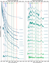 |
Fig. 3. Spectral series of SN 2022lxg (scaled with the photometry and corrected for MW extinction). Emission lines are marked with vertical dashed lines; throughout the evolution of SN 2022lxg, we detect Balmer lines, He Iλ5876, a broad blend of Fe II (∼5300 Å), and the Ca II NIR triplet. Other marked species are to guide the eye. Telluric features are indicated with grey shaded vertical lines. |
2.3. Imaging polarimetry
We were also able to obtain three epochs of imaging polarimetry (18 June 2022, 7 July 2022, 18 July 2022) with ALFOSC at the NOT in the V and R filters. All observations were obtained at four half-wave retarder plate (HWP) angles (0°, 22.5°, 45°, 67.5°). The data were reduced with a custom pipeline that uses photutils (Bradley et al. 2024) for the photometry. The optimal aperture size was chosen to be two times the full-width at half-maximum (FWHM) in order to enclose the majority of the flux in the aperture and avoid inducing spurious polarisation due to the different Point Spread Function (PSF) elongation of the sources in the ordinary and extraordinary beams respectively, that is a known effect in the imaging polarimetry mode of ALFOSC (Leloudas et al. 2017 and discussions therein). The third epoch was of insufficient signal-to-noise ratio (S/N) to provide a useable measurement and thus was not included in the analysis as observations with a S/N ≲ 120 are unreliable (Pursiainen et al. 2023). A log of the polarimetric observations is provided in Table A.4.
3. Analysis
3.1. Host galaxy
There is no obvious bright host galaxy near SN 2022lxg (Fig. 1). A faint and diffuse source is located at  North-West (NW) from the SN. In the NASA/IPAC Extragalactic Database (NED4), this object is WISEA J191523.71+481938.5. The late, deep r-band image taken with the NOT when the SN has faded away is shown in Fig. 4, where this galaxy becomes more evident. We retrieved archival photometry of this galaxy in stacked Kron magnitudes from the Panoramic Survey Telescope and Rapid Response System (PanSTARRS) catalogue (Huber et al. 2015) in the g, r, i, z filters. The magnitudes are: mg = 20.09 ± 0.08 mag, mr = 19.70 ± 0.01 mag, mi = 19.50 ± 0.04 mag, and mz = 19.17 ± 0.12 mag. Unfortunately, there is no photometric or spectroscopic redshift available for this galaxy. At the luminosity distance of the SN, this separation corresponds to a projected distance of 4.58 kpc. In the absence of other candidate hosts, we assume that this galaxy is the host galaxy of SN 2022lxg.
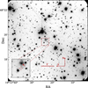 |
Fig. 4. Deep (1 h) r-band image taken with NOT+ALFOSC on 16 April 2023 (+313.1 d; Table A.1). A faint source is visible at the location of SN 2022lxg. Interestingly, a known galaxy (WISEA J191523.71+481938.5), |

3.2. Photometric analysis
3.2.1. Broadband light-curve evolution
In the following subsection, we present the features of the broadband light-curves of SN 2022lxg. These include the explosion epoch estimate, the peak epochs and magnitudes in the various bands, the rise and decline timescales, and the colour evolution.
The last non-detection (in the i band) was at MJD 59 730.45 while the first detection was at MJD 59 731.39 in the g band. Moreover, the first three detections (in ZTF g, r and ATLAS c bands) are within ∼ one day from the last non-detection (at 59 731.44 in r band and at 59 731.50 in c band). However, due to the very fast early rise and the very blue colours of SNe at epochs so close to the explosion, the i-band last non-detection is not particularly constraining. In order to determine the explosion epoch, we applied the following steps: The first estimates from the blackbody fits some days after these very early detections (> 2 d), return temperatures ∼20 000 K (see Sect. 3.2.2). However, right after the explosion (≲1 d), SNe temperatures can decline very rapidly from several 10 000 K (Yaron et al. 2017). Hence we assume a temperature of 40 000 K for these early epochs and using the flux densities in the various bands, we obtained an estimate of the radius (3.9 × 1013 cm, 7.0 × 1013 cm, 9.9 × 1013 cm respectively). Applying the Stefan-Boltzmann law yields the blackbody luminosities of these points and we propagated the uncertainties of the luminosities in the standard way. Given the inherent assumptions and systematic uncertainties in this process (especially since we do not have UV photometry to tightly constrain the early temperatures), we allowed for generous errors on the temperature (σT = 25 000 K) and radius (σR = 1014 cm). We fit a linear model to the obtained luminosities using a custom Monte Carlo routine with 10 000 iterations (and assuming uniform distributions for the priors), thereby retrieving a posterior distribution on when the fits cross the zero luminosity level (i.e. explosion epoch); we use the median of this distribution as the explosion epoch estimate, and the 16th and 84th percentiles as the explosion epoch uncertainties. The median fit is within 1σ from all the next, rising points (i.e. those not included in the fit), hence a linear model suffices for the purpose of estimating the explosion epoch. We find MJD and adopt this as our reference epoch throughout the manuscript. Therefore, the first g-band detection was made within ∼1 hour from the explosion.
In order to determine the epochs of maximum light in each of the optical bands, we performed numerical interpolation of the light-curves using a Gaussian process regression algorithm (Seeger 2004). We used the Python package GPy5, employing a radial basis function (RBF) kernel. The uncertainty in the peak epoch was estimated as the time range when the GP light-curve is brighter than the 1σ lower bound on the peak brightness. For the peak epochs of the three different bands (gri), we find MJD = 59 739.14 , 59 745.17
 and 59 746.26
 , respectively. We note a lag between the peak epochs with the bluer bands peaking earlier; 6.0 d between g and r, and 1.1 d between r and i. The peak epochs are denoted as short vertical dashes in the inset of Fig. 2 where we show the shape of the light-curves around this time and the GP interpolations that were employed to measure them. In terms of peak absolute magnitudes, we obtain Mg = −19.41 ± 0.01 mag, Mr = −19.31 ± 0.02 mag and Mi = −19.09 ± 0.02 mag respectively. This brightness makes SN 2022lxg a LSN, in between the SNe II and the superluminous SNe II (SLSNe-II). The photometric and spectroscopic properties of SN 2022lxg show remarkable similarities with those of the sample of LSNe Type II studied by P23. These properties will be highlighted further as we present and study the properties of SN 2022lxg.
The rest-frame rise time from explosion to peak in the g band is 7.6 ± 2.2 days (and 13.5 and 14.6 days in the r and i bands respectively), consistent with the median of Type II SNe (7.5 ± 0.3 d; González-Gaitán et al. 2015). During this time frame, it rose by 5.4 mags with a rate of 0.56 mag day−1. However, the rate considerably slows down close to the peak, and especially in the g band, there is a plateau of ∼8 days at ∼ − 19.38 mags that we mark with a horizontal dashed line in the inset of Fig. 2 (a linear fit to the plateau). That plateau is not seen in the r and i bands, the former however shows a ‘bump’ at those epochs, while the latter shows a smoother evolution around peak (see also discussion in Sect. 4.1.2). Hence, the fast rise can be better appreciated by measuring the same quantities from the first to the second g-band detection, where within ∼1.9 days the g band rose by 4.9 mags, a rate of 2.6 mag day−1. In order to account for this change in the slope of the rise and fairly compare to other SNe with different light-curve morphologies and tight explosion constraints, we follow the approach of Gall et al. (2015) where they define an epoch termed ‘end-of-rise’, as the epoch at which the r-band magnitude rises by less than 0.01 mag d−1. This is estimated by fitting a low-order polynomial to the data, with an iteratively chosen step-size in time. For the r- band, we measure the ‘end-of-rise’ at MJD 59 741.59 ± 1.73 (i.e. 10.00 d post explosion in rest-frame) with an absolute magnitude of −19.27 ± 0.10. In the left panel of Fig. 5, we plot the measured ‘end-of-rise’ time of SN 2022lxg in the r band versus the respective absolute magnitude at this epoch, and we compare those to the sample of Gall et al. (2015), a compilation of 23 Type II SNe of various subtypes. SN 2022lxg is the brightest of them with an intermediate ‘end-of-rise’ time.
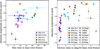 |
Fig. 5. Light-curve rise and decline timescales against absolute magnitude. Left: Rise time against the Gall et al. (2015) sample measured from the r band. The P23 sample does not have explosion constraints, and is therefore not included here. Right: Decline rate of SN 2022lxg (filled marker in g band, open marker in V band), compared to other luminous Type II SNe from the P23 sample (V band), the Type IIP/IIL sample of Faran et al. (2014) (V band), and several unusual transitional and/or interacting Type II SNe; SN 1996al (Benetti et al. 2016) (B band), SN 1998S (Leonard et al. 2000; Fassia et al. 2000) (V band), SN 2016gsd (Reynolds et al. 2020) (B band), SN 2017ivv (Gutiérrez et al. 2020) (V band), SN 2018ivc (Bostroem et al. 2020; Maeda et al. 2023a; Reguitti et al. 2024) (B band), and the fast and faint Type IIb SN SN 2020ikq (Ho et al. 2023) (g band). |
By 50 d from peak, SN 2022lxg has declined by 3.48 ± 0.26 mag (50 d)−1 in the g-band; it continued to decline at this rate until ∼ + 100 d (i.e. ∼6.96 mag (100 d)−1), when it became too faint for further observations. In order to compare with V-band literature measurements, we employed the following process: We obtained synthetic photometry in the g (ZTF) and V (Bessel) filters (using the filter curves hosted at the SVO Filter Profile Service; Rodrigo et al. 2012, 2024; Rodrigo & Solano 2020) from our dense spectral series. In order to retrieve the V-band magnitudes at the g-band light-curve epochs, we linearly interpolated the derived g − V synthetic colour curve. In that way we created a ‘transformed’ V-band light-curve and measured the decline rate to be 3.18 ± 0.33 mag (50 d)−1. The decline is significantly faster than the fastest declining (∼2.5 mag (50 d)−1). Type IIL SNe reported in Faran et al. (2014). Interestingly, the decline rate of SN 2022lxg is reminiscent of Type IIb SNe (5 − 9 mag (100 d)−1; e.g. Gutiérrez et al. 2020 and references therein). Up to an epoch of ∼100 d, the pseudo-bolometric luminosity of SN 2022lxg did not settle onto the expected decline rate for 56Co decay of 0.98 mag (100 day)−1 (assuming complete gamma-ray trapping; Woosley et al. 1989). Our attempt to obtain a late-time constraint at +261.3 d and subsequently at +313.1 d, resulted in a non-detection and an upper-limit of 22.96 mag, and in a detection of 24.00 ± 0.12 mag (Mr = −10.91 mag) respectively (Fig. 2). We searched for archival images that could be used as templates for difference imaging. However, the deepest image available is from the PanSTARRS1 survey (Kaiser et al. 2002); we measure a limiting magnitude of r ∼ +22.8 at the SN location. As this is significantly shallower than our deepest science image, we do not perform template subtraction. The late-time detection implies that the initial fast decline rate reported above must have slowed down, but it is difficult to firmly attribute the cause of this based on a single data point.
In the right panel of Fig. 5, we show the magnitude decline rate per 50 days versus the peak absolute magnitude. We compare with two samples: the Type IIP/IIL sample of Faran et al. (2014) and the one of P23 (both measure the decline rates from the V band). The latter are all characterised as fast declining. Here, similar to P23, we consider as fast, those SNe with decline rates ≳1.4 mag (100 d)−1, an arbitrary limit that has previously been used to separate slow and fast declining SNeII (Davis et al. 2019 and references therein). We also include several unusual transitional and/or interacting Type II SNe. The only SN from the P23 sample that declines faster than SN 2022lxg is SN 2017hxz. We show the morphology of the r/R-band light-curves (and few in the V-band) in Fig. 6 compared to brighter, slower declining Type II SNe, and fainter, rapidly declining ones. Although there is significant heterogeneity in the comparison objects, as we discuss below, SN 2022lxg has photometric and spectroscopic properties in common with both fainter and brighter Type II SNe.
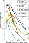 |
Fig. 6. Comparison of the absolute magnitude r-band light-curve of SN 2022lxg to three LSNe from the P23 sample in the V band (SN 2017cfo, SN 2017hbj, SN 2017hxz) and to other fast declining transients of various subtypes: SN 1998S, SN 2016gsd, SN 2018ivc in V band, and SN 1996al, SN 2020ikq, and two more Type IIb SNe (SN 2011dh; Arcavi et al. 2011; Bersten et al. 2012, SN 2011hs; Bufano et al. 2014) in the r/R band. Visual extinctions (for both MW and host galaxies) and distance moduli are retrieved from the referenced works (see also Fig. 5 for the references). There is a remarkable similarity in the decline rate (and luminosity) with SN 2017hxz of the P23 sample. |
Regarding the colour evolution, SN 2022lxg has rather blue colours (g − r ≲ −0.2 mag) for the first ∼10 days after the explosion, then until +40 days, the colours redden rapidly and reach a maximum value of g − r ∼ 0.6 mag. Then we see the cooling stop abruptly and the colour evolution plateaus, and even colours become slowly bluer until +65 d, followed by a more gradual cooling until the SN becomes too faint to observe. An almost identical colour evolution is seen in the P23 sample. We showcase this in Fig. 7 by reproducing their Figure 9 and including SN 2022lxg in the comparison as well as a few well-studied luminous SNe with similar colours, e.g. SNe 1998S and 1979C (Branch et al. 1981; de Vaucouleurs et al. 1981). In order to compare with B − V colours from the literature, we transformed these measurements to g − r using a procedure analogous to that described above for transforming to the V band. We plot the Gaussian process interpolations of the g − r and B − V light-curves (performed using the Python package GPy) and compare with the sample of P23, and also with the B − V colours of the sample of SNe II studied by de Jaeger et al. (2018). It is clear that SN 2022lxg follows the same pattern as the LSNe II of the P23 sample, and differs from the gradual cooling shown by the majority of Type II SNe. In Table 1, we tabulate various photometric properties of SN 2022lxg that were presented in this section.
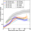 |
Fig. 7. Gaussian process interpolations of the colours (g − r in orange and B − V in blue) of SN 2022lxg compared to those of other luminous Type II SNe from the P23 sample. We overplot the actual measured g − r colours of SN 2022lxg with faint squares and the 1σ uncertainties of the interpolations as shaded lines. Mean values of B − V colours of the sample of SNe II studied by de Jaeger et al. (2018) are presented in grey for comparison (with the 1σ standard deviation plotted as a shaded region). |
3.2.2. Bolometric light-curve
We constructed a pseudo-bolometric light-curve of SN 2022lxg using SUPERBOL (Nicholl 2018). The flux in the available bandpasses was estimated at the epochs of our r-band photometry. We interpolate the light-curves using polynomials of third to fifth order and integrate under the spectral energy distribution (SED) of each epoch to get the luminosity. We fit a blackbody function to the SED at each reference epoch in order to estimate the temperature and the radius, and also to calculate the missing energy outside of the observed wavelength range. The pseudo-bolometric light-curve, as well as the blackbody temperature, radius and luminosity evolution are shown in Fig. 8. We note that the results should be interpreted with caution as we have photometric coverage for the full evolution of the SN in only five optical bands (gcroi) and only four points between +40 to +60 d in the z band; thus, the temperature estimates at early times are almost certainly underestimated. In the inset of the top panel of Fig. 8 we visualise how we estimated the explosion epoch (Sect. 3.2.1).
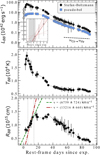 |
Fig. 8. Pseudo-bolometric gcroiz light-curve of SN 2022lxg (top panel) and blackbody temperature and radius evolution (middle and bottom panels) derived from blackbody fits to the SEDs. The bolometric luminosity derived with the Stefan-Boltzmann law is also shown in the top panel, with the open markers showing the luminosity estimates of the early first three detections (within three hours from the explosion), converted from temperature to luminosity using the Stefan-Boltzmann law. The inset zooms-in on those points where we plot in red ten random samples from the posterior distribution of linear Monte Carlo fits. The vertical grey line denotes the explosion epoch estimate (median of the posterior distribution) while the shaded grey region denotes the uncertainty on the estimate (16th and 84th percentiles). In the bottom panel, we show linear fits to the rising part of the expanding photosphere (the exact fitted region is within the vertical dotted lines), the dash-dotted red fit has R(t = 0) fixed at zero, while the dashed green one does not. |
The bolometric light-curve analysis results in a blackbody temperature that peaks at ∼20 000 K at 5 days post explosion. Then the temperature drops fast for the next 10 days, followed by a ∼10 day break in the cooling and then the cooling rate becomes fast again until +35 d. From Between roughly +35 to +75 d the cooling rate significantly drops and even plateaus, only to drop again until the SN becomes too faint to observe. The blackbody photosphere expands linearly until ∼ + 20 d, and a linear fit to this expansion results in an photospheric velocity of vph = 6759 ± 724 km s−1. Fixing R(t = 0) at zero, returns a higher velocity of vph = 13216 ± 660 km s−1 however the fit is not as good. Between +15 to +35 days, the radius almost plateaus, that is it slightly drops during the cooling rate break, and then peaks again at RBB ∼ 1.4 × 1015 cm, at the end of the second fast cooling phase. After that, the photosphere contracts until the SN becomes too faint to observe. The pseudo-bolometric luminosity slowly peaks at ∼7.2 × 1042 erg s−1 at 12 days post explosion and then smoothly declines. The luminosity derived from the Stefan–Boltzmann (SB) law follows a similar evolution, with a sharper peak of ∼6.4 × 1043 erg s−1 at 5 days post explosion.
Using the bolometric luminosity, we make some 56Ni mass estimates produced in SN 2022lxg. For H-rich SNe, it is very difficult to estimate how much of the power comes from nickel during the peak times when the hydrogen recombines, leading to inaccurate estimates. This also applies to SN 2022lxg; by plugging the above peak estimates into the Arnett rule (Arnett 1982), we measure 0.25 M⊙ and 1.21 M⊙ for the 56Ni mass, using the pseudo-bolometric and the SB estimate respectively. These values should be seen as rough upper-limits. Based on the colours of the SN before it faded, we construct a pseudo-SED for our late r-band detection at +313.1 d. From that, we measure a pseudo-bolometric luminosity of (1.7 ± 0.7)×1039 erg s−1, and from a blackbody fit and the Stefan–Boltzmann law, we get a luminosity of (6.2 ± 2.7)×1039 erg s−1. We use these to estimate the 56Ni mass from the tail of the luminosity using various prescriptions (Tail, Hamuy 2003, SN 1987A ratio) and we always measure values < 0.009 M⊙. Those values should be seen as a rough lower-limits since we do not have a good estimate of the bolometric luminosity at these epochs. The 56Ni masses estimated from the tail are very low, further highlighting that the estimates derived from the peak are not trustworthy and that the peak is not dominated by 56Ni-heating. We tabulate the median values of the above 56Ni mass estimates in Table 1, and all the individual values in Table A.3.
3.2.3. Light-curve fits
We used the publicly available Modular Open Source Fitter for Transients (MOSFiT6; Guillochon et al. 2018) to fit the multi-band light-curves. MOSFiT takes as input the multi-band photometry and priors on the parameters of the model that is being fit to the data. We used the built-in model csmni that combines the luminosity from the decay of radioactive 56Ni and additional luminosity from CSM interaction, wherein a fraction of the kinetic energy of the SN ejecta is converted to radiative energy through collision with the CSM. The 56Ni decay model is from Nadyozhin (1994), while the CSM interaction model is based on the semi-analytic treatment of Chatzopoulos et al. (2013). The model is set up such that the contribution from CSM interaction starts at time tint = R0/vej, where R0 is the inner radius of the CSM shell and vej is the bulk velocity of SN ejecta. Assuming vej to be the average photospheric velocity of the SN ejecta, the kinetic energy Ek of the ejecta is inferred from the free parameters Mej (the ejecta mass) and vej, assuming a constant density (Arnett 1982), using  . The model has 11 free parameters, namely 56Ni mass fraction (fNi ≡ MNi/Mej), γ-ray opacity (κγ), bulk velocity of SN ejecta (vej), mass of the CSM shell (MCSM), total ejecta mass (Mej), host galaxy hydrogen column density (nH, host), inner radius of the CSM shell (R0), CSM density at the initial radius R0 (ρ0), minimum temperature (Tmin) that the expanding and cooling photosphere settles down to, time of explosion relative to first epoch of observation (texp) and a white-noise variance term (σ) representing the additional uncertainty (in mag) that would make the reduced χ2 = 1. A power-law density profile for the CSM shell is adopted with ρ(r) = qr−s, where the scaling factor
  (Chatzopoulos et al. 2012). The power-law index was fixed to s = 2 corresponding to a steady-wind CSM model (Chevalier & Irwin 2011). Furthermore, there are three more parameters that we fix; the Thomson scattering opacity (κ) at 0.34 cm2 g−1, a typical value for hydrogen-rich ejecta (close to the result of Nagy 2018), and the density power-law parameters in the inner (ρej ∝ r−δ) and outer (ρej ∝ r−n) ejecta, δ = 0 and n = 12, respectively (typical values in H-rich ejecta; Chatzopoulos et al. 2013).
We set simple uninformative uniform or log-uniform priors for each free parameter of the model. We set a well-constrained uniform explosion time prior (texp > −1) since we have put tight constraints on the explosion time and we also use the last non-detections for the fits. We also set a uniform velocity prior around our estimate of 20 000 km s−1 (from the minima of absorption lines; see Sect. 3.3): between 17 000 and 23 000 km s−1. Based on the lack of narrow Na I D absorption lines in the spectra and the very faint (potential) host, we also set an upper limit for the host galaxy extinction, AV, host ≤ 0.5 mag, converted from the column density of neutral hydrogen as nH, host ≤ 1021 cm−2 based on Güver & Özel (2009). We also have a good constraint on the Tmin from the blackbody fits, and we set a prior between 5000 and 8000 K. Finally, we assume a hydrogen-rich progenitor, but not necessarily an extended envelope such as that of a red supergiant (RSG). Thus the minimum inner radius of the CSM, R0, is set at 0.1 AU (∼20 R⊙), roughly half the radius of the blue supergiant progenitor of SN 1987A (Podsiadlowski 1992) but larger than a Wolf-Rayet progenitor of a stripped-envelope (SE) SN.
We ran MOSFiT using dynamic nested sampling with DYNESTY7 (Speagle 2020) in order to evaluate the posterior distributions of the model. We list the free parameters of the model, their priors and their posterior probability distributions in Table 2, and we present the model light-curves in Fig. 9, with two-dimensional posteriors shown in Fig. B.1 of the Appendix. The fit has fully converged with well-constrained parameters and the logarithm of the Bayesian evidence Z (which quantifies the quality of the fit) is equal to log(Z) = 191. The model is successful in reproducing the multi-band light-curves. The only deviation is that the model light-curves return a sharper peak (in all bands) than the smoother peaks of the data. Finally, the r-band model light-curves successfully fit the late-time, deep r-band epoch (+313.1 d).
Priors and marginalised posteriors for the MOSFiT csmni model.
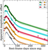 |
Fig. 9. Fits to the multi-band light-curve using the csmni model in MOSFiT (Guillochon et al. 2018). The relevant parameters are listed in Table 2. |
Some key explosion parameters are:  a very low fraction of which (∼1%) is 56Ni (
 ; within 1σ from our SB tail estimates), and
  km s−1, which combined with the ejecta mass leads to
  erg. The very low 56Ni mass and the high ejecta velocity are fully consistent with the results derived from other observables. However, the ejecta velocity of the model (that fully agrees with what we derive from the spectroscopic lines; see Sect. 3.3) is much higher compared to the rather low photospheric expansion velocity derived from the blackbody fits (∼7000 km s−1). This discrepancy is further discussed in Sect. 4.2. The very low ejecta mass could be somewhat under-estimated; however, a broadly low ejecta mass is consistent with the fast nature of SN 2022lxg and with the lack of typical metal lines in the spectra (see Sect. 3.3). Some key CSM parameters are
  , with an inner CSM radius and density of
  cm (∼1.38 AU) and
  g cm−3 respectively. In order to reproduce the fast evolution and luminous peak of SN 2022lxg, the model favours a low-mass, dense CSM close to the progenitor, blasted by the low-mass, fast-moving ejecta. The inner CSM radius R0 can put an upper-limit on the radius of the progenitor (R⋆ ≲ 297 R⊙). The high density and low mass of the CSM implies that it occupies a small volume (i.e. not extended). The ejecta interact with the CSM immediately after explosion (tint ∼ 2.9 h after explosion), and due to the small volume of the CSM, the fast ejecta sweep it up quickly. If indeed the CSM is that dense, that could explain why the evolution of the light-curves slows down around the peak epochs (even showing a small plateau around peak in g band; see Sect. 3.2.1), but then the light-curves decline rapidly. Finally, the model predicts a negligible host extinction and sets the explosion epoch at MJD
 within 3σ from our estimate.
We note here several caveats of the model fits above. Concerning the CSM configuration, the Chatzopoulos et al. (2013) model assumes optically thick interaction that would not be appropriate for low CSM masses. Additionally, regardless of what the value of s, the power-law index (e.g. s = 2 for a wind-like CSM and s = 0 for a shell of constant density), the CSM is assumed spherically symmetric cf. Sect. 3.4. Another caveat is that the γ-ray opacity (κγ) is a free parameter with a higher prior up to 10. However, this value is usually assumed fixed at 0.027 cm2 g−1 (e.g. Cappellaro et al. 1997). Our best model fit returns a value of 3.4 cm2 g−1. If we fix this value to 0.027, the model under-fits the late-time r-band detection by ∼ an order of magnitude and suggests that the interaction with the CSM starts ∼2 d after explosion, which is at odds with the observations. In order to assess the influence of κγ and our last detection (+313.1 d) of the SN, we recomputed the fits with κγ fixed to 0.027 cm2 g−1 and excluding the +313.1 d data point. We find mostly similar values for the ejecta and CSM parameters, but with an order of magnitude higher 56Ni mass. Overall, the fit fails to match the rise or peak magnitude in any band, and for some bands the decline as well. It is possible that weak ongoing CSM interaction that is not accounted for by MOSFiT is manifested as an increased value of κγ. Furthermore, we tried several configurations for the s, d, and n parameters but the fit that we present in this section is the best (in terms of log(Z) but also in capturing the photometric evolution both at early and late times). We also tried relaxing the ejecta velocity priors (e.g. setting the minimum to 5000 km s−1) consistently returns velocities between 17 000 and 23 000 km s−1. Finally, we also tried individually the default model (luminosity powered only by the decay of radioactive 56Ni) and the csm model (luminosity powered only by interaction) and both models returned bad fits, both in terms of log(Z) and fitting the data points, but also by returning unphysically high 56Ni masses (the former) or very low ejecta masses (∼0.5 M⊙) the latter. All the above considered, the model fit results should be interpreted with caution and the struggle of different configuration to explain the data might be a hint that the CSM is indeed non-spherical.
3.3. Spectroscopic analysis
3.3.1. Early spectra and flash-ionisation features
Our earliest spectrum (+2.20 d, left panel of Fig. 10) shows flash features on top of a ∼18 000 K continuum that we attribute to Hα, Hβ, Hγ and He IIλ4686. We simultaneously fit Lorentzian and Gaussian profiles to account for the narrow and underlying broad components, respectively. For Hα we find a FWHM of 241 ± 19 km s−1 and 2814 ± 228 km s−1. For the He II features, we find 226 ± 37 km s−1 and 3717 ± 356 km s−1, while for Hβ we find 389 ± 65 km s−1 and 3829 ± 1014 km s−1. A narrow component around Hα appears in some of the later spectra, but at the resolution of our spectra, we cannot determine whether this is due to underlying emission from an H II region. As shown in the continuum subtracted spectra in right hand panel of Fig. 10, the flash features persist out to ∼8 d. The two subsequent spectra (+8.66 and +9.67 d) are of too low a spectral resolution to detect weak narrow features, but by the epoch of our next spectrum (15.45 d), there is no sign of He II. We therefore conclude that the flash-ionisation lines must have disappeared by ∼ + (8 − 9) d. Following Bruch et al. (2023), we calculate the flash timescale as the time from the estimated explosion date to the mid-point between the last spectrum that shows the He IIλ4686 line and the first one that does. Choosing our +8.66 d spectrum as the latter, leads to a timescale of 8.24 ± 0.42 days, while being more conservative and choosing our +15.45 d spectrum, gives 11.63 ± 3.82 days. Both values are in agreement with Bruch et al. (2023) who argue that the duration of the flash-ionisation features is partially correlated with the rise time and the absolute peak magnitude. We show the location of SN 2022lxg with their sample in Fig. B.2.
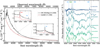 |
Fig. 10. Flash-ionisation features in SN 2022lxg. Left: Keck+LRIS spectrum, +2.20 d after the explosion. We see flash-ionisation lines of Hα, Hβ, Hγ, and He IIλ4686, on top of a blue continuum. The red spectrum below is a model from Dessart & Jacobson-Galán (2023) (‘mdot1em3early_nb5’) with a steady pre-explosion wind of 1 × 10⁻³ M⊙ yr−1 that successfully reproduces the early continuum shape and the flash-ionisation lines. The insets focus on the flash-ionisation lines of Hβ and He II (left inset) and of Hα (right inset), with the dashed vertical lines denoting the rest wavelengths of those lines. Right: Early, continuum-subtracted spectra of SN 2022lxg. Flash-ionisation lines are marked with dashed vertical lines. From left to right, we detect Hγ, He II, Hβ, and Hα. The spectra (apart from the LRIS one) are binned to 12 Å for visual purposes. The horizontal dashed lines denote the zero flux level of each spectrum after the approximate continuum removal. The telluric features are marked with shaded, vertical grey lines. |
3.3.2. Spectral evolution and line identification
After ∼10 d broad, shallow line profiles develop and become increasingly prominent as the continuum cools. The Balmer lines and the Ca II NIR triplet (λλ 8498.02, 8542.09, 8662.14) can be easily identified (Fig. 3). A feature close to He Iλ5876 and the Na I D doublet is also present. If it were solely due to He Iλ5876, then it appears red-shifted by ∼3000 km s−1. We would expect Na I D in emission to typically emerge at later epochs; attempting to de-blend the feature with two Gaussian profiles results in any contribution due to Na I D being red-shifted by ∼5000 km s−1. Hence, we conclude that it most likely is He Iλ5876 emission. There is also a broad feature around 5400 Å that we tentatively identify as Fe II (λλ 5169, 5267, 5363) and a blend of lines around and blue-wards the rest wavelength of Hβ. Both the He I and Fe II features appear to be strongest in the +41.73 d spectrum before gradually fading. We used the tools SNID (Blondin & Tonry 2007) and GELATO (Harutyunyan et al. 2008) to search for objects with spectra similar to those of SN 2022lxg during these early and intermediate phases (≲ + 45 d). The returned matches are of a range of SN subtypes and epochs, and therefore inconclusive. Nevertheless, a reasonable match is with the type IIb SN 2011fu (Morales-Garoffolo et al. 2015). Interestingly, these tools also return matches with some Type Ic SNe with broad spectral features (SNe Ic-BL). Some examples are SN 2013dx (D’Elia et al. 2015), SN 2007ru (Sahu et al. 2009) and SN 1998bw (e.g. Kulkarni et al. 1998; Woosley et al. 1999; Patat et al. 2001).
From about ≳ + 45 d, most features begin to fade with the exception of Hα and the Ca II NIR triplet. The He Iλ5876 feature, though weak, is still present in our last spectrum. We defer a discussion of the evolution of the Hα line to the next Section 3.3.3, but note that it displays a persistent blueshift until ∼ + 55 d after which it remains close to its rest wavelength, and gradually becomes narrower. In Fig. 11 we show the evolution of Hα, Hβ, and the Ca II NIR triplet in velocity space. The latter shows a P-Cygni profile, with the absorption minimum found at ∼20 000 km s−1, extending up to ∼24 000 km s−1. We note that for the epochs ≳ + 45 d, we start to see a break in the continuum around 5700 Å, with the continuum becoming suddenly stronger blue-wards of that wavelength. We again tried to find spectral matches to these epochs of SN 2022lxg using the aforementioned tools and get matches with SNe Type IIn. For epochs between +45 to +60 d where there is still He Iλ5876 in the spectra, we get good matches with SN 1996al (Benetti et al. 2016). After that, when Hα dominates the spectrum, we get good matches with SN 2005ip (Smith et al. 2009; Stritzinger et al. 2012). Indeed, the properties of SN 2022lxg share similarities with transitional complex SNe like SN 1996al (Type IIn/IIL; Benetti et al. 2016) and SN 2018ivc (Type IIb/IIL; Bostroem et al. 2020; Maeda et al. 2023a,b; Reguitti et al. 2024). They are fast rising and fast linearly declining (at least during their early < + 150 d evolution, see Fig. 6), with strong Hα emission as well as a prominent feature likely due to He Iλ5876.
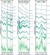 |
Fig. 11. Evolution of optical spectroscopic lines in velocity space. Left: Region around Hα. Note that for the epochs ≳ + 45 d, we seem to see a break around 5700 Å, with the continuum becoming suddenly stronger blue-wards of that wavelength. Middle: Region around Hβ. Right: Region around Ca II NIR triplet (centred on the middle line but all three lines are shown). The spectra are binned to 5 Å for visual purposes and the original spectra are plotted with lighter colours in the background. The dashed vertical grey line shows the central wavelength. The colours of the vertical lines denote the different elements, green is for helium and black for iron. Although only He Iλ5876 is robustly identified, we mark other helium lines to guide the eye. The telluric features are marked with shaded vertical grey lines. |
Allowing a free range in choice of epoch, we can also find superficial matches with bright, slowly declining Type II SNe. For instance the +103 d and +200 d spectra of SNe 1998S and 2021irp (Fassia et al. 2000; Reynolds et al. 2025a, respectively) bear some similarity to the +65 d spectrum of SN 2022lxg possibly indicative of similar ejecta or CSM conditions at those epochs. From the previous discussion on the light-curve and spectral evolution, it is clear that SN 2022lxg shares some properties in common with all Type II SN sub-groups. However, it consistently shares most properties in common mainly with the sample of objects in P23. Therefore, in what follows, we restrict our comparisons primarily to this group, but invoke analogous behaviour for a small handful of other SNe for illustrative purposes.
The spectral evolution of SN 2022lxg is also noteworthy in that typical metal lines seen in Type II SNe are conspicuous by their absence. The broad feature that we attributed to Fe II (λλ5169, 5267, 5363) is an exception. It is likely that our last spectrum (∼80 d) does not probe the nebular phase. Nevertheless, this lack of metal lines in the photospheric phase is another feature in common with P23. Another is a persistent emission line at ∼5800 Å, identified as He Iλ5876. The similarities between the Hα profiles will be discussed in detail in Sect. 3.3.3. In Fig. 12, we plot the spectral evolution of SN 2022lxg compared to LSNe II of the P23 sample, in order to highlight the spectral similarities throughout the different phases of the evolution of those SNe.
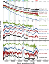 |
Fig. 12. Spectral comparison of SN 2022lxg to other luminous Type II SNe from P23, at different epochs. Emission lines are marked with vertical dashed lines. Although only He Iλ5876 is robustly identified, we mark other helium lines to guide the eye. There is a clear resemblance between SN 2022lxg and the comparison SNe throughout different phases. SN 2017cfo in particular appears to be the best match. |
3.3.3. Hα properties
Even during the flash-ionisation phase (≲ + 8 d), there is a broad shallow Hα component underneath the narrow feature. The profile broadens quickly and gradually becomes stronger. The LSNe II in the P23 sample show a weak or non-existent absorption component in their Hα profile (i.e. a P-Cygni profile). Similarly, the Hα profile of SN 2022lxg only shows a weak absorption component, more evident at the +15.45 d spectrum, that appears even weaker as the SN evolves, probably due to contamination from the strong He Iλ5876 emission. In studies of Type IIP SNe, a weak or absent absorption component associated with the Hα profile correlates brighter peak magnitudes, fast decline rates, and high velocities (Gutiérrez et al. 2014), similar to what we observe for SN 2022lxg. As it evolves, the Hα emission profile shows a blue excess, and a bump on its red side, coincident with the wavelength of He Iλ6678. Blue-shifted emission peaks are indeed expected in Type II SNe (Anderson et al. 2014b). At ≳ + 55 d the profile narrows down and becomes centred to the rest wavelength, while the red bump completely disappears. We performed a spectroscopic line study in order to quantify the properties of the Hα line using customized Python scripts. For this study, we use all our eight NOT+ALFOSC spectra that ensure consistency between the measurements and a good sampling of the evolution of the event from explosion to fading. Additionally, we include our first Keck+LRIS spectrum (+2.20 d). For all the following measurements, we remove the (linear) continuum locally. We quantify the line luminosity and the pseudo-equivalent width (pEW) by integrating under the line profile. In order to measure the velocity width (FWHM) we used a custom script in Python which first smooths the spectrum, then locates the data points on the left and right of the maximum that have flux values closest to the half of the maximum and then calculates the distance between them on the x-axis. The observed central wavelength of the line is defined as the middle point of this distance, and its distance from the central wavelength of Hα is defined as the line offset. We use a custom Monte Carlo method (10 000 iterations of re-sampling the data assuming Gaussian error distribution) in order to calculate uncertainties for the flux (luminosity), line width and offset from the central wavelength.
In the sub-panels of Fig. 13, we present the Hα luminosity (top panel), pEW (second panel), velocity width (third panel) and offset from the rest wavelength (bottom panel), of SN 2022lxg. We find that the luminosity of the line is quickly rising until it peaks at ∼ + 36 d with a luminosity of ∼5.5 × 1040 erg s−1. After that, it declines with a slower pace, measuring a luminosity of ∼2.0 × 1040 erg s−1 in our last spectrum (+79.96 d). The pEW very slowly rises until the intermediate epochs (∼ + 36 d) and then it sharply rises. Since the pEW provides an indication of how strong the line is with respect to the underlying continuum, what we observe in SN 2022lxg is that, even though the luminosity of Hα drops after ∼ + 36 d, the luminosity of the continuum drops much faster. This is not surprising since we have already highlighted how fast the light-curves of SN 2022lxg decline. The velocity width (FWHM) and offset of the line, indeed evolves like the LSNe II in the P23 sample. The FWHM quickly (∼ + 10 d) rises to values around 10 000 km s−1 and then more slowly reaches its peak at ∼15 000 km s−1 in the same epoch that the luminosity peaks. Similarly, the velocity offset reaches a blueshift of ∼ − 1000 km s−1 during the epochs that the line luminosity and FWHM peaks, before it gradually gets centred to the rest wavelength of Hα. There is one epoch (first NOT+ALFOSC spectrum at +5.53 d) where the broad shallow profile seems to broaden too fast (a jump of ∼8000 km s−1 within ∼3.5 days) and the offset reaches ∼ − 2000 km s−1. The offset drops down to ∼350 km s−1 almost ten days after, and then smoothly reaches the local blueshift minimum at ∼ + 36 d. This same profile is seen in the +6.98 d UH88+SNIFS spectrum, giving further confidence that this is not instrumental/artefact, but a real feature of the SN. The rapid light-curve rise of SN 2022lxg, can potentially explain the fast evolution of the line profiles as well.
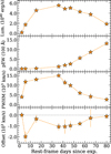 |
Fig. 13. Luminosity, pEW, FWHM, and velocity offset evolution of the Hα line emission. |
In Fig. 14, we present a direct comparison of the aforementioned Hα properties of SN 2022lxg with those measured in the spectra of the LSNe in P23. In the top panel we present the velocity width (FWHM) evolution (including available measurements of SN 2018ivc) while in the bottom panel we present the pEW evolution. For comparison, we also plot mean values for regular SNe II from the sample of Gutiérrez et al. (2017). The similarity between the evolution of both the FWHM and pEW of SN 2022lxg, with those of the P23 sample is striking. Combined with the fact that the velocity offset in their sample shows the same behaviour as the one of SN 2022lxg (most likely without the ‘spike’ at +6 d though), and with the fact that they show a tentatively identified He Iλ5876 as well as a clear lack of metal lines, leads to the conclusion that the events are spectroscopically similar.
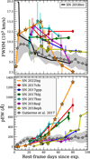 |
Fig. 14. Hα line emission FWHM (top) and pseudo-equivalent width (bottom) compared to other luminous Type II SNe from the P23 sample (adapted from P23). Mean values for regular SNe II from the sample of Gutiérrez et al. (2017) are presented in grey (with the 1σ standard deviation plotted as a shaded region). In the top panel, we also plot the Hα FWHM of SN 2018ivc (from Bostroem et al. 2020). |
3.3.4. Near-infrared spectroscopy
We present four publicly available near-infrared (NIR) spectra of SN 2022lxg in Fig. 15. The spectra were presented as part of the Keck Infrared Transient Survey (Tinyanont et al. 2024) and we collected them from the Weizmann Interactive Supernova data REPository (WISeREP8; Yaron & Gal-Yam 2012). The spectra are taken at phases +8 d, +23 d, +40 d, and +50 d. The first spectrum is practically featureless and blue, in accordance with the optical spectra at that time. In the second spectrum, a broad P-Cygni profile of He I 1.0830 μm line is formed, again in accordance with the optical when the He Iλ5876 line is emerging. In the last two epochs of +40 d, and +50 d, the main difference that we see in the NIR spectra is that hydrogen lines have emerged, again in accordance with the optical. We clearly detect strong Paβ but unfortunately Paα is blended with a strong telluric line. The He I 1.0830 μm line has become much stronger and is blended with Paγ, and in the last spectrum we also detect He I 2.0581 μm which is also blended with Brγ. In Fig. 16, we visualise in velocity space, the comparison of these last two spectra with the optical spectra at similar epochs (left panel) and between the two helium NIR lines (right panel). The absorption minimum of the He I 1.0830 μm P-Cygni profile lies at ∼20 000 km s−1 and extends up to ∼23 000 km s−1. That is fully consistent for what we find from the P-Cygni profiles of the Ca II NIR triplet and it also agrees with the FWHM of the Hα emission around the same epochs. All the above considered, we assume an ejecta velocity of ∼20 000 km s−1 for SN 2022lxg.
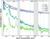 |
Fig. 15. NIR spectra of SN 2022lxg taken from Tinyanont et al. (2024). The spectra are binned to 5 Å for visual purposes and the original spectra are plotted with lighter colours in the background. The colours of the vertical lines denote the different elements; green is for helium and cyan for hydrogen. The tentatively identified magnesium and carbon are marked with black and red respectively (with a question mark next to the element name). The telluric features are marked with shaded grey regions. |
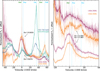 |
Fig. 16. Evolution of NIR spectroscopic lines in velocity space. The spectra are binned to 5 Å for visual purposes and the original spectra are plotted with lighter colours in the background. The vertical grey line shows the central wavelength. The colours of the vertical lines denote the different elements; green is for helium and cyan for hydrogen. Left: Optical (blue/green colour map) and NIR (red/orange colour map) spectra, centred at He Iλ5876 and λ10830, respectively. The spectra are normalised at ∼16 000 km s−1 red-wards of the central wavelengths. Dashed vertical lines mark elements in the optical while dashed-dotted ones mark elements in the NIR. Right: Evolution of He Iλ10830 (bottom) and He Iλ20581 (top) region of the spectra in velocity space. Dashed vertical lines mark elements in the top spectra while dash-dotted ones mark elements in the bottom ones. Both He I lines show multi-component profiles with absorption components at ∼ − 10 000 and −20 000 km s−1. |
Finally, in the last two spectra, there is an emission line at ∼1.82 μm that we identify as Mg I 1.183 μm, and a line at ∼1.65 μm that we tentatively identify as Mg II 1.680 μm. However, there is no sign of Mg I 1.504 μm in the spectra. There also seem to be two lines at ∼1.455 μm and 1.965 μm that are harder to identify. Using the National Institute of Standards and Technology (NIST) database9, we find two strong C I transitions close to these wavelengths that we mark with a question mark in Fig. 15. We do the same with the magnesium lines in order to highlight that all these lines are tentatively identified.
Another feature revealed by the NIR spectra, is the presence of a narrow P-Cygni profile at the peak of the emission of the He I 1.0830 μm line, at +40 and +50 days. Such profiles are often detected in spectra of interacting supernovae provided that they are of sufficient resolution. This points to unshocked CSM along our line of sight (e.g. Smith et al. 2002a; Kotak et al. 2004; Trundle et al. 2008; Andrews et al. 2025). We fit two Gaussian profiles to the absorption and emission components and measure a peak-to-peak offset between the two of 143.4 ± 3.8 and 150.9 ± 4.2 km s−1 respectively, which is larger than the instrumental resolution of Keck+NIRES (≈100 km s−1). The mixed H and He CSM suggests partial stripping of the progenitor. We searched for similar profiles in other lines (Fig. 17) and tentatively identify an absorption component in the Paβ line during the same epochs as for the He I 1.0830 μm line. Although our optical spectra are of too low a spectral resolution to draw robust conclusions, there may be hints of an absorption trough (Fig. 17) if we are guided by the near-IR spectra.
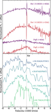 |
Fig. 17. Narrow P-Cygni profiles in velocity space. Top (LRIS NIR spectra): The two upper spectra clearly show narrow P-Cygni profiles of He I 1.0830 μm with peak to peak separations of ∼150 km s−1, pointing to unshocked CSM. In the two lower (same epoch) spectra, a narrow profile in the Paβ line is tentatively detected. Bottom: Four low-resolution optical spectra centred on Hα spanning ∼10 days. |
3.4. Polarimetric analysis
The intensity-normalised Stokes parameters (q = Q/I and u = U/I, where Q and U are the differences in flux with electric field oscillating in two perpendicular directions, and I is the total flux) were used to calculate the polarisation degree ( ), and the polarisation angle (χ = 0.5arctan(u/q)). All values of p presented in this paper have been corrected for polarisation bias (e.g. Simmons & Stewart 1985; Wang et al. 1997) following Plaszczynski et al. (2014).
We have measurements in the V and R bands for two epochs, +17.4 d and +36.1 d. We present the Stokes q − u planes for the imaging polarimetry results in Fig. 18 where we also plot the ISP estimate as a grey star. The measured values can be found in Table A.4. For the first epoch, we measure p = (1.04 ± 0.24)% and p = (0.79 ± 0.23)% for the V and R band respectively, and a polarisation angle of χ = ( − 25.92 ± 6.44)° and χ = ( − 33.90 ± 8.03)°. For the second epoch, we measure p = (0.65 ± 0.55)% and p = (0.46 ± 0.50)% for the V and R band respectively, and a polarisation angle of χ = ( − 28.85 ± 19.45)° and χ = ( − 4.01 ± 22.55)°. The accuracy of the second epoch measurements are low (p/σp ∼ 1), however the first epoch measurements are statistically significant (p/σp ∼ 3 − 4) and we measure polarisation of p ∼ (0.8 − 1)%.
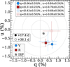 |
Fig. 18. Intensity-normalised Stokes q and u parameters, from ALFOSC imaging polarimetry, in the V (blue circles) and R (red squares) bands, at phases +17.4 d (filled markers) and +36.1 d (open markers). The grey star marks our best ISP estimate and the dashed circles mark the 0.5%, 1.0%, and 1.5% polarisation values (p). The first epoch (with a robust S/N ∼ 300) shows that SN 2022lxg is intrinsically polarised. |
In order to estimate the intrinsic polarisation of a source, the effect of the interstellar polarisation (ISP), introduced by dust grains in the line of sight, has to be estimated. Since the (potential) host galaxy is very faint and distant from the SN, we consider its contamination in the polarisation negligible. Hence we only treat contamination from the MW. SN 2022lxg lies in a crowded field with many stars, so we can put tight constraints on the MW ISP. For each filter, we make a weighted average estimate between the field stars within each epoch and then double confirm with the ISP estimate of the other epoch. We measure qISP = (0.19 ± 0.05)% and uISP = ( − 0.23 ± 0.05)% leading to pISP = (0.29 ± 0.05)% and χISP = ( − 25.75 ± 4.92)°. Another way to roughly estimate an upper-limit for the Galactic ISP is with the empirical law 9 × E(B − V)% (Serkowski et al. 1975), and for SN 2022lxg that would be ∼0.53%, consistent with our estimate. We also checked for polarisation standard stars published in Heiles (2000) that are close to the location of SN 2022lxg. We find one star within 3.5° from the location of the SN with a polarisation value of p = (0.0 ± 0.2)%, again consistent with the above estimate.
We perform vector subtraction in the q − u plane in order to remove the ISP contribution and estimate the intrinsic polarisation of SN 2022lxg. In Fig. B.3 of the Appendix, we present the ISP subtracted Stokes q − u planes for the imaging polarimetry results. For the first epoch, we measure p = (0.73 ± 0.25)% and p = (0.49 ± 0.24)% for the V and R band respectively, and a polarisation angle of χ = ( − 25.99 ± 5.9)° and χ = ( − 38.35 ± 12.47)°. For the second epoch, we measure p = (0.34 ± 0.55)% and p = (0.30 ± 0.51)% for the V and R band respectively, and a polarisation angle of χ = ( − 30.66 ± 31.00)° and χ = ( − 8.92 ± 31.06)°. The polarisation values in the first epoch (with a robust S/N ∼ 300) suggest a mildly aspherical configuration (ellipticity of b/a ∼ 0.85; Hoflich 1991). There seems to be an evolution towards a more spherical configuration although the S/N of the second epoch is not optimal (∼150) and we cannot draw robust conclusions from those measurements.
4. Discussion
In the previous sections, we presented the optical and NIR properties of SN 2022lxg. We now attempt to piece them together to place SN 2022lxg in the context of other luminous Type II SNe, with a view to shedding light on its progenitor system.
4.1. The nature of SN 2022lxg
4.1.1. CSM interaction
There are several features in the data of SN 2022lxg that point to the fact that interaction between the ejecta and the CSM is the primary energy source for a large part of its evolution. Concerning the early phase, the very fast rise and the luminous (V ≲ −18.5 mag) peak of Type II SNe are usually attributed to such an ejecta/CSM interaction, where the kinetic energy of the ejecta is thermalised by the interaction shock and then radiated (see e.g. Moriya & Tominaga 2012; Andrews & Smith 2018; P23). The flash-ionisation lines are also a clear spectroscopic indication (Gal-Yam et al. 2014; Shivvers et al. 2015; Yaron et al. 2017; Dessart et al. 2017; Bruch et al. 2021, 2023; Jacobson-Galán et al. 2024), along with the blue featureless continua (confirmed by the early blue colours), as shocks produced during the interaction of the fast moving ejecta with the CSM heat the material. The broad-boxy profiles of Hα is another signature (Dessart & Hillier 2022). Furthermore, the blue pseudo-continuum observed (blue-wards of 5700 Å in this case) after ≳ + 45 d, has been attributed to a forest of blended Fe II lines provided by fluorescence in the inner wind or post-shock gas (Foley et al. 2007; Chugai 2009; Smith et al. 2009; Pastorello et al. 2015; Perley et al. 2022), and its presence here suggests that CSM interaction is ongoing.
Dessart & Jacobson-Galán (2023) considered a solar-metallicity 15 M⊙ red supergiant exploding into circumstellar material, and provide a grid of synthetic spectra resulting from different initial parameters such as the CSM density and the progenitor’s mass-loss rate. Although both the progenitor and explosion properties are likely to be different for SN 2022lxg, as the authors note, this would introduce only moderate variations and the overall conclusions presented should hold at a qualitative level. We attempted to find a match within this grid by focussing on our earliest spectrum (+2.20 d), that contains the flash features. We found one model that provided an adequate match to these lines ‘mdot1em3early_nb5’, a standard RSG star embedded in a steady-state wind with a mass-loss rate of 1 × 10⁻³ M⊙ yr−1, 1.25 days after the shock breakout (with a CSM velocity of 50 km s−1). However, the model lacks the broad wings that we observe in the data, and shows P-Cygni profiles that we do not detect. We show the comparison in Fig. 10.
During the phases between +15 to +40 d, the colours redden quickly. However, around +40 d several important changes seem to happen. The photosphere starts receding (see bottom panel of Fig. 8) and we see the cooling stop abruptly and the colours reach a plateau before slowly become bluer until +65 d when cooling seems to take over again through to the end of our spectroscopic coverage. Spectroscopically, the Hα luminosity and FWHM start to decline (first and third panel of Fig. 13) and the He I and Fe II lines start to fade as well. This is probably the result of the photosphere receding as the ejecta expand. As the temperature drops and the optical depth in the ejecta decreases, we start to see increasing emission from the CSM component and less from the ejecta. It is no surprise then, that this is when we see interaction dominate once again the colours (plateauing) and the spectra, most evident in the latter as Hα becomes the most prominent line in the spectrum. Even though the luminosity of Hα starts to decline after +40 d, it declines slower than the continuum, which explains the sudden rise in the pEW (bottom panel of Fig. 14). Also the velocity of Hα decreases due to interaction taking over. We also observe similar behaviour in the NIR hydrogen lines, where Paβ clearly emerges in the +40 d spectrum, but within ten days it becomes narrower and stronger with respect to the continuum.
4.1.2. Similarities with transitional Type II SNe
As discussed in Sect. 3.3.2, during the first ∼15 days, we see a blue continuum, featureless or with very shallow broad lines, a result of the shock heated and shock ionised CSM. After that, the continuum starts cooling, hydrogen recombines and we start to see spectral lines likely originating in the ejecta. Along with the Balmer series, we also see strong He Iλ5876 and Fe II (λλ 5169, 5267, 5363), appearing at the same phases and with similar shapes and FWHM (∼10 000−15 000 km s−1) as Hα. This is evidence that all these lines are coming from the ejecta and not from the interaction with the CSM, which means that the ejecta contain both hydrogen and helium. Furthermore, the evolution of those lines and the emergence of the narrower, strong Hα at later times (≳ + 35 d) together with slow moving (∼150 km s−1) helium suggests that the progenitor has undergone a degree of stripping of its outer layers.
This is reminiscent of a Type IIb SN (cf. Sect. 3.3.2) so we investigate whether there is further resemblance to transitional Type II SNe. In Fig. 19 we compare SN 2022lxg to Type IIb SNe, at different phases. We find a clear similarity with various SNe IIb, both in the early phases (∼ + 15 d) and more so in the subsequent ones (between +15 to +35 d), where the ejecta lines have clearly emerged. As the optical depth of the ejecta drops and the photosphere recedes around +40 d (see bottom panel of Fig. 8), the interaction with the CSM becomes dominant (≳ + 35 d onwards) leading to a spectroscopic change from a SN IIb, to spectra that resemble more an interacting SN II.
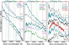 |
Fig. 19. Spectral comparison of SN 2022lxg to other Type IIb SNe throughout different phases of its evolution. Left: ≲16 d, middle: between ∼(16 − 36) d, right: ≳36 d. The y-axis in the left and middle panel is in log-scale while in the right panel it is linear. Emission lines are marked with vertical dashed lines. There is a clear resemblance between spectra of Type IIb SNe and those of SN 2022lxg throughout different phases of its evolution. |
There are questions arising from the apparent similarity with Type IIb SNe. We do not see two peaks in the light-curves typical in many SNe IIb, with the second peak occurring around three weeks after the first (SN 1993J; Filippenko et al. 1993; Wheeler et al. 1993; Richmond et al. 1994; Woosley et al. 1994, SN 2011dh; Arcavi et al. 2011; Bersten et al. 2012; Ergon et al. 2015, SN 2011fu; Morales-Garoffolo et al. 2015, SN 2011hs; Bufano et al. 2014, SN 2013df; Morales-Garoffolo et al. 2014), although there are SN IIb that do not show two distinct peaks (e.g. SN 2008ax; Roming et al. 2009, SN 2020acat; Medler et al. 2022). A lack of the first shock breakout cooling peak, implies that the progenitor must have been relatively compact. The first luminous peak is thought to result from the shock breakout cooling on the stellar surface, while the secondary peak is assumed to be powered by 56Ni-heating. The 56Ni mass that we infer for SN 2022lxg is more than 10× lower (Sect. 3.2) than the mean value of 0.066 ± 0.006 M⊙ inferred from a sample of 20 SNe IIb (Rodríguez et al. 2023). However, there are increasing indications that SNe IIb with a relatively small amount of 56Ni exist as a population of under-luminous SNe IIb (Ouchi et al. 2021 and see discussion in Maeda et al. 2023a) and/or as rapidly evolving transients (Ho et al. 2023). In the latter study, they present a population of rapidly evolving SNe IIb without two light-curve peaks.
Thus, a plausible scenario might be that SN 2022lxg is intrinsically similar to these faint and rapidly evolving SNe IIb, but that its properties are modified by the presence of CSM. The lack of two distinct peaks in the light-curves of SN 2022lxg might be due to a combination of the following reasons: (i) the explosion of a compact progenitor leading to a non-evident shock breakout cooling peak, and/or (ii) the low amount of 56Ni leading to a non-prominent secondary peak (with the latter also contributing to the fast evolution of the SN); (iii) the interaction of the ejecta with the CSM gives rise to the luminous peak (as well as the fast rise compared to typical SNe IIb) and further blends the two distinct peaks. We note that the secondary peak can sometimes be fainter than the first one, an effect that is more evident in the bluer bands (e.g. SN 1993J, SN 2011fu). It is possible that the ‘plateau’ we see in the g band during the peak (see Sect. 3.2.1 and inset of Fig. 2), and the corresponding lack of it in the redder bands, is a manifestation of the above blended with the luminosity provided by the strong interaction. Furthermore, during the g-band ‘plateau’ epochs, we note a small drop in brightness and a subsequent rise. That is more evident in the r band. This might indeed be the manifestation of the shock breakout cooling, smoothed by the power provided by the early interaction.
We note that the He Iλ7065 line, routinely observed in Type IIb SNe is never robustly detected in SN 2022lxg at any epoch, although a very weak, blue-shifted feature is present in the spectra from ∼54 d. It is possible that the CSM interaction from ∼ + 35 d onwards suppresses the emergence of other lines and marks the transition to spectra resembling those of interacting SNe II.
We compare the He I 1.0830 and 2.0581 μm lines of SN 2022lxg at +50 d, the latest near-IR epoch in our dataset, to other type IIb SNe in Fig. 20. SN 2022lxg has the broadest He I 1.0830 μm line with multiple absorption components (see also Fig. 16), that also appear to be present in SNe 2011dh and 2008ax. At the spectral resolution of the comparison objects, it is not possible to tell whether there is any unshocked, slow moving material ahead of the ejecta as is the case for SN 2022lxg. At this epoch, the He I 1.0830 μm line is more centrally peaked in the comparison objects than in SN 2022lxg, which appears to already have the beginnings of a flat-top; this may be linked to its faster evolution. Indeed, both SNe 2008ax and 2020acat went on to develop flat-topped profiles at epochs > 100 d (Roming et al. 2009; Medler et al. 2023). The He I 2.0581 μm line of SN 2022lxg is strikingly different compared to the other SNe, being broad and shallow. It is possible that it is blended with Brγ, while the H I lines being less prominent in the comparison SNe. The broad multi-component profiles further underscore the effects of ongoing CSM interaction (Dessart & Hillier 2022).
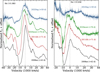 |
Fig. 20. SN 2022lxg He I NIR lines in velocity space and comparison with other Type IIb SNe: SN 2020acat (Medler et al. 2023), SN 2011dh (Ergon et al. 2015), and SN 2008ax (Roming et al. 2009). The spectra are binned to 5 Å for visual purposes and the original spectra are plotted with lighter colours in the background. The vertical grey line shows the central wavelength. Left: He I 1.0830 μm line. The spectra are normalised at ∼20 000 km s−1 red-wards of the central wavelength. Right: He I 2.0581 μm line. The spectra are normalised at ∼35 000 km s−1 red-wards of the central wavelength. |
4.1.3. Influence of the host environment
As previously noted, SN 2022lxg shows photometric and spectroscopic similarities with the P23 sample. Differences between these objects might be explained by variations in the amount and configuration of the CSM that lead to features appearing or disappearing at different times. Here we investigate whether this group of SNe also share similar environmental properties. In particular, we focus on the general lack of metal lines in the spectra (Sect. 3.3.2). Although it is possible that these may be suppressed by ongoing CSM interaction, one would have to tailor this effect across all objects in this group and across all epochs. The large projected host offset (∼4.6 kpc) of SN 2022lxg, and blue colours prompt us to consider whether low implied metallicity plays a role. This is further underscored by previous studies, albeit on Type IIP SNe, that noted a correlation between low-metallicity hosts (or explosion sites) and SN properties (e.g. Polshaw et al. 2016; Taddia et al. 2016; Gutiérrez et al. 2018).
In order to investigate a potential correlation with the metallicity of their hosts, we use archival photometry and the L − Z Tremonti et al. (2004) relation, in order to make some rough metallicity estimates. For SN 2022lxg, we use the archival PS g-band magnitude of the potential host (see Sect. 3.1), and after converting it to the B band (MB = −14.41 ± 0.10 mag, using the Jordi et al. 2006 colour transformations), we find 12 + log(O/H) = 7.90 ± 0.03, that is Z = (0.16 ± 0.01) Z⊙ (assuming 12 + log(O/H) = 8.69 for the Sun; Allende Prieto et al. 2001). The estimated metallicity is very low compared to the SDSS DR2 sample presented in Tremonti et al. (2004). We only find archival g-band photometry for three out of six SNe of the P23 sample, namely SN 2017cfo (that is spectroscopically the most similar to SN 2022lxg), SN 2017hxz (that is photometrically the most similar to SN 2022lxg) and SN 2018aql. We show the results in Fig. 21. We also include SN 2009Z, a Type IIb SN in a low surface brightness (LSB) galaxy (Zinn et al. 2012). Furthermore, we include the SESNe from the sample of Modjaz et al. (2011) in the comparison whose oxygen abundance was measured via strong-line diagnostics in the actual position of the SNe. Following Modjaz et al. (2011), we convert the oxygen abundance estimates derived with the empirical L − Z Tremonti et al. (2004) relation to the Pettini & Pagel (2004) strong-line diagnostic, using the empirical calibrations of Kewley & Ellison (2008). All the LSNe II have low metallicites compared to the bulk of the SDSS galaxies, with the faster ones (SN 2022lxg and SN 2017hxz) showing remarkably low metallicites. However, as demonstrated by Modjaz et al. (2011), the nuclear metallicity when derived from the SN host luminosity is not a good proxy for the local oxygen abundance of the environments of SNe: the local metallicities are often lower than the inferred central ones, something evident in Fig. 21. Hence, the true metallicities at the locations of those SNe might be even lower.
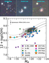 |
Fig. 21. Metallicity of host galaxies as a function of host absolute B magnitude. We have used the L − Z Tremonti et al. (2004) relation to estimate the metallicity of the (potential) host of SN 2022lxg, as well as some SNe from the P23 sample along with SN 2009Z, a Type IIb SN in a LSB galaxy. Contours show 50%, 75%, and 90% containment of the kernel density estimate of the SDSS DR2 sample presented in Tremonti et al. (2004). The metallicities where converted to the scale of PP04-O3N2 (solid line) including 1σ uncertainties (dashed lines), using the empirical calibrations of Kewley & Ellison (2008). The representative systematic error of 0.14 dex for the PP04-O3N2 scale is shown in the top left corner. We also include the SNe from the sample of Modjaz et al. (2011) in the comparison whose oxygen abundance was measured via strong-line diagnostics. The metallicity of the LSNe II hosts are consistently low compared to the sample, with the fastest events (SN 2022lxg and SN 2017hxz) having the lowest host metallicities. The top panels show a mosaic of gri coloured cutouts of the hosts of SN 2022lxg and two SNe from the P23 sample. A cyan cross denotes the position of the SN. From left to right we show: SN 2022lxg, SN 2017cfo, which is spectroscopically the most similar to SN 2022lxg, and SN 2017hxz, which is photometrically the most similar to SN 2022lxg. |
In spite of all the caveats in estimating metallicities from imaging, taken at face-value, it appears that the hosts of SNe such as SN 2022lxg are of low-metallicity, which would explain some of the properties of this group. Finally, the apparent similarities of 22lxg-like transients with SNe IIb is in line with the low-metallicity environment as studies of SN host environments that found SNe IIb to occur in distinctly different settings compared to other CC-SNe, typically in metal-poor regions with relatively low star formation rates (Galbany et al. 2018) or showing a significant excess in dwarf galaxy hosts (Arcavi et al. 2010). However, we note that other studies, based on comparable sample sizes (e.g. Pessi et al. 2023b) find that SNe IIb occur in higher metallicity environments compared to regular Type II SNe.
4.2. CSM configuration and a potential progenitor
We attempt here to make some rough estimates on the CSM mass and the mass-loss history of SN 2022lxg by making some basic assumptions; first, we assume homologous expansion and an ejecta velocity equal to 20 000 km s−1 (cf. Sect. 3.3). In order to cover a range of possible steady-state wind velocities of progenitor stars, we assume a value of 75 km s−1 typical value for a yellow supergiant (YSG) (Humphreys 2010; Humphreys et al. 2023), with ±25 km s−1 serving as our uncertainty estimates, leading to a CSM velocity range typical for RSG and YSG stars (Dessart & Jacobson-Galán 2023). The duration of the flash-ionisation features (∼8.24 days in our case, see Sect. 3.3.1) can indicate the extent of the CSM, assuming that the lines disappear when the SN ejecta sweep up the CSM where they originate. Based on our ejecta velocity estimate, that would be ∼1.42 × 1015 cm, which is where the peak of the blackbody radius lies (∼1.37 × 1015 cm). Assuming the aforementioned CSM velocities, that would suggest that the mass-loss started  years before the explosion. If we also assume a mass-loss rate (
 ), then we can infer the CSM mass. The models of Dessart & Jacobson-Galán (2023) that we compare to due to their resemblance to SN 2022lxg (see Sect. 4.1.1) have Ṁ = 1 × 10⁻³ M⊙ yr−1. If we use the relations between the mass-loss rate and duration of the flash-ionisation features (tIIn = 376.2 Ṁ) presented in Jacobson-Galán et al. (2024), we get a Ṁ ≃ 2.2 × 10⁻² M⊙ yr−1, while if we use our model fits (see Sect. 3.2.3), we can estimate the mass-loss rate at the inner radius of the CSM as
  , returning a Ṁ ≃ 4.3 × 10⁻³ M⊙ yr−1. We note however, that this calculation assumes spherical symmetry. These three different values for the mass-loss rate lead to a CSM mass (MCSM) of 0.006 M⊙, 0.132 M⊙, and 0.026 M⊙ respectively, with a mean value of
  . We stress however, that these estimates result from assumptions that may not hold over the timescales probed by our dataset. Nevertheless, they appear to be in line with values found in other studies.
However, apart from the interaction that gives rise to the flash-ionisation features, another phase of interaction appears to be taking place 35−40 days post-explosion (Sect. 4.1.1). As the optical depth of the ejecta drops and the photosphere recedes, the interaction with the CSM becomes more evident. One possibility might be that there is a change in the CSM density structure. Such a two-component CSM with different density structures has been previously invoked to explain the properties of SN 2018ivc, a Type IIb/IIL SN; that undergoes an extreme case of case C binary mass transfer resulting in a SN intermediate between SNe Ib/c and SNe IIP (Maeda et al. 2023b). The transitional properties of SN 2022lxg may well be a variant of such a scenario.
Another option for creating a two-component CSM would be a pre-explosion mass-loss episode, that is with an elevated mass-loss rate rather than a steady-state wind, that could be responsible for late signs of interaction. Making the same assumptions as before, but this time using the starting time of the late interaction signs (∼ + 40 d), we can probe where the inner layer of this potential eruption ejected CSM lies. We find that the material would lie at ∼6.9 × 1015 cm and assuming a conservative eruption velocity of 2000 ± 1000 km s−1 (observed velocities show even higher values, e.g. four SLSN-I show velocities spanning 3000−4400 km s−1; Gkini et al. 2025, or the 1843 eruption of η Carinae ∼3000 − 6000 km s−1; Smith 2008), the eruption should have occurred  years before the explosion. Observations of precursor emission to core-collapse SNe are a direct means of probing the enhanced mass-loss of the progenitor star during its final moments, especially if it is a violent eruption (Strotjohann et al. 2021). We requested forced photometry from ZTF, ATLAS, and ASAS-SN (Hart et al. 2023) for the pre-explosion epochs of SN 2022lxg in order to search for potential precursor emission. Forced photometry was combined into large ‘seasonal’ bins, defined by the longest unbroken runs of observations in a given observing season. The fluxes were combined using an inverse-variance weighting scheme, with sigma clipping applied to remove discrepant individual measurements in some surveys. New upper limits were recomputed based on the stacked fluxes and their uncertainties, with 5σ limits being used in practice. The results are presented in Fig. B.4. No significant pre-explosion emission is detected for SN 2022lxg. The forced photometry rules out long-lasting precursors with absolute magnitude M ≲ −11 mag that might have happened four years before the explosion. Data prior to that are not deep enough to rule out outbursts similar to those of other SNe. All the above considered, an eruption or sudden outburst seems less likely although cannot be entirely ruled out.
As previously noted, the rather low photospheric expansion velocity derived from the blackbody fits (∼7000 km s−1) is much lower than ejecta velocity derived from the spectroscopic lines and the light-curve model fits. Assuming a spherically symmetric CSM configuration and given the linear increase in the blackbody radius, the photosphere should lie nearly at the interacting region, that is, at the edge of the ejecta. This discrepancy between vph and vej, can potentially point to asphericity or line-of-sight (LOS) effects. Assuming a disc-like CSM around the progenitor if our LOS is along the low-density region and does not really intersect the dense CSM, we would expect broad lines (essentially unshocked ejecta) while the power can be provided by the off-LOS interaction (where the ejecta are decelerated, and vph can be much lower than the original unshocked ejecta velocity. Furthermore the imaging polarimetry at +17 d and +36 d (epochs at the start and the end of the cooling phase respectively) reveals that SN 2022lxg is intrinsically polarised to a p ∼ (0.5 − 1.0)% level (see Fig. 18). This points to the fact that there is some asphericity in the system. As the ejecta expand and the photosphere recedes, the temperature drops and the optical depth is decreasing so we start seeing more and more emission from the CSM component and less from the ejecta. The fact that Hα gradually starts getting centred after the crucial phase of 35 − 40 d (while it is blue-shifted until this point), means that even if the CSM is aspherical, it probably has a symmetric structure around the explosion. This could also point to an asymmetric (and potentially disc-like) CSM around the progenitor. Numerous examples of asymmetric CSM abound in the literature (e.g. Hoffman et al. 2008; Chornock et al. 2011; Smith et al. 2015; Mauerhan et al. 2015, 2017; Pursiainen et al. 2022; Reynolds et al. 2025b).
It has been suggested that strong late-time Hα profiles observed in some Type II SNe, arise due to late-time interaction with a disc-like CSM, when the photosphere recedes. Such profiles are sometimes red-shifted (e.g. PTF11iqb; Smith et al. 2015) or blue-shifted (e.g. SN 1998S; Leonard et al. 2000). Smith et al. (2015) suggest (their Fig. 10) that such disc-like CSM might arise from binaries with an azimuthally asymmetric density distribution around the disc/torus, with higher densities on the receding side. Such a disc/torus configuration was observed in the mass-transferring eclipsing binary RY Scuti (Smith et al. 2002b). If one of the stars explodes as a SN in such a system, a high-inclination observer would observe blue-shifted or red-shifted late-time Hα, depending on whether the LOS is towards the higher density or the lower density part of the CSM disc respectively. An observer at a low inclination (like the one we suggest that SN 2022lxg is viewed from) would see a narrower and more symmetric line profile. This is in agreement with the late-time centring of the Hα profile. Following (Smith et al. 2015), we present a schematic visualisation of a plausible physical evolution of SN 2022lxg in Fig. 22.
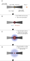 |
Fig. 22. Example of a possible configuration that gave rise to SN 2022lxg. We envisage a disc-like CSM (with a potentially azimuthally asymmetric density distribution) with the line-of-sight at a low inclination. (a) Before the explosion, we suggest that the CSM closest to the progenitor is denser and could have been formed by material transferred from a donor combined with stellar winds. (b) The fast-moving ejecta crash into the inner dense CSM giving rise to the observed flash-ionisation features and the luminous peak. Within ∼10−15 d this denser CSM is completely swept-up by the ejecta. (c) Between 10−35 d, the ejecta encounter the outer, hydrogen-rich, disc-like CSM and encompass it. Broad lines from the free-expanding, cooling ejecta emerge while the radius of the composite photoshpere plateaus. (d) After ∼35 d, the photosphere recedes, the optical depth of the ejecta drops, and the power comes from the interaction. Narrower Hα emerges and dominates the spectrum. |
In summary, taking all the clues into account, we find that a plausible scenario for explaining the salient properties of SN 2022lxg and related objects could be to use our findings from Sect. 4.1.3 as our starting point. Previous studies of massive binary evolution have shown an inverse correlation between the size of massive stars and metallicity (e.g. Brott et al. 2011; Georgy et al. 2013; Schootemeijer et al. 2019). Thus if we consider mass transfer in a close binary, required to create a CSM with the properties as described above, then it is likely that mass transfer via Roche lobe overflow occurs only late in the evolution (case C) as the progenitor is too compact during earlier evolutionary stages. The resulting CSM would then naturally have a preferred axial symmetry. With this framework, the rapid rise to peak brightness, the colour evolution, and the spectral behaviour can be qualitatively explained. Furthermore, the apparent rarity of such objects also follows, although larger sample sizes are warranted.
5. Conclusions
We have presented the analysis of the optical and NIR properties of SN 2022lxg, a peculiar, bright (Mg = −19.41 mag at peak), and fast evolving SN at ∼96.6 Mpc. Based on our analysis we find the following:
-
The most probable host galaxy is a faint (Mr = −15.2) and diffuse source (WISEA J191523.71+481938.5) 4.58 kpc NW from the location of the SN.
-
The SN is luminous and peaks at Mg = −19.41 mag. The rise and the decline are relatively fast, 7.6 days from explosion (for which we put very tight constraints) to peak, and a decline of 3.48 ± 0.26 mag (50 d)−1 (both in the g band). The SN slows down around the peak epochs, where we might see a hint of the shock breakout cooling in the light-curves, blended with the power from the interaction (responsible for the luminous peak).
-
The spectral evolution can be divided into three phases:
-
Until ten days post explosion, the SN shows very blue continua (T > 15 000 K) with flash-ionisation features of hydrogen and He II until ∼ + 8 d.
-
Between roughly +10 to +35 d, the SN cools and broad (∼2 × 10⁴ km s−1) lines appear, identified as hydrogen, helium, a strong iron complex around 5300 Å and the Ca II NIR triplet. At this phase, there are striking similarities with early spectra of SNe IIb.
-
After ∼ + 35 d, a previously blue-shifted Hα gets centred to the rest wavelength, becomes narrower, and its pseudo-equivalent width rises sharply, dominating the spectra until +80 d, when our spectroscopic follow-up stops as the SN is already too faint (mg ∼ 20 mag).
-
-
4.
Using various standard methods and light-curve model fits, we find that SN 2022lxg must have a low amount of 56Ni (≲0.013 M⊙). Several signs point to interaction between the ejecta and circumstellar material (CSM) such as the luminous peak (despite the very low 56Ni mass), the fast rise, the late (≳ + 35 d) spectral transitioning, and narrow (∼100 km s−1) He I 1.0830 μm P-Cygni lines, which reveal unshocked helium CSM and suggest partial stripping of the progenitor.
-
5.
A discrepancy between the photospheric and the ejecta velocity (7000 compared to 20 000 km s−1) might potentially point to line-of-sight effects and asphericity. This is further confirmed by two epochs of imaging polarimetry in the V and R filters that show intrinsic polarisation of p ∼ (0.5 − 1.0)%.
-
6.
SN 2022lxg shares many similar properties with a sample of LSNe II, such as higher luminosity, fast decline, blue colours, lack of persistent narrow lines, broad Hα emission, He I 5876 Å emission, and weak or non-existent Hα absorption and metal lines. There is tentative evidence that the properties of these SNe might be correlated with the low-metallicity of their host galaxies, however the numbers are still too low to draw statistically robust conclusions.
-
7.
We can reconcile most of the observed properties of SN 2022lxg by invoking late mass transfer in a close binary system that gives rise to a disc-like CSM oriented such that our line of sight does not directly traverse it. As the optical depth of the ejecta drops and the photosphere recedes, the interaction with the CSM becomes dominant, which leads to a spectroscopic change from a SN IIb to spectra that are more akin to an interacting SN II.
Data availability
Table A.1 is available at the CDS via https://cdsarc.cds.unistra.fr/viz-bin/cat/J/A+A/700/A138
Foscgui is a graphic user interface aimed at extracting SN spectroscopy and photometry obtained with FOSC-like instruments. It was developed by E. Cappellaro. A package description can be found at https://sngroup.oapd.inaf.it/foscgui.html
Acknowledgments
We thank the anonymous referee for the helpful comments that improved the manuscript. We thank T. Nagao for many interesting discussions and providing the imaging polarimetry data presented in Sect. 3.4. R.K. also acknowledges discussions with L. Dessart. P.C., R.K., and T.L.K. acknowledge support via the Research Council of Finland (grant 340613). C.P.G. acknowledges financial support from the Secretary of Universities and Research (Government of Catalonia) and by the Horizon 2020 Research and Innovation Programme of the European Union under the Marie Skłodowska-Curie and the Beatriu de Pinós 2021 BP 00168 programme, from the Spanish Ministerio de Ciencia e Innovación (MCIN) and the Agencia Estatal de Investigación (AEI) 10.13039/501100011033 under the PID2020-115253GA-I00 HOSTFLOWS project, and the program Unidad de Excelencia María de Maeztu CEX2020-001058-M. M.P. acknowledges support from a UK Research and Innovation Fellowship (MR/T020784/1). T.L.K. acknowledges support from the Turku University Foundation (grant no. 081810). S.S. is partially supported by LBNL Subcontract 7707915. K.M. acknowledges support from the Japan Society for the Promotion of Science (JSPS) KAKENHI grant JP24KK0070 and 24H01810. The work is partly supported by the JSPS Open Partnership Bilateral Joint Research Projects between Japan and Finland (JPJSBP120229923). T.K. acknowledges support from the Research Council of Finland project 360274. Y.-Z.C. is supported by the National Natural Science Foundation of China (NSFC, Grant No. 12303054), the National Key Research and Development Program of China (Grant No. 2024YFA1611603), the Yunnan Fundamental Research Projects (Grant Nos. 202401AU070063, 202501AS070078), and the International Centre of Supernovae, Yunnan Key Laboratory (No. 202302AN360001). E.K. acknowledges financial support from the Emil Aaltonen foundation. H.K. was funded by the Research Council of Finland projects 324504, 328898, and 353019. S.M. and T.M.R. acknowledge support from the Research Council of Finland project 350458. A.R. acknowledges financial support from the GRAWITA Large Program Grant (PI P. D’Avanzo) and from the PRIN-INAF 2022 Shedding light on the nature of gap transients: from the observations to the models. T.M.R. is part of the Cosmic Dawn Center (DAWN), which is funded by the Danish National Research Foundation under grant DNRF140. M.D.S. is funded by the Independent Research Fund Denmark (IRFD, grant number 10.46540/2032-00022B) and by an Aarhus University Research Foundation Nova project (AUFF-E-2023-9-28). Based on observations obtained with the Samuel Oschin Telescope 48-inch and the 60-inch Telescope at the Palomar Observatory as part of the Zwicky Transient Facility project. ZTF is supported by the National Science Foundation under Grants No. AST-1440341 and AST-2034437 and a collaboration including Caltech, IPAC, the Weizmann Institute of Science, the Oskar Klein Center at Stockholm University, the University of Maryland, Deutsches Elektronen-Synchrotron and Humboldt University, the TANGO Consortium of Taiwan, the University of Wisconsin at Milwaukee, Trinity College Dublin, Lawrence Livermore National Laboratories, IN2P3, University of Warwick, Ruhr University Bochum, Northwestern University and former partners the University of Washington, Los Alamos National Laboratories, and Lawrence Berkeley National Laboratories. Operations are conducted by COO, IPAC, and UW. SED Machine is based upon work supported by the National Science Foundation under Grant No. 1106171. The ZTF forced-photometry service was funded under the Heising-Simons Foundation grant #12540303 (PI: Graham). The Gordon and Betty Moore Foundation, through both the Data-Driven Investigator Program and a dedicated grant, provided critical funding for SkyPortal. Based on observations made with the Nordic Optical Telescope, owned in collaboration by the University of Turku and Aarhus University, and operated jointly by Aarhus University, the University of Turku and the University of Oslo, representing Denmark, Finland, and Norway, the University of Iceland and Stockholm University at the Observatorio del Roque de los Muchachos, La Palma, Spain, of the Instituto de Astrofisica de Canarias. The data presented here were obtained with ALFOSC, which is provided by the Instituto de Astrofisica de Andalucia (IAA) under a joint agreement with the University of Copenhagen and NOT. Observations from the Nordic Optical Telescope were obtained through the NUTS2 collaboration which is supported in part by the Instrument Centre for Danish Astrophysics (IDA), and the Finnish Centre for Astronomy with ESO (FINCA) via Academy of Finland grant nr 306531, through the proposal P65-005 (PI: T. Nagao), and through the fast-track proposal P66-415 (PI: P. Charalampopoulos).
References
- Allende Prieto, C., Lambert, D. L., & Asplund, M. 2001, ApJ, 556, L63 [Google Scholar]
- Anderson, J. P., González-Gaitán, S., Hamuy, M., et al. 2014a, ApJ, 786, 67 [Google Scholar]
- Anderson, J. P., Dessart, L., Gutierrez, C. P., et al. 2014b, MNRAS, 441, 671 [NASA ADS] [CrossRef] [Google Scholar]
- Andrews, J. E., & Smith, N. 2018, MNRAS, 477, 74 [Google Scholar]
- Andrews, J. E., Shrestha, M., Bostroem, K. A., et al. 2025, ApJ, 980, 37 [Google Scholar]
- Arcavi, I., Gal-Yam, A., Kasliwal, M. M., et al. 2010, ApJ, 721, 777 [NASA ADS] [CrossRef] [Google Scholar]
- Arcavi, I., Gal-Yam, A., Yaron, O., et al. 2011, ApJ, 742, L18 [Google Scholar]
- Arnett, W. D. 1982, ApJ, 253, 785 [Google Scholar]
- Ashall, C. 2022, Transient Name Server Classification Report, No. 2022-1602, 1 [Google Scholar]
- Barbary, K., Dawson, K. S., Tokita, K., et al. 2009, ApJ, 690, 1358 [NASA ADS] [CrossRef] [Google Scholar]
- Barnsley, R., Smith, R., & Steele, I. 2012, Astron. Nachr., 333, 101 [NASA ADS] [CrossRef] [Google Scholar]
- Bellm, E. C., Kulkarni, S. R., Graham, M. J., et al. 2019, PASP, 131, 018002 [Google Scholar]
- Benetti, S., Chugai, N. N., Utrobin, V. P., et al. 2016, MNRAS, 456, 3296 [NASA ADS] [CrossRef] [Google Scholar]
- Bersten, M. C., Benvenuto, O. G., Nomoto, K., et al. 2012, ApJ, 757, 31 [Google Scholar]
- Blagorodnova, N., Neill, J. D., Walters, R., et al. 2018, PASP, 130, 035003 [Google Scholar]
- Blondin, S., & Tonry, J. L. 2007, ApJ, 666, 1024 [NASA ADS] [CrossRef] [Google Scholar]
- Bostroem, K. A., Valenti, S., Sand, D. J., et al. 2020, ApJ, 895, 31 [NASA ADS] [CrossRef] [Google Scholar]
- Bradley, L., Sipőcz, B., Robitaille, T., et al. 2024, https://doi.org/10.5281/zenodo.596036 [Google Scholar]
- Branch, D., Falk, S. W., Uomoto, A. K., et al. 1981, ApJ, 244, 780 [Google Scholar]
- Brott, I., de Mink, S. E., Cantiello, M., et al. 2011, A&A, 530, A115 [NASA ADS] [CrossRef] [EDP Sciences] [Google Scholar]
- Bruch, R. J., Gal-Yam, A., Schulze, S., et al. 2021, ApJ, 912, 46 [NASA ADS] [CrossRef] [Google Scholar]
- Bruch, R. J., Gal-Yam, A., Yaron, O., et al. 2023, ApJ, 952, 119 [NASA ADS] [CrossRef] [Google Scholar]
- Bufano, F., Pignata, G., Bersten, M., et al. 2014, MNRAS, 439, 1807 [Google Scholar]
- Cappellaro, E., Mazzali, P. A., Benetti, S., et al. 1997, A&A, 328, 203 [NASA ADS] [Google Scholar]
- Cardelli, J. A., Clayton, G. C., & Mathis, J. S. 1989, ApJ, 345, 245 [Google Scholar]
- Chatzopoulos, E., Craig Wheeler, J., & Vinko, J. 2012, ApJ, 746, 121 [Google Scholar]
- Chatzopoulos, E., Wheeler, J. C., Vinko, J., Horvath, Z. L., & Nagy, A. 2013, ApJ, 773, 76 [NASA ADS] [CrossRef] [Google Scholar]
- Chevalier, R. A., & Irwin, C. M. 2011, ApJ, 729, L6 [Google Scholar]
- Chornock, R., Filippenko, A. V., Li, W., et al. 2011, ApJ, 739, 41 [NASA ADS] [CrossRef] [Google Scholar]
- Chugai, N. N. 2001, MNRAS, 326, 1448 [NASA ADS] [CrossRef] [Google Scholar]
- Chugai, N. N. 2009, MNRAS, 400, 866 [CrossRef] [Google Scholar]
- Claeys, J. S., De Mink, S. E., Pols, O. R., Eldridge, J. J., & Baes, M. 2011, A&A, 528, A131 [NASA ADS] [CrossRef] [EDP Sciences] [Google Scholar]
- Davis, S., Hsiao, E. Y., Ashall, C., et al. 2019, ApJ, 887, 4 [NASA ADS] [CrossRef] [Google Scholar]
- de Jaeger, T., Anderson, J. P., Galbany, L., et al. 2018, MNRAS, 476, 4592 [NASA ADS] [CrossRef] [Google Scholar]
- de Vaucouleurs, G., de Vaucouleurs, A., Buta, R., Ables, H. D., & Hewitt, A. V. 1981, PASP, 93, 36 [NASA ADS] [CrossRef] [Google Scholar]
- Dekany, R., Smith, R. M., Riddle, R., et al. 2020, PASP, 132, 038001 [NASA ADS] [CrossRef] [Google Scholar]
- D’Elia, V., Pian, E., Melandri, A., et al. 2015, A&A, 577, A116 [NASA ADS] [CrossRef] [EDP Sciences] [Google Scholar]
- Dessart, L., & Hillier, D. J. 2022, A&A, 660, L9 [NASA ADS] [CrossRef] [EDP Sciences] [Google Scholar]
- Dessart, L., & Jacobson-Galán, W. V. 2023, A&A, 677, A105 [NASA ADS] [CrossRef] [EDP Sciences] [Google Scholar]
- Dessart, L., Hillier, D. J., & Audit, E. 2017, A&A, 605, A83 [NASA ADS] [CrossRef] [EDP Sciences] [Google Scholar]
- Ercolino, A., Jin, H., Langer, N., & Dessart, L. 2024, A&A, 685, A58 [NASA ADS] [CrossRef] [EDP Sciences] [Google Scholar]
- Ergon, M., Jerkstrand, A., Sollerman, J., et al. 2015, A&A, 580, A142 [NASA ADS] [CrossRef] [EDP Sciences] [Google Scholar]
- Faran, T., Poznanski, D., Filippenko, A. V., et al. 2014, MNRAS, 445, 554 [NASA ADS] [CrossRef] [Google Scholar]
- Fassia, A., Meikle, W. P., Vacca, W. D., et al. 2000, MNRAS, 318, 1093 [NASA ADS] [CrossRef] [Google Scholar]
- Filippenko, A. V., Matheson, T., & Ho, L. C. 1993, ApJ, 415, L103 [NASA ADS] [CrossRef] [Google Scholar]
- Foley, R. J., Smith, N., Ganeshalingam, M., et al. 2007, ApJ, 657, L105 [NASA ADS] [CrossRef] [Google Scholar]
- Fransson, C., Challis, P. M., Chevalier, R. A., et al. 2005, ApJ, 622, 991 [NASA ADS] [CrossRef] [Google Scholar]
- Fremling, C., Sollerman, J., Taddia, F., et al. 2016, A&A, 593, A68 [NASA ADS] [CrossRef] [EDP Sciences] [Google Scholar]
- Galbany, L., Anderson, J. P., Sánchez, S. F., et al. 2018, ApJ, 855, 107 [Google Scholar]
- Gall, E. E., Polshaw, J., Kotak, R., et al. 2015, A&A, 582, A3 [NASA ADS] [CrossRef] [EDP Sciences] [Google Scholar]
- Gal-Yam, A., Arcavi, I., Ofek, E. O., et al. 2014, Nature, 509, 471 [CrossRef] [Google Scholar]
- Georgy, C., Ekström, S., Eggenberger, P., et al. 2013, A&A, 558, A103 [NASA ADS] [CrossRef] [EDP Sciences] [Google Scholar]
- Gezari, S., Halpern, J. P., Grupe, D., et al. 2009, ApJ, 690, 1313 [NASA ADS] [CrossRef] [Google Scholar]
- Gkini, A., Fransson, C., Lunnan, R., et al. 2025, A&A, 694, A292 [NASA ADS] [CrossRef] [EDP Sciences] [Google Scholar]
- González-Gaitán, S., Tominaga, N., Molina, J., et al. 2015, MNRAS, 451, 2212 [CrossRef] [Google Scholar]
- Graham, M. J., Kulkarni, S. R., Bellm, E. C., et al. 2019, PASP, 131, 078001 [Google Scholar]
- Guillochon, J., Nicholl, M., Villar, V. A., et al. 2018, ApJS, 236, 6 [NASA ADS] [CrossRef] [Google Scholar]
- Gutiérrez, C. P., Anderson, J. P., Hamuy, M., et al. 2014, ApJ, 786, L15 [CrossRef] [Google Scholar]
- Gutiérrez, C. P., Anderson, J. P., Hamuy, M., et al. 2017, ApJ, 850, 89 [CrossRef] [Google Scholar]
- Gutiérrez, C. P., Anderson, J. P., Sullivan, M., et al. 2018, MNRAS, 479, 3232 [CrossRef] [Google Scholar]
- Gutiérrez, C. P., Pastorello, A., Jerkstrand, A., et al. 2020, MNRAS, 499, 974 [CrossRef] [Google Scholar]
- Güver, T., & Özel, F. 2009, MNRAS, 400, 2050 [Google Scholar]
- Hamuy, M. 2003, ApJ, 582, 905 [NASA ADS] [CrossRef] [Google Scholar]
- Hart, K., Shappee, B. J., Hey, D., et al. 2023, ArXiv e-prints [arXiv:2304.03791] [Google Scholar]
- Harutyunyan, A. H., Pfahler, P., Pastorello, A., et al. 2008, A&A, 488, 383 [NASA ADS] [CrossRef] [EDP Sciences] [Google Scholar]
- Heiles, C. 2000, AJ, 119, 923 [Google Scholar]
- Ho, A. Y. Q., Perley, D. A., Gal-Yam, A., et al. 2023, ApJ, 949, 120 [NASA ADS] [CrossRef] [Google Scholar]
- Hoffman, J. L., Leonard, D. C., Chornock, R., et al. 2008, ApJ, 688, 1186 [NASA ADS] [CrossRef] [Google Scholar]
- Hoflich, P. 1991, A&A, 246, 481 [NASA ADS] [Google Scholar]
- Huber, M., Chambers, K. C., Flewelling, H., et al. 2015, ATel, 7153, 1 [NASA ADS] [Google Scholar]
- Humphreys, R. 2010, ASP Conf. Ser., 425, 247 [Google Scholar]
- Humphreys, R. M., Jones, T. J., & Martin, J. C. 2023, AJ, 166, 50 [NASA ADS] [CrossRef] [Google Scholar]
- Jacobson-Galán, W. V., Dessart, L., Davis, K. W., et al. 2024, ApJ, 970, 189 [CrossRef] [Google Scholar]
- Jordi, K., Grebel, E. K., & Ammon, K. 2006, A&A, 460, 339 [NASA ADS] [CrossRef] [EDP Sciences] [Google Scholar]
- Kaiser, N., Aussel, H., Burke, B. E., et al. 2002, Proc. SPIE, 4836, 154 [NASA ADS] [CrossRef] [Google Scholar]
- Kewley, L. J., & Ellison, S. L. 2008, ApJ, 681, 1183 [Google Scholar]
- Khazov, D., Yaron, O., Gal-Yam, A., et al. 2016, ApJ, 818, 3 [CrossRef] [Google Scholar]
- Kim, Y. L., Rigault, M., Neill, J. D., et al. 2022, PASP, 134, 024505 [NASA ADS] [CrossRef] [Google Scholar]
- Kotak, R., Meikle, W. P., Adamson, A., & Leggett, S. K. 2004, MNRAS, 354, L13 [CrossRef] [Google Scholar]
- Kulkarni, S. R., Frail, D. A., Wieringa, M. H., et al. 1998, Nature, 395, 663 [NASA ADS] [CrossRef] [Google Scholar]
- Langer, N. 1998, A&A, 329, 551 [NASA ADS] [Google Scholar]
- Langer, N. 2012, ARA&A, 50, 107 [CrossRef] [Google Scholar]
- Leloudas, G., Maund, J. R., Gal-Yam, A., et al. 2017, ApJ, 837, L14 [NASA ADS] [CrossRef] [Google Scholar]
- Leonard, D. C., Filippenko, A. V., Barth, A. J., & Matheson, T. 2000, ApJ, 536, 239 [Google Scholar]
- Maeda, K., Chandra, P., Moriya, T. J., et al. 2023a, ApJ, 942, 17 [NASA ADS] [CrossRef] [Google Scholar]
- Maeda, K., Michiyama, T., Chandra, P., et al. 2023b, ApJ, 945, L3 [NASA ADS] [CrossRef] [Google Scholar]
- Mandigo-Stoba, M. S., Fremling, C., & Kasliwal, M. M. 2022, J. Open Source Softw., 7, 3612 [NASA ADS] [CrossRef] [Google Scholar]
- Masci, F. J., Laher, R. R., Rusholme, B., et al. 2019, PASP, 131, 018003 [Google Scholar]
- Mauerhan, J., Smith, N., Van Dyk, S. D., et al. 2015, MNRAS, 450, 2551 [Google Scholar]
- Mauerhan, J. C., Van Dyk, S. D., Johansson, J., et al. 2017, ApJ, 834, 118 [Google Scholar]
- Medler, K., Mazzali, P. A., Teffs, J., et al. 2022, MNRAS, 513, 5540 [NASA ADS] [CrossRef] [Google Scholar]
- Medler, K., Mazzali, P. A., Ashall, C., et al. 2023, MNRAS, 518, L40 [Google Scholar]
- Meynet, G., Maeder, A., Schaller, G., Schaerer, D., & Charbonnel, C. 1994, A&AS, 103, 97 [Google Scholar]
- Miller, A. A., Chornock, R., Perley, D. A., et al. 2009, ApJ, 690, 1303 [NASA ADS] [CrossRef] [Google Scholar]
- Modjaz, M., Kewley, L., Bloom, J. S., et al. 2011, ApJ, 731, L4 [NASA ADS] [CrossRef] [Google Scholar]
- Morales-Garoffolo, A., Elias-Rosa, N., Benetti, S., et al. 2014, MNRAS, 445, 1647 [Google Scholar]
- Morales-Garoffolo, A., Elias-Rosa, N., Bersten, M., et al. 2015, MNRAS, 454, 95 [CrossRef] [Google Scholar]
- Moriya, T. J., & Tominaga, N. 2012, ApJ, 747, 118 [Google Scholar]
- Nadyozhin, D. K. 1994, ApJS, 92, 527 [Google Scholar]
- Nagy, A. P. 2018, ApJ, 862, 143 [Google Scholar]
- Nicholl, M. 2018, Res. Notes AAS, 2, 230 [NASA ADS] [CrossRef] [Google Scholar]
- Nomoto, K., Suzuki, T., Shigeyama, T., et al. 1993, Nature, 364, 507 [Google Scholar]
- Nomoto, K., Iwamoto, K., & Suzuki, T. 1995, Phys. Rep., 256, 173 [CrossRef] [Google Scholar]
- Oke, J. B., & Gunn, J. E. 1983, ApJ, 266, 713 [NASA ADS] [CrossRef] [Google Scholar]
- Oke, J. B., Cohen, J. G., Carr, M., et al. 1995, PASP, 107, 375 [Google Scholar]
- Ouchi, R., Maeda, K., Anderson, J. P., & Sawada, R. 2021, ApJ, 922, 141 [CrossRef] [Google Scholar]
- Pastorello, A., Prieto, J. L., Elias-Rosa, N., et al. 2015, MNRAS, 453, 3649 [Google Scholar]
- Patat, F., Barbon, R., Cappellaro, E., et al. 1994, A&A, 282, 731 [Google Scholar]
- Patat, F., Cappellaro, E., Danziger, J., et al. 2001, ApJ, 555, 900 [Google Scholar]
- Perley, D. A., Mazzali, P. A., Yan, L., et al. 2019, MNRAS, 484, 1031 [Google Scholar]
- Perley, D. A., Sollerman, J., Schulze, S., et al. 2022, ApJ, 927, 180 [NASA ADS] [CrossRef] [Google Scholar]
- Pessi, P. J., Anderson, J. P., Folatelli, G., et al. 2023a, MNRAS, 523, 5315 [NASA ADS] [CrossRef] [Google Scholar]
- Pessi, T., Prieto, J. L., Anderson, J. P., et al. 2023b, A&A, 677, A28 [NASA ADS] [CrossRef] [EDP Sciences] [Google Scholar]
- Pettini, M., & Pagel, B. E. 2004, MNRAS, 348, L59 [NASA ADS] [CrossRef] [Google Scholar]
- Piascik, A. S., Steele, I. A., Bates, S. D., et al. 2014, Proc. SPIE, 9147, 91478H [Google Scholar]
- Planck Collaboration VI. 2020, A&A, 641, A6 [NASA ADS] [CrossRef] [EDP Sciences] [Google Scholar]
- Plaszczynski, S., Montier, L., Levrier, F., & Tristram, M. 2014, MNRAS, 439, 4048 [NASA ADS] [CrossRef] [Google Scholar]
- Podsiadlowski, P. 1992, PASP, 104, 717 [CrossRef] [Google Scholar]
- Polshaw, J., Kotak, R., Dessart, L., et al. 2016, A&A, 588, A1 [NASA ADS] [CrossRef] [EDP Sciences] [Google Scholar]
- Prochaska, J., Hennawi, J., Westfall, K., et al. 2020, J. Open Source Softw., 5, 2308 [NASA ADS] [CrossRef] [Google Scholar]
- Pursiainen, M., Leloudas, G., Paraskeva, E., et al. 2022, A&A, 666, A30 [NASA ADS] [CrossRef] [EDP Sciences] [Google Scholar]
- Pursiainen, M., Leloudas, G., Cikota, A., et al. 2023, A&A, 674, A81 [NASA ADS] [CrossRef] [EDP Sciences] [Google Scholar]
- Reguitti, A., Dastidar, R., Pignata, G., et al. 2024, A&A, 692, A26 [NASA ADS] [CrossRef] [EDP Sciences] [Google Scholar]
- Reynolds, T. M., Fraser, M., Mattila, S., et al. 2020, MNRAS, 493, 1761 [NASA ADS] [CrossRef] [Google Scholar]
- Reynolds, T. M., Nagao, T., Gottumukkala, R., et al. 2025a, A&A, submitted [arXiv:2501.13619] [Google Scholar]
- Reynolds, T. M., Nagao, T., Maeda, K., et al. 2025b, A&A, submitted [arXiv:2501.13621] [Google Scholar]
- Richmond, M. W., Treffers, R. R., Filippenko, A. V., et al. 1994, AJ, 107, 1022 [Google Scholar]
- Rigault, M., Neill, J. D., Blagorodnova, N., et al. 2019, A&A, 627, A115 [NASA ADS] [CrossRef] [EDP Sciences] [Google Scholar]
- Rodrigo, C., & Solano, E. 2020, Contributions to the XIV.0 Scientific Meeting (virtual) of the Spanish Astronomical Society, 182 [Google Scholar]
- Rodrigo, C., Solano, E., & Bayo, A. 2012, SVO Filter Profile Service Version 1.0, International Virtual Observatory Alliance [Google Scholar]
- Rodrigo, C., Cruz, P., Aguilar, J. F., et al. 2024, A&A, 689, A93 [NASA ADS] [CrossRef] [EDP Sciences] [Google Scholar]
- Rodríguez, Ó., Maoz, D., & Nakar, E. 2023, ApJ, 955, 71 [CrossRef] [Google Scholar]
- Roming, P. W., Pritchard, T. A., Brown, P. J., et al. 2009, ApJ, 704, L118 [Google Scholar]
- Sahu, D. K., Tanaka, M., Anupama, G. C., Gurugubelli, U. K., & Nomoto, K. 2009, ApJ, 697, 676 [Google Scholar]
- Schlafly, E. F., & Finkbeiner, D. P. 2011, ApJ, 737, 103 [Google Scholar]
- Schlegel, E. M. 1990, MNRAS, 244, 269 [NASA ADS] [Google Scholar]
- Schootemeijer, A., Langer, N., Grin, N. J., & Wang, C. 2019, A&A, 625, A132 [NASA ADS] [CrossRef] [EDP Sciences] [Google Scholar]
- Seeger, M. 2004, Int. J. Neural Syst., 14, 69 [Google Scholar]
- Serkowski, K., Mathewson, D. L., & Ford, V. L. 1975, ApJ, 196, 261 [NASA ADS] [CrossRef] [Google Scholar]
- Shappee, B., Prieto, J., Stanek, K. Z., et al. 2014, Am. Astron. Soc., 223, 236.03 [NASA ADS] [Google Scholar]
- Shingles, L., Smith, K. W., Young, D. R., et al. 2021, TNSAN, 7, 1 [NASA ADS] [Google Scholar]
- Shivvers, I., Groh, J. H., Mauerhan, J. C., et al. 2015, ApJ, 806, 213 [NASA ADS] [CrossRef] [Google Scholar]
- Simmons, J. F. L., & Stewart, B. G. 1985, A&A, 142, 100 [NASA ADS] [Google Scholar]
- Smith, N. 2008, Nature, 455, 201 [Google Scholar]
- Smith, N., Gehrz, R. D., Stahl, O., Balick, B., & Kaufer, A. 2002a, ApJ, 578, 464 [NASA ADS] [CrossRef] [Google Scholar]
- Smith, J. A., Tucker, D. L., Kent, S., et al. 2002b, AJ, 123, 2121 [NASA ADS] [CrossRef] [Google Scholar]
- Smith, N., Silverman, J. M., Chornock, R., et al. 2009, ApJ, 695, 1334 [Google Scholar]
- Smith, N., Mauerhan, J. C., Cenko, S. B., et al. 2015, MNRAS, 449, 1876 [Google Scholar]
- Smith, K. W., Smartt, S. J., Young, D. R., et al. 2020, PASP, 132, 1 [Google Scholar]
- Speagle, J. S. 2020, MNRAS, 493, 3132 [Google Scholar]
- Stanek, K. Z. 2022, Transient Name Server Discovery Report, No. 2022-1548, 1 [Google Scholar]
- Steele, I. A. 2004, Astron. Nachr., 325, 519 [NASA ADS] [CrossRef] [Google Scholar]
- Stritzinger, M., Taddia, F., Fransson, C., et al. 2012, ApJ, 756, 173 [NASA ADS] [CrossRef] [Google Scholar]
- Strotjohann, N. L., Ofek, E. O., Gal-Yam, A., et al. 2021, ApJ, 907, 99 [NASA ADS] [CrossRef] [Google Scholar]
- Taddia, F., Moquist, P., Sollerman, J., et al. 2016, A&A, 587, L7 [NASA ADS] [CrossRef] [EDP Sciences] [Google Scholar]
- Tinyanont, S., Foley, R. J., Taggart, K., et al. 2024, PASP, 136, 014201 [Google Scholar]
- Tonry, J. L., Denneau, L., Heinze, A. N., et al. 2018, PASP, 130, 064505 [Google Scholar]
- Tremonti, C. A., Heckman, T. M., Kauffmann, G., et al. 2004, ApJ, 613, 898 [Google Scholar]
- Trundle, C., Kotak, R., Vink, J. S., & Meikle, W. P. 2008, A&A, 483, L47 [NASA ADS] [CrossRef] [EDP Sciences] [Google Scholar]
- Valenti, S., Howell, D. A., Stritzinger, M. D., et al. 2016, MNRAS, 459, 3939 [NASA ADS] [CrossRef] [Google Scholar]
- Wang, L., Wheeler, J. C., & Höflich, P. 1997, ApJ, 476, L27 [NASA ADS] [CrossRef] [Google Scholar]
- Wheeler, J. C., Barker, E., Benjamin, R., et al. 1993, ApJ, 417, L71 [NASA ADS] [CrossRef] [Google Scholar]
- Woosley, S. E., Hartmann, D., & Pinto, P. A. 1989, ApJ, 346, 395 [NASA ADS] [CrossRef] [Google Scholar]
- Woosley, S. E., Eastman, R. G., Weaver, T. A., & Pinto, P. A. 1994, ApJ, 429, 300 [NASA ADS] [CrossRef] [Google Scholar]
- Woosley, S. E., Eastman, R. G., & Schmidt, B. P. 1999, ApJ, 516, 788 [NASA ADS] [CrossRef] [Google Scholar]
- Woosley, S. E., Heger, A., & Weaver, T. A. 2002, Rev. Mod. Phys., 74, 1015 [NASA ADS] [CrossRef] [Google Scholar]
- Yaron, O., & Gal-Yam, A. 2012, PASP, 124, 668 [Google Scholar]
- Yaron, O., Perley, D. A., Gal-Yam, A., et al. 2017, Nat. Phys., 13, 510 [NASA ADS] [CrossRef] [Google Scholar]
- Yoon, S.-C., Dessart, L., & Clocchiatti, A. 2017, ApJ, 840, 10 [NASA ADS] [CrossRef] [Google Scholar]
- Zinn, P. C., Stritzinger, M., Braithwaite, J., et al. 2012, A&A, 538, A30 [NASA ADS] [CrossRef] [EDP Sciences] [Google Scholar]
Appendix A: Tables
Spectroscopic observations of SN 2022lxg
56Ni mass estimates for SN 2022lxg.
Imaging polarimetry observations of SN 2022lxg with ALFOSC.
Appendix B: Supplementary figures
 |
Fig. B.1. Posterior probability density functions for the free parameters of the model light-curves in Fig. 9. |
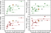 |
Fig. B.2. Comparison of the timescale of the He II flash-ionisation feature versus the peak absolute magnitude (left panels) and the rise time (right panels), for various SNe (adapted from Bruch et al. 2023). Top panels are in the g band while bottom panels in the r band. SN 2022lxg is shown as a star, where the filled or empty markers denote two potential timescales (8.24 and 11.63 days respectively; see Sect. 3.3.1. The filled circles are a sample of SNe showing flash-ionisation features taken from Bruch et al. (2023). |
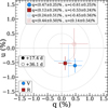 |
Fig. B.3. Intensity-normalised Stokes q and u parameters, from ALFOSC imaging polarimetry, in the V (blue circles) and R (red squares) bands, at phases +17.4 d (filled markers) and +36.1 d (open markers). The values are corrected for the ISP contribution. The dashed circles mark the 0.5%, 1.0% and 1.5% polarisation values (p). The first epoch (with a good S/N ratio ∼ 300) shows that SN 2022lxg is intrinsically polarised to a p ∼ (0.5 − 1.0)% level. |
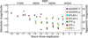 |
Fig. B.4. Pre-explosion forced photometry at the location of SN 2022lxg from ZTF, ATLAS and ASAS-SN. Individual epochs have been binned per season. Non-detections are shown as downward-facing triangles. The peak time is shown as a dashed vertical line. No significant pre-explosion emission is detected for SN 2022lxg. The forced photometry rules out long-lasting precursors with absolute magnitude M ≲ −11 mag that might have happened within four years prior to explosion, but before that, they are not deep enough to rule out outbursts similar to those of other SNe. |
All Tables
All Figures
|
Fig. 1. r band image showing SN 2022lxg (α = 19h15m23.630s, δ = +48° 19′27.70″, J2000), taken with NOT+ALFOSC on 25 July 2022 (+54.2 d). The inset shows the region around the SN; no obvious host galaxy is apparent. |
| In the text | |
|
Fig. 2. Light-curves of SN 2022lxg (corrected for MW extinction; E(B − V)MW = 0.059 mag). The explosion epoch is constrained to MJD 59 731.37. The short vertical black dashes denote the epochs of spectroscopy (see Table A.2). Non-detections are shown as small downward-facing arrows. The 56Co decay rate is shown as a dashed black line. Note the break in the x-axis to accommodate the latest epochs. The inset focuses on the phases around the peak light (for the gri bands). The g band seems to plateau for ∼ eight days at its peak (horizontal dashed line is a linear fit to guide the eye), while the r band shows a bump around the time of the start of the g-band plateau, but then continues to rise to its main peak. We show the Gaussian process interpolations used to infer the peak epochs in the gri bands (with 1σ uncertainties as shaded regions), which are marked with short vertical dashes (see also Table 1). |
| In the text | |
|
Fig. 3. Spectral series of SN 2022lxg (scaled with the photometry and corrected for MW extinction). Emission lines are marked with vertical dashed lines; throughout the evolution of SN 2022lxg, we detect Balmer lines, He Iλ5876, a broad blend of Fe II (∼5300 Å), and the Ca II NIR triplet. Other marked species are to guide the eye. Telluric features are indicated with grey shaded vertical lines. |
| In the text | |
|
Fig. 4. Deep (1 h) r-band image taken with NOT+ALFOSC on 16 April 2023 (+313.1 d; Table A.1). A faint source is visible at the location of SN 2022lxg. Interestingly, a known galaxy (WISEA J191523.71+481938.5), |
| In the text | |
|
Fig. 5. Light-curve rise and decline timescales against absolute magnitude. Left: Rise time against the Gall et al. (2015) sample measured from the r band. The P23 sample does not have explosion constraints, and is therefore not included here. Right: Decline rate of SN 2022lxg (filled marker in g band, open marker in V band), compared to other luminous Type II SNe from the P23 sample (V band), the Type IIP/IIL sample of Faran et al. (2014) (V band), and several unusual transitional and/or interacting Type II SNe; SN 1996al (Benetti et al. 2016) (B band), SN 1998S (Leonard et al. 2000; Fassia et al. 2000) (V band), SN 2016gsd (Reynolds et al. 2020) (B band), SN 2017ivv (Gutiérrez et al. 2020) (V band), SN 2018ivc (Bostroem et al. 2020; Maeda et al. 2023a; Reguitti et al. 2024) (B band), and the fast and faint Type IIb SN SN 2020ikq (Ho et al. 2023) (g band). |
| In the text | |
|
Fig. 6. Comparison of the absolute magnitude r-band light-curve of SN 2022lxg to three LSNe from the P23 sample in the V band (SN 2017cfo, SN 2017hbj, SN 2017hxz) and to other fast declining transients of various subtypes: SN 1998S, SN 2016gsd, SN 2018ivc in V band, and SN 1996al, SN 2020ikq, and two more Type IIb SNe (SN 2011dh; Arcavi et al. 2011; Bersten et al. 2012, SN 2011hs; Bufano et al. 2014) in the r/R band. Visual extinctions (for both MW and host galaxies) and distance moduli are retrieved from the referenced works (see also Fig. 5 for the references). There is a remarkable similarity in the decline rate (and luminosity) with SN 2017hxz of the P23 sample. |
| In the text | |
|
Fig. 7. Gaussian process interpolations of the colours (g − r in orange and B − V in blue) of SN 2022lxg compared to those of other luminous Type II SNe from the P23 sample. We overplot the actual measured g − r colours of SN 2022lxg with faint squares and the 1σ uncertainties of the interpolations as shaded lines. Mean values of B − V colours of the sample of SNe II studied by de Jaeger et al. (2018) are presented in grey for comparison (with the 1σ standard deviation plotted as a shaded region). |
| In the text | |
|
Fig. 8. Pseudo-bolometric gcroiz light-curve of SN 2022lxg (top panel) and blackbody temperature and radius evolution (middle and bottom panels) derived from blackbody fits to the SEDs. The bolometric luminosity derived with the Stefan-Boltzmann law is also shown in the top panel, with the open markers showing the luminosity estimates of the early first three detections (within three hours from the explosion), converted from temperature to luminosity using the Stefan-Boltzmann law. The inset zooms-in on those points where we plot in red ten random samples from the posterior distribution of linear Monte Carlo fits. The vertical grey line denotes the explosion epoch estimate (median of the posterior distribution) while the shaded grey region denotes the uncertainty on the estimate (16th and 84th percentiles). In the bottom panel, we show linear fits to the rising part of the expanding photosphere (the exact fitted region is within the vertical dotted lines), the dash-dotted red fit has R(t = 0) fixed at zero, while the dashed green one does not. |
| In the text | |
|
Fig. 9. Fits to the multi-band light-curve using the csmni model in MOSFiT (Guillochon et al. 2018). The relevant parameters are listed in Table 2. |
| In the text | |
|
Fig. 10. Flash-ionisation features in SN 2022lxg. Left: Keck+LRIS spectrum, +2.20 d after the explosion. We see flash-ionisation lines of Hα, Hβ, Hγ, and He IIλ4686, on top of a blue continuum. The red spectrum below is a model from Dessart & Jacobson-Galán (2023) (‘mdot1em3early_nb5’) with a steady pre-explosion wind of 1 × 10⁻³ M⊙ yr−1 that successfully reproduces the early continuum shape and the flash-ionisation lines. The insets focus on the flash-ionisation lines of Hβ and He II (left inset) and of Hα (right inset), with the dashed vertical lines denoting the rest wavelengths of those lines. Right: Early, continuum-subtracted spectra of SN 2022lxg. Flash-ionisation lines are marked with dashed vertical lines. From left to right, we detect Hγ, He II, Hβ, and Hα. The spectra (apart from the LRIS one) are binned to 12 Å for visual purposes. The horizontal dashed lines denote the zero flux level of each spectrum after the approximate continuum removal. The telluric features are marked with shaded, vertical grey lines. |
| In the text | |
|
Fig. 11. Evolution of optical spectroscopic lines in velocity space. Left: Region around Hα. Note that for the epochs ≳ + 45 d, we seem to see a break around 5700 Å, with the continuum becoming suddenly stronger blue-wards of that wavelength. Middle: Region around Hβ. Right: Region around Ca II NIR triplet (centred on the middle line but all three lines are shown). The spectra are binned to 5 Å for visual purposes and the original spectra are plotted with lighter colours in the background. The dashed vertical grey line shows the central wavelength. The colours of the vertical lines denote the different elements, green is for helium and black for iron. Although only He Iλ5876 is robustly identified, we mark other helium lines to guide the eye. The telluric features are marked with shaded vertical grey lines. |
| In the text | |
|
Fig. 12. Spectral comparison of SN 2022lxg to other luminous Type II SNe from P23, at different epochs. Emission lines are marked with vertical dashed lines. Although only He Iλ5876 is robustly identified, we mark other helium lines to guide the eye. There is a clear resemblance between SN 2022lxg and the comparison SNe throughout different phases. SN 2017cfo in particular appears to be the best match. |
| In the text | |
|
Fig. 13. Luminosity, pEW, FWHM, and velocity offset evolution of the Hα line emission. |
| In the text | |
|
Fig. 14. Hα line emission FWHM (top) and pseudo-equivalent width (bottom) compared to other luminous Type II SNe from the P23 sample (adapted from P23). Mean values for regular SNe II from the sample of Gutiérrez et al. (2017) are presented in grey (with the 1σ standard deviation plotted as a shaded region). In the top panel, we also plot the Hα FWHM of SN 2018ivc (from Bostroem et al. 2020). |
| In the text | |
|
Fig. 15. NIR spectra of SN 2022lxg taken from Tinyanont et al. (2024). The spectra are binned to 5 Å for visual purposes and the original spectra are plotted with lighter colours in the background. The colours of the vertical lines denote the different elements; green is for helium and cyan for hydrogen. The tentatively identified magnesium and carbon are marked with black and red respectively (with a question mark next to the element name). The telluric features are marked with shaded grey regions. |
| In the text | |
|
Fig. 16. Evolution of NIR spectroscopic lines in velocity space. The spectra are binned to 5 Å for visual purposes and the original spectra are plotted with lighter colours in the background. The vertical grey line shows the central wavelength. The colours of the vertical lines denote the different elements; green is for helium and cyan for hydrogen. Left: Optical (blue/green colour map) and NIR (red/orange colour map) spectra, centred at He Iλ5876 and λ10830, respectively. The spectra are normalised at ∼16 000 km s−1 red-wards of the central wavelengths. Dashed vertical lines mark elements in the optical while dashed-dotted ones mark elements in the NIR. Right: Evolution of He Iλ10830 (bottom) and He Iλ20581 (top) region of the spectra in velocity space. Dashed vertical lines mark elements in the top spectra while dash-dotted ones mark elements in the bottom ones. Both He I lines show multi-component profiles with absorption components at ∼ − 10 000 and −20 000 km s−1. |
| In the text | |
|
Fig. 17. Narrow P-Cygni profiles in velocity space. Top (LRIS NIR spectra): The two upper spectra clearly show narrow P-Cygni profiles of He I 1.0830 μm with peak to peak separations of ∼150 km s−1, pointing to unshocked CSM. In the two lower (same epoch) spectra, a narrow profile in the Paβ line is tentatively detected. Bottom: Four low-resolution optical spectra centred on Hα spanning ∼10 days. |
| In the text | |
|
Fig. 18. Intensity-normalised Stokes q and u parameters, from ALFOSC imaging polarimetry, in the V (blue circles) and R (red squares) bands, at phases +17.4 d (filled markers) and +36.1 d (open markers). The grey star marks our best ISP estimate and the dashed circles mark the 0.5%, 1.0%, and 1.5% polarisation values (p). The first epoch (with a robust S/N ∼ 300) shows that SN 2022lxg is intrinsically polarised. |
| In the text | |
|
Fig. 19. Spectral comparison of SN 2022lxg to other Type IIb SNe throughout different phases of its evolution. Left: ≲16 d, middle: between ∼(16 − 36) d, right: ≳36 d. The y-axis in the left and middle panel is in log-scale while in the right panel it is linear. Emission lines are marked with vertical dashed lines. There is a clear resemblance between spectra of Type IIb SNe and those of SN 2022lxg throughout different phases of its evolution. |
| In the text | |
|
Fig. 20. SN 2022lxg He I NIR lines in velocity space and comparison with other Type IIb SNe: SN 2020acat (Medler et al. 2023), SN 2011dh (Ergon et al. 2015), and SN 2008ax (Roming et al. 2009). The spectra are binned to 5 Å for visual purposes and the original spectra are plotted with lighter colours in the background. The vertical grey line shows the central wavelength. Left: He I 1.0830 μm line. The spectra are normalised at ∼20 000 km s−1 red-wards of the central wavelength. Right: He I 2.0581 μm line. The spectra are normalised at ∼35 000 km s−1 red-wards of the central wavelength. |
| In the text | |
|
Fig. 21. Metallicity of host galaxies as a function of host absolute B magnitude. We have used the L − Z Tremonti et al. (2004) relation to estimate the metallicity of the (potential) host of SN 2022lxg, as well as some SNe from the P23 sample along with SN 2009Z, a Type IIb SN in a LSB galaxy. Contours show 50%, 75%, and 90% containment of the kernel density estimate of the SDSS DR2 sample presented in Tremonti et al. (2004). The metallicities where converted to the scale of PP04-O3N2 (solid line) including 1σ uncertainties (dashed lines), using the empirical calibrations of Kewley & Ellison (2008). The representative systematic error of 0.14 dex for the PP04-O3N2 scale is shown in the top left corner. We also include the SNe from the sample of Modjaz et al. (2011) in the comparison whose oxygen abundance was measured via strong-line diagnostics. The metallicity of the LSNe II hosts are consistently low compared to the sample, with the fastest events (SN 2022lxg and SN 2017hxz) having the lowest host metallicities. The top panels show a mosaic of gri coloured cutouts of the hosts of SN 2022lxg and two SNe from the P23 sample. A cyan cross denotes the position of the SN. From left to right we show: SN 2022lxg, SN 2017cfo, which is spectroscopically the most similar to SN 2022lxg, and SN 2017hxz, which is photometrically the most similar to SN 2022lxg. |
| In the text | |
|
Fig. 22. Example of a possible configuration that gave rise to SN 2022lxg. We envisage a disc-like CSM (with a potentially azimuthally asymmetric density distribution) with the line-of-sight at a low inclination. (a) Before the explosion, we suggest that the CSM closest to the progenitor is denser and could have been formed by material transferred from a donor combined with stellar winds. (b) The fast-moving ejecta crash into the inner dense CSM giving rise to the observed flash-ionisation features and the luminous peak. Within ∼10−15 d this denser CSM is completely swept-up by the ejecta. (c) Between 10−35 d, the ejecta encounter the outer, hydrogen-rich, disc-like CSM and encompass it. Broad lines from the free-expanding, cooling ejecta emerge while the radius of the composite photoshpere plateaus. (d) After ∼35 d, the photosphere recedes, the optical depth of the ejecta drops, and the power comes from the interaction. Narrower Hα emerges and dominates the spectrum. |
| In the text | |
|
Fig. B.1. Posterior probability density functions for the free parameters of the model light-curves in Fig. 9. |
| In the text | |
|
Fig. B.2. Comparison of the timescale of the He II flash-ionisation feature versus the peak absolute magnitude (left panels) and the rise time (right panels), for various SNe (adapted from Bruch et al. 2023). Top panels are in the g band while bottom panels in the r band. SN 2022lxg is shown as a star, where the filled or empty markers denote two potential timescales (8.24 and 11.63 days respectively; see Sect. 3.3.1. The filled circles are a sample of SNe showing flash-ionisation features taken from Bruch et al. (2023). |
| In the text | |
|
Fig. B.3. Intensity-normalised Stokes q and u parameters, from ALFOSC imaging polarimetry, in the V (blue circles) and R (red squares) bands, at phases +17.4 d (filled markers) and +36.1 d (open markers). The values are corrected for the ISP contribution. The dashed circles mark the 0.5%, 1.0% and 1.5% polarisation values (p). The first epoch (with a good S/N ratio ∼ 300) shows that SN 2022lxg is intrinsically polarised to a p ∼ (0.5 − 1.0)% level. |
| In the text | |
|
Fig. B.4. Pre-explosion forced photometry at the location of SN 2022lxg from ZTF, ATLAS and ASAS-SN. Individual epochs have been binned per season. Non-detections are shown as downward-facing triangles. The peak time is shown as a dashed vertical line. No significant pre-explosion emission is detected for SN 2022lxg. The forced photometry rules out long-lasting precursors with absolute magnitude M ≲ −11 mag that might have happened within four years prior to explosion, but before that, they are not deep enough to rule out outbursts similar to those of other SNe. |
| In the text | |
Current usage metrics show cumulative count of Article Views (full-text article views including HTML views, PDF and ePub downloads, according to the available data) and Abstracts Views on Vision4Press platform.
Data correspond to usage on the plateform after 2015. The current usage metrics is available 48-96 hours after online publication and is updated daily on week days.
Initial download of the metrics may take a while.