| Issue |
A&A
Volume 701, September 2025
|
|
|---|---|---|
| Article Number | A10 | |
| Number of page(s) | 24 | |
| Section | Extragalactic astronomy | |
| DOI | https://doi.org/10.1051/0004-6361/202453104 | |
| Published online | 02 September 2025 | |
Dynamical traction and black hole orbital migration
I. Angular momentum transfer and a fragmentation-driven instability⋆
1
Observatoire astronomique de Strasbourg, Université de Strasbourg, CNRS UMR 7550, 10 rue de l’Université, Strasbourg, F-67000, France
2
School of Mathematics and Physics, University of Surrey, Guildford, Surrey, GU2 7XH, UK
3
LERMA, Sorbonne Université, Observatoire de Paris, Université PSL, CNRS, F-75014 Paris, France
4
Collège de France, 11 Place Marcelin Berthelot, 75005 Paris, France
5
Télécom Physique Strasbourg, Pôle API, 300 Bd Sébastien Brant, F-67412 Illkirch Graffenstaden Cedex, France
⋆⋆ Corresponding author: This email address is being protected from spambots. You need JavaScript enabled to view it.
Received:
21
November
2024
Accepted:
7
July
2025
Abstract
Context. Observations with the James Webb Space Telescope of massive galaxies at redshift z up to ∼14, many of which have quasar activity, require careful accounting of the orbital migration of seed black holes to the heart of the host galaxy on timescales of 300Myr or less.
Aims. We investigate the circumstances that allow a black hole to remain at the barycentre of a system when the equilibrium galactic stellar core is anisotropic.
Methods. We developed a Fokker-Planck treatment to analyse the migration of a massive black hole. The analysis focuses on exchanges of a black hole’s orbital angular momentum with stars. Furthermore, we used a set of N-body calculations to study the response of stellar orbits drawn from a Miyamoto-Nagai disc embedded in a larger, isotropic isochrone (Hénon) background potential.
Results. When the black hole has little angular momentum initially but orbits in a sea of stars drawn from an odd f[E, Lz] velocity distribution function, a wake in the stellar density sets in that pulls on the black hole and transfers angular momentum to it. We call this transfer ‘dynamical traction’, in contrast with the more familiar Chandrasekhar dynamical friction. We argue that this phenomenon takes place whenever the kinetic energy drawn from f[E, Lz] has an excess of streaming motion over its (isotropic) velocity dispersion. We illustrate this process for a black hole orbiting in a dynamically warm disc with no sub-structures. We then show that for a dynamically cold disc, the outcome depends on both the orbit of the black hole and that of the stellar sub-structures stemming from a Jeans instability. When the stellar clumps have much binding energy, a black hole may scatter off of them after they are formed. In the process, the black hole may be dislodged from the centre and migrate outward due to dynamical traction. When the stellar clumps are less bound, they may still migrate to the centre, where they either dissolve or merge with the black hole. The final configuration is similar to a nuclear star cluster that may yet be moving at ∼10 km s with regard to the barycentre of the system.
Conclusions. The angular momentum transferred to a black hole by dynamical traction delays the migration to the galactic centre by several hundred million years. The efficiency of angular momentum transfer is a strong function of the fragmented (cold) state of the stellar space density. In a dynamically cold environment, a black hole is removed from the central region through a two-stage orbital migration instability. A criterion against this instability is proposed in the form of a threshold in isotropic velocity dispersion compared to streaming motion (i.e. angular momentum). For a black hole to settle at the heart of a galaxy on timescales of ∼300Myr or less, a large fraction of the system angular momentum must be dissipated or, alternatively, the black hole must grow in situ in an isotropic environment devoid of massive sub-structures.
Key words: galaxies: active / galaxies: bulges / galaxies: formation / galaxies: kinematics and dynamics / quasars: general / quasars: supermassive black holes
Dedicated to the memory of our colleague T. Padmanabhan.
© The Authors 2025
 Open Access article, published by EDP Sciences, under the terms of the Creative Commons Attribution License (https://creativecommons.org/licenses/by/4.0), which permits unrestricted use, distribution, and reproduction in any medium, provided the original work is properly cited.
This article is published in open access under the Subscribe to Open model. This email address is being protected from spambots. You need JavaScript enabled to view it. to support open access publication.
1. Introduction
In this article, we investigate the orbital evolution of a black hole moving freely at the heart of a galaxy in the later stages of a major merger. The motivation for this work stems from recent observations by the James Webb Space Telescope (JWST) of galaxies in the mass range of 109–1010 solar-masses at cosmological redshifts up to z ≃ 12 (Naidu et al. 2022; Labbé et al. 2023; Finkelstein et al. 2023). The short ≲500 Myr timescales implied challenge standard models of the formation of galaxies and super-massive black holes (SMBH; see e.g. Mo et al. 2010; Boylan-Kolchin 2023; Matthee et al. 2024; Barro et al. 2024) because they point to a high level of efficiency of the formation processes. For example, the rapid growth of SMBH on a timescale of a few hundred million years by accretion or coalescence suggests that seed BHs of 104 M⊙ or more form already at the epoch of recombination (Bogdán et al. 2024). In these scenarios, the growth of a single BH by gas accretion at the Eddington limit or by stochastic shredding and loss-cone capture of main-sequence stars is made more likely by placing the BH in the pit of the (local) gravitational well, where gas and stars are accreted on shorter timescales (e.g. Mo et al. 2010; Schawinski et al. 2015; Pfister et al. 2021; see also the review by Volonteri 2012). However, this basic picture bypasses the inevitable mass build-up of the host galaxy through multiple mergers. At the same time as a BH accretes from its immediate surroundings, it drifts in space in a time-dependent galactic potential. Several recent studies have included BH wandering in their dynamical modelling (e.g. Bellovary et al. 2019; Pfister et al. 2019; Lapiner et al. 2021). Bright cluster galaxies in the Illustris-TNG cosmological simulations point to SMBHs wandering over a timescale of order 1 Gyr (Chu et al. 2023). The expectation that an SMBH will come to settle at the barycentre of the host galaxy rests on the theory of dissipation of orbital energy by dynamical friction (Chandrasekhar 1943; Binney & Tremaine 2008) and from observations of local Universe AGN galaxies, where it almost invariably sits at the photometric centre of the galactic bulge. The Milky Way’s SMBH, which is of a relatively low mass (≃4 × 10⁶ M⊙; see e.g. Chatzopoulos et al. 2015), is a prime example of this configuration. Yet the recent detection of an off-centred SMBH at z ≈ 7.15 by Übler et al. (2024) puts this expectation in the spotlight and is cause for reassessment of the conditions that enable an SMBH to stay at rest at the heart of a young galaxy. We investigate how an SMBH can remain at the barycentre of a cored galaxy when it is surrounded by a disc of stars (i.e. stars supported by angular momentum). This configuration is designed to represent the final stage of an in-falling SMBH carried by a major (dry) galaxy merger in an advanced stage with much orbital angular momentum still present in the surrounding stars (see for example Chapon et al. 2013). Thus, this setup complements earlier work exploring an SMBH wandering in an isotropic background of stars (de Vita et al. 2018; Merritt 2013). Our focus is on the orbital evolution of an SMBH accreted by a young galaxy with an anisotropic flow of stars with net rotation (a proto-galactic disc). We view the SMBH as an external m = 1 perturbation mode acting on a system in near-equilibrium. The expectation for an accretion event carrying little angular momentum is that it will pick up angular momentum from background stars (as the perturber has a slow pattern speed; see Tremaine & Weinberg 1984), and this will slow down its migration to the centre. We focus on the case of an SMBH orbiting in the same plane as the proto-galactic disc, and our goal is to quantify its orbital migration under gravity alone (no gas dissipation). Since gravitational dynamics are scale-free, hereafter we use the acronym BH as a generic term.
Our study should be put in the perspective of earlier works. In a system with periodic orbits and a flat (cored) stellar mass density, all orbits have periods in the ratio ≃1 : 1. The breakdown of resonant motion between the perturber and the background stars near the system barycentre leads to core stalling (e.g. Read et al. 2006; Boily et al. 2008; Cole et al. 2012; Kaur & Sridhar 2018; Banik & van den Bosch 2022) when dynamical friction shuts off entirely (see also Petts et al. 2015; Banik & van den Bosch 2021; Chiba & Kataria 2024, for orbit-based analyses). This leaves the orbital energy and angular momentum of a massive perturber unchanged. Kalnajs et al. (1972) showed that dynamical friction in a self-gravitating disc of uniform angular speed Ω vanishes everywhere. His analysis of global modes of perturbation extends to individual orbits when the disc is fully phase mixed. The perturbation of stellar orbits of any energy by a massive BH leads to positive and negative torques acting on the BH, as the stars respond to the perturbation (the BH was dubbed a catalyst of energy exchange between stars in Boily et al. 2008). Recently, Banik & van den Bosch (2022) and Kaur & Stone (2022) showed that the exact cancellation of gravitational torques depends on details of the phase-space distribution function, f. The general conclusion is that dynamical friction will be much reduced in any realistic near-constant density environment with the BH on a circularorbit.
The case of a rotating system with a disc-like ordered motion is different because of the strongly anisotropic velocity field. The response of the stars to an in-falling BH leads to the growth of density patterns, as first shown by Julian & Toomre (1966), where a first-order perturbation analysis developed exponential growth in the sheared-box approximation. In a galactic disc in equilibrium, spiral density waves cause mechanical torques that redistribute angular momentum throughout the disc (e.g. Lynden-Bell & Kalnajs 1972; Tremaine & Weinberg 1984; Hopkins & Quataert 2011; Anglés-Alcázar et al. 2015). Tremaine & Weinberg (1984) performed a general analysis based on resonant orbits and argued that friction originates from global resonant modes exerting a net torque on a massive body. The response of the stars remains correlated in phase-space to the perturber’s orbit, which is then said to be dressed by these response modes (see Weinberg 1998; Fouvry et al. 2015; and especially Lau & Binney 2021 for a detailed analysis). A strong response by the stars leads to polarised orbits. The self-gravity of the perturbed stars triggers non-linear effects (modes couple to each other) that are difficult to track analytically. Indeed we show with numerical examples how a fragmented (dynamically cool) stellar disc has a much different impact on the BH than a warm one.
We review the basics of dynamical friction in Sect. 2 before developing our perturbation analysis based on a Fokker-Planck treatment in Sect. 3. Having obtained some analytical direction, we then move on to present a series of restricted N-body models that detail the time evolution of the BH’s perturbed orbit (Sect. 4). We show in Sect. 5 that the orbital migration of the BH triggers the growth of m = 1 and even m = 2 (bar) modes in the stars. For such modes, further evolution of the orbit through gravitational torques becomes possible. A brief quantitative comparison of the numerical results with theoretical expectations is presented in Sect. 6. We discuss the implication of the perturbed configurations for the short-term accretion history of the BH in Sect. 7.
2. Dynamical friction
The main driver of BH orbital evolution is the dynamical friction exerted by low-mass field stars (and gas) on the BH. The density wake forming behind a BH of mass M• moving at v• causes a frictional acceleration of the BH (Chandrasekhar 1943; (Binney & Tremaine 2008, Sect. 8.1)):
 (1)
(1)
where M•, v• are the BH’s mass and velocity; v the background stars velocity of phase-space density f(v), and the integral is performed over all bound stars (orbital energy E < 0). The Coulomb term reads Γ = 4π G2m⋆2 lnΛ with
where p is the impact parameter evaluated for a hyperbolic stellar orbit in the star-BH barycentre, and Λ is the ratio of the maximum value to the value leading to a 90° deflection angle (e.g. Spitzer 1987; Heggie & Hut 2003). The last relation to the number of stars N applies for a system of bounding volume V and uniform mean mass density, ρ⋆ = Nm⋆/V.
As a consequence of Eq. (1), when the field stars are distributed isotropically in velocity space (i.e. when f[v]=f[v] is a function of the norm v alone) the net deceleration runs parallel to v• as depicted on Fig. 1(a). The steady loss of kinetic energy brings the massive body at the barycentre of the galaxy, the only stable point in equilibrium for a body at rest. The time interval for this to take place is estimated from
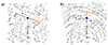 |
Fig. 1. Sketch of gravitational accelerations for two different situations. The panels show a massive body (blue dot) orbiting among stars, and the system’s barycentre at the bottom is the focus of the global gravitational acceleration gcm (open circle). The mean field acceleration gives rise to a velocity component δv• along the vertical y-axis. In panel (a), a massive perturber moves at some velocity v• in an isotropic field of stars; the result of the polarisation of the stellar orbits is a net dynamical friction force a∥, parallel but in the opposite sense to v•. In panel (b), the massive body is ejected from the origin at a velocity δv• pointing upwards. It orbits in a strongly anisotropic (rotating) stellar field and slows down due to the steady negative acceleration gcm. However, dynamical friction now contributes two terms, one a∥ as before, and a second one, a⊥, orthogonal to δv•. That non-zero component due to the streaming stars causes a steady transfer of angular momentum to the perturber. We refer to this second component as dynamical traction acting on the perturber. |
 (2)
(2)
with the background stars of density ρ⋆ adding to a mass inside the orbital radius, M(< r), much larger than the massive body, M•. We also introduced a definition of the dynamical time, tdyn. (In numerical applications, the ratio Δtfric/tdyn ≃ 3; see Sect. 4.)
The type of kinetic energy diffusion that results from (1) is drawn from summing over non-resonant star-BH hyperbolic encounters. The unperturbed stellar trajectories are straight lines and vanish to infinity after the encounter with the perturber. In reality, the host galaxy spawns a finite volume, and stars with a similar orbital energy visit each other and the perturber BH repeatedly. This causes resonant coupling between the orbits when their period ratio is commensurate (Binney & Tremaine 2008). Such a resonant response leads to efficient energy exchanges and the notion of buoyancy and core-stalling (Read et al. 2006; Banik & van den Bosch 2022; Kaur & Sridhar 2018). We revisit this subject briefly in Sect. 7. In the next paragraph Sect. 3, we outline the coupling between the BH orbit and the background stars based on the non-resonant Fokker-Planck treatment.
3. Position of the problem
To achieve our goal, several simplifying assumptions are required. The first is that a well-defined galactic rotation pattern is in place. We also presume that the BH has already bound to the host system (no dissipative terms, no gas) and remains embedded in the rotating flow of stars. Also, the BH is a small fraction of the total mass (less than 1% of the stellar disc, but ≈0.1% of the system, in line with observational trends; Kormendy & Ho 2013) and much more massive than the background stars. The problem then is to identify a small set of initial conditions for the BH’s orbit that are idealised yet useful to our analysis.
3.1. Orders of magnitude calculation
Let a BH sit at rest at the origin of coordinates surrounded by a spheroid of stars drawn from a distribution function f(E, Lz), where E is the energy and Lz the z-component of the angular momentum. For simplicity, we lump together the undressed BH mass and the stars strongly bound to it (when stellar orbits evolve adiabatically in the BH potential, e.g., Binney & Tremaine 2008; Spitzer 1987, Sect. 2.3). The stars give rise to an axi-symmetric potential Φ(R, z) and the whole system is in equilibrium (à la Tremaine et al. 1994). In the context of a young galaxy in an advanced stage of formation, some sub-structures of significant mass may still induce time-dependant perturbations in the global potential. We set the BH in motion through an m = 1 perturbation mode, which we model as a hyperbolic (shock) encounter with a body of mass Mp, impact parameter p, passing by the BH at velocity Vp parallel to the z-axis (Spitzer 1987, Sect. 5.2). The velocity imparted to the BH is then
 (3)
(3)
with a velocity vector, δv•, that we align with the y-axis of a Cartesian frame of reference (see Fig. 1[b]). When the (dynamically hot) spheroid of stars spawns a uniform density ρ⋆, the orbital motion is flagged with a reference angular frequency  , and the amplitude of the BH orbit can beestimated from the solution for a harmonic oscillator,
 (4)
(4)
The impact parameter, p, and the relative velocity, Vp, in Eq. (3) are free for us to choose. However, the mass, Mp, can be constrained by requiring that the perturbing body survives the encounter. For an extended body (such as a clump of gas or a star cluster), this will be achieved if Mp exceeds the local Jeans mass (Binney & Tremaine 2008, Sect. 3):
 (5)
(5)
In this equation the length λJ is the Jeans wavelength and σ⋆ is the stars’ one-dimensional velocity dispersion. A massive BH will generate a strong tidal field in a volume where it contributes much of the mass; furthermore, the impact parameter, p, should be greater than the size of the perturbing body, Mp; otherwise, it could overlap with the BH at the closest approach. For these reasons, in numerical applications we set
 (6a)
(6a)
![Mathematical equation: $$ \begin{aligned} l_\bullet \equiv \left[ \frac{3}{4\pi }\, \frac{M_\bullet }{\rho _\star } \right]^{\,\displaystyle {\frac{1}{3}}}\, \end{aligned} $$](/articles/aa/full_html/2025/09/aa53104-24/aa53104-24-eq9.gif) (6b)
(6b)
for self-consistency. The length l• is sometimes referred to as the BH radius of influence (as in Merritt 2004 up to a factor 2; l• should not to be confused with the event horizon of relativistic gravitation).
We considered a naked BH mass but included all stars with a binding energy (to the BH) exceeding the energy perturbation applied to the BH itself. For stars in a quasi-Keplerian orbit around the BH, this rough approximation implies that the BH mass includes stars confined to a Bahcall & Wolf (1976) cusp where ρ⋆ ∝ r−7/4. We discuss the implications of this simplification in the closing section (Sect. 8). Below we derive expectations from a Fokker-Planck treatment of the diffusion of kinetic energy. Mathematical details can be found in Appendix A.
3.2. Sample distribution function
A Fokker-Planck treatment requires a choice of the phase-space distribution function f(x, v). We applied a Dirac δ-function to select loop orbits otherwise drawn randomly from f. The distribution function (d.f.) takes the form
 (7)
(7)
where R, ϕ, and z are cylindrical coordinates; Ω(R, z = 0) is the local angular frequency; and  is the one-dimensional Dirac operator (with units of v−1; see e.g. Fukushige & Heggie 2000; Renaud et al. 2011, for further applications of the Dirac operator). The R, z components of the velocity field are made to be irrotational and isotropic by fixing
 (8)
(8)
We set the azimuthal velocity component of the BH, vϕ, equal to the parallel component, v∥, in Eqs. (A.3a-c), so

throughout. This will prove sufficiently accurate to recover the evolution with the restricted N-body numerical models of Sect. 4.
With the definition
 (9)
(9)
and the help of Eqs. (A.3), (A.6) and the relations (7) and (8), we found
![Mathematical equation: $$ \begin{aligned} \langle \Delta v_\phi \rangle = \Gamma \frac{M_\bullet }{m_\star }\frac{v_\phi }{v}\, f_\bot (0) \left[ \mp 2\pi + x e^{x^2} \, \mathrm{erfc} (x) \right] \times \frac{\mathrm{d} \mathcal{K}}{\mathrm{d} v} , \end{aligned} $$](/articles/aa/full_html/2025/09/aa53104-24/aa53104-24-eq15.gif) (10)
(10)
where  and erfc(x) is the complementary error function. The key feature of Eq. (10) is that the contribution to the variation in kinetic energy vϕ ⟨Δvϕ⟩ changes sign with RΩ − vϕ (see Eq. [A.7]). It is the exact same feature of gain or loss of kinetic energy depending whether the orbit trails or leads a resonant density pattern, as found in earlier studies (Tremaine & Weinberg 1984; Rauch & Tremaine 1996; Weinberg 1989; Kocsis & Tremaine 2015). We do not treat the growth of resonant features here, as we focus only on the response of the background stars and its impact on the BH’s orbit.
3.3. The transition to dynamical traction
Figure 2 plots the rates of specific kinetic energy variation entering the right-hand side of Eq. (A.7) as function of the azimuthal velocity component, vϕ. For the reference calculations displayed on Fig. 2(a), the Coulomb potential was set to lnΛ = 21 (N = 105) and m⋆ = 1.6 × 10⁴ M⊙, M• = 1 × 10⁷ M⊙; the rotational velocity RΩ ≃ 70km s1 at cylindrical radius R = 1.5kpc fixes the angular frequency. Two sets of results are shown, obtained for a stellar velocity dispersion σ⋆ = 10km s1 (in blue) and 20km s1 (in black).
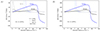 |
Fig. 2. Rates of specific kinetic energy diffusion, ⟨ΔE⟩, as a function of the azimuthal velocity, vϕ. The rates are evaluated from Eqs. (A.7) and (A.3) for two values of the stellar velocity dispersion, σ⋆ : 20km s1 (in black or grey); and 10 km s1 (in blue or skyblue). A) Setting M• = 1 × 10⁷ M⊙, with M•/m⋆ ≃ 103, the figure graphs each quadratic component and the first-order parallel one (v∥ ⟨Δv∥⟩, dark solid lines; we note that it has the same sign as RΩ − vϕ). B) The same but for a BH with M• = 1 × 10⁸ M⊙ (M•/mstar ≃ 104). The much higher inertia of the BH leads to a ten-fold increase in the parallel term but only subtle differences in the diffusion (quadratic) ones. The light and dotted-blue curves peak off scale in either case. The (central) angular velocity Ω = 0.05/Myr is such that RΩ ≈ 70km s1 at R = 1.5kpc, a good match to the circular velocity at that radius. |
The high sensitivity to σ⋆ is clearly visible for the quadratic terms ⟨(Δv⊥)2⟩ and ⟨(Δv∥)2⟩. With σ⋆ = 10km s1, both curves rise steeply at low vϕ, and reach a maximum value well off-scale on the figure. Thus at low vϕ, the gain or loss of kinetic energy is completely dominated by random scattering. The expectation, therefore, is that unless the BH is on an orbit with a significant azimuthal velocity, it is unlikely to acquire further streaming motion. Instead, a gain in radial and vertical velocity would set it on a new orbit of increased eccentricity (no gain in angular momentum) at a different energy, E. The turnover from a gain in radial- to one in azimuthal kinetic energy occurs at vϕ ≈ 45km s1, when the rate  reaches a much larger amplitude than the quadratic terms. By contrast, when the velocity dispersion σ⋆ = 20km s1, the rates ⟨(Δv⊥)2⟩ and ⟨(Δv∥)2⟩ peak at a much lower value of vϕ ≈ 6km s1, and decrease rapidly thereafter. The gain in azimuthal kinetic energy becomes dominant at vϕ ≈ 20km s1 and larger values, which translates in a net gain in azimuthal motion from that point on-ward. This behaviour is expected because a warmer stellar population will be harder to polarise, and so the effect of random scattering off of the BH orbit is much reduced (less effective gravitational focusing). The streaming flow remains the same, however, so the response in azimuth is much less affected by variations in σ⋆. We say that the gain in angular momentum is triggered by a dynamical traction transition1 because for some critical value of vϕ, the orbit of the BH gains angular momentum systematically, transforming its orbit from a low-Lz box orbit to a high-Lz loop. The onset of this seemingly irreversible trend is a sensitive function of the velocity field of the background stars. We cover this point more fully with applications later in Sect. 3.5.
Another important parameter is the choice of BH mass. On Fig. 2(b), we graph the results for the same 1D velocity dispersions σ⋆, for a BH of mass M• = 1 × 10⁸ M⊙. The ten-fold increase in M• means that the rate v∥ ⟨Δv∥⟩ also increases ten times (see the multiplicative factor in Eq. [A.7]). The most noticeable effect is a slight shift to the left of the curves for ⟨(Δv⊥)2⟩ and ⟨(Δv∥)2⟩, which both cross the run of v∥ ⟨Δv∥⟩ at lower values of vϕ. For example, for the case with σ⋆ = 20km s1 the turnover to a regime where v∥ ⟨Δv∥⟩ is dominant takes place at vϕ ≈ 12km s1 (it was ≈20km s1 on Fig. 2[a] for the lower-mass BH). This suggests that the more massive BH may yet gain angular momentum from a more slowly rotating stellar flow (all other quantities being unchanged). To back up this intuition, we have checked that reducing the angular frequency Ω from ≈7.0 × 10⁻¹ Myr−1 to 3.5 × 10⁻¹ Myr−1 brings the crossover value to vϕ ≈ 20km s1, when σ⋆ = 10km s1; and to vϕ ≲ 5km s1, when σ⋆ = 20km s1.2 The crossover value goes down by a factor of more than two from the reference calculation, highlighting the strong link with the rotation curve. The calculations with the reduced angular speed Ω still had a circular velocity ≃35km s1 at R = 3/2kpc, significantly larger than the two values for the velocity dispersion σ⋆ that we tested. A reduced Ω implies longer timescales for the onset of the dynamical traction transition (i.e. when the net gain in angular momentum will exceeds the loss to dynamical friction, and transform the orbit of the BH to a loop orbit).
There is no gain or loss in azimuthal energy from dynamical traction when vϕ = RΩ (co-moving BH) because v∥ ⟨Δv∥⟩=0 there. In the event of the BH running ahead of the stars, the rate v∥⟨Δv∥⟩< 0 changes sign. If and when that is the case, the BH loses kinetic energy and angular momentum, when it was gaining before. This is the signature of an 1:1 resonant trapping at co-rotation. That result was obtained by an argument of symmetry, rather than a proper linear perturbation treatment of the stellar response. No such analysis was needed here because we focused on the perturber (the BH) and not the system as a whole.
3.4. Time evolution
A self-consistent treatment of the orbital evolution of the BH with diffusion coefficients would require a full 2D Fokker-Planck integration. The configuration we are treating is far for equilibrium and will evolve on a dynamical timescale. For that reason, we make more progress with a set of restricted N-body integrations (see Sect. 4). Here we focus on the linear and diffusion terms of Eq. (A.7) to compute the increase in kinetic energy of each parallel and orthogonal degrees of freedom by treating their independent evolution. With this rough treatment we can estimate quantitatively the timescale over which the dynamical traction becomes dominant and the BH acquires significant angular momentum, Lz.
The specific kinetic energy Ek of the BH is a sum over quadratic components of the velocity v2 = v∥2 + v⊥2. We split Ek = E∥ + E⊥ such that
 (11)
(11)
 (12)
(12)
We computed e.g. E⊥ from Eq. (A.7) with a simple summation over time; likewise for the two components of E∥. For instance,
By assuming that the diffusion terms always have the same (positive) sign, we optimise the growth of kinetic energy orthogonally to the rotation flow. Since the flow of rotating stars singles out the torque acting on the BH, we argue that this approach slows down the transfer of angular momentum to the BH because the BH would take longer to develop a velocity vector that runs parallel, or nearly parallel, to the flow of stars.
To avoid a singularity in the diffusion coefficients, we set up the BH with a small velocity vector such that v∥ = v⊥ ≃ 3km s1 initially at a cylindrical radius R = 1.5kpc; we also set σ⋆ = 15km s1 in Eq. (8) to boost the growth of velocity components (dispersion and stream; see Fig. 2). The results of the integrals over time are displayed on Fig. 3 for a BH of mass M• = 1 × 10⁷ M⊙, with a ratio M•/m⋆ = 103. The initial rapid growth of the velocity dispersion components σ∥ or ⊥ is clearly visible, but we note how it quickly levels off as the BH velocity increases (large relative velocities diminish the efficiency of energy diffusion). On the other hand, the component parallel to the stellar flow, i.e. v∥ = vϕ, reaches a larger amplitude than either of the two dispersions σ∥ or ⊥ after ≈270 Myr of evolution. The square streaming velocity, v∥2, of the BH soon exceeds the sum of the two squared dispersion components σ⊥2 + σ∥2 at times t ≃ 300 Myr (see Sect. 3.5 below). In other words, there is more specific kinetic energy in the streaming motion (carrying angular momentum) after 300 Myr of evolution. This is close to three full periods of ≃95 Myr at a distance R = 1.5kpc and with a rotation flow RΩ = 100km s1. Not surprisingly, perhaps, this coincides exactly with the estimated time to dissipate kinetic energy in isotropic systems given by Eq. (2). But where one effect drains out orbital energy, the traction mode opposes this trend.
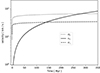 |
Fig. 3. Amplitude of the BH velocity components as a function of time. The figure graphs the velocity dispersion for each parallel and orthogonal component (denoted as σ∥ or ⊥ in the legend) and the (first-order integrated) streaming velocity (v∥, black solid line). The period of a circular orbit at radius R = 1kpc (1.5kpc) is ≃61 Myr (95 Myr). |
3.5. The onset of the transition to dynamical traction
As seen from Fig. 3, at some point in time the BH acquires a velocity vector such that its main component is vϕ ≈ v∥ so that it moves almost (though not exactly) in the direction of the flow of stars. Its z-component angular momentum Lz = Rvϕ also increases with time. We stress that the time integral that we performed did not take into account any motion in R or z. Despite this caveat, it is interesting to predict when the growth of angular momentum through the transition to dynamical traction must set in and transform the BH orbit into a loop orbit. We define this turning point as the value of vϕ such that the rate v∥ ⟨Δv∥⟩ exceeds the sum of the rates due to the diffusion terms (see Fig. 2). We find that turning point for M• in the bracket [105, 109] M⊙ and plot the results for four values of the stellar velocity dispersion σ⋆. We look at a few cases more closely below.
3.5.1. Example for an M• = 107 M⊙ BH
The outcome for that case is shown on Fig. 4. Consider the case of a BH with M• = 107 M⊙. At low values of vϕ, the BH gains and looses velocity components isotropically from the background stars. The gain and loss of such increments acquired stochastically mean that we do not expect a net increase in angular momentum, and the configuration is deemed stable. If and when the BH has acquired a significant azimuthal component, however, the situation changes. When σ⋆ ≃ 70km s1 and vϕ ≥ 7km s1, the positive transfer rate v∥ ⟨Δv∥⟩ noticebly exceeds the other terms, and hence vϕ will continue to grow. Thus as the M• = 107 M⊙ BH crosses the dotted line in Fig. 4, the system switches from a stable to an unstable configuration. The physical reason for this is that the BH continues to induce a response in the stellar density as described originally by Chandrasekhar (1943), whereas the weak response coming from the quadratic diffusion coefficients only becomes weaker as the motion of the BH aligns with that of the flow of stars. (To first order one has ⟨Δv⊥⟩=0 by symmetry, which is exact if we set vϕ strictly equal to v∥.)
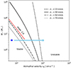 |
Fig. 4. Critical line of stability for various configurations. The vertical axis is the BH mass M• plotted against azimuthal velocity vϕ. At fixed M•, the minimum azimuthal velocity vϕ to reach such that the dynamical traction sets in is found by crossing one of the black curves, from left, to right. Four curves are plotted, each corresponding to a different value of the stellar velocity dispersion σ⋆ as indicated in the legend. The blue dot marks the estimated coordinates of the Milky Way’s BH. The red curve highlights an asymptotic trend of slop ≃ − 2 found in the limit of low vϕ. |
When the stellar velocity dispersion, σ⋆, is reduced, a BH triggers a response from a wider range of stellar orbits. Consequently the stochastic evolution of the BH’s orbit persists until a larger azimuthal velocity component is reached and the transition to a systematic increase in Lz takes place. As an example, when σ⋆ is reduced from 70 to 30km s1, we find that the transition occurs at vϕ ≈ 35km s1 (solid line on Fig. 4). If we fix σ⋆ = 50km s1, the transition point shifts back to vϕ ≈ 15km s1. A similar interpretation follows from increasing the mass M• at constant σ⋆. A more massive BH will trigger a strong linear response from the flow of stars and will thus acquire angular momentum steadily even if it is surrounded by stars of a relatively high velocity dispersion.In contrast, if the stellar velocity distribution function is very cold (low σ⋆), a BH would trigger a strong response out to a large radius, in all directions. In that situation, it would not undergo a steady growth of its angular momentum unless it is given a large azimuthal velocity, for example, from an external perturbation. The shift over to a critical value of vϕ is sketched with an arrow on Fig. 4.
3.5.2. The case of the Milky Way BH
We have indicated with a large blue dot on Fig. 4 the position of the Milky Way’s BH at M• = 4 × 10⁶ M⊙ and with a velocity in azimuth ≈2km s1, an upper limit for the velocity of Sgt A* in the Galactic frame of reference (Reid & Brunthaler 2004). The situation is complicated by the presence of a nuclear cluster of stars (NSC) around the BH (Neumayer et al. 2020 for a review). Chatzopoulos et al. (2015) estimate the half-light radius of the NSC at ≃7pc, where the velocity dispersion is on the order of 35km s1. Their modelling of the NSC suggests significant rotation, with an isotropic rotator model (Binney & Tremaine 2008) of angular frequency3 . Despite the high NSC angular velocity, the mean azimuthal velocity vϕ ≃ 0.8 σ⋆ ≃ 28km s1 for the stars inside the half-light radius (Neumayer et al. 2020). The solid line on Fig. 4 gives a critical azimuthal velocity vϕ ≈ 40km s1 for a stellar velocity dispersion σ⋆ ≃ 35km s1. This is significantly larger than the measured rotation for the stars. In conclusion, the BH would not suffer a dynamical traction transition even if it had acquired a vϕ of the same amplitude as that of the stars. The ratio vϕ/σ⋆ ≃ 0.8 implies that the NSC is nearly isotropic in velocity space, so the BH would sink back to the origin quickly (Chatzopoulos et al. 2015).
That line of reasoning follows from experience with fully isotropic velocity distribution functions, f(E). For that case a massive body always loses momentum (Binney & Tremaine 2008). Consider the estimated mass of the NSC’s stellar population at ≈9 × 10⁶ M⊙, which exceeds that of the BH itself only by a factor ×2. If we apply an m = 1 perturbation to the BH, its motion would trigger a strong response from the NSC stars and bring back the BH to the barycentre on a short mass-segregation timescale given by
 (13)
(13)
with tr denoting the two-body relaxation time and M• ≃ N⋆ m⋆/2. The NSC dynamical time is
with a half-light radius, rh, of ≈7pc and a root-mean-square velocity of ≈30km s1. (See e.g., Merritt (2013), Šubr & Haas (2014) or Panamarev & Kocsis (2022) for further details and discussion on the collisional dynamics of the NSC.)
On the other hand, the impact of the nuclear stellar disc (NSD) on a scale of ∼150pc of an estimated mass ∼109 M⊙ is much more likely to trigger a sustained transition to dynamical traction (Launhardt et al. 2002; Fritz et al. 2016; Nogueras-Lara et al. 2020; Nieuwmunster et al. 2024; (but see Zoccali et al. 2024) for a critical assessment). The dynamical timescale  equals approximately 1 Myr. With the rotation velocity of ≃50km s1 at radius r = 100pc from the Gaia survey (Gaia Collaboration 2023), we computed a period of ≃12 Myr for a circular orbit at that radius. The growth rate of azimuthal velocity displayed in Fig. 2 over several ×10 Myr would be significant. We note that the NSD has been the site of recent star formation events over times of 30 to 100 Myr (Nogueras-Lara et al. 2020), while some low-metallicity stars may be as young as 100 Myr within the central-most NSC (scale of 10pc; see von Fellenberg et al. 2022; Chen et al. 2023). These are indirect indications of past perturbation on the right timescale for the full growth of the transition to dynamical traction. We do not attempt to model the central region of the Milky Way in this contribution. Instead we present a first numerical exploration of the onset of the transition in Sects. 4 and 5.
4. Restricted N-body calculations
Recently, Kaur & Sridhar (2018) and Banik & van den Bosch (2022) studied the exchange of mechanical energy between stars and an orbiting BH analytically and with a set of numerical integrations (see also Boily et al. 2008)). These studies show how the response of stars either drains energy from or invests energy in the BH’s orbit depending on the character of the stellar orbits and their parameters such as their phase, inclination angle, and so on. We view these analyses as a strong hint that different families of stellar orbits couple to a different degree with an BH, and in particular that anisotropy in the stellar velocity field is a key ingredient to the BH’s orbital evolution. Here we borrow from Boily et al. (2008), who noted that co-planar stellar orbits couple much more effectively to the BH than those at high inclination angle (see their Sect. 5.3 and Fig. 14b). This allows for a simplification of the numerical treatment, which we lay out below.
4.1. Initial conditions
We first divided the stellar population into spherical and disc components, whereby the dynamically cooler disc component is made up of stellar orbits with an angular momentum orthogonal to the orbital plane of the BH. We froze the other (dynamically hot) stellar orbits completely. The system to evolve is made of two potentials. For the frozen potential, we picked the spherical isochrone model of Hénon:
 (14)
(14)
where a is a radial scale length and MIs is the total mass. For the live potential, we opted for an axi-symmetric Miyamoto-Nagai disc in cylindrical coordinates, R, θ, z (see Sect. 2 of Binney & Tremaine 2008),
 (15)
(15)
where we defined  ; MD is the total disc mass; and a, b are radial and vertical scale lengths, respectively. We opted to fix a = 1.5kpc in both potentials and the ratio b/a = 1/6 for the disc potential.
These potentials were combined, and their joint stellar phase-space distribution function was solved in action space with the Agama package (Vasiliev 2019). A restricted N-body realisation of the stellar disc was obtained from a Monte Carlo sampling of the joint distribution function. We noted how the response of centrophobic loop orbits subjected to the motion of a massive perturber is the strongest when they are co-planar. The root-mean square variation in mechanical energy for loop orbits reaches ≈80% of the peak co-planar value whenever their orbital angular momentum remains within ± ≈ 18° of the polar vector of the perturber’s orbital plane (see Fig. 14b of Boily et al. 2008, it becomes progressively weaker for larger inclination angles). The solid angle spawned around the pole is close to 5% of the whole sphere. An isotropic distribution function would yield orbits with angular momentum vectors covering the full sphere uniformly. The disc potential (Eq. (15)) of aspect ratio b/a = 1/6 gives rise to near-circular motion within a wedge of opening angle =arctan1/6 ≃ 9.5° for close to 85% of the orbits (the distribution function becomes progressively more isotropic as we approach the centre, within a cylindrical radius R < a; it is very nearly isotropic inside a small region bound by R ≃ b = 250pc). This sits comfortably within the solid angle for which we have estimated the orbits will respond the strongest to the perturbation. With these parameters we therefore focus on discy (nearly co-planar) orbits. We could have extracted co-planar orbits directly from the spherical isochrone distribution. Instead, we recall our motivation for more anisotropic systems in the context of a galaxy merger, or the end-state of the formation of a disc galaxy. For that reason, we chose to boost the sample of disc orbits by fixing the mass parameters in Eqs. (14) and (15) in the ratio
This increased the fraction of the disc orbits by about three times what we would have drawn from an isotropic d.f. in spherical symmetry.
A physical mass of MIs = 1 × 10¹⁰ M⊙ was chosen to match the mass of the central kiloparsec of a typical galaxy. The central atomic hydrogen density of the isochrone sphere ρIs ≃ 7.16 cm−3 is only slightly lower than that for the disc, for which ρD ≃ 8.6 cm−3. These values are roughly twice the estimated value of 3.9 cm−3 for the Milky Way at the solar radius (Bland-Hawthorn & Gerhard 2016).
4.2. Numerical integration
We performed numerical experiments using the Amμse suite of community codes to integrate the equations of motion (Pelupessy et al. 2013; Portegies Zwart & McMillan 2018). The python package Amμse v.5.2 (November 2023) offers an interface to treat each component of a system as a set endowed with its own methods and attributes. We opted to couple a live set of stars to a subset of BHs and test stars using the bridge methodology (Fujii et al. 2007; Portegies Zwart et al. 2013). A bridge easily allows one to couple a Barnes-Hut Tree integrator (Barnes & Hut 1986) and the direct-summation 4th-order accurate Hermite integrator PH4 (Portegies Zwart & McMillan 2018) to integrate the disc stars and BH orbits, respectively. Both integrators are ‘bridged’ to a frozen background potential that stands in for the extended galactic centre. The BHTREE code has a setup with critical opening angle Θc which we sat to 0.5 (down from the default 0.75), and a critical number of near-neighbours for multipolar expansion which we boosted, from the default 12, to 16 and in some cases, 32. This tactic meant that more stars were integrated with a 2nd-order accurate leap-frog symplectic scheme, whereas distant stars were integrated with a quadrupolar expansion of the stars’ potential. A large softening length l = 125pc was used for the two-body star-star interaction. We found this to be the largest value that still gives a sensible resolution of the vertical structure of the disc (scale height b = 250pc) while also allowing any Jeans-type mode of instability to be resolved. The stars-BH interactions were treated with a much smaller softening kernel where l = 10pc. The more compact kernel allowed for larger deflection angles of the stars and a accurate rendering of the BH potential (the effective size of the stellar mass elements ∼40pc, see below). The parameters used for the models and integrators are listed in Table 1.
Default parameters of the potentials and Amμse numerical integrators.
Calculations were done by sampling the disc d.f. with N = 100 000 stars, so each star has a mass m⋆ = 0.16 × 10⁵ M⊙. The BH has a reference mass M• = 1.25 × 10⁷ M⊙ for a mass ratio M•/m⋆ = 781. This takes us clearly in the galactic dynamics domain with each ‘star’ the mass equivalent of a rich open cluster of (real) stars. The disc density ρD ≃ 8.6 H/cc implies a mass inside the volume spawned by l = 125pc of 1.67 × 10⁶ M⊙, or about 100 of our model stars. We argue this makes all galactic sub-structures well resolved on a scale ∼100pc and above. The physical mass of the BH exceeds the stellar mass (by a factor ≈7.5) in a spherical volume spawned by l; hence, the influence of the BH is correctly resolved on scales exceeding ∼100pc. The dynamics of the stars is also well recovered on such scales, because their individual mass is recovered from a spherical volume of radius ≈45pc. Finally, we designed a global units converter to ensure that the Amμse integrators and the Agama module work hand in hand.
A series of test cases are presented in Appendix C. We checked that the parametric setup of the numerical integrators allow circular orbits to be recovered in the frozen potentials to a high accuracy. For a live disc component, we note that the total system angular momentum is conserved to about 0.4% accuracy for a runtime of t = 1.5Gyr, which is sufficient to monitor the transfer of the orbital angular momentum from the stars to the BH, with three significant digits. In Appendix D, we address the question of the stability of the configurations with a frozen background component.
5. Results
We proceed with the problem of an in-coming BH as outlined in Sect. 3. To keep the initial conditions close to the reference configuration of Sect. 4.2, we use the same disc/halo configuration but shift the BH to a radius a = 1.5kpc, at the edge of the core of approximately constant density (recall that the same radial scale length was used for the disc and isochrone halo). No angular momentum is given to the BH initially. The initial configuration is similar to what is depicted on Fig. 1(b), after an m = 1 mode dislodged the BH from the origin. The analysis leading to Fig. 3 did not factor in the orbital evolution (especially the radial distance, R) which must occur on a timescale ∼100 Myr for the chosen radial orbit. This zero-momentum BH orbit is an idealised case of a scenario where the BH is being accreted by the system.
5.1. The case of a warm disc
When they form in a cold disc, density waves can carry angular momentum in the same way as the gravitational focusing leading to dynamical friction. To minimise the impact of such waves, we discuss first the case of a warm disc (Table 1) which remains axially symmetric throughout the integration time (barring the response to the BH’s motion).
5.1.1. Radial orbit
For a BH set on a radial orbit in a warm disc, the orbital evolution develops significant dynamical friction early on as the BH falls from rest to the system’s barycentre. The run over time is graphed on Fig. 5 for the radius, velocity components, and Lz. One can clearly see how both the radial velocity vr and cylindrical radius R diminish during the first ∼500 Myr of evolution. This corresponds to about 4 periods of the circular orbit at the initial radius, in good agreement with the timescale given by Eq. (2). But where the dissipative friction drops in amplitude with the velocity v• (the Stokes limit), the dynamical traction exerted by the stream of stars remains steady. In fact, on Fig. 5(a), the black curve mapping the angular momentum Lz increases constantly, as does the azimuthal velocity component (solid curve in red). If the effect of dynamical friction is to kill off the radial velocity component vr, one sees that dynamical traction, on the contrary, boosts the orthogonal vϕ component steadily. Hence, the BH never reaches the centre, and in fact it begins to migrate outward as it gains angular momentum (Fig. 5[a] and [b]).
 |
Fig. 5. Case when a BH is let go from R = 1.5kpc in a (dynamically) warm stellar disc (Table 1). In panel (a), the run of Lz is shown as a black solid curve, and radial and azimuthal velocity components are shown in red. In panel (b), the cylindrical radius R and the amplitude of v• are displayed, each with their own colour-coded vertical axis. In the early stage, dynamical friction makes the orbit shrink; however, the perturber BH acquires angular momentum throughout (panel [a], black curve). Both R and v• increase systematically from t ≈ 500 Myr onward. The dotted line at the bottom is the z-coordinate bound to ±15pc. Compare with the test case displayed on Fig. C.2. |
5.1.2. Circular orbit
To determine whether the BH’s orbital evolution is correctly recovered from the Fokker-Planck treatment of Sect. A, we re-started the numerical integration but now with the BH initially set on a circular orbit (same stellar disc and setup otherwise). The expectation from Eq. (A.3) and Fig. 2 is that the BH should remain trapped at constant radius, since there is in principle no net gain or loss of kinetic energy extracted from locally co-moving stars.
The results are displayed on Fig. 6 with the same colour-coding and line styles as on Fig. 5. The expected circular orbit shows significant evolution over time, for several reasons. Firstly, large deflection-angle stars-BH encounters (collisions) lead to small but noticeable time-evolution of the BH’s radius and angular momentum during the first ∼200 Myr. This is close to two orbital periods. Collisions take place because the epicyclic motion stemming from the stellar velocity ellipsoid brings stars on and out of reach of the BH radius of influence, and this happens over a few revolutions about the centre. Secondly, the (global) reflex response of the stars to the BH’s perturbation also contributes to destabilise the BH’s orbit on the same timescale4. Further orbital evolution takes place over a longer timescale of ∼500 Myr as the BH radius varies with time in the bracket 1.3 − 1.7kpc (Fig. 6[b]). We have not explored the reasons for this behaviour in any detail. However, we note that small radial displacements will be amplified if and when dynamical traction (or, friction) takes place since it increases (or decreases) the orbital angular momentum and thus boosts the orbit’s eccentricity. Also worth noting is that the timescale of 500 Myr compares well with the time of ∼300 Myr needed to transition to an azimuthally dominant increase of kinetic energy (see Fig. 2). Our conclusion is that exact balance between dynamical friction and traction is not enough to maintain a BH on a circular orbit due to the response of the stars, first locally through strong scattering and then globally by the relaxation to a new equilibrium configuration of the system as a whole. Despite these caveats, we find no systematic and continued radial migration for a BH starting with a high-Lz orbit, in contrast with the case of initially having only radial motion.
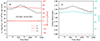 |
Fig. 6. Similar to Fig. 5 but now the BH started at R = 1.5kpc on a circular orbit. We note the sharp response of the axi-symmetric disc to the BH, which triggers radial motion. The disc adjusts to the black hole perturbation and settles progressively over several orbital times to a new equilibrium. The BH’s orbit, however, does not migrate significantly over the full integration time. Panel (a): Run of Lz (black solid curve). Radial and azimuthal velocity components are shown in red. Panel (b): Cylindrical radius R (in black) and amplitude of v• (in turquoise). The dotted line at the bottom is the z-coordinate bound to ±17pc. |
The results for these example orbits give confidence that the basic mechanics of friction/traction and transfer of angular momentum is well recovered by the numerical treatment. We also find that the amplitude of the motion and time-evolution stay well above the noise level graphed on Fig. C.2. The higher velocity dispersion of disc stars, of total amplitude ≈25km s1, exceeds the circular velocity in the BH’s potential at the linear resolution l = 125pc, for which we computed
The relative velocity between stars and the BH orbiting at the same radius (so sharing the same velocity in azimuth) may yet be high enough to prevent a significant number of stars from binding with the BH. Visual inspection of density maps suggests that only a few stars bind up with the BH. That situation will change when the BH orbits in a dynamically cooler disc, as we argue in the next sub-section.
5.2. The case of a dynamically cool disc
We now turn to the more complex case of a cool disc, when the vertical stellar velocity dispersion is reduced to σz ≈ 4.5km s1; the disc effective scale height ≃100pc is lower by more than a factor of two compared with the warm disc (when h ≃ 240pc). Self-gravitating Jeans fragments and large-scale spirals are triggered by the BH’s gravity, which we view as an m = 1 perturbation mode. In the reminder of this section, the discussion follows the reference configuration for a dynamically cooler disc listed in Table 1 unless stated otherwise.
5.2.1. Radial BH orbit
Let the BH start from rest at R = 1.5kpc initially, as done before for the warm disc (Sect. 5.1.1). The early evolution is staged on Figs. 7 and 8, where we find the BH initially falling to the system’s barycentre due to the mean gravitational field. A full orbit is completed in ≃123 Myr. These first few orbital times show the BH triggering large-amplitude density waves, and these last for several hundred Myrs, seen both in density maps and in the velocity field (see Fig. 8). In the time interval running up to t ≃ 400 Myrs, the BH acquires significant angular momentum, as shown on Fig. 9(a), where we plot the z-component of L = M• R• × v• along with the radial and azimuthal components of v•. At t = 200 Myr, we compute Lz ≈ 120 × 106 M⊙kpc/km s1 or ≈20× the peak value obtained in the test calculation with initially v• = 0 (Figs. C.1 and C.2). Therefore this early evolution is not the result of numerical inaccuracies or approximations made. Furthermore, a shift in the orbital phase of the BH has no effect (Fig. 10).
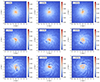 |
Fig. 7. Evolution of the system when the BH is released from rest at a radius of r = 1.5kpc (from top left to bottom right). The black arrow indicates the velocity vector. Large density fluctuations soon develop in the inner ∼1kpc where the BH potential becomes dominant. After t ≈ 100 Myr of evolution, strong density fluctuations appear, including large-scale voids (deep blue). The BH used in the calculation had a mass M• = 1.25 × 10⁷ M⊙. |
 |
Fig. 8. Transition to a fragmented morphology for a galactic disc perturbed by a massive BH. Left-hand panels: Density map of stars with peaks indicated in red. Right-hand panels: Velocity field. A black dot indicates the BH of 1.25 × 10⁷ M⊙ (or, ≃1% the mass of the stars), with its velocity vector also in black. The configurations are displayed at three different times: 144 (top), 308 (middle), and 452 Myr (bottom row) of evolution. Contour levels in yellow (left-hand panel) and grey (right-hand panel) identify the member stars of the clump formed at t = 452 Myr. The BH sits at ≃52pc of the coordinates centre. The relative velocity between the clump’s centre of mass motion and the BH is indicated with an arrow on both panels, pointing in a north, north-west direction (west is to the left). |
 |
Fig. 9. Case of a BH falling from rest on a radial orbit. a) The solid black curve graphs the angular momentum accrued over time (left-hand axis with black labels); the right-hand axis is the scale for each velocity component (red curves). b) The cylindrical radius (in black, left-hand axis) and velocity (right-hand axis, in turquoise) are shown as a function of time. The dotted line at the bottom is the z coordinate bound to ±12pc. |
 |
Fig. 10. Similar to Fig. 9 but for when the BH is launched from the origin at vy = 80km s1 and comes to rest at a radius of R ≃ 1.35kpc. The run of all quantities are remarkably similar, but for a shift in time of ≈200 Myr (≈ two orbital times) when Lz peaks. We also note that the phase of dynamical friction does not bring the BH close to the origin, as its apocentre distance always exceeds 250pc. The gain in angular momentum seen in panel (a; black curve) begins before 500 Myr. |
Despite the strong coupling and efficient transfer of angular momentum between stars and BH, dynamical friction soon takes over and drives the rapid decrease in radius, bringing the BH systematically closer to the centre (Fig. 9[b]). Specifically on Fig. 8, bottom frame when t = 452 Myr, we find the BH within r• ≃ 52pc of the centre, well below our spatial resolution limit of 125pc. At that time, it is moving at a velocity of ≈11.3km s1 in the direction of the large banana-shaped clump directly above it to the north. The phase-space coordinates of the BH are consistent with harmonic motion in the frozen background potential as depicted on Fig. C.1. However, the kiloparsec-size over-density breaks the axi-symmetry of the background potential and exerts a net pull on the BH. We wondered what impact that would have on its orbital evolution.
To investigate this, we first draw an outline of the over-dense structure with a surface density threshold of > 0.06, or four standard deviations above the mean5. We display the selection with three density contour levels on Fig. 8. Stars that fall inside that area were picked up by estimating the density at the position of each star using the same Gaussian kernel as for the gridded maps of the disc. The set of stars selected together make up a mass of 32 × 106 M⊙ (2002 member stars), or close to 2.6× the mass of the BH; we refer to this set of stars as S452. To inspect the internal cohesion of S452, we computed its total mechanical energy E = Ek + W and found E ≈ 8046.6 (km/s)2 M⊙ > 0 with a ratio Ek/|W|≳1.77 to 1.88, depending on whether the was trimmed of a subset of the most distant stars to its barycentre, or not. The positivity of the mechanical energy is robust against details of the selection procedure, and implies that the clump is not bound. An unbound over-density should be interpreted as a wake caused by dynamical friction triggered by the massive perturber (Chandrasekhar 1943; Binney & Tremaine 2008). To assess the likelihood that a subset of S459’s member stars are not, by themselves, a bound sub-system, we re-computed the energy E of each star in the rest frame of the selected clumped stars taken in isolation. We identified stars that had a negative energy, and found out that these make up 62% of the 2002 stars selected. We then removed all the stars with a positive energy and recomputed the potential of the new stellar clump with (now) only 843 stars: that system had a total positive energy, with a kinetic- to gravitational energy ratio very close to Ek/|W|=1.40. The conclusion we draw from this analysis is that self-gravity plays only a minor role in the interaction of the clump with the BH, because unbound stars contribute a too-important fraction of the clump’s gravitational potential.
S452 member stars disperse progressively over a timescale of ∼200 Myr, close to two orbital periods, somewhat slowed down by their own gravity. We ask whether the initial configuration of S452 may efficiently drag the BH out of the origin. Switching to the rest-frame of the BH, we find the clump moving away on a north, north-west trajectory at a velocity of ≃9.8km s1 (the velocity vector is displayed on Fig. 8). This configuration matches very much the m = 1 mode of perturbation discussed in Sect. 3, here on a radial scale of ≃1kpc. The distance of the centre of mass of the clump to the BH is ≃340pc, which gives rise to a monopole acceleration of GMclump/||R• − Rclump||2 ≃ 0.00131kpc/Myr2. An acceleration of this amplitude maintained for Δt ≈ 40 Myr (the dynamical timescale) would displace the BH by
That this expectation is not fully realised is seen on Figs. 9(b), where the BH orbital radius increases to a much lesser extent over ≃50 Myr of evolution. The steady, nearly linear rise of the BH’s radial distance and velocity in the interval t = 452 Myr to ≈1 Gyr seen on Fig. 9(b) instead suggests that the acceleration field applied to the BH does not remain steady, but fluctuates in amplitude over time6. In other words, the clump of stars exerting a pull on the BH certainly does not preserve enough of its mass and morphology to have a significant impact on its long-term orbital evolution. Because the size of the clump compares well with the Jeans length λJ ∼ 670pc of Eq. (D.1), we initially concluded, wrongly, that the self-gravity of the clump enhanced significantly the amplitude and duration of the traction on the BH. The dissolution of S452 argues against that.
5.2.2. The core region, fragments
The BH perturbs the core region significantly as soon as its orbital radius ≃200pc or lower, since inside that volume the mass M• compares with the total gravitational mass of stellar and frozen components. We found the velocity dispersion near the centre increasing over time to more than 20km s1 (up to a peak value of 25.5km s1 around the time t ≈ 452 Myr), distorting both the radial flow and rotation curve. A high velocity dispersion facilitates the coupling between the BH and the streaming stars (e.g. Fig. 2), because it reduces the amplitude of Brownian motion by the perturber. After the BH has reached deep in the core region, the axi-symmetry of the stellar flow is broken: we argued in Sect. 5.2.1 that a single impulse by a massive clump of stars gives enough linear momentum to shift the BH away from the centre in a region where the stellar stream becomes dominant again. The angular momentum is transferred to the BH progressively thereafter, driven by dynamical traction from the streaming stars. It is worth noting that the BH closely follows the mean disc rotation from the time t = 750 Myr onward. The BH has essentially the same specific angular momentum as the surrounding stars. After a closer look at Fig. 9(b), we noted that it shows an orbital radius oscillating with significant amplitude, and the oscillation increases as time passes. The BH is on an eccentric orbit, and the implication is that it rotates faster and then slower (in angular speed) than the stars as it shifts from the perigee to the apogee of its galactic orbit. It is therefore trapped around the radius of co-rotation with the surrounding stars (see Fig. 2 and Appendix A).
5.3. Dynamically cold discs and BH orbits with angular momentum
We turn to a more likely situation where the BH starts off on an orbit that carries angular momentum. The case of the circular orbit is the most illustrative. The radial and azimuthal velocity dispersion of the stars mean that the BH falls victim of the asymmetric drift (Binney & Tremaine 2008, Sect. 4.4, p. 326), implying a faster BH velocity in azimuth than the mean for the surrounding stars. The faster BH motion causes a net negative drag (from the stars) and a loss of angular momentum. In practice the stellar velocity dispersion is so low that the asymmetric drift causes a difference of only ∼1km s1 with circular motion, much lower still than the 1D dispersion of ≈4km s1 (see Tab. 1). We expect the asymmetric drift to have a negligible impact here.
On the other hand, a reduced stellar velocity dispersion boosts the local gravitational focusing of the stars by the BH. This phenomenon enhances the number of stars that bind with the BH. At the spatial resolution r = l = 125pc, the circular velocity in the BH’s gravitational field,
is much higher than the 3D velocity dispersion (i.e. ≈7km s1) of the unperturbed stellar disc component. A significant number of stars in the annulus R = 1.5 ± 0.125kpc will therefore interact strongly with the BH (the annulus covers close to 2.8 % of the disc’s surface but contains about 5% of the disc’s mass; the BH makes up ≃0.8% of the disc’s mass).
5.3.1. Evolution from a circular orbit
The time evolution is mapped out on Fig. 11. It is noticeable on the frames running from t = 40 Myr to 308 Myr that the BH attracts stars and "cleans up" its orbit so that a trail of low-density (a gap) forms. The bridges of higher density that form on either side of its orbit lead to the efficient angular momentum transport and orbital evolution, as in proto-planetary circumstellar disc dynamics (so-called Type-II migration; e.g., Kley & Nelson 2012; Papaloizou 2021). An importance difference is that no ram pressure exists in the disc material, and the spiral features are never close to axial symmetry. Despite these caveats, it is clear that gravitational torques acting on the BH’s orbit, rather than the net effect of dynamical traction / friction, drive this rapid inward migration: a wake of stars slowing down the BH would show up as a trailing over-density on Fig. 11, in the frames t = 61 Myr to 308 Myr. Instead we find an area devoid of stars in front and behind the BH. Compare this situation with the case of the radial orbit (Fig. 7; see also Fig. 8): clearly for that case, an over-dense wake trails the motion of the BH. The rapid evolution of the disc response over a few periods causes the clumps of disc material to interact and merge with each other, and they eventually form dense substructures with a roundish shape. This situation is depicted in frame t = 915 Myr when the BH is within 20pc of the centre. The BH is virtually at rest at that time, since its velocity v• ≃ 9km s1 lies within the numerical uncertainty for a BH starting at the centre of coordinates with no motion (Fig. C.2).
 |
Fig. 11. Evolution of the BH set on a circular orbit initially of radius r = 1.5kpc (top left to bottom right). The black arrow indicates the velocity vector. Large spiral waves and Jeans fragments develop quickly due to the lower stellar velocity dispersion. The BH binds with stars and opens a gap in its wake, which leads to a steady loss of angular momentum and inward migration. This is most visible in the frames with time running from t = 41 Myr to 915 Myr. At t = 915 Myr the BH sits at r ≈ 20pc with a rest-frame velocity ≃9km s1. Non-axi-symmetric clumps of stars dislodge the BH which acquires significant angular momentum by dynamical traction in the later stages of evolution (on a timescale ∼500 Myr). Calculations performed with a BH of mass M• = 1.25 × 10⁷ M⊙. |
It is important to note that the fragmented mass density at t = 915 Myr breaks the axi-symmetry of the system. A direct consequence of this is that the BH does not remain still, but is pulled out of the origin by one large clump, or a few small ones. The energy and angular momentum gained by the BH means that by t = 1553 Myr, it is now orbiting at a radius R ≈ 300pc; it has acquired significant angular momentum which persists until at least t = 1750 Myr, when the disc material defines a bar-like potential on a scale of ∼500pc (the BH radial orbit is then at a radius ≃710pc). The run of radius, velocity components and angular momentum is plotted on Fig. 12. It is striking how the angular momentum drops to essentially zero at t ≈ 915 Myr, and rises systematically thereafter. The same comment applies to its orbital radius, seen on Fig. 12(b). The fact that the BH’s orbit does not circularise exactly (small but persistent oscillations in radius R) may be one reason why symmetry breaking is enhanced near the origin, i.e. on a scale matching the BH’s radius of influence,or r ≈ 300pc.
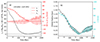 |
Fig. 12. Runs of angular momentum, radius, and velocity components as a function of time for a BH started on a circular orbit. a) The solid black curve graphs the angular momentum (left-hand axis with black labels). The right-hand axis is the scale for each velocity component (red curves). b) The cylindrical radius (in black, left-hand axis) is graphed together with the norm of the velocity (right-hand axis, in turquoise). The dotted line at the bottom is the z coordinate bound to ±10pc. The radius and velocity components reach a minimum at t = 915 Myr. |
5.3.2. Eccentric orbits
To underscore the singular character of the (initially) circular BH motion, we ran two more cases with the BH starting on mildly eccentric orbits. On Fig. 13, we display the runs of orbital angular momentum Lz (panel [a]) and radius (panel [b]) for the initially circular orbit discussed above (e = 0), along with two orbits that begin with lower Lz. The first one has Lz → 5Lz/6 leading to an orbit of small eccentricity (e ≈ 0.55); the second one has Lz reduced by a second factor 5/6 so Lz → 0.7Lz compared to circular motion, and a larger orbital eccentricity (e ≈ 0.67). We estimated the eccentricities from the ratio of radii at peri- and apo-centres.
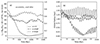 |
Fig. 13. Runs of angular momentum and radius for three BH orbits: circular; an elliptical orbit with a small eccentricity, e ≈ 0.55; and a third case with a large eccentricity, e ≈ 0.67. a) Run of the angular momentum for each case as indicated in the legend. The solid black curve graphs Lz for the circular initial orbit displayed on Fig. 12. b) Cylindrical radius as a function of time for the same three cases. We note how the BH orbit with the more elliptical orbit actually evolves at a near-constant mean radius. |
To understand the trends in Lz and radii over time, it is useful to think in terms of epicyclic motion. In this regime, the angular momentum is conserved as the object moves in and out radially. We may assume that this is true of the unperturbed stellar orbits. Here, the BH may dominate the gravitational potential locally and polarises stellar orbits of lower and higher Lz, inside and outside of its orbit, respectively. When the BH starts off on a nearly circular orbit, its own epicycle does not generate significant radial motion compared with the radial stellar velocity dispersion  . Thus in the limit of small e, the BH act as a gravitational focal point. It is able to open a gap along its orbit, when it becomes a catalyst for angular momentum transfer, from the stars inside its orbit, to the stars outside it. This is a very similar situation to the instability studied by (Julian & Toomre 1966) for a thin, cold fluid of stars. On the contrary, when the BH is launched from a low-angular momentum orbit, of higher eccentricity e, it is unable to clear a gap in the stellar population because its own significant radial motion effectively boosts its velocity relative to the stars. This in turn makes the BH a less effective gravitational attractor. The BH orbit labelled large e ≈ 0.67 on Fig. 13(b) gives a mean-amplitude (rms) radial velocity of vR ≃ 6.8km s1 which is in fact larger than the stellar radial velocity dispersion, at least initially. Hence the BH stops being a point of gravitational focusing, and fewer stars respond strongly to its gravitational pull. A gap does not form, and the BH orbit preserves its angular momentum more efficiently.
5.4. Transition from gravitational torques to dynamical friction
Our study of BH orbital evolution points to a more complex picture than for warm discs. The time evolution of a BH orbit initially with zero angular momentum is first driven by dynamical friction in competition with dynamical traction (see Sect. 5.1.1). This happens both in a dynamically warm- or cold stellar disc, and can lead to a transition, from a contracting orbit losing angular momentum, to an expanding orbit gaining angular momentum. When the disc is cold and the BH starts on a near-circular orbit, the mechanics at play is not that of dynamical friction because a massive body will suck in stars that are close in phase-space: the formation of a gap of under-dense regions stretching in front and behind the massive body is the signature of this process (Fig. 11). We have argued, based on two cases of BH orbits that start on mildly eccentric orbits, that gap formation shuts off if the BH is on a sufficiently eccentric orbit, and the interplay of dynamical friction / traction kicks in. This transition to an evolution of the orbital momentum driven by gravitational focusing (friction or traction) occurs at a critical orbital angular moment for fixed values of M• and stellar velocity dispersion σ⋆ (the radial component mostly controlling the Toomre stability parameter Q; see Eq. (D.2)). We have not identified a relation between Q, Lz, and M• that quantifies this transition. We anticipate that this point is worthy of a study all by itself, to which we hope to return in a future contribution. In the next section, we seek to justify in more quantitative details the application of the Fokker-Planck treatment to cold systems.
6. Comparison with theory
Our analysis of kinetic energy diffusion of Appendix A was developed with a smooth homogeneous background in equilibrium in mind. The surface density maps of our numerical cold discs models, indeed images of high-z galaxies (e.g., the GOODS survey, Elmegreen et al. (2007)), on the contrary, generally point to a complex, fragmented mass distribution in the core region visited by the BH. We limit our exploration to the case when the BH starts on a radial orbit in a dynamically cold disc (Table 1). We want to assess whether the basic picture of repeated gain and loss of azimuthal velocity is indeed at work in the later stages of evolution, when the BH has acquired angular momentum from the streaming of stars (see Fig. 2 and Appendix A).
To that end, we graph on Fig. 14 the runs of specific angular momentum Lz and azimuthal velocity vϕ as a function of the cylindrical radius R for the BH orbit displayed on Figs. 7 and 8. The rotation curve for the model galaxy is displayed in solid orange, and two phases of evolution are displayed with different colours: prior to Lz reaching a maximum (in dark blue); and at later stages when Lz decreases episodically (in red). The two phases are shifted for clarity (the light-blue dotted lines connect the end-point of one phase, to the start of the next), with large light-blue arrows indicating the flow of time. The output data was sampled at intervals of 10 Myr, from t = 1008 Myr to t = 1800 Myr, with the transition through a peak Lz value at t = 1522 Myr.
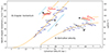 |
Fig. 14. A) Specific angular momentum, Lz, as a function of the cylindrical radius, R, during the orbital migration of the BH. The large sky-blue arrows indicate the flow of time, t. The orange solid lines trace the expected values for the model galaxy. The curve in blue (red) shows the coordinates before (after) Lz has reached a maximum. The black lines indicate evolution at a constant Lz. The circles numbered 1 and 2 single out specific phases of evolution. B) Run of azimuthal velocity, vϕ, against radius, R. The axes have been shifted for clarity. The colour-coding for the other curves and symbols is as for (A). |
We discuss first the early phase, from 1008 to 1522 Myr (dark blue curves). Fig. 14(a) graphs continued increase in Lz with time, despite significant fluctuations (positive or negative) in radial migration. Let us focus on a time slice around the coordinates marked with the circled number ❶. Near the symbol ❶, the steady increase in Lz is evident as the radius increases from ≈1.2 to 1.5kpc; notice how Lz (in blue) sits above the expected value (orange curve) at R ≈ 1.2kpc. Consider now the evolution of vϕ over the same interval, where we find again that the BH has excess azimuthal velocity at R = 1.2kpc, sitting above the orange curve. Its larger azimuthal velocity means that it jumps ahead of the stars, which exert a negative acceleration on it. Therefore, vϕ decreases in absolute terms as we move forward in time toward a larger radius R. The evolution at constant Lz would make vϕ drop and fall on a path parallel to the black straight line, which is clearly not the case (Fig. 14[b]). In fact, the azimuthal velocity still decreases such that it crosses the orange curve, and soon the BH has a significant deficit of azimuthal velocity (dot-dash blue line, near ❶ on the figure). The situation is now reversed, with the BH lagging behind the stellar flow at that radius: the dynamical traction exerted by the stars now pulls it forward and it soon catches up and overtakes the stellar flow. This see-saw pattern repeats itself up to R ≈ 1.8kpc which is near the point where the rotation curves flattens off; we find for our model galaxy that dvϕ/dR < 0 when R ≳ 2kpc, off-scale on Fig. 14(b).
The second time slice of interest is marked with the circled number ❷. In this later stage, the orbit evolves differently, with episodic loses of angular momentum, followed by time intervals of near-constant Lz. This is illustrated most clearly near the points ❷ on Fig. 14(a), when the horizontal black line (of constant angular momentum) traces well the orbit of the BH; in (b), the case of the azimuthal velocity, the black curve as a slope matching that of the data, in red. It is interesting to observe that the time intervals of near-constant Lz are close to one full orbital time, or ≈100 Myr. We suspected that this could be an indication of a bar-like structure or some other non-axisymmetric density fluctuations developing inside the BH’s orbit. But the much increased radial stellar velocity dispersion, now exceeding σR ≈ 18km s1 close to R = 0kpc (it started at 4.2km s1) works against bar- or any substructure formation. A casual inspection of density maps, not shown here, instead suggests that at the BH’s orbit of R ≈ 1.7kpc where σR ≈ 8km s1 is much lower, the BH is still able to open a gap (albeit of low contrast) in the stellar distribution. In other words, the drop in angular momentum is most likely caused by gravitational torques, which here again work to lower its orbital angular momentum. We have not investigated the duration of such torques or their net impact quantitatively but suspect that they account for episodes of rapid angular momentum loss. By contrast, a steady decline in Lz would be attributable to dynamical friction. This interpretation implies that the time-evolution of the BH’s orbit is coupled to both the inner and outer disc stellar populations through their velocity dispersion, i.e. their local stability to Jeans modes of fragmentations. A future study with spectral analysis should provide a more definitive diagnostic of angular momentum transport in these systems.
A related question which sheds light on the analysis is whether the time derivative ⟨Δv∥⟩ obtained numerically matches the values computed from Eqs. (A.3) and (A.4). We tailor these equations to the numerical setup by fixing Ns = 1 × 10⁵ and m⋆ = 1.6 × 10⁴ M⊙. We chose to round up the ratio M•/m⋆ from 731, as for the curves displayed on Fig. 2, to ≃103. This simplifies the algebra and is of little consequence to the outcome. We also set  for the two-dimensional velocity dispersion. All quantities can be expressed in units of (km s1)2/ Myr with a single multiplicative constant. In the case of σ⋆ = 10km s1, we read on Fig. 2 a value of

when v∥ ≃ 60km s1. This velocity component can also be read off Fig. 9(b) in the time interval > 1000Myr. If we isolate for ⟨Δv∥⟩ from the above relation, we find that  . A naive time-integration over the sampling interval dt = 10 Myr leads to Δv∥ ≈ 6.6km s1. Inspection of the output logs from the numerical integration gives us typical time-variations Δvϕ ≈ 4 to 5km s1, over the same time interval. In the case when σ⋆ = 20km s1, the same exercise leads to
  and Δv∥ ≈ 1.66km s1 (same sampling rate). Thus we conclude that the analytical rates in Eq. (A.3) are of the right amplitude, but they fall short when the dispersion, σ⋆, increases significantly above 10km s1. Inspecting the runs for times t ≥ 329 Myr we found a steady radial decrease in σ⋆ in the interval R = 0 to 2kpc, when σ⋆ falls from ≥20km s1, to ≈10km s1. In other words, the variations in Δvϕ become larger as we move outwards since locally σ⋆ is reduced. This comforts the conclusion that dynamical traction accounts quantitatively for much of the outward orbital evolution of the BH.
7. Discussion
The problem of a massive perturber evolving in cored galactic potentials was revisited here with a focus on a background of stellar orbits with non-zero streaming motion drawn from a simple distribution function. A local treatment of gravitational focusing derived from Fokker-Planck diffusion coefficients was performed. The effects of resonant motion was left out of the analysis. A consequence of anisotropic gravitational focusing, we argued, is that the steady streaming of stars leads to an effective traction on the BH after a few orbital periods (see Appendix A and Fig. 3). Dynamical traction competes with the more familiar Chandrasekhar friction and we have illustrated the transition from one regime to the other for a BH on a radial orbit in a hot disc (Fig. 6). This is the expected evolution for low-angular momentum BH orbits.
Theoretical expectations are largely fulfilled in configurations where the streaming stars are stable against Jeans fragmentation modes (dynamically hot discs). This is not so with cold discs, where we found that stellar sub-structures are key players in the orbital evolution of the BH. Indeed stellar clumps shut out dynamical traction almost entirely, so a BH may reach the galactic centre on a timescale of ∼300 Myr (compare Figs. 6 and 9). In this idealised framework, the formation of stellar clumps is triggered by the response of the stellar orbits to the migrating BH (no clumps form when the BH is at rest at the origin: Fig. C.1). Thus when the BH reaches the centre, the stellar mass distribution is far from axial symmetry. The configuration will be unstable if and when sizeable clumps orbit near the centre. We spoke of a two-stage instability whereby an m = 1 mode pulls the BH out of the centre, at which point dynamical traction boosts its angular momentum and outward migration ensues. Hence the degree of binding energy of these clumps (their internal cohesion, not resolved properly in our numerical integrations) is crucial to the stability of the configuration. We address this specific point below.
7.1. Fragmentation and self-gravity
Fragments that develop through Toomre-unstable ‘cold’ stellar orbits in the disc triggered by the BH perturbation mimic observations of young galaxies undergoing active star formation. The extended and spherical (isochrone) component made up of ‘hot’ stellar orbits couples more weakly with the BH; we froze the spherical component for that reason in the reference numerical setup. A drawback is that the stellar clumps themselves do not exchange mechanical energy with the Isochrone potential (by polarising orbits from that component, for instance). In that way the binding energy of the clumps is enhanced artificially, and we expect that relaxing the constraint of a frozen component will change the outcome of the numerical integration significantly. From hereon, we use the name ‘bulge’ as shorthand for spherical isochrone stellar component.
To inspect the impact of a live bulge, we performed two calculations, the first with a fraction of live bulge orbits such that they match in number (and mass) those of the live disc, or 100k mass elements each; and a second run with a fully self-gravitating bulge and disc. The second run was performed with the Amμse GPU-enhanced tree code BONSAI with a total of 8.4 × 10⁶ mass elements. The model parameters and bulge/disc mass ratios are those of the standard model of Table 1. The kernel sizes for numerical integration was reduced to l = 32pc to account better for the dynamics of the clumps.
Fig. 15 graphs for each case the distribution in space of a subset of stars that form a bound sub-structure at a time when the BH has reached the centre. The run shown on the top row (a) for a partially self-gravitating bulge yielded stellar clumps of strong binding energy. The run shows how the clumps merge together and form a structure which far outweighs the BH (by 4× its mass). The large structure of ≃3318 mass elements seen at the end of the sequence hovers close to the centre of coordinates indicated with a red dot. At the end of the time sequence, we find that 90.3% of the mass elements identified as belonging to the clump are bound together. This is a prime example of the important rôle that the net clump binding energy can have on the stability of the BH’s position in the galaxy.
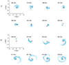 |
Fig. 15. Two examples of the interaction between the central BH and stellar sub-structures. In (A, top row), when the background spherical Isochrone potential is partially frozen, the disc stars form clumps of higher mass and binding energy. Such structures may dislodge the BH. This two-stage instability then grows as the BH extracts angular momentum from the flow of rotating stars around the centre. In (B, bottom row) the situation for a self-gravitating disc plus isochrone potential means that the clumps are much less massive and of a lower binding energy. In that case, a clump will dissolve in the strong tidal field of the BH. The centre of coordinates is indicated with a red dot. (See text for more details). |
Compare these results with the second run displayed on Fig. 15(b), where now the whole system is self-gravitating. Now some 2887 mass elements add up to ≃3.8 × 10⁶ M⊙ (1/3 the mass of the BH). The important difference is that now only about 62% of the mass of the clump has negative binding energy. As soon as it approaches the centre the tidal field of the BH dissolves the structure which forms a loose spiral pattern at the end of the run. The BH remains at the heart of the system, and may accrete stars and (possibly) form a nuclear star cluster. No instability will develop that can remove the BH from the centre unless more massive sub-structures form in the course of time: nothing of the sort happened over the course of 1.5 Gyr of evolution for that model.
These calculations tell us that if the anisotropic stellar stream is embedded in a large, much more massive hot stellar component of nearly isotropic velocity field (like the current bulge), then fragmentation modes that are triggered by a migrating BH are unlikely to develop strong biding energy and create a situation whereby the massive compact object can be ejected from the centre. The BH migrates to the centre on a timescale ∼300 Myr as anticipated from dynamical friction. We have not determined the minimum mass ratio of isotropic- to anisotropic (disc-like) components that will lead to this configuration: the calculations that we performed suggest that this ratio has to be at least 2:1. It would be interesting to extract the degree of anisotropy (essentially, rotation) from calculations of galaxy formation simulations that resolve the central kiloparsec adequately to provide a better set of constraints on the initial configuration to use for a refined study of BH migration.
7.2. Cool and warm discs
During the early stages of evolution of a low-Lz orbit, the BH undergoes dynamical friction. Two cases were considered, one where the disc is dynamically warm, the other, cool. No substructures form in a warm disc, and the evolution is very smooth (Fig. 5).
The situation is much different in cooler environments, when the disc fragments and density waves carry angular momentum outward. The BH may well sink to the centre, but be ejected by a symmetry-breaking configuration of stellar clumps which it triggered on the way in. When that happens. the BH acquires angular momentum by dynamical traction from the surrounding streaming stars. We have checked that the BH’s azimuthal velocity vϕ increases at a rate well matched with Fokker-Planck energy diffusion coefficients in that situation (Fig. 14). This is important because these coefficients are obtained from local measurements of rotation velocity, dispersion and surface brightness. Therefore the dynamical state of an off-centred BH in an external galaxy could possibly be gauged directly from a well-resolved young galaxy with a rotating bulge (or highly anisotropic bulge). Several such galaxies have long been observed at redshifts z ∼ 1 to 3 (e.g., Elmegreen et al. 2007). The recent JWST detection of an off-centre AGN at z ∼ 7.3, when the Universe is ≈700 Myr old (Übler et al. 2024), offers a great opportunity to tests and understand better BH dynamics in the early stages of the formation of a galaxy. The environment of a BH in a young galaxy should include gas dynamics and the formation of stars for a realistic diagnostic of the internal dynamics at the core of young galaxies. We stressed already how the binding energy of stellar sub-structures, surely determined by dissipation processes at formation, will impact on the stability of the BH at the centre of galaxies. Analyses of the impact of gas on the orbit of a massive perturber include, e.g., Ostriker (1999), Chapon et al. (2013) for radiative gas; and the recent work by Lescaudron et al. (2023) which includes turbulence. These last authors find a direct link between the amplitude of the turbulent power-spectrum and the orbital evolution of the BH. The density fluctuations brought by turbulent modes parallel the role played here by stellar clumps. There is a bridge to be built between such studies, because a star-forming region will proceed from gas cooling in turbulent configurations, and form large stellar aggregates (Renaud et al. 2021). It is intriguing that the BH discovered in the GA-NIFS survey (Übler et al. 2024) of an estimated mass ≃5 × 10⁷ M⊙ is offset from the host galaxy’s photometric centre by R ≃ 1kpc in projection (see their Fig. 2; the broad-line region that is clearly mis-aligned). Should the physical scales be confirmed, the BH displacement would be on the same scale as the one we found in our models. More detailed modelling is required to assess the likelihood of an event such as this, yet such observations point to a physically plausible configuration.
8. Conclusions
We have presented analytical arguments and showed with numerical N-body calculations that the mechanics of dynamical traction (see Sects. 3.3 and 5.4) work hand in hand with the classic picture of orbital decay of a massive BH derived from dynamical friction. They represent the same phenomena of gravitational focusing but have opposite effects. An anisotropic velocity field drawn from a d.f of the form f(E, Lz) may lead to a net gain of angular momentum by a massive BH and outward migration. This is true for a dynamically warm stellar velocity field. The competition between dynamical friction and traction causes a continued transition in the solution space when one effect comes to dominate over time.
A fragmented, dynamically cold configuration helps bring the perturber BH to the barycentre faster, but these very fragments make it difficult to keep it there. We identified a two-stage instability that results in outward migration of a massive BH by dynamical traction. No dissipative terms were included in our analysis, and the scale-free nature of gravitational dynamics means that all quantities of time, mass, and length can be rescaled to fit observational constraints.
Our work was focused on a galactic system of total mass =1.16 × 10¹⁰ M⊙ in equilibrium with a characteristic length a = 1.5kpc. The orbital outward migration of an M• = 1.25 × 10⁷ M⊙ BH in this system may reach ∼1kpc over a timescale of ∼750 Myr to 1 Gyr. It is noteworthy that the recent AGN identified by the JWST at redshift z ≃ 7.3 shows an offset from its photometric centre by the same length in projection (Übler et al. 2024). Ongoing and future work with fully self-gravitating calculations should shed light on the dynamics of young galaxies by resolving the core region of these fascinating systems better.
Acknowledgments
We thank the anonymous referee for a thoughtful report that led to a much improved manuscript. We acknowledge G. Monari, B. Famaey and F. Renaud for their comments and suggestions about this work. K. Kraljic also pointed out several recent papers bearing on black hole dynamics in galaxies. The research reported here made extensive use of the community projects Agama and Amμse. We thank the developers for making their software available (and documented). Part of this work was supported by the French-Ukrainian DNIPRO research grant number Ts 17/2–1 awarded in 2022. Carbon footprints: this project made use of 1680 hours of organically grown intelligence (OGI), equivalent to ∼30 kWh of energy (Balasubramanian 2021), together with 6000 CPUh of computational resources expended at the HPC centre of the University of Strasbourg (grants g2023a97-c and -g) during the academic year 2023-24. We thank M. Ringenbach and D. Brusson for support.
References
- Anglés-Alcázar, D., Özel, F., Davé, R., et al. 2015, ApJ, 800, 127 [CrossRef] [Google Scholar]
- Argüelles, C. R., & Collazo, S. 2023, Universe, 9, 372 [Google Scholar]
- Bahcall, J. N., & Wolf, R. A. 1976, ApJ, 209, 214 [NASA ADS] [CrossRef] [Google Scholar]
- Balasubramanian, V. 2021, Proc. Natl. Acad. Sci., 32, 118 [Google Scholar]
- Banik, U., & van den Bosch, F. C. 2021, ApJ, 912, 43 [NASA ADS] [CrossRef] [Google Scholar]
- Banik, U., & van den Bosch, F. C. 2022, ApJ, 926, 215 [NASA ADS] [CrossRef] [Google Scholar]
- Barnes, J., & Hut, P. 1986, Nature, 324, 446 [NASA ADS] [CrossRef] [Google Scholar]
- Barro, G., Pérez-González, P. G., Kocevski, D. D., et al. 2024, ApJ, 963, 128 [CrossRef] [Google Scholar]
- Bellovary, J. M., Cleary, C. E., Munshi, F., et al. 2019, MNRAS, 482, 2913 [NASA ADS] [Google Scholar]
- Binney, J., & Tremaine, S. 2008, Galactic Dynamics, 2nd edn. (Princeton: The University Press) [Google Scholar]
- Bland-Hawthorn, J., & Gerhard, O. 2016, ARA&A, 54, 529 [Google Scholar]
- Bogdán, Á., Goulding, A. D., Natarajan, P., et al. 2024, Nat. Astron., 8, 126 [Google Scholar]
- Boily, C. M., Padmanabhan, T., & Paiement, A. 2008, MNRAS, 383, 1619 [Google Scholar]
- Boylan-Kolchin, M. 2023, Nat. Astron., 7, 731 [NASA ADS] [CrossRef] [Google Scholar]
- Chandrasekhar, S. 1943, ApJ, 97, 255 [Google Scholar]
- Chapon, D., Mayer, L., & Teyssier, R. 2013, MNRAS, 429, 3114 [Google Scholar]
- Chatzopoulos, S., Fritz, T. K., Gerhard, O., et al. 2015, MNRAS, 447, 948 [Google Scholar]
- Chen, Z., Do, T., Ghez, A. M., et al. 2023, ApJ, 944, 79 [NASA ADS] [CrossRef] [Google Scholar]
- Chiba, R., & Kataria, S. K. 2024, MNRAS, 528, 4115 [Google Scholar]
- Chu, A., Boldrini, P., & Silk, J. 2023, MNRAS, 522, 948 [Google Scholar]
- Cole, D. R., Dehnen, W., Read, J. I., & Wilkinson, M. I. 2012, MNRAS, 426, 601 [Google Scholar]
- de Vita, R., Trenti, M., & MacLeod, M. 2018, MNRAS, 475, 1574 [Google Scholar]
- Elmegreen, D. M., Elmegreen, B. G., Ravindranath, S., & Coe, D. A. 2007, ApJ, 658, 763 [Google Scholar]
- Finkelstein, S. L., Bagley, M. B., Ferguson, H. C., et al. 2023, ApJ, 946, L13 [NASA ADS] [CrossRef] [Google Scholar]
- Fouvry, J.-B., Binney, J., & Pichon, C. 2015, ApJ, 806, 117 [Google Scholar]
- Fritz, T. K., Chatzopoulos, S., Gerhard, O., et al. 2016, ApJ, 821, 44 [Google Scholar]
- Fujii, M., Iwasawa, M., Funato, Y., & Makino, J. 2007, PASJ, 59, 1095 [NASA ADS] [Google Scholar]
- Fukushige, T., & Heggie, D. C. 2000, MNRAS, 318, 753 [CrossRef] [Google Scholar]
- Gaia Collaboration (Drimmel, R., et al.) 2023, A&A, 674, A37 [CrossRef] [EDP Sciences] [Google Scholar]
- Heggie, D., & Hut, P. 2003, The Gravitational Million-Body Problem: A Multidisciplinary Approach to Star Cluster Dynamics (IOP Publishing Ltd) [Google Scholar]
- Hopkins, P. F., & Quataert, E. 2011, MNRAS, 415, 1027 [NASA ADS] [CrossRef] [Google Scholar]
- Julian, W. H., & Toomre, A. 1966, ApJ, 146, 810 [NASA ADS] [CrossRef] [Google Scholar]
- Kalnajs, A. J. 1972, in IAU Colloq. 10: Gravitational N-Body Problem, ed. M. Lecar, Astrophys. Space Sci. Lib., 31, 13 [Google Scholar]
- Kaur, K., & Sridhar, S. 2018, ApJ, 868, 134 [Google Scholar]
- Kaur, K., & Stone, N. C. 2022, MNRAS, 515, 407 [Google Scholar]
- Kley, W., & Nelson, R. P. 2012, ARA&A, 50, 211 [Google Scholar]
- Kocsis, B., & Tremaine, S. 2015, MNRAS, 448, 3265 [NASA ADS] [CrossRef] [Google Scholar]
- Kormendy, J., & Ho, L. C. 2013, ARA&A, 51, 511 [Google Scholar]
- Labbé, I., van Dokkum, P., Nelson, E., et al. 2023, Nature, 616, 266 [CrossRef] [Google Scholar]
- Lapiner, S., Dekel, A., & Dubois, Y. 2021, MNRAS, 505, 172 [NASA ADS] [CrossRef] [Google Scholar]
- Lau, J. Y., & Binney, J. 2021, MNRAS, 507, 2241 [NASA ADS] [CrossRef] [Google Scholar]
- Launhardt, R., Zylka, R., & Mezger, P. G. 2002, A&A, 384, 112 [NASA ADS] [CrossRef] [EDP Sciences] [Google Scholar]
- Lescaudron, S., Dubois, Y., Beckmann, R. S., & Volonteri, M. 2023, A&A, 674, A217 [NASA ADS] [CrossRef] [EDP Sciences] [Google Scholar]
- Lynden-Bell, D., & Kalnajs, A. J. 1972, MNRAS, 157, 1 [Google Scholar]
- Matthee, J., Naidu, R. P., Brammer, G., et al. 2024, ApJ, 963, 129 [NASA ADS] [CrossRef] [Google Scholar]
- Merritt, D. 2004, Phys. Rev. Lett., 92, 201304 [NASA ADS] [CrossRef] [Google Scholar]
- Merritt, D. 2013, Dynamics and Evolution of Galactic Nuclei, 1st edn. (Princeton, NJ: Princeton Univ. Press) [Google Scholar]
- Merritt, D., Berczik, P., & Laun, F. 2007, AJ, 133, 553 [NASA ADS] [CrossRef] [Google Scholar]
- Mo, H., van den Bosch, F. C., & White, S. 2010, Galaxy Formation and Evolution, 1st edn. (Princeton, NJ: Princeton Univ. Press) [Google Scholar]
- Naidu, R. P., Oesch, P. A., van Dokkum, P., et al. 2022, ApJ, 940, L14 [NASA ADS] [CrossRef] [Google Scholar]
- Neumayer, N., Seth, A., & Böker, T. 2020, A&A Rev., 28, 4 [NASA ADS] [CrossRef] [Google Scholar]
- Nieuwmunster, N., Schultheis, M., Sormani, M., et al. 2024, A&A, 685, A93 [NASA ADS] [CrossRef] [EDP Sciences] [Google Scholar]
- Nogueras-Lara, F., Schödel, R., Gallego-Calvente, A. T., et al. 2020, Nat. Astron., 4, 377 [Google Scholar]
- Ostriker, E. C. 1999, ApJ, 513, 252 [Google Scholar]
- Panamarev, T., & Kocsis, B. 2022, MNRAS, 517, 6205 [CrossRef] [Google Scholar]
- Papaloizou, J. C. B. 2021, Celest. Mech. Dyn. Astron., 133, 30 [NASA ADS] [CrossRef] [Google Scholar]
- Pelupessy, F. I., van Elteren, A., de Vries, N., et al. 2013, A&A, 557, A84 [NASA ADS] [CrossRef] [EDP Sciences] [Google Scholar]
- Petts, J. A., Gualandris, A., & Read, J. I. 2015, MNRAS, 454, 3778 [NASA ADS] [CrossRef] [Google Scholar]
- Pfister, H., Volonteri, M., Dubois, Y., Dotti, M., & Colpi, M. 2019, MNRAS, 486, 101 [Google Scholar]
- Pfister, H., Dai, J. L., Volonteri, M., et al. 2021, MNRAS, 500, 3944 [Google Scholar]
- Portegies Zwart, S., & McMillan, S. 2018, Astrophysical Recipes; The art of AMUSE, IOP Astronomy/AAS (Bristol, UK: IOP Publishing) [Google Scholar]
- Portegies Zwart, S., McMillan, S. L. W., van Elteren, E., Pelupessy, I., & de Vries, N. 2013, Comput. Phys. Commun., 184, 456 [Google Scholar]
- Rauch, K. P., & Tremaine, S. 1996, New Astron., 1, 149 [NASA ADS] [CrossRef] [Google Scholar]
- Read, J. I., Goerdt, T., Moore, B., et al. 2006, MNRAS, 373, 1451 [NASA ADS] [CrossRef] [Google Scholar]
- Reid, M. J., & Brunthaler, A. 2004, ApJ, 616, 872 [Google Scholar]
- Renaud, F., Gieles, M., & Boily, C. M. 2011, MNRAS, 418, 759 [NASA ADS] [CrossRef] [Google Scholar]
- Renaud, F., Romeo, A. B., & Agertz, O. 2021, MNRAS, 508, 352 [NASA ADS] [CrossRef] [Google Scholar]
- Schawinski, K., Koss, M., Berney, S., & Sartori, L. F. 2015, MNRAS, 451, 2517 [Google Scholar]
- Spitzer, L. 1987, Dynamical Evolution of Globular Clusters (Princeton University Press) [Google Scholar]
- Šubr, L., & Haas, J. 2014, ApJ, 786, 121 [Google Scholar]
- Toomre, A. 1964, ApJ, 139, 1217 [Google Scholar]
- Tremaine, S., & Weinberg, M. D. 1984, MNRAS, 209, 729 [Google Scholar]
- Tremaine, S., Richstone, D. O., Byun, Y.-I., et al. 1994, AJ, 107, 634 [CrossRef] [Google Scholar]
- Übler, H., Maiolino, R., Pérez-González, P. G., et al. 2024, MNRAS, 531, 355 [CrossRef] [Google Scholar]
- Vasiliev, E. 2019, MNRAS, 482, 1525 [Google Scholar]
- Volonteri, M. 2012, Science, 337, 544 [NASA ADS] [CrossRef] [Google Scholar]
- von Fellenberg, S. D., Gillessen, S., Stadler, J., et al. 2022, ApJ, 932, L6 [NASA ADS] [CrossRef] [Google Scholar]
- Weinberg, M. D. 1989, MNRAS, 239, 549 [NASA ADS] [CrossRef] [Google Scholar]
- Weinberg, M. D. 1998, MNRAS, 299, 499 [Google Scholar]
- Zoccali, M., Rojas-Arriagada, A., Valenti, E., et al. 2024, A&A, 684, A214 [NASA ADS] [CrossRef] [EDP Sciences] [Google Scholar]
We have not shown that this transition takes place through a topological critical point in solution space; hence, we do not refer to this dynamical process as a bifurcation. We thank the referee for bringing this to our attention.
These results were obtained with M• = 1 × 10⁷ M⊙.
Notice how Ωnsc ≃ 104km s1/kpc≃ 20 times the angular rotation frequency at galactic scales: Gaia data suggests Ω ≃ 50km s1/kpc for the innermost 100 pc of the Milky Way (Gaia Collaboration 2023; see also Argüelles & Collazo 2023).
It would have been simple to set up a quiet start to nullify that effect, for example by growing a BH adiabatically, but that would have been contrary to the context of an accretion event viewed here as an external perturbation.
In computational units, the surface density Σ falls in the range [2.68 ⋅ 10−4, 9.01 ⋅ 10−2], with a mean value 1.25(6)⋅10−2 and standard deviation σΣ = 1.12(4)⋅10−2.
We checked that the bend in the angular momentum Lz = R × v ∝ Rvϕ grows more slowly than t5/2 in the interval t : [450, 1500] Myr, consistent with a quasi-linear relation ∝tγ, γ < 1.25 for both vϕ and R.
We follow the syntax of (Spitzer 1987) and replace the time derivative operator d/dt with angled-brackets ⟨…⟩.
Note that Δ = 0 here does not have the usual meaning of a resonance since the ratio  is not rational.
Appendix A: Fokker-Planck approach
When a massive body moves through space at velocity v, multiple interactions with background stars lead to the diffusion of kinetic energy by repeated small-angle scattering. This is put on a quantitative footing by computing the velocity diffusion coefficients as functions of the local stellar density ρ⋆ and velocity distribution function fx(v). The scattering events are summed up by integrating over the whole of space. When stars are distributed isotropically about the orbital trajectory of the massive body, pair-wise deflections cancel out and the net velocity kicks orthogonal to the trajectory add up to zero (to first order). For that reason, it is useful to split the net rate of change7 ⟨Δv⟩ in parallel and orthogonal components relative to the direction of motion of the body,
 (A.1)
(A.1)
so that the velocity vector is incremented as

over the time interval δt. The kinetic energy per unit mass of the body, E = v ⋅ v/2, becomes

so that the rate of change ⟨ΔE⟩=⟨E′−E⟩ may be expressed as
 (A.2)
(A.2)
In this equation, the 1st-order orthogonal term v⊥ ⋅ ⟨Δv⊥⟩ cancels by an argument of symmetry. The diffusion coefficients in (A.2) are computed from the (local) stellar velocity distribution function fx(v⋆) in integral form,
 (A.3a)
 (A.3b)
 (A.3c)
where Γ = 4πG2m⋆2lnΛ accounts for the Coulomb term (Λ) ; integrals over the stellar distribution function fx(v⋆) define the Rosenbluth potentials g, h as (Binney & Tremaine 2008, §7.4.4, Eqs. 7.83)
![Mathematical equation: $$ \begin{aligned} \begin{array}{l} h(\mathbf v \,|\,f_\mathbf{x }(\mathbf v _{\star }) ) \equiv \displaystyle { \int \frac{f_\mathbf{x }(\mathbf v _{\star })}{ \Vert \mathbf v - \mathbf v _\star \Vert } \, \mathbf d ^3\mathbf v _\star } \\ [8pt] g(\mathbf v \,|\,f_\mathbf{x }(\mathbf v _{\star }) ) \equiv \displaystyle { \int f_\mathbf{x }(\mathbf v _{\star })\, \Vert \mathbf v - \mathbf v _\star \Vert \, \mathbf d ^3\mathbf v _\star }\ . \end{array} \end{aligned} $$](/articles/aa/full_html/2025/09/aa53104-24/aa53104-24-eq46.gif) (A.4)
(A.4)
To ease the evaluation of the integrals (A.4), define  as
as
 (A.5)
(A.5)
and pick the sign of  to be that of RΩ − vϕ (positive for a fast pattern speed / slow azimuthal velocity). From this function we obtain the derivative
 (A.6)
(A.6)
where all quantities are scalars, v being the norm of the velocity, and the chain rule may be applied to the Rosenbluth potentials (A.4) to compute derivatives which appear in (A.3), i.e. through the operator
For instance, the second order derivative in (A.3b) becomes
![Mathematical equation: $$ \frac{\mathrm{d} ^2}{\mathrm{d} v^2}\, g = \frac{\mathrm{d} }{\mathrm{d} v}\,\left[ \frac{\mathrm{d} \mathcal{K}}{\mathrm{d} v}\, \frac{\mathrm{d} }{\mathrm{d} \mathcal{K}}\, \right]\, g = \frac{\mathrm{d} ^2g}{\mathrm{d} \mathcal{K}^2}\left( \frac{\mathrm{d} \mathcal{K}}{\mathrm{d} v}\, \right)^2\, + \frac{\mathrm{d} g }{\mathrm{d} \mathcal{K}}\, \frac{\mathrm{d} ^2\mathcal{K}}{\mathrm{d} v^2} \ . $$](/articles/aa/full_html/2025/09/aa53104-24/aa53104-24-eq52.gif)
The first- and second-order derivatives of the Rosenbluth potential with respect to  are given in Appendix B for completeness.
The Fokker-Planck equations consists in integrating the diffusion coefficients to determine the time-evolution of the distribution function in equilibrium. The application to a single massive body reduces the Fokker-Planck treatment to a response equation where the first-order term in (A.2) dominates over the quadratic ones: this leads to the classic dynamical friction evolution with dE/dt < 0 due to a force term parallel but in the opposite sense to the motion of the body (see Fig. 1a and e.g. Binney & Tremaine 2008). The loss of kinetic energy and in-spiral of the massive body appears to be common to any distribution function giving rise to an isotropic velocity field.
A.1. Anisotropic configurations, dynamical traction
The situation is different if we focus on orbits that are not isotropic in space. A second look at Fig. 1 shows that the relative velocity with the background stars would remain the same if the massive body was at rest, and all the stars were flowing down the velocity vector, −v•. From that point of view, the dynamical friction becomes instead dynamical traction. Dynamical traction would drag a BH in any direction defined by the bulk background flow. Contrary to a dissipative frictional term, however, the traction on a body increases its kinetic energy and can be non-zero even if it is at rest in an inertial frame. For this to happen, the velocity field must be anisotropic (as on Fig. 1[b]).
This suggest that we embed a BH in a background potential made of a hot, isotropic component, and a second, cool component, made of stars drawn from a family of orbits carrying a net positive angular momentum. The situation is sketched on Fig. 1b. To simplify the discussion, we plot only stars rotating about the system barycentre and not the hot component. We suppose that the BH has come to rest at a distance ≃δx• given by (4)). The bulk motion is now in azimuth and we may rewrite (A.2) in cylindrical coordinates as
 (A.7)
(A.7)
The azimuthal acceleration  gives rise to a torque

where we have combined the radial and z component of the velocity in the orthogonal component v⊥. This net torque will transfer angular momentum, from the stars, to the BH. It is then a simple matter to estimate the magnitude of the angular momentum Lz accrued by the BH as
 (A.8)
(A.8)
In deriving Lz, we assumed the torque to be constant over one full period of the stars. They are bound together by their self-gravity and the potential generated by the hot component, which we took to be spherically symmetric and uniform (no aggregates, fragments, or radial profile).
Appendix B: Computing the diffusion coefficients
For completeness we give here an outline of the integrals leading to (A.3). Starting with the distribution function (7), we compute the Rosenbluth potential g(v|fx(v⋆)) in (A.4) as a function of the norm v of the velocity of the massive body by expanding the vector dot products. As a simplification, we extend the upper bound of integration in velocity space to infinity. Inserting our choice of d.f. (7), the integral transforms to
![Mathematical equation: $$ \begin{aligned} g[\mathbf v \,|\, f_\mathbf{x }(\mathbf v _{\star }) ] = \displaystyle {\int } \, \mathrm{d} ^3 \mathbf v _\star f_\mathbf{x }(\mathbf v _{\star }) \, \Vert \mathbf v - \mathbf v _\star \Vert \nonumber \\ = \displaystyle {\int } \pi \, \mathrm{d} v^2_{\star , \bot } \mathrm{d} v_{\star , \phi }\ f_\bot (v_{\star ,\bot })\, \mathcal{D}(R\Omega - v_{\star ,\phi } ) \times \nonumber \\ \sqrt{[\mathbf v - \mathbf v _\star ]\cdot [\mathbf v - \mathbf v _\star ] } \\ = \displaystyle {\int } 2\pi v_{\star ,\bot } \mathrm{d} v_{\star , \bot }\, f_\bot (v_{\star ,\bot })\, \, \left[ (R\Omega - v_\phi )^2 + v^2_\bot + v^2_{\star ,\bot } \right]^{\frac{1}{2} } \nonumber \end{aligned} $$](/articles/aa/full_html/2025/09/aa53104-24/aa53104-24-eq58.gif) (B.1)
(B.1)
and the term under the radical defines the space-dependent parameter  as
as

The integral (B.1) is easily computed for the Gaussian form (8) taken for f⊥. The simplification of a Dirac operator implies that the azimuthal motion of the background stars is largely dominated by the streaming flow and we neglect the energy invested in random motion for that degree of freedom. The same calculation leading to (B.1) can be repeated to compute the first Rosenbluth potential h(v | fx(v⋆). We find
![Mathematical equation: $$ \begin{aligned} h[\mathbf v \,|\, f_\mathbf{x }(\mathbf v _{\star })]&= \int _0^\infty \frac{\pi \, \mathrm{d} v_{\star ,\bot }^2\, f_\bot (v_{\star ,\bot } ) }{\left[ \mathcal{K}^2 + v_{\star ,\bot }^2 \right]^\frac{1}{2} }\nonumber \\&= - 2\pi \sqrt{\mathcal{K}^2} f_\bot (0) + \int _0^\infty \frac{\pi v_{\star ,\bot }}{\sigma _\star ^2}\, \mathrm{d} v_{\star ,\bot } \, f_{\bot }(v_{\star ,\bot }) \nonumber \\&\times \sqrt{\mathcal{K}^2 + v_{\star ,\bot }^2 } \end{aligned} $$](/articles/aa/full_html/2025/09/aa53104-24/aa53104-24-eq61.gif) (B.2)
(B.2)
where the last integral is once more easily integrated by substituting (8). We note that  yields the absolute value
  ; the expression can be used in symbolic calculations to avoid conditional expressions.
The task of computing the diffusion coefficients reduces to computing the first- and second-order derivatives of h and g with respect to  , and then use the relation (A.6). After some straightforward algebra we find (dropping the dependence on d.f. fx(v⋆))
![Mathematical equation: $$ \begin{aligned} \frac{\mathrm{d} }{\mathrm{d} \mathcal{K}} h(v) = \mp 2\pi f_\bot (0) + \frac{\mathcal{K}}{\sqrt{2}\sigma } f_\bot (0) \left[ \sqrt{\pi } e^{\mathcal{K}^2/2\sigma _\star ^2} \mathrm{erfc} \left( \frac{\mathcal{K}}{\sqrt{2}\sigma _\star } \right)\, \right] \end{aligned} $$](/articles/aa/full_html/2025/09/aa53104-24/aa53104-24-eq65.gif)
 (B.3)
(B.3)
and recall that f⊥(0)=ρ(R, z)/(2πm⋆σ⋆2). The ∓ multiplicative factor in the first of Eq. (B.3) carries the sign of the derivative  . We note that ERFC is the complementary error function.
Appendix C: Validation tests
We ran tests with an axisymmetric configuration consisting of the isochrone potential, to which we added the Miyamoto-Nagai stellar disc sampled with the Agama-generated self-consistent distribution functions. The BH was not included in the generation of the system’s distribution function, but rather was put in afterwards, at rest, at the centre of coordinates as an m = 0 perturbation. Our reasoning here is that if the numerical procedure failed, it would produce a de facto growing instability that would persist. With a stable numerical setup, we expect a ring-like pattern to develop quickly before being washed out over a few dynamical times due to shearing and phase-mixing.
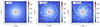 |
Fig. C.1. Time evolution of a galactic disc with a BH at rest at the centre of coordinates. The black dot indicates the BH of mass =1.25 × 10⁷ M⊙. A white dot indicates a test star which remains on a steady orbit. The time runs from left to right as indicated. Notice how an over-density in the shape of a ring develops early on but is then wiped out by differential rotation. After ≃1 Gyr of integration time, the BH remains close to the barycentre with a velocity of ∼7km s1 in amplitude. |
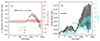 |
Fig. C.2. Time evolution of the velocity, position and angular momentum of the BH as function of time. The BH initially sits at rest at the system’s barycentre. a) The solid black curve graphs the angular momentum, which shows an irregular pattern of small amplitude; the scale’s upper bound of ≃0.5 is the value expected for a radial orbit with r = 0.125kpc at velocity vϕ = 6.6km s1 ; the right-hand axis in red is the scale for individual velocity components ; b) The radius (in black, left-hand axis) and velocity |v•| (in turquoise, right-hand axis) as function of time. The arrows indicate the spatial resolution =0.125kpc of the calculation, in black; and the expected velocity for a BH orbiting in the frozen background potential inside its influence radius, here ≃0.180kpc, in turquoise. The black dotted line is the z coordinate. Significant yet resolved motion develops only after a runtime ∼1.5 Gyr. |
The results are displayed on Figs. C.1 and C.2. On the first figure, we graph the surface density of the stars from t = 0 up to 1008 Myr of evolution, corresponding to roughly 10 orbital periods at R = 1kpc. Large-scale spiral patterns can be seen to develop and be present at all stages of evolution. The inner region runs differently, with a ring (m = 0) mode soon appearing after one period (frame t = 102 Myr) before vanishing at time t = 308 Myr and beyond. This is the expected evolution given the initial configuration. In the later stages of evolution, we find non-axisymmetric density fluctuations on a scale of ∼1kpc, but hardly any in the core region. The free motion of the BH triggers fluctuations in the potential which remain on an amplitude coherent with the numerical resolution of the calculation. For example, the BH remains confined to its radius of influence (≈180pc; see Fig. C.2[b]) and essentially bound by the numerical resolution, indicated with a black arrow on the figure. For reference, we give the amplitude of the linear velocity of harmonic motion on a scale of the BH radius of influence as a red arrow : the residual motion of the BH which builds up over ∼1.5 Gyr of evolution is therefore in agreement with analysis and sets a reference for the interpretation of our results.
C.1. Angular momentum conservation
A crucial aspect for our study of angular momentum transfer is the conservation of angular momentum by the stars, and by the BH itself. The time evolution of the BH’s angular momentum and velocity vector are displayed on Fig. C.2(a). The z-component of the angular momentum is shown in black (left-hand vertical axis). It appears to evolve somewhat stochastically, and crucially begins to change sign after t = 750 Myr ; the same applies to the radial and azimuthal velocity components, which oscillate about 0km s1 (the statistical expectancy). Overall the total system angular momentum was conserved to a relative error of 0.1% after t = 1000 Myr of evolution, and to 0.4% after t = 1500 Myr: the numerical drift gives an important clue to what will come later when the BH is set in motion. This global behaviour is similar to Brownian motion due to the graininess of the potential (Merritt et al. 2007). This is confirmed by monitoring the (3D) radius and velocity over time (Fig. C.2[b]). We performed a second set of tests (no shown here) with the Barnes-Hut integrator replaced with the direct-summation Hermite code PH4 to ensure that the trends are not enhanced or affected by the choice of integration method. The dispersion in the results obtained with different integrators for these reference configurations are standards against which to identify a genuine physical trend in thecalculations.
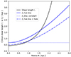 |
Fig. C.3. The figure graphs the critical length l⋆ of Eq. (D.4) as a function of the cylindrical radius, R. The Jeans lengths λJ are shown in blue. The dotted line has λJ= constant, the central value. The solid blue line recomputes the Jeans length using the local density ρ(R, 0). The dot-dash blue line is the situation when both the disc and halo are live components. Notice how l⋆ ≈ λJ around the origin. When l⋆ < λJ, the differential rotation contributes to erode a fragmentation mode. |
Appendix D: Stability analysis
We are interested in the stability of the stellar disc before a perturbation (the BH) is introduced. Details of the calculations and definitions can be found in Binney & Tremaine (2008).
D.1. Jeans modes, Toomre’s Q
The scale at which self-gravity becomes significant is given by the Jeans length,
 (D.1)
(D.1)
where σ⋆ is the three-dimensional stellar velocity dispersion, and ρ0 the central density. We compute for σ⋆ ≃ 7.3km s1 a length λJ ≈ 478pc from (D.1), significantly larger than the vertical scale height b = 250pc used for the initial configuration. Therefore, we do not expect significant evolution of the vertical disc structure.
A stellar distribution is stable (in a local sense) against all axisymmetric radial modes of fragmentation when (see §6.2 of Binney & Tremaine 2008)
 (D.2)
(D.2)
This Toomre (1964) Q parameter combines the radial epicyclic frequency κ, surface density Σ as well as the radial velocity dispersion, σR. The epicyclic frequency is easily computed from (15) and (14) after summing over the potentials ((see Binney & Tremaine 2008, Eqs. 3.79)). This leads to a mean value

with a trend of decreasing Q with increasing radius ; in fact, Q peaks at Q ≃ 1.2 near the origin, and comes down to Q ≈ 0.45 when R = 5kpc. Therefore we expect over-dense patterns to form more easily outside the region R = a while no or only a few Jeans-type fragments should develop in the nearly harmonic core. We recall that Q ≃ 1 is a threshold value, and hence the self-gravity of large fluctuations may yet develop to some degree (see Renaud et al. 2021 for a critical assessment of Q).
D.2. Differential rotation and self-gravity
The disc stars are not fully self-gravitating so the connection between velocity dispersion, angular velocity and surface density is not as in Toomre (1964)’s analysis leading to (D.2). To quantify the importance of the external potential, we compare the scale l⋆ at which differential rotation is important, to the Jeans length λJ. We fix z = 0 throughout.
Two points separated radially by a length l⋆ have a relative azimuthal velocity to first-order in l⋆/R given by
 (D.3)
(D.3)
We now focus on the situation where an over-dense clump of mass MJ forms which spawns a volume of diameter =2λJ. A star approaching MJ will not be bound to it if  , or
, or
 (D.4)
(D.4)
where we have made use of the effective frequency8
Note that the density ρ in (D.4) is that of the live (disc) component alone; and that Δ = Ω in the limit when dΩ/dR = 0 (solid body rotation). When l⋆ ≤ λJ, the shear dissolves a Jeans-unstable fragment and stabilises the disc against local collapse ; otherwise when l⋆ > λJ, the differential rotation cannot stop the Jeans fragmentation mode from growing.
The transition from one regime to the other is displayed on Fig. C.3 for the reference configuration (see §4.1). The black curve on Fig. C.3 is the solution for l⋆ from (D.4). Inspection of the figure shows that shearing takes place on a scale significantly smaller than the local Jeans length λJ= constant in the region inside radius R = 0.82kpc (dotted blue line). This holds true throughout the region R = a = 1.5kpc if we use the local value of λJ (solid blue curve; the cross-over to l⋆ > λJ occurs at R = 1.55(3)kpc).
In conclusion, we find that the Toomre criterion points to a marginally unstable core region with  on average. Because the stellar orbits are not fully self-gravitating, we argue that differential rotation helps curtail the growth of fragmentation modes in the central region: they should not form there unless triggered by a perturbation. By comparison, the tidal field of a background potential almost always contributes to slow down fragmentation modes; they have a limited impact when the density gradients are weak, which is the case in the core region ((see Binney & Tremaine 2008, §5) ; and e.g. Renaud et al. 2011 for a general tensor treatment of tidal fields). On the larger scale, however, we computed a low value Q ≈ 0.45 and so from the analysis we can anticipate the formation of large spiral features outside the core length a. This is borne out by the outcome of numerical integrations shown on Fig. C.1.
All Tables
All Figures
|
Fig. 1. Sketch of gravitational accelerations for two different situations. The panels show a massive body (blue dot) orbiting among stars, and the system’s barycentre at the bottom is the focus of the global gravitational acceleration gcm (open circle). The mean field acceleration gives rise to a velocity component δv• along the vertical y-axis. In panel (a), a massive perturber moves at some velocity v• in an isotropic field of stars; the result of the polarisation of the stellar orbits is a net dynamical friction force a∥, parallel but in the opposite sense to v•. In panel (b), the massive body is ejected from the origin at a velocity δv• pointing upwards. It orbits in a strongly anisotropic (rotating) stellar field and slows down due to the steady negative acceleration gcm. However, dynamical friction now contributes two terms, one a∥ as before, and a second one, a⊥, orthogonal to δv•. That non-zero component due to the streaming stars causes a steady transfer of angular momentum to the perturber. We refer to this second component as dynamical traction acting on the perturber. |
| In the text | |
|
Fig. 2. Rates of specific kinetic energy diffusion, ⟨ΔE⟩, as a function of the azimuthal velocity, vϕ. The rates are evaluated from Eqs. (A.7) and (A.3) for two values of the stellar velocity dispersion, σ⋆ : 20km s1 (in black or grey); and 10 km s1 (in blue or skyblue). A) Setting M• = 1 × 10⁷ M⊙, with M•/m⋆ ≃ 103, the figure graphs each quadratic component and the first-order parallel one (v∥ ⟨Δv∥⟩, dark solid lines; we note that it has the same sign as RΩ − vϕ). B) The same but for a BH with M• = 1 × 10⁸ M⊙ (M•/mstar ≃ 104). The much higher inertia of the BH leads to a ten-fold increase in the parallel term but only subtle differences in the diffusion (quadratic) ones. The light and dotted-blue curves peak off scale in either case. The (central) angular velocity Ω = 0.05/Myr is such that RΩ ≈ 70km s1 at R = 1.5kpc, a good match to the circular velocity at that radius. |
| In the text | |
|
Fig. 3. Amplitude of the BH velocity components as a function of time. The figure graphs the velocity dispersion for each parallel and orthogonal component (denoted as σ∥ or ⊥ in the legend) and the (first-order integrated) streaming velocity (v∥, black solid line). The period of a circular orbit at radius R = 1kpc (1.5kpc) is ≃61 Myr (95 Myr). |
| In the text | |
|
Fig. 4. Critical line of stability for various configurations. The vertical axis is the BH mass M• plotted against azimuthal velocity vϕ. At fixed M•, the minimum azimuthal velocity vϕ to reach such that the dynamical traction sets in is found by crossing one of the black curves, from left, to right. Four curves are plotted, each corresponding to a different value of the stellar velocity dispersion σ⋆ as indicated in the legend. The blue dot marks the estimated coordinates of the Milky Way’s BH. The red curve highlights an asymptotic trend of slop ≃ − 2 found in the limit of low vϕ. |
| In the text | |
|
Fig. 5. Case when a BH is let go from R = 1.5kpc in a (dynamically) warm stellar disc (Table 1). In panel (a), the run of Lz is shown as a black solid curve, and radial and azimuthal velocity components are shown in red. In panel (b), the cylindrical radius R and the amplitude of v• are displayed, each with their own colour-coded vertical axis. In the early stage, dynamical friction makes the orbit shrink; however, the perturber BH acquires angular momentum throughout (panel [a], black curve). Both R and v• increase systematically from t ≈ 500 Myr onward. The dotted line at the bottom is the z-coordinate bound to ±15pc. Compare with the test case displayed on Fig. C.2. |
| In the text | |
|
Fig. 6. Similar to Fig. 5 but now the BH started at R = 1.5kpc on a circular orbit. We note the sharp response of the axi-symmetric disc to the BH, which triggers radial motion. The disc adjusts to the black hole perturbation and settles progressively over several orbital times to a new equilibrium. The BH’s orbit, however, does not migrate significantly over the full integration time. Panel (a): Run of Lz (black solid curve). Radial and azimuthal velocity components are shown in red. Panel (b): Cylindrical radius R (in black) and amplitude of v• (in turquoise). The dotted line at the bottom is the z-coordinate bound to ±17pc. |
| In the text | |
|
Fig. 7. Evolution of the system when the BH is released from rest at a radius of r = 1.5kpc (from top left to bottom right). The black arrow indicates the velocity vector. Large density fluctuations soon develop in the inner ∼1kpc where the BH potential becomes dominant. After t ≈ 100 Myr of evolution, strong density fluctuations appear, including large-scale voids (deep blue). The BH used in the calculation had a mass M• = 1.25 × 10⁷ M⊙. |
| In the text | |
|
Fig. 8. Transition to a fragmented morphology for a galactic disc perturbed by a massive BH. Left-hand panels: Density map of stars with peaks indicated in red. Right-hand panels: Velocity field. A black dot indicates the BH of 1.25 × 10⁷ M⊙ (or, ≃1% the mass of the stars), with its velocity vector also in black. The configurations are displayed at three different times: 144 (top), 308 (middle), and 452 Myr (bottom row) of evolution. Contour levels in yellow (left-hand panel) and grey (right-hand panel) identify the member stars of the clump formed at t = 452 Myr. The BH sits at ≃52pc of the coordinates centre. The relative velocity between the clump’s centre of mass motion and the BH is indicated with an arrow on both panels, pointing in a north, north-west direction (west is to the left). |
| In the text | |
|
Fig. 9. Case of a BH falling from rest on a radial orbit. a) The solid black curve graphs the angular momentum accrued over time (left-hand axis with black labels); the right-hand axis is the scale for each velocity component (red curves). b) The cylindrical radius (in black, left-hand axis) and velocity (right-hand axis, in turquoise) are shown as a function of time. The dotted line at the bottom is the z coordinate bound to ±12pc. |
| In the text | |
|
Fig. 10. Similar to Fig. 9 but for when the BH is launched from the origin at vy = 80km s1 and comes to rest at a radius of R ≃ 1.35kpc. The run of all quantities are remarkably similar, but for a shift in time of ≈200 Myr (≈ two orbital times) when Lz peaks. We also note that the phase of dynamical friction does not bring the BH close to the origin, as its apocentre distance always exceeds 250pc. The gain in angular momentum seen in panel (a; black curve) begins before 500 Myr. |
| In the text | |
|
Fig. 11. Evolution of the BH set on a circular orbit initially of radius r = 1.5kpc (top left to bottom right). The black arrow indicates the velocity vector. Large spiral waves and Jeans fragments develop quickly due to the lower stellar velocity dispersion. The BH binds with stars and opens a gap in its wake, which leads to a steady loss of angular momentum and inward migration. This is most visible in the frames with time running from t = 41 Myr to 915 Myr. At t = 915 Myr the BH sits at r ≈ 20pc with a rest-frame velocity ≃9km s1. Non-axi-symmetric clumps of stars dislodge the BH which acquires significant angular momentum by dynamical traction in the later stages of evolution (on a timescale ∼500 Myr). Calculations performed with a BH of mass M• = 1.25 × 10⁷ M⊙. |
| In the text | |
|
Fig. 12. Runs of angular momentum, radius, and velocity components as a function of time for a BH started on a circular orbit. a) The solid black curve graphs the angular momentum (left-hand axis with black labels). The right-hand axis is the scale for each velocity component (red curves). b) The cylindrical radius (in black, left-hand axis) is graphed together with the norm of the velocity (right-hand axis, in turquoise). The dotted line at the bottom is the z coordinate bound to ±10pc. The radius and velocity components reach a minimum at t = 915 Myr. |
| In the text | |
|
Fig. 13. Runs of angular momentum and radius for three BH orbits: circular; an elliptical orbit with a small eccentricity, e ≈ 0.55; and a third case with a large eccentricity, e ≈ 0.67. a) Run of the angular momentum for each case as indicated in the legend. The solid black curve graphs Lz for the circular initial orbit displayed on Fig. 12. b) Cylindrical radius as a function of time for the same three cases. We note how the BH orbit with the more elliptical orbit actually evolves at a near-constant mean radius. |
| In the text | |
|
Fig. 14. A) Specific angular momentum, Lz, as a function of the cylindrical radius, R, during the orbital migration of the BH. The large sky-blue arrows indicate the flow of time, t. The orange solid lines trace the expected values for the model galaxy. The curve in blue (red) shows the coordinates before (after) Lz has reached a maximum. The black lines indicate evolution at a constant Lz. The circles numbered 1 and 2 single out specific phases of evolution. B) Run of azimuthal velocity, vϕ, against radius, R. The axes have been shifted for clarity. The colour-coding for the other curves and symbols is as for (A). |
| In the text | |
|
Fig. 15. Two examples of the interaction between the central BH and stellar sub-structures. In (A, top row), when the background spherical Isochrone potential is partially frozen, the disc stars form clumps of higher mass and binding energy. Such structures may dislodge the BH. This two-stage instability then grows as the BH extracts angular momentum from the flow of rotating stars around the centre. In (B, bottom row) the situation for a self-gravitating disc plus isochrone potential means that the clumps are much less massive and of a lower binding energy. In that case, a clump will dissolve in the strong tidal field of the BH. The centre of coordinates is indicated with a red dot. (See text for more details). |
| In the text | |
|
Fig. C.1. Time evolution of a galactic disc with a BH at rest at the centre of coordinates. The black dot indicates the BH of mass =1.25 × 10⁷ M⊙. A white dot indicates a test star which remains on a steady orbit. The time runs from left to right as indicated. Notice how an over-density in the shape of a ring develops early on but is then wiped out by differential rotation. After ≃1 Gyr of integration time, the BH remains close to the barycentre with a velocity of ∼7km s1 in amplitude. |
| In the text | |
|
Fig. C.2. Time evolution of the velocity, position and angular momentum of the BH as function of time. The BH initially sits at rest at the system’s barycentre. a) The solid black curve graphs the angular momentum, which shows an irregular pattern of small amplitude; the scale’s upper bound of ≃0.5 is the value expected for a radial orbit with r = 0.125kpc at velocity vϕ = 6.6km s1 ; the right-hand axis in red is the scale for individual velocity components ; b) The radius (in black, left-hand axis) and velocity |v•| (in turquoise, right-hand axis) as function of time. The arrows indicate the spatial resolution =0.125kpc of the calculation, in black; and the expected velocity for a BH orbiting in the frozen background potential inside its influence radius, here ≃0.180kpc, in turquoise. The black dotted line is the z coordinate. Significant yet resolved motion develops only after a runtime ∼1.5 Gyr. |
| In the text | |
|
Fig. C.3. The figure graphs the critical length l⋆ of Eq. (D.4) as a function of the cylindrical radius, R. The Jeans lengths λJ are shown in blue. The dotted line has λJ= constant, the central value. The solid blue line recomputes the Jeans length using the local density ρ(R, 0). The dot-dash blue line is the situation when both the disc and halo are live components. Notice how l⋆ ≈ λJ around the origin. When l⋆ < λJ, the differential rotation contributes to erode a fragmentation mode. |
| In the text | |
Current usage metrics show cumulative count of Article Views (full-text article views including HTML views, PDF and ePub downloads, according to the available data) and Abstracts Views on Vision4Press platform.
Data correspond to usage on the plateform after 2015. The current usage metrics is available 48-96 hours after online publication and is updated daily on week days.
Initial download of the metrics may take a while.