| Issue |
A&A
Volume 701, September 2025
|
|
|---|---|---|
| Article Number | A150 | |
| Number of page(s) | 27 | |
| Section | Numerical methods and codes | |
| DOI | https://doi.org/10.1051/0004-6361/202554025 | |
| Published online | 12 September 2025 | |
Learning novel representations of variable sources from multi-modal Gaia data via autoencoders
1
Institute of Astronomy, KU Leuven,
Celestijnenlaan 200D,
3001
Leuven,
Belgium
2
Millennium Institute of Astrophysics,
Nuncio Monseñor Sotero Sanz 100, Of. 104, Providencia,
Santiago,
Chile
3
Department of Astronomy, University of Geneva,
Chemin Pegasi 51,
1290
Versoix,
Switzerland
4
Department of Astronomy, University of Geneva,
Chemin d’Ecogia 16,
1290
Versoix,
Switzerland
5
Sednai Sàrl,
Geneva,
Switzerland
6
INAF – Osservatorio Astrofisico di Torino,
Via Osservatorio 20,
10025
Pino Torinese,
Italy
7
Konkoly Observatory, HUN-REN Research Centre for Astronomy and Earth Sciences,
Konkoly Thege 15–17,
1121
Budapest,
Hungary
8
CSFK, MTA Centre of Excellence,
Konkoly Thege 15–17,
1121
Budapest,
Hungary
9
INAF – Osservatorio di Astrofisica e Scienza dello Spazio di Bologna,
Via Piero Gobetti 93/3,
Bologna
40129,
Italy
10
Starion for European Space Agency, Camino bajo del Castillo, s/n, Urbanizacion Villafranca del Castillo, Villanueva de la Cañada,
28692
Madrid,
Spain
11
Department of Astrophysics, IMAPP, Radboud University Nijmegen,
PO Box 9010,
6500
GL
Nijmegen,
The Netherlands
12
Max Planck Institute for Astronomy,
Koenigstuhl 17,
69117
Heidelberg,
Germany
★ Corresponding author: This email address is being protected from spambots. You need JavaScript enabled to view it.
Received:
4
February
2025
Accepted:
18
July
2025
Abstract
Context. Gaia Data Release 3 (DR3) has published for the first time epoch photometry, BP/RP (XP) low-resolution mean spectra, and supervised classification results for millions of variable sources. This extensive dataset offers a unique opportunity to study the variability of these objects by combining multiple Gaia data products.
Aims. In preparation for DR4, we propose and evaluate a machine learning methodology capable of ingesting multiple Gaia data products to achieve an unsupervised classification of stellar and quasar variability.
Methods. A dataset of 4 million Gaia DR3 sources was used to train three variational autoencoders (VAEs), which are artificial neural networks (ANNs) designed for data compression and generation. One VAE was trained on Gaia XP low-resolution spectra, another on a novel approach based on the distribution of magnitude differences in the Gaia G band, and the third on folded Gaia G band light curves. Each Gaia source was compressed into 15 numbers, representing the coordinates in a 15-dimensional latent space generated by combining the outputs of these three models.
Results. The learned latent representation produced by the ANN effectively distinguishes between the main variability classes present in Gaia DR3, as demonstrated through both supervised and unsupervised classification analysis of the latent space. The results highlight a strong synergy between light curves and low-resolution spectral data, emphasising the benefits of combining the different Gaia data products. A 2D projection of the latent variables revealed numerous overdensities, most of which strongly correlate with astrophysical properties, showing the potential of this latent space for astrophysical discovery.
Conclusions. We show that the properties of our novel latent representation make it highly valuable for variability analysis tasks, including classification, clustering, and outlier detection.
Key words: methods: data analysis / methods: numerical / methods: statistical / techniques: photometric / techniques: spectroscopic / stars: variables: general
© The Authors 2025
 Open Access article, published by EDP Sciences, under the terms of the Creative Commons Attribution License (https://creativecommons.org/licenses/by/4.0), which permits unrestricted use, distribution, and reproduction in any medium, provided the original work is properly cited.
This article is published in open access under the Subscribe to Open model. This email address is being protected from spambots. You need JavaScript enabled to view it. to support open access publication.
1 Introduction
Since its launch in 2013, the European Space Agency’s Gaia mission (Gaia Collaboration 2016) has been surveying more than a billion astronomical sources, charting their positions, luminosities, temperatures, and compositions. The Gaia Data Release 3 (DR3) catalogue (Gaia Collaboration 2023b), published in June 2022, marks a significant milestone in the mission, providing the results of 34 months of observations processed by the Gaia Data Processing and Analysis Consortium (DPAC). Gaia DR3 also represents a substantial improvement over previous data releases, offering an increase not only in the quantity and quality of the data but also in the variety of data products available for the community.
Gaia DR3 has been particularly relevant for variability analysis (Eyer et al. 2023), as it offers photometric time series in three bands for 11.7 million sources and low-resolution spectra (Carrasco et al. 2021; De Angeli et al. 2023) for more than 200 million sources. In addition, the variability processing and analysis coordination unit at the Gaia DPAC (DPAC-CU7) classified variable sources into 25 classes using supervised machine learning (ML) techniques (Rimoldini et al. 2023). The published variability classifications for DR3 were generated by combining the outputs of several ML models trained with two supervised ML algorithms: random forest (Breiman 2001) and XGBoost (Chen & Guestrin 2016). These classifiers based their predictions on approximately 30 attributes (features) derived from Gaia’s astrometry and epoch photometry data, mainly time series statistics, periodicity indicators, and colour information. The models were trained on a subset of Gaia sources with known ground truth variability classes selected from the crossmatch of 152 catalogues from the literature (Gavras et al. 2023).
Although a supervised classification of sources into a set of predefined classes is a crucial prerequisite for follow-up astrophysical analysis, it does not allow for the discovery of new groups or subgroups of variable sources. Such (sub)groups may have remained unnoticed before because the relevant parameter space was too sparsely populated to note them, but they may now be visible with the huge number of sources that Gaia is observing. Finding an over- or underdensity in a parameter space is, however, computationally daunting. On the one hand, the sheer size of the Gaia archive implies that any discovery method must be able to cope with hundreds of millions of sources. On the other hand, Gaia provides a large diversity of data products, which also make the parameter space high dimensional.
In preparation for Data Release 4 (DR4), with this work we present an unsupervised ML method that combines multiple Gaia products in a novel way. Unlike supervised methods, it does not require predefined variability classes nor does it rely on classification labels available in the literature, thereby avoiding potential biases arising from the selection and availability of training labels. By not imposing a predefined set of categories, unsupervised methods are particularly well suited to objective data exploration and hunting for novelties or anomalies. However, as we show, this flexibility also introduces significant challenges in evaluation and interpretation compared to supervised approaches.
A second important feature of our method is that it is able to exploit multiple Gaia data products as input, namely, the epoch photometry and the low-resolution BP/RP (XP) mean spectra. These data products (sometimes referred to as ‘modalities’) are fed to artificial neural networks (ANNs) to generate a compressed set of features. This falls within the field of self-supervised representation learning (SSRL; e.g. Bengio et al. 2013; Gui et al. 2024; Donoso-Oliva et al. 2023), which describes a collection of ANN-based methodologies used to discover numerical representations from complex data in order to facilitate downstream tasks, such as classification, clustering, and anomaly detection. Like traditional unsupervised methods, SSRL techniques do not rely on manually annotated labels. Instead, they generate supervisory signals directly from the input data. Two prominent SSRL approaches are autoencoders (AEs; e.g. Naul et al. 2018; Jamal & Bloom 2020) and contrastive learning (CL; e.g. Liu et al. 2021; Huertas-Company et al. 2023). In particular, AEs learn representations by compressing the data and then minimising the error between the original and an approximation reconstructed from its compressed version. These representations are referred to as latent variables, as they encapsulate the underlying features that summarise the observed variables. Multimodal SSRL (Guo et al. 2019; Radford et al. 2021) involves training AE or CL models from examples that span multiple modalities, often captured by different sensors. In astronomy, for instance, different modalities may consist of photometric and spectroscopic data (The Multimodal Universe Collaboration 2024). Here, we explore the synergies between Gaia DR3 epoch photometry and XP mean spectra in the context of variability analysis.
We expect the results presented here to serve as a proof of concept for a future implementation using Gaia DR4, which is scheduled for publication in 2026. DR4 will double the number of measurements compared to previous data releases, and more importantly, it will provide epoch photometry for all observed sources rather than just those classified as variables in DR3. Additionally, DR4 will include new data products, such as time series data for XP spectra, among others1. The ML models capable of exploiting these rich data products will be essential for the automatic analysis of variable sources.
This article is organised as follows: in Section 2, we place our method in the context of related work in the literature. In Section 3, we describe the datasets used to train the proposed models. In Section 4, we detail the theoretical foundations and implementation details of the models for each data modality. In Section 5, we explain how the dimensionality of the latent variable vector is set. The quality of our learned representation is evaluated through outlier detection, classification, and clustering tasks, and the results are presented in Sections 6, 7, and 8, respectively. Section 9 provides an astrophysical interpretation of the learned representations. Finally, our conclusions are summarised in Section 10.
2 State-of-the-art of representation learning
Autoencoders have previously been proposed to analyse Gaia data products. Laroche & Speagle (2023) introduced a variational autoencoder (VAE; Kingma & Welling 2014) that takes normalised XP mean spectra coefficients as input and compresses them into six latent variables. The authors demonstrated that these latent variables can predict stellar parameters, such as effective temperature (Teff), surface gravity, and iron abundance ([Fe/H]), with greater accuracy than a purely supervised model. This highlights the benefits of leveraging large quantities of unlabelled data. Martínez-Palomera et al. (2022) trained a VAE to generate light curves of periodic variable stars using cross-matched data from OGLE-III (Udalski et al. 2008) and Gaia DR2. Specifically, the model was trained to reconstruct OGLE’s folded light curves conditioned on Gaia’s physical parameters, e.g. Teff, stellar radius and luminosity. They achieved this by training a regressor that predicts the VAE’s latent variables from the physical parameters, obtaining a physically enhanced AE that acts as an efficient variable star simulator. In our work, the main focus is on the self-supervised learning of the latent variables, rather than on the data generation aspects of VAE, although the latter are used to help interpret the results.
Multimodal learning leveraging multiple Gaia data products has also been explored in previous studies. Guiglion et al. (2024) proposed a supervised ANN to predict stellar parameters and chemical abundances by combining Gaia Radial Velocity Spectrometer (RVS) spectra (Sartoretti et al. 2023), XP mean spectra, mean photometric magnitudes, and parallaxes. Their dataset included 841 300 Gaia DR3 sources, of which 44780 had stellar labels derived from APOGEE DR17 (Abdurro’uf et al. 2022). Training the model on these combined modalities enabled the authors to resolve and trace the [α/M]–[M/H] bimodality in the Milky Way for the first time, demonstrating the power of integrating diverse data sources. Using the same dataset and similar architectures, Buck & Schwarz (2024) applied CL to train an ANN capable of projecting RVS and XP spectra into a shared latent space. They showed that the resulting latent space is highly structured and achieved good performance in both spectra generation and stellar label prediction. Here, we choose to combine XP mean spectra with epoch photometry data and exclude mean RVS spectra, as the latter are only available for bright sources and have a small intersection with public epoch photometry data.
Other recent examples of large ANN models trained using multimodal astronomical data include Parker et al. (2024); Zhang et al. (2024); Rizhko & Bloom (2025). These studies leverage Contrastive Language-Image Pre-Training (CLIP; Radford et al. 2021), a technique where different modalities are projected into latent vectors using ANNs and aligned by minimising their distance in the latent space. Parker et al. (2024) focused on extragalactic objects, training their model on 197 632 pairs of optical spectra and images from DESI (DESI Collaboration 2024). In contrast, Zhang et al. (2024) focused on supernovae and proposed a model that takes multiband difference photometry and spectra as input. The model was initially trained on 500 000 simulated events and subsequently fine-tuned using 4702 data pairs from the ZTF (Bellm et al. 2019) and the Spectral Energy Distribution Machine (Blagorodnova et al. 2018). Although extragalactic sources are also considered in this work, our focus is on general variability classification applied to Gaia DR3 public data, which includes multiple classes of variable stars.
In this context, the study by Rizhko & Bloom (2025) is more closely related to ours, as it considered ten stellar variability classes, including subtypes of eclipsing binaries, RR Lyrae and δ Scuti stars. Their model was trained on 21 708 sources, integrating light curves from the ASAS-SN variable star catalogue (Jayasinghe et al. 2019), spectra from the LAMOST (Cui et al. 2012), and additional features such as galactic coordinates, magnitudes from multiple surveys and parallaxes from Gaia EDR3. The models for each modality are jointly trained using CLIP and then fine-tuned to solve a classification task. Fine-tuning refers to the process of adapting a pre-trained model to a new task by continuing training on labelled data. The results achieved by Rizhko & Bloom (2025) show that self-supervised pre-training is beneficial in scenarios with limited labelled data and that the resulting latent space is useful not only for classification but also for outlier detection and similarity searches.
In this work, we propose an AE-based model that generates a latent space where variability classes are well organised without relying on simulated data or fine-tuning via labels. The model is trained using more than 4 million sources with Gaia DR3 epoch photometry and low-resolution spectral data covering a wide range of variable phenomena. We leave the inclusion of additional data products, such as Gaia astrometric information or data from other surveys, for future work.
3 Datasets
3.1 Training data
To construct the dataset used to train the ANN, we started from the 11 754 237 Gaia DR3 sources that have publicly available epoch photometry data. This dataset comprises 10 509 536 sources identified as variable (Eyer et al. 2023) and another 1 244 319 sources with time series from the Gaia Andromeda Photometric Survey (Evans et al. 2023). We further filtered this set by requiring the sources to have XP mean spectra coefficients available (De Angeli et al. 2023). This filtering step removed 5 381 570 sources, predominantly faint ones, with 82.2% and 21.3% having a G band median magnitude above 18 and 20, respectively. Finally, we excluded sources with fewer than 40 observations (sparser time series yield less reliable results), yielding a total of 4 136 544 sources for training and evaluating the proposed models. This limit in data points follows Gaia Collaboration (2023a) and ensures the reliability of the learned representations. Only 60 295 sources have RVS spectra available within the dataset. Appendix A provides the ADQL query to retrieve the source identifiers (ids) of the training set.
Using the source ids, we obtained light curves and XP mean spectra through the Gaia datalink service via the interface provided by the astroquery Python package (Ginsburg et al. 2019). Gaia DR3 provides epoch photometry data in the form of G, GBP, and GRP light curves, which are obtained from the DR3 epoch_photometry table as a collection of arrays. Observation times and magnitudes for the G band were extracted from the g_transit_time and g_transit_mag arrays, respectively. Magnitude uncertainties are not provided but can be estimated using the g_transit_flux_over_error array. Observations flagged as spurious or doubtful by DPAC-CU7 were removed from the light curves by applying the variability_flag_g_reject2 array.
Gaia’s blue (BP) and red (RP) onboard spectrophotometers enable the collection of low-resolution epoch spectra. Carrasco et al. (2021) details the process by which these data are internally calibrated and time-averaged to produce the XP mean spectra published in Gaia DR3. These spectra are provided through the xp_continuous_mean_spectrum table as two 55-dimensional real-valued arrays per source, bp_coefficients and rp_coefficients, representing the coefficients of a Hermite-polynomial basis for BP and RP, respectively. This continuous representation can be converted into an internally calibrated flux versus pseudo-wavelength format using the GaiaXPy Python package (Ruz-Mieres 2024), which is the format used in this work.
3.2 Data used for evaluation purposes
A subset of 38 740 sources within the training set have reliable variability class information. This subset corresponds to a selection from the cross-match by Gavras et al. (2023) after applying the procedures described in Section 3.1.2 and Appendix A of Rimoldini et al. (2023). We refer to this as the labelled subset. The light curves and mean spectra of these sources are also part of the training dataset. However, the proposed models are not trained using their class labels. Instead, the variability class labels are solely used to evaluate how well the learned representations distinguish between different variability classes.
For this evaluation, we adopted a taxonomy comprising 22 classes, including
Cepheids divided into 1052 δ Cepheids (δ Cep) and 538 type-II Cepheids (t2 Cep). These are radially pulsating variables with periods ranging from approximately 1 day to hundreds of days.
RR Lyrae (RR Lyr) stars divided into 1875 type-ab (RR Lyr ab), 1313 type-c (RR Lyr c), and 696 type-d (RR Lyr d) pulsators. These are pulsating variables whose dominant radial modes have periods between 0.2 and 1 day.
Eclipsing binary stars (ECL) divided into 1736 Algol-type (ECLa), 2672 β Lyrae-type (ECLb), and 1890 W Ursae Majoris-type (ECLw).
Long period variables (LPVs), including Mira variables and various semiregular variables, with 10 751 sources in total.
Other pulsating variables including 111 β Cephei (β Cep) stars, 4372 δ Scuti (δ Sct) stars, 381 γ Doradus (γ Dor) stars, 93 slowly pulsating B (SPB) stars, and 149 pulsating white dwarfs (WDs).
Rotational variables including 946 RS Canum Venaticorum stars (RSs), 248 ellipsoidal variables (ELLs), and 5164 generic solar-like variables (SOLAR). Following Rimoldini et al. (2023), we also consider a merged class (ACV|CP) with 979 sources, that combines α2 Canum Venaticorum, magnetic chemically peculiars, and generic chemically peculiar (CP) stars.
Eruptive variables including 1699 young stellar objects (YSOs). Following Rimoldini et al. (2023), we also consider a merged class (BE|GCAS) that combines B-type emission line variables and γ Cassiopeiae stars with 752 sources in total.
Cataclysmic variables (CVs) of various types with 256 sources in total.
Active galactic nuclei (AGNs) of different types, with 1067 sources in total.
We refer the reader to Gavras et al. (2023) for a more detailed description of each of the classes.
We also considered the classifications published in the Gaia DR3 vari_classifier_result table to evaluate the learned representations. These labels are the result of the general variability classification carried out by Rimoldini et al. (2023). A total of 3 738 644 sources in our training dataset have this information available. Gaia DR3 also published the results of several specific object study (SOS) pipelines. In this case, we retrieved information from the vari_rrlyrae, vari_eclipsing_binary, vari_long_period_variable and vari_agn tables, which contain features extracted by Clementini et al. (2023), Mowlavi et al. (2023), Lebzelter et al. (2023) and Carnerero et al. (2023), respectively. The training set includes 48 753 sources from the RR Lyr stars SOS table, 486 871 from the eclipsing binaries SOS table, 513 208 from the LPVs SOS table, and 51 714 from the AGNs SOS table.
4 ANN architecture
Undercomplete AEs are a type of ANN designed to compress complex data into a more compact form (Goodfellow et al. 2016). They consist of two main components: an encoder, which extracts a compact set of latent variables from the input data, and a decoder, which reconstructs the input data from these latent variables. Compression is achieved by limiting the number of latent variables, that is, the dimensionality of the latent space, to be much smaller than that of the input data while minimising the difference between the input and output of the AE:
![Mathematical equation: $\[\theta^*, \phi^*=\min _{\theta, \phi} \sum_{i=1}^N L\left(\boldsymbol{x}_i, \theta, \phi\right)\]$](/articles/aa/full_html/2025/09/aa54025-25/aa54025-25-eq1.png) (1)
(1)
![Mathematical equation: $\[=\min _{\theta, \phi} \sum_{i=1}^N\left\|\boldsymbol{x}_i-\operatorname{Dec}_\theta\left(\operatorname{Enc}_\phi\left(\boldsymbol{x}_i\right)\right)\right\|^2,\]$](/articles/aa/full_html/2025/09/aa54025-25/aa54025-25-eq2.png) (2)
(2)
where {xi}i=1,...,N with xi ∈ ℝD is the training dataset and L(·, ·, ·) is the cost function that measures the error between the input and its reconstruction, the most widely used being the mean square error, in Eq. (2). The encoder and the decoder are non-linear maps Encϕ: ℝD → ℝK and Decθ: ℝK → ℝD, with trainable parameters denoted by ϕ and θ, respectively, and K ≪ D is the latent space dimensionality. Once the optimal parameters ϕ*, θ* are determined, the encoder can be used to obtain the latent variables for a given input as zi = Encϕ* (xi).
The VAE (Kingma & Welling 2014) differs from conventional AEs by giving a probabilistic interpretation to the decoder and encoder output. Specifically, the decoder is modelled as a generative process described by the conditional distribution pθ(x|z), parametrised by θ, while the encoder is represented by the conditional distribution qϕ(z|x), parametrised by ϕ. The encoder serves as a variational approximation of the intractable true posterior p(z|x) and is assumed to follow a Gaussian distribution with diagonal covariance (mean field assumption). In practical terms, this means that the encoder maps the input data to two outputs μi and ![Mathematical equation: $\[\boldsymbol{\sigma}_{i}^{2}=\operatorname{Enc}_{\phi}\left(\boldsymbol{x}_{i}\right)\]$](/articles/aa/full_html/2025/09/aa54025-25/aa54025-25-eq3.png) , corresponding to the mean and variance of the latent variables.
, corresponding to the mean and variance of the latent variables.
The VAE is trained by maximising the evidence lower bound (ELBO), defined as
![Mathematical equation: $\[L\left(\boldsymbol{x}_i, \theta, \phi\right)=\mathbb{E}_{z_i \sim q_\phi\left(z \mid x_i\right)}\left[\log~ p_\theta\left(x{ \mid} z_i\right)\right]-\beta \cdot D_{\mathrm{KL}}~[q_\phi\left(z \mid x_i) \| p(z)\right],\]$](/articles/aa/full_html/2025/09/aa54025-25/aa54025-25-eq4.png) (3)
(3)
where
![Mathematical equation: $\[D_{\mathrm{KL}}\left[q_\phi~(z {\mid} x_i) \| p(z)\right]=\frac{1}{2} \sum_{k=1}^K \mu_{i k}^2+\sigma_{i k}^2-1-\log~ \sigma_{i k}^2,\]$](/articles/aa/full_html/2025/09/aa54025-25/aa54025-25-eq5.png) (4)
(4)
is the Kullback-Leibler (KL) divergence between the encoder distribution and a standard normal prior p(z) = 𝒩(0, I). The first term in Eq. (3) is the expected value of the log-likelihood of the decoder, and to compute it, one first needs to sample the latent variables using
![Mathematical equation: $\[z_i=\boldsymbol{\mu}_i+\boldsymbol{\sigma}_i \cdot \epsilon, \quad \epsilon \sim \mathcal{N}(0, I).\]$](/articles/aa/full_html/2025/09/aa54025-25/aa54025-25-eq6.png) (5)
(5)
Maximising the likelihood increases the fidelity of the decoder reconstruction with respect to the original input and can be seen as equivalent to minimising the reconstruction error. On the other hand, minimising the KL divergence provides regularisation to the latent variables. The hyperparameter β was introduced in Burgess et al. (2018) to control the trade-off between reconstruction fidelity and latent space regularisation. It prevents over-regularised solutions where the first term of Eq. (3) is neglected. Since most optimisers are designed for minimisation, the negative ELBO is typically used in practice.
The distribution of pθ(x|z), on the other hand, is selected based on the characteristics of the data. In the following sections, we detail the preprocessing, ANN design and the choice of log-likelihood for each of the modalities considered. This includes a VAE for the XP mean spectra and two VAEs for different representations of the G band light curve.
4.1 VAE for XP mean spectra
Before entering the model, the 55 BP and 55 RP mean spectrum fluxes obtained using GaiaXPy, along with their associated uncertainties, are concatenated into two 110-dimensional vectors, x and e. Both vectors are normalised by dividing each element by the standard deviation of x. This normalisation preserves the relative differences between the BP and RP spectra while eliminating the influence of the source’s brightness. The first row in Fig. 1 shows the preprocessed XP mean spectra and corresponding VAE reconstructions of three variable sources. The third column in the plot, which corresponds to an LPV, exhibits a considerably stronger RP with respect to the other two sources. Examples for other variability classes can be found in Figs. A.1–A.4.
After preprocessing, the data is then compressed and reconstructed using a VAE with an architecture based on fully connected (FC) layers that is showcased in Fig. 2. Three layers are used for the encoder and decoder networks, respectively. Intermediate layers have 128 neurons with Gaussian error linear unit (GELU) activation functions (Hendrycks & Gimpel 2016) and layer normalisation (LN; Lei Ba et al. 2016) to enhance stability during training. The output layer of the encoder, i.e. the mean and standard deviation of the latent variables, do not incorporate LN and use a linear activation (LIN) to avoid constraining their range. The output layer of the decoder, i.e. the reconstructed mean spectra, uses the Rectified linear unit (ReLU) max(X, 0) activation (Nair & Hinton 2010; Glorot et al. 2011) to ensure non-negativity. A separate two-layer decoder network is used to predict log ![Mathematical equation: $\[\sigma_{\text {XP }}^{2}\]$](/articles/aa/full_html/2025/09/aa54025-25/aa54025-25-eq7.png) , an uncertainty term representing the logarithm of the variance of the reconstructed mean spectra. The particular choice for the number of neurons and activation functions of this network is detailed in Appendix B.
, an uncertainty term representing the logarithm of the variance of the reconstructed mean spectra. The particular choice for the number of neurons and activation functions of this network is detailed in Appendix B.
This VAE is optimised using Eq. (3) and the following Gaussian log-likelihood for a given source
![Mathematical equation: $\[\log~ p_\theta(x {\mid} z)=-\frac{1}{2}\left[\log \left(\sum_{j=1}^{110}\left(e_j^2+\sigma_{\mathrm{XP}}^2\right)\right)+\sum_{j=1}^{110} \frac{\left(x_j-\hat{x}_j\right)^2}{e_j^2+\sigma_{\mathrm{XP}}^2}\right],\]$](/articles/aa/full_html/2025/09/aa54025-25/aa54025-25-eq8.png) (6)
(6)
where ![Mathematical equation: $\[\hat{x}=\operatorname{Dec}_{\theta}(z)\]$](/articles/aa/full_html/2025/09/aa54025-25/aa54025-25-eq9.png) is the reconstructed XP spectra. Terms that do not depend on the model parameters have been omitted.
is the reconstructed XP spectra. Terms that do not depend on the model parameters have been omitted.
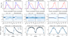 |
Fig. 1 Input data and VAE reconstructions for three variable Gaia DR3 sources. The sources shown in each column are associated with the RR Lyr ab star, ECLb, and LPV classes, respectively. Each row corresponds to a specific data modality and shows the preprocessed input data (prior to compression) and its reconstruction (after decompression) using the VAEs described in Sections 4.1, 4.2, and 4.3. The first row corresponds to the sampled representation of the Gaia BP (solid blue) and RP (dashed red) low-resolution spectra. The second row depicts the conditional distribution of magnitude differences given time differences of the Gaia G band light curves. The third row shows the Gaia G band light curve folded with its dominant period. |
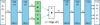 |
Fig. 2 Variational autoencoder used to create a K = 5 dimensional latent space given the 2 × 55 continuous BP and RP spectra points. Each coloured rectangle represents a layer of the ANN, with the size of the output vector given at the top. The encoder starts with the (standardised) observations denoted in the leftmost white rectangle, and ends with the K = 5-dimensional latent space denoted in green, representing the position μ and its (spherical) uncertainty σ2 of the observed data in the latent space. The decoder starts by sampling a K=5-dimensional value z from a Gaussian distribution with mean μ and the diagonal covariance matrix σ2, and ends with the reconstructed 2 × 55 XP spectra values. Some layers use ‘layer normalisation’, which is denoted by LN. The activation function of the neurons in a particular layer is noted at the bottom: GELU, LIN (linear), or ReLU. |
4.2 VAE for Δ m/Δ t of G band light curves
Variability across different time scales is a key characteristic for distinguishing between various classes of variable stars (Eyer & Mowlavi 2008). To capture this aspect, the second VAE uses a representation of the G band light curves inspired by the approaches of Mahabal et al. (2017) and Soraisam et al. (2020) as input. Specifically, we employ an estimator of the conditional distribution of magnitude changes (Δm) given time intervals (Δt), referred to here as Δm|Δt.
This distribution is estimated non-parametrically from the normalised G band light curve. A light curve, defined here as a sequence of observations (tj, mj, ej)i with j = 1, . . ., Li, where Li is the number of observations of the i-th source, is preprocessed as follows. First, observations with ![Mathematical equation: $\[e_{j}>\bar{e}+3 \sigma_{e}\]$](/articles/aa/full_html/2025/09/aa54025-25/aa54025-25-eq10.png) , where
, where ![Mathematical equation: $\[\bar{e}\]$](/articles/aa/full_html/2025/09/aa54025-25/aa54025-25-eq11.png) and σe are the mean and standard deviation of the magnitude uncertainties of the source, are removed. Then the magnitudes are centred around zero by subtracting their mean. Finally, the magnitudes and uncertainties are rescaled by dividing by the standard deviation of the magnitudes.
and σe are the mean and standard deviation of the magnitude uncertainties of the source, are removed. Then the magnitudes are centred around zero by subtracting their mean. Finally, the magnitudes and uncertainties are rescaled by dividing by the standard deviation of the magnitudes.
To compute the Δm|Δt representation, we first calculate all pairwise differences in magnitudes and observation times for a given light curve. Specifically, this involves computing the tuples (Δmj1j2 = mj2 − mj1, Δtj1j2 = tj2 − tj1), where 1 ≤ j1 < j2 ≤ Li. These tuples are then binned into a 2D histogram using the following bin definitions:
For Δt, we used five bins b(Δt): four bins defined by the following edges: 0.07, 0.1, 0.5, 20, 50 plus an extra bin for when Δt > 50. This set of bins was designed to capture astrophysically relevant timescales while ensuring that the bins are populated for all sources in the training set, thereby eliminating issues related to missing data. As a result of this design, the bins align with the typical cadences found in Gaia’s scanning law (see Gaia Collaboration 2016), focusing on observations separated by hours or months. For reference, the distribution of Δt in the 4M dataset is shown in Fig. A.5.
For Δm, we defined 23 bins b(Δm): 21 bins with linearly spaced edges between [−3, 3] plus two extra bins for Δm < −3 and Δm > 3, respectively. This set of bins was chosen to cover the range of the normalised magnitudes, with outliers being captured in the first and last bins. The normalisation procedure ensures that Δm remains centred around zero. For reference, the distribution of Δm in the 4 M dataset is shown in Fig. A.6.
This process produces a 23 × 5 sized array, representing the joint distribution of Δm and Δt. To remove the effects of time sampling and obtain the final Δm|Δt representation, the array is divided by the marginal distribution of Δt. Concretely, the value at the km-th row and kt-th column of the Δm|Δt array is given by
![Mathematical equation: $\[p_{k_m k_t}=\frac{\sum_{j_2=2}^{L_i} \sum_{j_1=1}^{j_2-1} W\left(\Delta m_{j_1 j_2}, b_{k_m}^{(\Delta m)}\right) \cdot W\left(\Delta t_{j_1 j_2}, b_{k_t}^{(\Delta t)}\right)}{\sum_{j_2=2}^{L_i} \sum_{j_1=1}^{j_2-1} W\left(\Delta t_{j_1 j_2}, b_{k_t}^{(\Delta t)}\right)},\]$](/articles/aa/full_html/2025/09/aa54025-25/aa54025-25-eq12.png) (7)
(7)
where
![Mathematical equation: $\[W(\Delta x, b)= \begin{cases}1 & \text { if } \Delta x \in b, \\ 0 & \text { otherwise}.\end{cases}\]$](/articles/aa/full_html/2025/09/aa54025-25/aa54025-25-eq13.png) (8)
(8)
The numerator in Eq. (7) counts the number of magnitude–time pairs for which the magnitude difference Δm falls into the km-th magnitude bin and the time difference Δt falls into the kt-th time bin. The denominator counts how many pairs fall into the kt-th time bin, regardless of their magnitude difference.
The middle row in Fig. 1 shows the resulting Δm|Δt representations and corresponding VAE reconstructions for three variable sources. For example, the third column, which corresponds to an LPV, exhibits near-zero difference in magnitude for time differences below 20 days. The other two sources show variability at much shorter time scales.
The Δm|Δt representation is then flattened to a 115-dimensional vector, compressed and reconstructed using a VAE with an FC architecture shown in Fig. 3 and detailed in Appendix B. This architecture is similar to the one used for the XP mean spectra but with one additional layer in the encoder and decoder networks, respectively. Additionally, a Softmax activation function is applied to the decoder output to ensure that all values are non-negative and add up to one column-wise. This VAE is optimised using Eq. (3) and the binary-cross entropy loss for a given source
![Mathematical equation: $\[\log~ p_\theta(x {\mid} z)=\sum_{k_m=1}^{23} \sum_{k_t=1}^5 p_{k_m k_t} \log \left(\hat{p}_{k_m k_t}\right)+\left(1-p_{k_m k_t}\right) \log \left(1-\hat{p}_{k_m k_t}\right),\]$](/articles/aa/full_html/2025/09/aa54025-25/aa54025-25-eq14.png) (9)
(9)
where ![Mathematical equation: $\[\hat{p}=\operatorname{Dec}_{\theta}(z)\]$](/articles/aa/full_html/2025/09/aa54025-25/aa54025-25-eq15.png) is the reconstructed Δm|Δt and terms that do not depend on the model parameters have been omitted.
is the reconstructed Δm|Δt and terms that do not depend on the model parameters have been omitted.
Mahabal et al. (2017) treated this representation as an image and processed it using convolutional neural networks (CNNs). However, preliminary experiments showed that FC architectures outperformed CNNs. The low resolution of Δm|Δt constrains the number of convolutional layers that can be stacked, limiting the representational capacity of CNNs.
4.3 VAE for folded G band light curves
Several of the variability classes found in Gaia DR3 exhibit periodic behaviour (Eyer et al. 2023). To capitalise on this, the third VAE uses epoch-folded light curves as input, similarly to Naul et al. (2018) and Jamal & Bloom (2020). Folding the light curves yields a more homogeneous and less sparse representation that is considerably less challenging to learn and reconstruct. In addition, preliminary experiments using unfolded light curves resulted in the model producing latent-space overdensities linked to the scanning law and sky position of the sources, further supporting our decision to adopt folded light curves.
After normalising the G band light curve as described in Section 4.2, its fundamental frequency is estimated using the NUFFT implementation of the Lomb-Scargle (LS) periodogram (Lomb 1976; Scargle 1982; Garrison et al. 2024). A frequency search is carried out in a linearly spaced grid between fmin = 0.001 d−1 and fmax = 25 d−1 with a step of Δf = 0.0001 d−1 ≈ 0.1/T, where T is the total time span of the time series. The ten highest local maxima of the periodogram are refined by searching for a higher periodogram value in the range [f* − Δf, f* + Δf] with a step of 0.1Δf, where f* is a given local maximum. Finally, the frequency associated with the highest periodogram value among these candidates (f1) is saved. Hey & Aerts (2024) have shown that the vast majority of non-radial pulsators found by Gaia Collaboration (2023a) have their dominant frequency confirmed from independent high-cadence TESS photometric light curves, for amplitudes as low as a few millimagnitudes.
The preprocessed G band time series were epoch-folded using
![Mathematical equation: $\[\phi_j=\operatorname{modulo}\left(t_j, 2 / f_1\right) \cdot f_1 \in[0,2],\]$](/articles/aa/full_html/2025/09/aa54025-25/aa54025-25-eq16.png) (10)
(10)
where ϕj represents the phase, which replaces tj in the sequence. Importantly, the light curve is folded using half the dominant frequency (i.e. twice the dominant period) rather than the f1 itself. This choice is deliberate, as it accounts for certain variability classes, such as eclipsing binaries, that are more likely to be detected at half their actual period due to their characteristic non-sinusoidal shapes. Finally, the folded time series is shifted so that the zero phase is aligned to the maximum magnitude (faintest observation), as seen in the bottom row of Fig. 1.
To train the model efficiently, time series must have a uniform length. In this work, we set the maximum sequence length to L = 100. Shorter time series are padded with zeros, while longer time series are randomly subsampled during training3. Subsampling occurs after preprocessing, folding and phase-aligning. A binary mask B ∈ [0, 1]L is created to indicate the location of non-padded values in each sequence, ensuring that the model parameters are optimised only on valid observations.
The architecture of the VAE for folded light curves is illustrated in Fig. 4 and detailed in Appendix B. The encoder receives the phases, the magnitudes and the binary masks of the folded time series and returns the parameters of the latent variables. The decoder, on the other hand, receives the phases and the sampled latent variables and returns the reconstructed magnitudes. Before entering the encoder and decoder, the phases are expanded using trigonometric functions as ![Mathematical equation: $\[[\cos (2 \pi h \phi_{j}), ~\sin (2 \pi h \phi_{j})]_{h=1}^{6} \in \mathbb{R}^{12}\]$](/articles/aa/full_html/2025/09/aa54025-25/aa54025-25-eq17.png) . This allows the encoder to treat the limits of the phase range as neighbours and also forces the decoder to produce periodic reconstructions.
. This allows the encoder to treat the limits of the phase range as neighbours and also forces the decoder to produce periodic reconstructions.
Contrary to the previously presented models, the architecture of the encoder combines recurrent and attention-based neural layers. Recurrent layers process sequences one observation at a time, updating their internal state. This memory-like architecture allows them to model dynamic changes over time effectively. In this case, we select gated recurrent units (GRU; Chung et al. 2014) as building blocks for our architecture. The collection of hidden states obtained by the last GRU layer is aggregated in time using attention as proposed by Bahdanau et al. (2014). Preliminary experiments demonstrated that this approach outperformed both simple averaging of all states and relying solely on the final state, in terms of reconstruction and classification (Hu & Tan 2018). FC layers are used to compress the result from the attention average into two K-dimensional vectors representing the parameters of latent variables using FC layers. The decoder uses FC layers in a similar way to the previously presented VAEs. An FC decoder was chosen over a recurrent one due to preliminary experiments indicating a higher tendency for the latter to overfit.
The model was trained using Eq. (3) and the following Gaussian log-likelihood for a given source
![Mathematical equation: $\[\log~ p_\theta(x {\mid} z)=-\frac{1}{2 L_i}\left[\log \left(\sum_{j=1}^L B_j\left(e_j^2+\sigma_F^2\right)\right)+\sum_{j=1}^L \frac{B_j\left(m_j-\hat{m}_j\right)^2}{e_j^2+\sigma_F^2}\right],\]$](/articles/aa/full_html/2025/09/aa54025-25/aa54025-25-eq19.png) (11)
(11)
where ![Mathematical equation: $\[\hat{m}\]$](/articles/aa/full_html/2025/09/aa54025-25/aa54025-25-eq20.png) is the reconstructed magnitude, B is the binary mask indicating the valid elements, and log
is the reconstructed magnitude, B is the binary mask indicating the valid elements, and log ![Mathematical equation: $\[\sigma_{F}^{2}\]$](/articles/aa/full_html/2025/09/aa54025-25/aa54025-25-eq21.png) is an error term that represents the log of the variance of the reconstruction. This term is predicted from the latent variables using a decoder with architecture equivalent to the one used to predict log
is an error term that represents the log of the variance of the reconstruction. This term is predicted from the latent variables using a decoder with architecture equivalent to the one used to predict log ![Mathematical equation: $\[\sigma_{\text {XP }}^{2}\]$](/articles/aa/full_html/2025/09/aa54025-25/aa54025-25-eq22.png) .
.
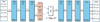 |
Fig. 3 Variational autoencoder used to create a K=5 dimensional latent space given the 23 × 5 values of the observed Δm|Δt histogram. The explanation of the network is very similar to the one in Fig. 2. |
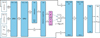 |
Fig. 4 Variational autoencoder used to create a K = 5 dimensional latent space given the 100 points of the folded light curve (phase ϕj ∈ [0, 1] and the standardised G-magnitude mj). The network does not receive the 100 phase values ϕj directly but rather the 100 × H values sin(2πhϕj), with h = 1, . . ., H and an equal number of values cos(2πhϕj). The first neural layer is a GRU to which the observations are fed sequentially (SEQ), i.e. 100 consecutive sets of size 1 + 2H corresponding to each time point of the light curve. The result is a matrix of size 100 × 128. Each of the 100 rows is then fed sequentially to the next GRU layer, resulting in a matrix of the same shape. The next layer takes each row of this matrix (of size 128), and computes an attention score corresponding to each point of the light curve. These scores are then used in a subsequent layer to compute a weighted average over the matrix rows, producing a feature set of size 128 where the time points that were deemed more important given the attention score receive a higher weight. In the final layers of the encoder, this feature set is then further reduced to the K = 5-dimensional latent coordinates (purple rectangles). The decoder works similarly as explained in Fig. 2, but now also receives the phase information (sin(2πhϕj), cos(2πhϕj)). The first decoding neural layer results in a matrix of size 100 × 128. Each row (of size 128) of this matrix is then fed to a neural layer, resulting again in a 100 × 128 matrix, which is then further reduced to a vector of size 100 by the final decoding layer, resulting in the 100 reconstructed (standardised) magnitudes of the folded light curve. |
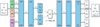 |
Fig. 5 Variational autoencoder used to further reduce the latent spaces produced by the networks illustrated in Figs. 2–4 (the green, orange, and purple rectangles) to a latent space of dimension 2, providing the coordinates (λ1, λ2) that are used for the interpretation in Section 9. Apart from the location in the 3K = 15-dimensional latent space, the VAE also receives the standard deviation of the G light curve, the colour estimate |
![Mathematical equation: $\[\overline{G_{\mathrm{BP}}}-\overline{G_{\mathrm{RP}}}\]$](/articles/aa/full_html/2025/09/aa54025-25/aa54025-25-eq18.png)
4.4 VAE to visualise the combined latent variables
For astrophysical interpretation, it is more convenient to use a 2D latent space, which can be directly visualised. We therefore introduced a final VAE to obtain two latent variables, λ1 and λ2, which combine the latent variables from the previous three VAEs along with additional features. These features are the standard deviation of the G band light curve σG, the logarithm of the estimated dominant frequency log10 f1 of the G band light curve and the colour estimate ![Mathematical equation: $\[\overline{G_{\mathrm{BP}}}-\overline{G_{\mathrm{RP}}}\]$](/articles/aa/full_html/2025/09/aa54025-25/aa54025-25-eq23.png) , i.e. the difference between the average magnitude in the GBP band and the GRP band light curves.
, i.e. the difference between the average magnitude in the GBP band and the GRP band light curves.
The architecture of this model is illustrated in Fig. 5 and further detailed in Appendix B. The model is trained using Eq. (3) with a Gaussian log-likelihood. No additional variance term is learned for this decoder. The results from this model are used to carry out the astrophysical analysis presented in Section 9. Contrary to other non-linear visualisation methods, the VAE produces an explicit function that maps the two spaces, a capability that is essential for efficiently scaling this method to the future larger Gaia DR4 dataset.
4.5 Optimisation and implementation details
The dataset described in Section 3.1 is randomly divided into training, validation, and test subsets, with proportions of 70%, 15%, and 15%, respectively. Models are trained iteratively for a maximum of 1000 epochs, with parameters initialised randomly using the He et al. (2015) scheme at the start of training. At the start of each epoch, the sources in the training subset are grouped into batches of size Nb = 256. Gradients of the cost function are computed for each batch, averaged, and used to update the model parameters using the Adam optimiser (Kingma & Ba 2015), an adaptive variant of stochastic gradient descent. The initial learning rate is set to 0.0001.
The validation subset is used to monitor the cost function during training. We apply early stopping with a patience of 15 epochs to avoid overfitting. The validation subset is also used to calibrate the most critical hyperparameters of the models, namely the dimensionality of the latent variables K and the trade-off between reconstruction and regularisation β. The selection of K is discussed in detail in the following section. The value of β is calibrated independently for each VAE through a grid search over [0.001, 0.01, 0.1, 1, 10]. The optimal values of β for the XP, Δm|Δt, folded light curve and 2D VAEs were found to be 1, 0.1, 0.01, and 1, respectively. Other hyperparameters are set to their previously defined values and left unmodified.
After the models have converged, the latent variables are evaluated through outlier detection, classification and clustering experiments performed using the test subset. To ensure robustness, each model is trained three times with different random initialisation seeds, and performance is reported as the average of metrics across these runs. All models are implemented using PyTorch (Paszke et al. 2019), version 2.4.1, and PyTorch Lightning (Falcon et al. 2020), version 2.4. The model implementation, training scripts and guidelines for obtaining the dataset and latent variables are available at https://github.com/IvS-KULeuven/gaia_dr3_autoencoder. The models are trained using an NVIDIA A4000 GPU. Table A.1 lists the computational time needed to obtain the latent variables for each of the described models. Using a single GPU, the latent variables of 100M sources can be obtained in a few hours, ensuring scalability to DR4.
 |
Fig. 6 Gaia DR3 source 4037765863920151040 XP mean spectra corresponding to a long period variable (first column). These data were compressed using the VAE and then reconstructed. The following columns show the reconstruction and the squared difference between the original and its reconstruction as the number of latent variables, K, increases. |
4.6 Latent variables assessment
Once the models are trained, the quality of the latent variables is evaluated through classification and clustering tasks. In the supervised classification tests, this evaluation is performed using logistic regression (LR) and a k-nearest neighbours (k-NN) classifier. The LR is a linear model that predicts class probabilities based on a weighted combination of the input features, making it simple yet effective for assessing linear separability. The k-NN classifier, on the other hand, is a non-parametric method that assigns labels based on the majority class of the k nearest points in the latent space, providing insight into the local structure of the learned representation. We deliberately restrict this evaluation to simple classifiers because our primary goal is to assess the structure and informativeness of the latent variables. More complex classifiers, such as Random Forest or XGBoost, would likely achieve better classification performance, but they might also compensate for limitations in the learned representation.
The LR and k-NN classifiers are implemented using the scikit-learn library (Pedregosa et al. 2011). The training and validation partitions that were used to train the AEs are also used to fit and select the optimal hyperparameters. Specifically, the level of regularisation for LR and the number of neighbours for k-NN are tuned during this process. The input to the classifiers include the mean of the latent variables, the uncertainty of the XP and G band folded light curve decoders, σXP and σF, the standard deviation of the G band light curve σG4 and the estimated fundamental frequency f1. The classifiers’ performance is evaluated on the test partition, which consists of the sources that were not used during the training of the VAEs and the classifiers.
By defining nij as the number of sources labelled as class i and predicted as class j, the performance of the classifier is visually assessed using row-normalised confusion matrices, where the cell in the i-th row and j-th column corresponds to nij/ Σj nij. Performance for a given class c is summarised using F1−scorec, which is the harmonic mean between precisionc, i.e. the proportion of correctly classified sources out of all sources predicted as belonging to c and recallc, i.e. the proportion of correctly classified sources out of all actual sources of class c.
As the distribution of classes in the labelled subset is highly unbalanced, performance summaries for the entire test partition are presented using both macro and weighted averages. The macro average computes the unweighted mean of the F1−scores across all classes, allowing minority classes to have a significant influence on the overall score. In contrast, the weighted average takes into account each class’s F1−score according to its proportion in the dataset, meaning the overall score is more heavily influenced by the performance on the majority classes. The F1 macro is used to select the best model in cross-validation.
5 Selecting the dimensionality of the latent space
Among the hyperparameters of the VAE, the dimensionality of the latent variable vector, K, has the most significant influence on the results and we analyse its impact in this section. K controls the amount of compression that an AE applies to the data. A higher K allows the encoder to obtain more informative representations, leading to better reconstructions. However, choosing K requires a balance: too small a value results in a latent space with limited or no discriminative power, while too large a value risks overfitting to noise in the data, enabling near-perfect reconstructions at the expense of the usefulness of the latent variables for classification, clustering and other downstream tasks.
Figure 6 illustrates how the reconstruction of the XP mean spectra for a given Gaia DR3 source evolves with K. Even with just two latent variables, the reconstruction captures the general shape and relative differences between the BP and RP spectra, although key details are smoothed out. In contrast, the reconstructions with K = 5 and K = 10 are much closer to the original spectra, with only marginal differences between them, as reflected in the errors. Figure 7 shows an example of the compression of a folded G band light curve of an eclipsing binary star. With K = 2, the reconstruction fails to capture the correct shape, defaulting to a sinusoidal curve, probably the most common pattern found in the dataset for this modality. In contrast, K = 5 and K = 10 accurately capture the shape of the light curve, including the distinctive features of the eclipses. Similar to what was observed for the XP mean spectra, the difference between the K = 5 and K = 10 reconstructions is marginal.
For the evaluation of K, we consider two metrics measured in the validation partition of our dataset. The first is the average between the ELBOs (Eq. (3)) from the VAEs of the XP mean spectra, Δm|Δt and G band folded light curve. The ELBO takes into account the likelihood of the reconstructed data, and hence, we expected it to increase with K. Although not optimal, we adopt the same number of latent variables for each VAE to facilitate the analysis. The second metric is the macro F1−score measured through a LR classifier using the combined latent variables as described in Section 4.6. We use this downstream task to measure the discriminative power of the latent variables, which, contrary to the likelihood, is not expected to always increase with K. Figure 8 illustrates these two metrics as K is increased from two to ten. The validation ELBO shows increments above the error bars up to K = 8. Not growing beyond this value is due to the influence of the regularisation term in Eq. (3). The first five latent variables contribute most to this metric. Similarly, the F1−score rises sharply up to K = 5, after which it levels off. This suggests diminishing returns in both reconstruction quality and classification performance for higher values of K. Using fewer latent variables also facilitates the interpretation. Based on these results, we select K = 5 for the remainder of our analysis.
 |
Fig. 7 Folded G band light curve of Gaia source DR3 5410617628478565248 corresponding to an eclipsing binary (first column). These data were compressed using the VAE and then reconstructed. The following columns show the reconstruction and the squared difference between the original as K increases. |
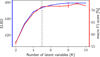 |
Fig. 8 Average ELBO (in blue) and macro F1−score (in red) in the validation set as a function of the number of latent variables (K). Higher is better for both metrics. A black dashed line marks K = 5. |
6 Identification of outliers using the latent variables
In this section, we show that the latent space produced by our ANN can be used to identify outliers or anomalous sources. One important application of this capability is quality control of the variability classifications performed by DPAC-CU7, in which several of the current authors are involved. Given the immense size of the datasets, these classifications are often carried out using automated algorithms. Consequently, there is significant interest in exploring whether part of the verification process can also be automated.
As an example, we consider the 7431 sources from the vari_rrlyrae table that are included in the test partition of our dataset. This table, compiled through a rigorous analysis by Clementini et al. (2023), contains a clean catalogue of RR Lyr stars. The aim is to identify the most atypical RR Lyr sources using the latent variables as input for an outlier detection algorithm. Specifically, we used the local outlier factor (LOF) algorithm (Breunig et al. 2000), which assigns a score indicating how isolated a source is relative to its local neighbourhood. The larger the LOF, the more isolated the source is; inliers tend to have values close to one. The scikit-learn implementation of LOF with its default hyperparameters is used. As input, we consider the five latent variables derived from the folded G band time series, i.e. the outliers are to be interpreted as the most atypical in the latent space of the folded time series. However, the same procedure outlined here can be applied to the other latent variables to identify the most atypical in the XP or Δm|Δt representations.
A widely used heuristic for anomaly detection that is specific to AEs consists of using the quality of the reconstructed data to identify outlier examples. This assumes that anomalous sources are harder to reconstruct because the model minimises the overall reconstruction error, thereby prioritising normal instances (Pang et al. 2021; Sánchez-Sáez et al. 2021). In this case, this corresponds to identifying sources for which the decoder variance ![Mathematical equation: $\[\sigma_{F}^{2}\]$](/articles/aa/full_html/2025/09/aa54025-25/aa54025-25-eq24.png) is large. In what follows, we use both the LOF and
is large. In what follows, we use both the LOF and ![Mathematical equation: $\[\sigma_{F}^{2}\]$](/articles/aa/full_html/2025/09/aa54025-25/aa54025-25-eq25.png) to identify outlier candidates and analyse the differences between these approaches.
to identify outlier candidates and analyse the differences between these approaches.
Figure 9 shows the LOF versus ![Mathematical equation: $\[\sigma_{F}^{2}\]$](/articles/aa/full_html/2025/09/aa54025-25/aa54025-25-eq26.png) distribution for the 7431 sources from Clementini et al. (2023) in the test set partition of our training set. Most sources are concentrated around LOF values close to one and have low
distribution for the 7431 sources from Clementini et al. (2023) in the test set partition of our training set. Most sources are concentrated around LOF values close to one and have low ![Mathematical equation: $\[\sigma_{F}^{2}\]$](/articles/aa/full_html/2025/09/aa54025-25/aa54025-25-eq27.png) . In general, the correlation between LOF and
. In general, the correlation between LOF and ![Mathematical equation: $\[\sigma_{F}^{2}\]$](/articles/aa/full_html/2025/09/aa54025-25/aa54025-25-eq28.png) is weak, i.e. the most isolated sources are not necessarily due to the model being unable to reconstruct them correctly. The three sources with the highest LOF values are marked with stars. Notably, these sources also exhibit low values of
is weak, i.e. the most isolated sources are not necessarily due to the model being unable to reconstruct them correctly. The three sources with the highest LOF values are marked with stars. Notably, these sources also exhibit low values of ![Mathematical equation: $\[\sigma_{F}^{2}\]$](/articles/aa/full_html/2025/09/aa54025-25/aa54025-25-eq29.png) , suggesting that their reconstructions are reliable. The folded light curves of these sources are shown in the left panel of Fig. 10, ranked by their LOF from top to bottom. The shape of the light curves suggests that these sources are likely eclipsing binaries. This is further confirmed using the amplitude ratio between the GBP and GRP band time series, as indicated by Clementini et al. (2023). Moreover, the second and third sources have been classified as binaries using ATLAS data (Heinze et al. 2018). The full potential of latent-space neighbour analysis for identifying contaminants in Gaia data will be examined in greater detail in Wyrzykowski et al. (in prep.).
, suggesting that their reconstructions are reliable. The folded light curves of these sources are shown in the left panel of Fig. 10, ranked by their LOF from top to bottom. The shape of the light curves suggests that these sources are likely eclipsing binaries. This is further confirmed using the amplitude ratio between the GBP and GRP band time series, as indicated by Clementini et al. (2023). Moreover, the second and third sources have been classified as binaries using ATLAS data (Heinze et al. 2018). The full potential of latent-space neighbour analysis for identifying contaminants in Gaia data will be examined in greater detail in Wyrzykowski et al. (in prep.).
The second column of Fig. 10 shows the three sources with the highest decoder variance, representing those that the model struggles to reconstruct accurately. These sources have very noisy periodograms, which complicates the extraction of the correct frequency and leads to finding a high-frequency alias instead, resulting in a seemingly random pattern in the folded light curve. Analysis using the amplitude ratio between the GBP and GRP band time series suggests that these sources are indeed RR Lyr stars. Moreover, the first and third sources have been classified as RR Lyr stars using ATLAS data. In contrast to the LOF method, the candidates identified using ![Mathematical equation: $\[\sigma_{F}^{2}\]$](/articles/aa/full_html/2025/09/aa54025-25/aa54025-25-eq34.png) are not contaminants from other astrophysical classes. Instead, they primarily result from noisy time series or preprocessing errors. Nonetheless, combining both metrics may offer added value. This will be explored in future work.
are not contaminants from other astrophysical classes. Instead, they primarily result from noisy time series or preprocessing errors. Nonetheless, combining both metrics may offer added value. This will be explored in future work.
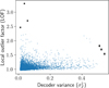 |
Fig. 9 Local outlier factor vs the variance of the G band folded light curve decoder ( |
![Mathematical equation: $\[\sigma_{F}^{2}\]$](/articles/aa/full_html/2025/09/aa54025-25/aa54025-25-eq30.png)
![Mathematical equation: $\[\sigma_{F}^{2}\]$](/articles/aa/full_html/2025/09/aa54025-25/aa54025-25-eq31.png)
![Mathematical equation: $\[\sigma_{F}^{2}\]$](/articles/aa/full_html/2025/09/aa54025-25/aa54025-25-eq32.png)
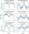 |
Fig. 10 Folded light curves (black dots) and their reconstructions (blue) for the three sources in the RR Lyr SOS table with highest LOF (left panels) and highest |
![Mathematical equation: $\[\sigma_{F}^{2}\]$](/articles/aa/full_html/2025/09/aa54025-25/aa54025-25-eq33.png)
Supervised classification results in the latent space.
7 Supervised classification in the latent space
The latent space was constructed in a self-supervised way without any variability class labels known from the literature. Although it primarily serves to discover unanticipated overdensities, one could ask if the 3K = 15 coordinates of the latent space can also be used as new features for supervised classification. To verify this, we perform a classification experiment using the 38 740 labelled sources described in Section 3.2. Table 1 presents the test set F1−scores achieved by the LR and the k-NN classifiers (see Section 4.6) trained on different subsets of the latent variables. We present results where the classifiers were applied to (1) the K latent variables coming from the XP spectra, (2) the K latent variables coming from the Δm|Δt distribution, (3) the K latent variables coming from the folded light curves, (4) the 2K latent variables coming from both the folded light curves and the Δm|Δt distribution combined, and 5) all the 3K latent variables combined.
The classifiers show comparable performance for the single-modality K input latent variables, except for the XP mean spectra, where k-NN significantly outperforms LR. This indicates that the latent space of the XP spectra contains intricate local structures that cannot easily be linearly separated. For the LR classifier, the best single-modality performance is achieved by the G band folded light curves. Across both classifiers, the best performance is observed when all latent variables are combined, highlighting the advantages of a multimodal approach. Even though both classifiers achieve a similar 81% weighted F1−score, the LR slightly outperforms the k-NN in terms of macro F1−score, meaning that the former handles the minority classes better without affecting the overall performance. In what follows, we perform a comparison at the individual class level, focusing on the results of the LR classifier.
Figure 11 shows the test set confusion matrices of the LR classifier trained using different combinations of latent variables. Through these figures, we can see that the performance across classes varies considerably depending on the modality. From the results of the XP VAE, shown in Fig. 11a, we observed the following:
The WDs are almost perfectly separable despite being indistinguishable from other classes in the light curve associated modalities.
Most LPVs are correctly recovered. The sources classified as an LPV are characterised by their strong red spectra.
The SPB stars are the primary source of misclassification for ACV|CP and β Cep stars. Conversely, the most significant source of confusion for the SPB stars are ACV|CP and β Cep stars. Additionally, β Cep stars are the leading source of misclassification for BE|GCAS. All these classes are characterised by their strong blue spectra.
The results from the Δm|Δt VAE, shown in Fig. 11b, reveal interesting patterns despite notable contamination among rotational and eruptive variables. For example,
Most RR Lyr ab and RR Lyr c stars are correctly recovered due to their constrained period range. RR Lyr d stars, which pulsate in double mode, are mostly confused with the former.
δ Cep and t2 Cep stars are confused for one another as well as for LPVs. The period range of the classes partially overlap. Furthermore, some AGN and CVs are also misclassified as LPV. All of these sources are characterised by variability on long timescales.
Most ECLa are correctly recovered. This is due to the model capturing the pattern of the top and bottom magnitude bins being filled by the sharp eclipses of these sources.
The results from the folded light curve VAE, shown in Fig. 11c, also show interesting properties:
The ECL yield recalls above 50%, with most of the contamination confined to their sub-classes. This demonstrates the model’s ability to effectively capture the distinctive phase patterns of these sources.
The majority of Cepheid and RR Lyr stars are accurately classified. As with the ECL, these classes also have distinct and recognisable phase patterns.
There is significant misclassification between SOLAR, YSO, SPB, ACV|CP, β Cep and γ Dor stars. The folded light curves of these sources exhibit shapes resembling noisy sine waves.
AGNs are frequently misclassified as YSOs, WDs, and LPVs. Similarly, LPVs are often misclassified as YSOs and AGNs. For non-periodic and semiregular variables, the estimated periods are, in most cases, related to Gaia scan-angle dependent signals (Holl et al. 2023).
Figure 11d shows the results of the LR classifier using the latent variables from all modalities as input. For reference, the precision, recall, and F1−scores per class for this classifier are listed in Table A.2. Performance is superior to the individual modalities across all individual classes, which is reflected in the strong diagonal of the confusion matrix. The following classes exhibit a relative increase in F1−score of more than 50% with respect to the best single modality: β Cep stars, γ Dor stars, ELL, RS, SPB, RR Lyr d stars, t2 Cep, CV and YSO.
Some classes remain challenging to classify correctly:
RS, ELL, and YSO: These classes are confused between them and with the SOLAR class. RS, ELL and SOLAR are all examples of rotational variables. Confusion between these classes was also reported by Rimoldini et al. (2023) (see Table 3).
SPB: Approximately 20% of sources from this minority class are missclassified as ACV|CP. Conversely, a notable fraction of ACV|CP, and β Cep stars are erroneously predicted as SPB. All these classes share similar XP properties and periodicities. Confusion between SPB and ACV|CP was also reported by Rimoldini et al. (2023).
RR Lyr d stars, which are multimode pulsators, are difficult to distinguish from other members of their parent class. A similar situation can be observed for ECLb. The folded light curve morphology of ECLb is a transition between ECLa and ECLw and this is captured by the latent variables.
Next, we compare the latent variables against the classifications published in Gaia DR3 (Rimoldini et al. 2023). These were obtained using an ML classifier trained with labels similar to those employed in this study (Gavras et al. 2023), but with notably different inputs: the Gaia DR3 classifier did not utilise information from the XP mean spectra (but it did use astrometric features). Moreover, the DR3 predictions were refined through post-processing based on attribute filters to enhance the reliability of the classifier’s results.
This comparison is carried out using a subset of 3300 sources obtained by removing from our test set all the sources that Rimoldini et al. (2023) used for training. The results presented in Table 2 show overall agreement between the two, though significant differences arise in some of the classes, such as ACV, CEP, SOLAR and YSO. However, given the limited sample size, these differences may not be fully representative of the broader dataset. Notably, both models are not able to recover the RS sources in this sample.
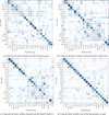 |
Fig. 11 Confusion matrices for the test partition sources of the labelled subset. The rows correspond to the ground truth class selected from Gavras et al. (2023), and the columns to the class predicted by the classifier using the latent variables as input. The cell in the i-th row and j-th column gives the percentage of sources labelled as class i and predicted as class j with respect to the total number of sources of class i. Each matrix represents the averaged results of a linear classifier trained on different sets of latent variables. Standard deviations are shown after the | symbol. Percentage rates and corresponding standard deviations below 1% are not shown for clarity. |
Comparison between VAE and DR3 classifications.
8 Analysis of clusters in the latent space
Our aim at this point is to identify and extract in an automated way the different clusters present in the 3K = 15-dimensional latent space. We explore their content by using the 301 778 test set sources with labels from Rimoldini et al. (2023).
We begin by evaluating the k-means algorithm for clustering the latent variables. k-means was selected due to its computational efficiency, which is essential for application to the significantly larger dataset expected for Gaia DR4. In this case, we set the number of clusters to 17, as it yields the minimum Davies-Bouldin index (Davies & Bouldin 1979) as shown in Fig. A.7.
The top panel of Fig. 12 presents the resulting confusion matrix between the reference labels and the k-means clusters. Each row displays the distribution of a given variability class across the clusters (recall). To aid visualisation, clusters are sorted by the dominant class within them, marked with red lines. For example, the first cluster is dominated by AGNs, with contamination from CVs, BE|GCAS and WDs. The confusion matrix reveals that more than half of the clusters are dominated by three classes. This is consistent with the imbalanced distribution of classes in the subset, where SOLAR_LIKE, LPV, and ECL make up 40%, 20%, and 13% of the dataset, respectively.
As a second clustering method, we considered a Gaussian mixture model (GMM) with full covariance matrices. The marginal likelihood for this model is defined as
![Mathematical equation: $\[L(\boldsymbol{\pi}, \boldsymbol{\mu}, \boldsymbol{\Sigma})=\sum_i \sum_{c=1}^C \pi_c \mathcal{N}(x_i {\mid} \mu_c, \Sigma_c),\]$](/articles/aa/full_html/2025/09/aa54025-25/aa54025-25-eq35.png) (12)
(12)
where π are the mixture coefficients and C is the number of clusters. k-means can be considered as a special case of GMM, where ![Mathematical equation: $\[\pi_{c}=\frac{1}{C}\]$](/articles/aa/full_html/2025/09/aa54025-25/aa54025-25-eq36.png) , i.e. equal density, and Σc = σ2I, i.e. a shared spherical covariance. While GMMs are computationally more complex than k-means and are unlikely to scale efficiently for the larger Gaia DR4, their increased flexibility offers the potential to better handle class imbalance.
, i.e. equal density, and Σc = σ2I, i.e. a shared spherical covariance. While GMMs are computationally more complex than k-means and are unlikely to scale efficiently for the larger Gaia DR4, their increased flexibility offers the potential to better handle class imbalance.
The bottom panel of Fig. 12 shows the resulting confusion matrix between the reference labels and the GMM clusters. Compared to k-means, the GMM reduces the dominance of the majority class (SOLAR_LIKE), enabling better representation of medium-sized classes such as CEP (0.2%) and RR (2%). The RS class (10%), despite being adequately represented in terms of examples, cannot be distinguished from the SOLAR_LIKE class. In general, classes such as RS, SPB, and ELL, which were incorrectly classified in the supervised experiments, exhibit similar behaviour in the clustering scenario. While medium-sized classes show improvement over the k-means results, very small classes such as β Cep, CV and WD5 remain intermingled as contaminants within larger clusters. Increasing the number of clusters to 100 allows for the identification of pure clusters associated with these classes, but at the cost of making the clustering results impractical to use and interpret. In what follows, we describe the clusters found by GMM:
Cluster 1 contains the majority of AGNs with slight contamination from BE|GCAS.
Cluster 2 is dominated by BE|GCAS with contamination from ACV|CP, β Cep stars, SPBs and WDs. All of these sources are characterised by their strong blue spectra, as inferred from the reconstruction of the cluster mean (Fig. A.8a).
Cluster 3 contains the majority of Cepheids.
Clusters 4 and 5 are dominated by δ Sct |γ Dor stars, where cluster 4 is much purer. Interestingly, cluster 5 showcases the same contaminants as cluster 2. The reconstruction of the mean of cluster 5 (Fig. A.8b) suggests that these sources vary more rapidly than those in cluster 2.
Clusters 6 to 9 are ECL clusters. Cluster 6 is contaminated with several other classes. Other ECL clusters exhibit high purity.
Clusters 10 to 12 are LPV clusters with different degrees of contamination, mainly from YSO, ELL, CVs and Cepheids.
Clusters 13 and 14 are pure RR Lyr star clusters. The reconstructions from the means of these clusters (Figs. A.8c–A.8d) suggest that they are associated with RR Lyr ab and RR Lyr c stars, respectively.
The last three clusters are dominated by SOLAR_LIKE with high contamination from RS and YSO. This is similar to what was observed in the supervised analysis.
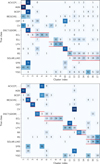 |
Fig. 12 Clustering results of the latent variables organised into 17 groups using k-means (top panel) and a Gaussian mixture model with full covariance (bottom panel). Rows show the distribution of the classes across the clusters (rows add up to 100). Red lines highlight the class that constitutes the majority within each cluster. |
9 Astrophysical interpretation of the latent space
In this section, we analyse in more depth the most important regions and overdensities in the latent space from an astrophysical point of view. We work in the 2D latent space shown in Fig. 13 produced by the ANN described in Fig. 5, rather than the 3K = 15-dimensional latent space, as the former is easier to visualise. Our analysis uses the 38 740 sources of Gavras et al. (2023) for which a variability class label is available (see Section 3) as well as the set of sources for which the SOS catalogues in Gaia DR3 published a class label. For a first identification of the different overdensities in Fig. 13, we divided the latent space into bins, and we provide the most frequently occurring variability class for each bin in Fig. 14. The colour code indicates the fraction of stars in the bin that have the shown label. Despite the fact that the ANN does not have access to the published class label, many of the known variability classes are well separated in the latent space. Moreover, not only are the majority of bins with the same class label grouped together, variability classes that are expected to be similar or overlapping (e.g. eclipsing EA, EB, and EW stars) have bins close to each other, while sources that a human classifier would set apart, e.g. white dwarfs (WD) and long-period red giants (LPV) are positioned at opposite sides of the latent space.
Some Gaia sources have time series that show calibration-induced spurious variability, introduced by an incomplete modelling of the on-sky source structure (e.g. multiple unresolved sources or extended objects like galaxies), resulting in a scan angle dependent signal (Holl et al. 2023). Figure A.13 plots the known such sources and shows that the centre of the latent space is particularly affected, which is the reason that the centre bins of Fig. 14 do not show a class label.
In the subsections below, we investigate some of the overdensities in the latent space by overplotting them with sources for which we have a variability class label as outlined in Section 3.
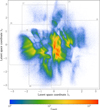 |
Fig. 13 Distribution of the 4 136 544 sources in the 2 D latent output space of our ANN designed to perform an unsupervised clustering of variable sources (see Section 4 and Fig. 5 for more details). Different overdensities of points correspond to different (sub)types of variability. A first identification of the overdensities can be found in Fig. 14. For future reference we also depict the parts of this latent space shown in Figs. 15–20 with rectangles and provide the figure number is in one of the corners. |
 |
Fig. 14 Most frequently occurring variability class for each bin of the latent space shown in Fig. 13 for the set of variable stars that have a variability class label available (see Section 3). The bins are colour-coded with the fraction of stars in the bin that have the shown label. Only the variability classes SPB, γ Dor, β Cep, δ Sct, CP stars, AGNs, LPVs, RR Lyr (ab, c, and d), Cepheids, WDs, eclipsing binaries (EA, EB, EW), ELL variables, Be (BE) variables, and YSO variables were taken into account to generate this figure. |
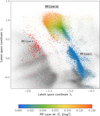 |
Fig. 15 Region of the latent space where the RR Lyr stars are located. The RR Lyr variables for which a “RRab” classification label was available in the Gaia DR3 catalogue are overplotted in colour, where we used the pulsation amplitude A11 for the colour scale. The RR Lyr c and RR Lyr d variables are plotted in blue resp. red. |
9.1 RR Lyr stars
The overdensities in the latent space around coordinates (λ1, λ2) = (−1.3, 0.9) relate to RR Lyr variables. A close-up of this region is shown in Fig. 15, where we overplotted the sources with an RR Lyr variability class label from the literature. The ANN separates the three different subgroups of RR Lyr (ab, c, and d). The RR Lyr d variables occupy the same region as the δ Sct and γ Dor variables. For the sake of conciseness, we used two different quantities for the colour scales to overplot the RR Lyr ab and RR Lyr c samples. The colour of the RR Lyr ab variables relates to the amplitude A11 of the first harmonic of the main frequency as published in the Gaia DR3 SOS variability catalogue (see Clementini et al. 2023, for more details). A significant gradient of this amplitude can be seen, explaining the extent of the RR Lyr ab cluster in the latent space. The RR Lyr ab cluster contains two substructures best seen in Fig. 16 around (λ1, λ2) = (−1.4, 0.9). We discuss this in more depth in Appendix A, in which we provide support for the hypothesis that the well-known Oosterhoff dichotomy is the underlying reason. Finally, we mention that the RR Lyr c variables extend from close to the RR Lyr ab variables down to the region in the latent space where the eclipsing binaries are located (see the subsection on eclipsing binaries below).
 |
Fig. 16 Sources for which we have a γ Dor or a white dwarf classification label from the literature are shown in red and orange, respectively. For the known δ Sct variables, we used a colour scheme that shows the standard deviation in the Gaia G passband as a proxy for the oscillation amplitude. We indicate the position of the high-amplitude δ Sct stars (HADS), with amplitude above 100 mmag. |
9.2 δ Sct stars, γ Dor stars, and white dwarfs
The location of the δ Sct stars in the latent space is close to that of the RR Lyr stars and the γ Dor stars. Figure 16 offers a zoom of the relevant region in the latent space, in which we highlighted those sources for which we have a δ Sct variability label from the literature (see Section 3). The colour scheme represents the standard deviation in the Gaia G light curve which serves as a proxy for the oscillation amplitude. We indicate the location of the high-amplitude δ Sct stars (HADS) in the plot, close to the RR Lyr stars. The low-amplitude δ Sct stars (in dark blue), well separated from the HADS, are close to the γ Dor stars (in red), and partly overlap with them. This is expected from an astrophysical point of view, given that they have similar folded light curves and are only slightly redder. The main way to distinguish them is the oscillation frequency (long period g-modes versus short-period p-modes), but in practice overlap is expected. Indeed, hybrid pulsators which show both p- and g-mode oscillations with overlapping frequencies due to fast rotation are common (Aerts 2021; Aerts & Tkachenko 2024). In addition, the Gaia time sampling is such that a γ Dor frequency can be aliased into the δ Sct frequency domain and vice versa (Gaia Collaboration 2023a; Hey & Aerts 2024).
The white dwarf oscillators occur as a separate group in Fig. 16. The Gaia time sampling is too coarse to detect the high-frequency oscillations (P ≈ 10 min), so this clustering is based on their distinct XP spectra. This is supported by the difference in classification performance between the individual modalities (Section 7).
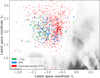 |
Fig. 17 Region of the latent space where the variable B stars are projected. The β Cep, SPB, and CP variables for which we have a classification from the DPAC-CU7 training set mentioned in Section 3 are plotted in colour. |
9.3 Hot variable stars
The variable B stars occupy a separate region in the latent space around (λ1, λ2) = (−1.0, 2.3). In Fig. 17 we show a zoom of this region, and overplot the β Cep stars, SPB, and CP stars from the Gaia DR3 training set as outlined in Section 3.
The β Cep stars and SPB variables largely overlap in the latent space, although the former occur predominantly at lower λ1 coordinates in this region, which is mainly correlated with the main frequency f1 as illustrated in Fig. A.11. This overlap is not an artefact of projecting the data in a 2D latent space. Section 7 reveals that also in the 15D latent space it is hard to separate the SPB variables with the current dataset. This is in line with the results from Mombarg et al. (2024) and Fritzewski et al. (2025), who found large populations of hot g–mode and hybrid p– / g–mode pulsators to occupy an uninterrupted area along the main sequence, stretching all the way from the γ Dor stars up to the β Cep instability strip.
The CP stars occupy the same region in the latent space but are more concentrated towards higher λ1 and λ2 values. The reason that the ANN is able to discriminate between them is that they more frequently have a late B or early A spectral type and are therefore redder than many pulsating B stars, which the ANN picks up through the XP spectra. In addition, CP stars can show variability at longer time scales in the Δm|Δt histogram, related to their rotation period, thus differentiating them from the short-period β Cep stars. It is well known that CP stars and SPB pulsators occupy the same region in the Hertzsprung-Russell diagram (Briquet et al. 2007).
9.4 Eclipsing binary stars
The overdensities in the 2D latent space around (λ1, λ2) = (−0.5, −1.4) are dominantly occupied by binary stars as shown in Fig. 14. The substructure in that region is largely determined by the morphology of the (folded) light curve. To demonstrate this, we follow Mowlavi et al. (2023) who used a simple but effective model to characterise the variability of Gaia DR3 binary candidates. In their work, the eclipses were modelled using two Gaussian functions, while an ellipsoidal variation was modelled with a cosine function. In Figs. 18, A.14 and A.16, we plot for the binary candidates in their catalogue, respectively, the magnitude difference between two consecutive eclipses, the duration of the primary eclipse as a fraction of the orbital period, and the amplitude of the cosine component (if any), which serves as a proxy for the amplitude of the ellipsoidal variation.
These figures show that the overdensity in the bottom relates to eclipsing binaries of type EA with clearly detached eclipses and no ellipsoidal variation. The magnitude differences between the eclipse depths range from 0 to more than 200 mmag, but there is no clear gradient present. Visual inspection of the folded light curves of the sources revealed that this region also includes sources for which outliers were incorrectly interpreted as eclipses and for which the folded light curve does not show the expected morphology of a type EA eclipsing binary. This had an impact on the performance of the ANN in substructuring this type of binaries. Points flagged by DPAC-CU7 as unreliable and points with large uncertainties were removed during preprocessing. No other outlier-removing procedure was applied to avoid that eclipses would be erroneously removed.
In the centre of the binary region, the ANN places the EB binaries with detached eclipses, but for which Fig. A.16 shows a detectable variation outside the eclipses. The ANN shows a gradient in the amplitude of the ellipsoidal variation, increasing from left to right. The top part of the region is occupied by the close over-contact EW binaries for which Fig. A.14 shows that the eclipses take a large fraction of the orbital period and with a continuous variation outside of the eclipses. The colour map in Fig. 18 shows that most systems have either equal or similar minima.
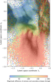 |
Fig. 18 Part of the latent space where the ANN projects eclipsing and ellipsoidal binaries. The grey background shows the same density as in Fig. 13. Sources that were published in the Gaia DR3 Variability catalogue gaiadr3.vari_eclipsing_binary are overplotted in a 2D histogram of small hexagons where the colour of each hexagon corresponds to the average magnitude difference between primary and secondary eclipses of the sources inside that bin. |
9.5 Long-period variables
Figure 14 shows that most of the area defined by λ1 > 0.3, λ2 < 2 in the latent space is occupied by LPVs, such as Mira and red semi-regular variables. Figure 13 shows substructure in the density in that region. In Fig. 19 we show a zoom of this region, and overplot the LPV candidates published in Gaia DR3 (table gaiadr3.vari_long_period_variable, selecting G ≤ 19) with a classification of LPV/C or LPV/O rich. The colour coding was done using the quantity ⟨Δλ⟩RP which is published as scikit-learnmedian_delta_wl_rp in the same table. This quantity is the difference in pseudo-wavelength between the two highest peaks in the Gaia RP spectrum, and probes the existence of particular molecular bands. It allows for the detection of carbon stars (C stars), which show strong imprints of carbon-based molecules such as CN or C2 in their spectrum, in contrast with oxygen-rich LPVs, which show molecular bands of TiO and VO. Lebzelter et al. (2023) identify the interval ⟨Δλ⟩RP ∈ [7, 11] and G ≤ 19 as reliable criteria to select C stars. This corresponds to the group of orange points in the latent space. The ANN was never given the value of ⟨Δλ⟩RP, so the fact that the C stars form an isolated cluster in the latent space implies that the ANN was able to recognise the relevant feature in the Gaia RP spectrum.
Sources with ⟨Δλ⟩RP ≤ 7 are identified by Lebzelter et al. (2023) as oxygen-rich LPVs. The ANN separates well the sources with ⟨Δλ⟩RP ≈ 6 (yellow in Fig. 19) from the sources with ⟨Δλ⟩RP ∈ [2, 5] (greenish) in the latent space. Figure 5 in Lebzelter et al. (2023) shows that values of ⟨Δλ⟩RP between 4 and 5 can be caused by ZrO bands in addition to TiO bands, occurring for S stars. Sources at ⟨Δλ⟩RP ≥ 12 were identified by these authors as originating from a molecular band at shorter wavelengths identified as the second largest peak in the RP spectrum. Although they occur in a large part of the LPV region in the latent space, the ANN does produce an overdensity with a strong concentration of these stars.
Figure A.15 shows the same LPV region in the latent space, but this time colour-coded with the main period P1 found in the Lomb-Scargle periodogram. The ANN used this information to insert further structure in the overdensities. In particular, the Mira variables with long periods (red points) appear at larger values of λ1. The blue dots are sources for which a main frequency f1 ≈ 12 d−1 originating from Gaia’s scanning law was found, so it is doubtful whether the overdensity at the left of the region has an astrophysical origin.
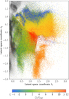 |
Fig. 19 Part of the latent space where the ANN projects the long period variables. The grey background shows the same density as in Fig. 13. In colour, we overplotted the sources which were published in the Gaia DR3 Variability catalogue as a candidate O-rich or C-type LPVs. The quantity ⟨Δλ⟩RP was taken from the same catalogue (column name median_delta_wl_rp) and probes particular molecular bands in the RP spectrum (see text). |
9.6 Active galactic nuclei
As already shown by the substructure in Fig. 13, the variable AGNs form a fairly isolated cluster around latent coordinates (λ1, λ2) = (0.25, 2.0). However, as discussed at the beginning of this Section, the extendedness of the AGNs is a known origin of spurious scan-angle dependent signals. Much of the same substructures can therefore also be found in Fig. A.13, containing known sources with a spurious signal, in particular the overdensity around (λ1, λ2) = (0.1, 1.6). Although AGNs are usually not periodic, we computed the main frequency f1 for each AGN candidate published in Gaia DR3 (table gaiadr3.vari_agn, see Carnerero et al. 2023 for details), and plotted the result in Fig. 20. This figure shows that the main overdensity originates from sources having f1 = 12 d−1, originating from Gaia’s scanning law.
The group of points coloured green in Fig. 20 contain sources with a main period listed in Holl et al. (2023) relating to Gaia’s scanning law, for example ![Mathematical equation: $\[P_{1}=f_{1}^{-1}=13.4 \mathrm{~d}, 16.3 \mathrm{~d}, 25.0 \mathrm{~d}\]$](/articles/aa/full_html/2025/09/aa54025-25/aa54025-25-eq37.png) , and 31.5 d. The blue sources in Fig. 20, on the other hand, show a main frequency that is consistent with the low-frequency red noise that is typical for AGNs. The ANN projected the vast majority of AGN candidates published in Gaia DR3 in the same region in the latent space, independently confirming their candidate status, even the ones where the highest peak in the Fourier spectrum is instrumental. However, care needs to be taken when analysing overdensities. If the observed data still contains instrumental features, the ANN will likely pick it up, resulting in spurious overdensities in the latent space.
, and 31.5 d. The blue sources in Fig. 20, on the other hand, show a main frequency that is consistent with the low-frequency red noise that is typical for AGNs. The ANN projected the vast majority of AGN candidates published in Gaia DR3 in the same region in the latent space, independently confirming their candidate status, even the ones where the highest peak in the Fourier spectrum is instrumental. However, care needs to be taken when analysing overdensities. If the observed data still contains instrumental features, the ANN will likely pick it up, resulting in spurious overdensities in the latent space.
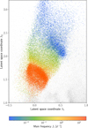 |
Fig. 20 Region of the latent space occupied by AGNs. For the AGN candidates published in the Gaia DR3 release, we colour-coded the frequency with the highest amplitude found in the Lomb-Scargle frequencygram computed from the light curves in the Gaia G passband. |
10 Conclusions
In this work, we have presented a self-supervised ML methodology based on VAEs to derive latent representations of variable sources. Our evaluation of the latent variables using Gaia DR3 data demonstrates that the VAEs effectively encode the characteristic variability patterns, thus enabling downstream applications such as classification and clustering. These models extract information from two modalities, namely, epoch photometry and low-resolution XP mean spectra. Our classification experiments show that there is a significant beneficial synergy when these Gaia DR3 products are used together. Notable examples include the improvement in F1−score for classes such as β Cep and γ Dor stars, which were highly contaminated in single-modality setups. The latent variables also prove effective in detecting atypical sources. This was exemplified with RR Lyr stars, where the latent representations successfully highlighted atypical sources, which were found to correspond to misclassifications or issues arising from a wrong estimation of the period. Our preliminary results will be expanded in the future, as we expect this capability to be particularly useful for Gaia DR4. Clustering results also show that partitioning the latent space allows for the recovery of the known major variability classes, but handling dataset imbalance remains a challenge for a fully unsupervised variability classification. Overall, the classification performance achieved with the latent variables is competitive with that of DR3, though differences arise for specific classes. This suggests that incorporating the self-supervised latent variables as additional features could enhance supervised classification efforts for DR4. Conversely, it also indicates that the latent space could gain greater discriminative power by integrating the features and data modalities used in Rimoldini et al. (2023).
Our analysis of the 2D projection of the latent space shown in Fig. 13 showed that several overdensities and stratifications have a strong correlation with astrophysical properties. A notable example is the LPVs in which the ANN was able to identify the O-rich and C-type LPVs from the light curve and the RP continuous spectrum it was given. These results are encouraging for Gaia DR4, where a much larger and unbiased sample will be available and which has more potential for novelty discovery.
Although our methodology already contains several novel aspects, it can still be improved, for example, by including additional modalities such as astrometric information, GBP and GRP time series, and RVS spectra. In particular, we will focus our attention on new modalities to better distinguish challenging classes such as ELL, RS, SPB, and YSO. In this work, each modality was compressed independently, with their latent variables subsequently concatenated. The three modalities can also be trained jointly to learn a single shared latent space, which might enable the model to better exploit correlations between them. Another compelling direction for future research is to replace the standard normal prior in the VAE with a GMM, as proposed by Jiang et al. (2017), which would allow for simultaneous dimensionality reduction and clustering. Additionally, semi-supervised approaches could be explored, such as training a classifier alongside the AEs or fine-tuning the self-supervised representation using a small set of labelled examples, as demonstrated in Rizhko & Bloom (2025).
Since our analysis was based exclusively on DR3 sources with public epoch photometry and XP mean spectra, it was inherently limited to sources already classified as variables. In contrast, DR4 will publish data for all sources, adding large amounts of non-variable sources and potentially increasing the imbalance between variability classes. Furthermore, DR4 will include new time-series data products for XP spectra, RVS spectra, and radial velocity measurements. More sophisticated training strategies and architectures will be required to address the increased heterogeneity and exploit the full range of data offered by Gaia DR4.
Acknowledgements
PH, JDR and CA acknowledge support from the BELgian federal Science Policy Office (BELSPO) through various PROgramme de Développement d’Expériences scientifiques (PRODEX) grants. JDR and CA acknowledge funding from the Research Foundation Flanders (FWO) under grant agreement G089422N. CA, PH, and MV acknowledge financial support from the European Research Council (ERC) under the Horizon Europe programme (Synergy Grant agreement no. 101071505: 4D-STAR). While partially funded by the European Union, views and opinions expressed are however those of the author(s) only and do not necessarily reflect those of the European Union or the European Research Council. Neither the European Union nor the granting authority can be held responsible for them. PH also acknowledges support from ANID – Millennium Science Initiative Program – ICN12_009 awarded to the Millennium Institute of Astrophysics MAS. CA, AK, DJF and HW acknowledge financial support from the Flemish Government under the long-term structural Methusalem funding program by means of the project SOUL: Stellar evOlution in fUll gLory, grant METH/24/012 at KU Leuven. VV gratefully acknowledges support from the Research Foundation Flanders (FWO) under grant agreement no. 1156923N (PhD Fellowship). This work has made use of data from the European Space Agency (ESA) mission Gaia (https://www.cosmos.esa.int/gaia), processed by the Gaia Data Processing and Analysis Consortium (DPAC, https://www.cosmos.esa.int/web/gaia/dpac/consortium). Funding for the DPAC has been provided by national institutions, in particular the institutions participating in the Gaia Multilateral Agreement. This work has made use of the Python package GaiaXPy, developed and maintained by members of the Gaia Data Processing and Analysis Consortium (DPAC) and in particular, Coordination Unit 5 (CU5), and the Data Processing Centre located at the Institute of Astronomy, Cambridge, UK (DPCI). This research was supported by the Patagón supercomputer of Universidad Austral de Chile (FONDEQUIP EQM180042).
Appendix A Supporting figures and tables
Section 3
The ADQL query to retrieve the source identifiers for the training set:
SELECT vari.source_id
FROM gaiadr3.vari_summary AS vari
JOIN gaiadr3.gaia_source AS src
USING (source_id)
WHERE src.has_xp_continuous=’t’
AND vari.num_selected_g_fov >= 40
AND vari.num_selected_rp >= 40
AND vari.num_selected_bp >= 40
Section 4
Figures A.1–A.4 show examples of the preprocessed input data and VAE reconstructions for 12 of the variability classes present in the labelled subset, extending what was shown in Fig. 1.
Section 7
Table A.2 shows the precision, recall and F1−scores per class for the LR classifier trained using the latent variables from the XP, Δm|Δt and folded light curve VAEs. The confusion matrix for this model is shown in Fig. 11d.
Section 8
The clustering capability of the latent variables is evaluated using the k-means and GMM methods, both of which require the user to predefine the number of clusters, C. Fig. A.7 presents the Davies-Bouldin Index (DBI; Davies & Bouldin 1979) as a function of C. The DBI measures the ratio between within-cluster distances (compactness) and between-cluster distances (separation), with lower values indicating better clustering performance. In this case, the DBI reaches its minimum at C = 17, suggesting this is the optimal number of clusters.
After fitting k-means or GMM, in addition to the cluster assignment for each source, one obtains the means or centres of the clusters. Using the decoders of the VAEs, we reconstruct the centres to obtain the prototypical XP spectra, folded time series and Δm|Δt that are associated with each of the clusters. This is shown for four of the GMM clusters in Fig. A.8, allowing us to further understand the features that characterise these clusters. Panels (a) and (b) show the reconstructions from clusters 2 and 5, respectively. These clusters differ mainly in their time scale, as shown by their prototypical Δm|Δt. Panels (c) and (d) show the reconstructions from clusters 13 and 14, respectively, both of which are predominantly populated by RR Lyr stars. However, the reconstructed folded light curve and Δm|Δt suggest that cluster 13 corresponds to RR Lyr ab, while cluster 14 corresponds to RR Lyr c stars.
Average computational time required to process a Gaia source with 100 observations. The GPU times were measured for a batch of size 256. Hardware: Intel Xeon 5117 CPU, NVIDIA A4000 GPU.
Supervised classification performance metrics per class using all latent variables as input.
Section 9
To interpret the distribution of variability classes in the 2D latent space (Figs. 13–14), it is useful to learn how the ANN projects some of the observables that would be relevant for a human classifier into the latent space. In Figs. A.9–A.11 we divided the latent space in 200 × 200 bins, assigned each source to the relevant bin, and computed then for each bin respectively the median colour ![Mathematical equation: $\[\overline{G_{\mathrm{BP}}-G_{\mathrm{RP}}}\]$](/articles/aa/full_html/2025/09/aa54025-25/aa54025-25-eq38.png) , the median standard deviation σG in the Gaia G passband as a proxy for the variability amplitude, and the median main frequency f1 derived from a Lomb-Scargle frequencygram. The ANN does not have direct access to these quantities when constructing the 3K = 15-dimensional latent space, but it does receive them as additional input when constructing the 2D latent space as shown in Fig. 5. The distributions in Figs. A.9–A.11 vary fairly smoothly locally, but also show that the variation on a global scale can be very non-smooth. Although such distribution would be atypical for a human classifier, it is not unexpected for an ANN given its highly non-linear way of operating.
, the median standard deviation σG in the Gaia G passband as a proxy for the variability amplitude, and the median main frequency f1 derived from a Lomb-Scargle frequencygram. The ANN does not have direct access to these quantities when constructing the 3K = 15-dimensional latent space, but it does receive them as additional input when constructing the 2D latent space as shown in Fig. 5. The distributions in Figs. A.9–A.11 vary fairly smoothly locally, but also show that the variation on a global scale can be very non-smooth. Although such distribution would be atypical for a human classifier, it is not unexpected for an ANN given its highly non-linear way of operating.
Concerning the bimodal distribution of the RR Lyr ab variables in Fig. 15, we investigated several possible causes. None of the observables published in the SOS variability catalogue in Gaia DR3 correlates with this dichotomy. Over-plotting the sample of Skarka et al. (2020) containing RR Lyr stars that exhibit the Blazhko effect (Blažko 1907), does not show any evidence that the latter is causing this bimodal distribution (figure not shown for the sake of brevity). Over-plotting in Fig. A.12 the sample of RR Lyr stars in the Galactic bulge for which an Oosterhoff (Oo) classification (Oosterhoff 1939, 1944) is published in Prudil et al. (2019). Oosterhoff I (OoI) systems typically (predominantly) contain RR Lyr stars with fundamental mode period distribution peaking around P = 0.55 d and have a metallicity distribution that peaks around [Fe/H] ~ −1.5 dex. The RR Lyr stars in Oosterhoff II (OoII) populations instead have P ~ 0.65 d and a metal abundance [Fe/H] < −1.5 dex and typically around [Fe/H] ~ −2.0 dex (Smith 1995; Catelan & Smith 2015, and references therein). The Oo dichotomy is best seen in a period-amplitude diagram, and since these quantities correlate strongly with the latent coordinates, it is plausible that the ANN can detect these subtypes. Figure A.12 shows that OoII RR Lyr stars occur indeed predominantly in one of the overdensities, but the contrast between the two types in the latent space is not very high. This does not mean that we can discard the Oo dichotomy as a possible explanation for the bimodal distribution. It is known that RR Lyr stars in the Magellan Clouds and in dwarf spheroidal galaxies orbiting our Milky Way have periods intermediate between OoI and OoII types (e.g. Catelan 2009; Luongo et al. 2024, and references therein), and even within our own Milky Way there are clusters (e.g. NGC6388 and NGC6441) whose RR Lyr population do not conform with the Oo classification (Catelan 2009, and references therein). We therefore can expect the Oo dichotomy to be noisy in the latent space.
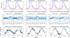 |
Fig. A.1 Input data and VAE reconstructions for three Gaia DR3 sources belonging to the ACV, β Cep, and SPB classes, respectively. The description of the rows and columns follows that of Fig. 1. |
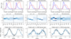 |
Fig. A.2 Input data and VAE reconstructions for three Gaia DR3 sources belonging to the δ Cep, δ Sct, and γ Dor star classes, respectively. The description of the rows and columns follows that of Fig. 1. |
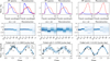 |
Fig. A.3 Input data and VAE reconstructions for three Gaia DR3 sources belonging to the AGN, CV, and YSO classes, respectively. The description of the rows and columns follows that of Fig. 1. |
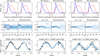 |
Fig. A.4 Input data and VAE reconstructions for three Gaia DR3 sources belonging to the RS, ELL, and SOLAR classes, respectively. The description of the rows and columns follows that of Fig. 1. |
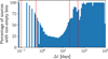 |
Fig. A.5 Percentage of sources with at least one pair of observations whose time difference falls in a given Δt bin. For each source the time differences are extracted and then binned in 100 equally spaced logarithmic bins. The structure is a result of Gaia’s sampling. The red dashed lines mark the edges of the low-resolution Δt bins used in this work. All sources have at least one observation in each of these low-resolution bins. |
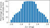 |
Fig. A.6 Percentage of sources with at least one pair of observations whose magnitude difference falls in a given Δm bin. The normalisation applied to the light curves ensures that the Δm distribution is centred around zero. |
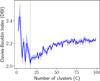 |
Fig. A.7 Davies-Bouldin index as a function of the number of clusters (lower is better). The minimum (C=17) is marked with a black dashed line. |
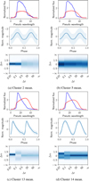 |
Fig. A.8 XP spectra, folded time series, and Δm|Δt reconstructed from the centroid (mean) of the clusters using the decoder of the VAEs. |
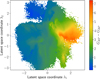 |
Fig. A.9 The distribution of the (potentially reddened) mean colour GBP − GRP in the latent space. |
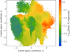 |
Fig. A.10 Distribution of the standard deviation of the observed Gaia G magnitude in the latent space. |
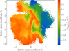 |
Fig. A.11 Distribution of the main frequency f1. |
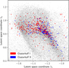 |
Fig. A.12 Region of the latent space containing the RR Lyr ab variables. The sample of RR Lyr stars plotted to show the Oosterhoff classification was taken from Prudil et al. (2019). |
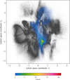 |
Fig. A.13 Location of Gaia DR3 sources with significant scan-angle dependent signal that induces a spurious variability signal. The sample was taken from Holl et al. (2023) with thresholds spearman_corr_ipd_g_fov > 0.9 and scan_angle_model_ampl_sig_g_fov > 10. |
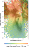 |
Fig. A.14 Same as Fig. 18, but colour represents the duration of the primary eclipse expressed as the fraction of the phase. |
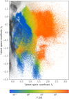 |
Fig. A.15 Same as for Fig. 19, but the Lomb-Scargle dominant period P1 is used for the colour coding. |
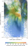 |
Fig. A.16 Same as Fig. 18, but colour represents the amplitude of the ellipsoidal variation (if any) in millimagnitude (mmag). |
Appendix B Neural network architecture details
The architecture of the encoder of the VAE for sampled XP low-resolution mean spectra is described as follows:
An FC layer with 110 inputs and 128 outputs, followed by layer normalisation (LN) and a GELU activation function.
An FC layer with 128 inputs and 128 outputs with LN and GELU activation.
An FC layer with 128 inputs and 2K outputs. The output is then split into two K arrays.
The output of the last layer represents the mean and the logarithm of the standard deviation, from which the latent variable is sampled using Eq. (5). After this, the data is reconstructed by a decoder ANN with the following architecture:
An FC layer with K inputs and 128 outputs with LN and GELU activation.
An FC layer with 128 inputs and 128 outputs with LN and GELU activation.
An FC layer with 128 inputs and 110 outputs with a ReLU activation to ensure non-negativity.
The log of the variance of the reconstructed spectra log ![Mathematical equation: $\[\sigma_{\text {XP }}^{2}\]$](/articles/aa/full_html/2025/09/aa54025-25/aa54025-25-eq39.png) , is predicted from the latent variables using a smaller network with the following architecture:
, is predicted from the latent variables using a smaller network with the following architecture:
An FC layer with K inputs and 128 outputs with LN and GELU activation.
An FC layer with 128 inputs and 1 output.
The Δm|Δt representation is compressed using an encoder composed of FC layers. The architecture is described as follows:
An FC layer with 115 (23 × 5) inputs and 128 outputs, followed by LN and a GELU activation function.
An FC layer with 128 inputs and 128 outputs with LN and GELU activation.
An FC layer with 128 inputs and 128 outputs with LN and GELU activation.
An FC layer with 128 inputs and 2K outputs. The output is then split into two K arrays.
The latent variables are sampled using Eq. (5) and given as input to a decoder with the following architecture:
An FC layer with K inputs and 128 outputs with LN and GELU activation.
An FC layer with 128 inputs and 128 outputs with LN and GELU activation.
An FC layer with 128 inputs and 128 outputs with LN and GELU activation.
An FC layer with 128 inputs and 115 outputs. The output is then reshaped into a 23 × 5 matrix and followed by a Softmax activation function to ensure that all values are non-negative and that they add up to one column-wise.
The architecture of the VAE for the folded Gaia G band light curves is described as follows:
The dimensionality of the phases ϕj is expanded using trigonometric functions as
![Mathematical equation: $\[\left[\cos \left(2 \pi h \phi_{j}\right), ~\sin \left(2 \pi h \phi_{j}\right)\right]_{h=1}^{H} \in \mathbb{R}^{2 H}\]$](/articles/aa/full_html/2025/09/aa54025-25/aa54025-25-eq40.png) and concatenated with the magnitudes forming an real-valued array E1 with dimensionality L × (1 + 2H).
and concatenated with the magnitudes forming an real-valued array E1 with dimensionality L × (1 + 2H).A GRU6 with input size (1 + 2H), hidden state size of 128 and dropout probability of 0.2, receives E1 and produces a real-valued array E2 with dimensionality L × 128.
A second GRU with input and hidden state size of 128, receives E2 and produces a real-valued array E3 with dimensionality L × 128.
An FC layer with 128 inputs and 1 output is used to obtain an attention score A = exp(FC(E3)) ∈ ℝL (Bahdanau et al. 2014). The score is multiplied by the binary mask B to set the attention of padded values to zero. Then, the attention scores are normalised so that they add to unity. We note that this is equivalent to applying the Softmax activation function to the attention scores, but compensating for the masked values. The normalised scores are used as weights to generate E4, a 128-dimensional vector that is the weighted average of E3 along the sequence dimension.
An FC layer with 128 inputs and 2K outputs reduces the dimensionality of E4. The output is then split into two K-dimensional arrays.
After sampling from the parameters using Eq. (5), the latent variable and the phases are given as input to the decoder. The architecture uses FC layers and is described as follows:
The phases are expanded using the same procedure described for the encoder, and concatenated with the latent variables forming an array D1 with dimensionality L × (K + 2H).
An FC layer with K + 2H inputs and 128 outputs with LN and GELU activation transforms D1 into D2.
An FC layer with 128 inputs and 128 outputs, with LN and GELU activation, transforms D2 into D3.
An FC layer with 128 inputs and 1 output transforms D3 into D4 ∈ ℝL. This corresponds to the reconstructed magnitudes.
During training, the phases given to the decoder have to match the ones used to encode the latent variables. However, at inference time, the decoder can reconstruct into a finer phase grid for visualisation purposes. This can be seen in the last row of Fig. 1. The architecture of the VAE to build the 2D representation that combines the latent variables from previous VAEs is described as follows:
An FC layer with 3K + 3 inputs and 128 outputs, followed by LN and a hyperbolic tangent (tanh) activation function.
An FC layer with 128 inputs and 128 outputs with LN and tanh activation.
An FC layer with 128 inputs and 4 outputs. The output is then split into two arrays with two variables each, corresponding to the mean and standard deviation of the latent variables.
The latent variables are sampled using Eq. (5) and given as input to a decoder ANN with the following architecture:
An FC layer with 2 inputs and 128 outputs with LN and tanh activation.
An FC layer with 128 inputs and 128 outputs with LN and tanh activation.
An FC layer with 128 inputs and 3K + 3 outputs.
References
- Abdurro’uf, Accetta, K., Aerts, C., et al. 2022, ApJS, 259, 35 [NASA ADS] [CrossRef] [Google Scholar]
- Aerts, C. 2021, Rev. Mod. Phys., 93, 015001 [Google Scholar]
- Aerts, C., & Tkachenko, A. 2024, A&A, 692, R1 [NASA ADS] [CrossRef] [EDP Sciences] [Google Scholar]
- Bahdanau, D., Cho, K., & Bengio, Y. 2014, in International Conference on Learning Representations 2015 [arXiv:1409.0473] [Google Scholar]
- Bellm, E. C., Kulkarni, S. R., Graham, M. J., et al. 2019, PASP, 131, 018002 [Google Scholar]
- Bengio, Y., Courville, A., & Vincent, P. 2013, IEEE Trans. Pattern Anal. Mach. Intell., 35, 1798 [CrossRef] [Google Scholar]
- Blagorodnova, N., Neill, J. D., Walters, R., et al. 2018, PASP, 130, 035003 [Google Scholar]
- Blažko, S. 1907, Astron. Nachr., 175, 325 [Google Scholar]
- Breiman, L. 2001, Mach. Learn., 45, 5 [Google Scholar]
- Breunig, M. M., Kriegel, H.-P., Ng, R. T., & Sander, J. 2000, SIGMOD Rec., 29, 93 [Google Scholar]
- Briquet, M., Hubrig, S., De Cat, P., et al. 2007, A&A, 466, 269 [NASA ADS] [CrossRef] [EDP Sciences] [Google Scholar]
- Buck, T., & Schwarz, C. 2024, in NIPS 2024 Workshop on Machine Learning and the Physical Sciences [arXiv:2410.16081] [Google Scholar]
- Burgess, C. P., Higgins, I., Pal, A., et al. 2018, in NIPS 2017 Workshop on Learning Disentangled Representations [arXiv:1804.03599] [Google Scholar]
- Carrasco, J. M., Weiler, M., Jordi, C., et al. 2021, A&A, 652, A86 [NASA ADS] [CrossRef] [EDP Sciences] [Google Scholar]
- Carnerero, M. I., Raiteri, C. M., Rimoldini, L., et al. 2023, A&A, 674, A24 [NASA ADS] [CrossRef] [EDP Sciences] [Google Scholar]
- Catelan, M. 2009, Ap&SS, 320, 261 [Google Scholar]
- Catelan, M., & Smith, H. A. 2015, Pulsating Stars (John Wiley & Sons) [Google Scholar]
- Chen, T., & Guestrin, C. 2016, in Proceedings of the 22nd ACM SIGKDD International Conference on Knowledge Discovery and Data Mining, KDD’16, 785 [Google Scholar]
- Chung, J., Gulcehre, C., Cho, K., & Bengio, Y. 2014, in NIPS 2014 Deep Learning and Representation Learning Workshop [arXiv:1412.3555] [Google Scholar]
- Clementini, G., Ripepi, V., Garofalo, A., et al. 2023, A&A, 674, A18 [NASA ADS] [CrossRef] [EDP Sciences] [Google Scholar]
- Cui, X.-Q., Zhao, Y.-H., Chu, Y.-Q., et al. 2012, Res. Astron. Astrophys., 12, 1197 [Google Scholar]
- Davies, D. L., & Bouldin, D. W. 1979, IEEE Trans. Pattern Anal. Mach. Intell., PAMI-1, 224 [Google Scholar]
- De Angeli, F., Weiler, M., Montegriffo, P., et al. 2023, A&A, 674, A2 [NASA ADS] [CrossRef] [EDP Sciences] [Google Scholar]
- DESI Collaboration (Adame, A. G., et al.) 2024, AJ, 168, 58 [NASA ADS] [CrossRef] [Google Scholar]
- Donoso-Oliva, C., Becker, I., Protopapas, P., et al. 2023, A&A, 670, A54 [NASA ADS] [CrossRef] [EDP Sciences] [Google Scholar]
- Evans, D. W., Eyer, L., Busso, G., et al. 2023, A&A, 674, A4 [NASA ADS] [CrossRef] [EDP Sciences] [Google Scholar]
- Eyer, L., & Mowlavi, N. 2008, in Journal of Physics Conference Series, 118, 012010 [Google Scholar]
- Eyer, L., Audard, M., Holl, B., et al. 2023, A&A, 674, A13 [NASA ADS] [CrossRef] [EDP Sciences] [Google Scholar]
- Falcon, W., Borovec, J., Wälchli, A., et al. 2020, https://zenodo.org/record/3828935 [Google Scholar]
- Fritzewski, D. J., Vanrespaille, M., Aerts, C., et al. 2025, A&A, 698, A253 [NASA ADS] [CrossRef] [EDP Sciences] [Google Scholar]
- Gaia Collaboration (Prusti, T., et al.) 2016, A&A, 595, A1 [NASA ADS] [CrossRef] [EDP Sciences] [Google Scholar]
- Gaia Collaboration (De Ridder, J., et al.) 2023a, A&A, 674, A36 [CrossRef] [EDP Sciences] [Google Scholar]
- Gaia Collaboration (Vallenari, A., et al.) 2023b, A&A, 674, A1 [NASA ADS] [CrossRef] [EDP Sciences] [Google Scholar]
- Garrison, L. H., Foreman-Mackey, D., Shih, Y.-h., & Barnett, A. 2024, RNAAS, 8, 250 [Google Scholar]
- Gavras, P., Rimoldini, L., Nienartowicz, K., et al. 2023, A&A, 674, A22 [NASA ADS] [CrossRef] [EDP Sciences] [Google Scholar]
- Ginsburg, A., Sipőcz, B. M., Brasseur, C. E., et al. 2019, AJ, 157, 98 [Google Scholar]
- Glorot, X., Bordes, A., & Bengio, Y. 2011, in Proceedings of Machine Learning Research, 15, Proceedings of the Fourteenth International Conference on Artificial Intelligence and Statistics (PMLR), 315 [Google Scholar]
- Goodfellow, I., Bengio, Y., & Courville, A. 2016, Deep Learning (The MIT Press) [Google Scholar]
- Gui, J., Chen, T., Zhang, J., et al. 2024, IEEE Trans. Pattern Anal. Mach. Intell., 46, 9052 [Google Scholar]
- Guiglion, G., Nepal, S., Chiappini, C., et al. 2024, A&A, 682, A9 [NASA ADS] [CrossRef] [EDP Sciences] [Google Scholar]
- Guo, W., Wang, J., & Wang, S. 2019, IEEE Access, 7, 63373 [CrossRef] [Google Scholar]
- He, K., Zhang, X., Ren, S., & Sun, J. 2015, in Proceedings of the IEEE International Conference on Computer Vision (ICCV), IEEE, 1026 [Google Scholar]
- Heinze, A. N., Tonry, J. L., Denneau, L., et al. 2018, AJ, 156, 241 [Google Scholar]
- Hendrycks, D., & Gimpel, K. 2016, arXiv e-prints [arXiv:1606.08415] [Google Scholar]
- Hey, D., & Aerts, C. 2024, A&A, 688, A93 [NASA ADS] [CrossRef] [EDP Sciences] [Google Scholar]
- Hochreiter, S., Schmidhuber, J., & Elvezia, C. 1997, Neural Computat., 9, 1735 [Google Scholar]
- Holl, B., Fabricius, C., Portell, J., et al. 2023, A&A, 674, A25 [NASA ADS] [CrossRef] [EDP Sciences] [Google Scholar]
- Hu, W., & Tan, Y. 2018, in AAAI Workshops, 245 [Google Scholar]
- Huertas-Company, M., Sarmiento, R., & Knapen, J. H. 2023, RAS Tech. Instrum., 2, 441 [NASA ADS] [CrossRef] [Google Scholar]
- Jamal, S., & Bloom, J. S. 2020, ApJS, 250, 30 [NASA ADS] [CrossRef] [Google Scholar]
- Jayasinghe, T., Stanek, K. Z., Kochanek, C. S., et al. 2019, MNRAS, 486, 1907 [NASA ADS] [Google Scholar]
- Jiang, Z., Zheng, Y., Tan, H., Tang, B., & Zhou, H. 2017, in Proceedings of the 26th International Joint Conference on Artificial Intelligence, 1965 [Google Scholar]
- Kingma, D. P., & Ba, J. 2015, in International Conference on Learning Representations (ICLR) [arXiv:1412.6980] [Google Scholar]
- Kingma, D. P., & Welling, M. 2014, in International Conference on Learning Representations (ICLR) [arXiv:1312.6114] [Google Scholar]
- Laroche, A., & Speagle, J. S. 2023, in International Conference in Machine Learning, Workshop on Machine Learning for Astrophysics [arXiv:2307.06378] [Google Scholar]
- Lebzelter, T., Mowlavi, N., Lecoeur-Taibi, I., et al. 2023, A&A, 674, A15 [NASA ADS] [CrossRef] [EDP Sciences] [Google Scholar]
- Lei Ba, J., Kiros, J. R., & Hinton, G. E. 2016, arXiv e-prints [arXiv:1607.06450] [Google Scholar]
- Liu, X., Zhang, F., Hou, Z., et al. 2021, IEEE Trans. Knowledge Data Eng., 35, 857 [Google Scholar]
- Lomb, N. R. 1976, Ap&SS, 39, 447 [Google Scholar]
- Luongo, E., Ripepi, V., Marconi, M., et al. 2024, A&A, 690, L17 [NASA ADS] [CrossRef] [EDP Sciences] [Google Scholar]
- Mahabal, A., Sheth, K., Gieseke, F., et al. 2017, in 2017 IEEE symposium Series on Computational Intelligence (SSCI), IEEE, 1 [Google Scholar]
- Martínez-Palomera, J., Bloom, J. S., & Abrahams, E. S. 2022, AJ, 164, 263 [CrossRef] [Google Scholar]
- Mombarg, J. S. G., Aerts, C., Van Reeth, T., & Hey, D. 2024, A&A, 691, A131 [NASA ADS] [CrossRef] [EDP Sciences] [Google Scholar]
- Mowlavi, N., Holl, B., Lecoeur-Taïbi, I., et al. 2023, A&A, 674, A16 [NASA ADS] [CrossRef] [EDP Sciences] [Google Scholar]
- Nair, V., & Hinton, G. E. 2010, in Proceedings of the 27th International Conference on Machine Learning (ICML-10), 807 [Google Scholar]
- Naul, B., Bloom, J. S., Pérez, F., & van der Walt, S. 2018, Nat. Astron., 2, 151 [NASA ADS] [CrossRef] [Google Scholar]
- Oosterhoff, P. T. 1939, The Observatory, 62, 104 [NASA ADS] [Google Scholar]
- Oosterhoff, P. T. 1944, Bull. Astron. Inst. Netherlands, 10, 55 [NASA ADS] [Google Scholar]
- Pang, G., Shen, C., Cao, L., & van den Hengel, A. 2021, ACM Comput. Surv., 54 [Google Scholar]
- Parker, L., Lanusse, F., Golkar, S., et al. 2024, MNRAS, 531, 4990 [Google Scholar]
- Paszke, A., Gross, S., Massa, F., et al. 2019, in Advances in Neural Information Processing Systems (NIPS), 32 (Curran Associates, Inc.), 8024 [Google Scholar]
- Pedregosa, F., Varoquaux, G., Gramfort, A., et al. 2011, J. Mach. Learn. Res., 12, 2825 [Google Scholar]
- Prudil, Z., Dékány, I., Catelan, M., et al. 2019, MNRAS, 484, 4833 [NASA ADS] [Google Scholar]
- Radford, A., Kim, J. W., Hallacy, C., et al. 2021, in International Conference on Machine Learning, PMLR, 8748 [Google Scholar]
- Rimoldini, L., Eyer, L., Audard, M., et al. 2022, Gaia DR3 documentation Chapter 10: Variability, Gaia DR3 documentation, European Space Agency; Gaia Data Processing and Analysis Consortium. Online at https://gea.esac.esa.int/archive/documentation/GDR3/index.html, 10 [Google Scholar]
- Rimoldini, L., Holl, B., Gavras, P., et al. 2023, A&A, 674, A14 [NASA ADS] [CrossRef] [EDP Sciences] [Google Scholar]
- Rizhko, M., & Bloom, J. S. 2025, AJ, 170, 28 [Google Scholar]
- Ruz-Mieres, D. 2024 https://doi.org/10.5281/zenodo.11617977 [Google Scholar]
- Sánchez-Sáez, P., Lira, H., Martí, L., et al. 2021, AJ, 162, 206 [CrossRef] [Google Scholar]
- Sartoretti, P., Marchal, O., Babusiaux, C., et al. 2023, A&A, 674, A6 [NASA ADS] [CrossRef] [EDP Sciences] [Google Scholar]
- Scargle, J. D. 1982, ApJ, 263, 835 [Google Scholar]
- Skarka, M., Prudil, Z., & Jurcsik, J. 2020, MNRAS, 494, 1237 [NASA ADS] [CrossRef] [Google Scholar]
- Smith, H. A. 1995, Cambr. Astrophys. Ser., 27 [Google Scholar]
- Soraisam, M. D., Saha, A., Matheson, T., et al. 2020, ApJ, 892, 112 [Google Scholar]
- The Multimodal Universe Collaboration (Audenaert, J., et al.) 2024, in The Thirty-eight Conference on Neural Information Processing Systems (NIPS) Datasets and Benchmarks Track [arXiv:2412.02527] [Google Scholar]
- Udalski, A., Szymanski, M. K., Soszynski, I., & Poleski, R. 2008, Acta Astron., 58, 69 [NASA ADS] [Google Scholar]
- Zhang, G., Helfer, T., Gagliano, A. T., Mishra-Sharma, S., & Ashley Villar, V. 2024, Mach. Learn. Sci. Technol., 5, 045069 [Google Scholar]
This flag is the result of the operators described in Section 10.2.3 of the Gaia DR3 documentation (Rimoldini et al. 2022).
Only 1.64% of the light curves in the dataset have more than 100 observations.
This quantity is removed during preprocessing and is therefore unavailable to the models.
Together, these four classes make less than 0.1% of the subset.
Preliminary experiments showed that the difference in performance between GRU and the more complex LSTM (Hochreiter et al. 1997) was negligible; hence, as the former is more efficient, it was preferred.
All Tables
Average computational time required to process a Gaia source with 100 observations. The GPU times were measured for a batch of size 256. Hardware: Intel Xeon 5117 CPU, NVIDIA A4000 GPU.
Supervised classification performance metrics per class using all latent variables as input.
All Figures
|
Fig. 1 Input data and VAE reconstructions for three variable Gaia DR3 sources. The sources shown in each column are associated with the RR Lyr ab star, ECLb, and LPV classes, respectively. Each row corresponds to a specific data modality and shows the preprocessed input data (prior to compression) and its reconstruction (after decompression) using the VAEs described in Sections 4.1, 4.2, and 4.3. The first row corresponds to the sampled representation of the Gaia BP (solid blue) and RP (dashed red) low-resolution spectra. The second row depicts the conditional distribution of magnitude differences given time differences of the Gaia G band light curves. The third row shows the Gaia G band light curve folded with its dominant period. |
| In the text | |
|
Fig. 2 Variational autoencoder used to create a K = 5 dimensional latent space given the 2 × 55 continuous BP and RP spectra points. Each coloured rectangle represents a layer of the ANN, with the size of the output vector given at the top. The encoder starts with the (standardised) observations denoted in the leftmost white rectangle, and ends with the K = 5-dimensional latent space denoted in green, representing the position μ and its (spherical) uncertainty σ2 of the observed data in the latent space. The decoder starts by sampling a K=5-dimensional value z from a Gaussian distribution with mean μ and the diagonal covariance matrix σ2, and ends with the reconstructed 2 × 55 XP spectra values. Some layers use ‘layer normalisation’, which is denoted by LN. The activation function of the neurons in a particular layer is noted at the bottom: GELU, LIN (linear), or ReLU. |
| In the text | |
|
Fig. 3 Variational autoencoder used to create a K=5 dimensional latent space given the 23 × 5 values of the observed Δm|Δt histogram. The explanation of the network is very similar to the one in Fig. 2. |
| In the text | |
|
Fig. 4 Variational autoencoder used to create a K = 5 dimensional latent space given the 100 points of the folded light curve (phase ϕj ∈ [0, 1] and the standardised G-magnitude mj). The network does not receive the 100 phase values ϕj directly but rather the 100 × H values sin(2πhϕj), with h = 1, . . ., H and an equal number of values cos(2πhϕj). The first neural layer is a GRU to which the observations are fed sequentially (SEQ), i.e. 100 consecutive sets of size 1 + 2H corresponding to each time point of the light curve. The result is a matrix of size 100 × 128. Each of the 100 rows is then fed sequentially to the next GRU layer, resulting in a matrix of the same shape. The next layer takes each row of this matrix (of size 128), and computes an attention score corresponding to each point of the light curve. These scores are then used in a subsequent layer to compute a weighted average over the matrix rows, producing a feature set of size 128 where the time points that were deemed more important given the attention score receive a higher weight. In the final layers of the encoder, this feature set is then further reduced to the K = 5-dimensional latent coordinates (purple rectangles). The decoder works similarly as explained in Fig. 2, but now also receives the phase information (sin(2πhϕj), cos(2πhϕj)). The first decoding neural layer results in a matrix of size 100 × 128. Each row (of size 128) of this matrix is then fed to a neural layer, resulting again in a 100 × 128 matrix, which is then further reduced to a vector of size 100 by the final decoding layer, resulting in the 100 reconstructed (standardised) magnitudes of the folded light curve. |
| In the text | |
|
Fig. 5 Variational autoencoder used to further reduce the latent spaces produced by the networks illustrated in Figs. 2–4 (the green, orange, and purple rectangles) to a latent space of dimension 2, providing the coordinates (λ1, λ2) that are used for the interpretation in Section 9. Apart from the location in the 3K = 15-dimensional latent space, the VAE also receives the standard deviation of the G light curve, the colour estimate |
| In the text | |
|
Fig. 6 Gaia DR3 source 4037765863920151040 XP mean spectra corresponding to a long period variable (first column). These data were compressed using the VAE and then reconstructed. The following columns show the reconstruction and the squared difference between the original and its reconstruction as the number of latent variables, K, increases. |
| In the text | |
|
Fig. 7 Folded G band light curve of Gaia source DR3 5410617628478565248 corresponding to an eclipsing binary (first column). These data were compressed using the VAE and then reconstructed. The following columns show the reconstruction and the squared difference between the original as K increases. |
| In the text | |
|
Fig. 8 Average ELBO (in blue) and macro F1−score (in red) in the validation set as a function of the number of latent variables (K). Higher is better for both metrics. A black dashed line marks K = 5. |
| In the text | |
|
Fig. 9 Local outlier factor vs the variance of the G band folded light curve decoder ( |
| In the text | |
|
Fig. 10 Folded light curves (black dots) and their reconstructions (blue) for the three sources in the RR Lyr SOS table with highest LOF (left panels) and highest |
| In the text | |
|
Fig. 11 Confusion matrices for the test partition sources of the labelled subset. The rows correspond to the ground truth class selected from Gavras et al. (2023), and the columns to the class predicted by the classifier using the latent variables as input. The cell in the i-th row and j-th column gives the percentage of sources labelled as class i and predicted as class j with respect to the total number of sources of class i. Each matrix represents the averaged results of a linear classifier trained on different sets of latent variables. Standard deviations are shown after the | symbol. Percentage rates and corresponding standard deviations below 1% are not shown for clarity. |
| In the text | |
|
Fig. 12 Clustering results of the latent variables organised into 17 groups using k-means (top panel) and a Gaussian mixture model with full covariance (bottom panel). Rows show the distribution of the classes across the clusters (rows add up to 100). Red lines highlight the class that constitutes the majority within each cluster. |
| In the text | |
|
Fig. 13 Distribution of the 4 136 544 sources in the 2 D latent output space of our ANN designed to perform an unsupervised clustering of variable sources (see Section 4 and Fig. 5 for more details). Different overdensities of points correspond to different (sub)types of variability. A first identification of the overdensities can be found in Fig. 14. For future reference we also depict the parts of this latent space shown in Figs. 15–20 with rectangles and provide the figure number is in one of the corners. |
| In the text | |
|
Fig. 14 Most frequently occurring variability class for each bin of the latent space shown in Fig. 13 for the set of variable stars that have a variability class label available (see Section 3). The bins are colour-coded with the fraction of stars in the bin that have the shown label. Only the variability classes SPB, γ Dor, β Cep, δ Sct, CP stars, AGNs, LPVs, RR Lyr (ab, c, and d), Cepheids, WDs, eclipsing binaries (EA, EB, EW), ELL variables, Be (BE) variables, and YSO variables were taken into account to generate this figure. |
| In the text | |
|
Fig. 15 Region of the latent space where the RR Lyr stars are located. The RR Lyr variables for which a “RRab” classification label was available in the Gaia DR3 catalogue are overplotted in colour, where we used the pulsation amplitude A11 for the colour scale. The RR Lyr c and RR Lyr d variables are plotted in blue resp. red. |
| In the text | |
|
Fig. 16 Sources for which we have a γ Dor or a white dwarf classification label from the literature are shown in red and orange, respectively. For the known δ Sct variables, we used a colour scheme that shows the standard deviation in the Gaia G passband as a proxy for the oscillation amplitude. We indicate the position of the high-amplitude δ Sct stars (HADS), with amplitude above 100 mmag. |
| In the text | |
|
Fig. 17 Region of the latent space where the variable B stars are projected. The β Cep, SPB, and CP variables for which we have a classification from the DPAC-CU7 training set mentioned in Section 3 are plotted in colour. |
| In the text | |
|
Fig. 18 Part of the latent space where the ANN projects eclipsing and ellipsoidal binaries. The grey background shows the same density as in Fig. 13. Sources that were published in the Gaia DR3 Variability catalogue gaiadr3.vari_eclipsing_binary are overplotted in a 2D histogram of small hexagons where the colour of each hexagon corresponds to the average magnitude difference between primary and secondary eclipses of the sources inside that bin. |
| In the text | |
|
Fig. 19 Part of the latent space where the ANN projects the long period variables. The grey background shows the same density as in Fig. 13. In colour, we overplotted the sources which were published in the Gaia DR3 Variability catalogue as a candidate O-rich or C-type LPVs. The quantity ⟨Δλ⟩RP was taken from the same catalogue (column name median_delta_wl_rp) and probes particular molecular bands in the RP spectrum (see text). |
| In the text | |
|
Fig. 20 Region of the latent space occupied by AGNs. For the AGN candidates published in the Gaia DR3 release, we colour-coded the frequency with the highest amplitude found in the Lomb-Scargle frequencygram computed from the light curves in the Gaia G passband. |
| In the text | |
|
Fig. A.1 Input data and VAE reconstructions for three Gaia DR3 sources belonging to the ACV, β Cep, and SPB classes, respectively. The description of the rows and columns follows that of Fig. 1. |
| In the text | |
|
Fig. A.2 Input data and VAE reconstructions for three Gaia DR3 sources belonging to the δ Cep, δ Sct, and γ Dor star classes, respectively. The description of the rows and columns follows that of Fig. 1. |
| In the text | |
|
Fig. A.3 Input data and VAE reconstructions for three Gaia DR3 sources belonging to the AGN, CV, and YSO classes, respectively. The description of the rows and columns follows that of Fig. 1. |
| In the text | |
|
Fig. A.4 Input data and VAE reconstructions for three Gaia DR3 sources belonging to the RS, ELL, and SOLAR classes, respectively. The description of the rows and columns follows that of Fig. 1. |
| In the text | |
|
Fig. A.5 Percentage of sources with at least one pair of observations whose time difference falls in a given Δt bin. For each source the time differences are extracted and then binned in 100 equally spaced logarithmic bins. The structure is a result of Gaia’s sampling. The red dashed lines mark the edges of the low-resolution Δt bins used in this work. All sources have at least one observation in each of these low-resolution bins. |
| In the text | |
|
Fig. A.6 Percentage of sources with at least one pair of observations whose magnitude difference falls in a given Δm bin. The normalisation applied to the light curves ensures that the Δm distribution is centred around zero. |
| In the text | |
|
Fig. A.7 Davies-Bouldin index as a function of the number of clusters (lower is better). The minimum (C=17) is marked with a black dashed line. |
| In the text | |
|
Fig. A.8 XP spectra, folded time series, and Δm|Δt reconstructed from the centroid (mean) of the clusters using the decoder of the VAEs. |
| In the text | |
|
Fig. A.9 The distribution of the (potentially reddened) mean colour GBP − GRP in the latent space. |
| In the text | |
|
Fig. A.10 Distribution of the standard deviation of the observed Gaia G magnitude in the latent space. |
| In the text | |
|
Fig. A.11 Distribution of the main frequency f1. |
| In the text | |
|
Fig. A.12 Region of the latent space containing the RR Lyr ab variables. The sample of RR Lyr stars plotted to show the Oosterhoff classification was taken from Prudil et al. (2019). |
| In the text | |
|
Fig. A.13 Location of Gaia DR3 sources with significant scan-angle dependent signal that induces a spurious variability signal. The sample was taken from Holl et al. (2023) with thresholds spearman_corr_ipd_g_fov > 0.9 and scan_angle_model_ampl_sig_g_fov > 10. |
| In the text | |
|
Fig. A.14 Same as Fig. 18, but colour represents the duration of the primary eclipse expressed as the fraction of the phase. |
| In the text | |
|
Fig. A.15 Same as for Fig. 19, but the Lomb-Scargle dominant period P1 is used for the colour coding. |
| In the text | |
|
Fig. A.16 Same as Fig. 18, but colour represents the amplitude of the ellipsoidal variation (if any) in millimagnitude (mmag). |
| In the text | |
Current usage metrics show cumulative count of Article Views (full-text article views including HTML views, PDF and ePub downloads, according to the available data) and Abstracts Views on Vision4Press platform.
Data correspond to usage on the plateform after 2015. The current usage metrics is available 48-96 hours after online publication and is updated daily on week days.
Initial download of the metrics may take a while.