| Issue |
A&A
Volume 702, October 2025
|
|
|---|---|---|
| Article Number | A66 | |
| Number of page(s) | 30 | |
| Section | Extragalactic astronomy | |
| DOI | https://doi.org/10.1051/0004-6361/202554473 | |
| Published online | 08 October 2025 | |
The SWAN view of dense gas in the Whirlpool
A cloud-scale comparison of N2H+, HCO+, HNC, and HCN emission in M51
1
Max-Planck-Institut für Astronomie, Königstuhl 17, 69117 Heidelberg, Germany
2
Fakultät für Physik und Astronomie, Universität Heidelberg, Im Neuenheimer Feld 226, 69120 Heidelberg, Germany
3
Observatorio Astronómico Nacional (IGN), C/ Alfonso XII, 3, E-28014 Madrid, Spain
4
Argelander-Institut für Astronomie, Universität Bonn, Auf dem Hügel 71, 53121 Bonn, Germany
5
Center for Astrophysics | Harvard & Smithsonian, 60 Garden St., 02138 Cambridge, MA, USA
6
IRAM, 300 rue de la Piscine, F-38406 Saint Martin d’Hères, France
7
LUX, Observatoire de Paris, PSL Research University, CNRS, Sorbonne Universités, 75014 Paris, France
8
European Southern Observatory, Karl-Schwarzschild 2, 85748 Garching bei Muenchen, Germany
9
AURA for ESA, Space Telescope Science Institute, 3700 San Martin Drive, Baltimore, MD 21218, USA
10
Department of Astrophysical Sciences, Princeton University, 4 Ivy Lane, Princeton, NJ 08544, USA
11
Max-Planck-Institut für extraterrestrische Physik, Giessenbachstraße 1, D-85748 Garching, Germany
12
Department of Physics & Astronomy, University of Wyoming, Laramie, WY 82071, USA
13
National Radio Astronomy Observatory, 520 Edgemont Road, Charlottesville, VA 22903, USA
14
Universität Heidelberg, Zentrum für Astronomie, Institut für Theoretische Astrophysik, Albert-Ueberle-Str. 2, 69120 Heidelberg, Germany
15
Research School of Astronomy and Astrophysics, Australian National University, Canberra, ACT 2611, Australia
16
Universität Heidelberg, Interdisziplinäres Zentrum für Wissenschaftliches Rechnen, Im Neuenheimer Feld 225, 69120 Heidelberg, Germany
17
Radcliffe Institute for Advanced Study, Harvard University, 10 Garden St, 02138 Cambridge, MA, USA
18
Purple Mountain Observatory, Chinese Academy of Sciences, 10 Yuanhua Road, Nanjing 210023, China
19
Sterrenkundig Observatorium, Universiteit Gent, Krijgslaan 281 S9, B-9000 Gent, Belgium
20
Department of Physics, Tamkang University, No.151, Yingzhuan Road, Tamsui District, New Taipei City 251301, Taiwan
21
Faculty of Global Interdisciplinary Science and Innovation, Shizuoka University, 836 Ohya, Suruga-ku, Shizuoka 422-8529, Japan
22
Sub-department of Astrophysics, Department of Physics, University of Oxford, Keble Road, Oxford OX1 3RH, UK
⋆ Corresponding author.
Received:
11
March
2025
Accepted:
18
July
2025
Abstract
Tracing dense molecular gas, the fuel for star formation, is essential for understanding the evolution of molecular clouds and star-formation processes. We compared the emission of HCN (1–0), HNC (1–0), and HCO+(1–0) with the emission of N2H+(1–0) at cloud scales (125 pc) across the central 5 × 7 kpc of the Whirlpool galaxy, M51a, from “Surveying the Whirlpool galaxy at Arcseconds with NOEMA” (SWAN). We find that the integrated intensities of HCN, HNC, and HCO+ are more steeply correlated with N2H+ emission compared to the bulk molecular gas tracer CO, and we find variations in this relation across the center, molecular ring, northern, and southern disk of M51. Compared to HCN and HNC emission, the HCO+ emission follows the N2H+ emission more closely across the environments and physical conditions, such as the surface densities of molecular gas, stellar mass, star-formation rate, dynamical equilibrium pressure, and radius. Under the assumption that N2H+ is a fair tracer of dense gas at these scales, this makes HCO+ a more favorable dense gas tracer than HCN within the inner disk of M51. In all environments within our field of view, even when the central 2 kpc are removed, the ratio HCN/CO, which is commonly used to trace average cloud density, is only weakly dependent on molecular gas mass surface density. While ratios of other dense gas lines to CO show a steeper dependence on the surface density of molecular gas, this relation is still shallow in comparison to other nearby star-forming disk galaxies. One reason might be physical conditions in M51, which are different from other normal star-forming galaxies. Increased ionization rates, increased dynamical equilibrium pressure in the central few kiloparsecs, and the impact of the dwarf companion galaxy NGC 5195 are proposed mechanisms that might enhance HCN and HNC emission over HCO+ and N2H+ emission at larger-scale environments and cloud scales.
Key words: ISM: molecules / galaxies: ISM / galaxies: individual: M51
NASA Hubble Fellow.
Jansky Fellow of the National Radio Astronomy Observatory.
© The Authors 2025
 Open Access article, published by EDP Sciences, under the terms of the Creative Commons Attribution License (https://creativecommons.org/licenses/by/4.0), which permits unrestricted use, distribution, and reproduction in any medium, provided the original work is properly cited.
This article is published in open access under the Subscribe to Open model.
Open access funding provided by Max Planck Society.
1. Introduction
Star formation is one of the most fundamental processes in the Universe (see reviews by Krumholz 2014; Klessen et al. 2015; Schinnerer & Leroy 2024). As the birth of a star is ultimately linked to collapsing clouds of dense gas, the molecular gas phase is the key objective to study. Modern extragalactic observations (e.g., surveys such as the “Physics at high angular resolution in nearby galaxies” (PHANGS-ALMA); Leroy et al. 2021a,b) show that molecular clouds are linked sensitively to their galactic environment. As an example, a cloud’s velocity dispersion, surface density, and virial state all vary depending on whether the cloud is located in the main disk or near the center, in a spiral arm or interarm region, or in a stellar bar (Querejeta et al. 2019; Bešlic et al. 2021; Neumann et al. 2024). This implies that the host galaxy impacts the initial conditions for star formation. However, how exactly those changes in cloud properties translate into the global pattern of star formation is still unknown (see recent review by Schinnerer & Leroy 2024). As stars must form out of the densest gas in molecular clouds (Gao & Solomon 2004; Wu et al. 2005; Lada et al. 2012; Evans et al. 2014), two of the key open questions in astronomy are: (a) how to reliably access those densest molecular regions observationally and (b) how the properties of dense gas and therefore star formation is influenced by larger-scale environmental processes.
Line emission of molecules such as CO (1–0) is well suited for tracing the bulk molecular gas distribution in regions of high metallicity, such as local galaxy disks (e.g., Leroy et al. 2021b). In contrast to CO, the higher-dipole moment molecular species such as HCN, HNC, and HCO+ preferentially emit at higher physical densities. HCN has long been used to trace dense gas by the extragalactic community due to its relatively bright transition lines, which make it accessible in extragalactic targets (e.g., Helfer & Blitz 1993; Aalto et al. 1997, 2002; Gao & Solomon 2004; Meier & Turner 2005; Aalto et al. 2012; Bigiel et al. 2016; Jiménez-Donaire et al. 2019; Querejeta et al. 2019; Bemis & Wilson 2019; Krieger et al. 2020; Bešlic et al. 2021; Eibensteiner et al. 2022; Imanishi et al. 2023; Neumann et al. 2023a).
Still, at subcloud scales, studies from the Milky Way remain inconclusive about whether HCN only reliably traces the actual star-forming gas phase (e.g., Pety et al. 2017; Kauffmann et al. 2017; Mills & Battersby 2017; Barnes et al. 2020; Tafalla et al. 2021, 2023), as subthermal emission from low density regions can dominate the emission output in some of these cases. Furthermore, HCN emission can be excited by electrons in addition to collisional excitation by H2 molecules (Goldsmith & Kauffmann 2017) and, for example, Santa-Maria et al. (2023) showed that low visual extinction gas could amount to about 30% of the total HCN luminosity in Orion B. Recent numerical simulations of star-forming clouds in conditions similar to the local interstellar medium (ISM, e.g., Jones et al. 2023; Priestley et al. 2023, 2024) also suggest that a significant fraction of the HCN emission emanates from regions with densities of a few thousand cm−3 that are unlikely to form stars.
An improved approach to gauging the gas density is to contrast the emission of HCN with the emission of a bulk molecular gas tracer that emits preferentially at lower densities than HCN. This is a promising probe of the average physical cloud density as shown by simulations (Leroy et al. 2017a; Neumann et al. 2023a) and observations at ≳300 pc resolution in nearby galaxies (e.g., Neumann et al. 2023a, 2024; Schinnerer & Leroy 2024; Neumann et al. 2025).
An alternative to these lines is the molecular ion diazenylium (N2H+), which is a tracer of dense gas for chemical reasons. Within the Milky Way, N2H+(1–0) seems to be exclusively detected in dense and cold regions (H2 column densities above 1022 cm−2; Pety et al. 2017; Kauffmann et al. 2017; Tafalla et al. 2021). At these column densities, CO molecules start to freeze to dust grains in the coldest and densest parts of clouds. This allows N2H+ molecules to thrive as reactions of N2H+ and CO and H3+ and CO are inhibited, which is the main destruction mechanism of N2H+ and the main mechanism that limits the formation of N2H+ out of H3+. After the onset of star formation, stellar feedback heats the dust and evaporates the CO molecules, which increases the destruction of N2H+. This makes N2H+ molecules only selective for certain cold and high density regimes (i.e., Tafalla et al. 2023; Barnes et al. 2020). Hydrodynamical simulations show that, in contrast to HCN, HNC, and HCO+, N2H+ exists mostly in regions dense enough that they irreversibly undergo gravitational collapse (Priestley et al. 2023).
To understand the interplay between larger-scale dynamical features in galaxies and star formation, it is crucial to observe and study the properties of dense gas not just in individual clouds but across entire ensembles of clouds within different environments, which makes local galaxies the ideal testbeds to study dense gas. Since N2H+(1–0) emission is several order of magnitude fainter than 12CO(1–0) (Schinnerer & Leroy 2024), and several times fainter than HCN (1–0) emission (Jiménez-Donaire et al. 2023), extragalactic observations of N2H+ have so far been limited to either larger-scale lower-resolution studies (i.e., kiloparsec-scales, Sage & Ziurys 1995; den Brok et al. 2022; Jiménez-Donaire et al. 2023), or higher-resolution studies of individual regions such as starburst galaxy centers (e.g., the centers of NGC 253, IC342, and NGC 6946; Martín et al. 2021; Meier & Turner 2005; Eibensteiner et al. 2022).
Surveying the Whirlpool galaxy at Arcseconds with NOEMA (SWAN), a Large Program of the IRAM Northern Extended Millimetre Array (NOEMA) and IRAM-30m telescope, therefore represents the next logical step in understanding dense molecular gas. SWAN (Stuber et al. 2025) is a high-resolution (125 pc), high-sensitivity survey that maps the emission of several 3 mm lines, including the J = 1–0 transition of so-called dense gas tracers HCN, HNC, HCO+, and N2H+ across the central ∼5 × 7 kpc2 of the Whirlpool galaxy (NGC 5194 or M51a). As the fraction of dense gas (as traced by HCN) is found to vary drastically with galaxy environment at both kiloparsec and cloud-scale resolutions (Usero et al. 2015; Gallagher et al. 2018; Jiménez-Donaire et al. 2019; Querejeta et al. 2019; Bemis & Wilson 2019; Bešlic et al. 2021; Neumann et al. 2023a), it is vital to reliably study the denser molecular gas phase across different environments. With the SWAN survey, for the first time we can access not only the common dense gas tracer HCN, but also the chemical tracer N2H+ at an unprecedented resolution in M51 across the inner spiral arms and interarm regions, molecular ring, nuclear bar, and center with known active galactic nucleus (AGN) and outflow (Ho et al. 1997; Dumas et al. 2011; Querejeta et al. 2016a). M51a, also known as the Whirlpool galaxy or NGC 5194 (M51 hereafter), is a massive star-forming galaxy in the northern hemisphere, known for its iconic grand-design spiral arm structure, high surface brightness, low inclination, and proximity. Many molecular line studies have targeted M51 in the past (Koda et al. 2011; Schinnerer et al. 2013; Watanabe et al. 2014; Chen et al. 2017; Querejeta et al. 2019; den Brok et al. 2022) and its complex dynamics, partially triggered by interactions with the dwarf galaxy M51b, are well studied (Meidt et al. 2013; Colombo et al. 2014a; Querejeta et al. 2016a). We list the main properties of M51 in Table 1.
Overview of the main properties of M51 (NGC 5194).
In Stuber et al. (2023, S23 hereafter,) we presented the first high-resolution map of N2H+ across a larger-scale field of view (FoV) (5 × 7 kpc2) in an extragalactic target, M51. As the formation of stars is also closely connected with dense molecular clouds (Schinnerer & Leroy 2024), we further probe the impact of surface densities of SFR (ΣSFR) and stellar mass (Σ*) on the dense gas emission in this work. In addition, we test hypothesized links between dense gas mass, CO velocity dispersion (σCO), galactocentric radius, and dynamical equilibrium pressure (PDE). In a hydrostatic equilibrium, the midplane pressure, PDE, determines the ability of the ISM to form molecular gas, and is expected to rise with a cloud’s mean density (Jiménez-Donaire et al. 2019). At 125 pc scales, we found a superlinear correlation between N2H+(1–0) and HCN(1–0) when excluding the AGN-affected center in S23. Here, we expand this work to include the emission of the additional high-dipole molecules HNC and HCO+(1–0), and to study what sets the density distribution and cloud-scale chemistry across M51’s environments. We compare those emission lines to tracers of the surface density of molecular gas, as a proxy for the average gas density and other physical properties of the gas disk related to star formation.
Section 2 describes our observations and data reduction and Section 3 describes our methodology. In Section 4, we make a direct comparison of the molecular emission lines with each other and then consider how the emission compares to the bulk molecular gas tracer 12CO. We then probe the dependence of dense gas tracing molecular emission with various surface densities (Sect. 5). We discuss the chemical composition and environmental dependence of the quiescent and star-forming dense gas in Sect. 6 and summarize our results in Sect. 7.
2. Observations and data
To study the relation between galaxy environment and competing tracers of dense gas, we use the N2H+, HCN, HNC and HCO+ maps from the SWAN survey (Stuber et al. 2025, Sect. 2.1) that cover the AGN and outflow, nuclear bar, molecular ring and inner spiral arms and interarm region in M51a at cloud-scales. We combine 3 mm line emission observations with observations of bulk molecular gas tracer 12CO(1–0) from the PdBI Arcsecond Whirlpool Survey (PAWS, Schinnerer et al. 2013). To test the physical conditions driving changes in the emission of dense gas tracing lines, we obtain surface density maps of SFR (ΣSFR), molecular gas surface density (Σmol), stellar mass (Σ*), as well as estimate the dynamical equilibrium pressure (PDE) from ancillary data (Sect. 2.3). The utilized maps are presented in Fig. 1.
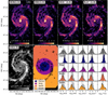 |
Fig. 1. Integrated intensity maps of dense gas tracers HCN, HNC, HCO+, and N2H+ from SWAN at a common resolution of 3″ (top row from left to right), as well as from 12CO (PAWS, bottom left). We divide the disk into a center and ring environment (Colombo et al. 2014a), and the outer disk into northern and southern halves (bottom row, second panel from left). We add contours of integrated N2H+ emission of 0.75, 2, and 4 K km/s to the environment map. We show the pixel-based integrated intensity distribution (in Kelvin kilometer per seconds) in various environments in the disk for all pixels in the FoV (colored shaded area), as well as for pixels where emission is detected (emission > 3σ, light gray shaded area) in the bottom right panels. The area of each histogram is normalized to unity. We indicate the median of all pixels (black dashed line) and median of masked pixels (dotted gray line) of each environment. The median represents the median value of logarithmic emission (med(log10(I))). Pixels with negative emission are excluded in the logarithmic scaling of the histograms. Since CO is detected across most of the FoV and is used as a prior in the creation of the moment-0 map (Sect. 2.2), its masked histogram distribution agrees well with the unmasked one. |
2.1. Dense gas and CO observations
The SWAN survey combines observations from the IRAM large program LP003 (PIs: E. Schinnerer, F. Bigiel) that used ∼214 hours of observations with NOEMA and 69 hours of observations with the 30m single dish to map 3 mm line emission from the central 5 × 7 kpc of the nearby galaxy M51. A more detailed description of this survey, the observations, data calibration, imaging and moment map creation can be found in a dedicated survey paper (Stuber et al. 2025). The NOEMA observations are performed by combining 17 pointings into a hexagonally spaced mosaic. The observations cover the ∼85 − 110 GHz range allowing for simultaneous observations of 9 molecular lines: 13CO(J = 1–0), HNCO(5–4), C18O(1–0), N2H+(1–0), HNC(1–0), HCO+(1–0), HCN(1–0), HNCO(4–3) as well as hyperfine transitions of C2H(1–0). Calibration and joint deconvolution of NOEMA and 30m data were carried out using the IRAM standard calibration pipeline in GILDAS (Gildas 2013). The native resolution of the data varies from ∼2.3″ (for 13CO) to 3.0″ (for HCN). The resulting dataset has an rms of ∼20 mK per 10 km s−1 channel for the brightest line (13CO(1–0)).
For this study, we utilize the N2H+, HCN, HNC and HCO+ data cubes at 10 km s−1 spectral resolution per channel and native spatial resolution, which we convolve to a common spatial resolution of 3″ (∼125 pc). For CO we directly use the PAWS data cube at 3″ spatial resolution1.
2.2. Moment map creation
The creation of moment-0 maps is described in Stuber et al. (2025). We integrate the molecular data cubes along their spectral axis using the PyStructure tool (den Brok et al. 2022; Neumann et al. 2023b). Creating moment maps is a common procedure to increase the signal-to-noise ratio (S/N), and to ease the comparison of the lines with each other and within the disk. These moment maps are created by using two selected priors, CO and HCN, to identify connected structures with emission above a selected S/N theshold of 2. This 3D signal mask is then used for integration. As described in Stuber et al. (2025) this ensures that all emission is captured in the final maps, including emission from the center, where CO is comparably faint, in contrast to HCN. The emission of HCN, HNC, HCO+, N2H+, and 12CO is then integrated over these structures, ensuring that the same pixels in the ppv cube are used for integration for all lines. This approach differs slightly from the one used in S23, where only 12CO was a prior for the mask instead of both CO and HCN. As described in Stuber et al. (2025), we interpolate and remove the area outside of the mosaic of pointings observed, as the noise increases toward the edges. The resulting maps have a resolution of 3″, and are regridded onto a hexagonal grid with four hexagonal spacings per beam (compare Fig. 1).
2.3. Ancillary data
We use ancillary data to generate maps of SFR surface density (ΣSFR), molecular gas mass surface density (Σmol), stellar mass surface density (Σ*) and dynamical equilibrium pressure (PDE) at a resolution of 3″. Those maps are incorporated into the PyStructure table and share the same hexagonal pixel grid as the molecular gas maps. All ancillary data are shown in Fig. 2.
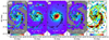 |
Fig. 2. Molecular gas mass surface densities, Σmol, star-formation rate surface densities, ΣSFR, stellar mass surface density, Σ*, dynamical equilibrium pressure, PDE, as well as CO velocity dispersion σCO at 3″ resolution. We show the contours of integrated N2H+ emission (0.75, 2,4 K km/s) on top. |
2.3.1. SFR tracers
We combine the Spitzer 24 μm map processed by Dumas et al. (2011), tracing recent star formation obscured by dust with 3″ resolution Hα maps from Kessler et al. (2020) tracing recent emission from HII regions powered by massive young stars. The 24 μm map is deconvolved with the so-called HiRes algorithm (Backus et al. 2005) to achieve a resolution of 2 − 3″ (Dumas et al. 2011). We obtain a map of SFR surface density (ΣSFR) via linear combination of the above mentioned SFR maps as described in Eq. 6 from Leroy et al. (2013) and correcting for inclination:
![Mathematical equation: $$ \begin{aligned} \Sigma _{\rm SFR}[M_\odot \, \mathrm{yr} ^{-1}\,&\mathrm{kpc} ^{-2}] = [ 634\, I_{\mathrm{H}\alpha } [\mathrm{erg} \,\mathrm{s} ^{-1}\, \mathrm{sr} ^{-1}\,\mathrm{cm} ^{-2}] \nonumber \\&+ 0.00325\,I_{24\upmu {m}} [\mathrm{MJy} \, \mathrm{sr} ^{-1}] ] \times \mathrm{cos} (i)\;. \end{aligned} $$](/articles/aa/full_html/2025/10/aa54473-25/aa54473-25-eq1.gif) (1)
(1)
2.3.2. Molecular gas mass surface density and CO(1–0) velocity dispersion
We utilize observations of 12CO(1–0) from the PAWS survey (Schinnerer et al. 2013). The 1″ resolution data are convolved to 3″ spatial and 10 km/s spectral resolution to match our observations. Applying a CO-to-H2 conversion factor αCO map to the integrated 12CO intensity (ICO) and correcting for inclination i yields the molecular gas mass surface density map via
 (2)
(2)
The spatially varying αCO is estimated based on modeling the observed 12CO(1–0), (2–1) and 13CO (1–0), (2–1) lines from SWAN and SMA imaging (den Brok et al. 2025). The measured values at 4″ resolution are extrapolated with a Gaussian process regression toward neighboring pixels to cover a larger area (compare area where Σmol is shown in Fig. 2). We test the impact of using different αCO prescriptions on our results in Appendix B, including Σmol calculated with a constant αCO and with a metallicity and stellar mass based αCO.
We further estimate the CO velocity dispersion following the prescription of Heyer et al. (2001), applied in, for example, Bešlic et al. (2021), Neumann et al. (2023a). This method estimates the ‘effective width’ of a line via the integrated intensity ICO (a.k.a. moment-0) and the peak intensity (Tpeak) at each pixel. Assuming a Gaussian line profile for these spectra with peak Tpeak, we can estimate the rms velocity dispersion of the line σmeasured via
 (3)
(3)
To account for line broadening caused by the instrument, we subtract the instrumental contribution σinstrument in quadrature (Rosolowsky & Leroy 2006; Sun et al. 2018). For M51, we use σinstrument estimates for CO from Sun et al. (2018) at 120 pc resolution (see their Eqs. 16 and 17 and Table 9).
2.3.3. Stellar mass map
We obtain stellar mass surface density maps (Σ*) based on Spitzer 3.6 μm maps from the Spitzer Survey of Stellar Structure in galaxies (S4G; Sheth et al. 2010) that are further corrected for dust emission (Querejeta et al. 2015). A more detailed description of this process and the obtained stellar mass map for M51 can be found in Querejeta et al. (2019). We convolve this map from 2.4″ resolution to our common resolution of 3″, and apply an inclination correction to obtain surface densities.
2.3.4. Dynamical equilibrium pressure
The dynamical equilibrium pressure (PDE) describes the ambient midplane pressure acting on the molecular gas disk, keeping it in vertical equilibrium and is set by the weight of the ISM in a galaxy’s gravitational potential (Elmegreen 1989; Ostriker et al. 2010; Field et al. 2011; Sun et al. 2020). We estimate the ISM pressure in each individual, cloud-scale region following the prescription from Sun et al. (2020, Eq. (16)). This “cloud-scale dynamical equilibrium pressure” formalism accounts for the weight of the gas from not only molecular cloud self-gravity but also external gravity by stars and gas across the galactic disk, as expressed below:
 (4)
(4)
Here, Σmol, θ is the molecular gas surface density at 3″ resolution (as derived in Sect. 2.3.2); Σmol, kpc is the corresponding kiloparsec-scale surface density, derived by convolving CO data from 3″ to 1 kpc resolution. Dcloud is the adapted cloud diameter, for which we use the beam size of 125 pc assuming a single cloud fills each beam. ρ*, kpc is the stellar mass volume density near the disk mid-plane, which we estimate from the kiloparsec-scale stellar mass surface density Σ*, kpc and stellar disk scale height H*:
 (5)
(5)
Based on Kregel et al. (2002) and Sun et al. (2020), we estimate H* from the stellar disk radial scale length R* = 7.3 × H*. For M51 we adopt R* = 4.0 ± 0.2 kpc from Dumas et al. (2011), adapted to our distance of D = 8.6 Mpc, while Dumas et al. (2011) used D = 8.2 Mpc.
3. Methodology and simulated data tests
We describe our methodology to obtain average intensities, average line ratios, as well as deriving relations between line intensities and line ratios and other galaxy parameters such as surface densities. To ensure that our results are not impacted by the different S/N of our dense gas tracing lines, we test all of the methods on a simple mock-dataset created based on the 12CO data, which we describe in more detail in Appendix A. In short, we scale the 12CO intensity in the CO data cube at 3″ resolution to lower values. We use four different scaling factors, chosen to be plausible estimates of our faintest observed line (N2H+(1–0)) from literature results. Those scaling factors further match our average HNC-to-12CO, HCO+-to-12CO and N2H+-to-12CO ratios (Table 2) plus an even smaller scaling factor to test the effect of even lower S/N.
Average line ratios of dense gas tracers.
For each scaled CO intensity we adjust the noise to simulate the corresponding S/N. The mock-data cubes are all then treated in the exact same way that we are treating our science data (Sect. 2.2), including the integration into the PyStructure to obtain moment maps that we can use for comparison (for more details see Appendix A.1).
To investigate potential environmental variations, we divide the disk of M51 into four regimes: A kinematically determined center and molecular gas-rich ring based on Colombo et al. (2014b) and sub-dividing the remaining disk into northern (north of the galaxy center) and southern (south of the galaxy center, see Fig. 1) halves. To highlight the importance of separating the environments, we note that the 12CO distribution reveals a brightness asymmetry in gas emission between the fainter northern and brighter southern spiral arm which is speculated to be caused M51b (e.g., Egusa et al. 2017). The center, which hosts both the nuclear bar, AGN, and low-inclined radio jet (Matsushita et al. 2015; Querejeta et al. 2016a), also provides physical conditions very different from the molecular ring and spiral arms further out. In addition to the full FoV, we will apply the methods mentioned in this section to the individual environments throughout this work.
3.1. Determination of average line ratios
Average global and regional line ratios between the emission of two lines are an effective way to measure the underlying physical conditions of the observed region, while reducing the impact of noise or peculiar outliers. We calculate average line ratios between different lines (Iline1, Iline2) by using the ratio of the integrated intensities in the full FoV. We integrate the intensity of all pixels in the moment-0 map within the FoV for the first line (line1) and divide by the integrated intensity of all pixels in the moment-0 map within the FoV for the second line (line2):
 (6)
(6)
Statistical uncertainties are then calculated following standard Gaussian error propagation. Our tests with the mock data (Appendix A.2) confirm that these methods robustly recover the expected line ratios. Masking will bias specifically datasets with lower S/N compared to those with higher S/N, and so do the other tested methods (median and mean line ratios; Appendix A.2).
3.2. Binning the data
Averaging data in increments of galactic parameters (e.g., surface density) is a useful technique (referred to as “binning” hereafter) to reduce the noise (i.e., negative and positive noise will cancel on average) and recover possible physical relations between intensity and those galactic parameters. To bin our data, we select bins of property A ranging from three times its average uncertainty (ΔA) up to the maximum value of A. For each bin, we first select the pixels that fall within the bin range and average the intensity of a line corresponding to those pixels, including nondetections (< 3σ). We calculate average line ratios R (both CO-line ratios and line ratios of dense gas lines) analogue to Eq. (6). As shown in Appendix A, excluding pixels will introduce biases (see also Neumann et al. 2023b).
In Fig. A.4 we show that with the method described above and by including all pixels we can recover the expected relation for this simple mock-data model. To ensure that the binned intensity measurements are not predominantly noise, we remove measurements where the binned average is below 5 times the corresponding statistical uncertainty. The statistical uncertainty is much lower than the average noise per bin (see Appendix A). We do not mask any data prior to the binning.
For binned intensities we provide the statistical uncertainty from error propagation. For binned line ratios R = M1/M2, the uncertainty is calculated as follows:
 (7)
(7)
With ΔMi being the relative error of binned intensity of line i = 1, 2, respectively. It is calculated following standard Gaussian error propagation  , for pixels a = 1…N and the error of the intensity at each pixel being sa. For ratios between fainter dense gas tracing lines, we further provide the 25th and 75th percentile range as visual guidance for each relation in addition to the statistical uncertainty presented above.
In our analysis, we want to find simple correlations between our observed line emission or line ratios and physical quantities to identify possible driving mechanisms. To quantify the slope and scatter of some of the observed trends, we fit a linear function of shape a × x + b (in log space) to the binned data with scipy-optimize, including the bin uncertainties. The scatter is then measured as the median absolute deviation of the residual intensity (or line ratio) within the fitted range after subtracting the best-fit relation. This scatter depends on the average S/N of a line and is used to compare how the scatter in each line’s intensity varies with different physical galactic parameters, rather than between different lines. As this scatter is measured with respect to a linear relation, it measures both a non-linear behavior indicative of secondary dependences, as well as the intrinsic uncertainty.
4. Comparison of line emission of dense gas tracers
HCN, HNC, and HCO+ are the favored tracers of dense gas in the extra-galactic community, as they are much brighter in emission than, for example, N2H+ and have higher critical densities than, for example, CO (e.g., see Table 4 of Schinnerer & Leroy 2024). Therefore, this theoretically allows them to trace regions of denser gas. They all correlate well with star-formation rate surface densities on galactic scales (Gao & Solomon 2004). To study the effect that the environment within M51 might have on these molecular lines, we compare their emission at cloud-scales (Sect. 4.2) and within larger scale galactic environments (northern and southern disk, ring, center, Fig. 1, Sect. 4.1). Comparing the emission of those dense gas tracing lines with emission of the Milky Way preferred dense gas tracer N2H+ will help understand their ability to trace dense regions. Lastly, we compare ratios of all dense gas tracers with 12CO, which are found to be density-sensitive at ≳100 pc scales (Leroy et al. 2017a; Jiménez-Donaire et al. 2019; Usero et al. 2015).
4.1. Distribution of HCN, HNC, HCO+, N2H+, and 12CO across environments
We show the emission of HCN, HNC, HCO+, N2H+ and 12CO in the central disk of M51 in Fig. 1. In our FoV, HCN, HNC, HCO+ and N2H+ are on average ∼29, 71, 38, 142 times fainter than 12CO emission (Table 2) and their emission is well correlated with each other (Spearman correlation coefficients all ρSp > 0.54), while their intensity probes about two orders of magnitude.
Figure 1 illustrates that all dense gas tracing lines are bright in the central few ∼100 pc, and along the molecular ring (Fig. 1, bottom right). A peculiar bright region, where N2H+ is brightest, is located at the southwestern brink of the molecular ring (compare also S23). 12CO is distributed in the FoV in a similar fashion to the dense gas tracers, yet its emission is less enhanced in the galaxy center compared to the disk than is seen for the dense gas tracing lines. Average line ratios among dense gas tracing lines and 12CO (Table 2) are enhanced in the central environment compared to other environments (factor of ∼1.6 − 2.3 from N2H+ to HCN between center and full FoV). Further, all line ratios among the dense gas tracers (HCN/HNC, HCN/HCO+, HNC/HCO+, HCN/N2H+, HNC/N2H+, HCO+/N2H+) vary significantly (> 3σ) between the central environment and other environments. All line ratios are increased in the center compared to other regions, except the HCO+/N2H+ line ratio, which is decreased.
While we see an asymmetry between a brighter southern and fainter northern arm in all lines, the overall intensity distribution of all molecules in the entire northern and southern disk match well (Fig. 1, bottom right panel). Still, average dense gas line ratios only agree between ring and northern disk environment, while line ratios in the southern disk are decreased (except the HCN/HNC ratio) by up to a factor of ∼1.9 compared to both ring and northern disk (Table 2). Line ratios with CO are increased in the southern disk compared to northern disk for N2H+ (factor ∼2) and HCO+ (factor ∼1/2).
4.2. Cloud-scale comparison of HCN, HNC, HCO+, N2H+, and 12CO
Larger-scale environments within galaxies are found to impact the physical conditions (Sun et al. 2022; Schinnerer & Leroy 2024) and thus emission pattern of molecules. Still, the exact mechanisms driving these large-scale changes, which we also see within M51 (Sect. 4.1) as well as variations within those environments are not well understood. In this section we analyze the cloud-scale variations within M51’s environments by comparing emission from the extragalactic dense gas tracers HCN, HNC and HCO+ with each other (Sect. 4.2.1) and with the much fainter dense gas tracer N2H+ (Sect. 4.2.2). Cloud-scale variations of density sensitive line ratios with 12CO are analyzed in Sect. 4.2.3.
4.2.1. Correlation between HCN, HCO+, and HNC
In Fig. 3 we display the cloud-scale distribution of line ratios HCN/HNC, HCN/HCO+, and HNC/HCO+ where for visual purpose only line ratios for detected sightlines (> 3σ) are shown in the maps. Of all line combinations, the HCN/HNC line ratio has the smallest variations within the disk (±0.2 dex to the global average). It is slightly increased in the northern disk and molecular ring compared to the southern half and spiral arms.
The line ratios with HCO+ exhibit larger variations (±0.2 − 0.4 dex to the global average). HCN/HCO+ increases azimuthally symmetrically in the center out to a radius of ∼1 kpc. The line ratio in the southern arm is smaller than the global average, but shows little variations, while there are ∼ beam-sized variations in the line ratios in the northern arm. Similarly to the HCN/HCO+ ratio, the HNC/HCO+ ratio is increased in the center relative to the global average and spiral arms, with a slightly stronger azimuthally asymmetric increase toward the southwestern half of center and molecular ring up to a radius of ∼1.5 kpc, in accordance with the asymmetric HCN/HNC distribution. Beam-sized variations in the HNC/HCO+ ratio are seen across the entire disk.
In summary, both HCN and HNC are enhanced in the central ∼1 − 1.5 kpc compared to HCO+ and compared to the spiral arms and global average.
4.2.2. Comparing line intensities to N2H+
Unlike HCN, HNC and HCO+, emission from the molecular ion N2H+ has been the favored tracer of dense regions in Milky Way clouds (e.g., Kauffmann et al. 2017; Pety et al. 2017). We show the spatial distribution of line ratios of HCN, HNC and HCO+ with N2H+ emission in Fig. 4. The intensity scale depicts the same range (in dex) around the average line ratio as in Fig. 3. The variations seen in the N2H+-line ratios are larger (≳0.5 dex around the global average) than the variations seen among the brighter dense gas lines (e.g., HCN/HNC).
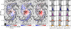 |
Fig. 3. Left panel: Line ratios of integrated line emission from dense gas tracers HCN, HNC, and HCO+. For visual purposes, we only show line ratios for significant detected pixels (> 3σ), but include nondetections in all calculations. We mark pixels in which CO is detected (gray points) and the center of the galaxy (green plus). The intensity scale is centered logarithmically on the average line ratios (log10R, with R from Table 2) determined for all pixels in the FoV, including nondetections. The average line ratio (log10R) and the total range of 1 dex covered by the color bar are indicated by the dashed black line and gray shaded area in the right panel. We show contours of integrated N2H+ emission (0.75, 3 K km/s) on top. Right panel: Histogram of line ratios per environment analogous to Fig. 1 but for HCN/HNC, HCN/HCO+, and HNC/HCO+ (colored histograms). We indicate the number of pixels shown in the histogram (top right corner), which varies slightly, as values with negative noise cannot be shown in the logarithmic scale. |
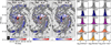 |
Fig. 4. Same as Fig. 3 but for the HCN-to-N2H+, HNC-to-N2H+, and HCO+-to-N2H+ line ratios. The colorbar spans the same 1 dex range as in Fig. 3, and is centered logarithmically on the average line ratios (log10R, with R from Table 2). |
All N2H+ line ratios increase compared to the global average in a region northeast of the center of a few ∼100 pc in size, and decrease at even larger radii east of the center. The increase in line ratios is strongest for HCN/N2H+ (∼0.5dex) and weakest for HCO+/N2H+ (∼0.1dex) compared to the global average. N2H+ is not detected in the southwestern half of the center and molecular ring, where the HNC/HCO+ line ratios are increased.
N2H+ line ratios are decreased in the spiral arms in pixels where N2H+ is significantly detected compared to the global average. Again, the strongest variations in line ratios are seen for HCN/N2H+ (±0.5 dex across many pixels), the smallest for HCO+/N2H+ (mostly ±0.2 dex with only few pixels with larger line ratios).
4.2.3. Proposed average gas density tracer: Line ratios with CO
While dense gas tracers such as HCN, HNC, and HCO+ are efficiently emitting at densities above their critical densities, less efficient emission from sub-critical density regions can still significantly contribute to the total integrated intensity of those lines (Kauffmann et al. 2017; Leroy et al. 2017b). In spite of those effects, line ratios with the bulk molecular tracer CO are found to be sensitive to the average gas density (e.g., review by Neumann et al. 2023a; Schinnerer & Leroy 2024; Neumann et al. 2025). We show the spatial distribution of 12CO line ratios of HCN, HNC, HCO+, and N2H+ in Fig. 5. We refer to these line ratios as  .
.
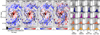 |
Fig. 5. Same as Figs. 3 and 4 but for line ratios with CO. In contrast to the previous figures, the colorbar spans a larger range of 1.5 dex, centered on the average line ratios (Table 2), and we add line ratios in pixels with nondetections. Since we show the logarithmic line ratio, negative values that arise from negative noise cannot be shown in either the spatial map or the histograms. We mark pixels where CO is significantly detected, but the line ratio cannot be shown in logarithmic scaling in dark gray. The contours depict integrated N2H+ emission at 0.75 and 3 K km/s. |
We find that for all lines,  increases in the center and molecular ring compared to the global average, with a particular increase of up to ≳0.8 dex in an elongated feature that expands toward northeast of the center, which corresponds to the same region where N2H+ line ratios are increased. Visually, the HCO+/CO ratio is less enhanced in the central ∼2 kpc than the HCN/CO and HNC/CO ratio. All
  are decreased in the spiral arms compared to the global average, and exhibit a gradient from low to high line ratios across the arms from trailing to leading side, which is more prominent in the southern arm.
4.3. Average line intensities and CO line ratios compared to N2H+ emission
Combining the results from Sects. 4.2.2 and 4.2.3, we see clear variations in line ratios both per galactic environment and from cloud-to-cloud. To quantify the impact of these variations on the average N2H+ emission, we probe the binned intensity of HCN, HNC, HCO+ as well as their binned 12CO line ratios as a function of N2H+ emission in Fig. 6 for the total FoV and the individual environments. Fit parameters obtained by fitting the binned intensities and binned CO line ratios as function of N2H+ emission and N2H+/CO (Sect. 3.2) are provided in Table 3.
Fitting average line intensities and average CO-line ratios as a function of N2H+ intensity or N2H+/CO ratio per environment.
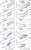 |
Fig. 6. Average intensities of HCN, HNC, and HCO+ as function of N2H+ intensity (left) as well as average 12CO line ratios of HCN, HNC, and HCO+ (right) as function of the N2H+/CO line ratio emission. We do not apply any masking, but utilize all pixels in the FoV. We show the binned intensities and binned line ratios for the total FoV (top) as well as for individual environments (Fig. 1). We provide lines of constant slopes in log space for visual guidance (dashed black lines). The bins cover a range between three times the average N2H+ (N2H+/CO) uncertainty up to the maximum N2H+ intensity (N2H+/CO line ratio). |
Across the total FoV, the average HCN, HNC and HCO+ emission agrees well with the N2H+ emission (slopes are within 3σ of unity), while the average 12CO emission is significantly sub-linearly related with N2H+ emission across the full FoV (Table 3) and our defined environments. This is in agreement with the super-linear inverse N2H+-to-12CO and N2H+-to-HCN relations, found by S23 using the preliminary SWAN data. The scatter in the full FoV for the line versus N2H+ relation is highest for HCN, followed by HNC, HCO+ and 12CO as function of N2H+ intensity (Table 3). In contrast to 12CO, the slopes of HCN, HNC and HCO+ as function of N2H+ intensity agree well with each other across all environments. Still, their slopes are sub-linear in the center and ring, and super-linear in northern and southern disk.
While it is unclear whether  is sensitive to the average cloud density similar to what is proposed for
  , we test the
  versus
  relation (Fig. 6) and list scatter and slopes in Table 3. As the N2H+ molecule is chemically bound in existence to very dense and cold regions where CO, its main reactant, is frozen to dust grains, its emission is found to depend non-linearly on column density in clouds in the Milky Way (Tafalla et al. 2023). On our ∼100 pc scales we find
  to depend mostly sub-linearly on
  across the environments. The slopes range between very low values 0.05 − 0.44 in ring, northern and southern disk, up to slopes of ∼1.0 in the center. The scatter of the
  versus
  relation is the largest among all relations tested.
The 12CO line ratios of HCN, HNC, and HCO+ as a function of N2H+ intensity reveal significantly sub-linear slopes across all environments, with slopes as low as 0.14 for  versus N2H+ in the ring and as large as 0.68 for
  in the northern disk. Despite the low slopes, the average scatter of
  versus N2H+ are the lowest among all relations tested, and is particularly low for the
  versus N2H+ relation.
5. Environmental impact: Physical parameters that drive line emission
While all dense gas tracers are similarly distributed in the disk of M51, systematic variations as function of both larger-scale and cloud-scale environment are seen (see Sect. 4). Here we aim to identify the physical conditions that best describe the intensity distribution of dense gas tracing molecules and variations between them by comparing the dense gas emission with different physical parameters, including Σmol, Σ*, ΣSFR, PDE, σCO and galactocentric radius. All values are corrected for inclination and described in more detail in Sect. 2. Figure 2 shows our estimates of Σmol, ΣSFR, Σ*, PDE and σCO across our FoV.
We test both the intensity of HCN, HNC, HCO+, and N2H+ and their ratios with the 12CO line as a function of this set of properties in Sects. 5.1 and 5.2, respectively. In Sect. 5.3 we investigate how line ratios between dense gas lines depend on the environmental properties.
5.1. Line intensity as a function of physical parameters
We show the binned average intensities of HCN, HNC, HCO+, N2H+, and 12CO as a function of physical parameters in Fig. 7. The same analysis per spatially distinct environment (center, ring, north, south), as well as a pixel-by-pixel version of these plots is provided in Appendices D and E, respectively. We provide fit parameters from the full FoV in Fig. 7 and Table D.1, and for each environment in Appendix D. The scatter with respect to the full FoV fits is depicted in Fig. 8. Further, we show Spearman correlation coefficients of the full FoV in Fig. 9.
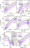 |
Fig. 7. Average line intensity, ILine, as a function of surface densities of molecular gas mass (Σmol), stellar mass (Σ*), and star-formation rate (ΣSFR), as well as velocity dispersion (σCO), dynamical equilibrium pressure (PDE), and galactocentric radius for all dense gas tracers. Shaded areas mark the standard deviation per bin. The 12CO intensity scaled by a factor of 1/10 is added for comparison (gray line). For r > 2.2 kpc, the shape of our FoV leads to incomplete sampling of these radial bins (gray shaded area). The obtained slopes for a linear fit (in log space) to the binned averages are provided in each panel. |
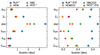 |
Fig. 8. Average scatter of dense gas line intensity (left panel) and average dense gas to CO line ratios (right panel) as a function of physical galactic properties with respect to a linear relation (methodology described in Sect. 3.2). The impact of S/N on this plot is shown in Appendix A.4. |
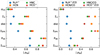 |
Fig. 9. Spearman correlation coefficients of line intensity (left panel) and average dense gas to CO line ratios (right panel) as a function of physical galactic properties (Sect. 2.3). An increased S/N will directly result in a lower correlation coefficient. We therefore expect higher correlation coefficients for HCN, followed by HCO+, then HNC, then N2H+ as a function of the same galactic properties. All p values are below 5% except p values for the line/CO ratios as a function of σCO. |
The average line intensity of all lines is monotonically positively correlated with Σmol and PDE (deviations from a monotonic relation ≲0.2 dex) and non-monotonically with Σ*, ΣSFR, σCO, and galactocentric distance, which suggests secondary dependences. Consequently, the scatter with respect to a linear relation between line intensity and physical properties is lowest (Fig. 8) and Spearman correlation coefficients are highest for PDE and Σmol (Fig. 9).
Fitted slopes of average intensity as function of Σmol range from unity (CO, HCN), to significantly super-linear (HNC, HCO+, N2H+). These values confirm that N2H+ has a significantly steeper dependence on Σmol than the other lines, while HCN has a similar shallower dependence on Σmol than CO does. While slightly reduced in the center, the slopes obtained in the environments are consistent with this result (Appendix D). We note a turn-up in the N2H+-to-Σmol relation at high values of Σmol, where the trend steepens, which corresponds to the N2H+-brightest region located at the southwestern brink of the molecular ring (Sect. 4.1).
Slopes of average intensity as function of PDE range from significantly sub-linear (CO, HCN, HNC, HCO+) to linear (N2H+) and while they vary slightly with environment (Appendix D), the increased order or slopes from CO to N2H+ is mostly consistent with the full FoV environment. The dependence of CO and HCN on PDE is significantly different.
As the relations of line intensity with other physical galactic parameters are depicting larger variations deviating from a straight-line relation, we suspect a dependence on secondary properties. We find the following: Average line intensities all increase with increasing Σ*, except for a plateau (N2H+, HNC, HCN) or decline (CO, HCO+) at Σ* ∼2 − 7 × 10⁹ M⊙ kpc−2, which corresponds to radii of r ∼ 0.2 − 1 kpc. This is consistent with the flatter trend seen in line ratio as function of galactocentric radius.
All lines are similarly well correlated with ΣSFR up to values of 4 × 10⁻¹ M⊙ yr−1 kpc−2, where the distribution flattens. We identify a shallower distribution in the northern disk compared to the other environments, which, when averaged, produces the flattening (Appendix D). The same effect is driving the flattening seen with σCO.
5.2. Line ratios with CO as a function of physical parameters
Ratios between dense gas tracers and bulk tracer CO are found to be density sensitive (e.g., Leroy et al. 2017a; Schinnerer & Leroy 2024). To explore the physical mechanisms driving these CO line ratios, we show  ,
,  ,
,  and
and  as function of physical properties Σmol, Σ*, ΣSFR, σCO, PDE and galactocentric radius in Fig. 10. We provide fit slopes when fitting a linear to the binned data in Fig. 10 and for the distinct environments and full FoV in Appendix D.
The average  follows a nearly straight-line relation with Σmol and PDE, albeit the
  -to-Σmol relation steepens at high values of Σmol. Ratios related with other parameters depict stronger variations and deviations from a linear relation. Despite this linear dependence of CO line ratios and Σmol, fitted slopes are surprisingly low, with slopes for
  consistent with being zero. Spearman correlation coefficients are lowest for
  -to-Σmol (ρSp ≲ 0.35) compared to any other property (except σCO, Fig. 9). This indicates that in the full FoV,
  is nearly independent of Σmol at cloud-scales in M51.
We explore possible biases that affect these measurements, such as different estimates of Σmol (Appendix B), the impact of the AGN (Appendix C), or the relation within individual environments (Appendix D). All tests agree that the  ratio has a very shallow and variable dependence on Σmol, that even turns negative depending on the prescription used to estimate Σmol and the environment studied.
  and
and  behave similarly, although they generally have steeper slopes as a function of Σmol. Within distinct environments, the slope of the
  to Σmol relation varies from −0.04 ± 0.1 in the center up to 0.8 ± 0.05 in the molecular ring (Appendix D). Removing the central 1 kpc data including the brightest pixels of HCN, HNC and HCO+, increases the slopes of all
  to Σmol relations, particularly for the
  ratio (i.e., slope of 0.36 ± 0.02 for
  , and 0.68 ± 0.06 for
  ; Appendix C). Even in the environments outside of the center, the
  to Σmol relation is shallower than common literature results (compare Sect. 6).
The dependence of  to PDE is positive albeit shallow across all environments (Appendix D) with lowest slopes for
  followed by
  ,
,  and
and  . Spearman correlation coefficients are higher than compared to Σmol, but lower than Σ*, r and ΣSFR (Fig. 9. While the scatter relative to a linear correlation (Fig. 8) is lower for
  ,
,  and
and  as function of PDE compared to Σmol, the scatter is even lower for other physical parameters, i.e. ΣSFR for
  and Σ* for
  . Similarly, Spearman correlation coefficients (Fig. 9) are highest for
  for all lines except N2H+ as function of Σ*, r and ΣSFR, followed by PDE, Σmol and are lowest for σCO. Due to the low S/N of the N2H+ emission, the variation seen in the scatter and Spearman coefficients of
  as function of physical parameters is consistent with noise (compare Appendix A.4). Similar to Sect. 5.1, the 12CO line ratios as function of Σ* and radius change slope at radii of ∼0.2 − 1.2 kpc.
5.3. Dense gas line ratios as a function of physical parameters
We show average line ratios between HCN, HNC and HCO+ and line ratios between those lines and N2H+ as function of Σmol, Σ*, ΣSFR, σCO, galactocentric radius and PDE in Fig. 11, and separated into environments in Appendix D. Among the brighter dense gas tracers HCN, HNC and HCO+ we find the largest dependence on physical properties of line ratios with HCO+, with a nearly linear dependence with Σmol and radius. Consistent with findings in Sect. 4.2.1, the HCN/HNC ratio is basically independent of physical properties or dependences are very shallow (slopes range from −0.14 to 0.11, Table 4). HCN/HCO+ is positively correlated with ΣSFR and negatively correlated with radius and Σmol.
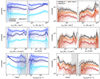 |
Fig. 11. Average line ratios of HCN/HNC, HCN/HCO+ and HNC/HCO+ (left panels) as function of physical properties as well as for HCN/N2H+, HNC/N2H+, HCO+/N2H+ (right panels). Error bars depict the 25/75th percentiles. |
Fitted slopes to binned line ratios as function of Σmol, ΣSFR, Σ*, PDE, σCO and radius.
Ratios of HCN, HNC and HCO+ with N2H+ show no clear linear dependences on any of the properties. All ratios monotonically decrease at high values of Σmol and PDE and all except for the HCO+/N2H+ ratio decrease with galactocentric radius. We find the steepest slopes for the HCN/N2H+-to-Σmol relation (−0.42) and shallowest for HCO+/N2H+-to-Σmol (−0.2). A local minima in N2H+ line ratios as function of both Σ* and radius can be associated with radii of r ∼ 0.2 − 1 kpc.
We highlight the impact environment has on the slopes of average N2H+ line ratios as function of Σmol in Fig. 12. We show the same relation for all physical properties in Appendix D, but provide here a version easier to compare. In contrast to the other environments, the slope measured in the ring environment is significantly negative with a steep slope of −0.63 (see the figure caption).
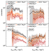 |
Fig. 12. Same as right panels of Fig. 11, but only for relations with Σmol and separated into the different environments. We note that fitting the binned averages as function of Σmol results in slopes that are within 5σ to a slope of zero for all line ratios as function of Σmol, except for the ring environment, where the slopes are significantly negative. The slopes for the HCN-, HNC- and HCO+-to-N2H+ line ratio as function of Σmol in the ring environment are −0.63 ± 0.04, −0.48 ± 0.04 and −0.46 ± 0.04, respectively. |
Our results suggest that the line most closely related to N2H+ is HCO+, as the HCO+/N2H+ line ratio shows the smallest slopes as function of galactic parameters compared to the HCN/N2H+ and HNC/N2H+ ratios. The most different to N2H+ is the molecule HCN, with the largest line-ratio to galactic property slope of HCN/N2H+-to-Σmol of –0.42. The molecular line emission closest to the HCN(1–0) emission is HNC(1–0), as the HCN/HNC line ratio is smaller than HCN line ratios with HCO+ or N2H+. The largest differences between N2H+ ratios (if present) is revealed by Σmol, followed by galactocentric radius, Σ* and PDE. The largest difference between line ratios among HCN, HNC and HCO+ is revealed by Σ*, followed by galactocentric radius and Σmol. In summary, at our 125 pc scales, there are no two molecules that have the exact same emission pattern across all environmental conditions.
6. Discussion on dense gas in M51
Our observations of HCN, HNC, HCO+ and N2H+ in the disk of M51 cover different galactic environments, including spiral arms, a molecular ring and AGN affected center, and span a range of physical conditions. We discuss the impact of environment and physical conditions on the dense gas emission, and ultimately the ability of this emission to trace dense regions.
6.1. Dense gas tracers as reliable tracers of dense gas
The emission of N2H+, which originates from regions where 12CO is frozen out on dust grains, is undisputedly an ideal indicator of cold and dense regions within Milky Way clouds, and likely also a good indicator of dense regions in M51. The emission of a “dense gas tracer” is thus expected to agree reasonably well with the emission of N2H+. Our data show that, in contrast to the emission of the bulk tracer 12CO, the emission of HCN, HNC and HCO+ performs well at tracing N2H+ emission linearly in our FoV, but this correlation clearly varies with environment. When compared on cloud-scales and across the environments and physical conditions present in M51, the emission of HCO+ is favored over the emission of HCN and HNC, as it is more closely related to the N2H+ emission and has higher values of ρSp across the environments when compared to Σmol despite being fainter than HCN on average.
When comparing the emission of dense gas molecules with estimates of Σmol, often assumed to be indicative of the gas volume density, we find that the relation between HCN and Σmol is more similar (in slope) to the relation between CO and Σmol, while the relationship between HCO+ and Σmol (in slope) is closer to the relationship between N2H+ and Σmol. At much smaller than our resolutions within three individual clouds in the Milky Way, Tafalla et al. (2023) find strong and similar correlations between HCN, HNC, and HCO+ emission and column density and clear deviations from the CO relation. Tafalla et al. (2023) further find that N2H+ emission rises more steeply with estimates of column density than any of the other lines, and emission only arises above column densities of 1022 cm−2 (corresponding to Σmol∼2 × 10⁸ M⊙/kpc2). This is in disagreement with our general similar trends found between N2H+, HCO+, HCN and HNC, but at our resolution (and different measurements of Σmol). However, we note that in our observations, N2H+ emission as function of Σmol changes slope at highest values of Σmol (≳2 × 10⁸ M⊙ kpc−2), which is not the case for the other lines. While this could point to a boosted production of N2H+ above a threshold of Σmol, in agreement with Barnes et al. (2020), Tafalla et al. (2023), we note that at our resolution, we are likely averaging several clouds within one beam and do not expect to recover the same relation. Further, this steepening in the N2H+-to-Σmol relation is mainly driven by the N2H+-brightest region located at the southwestern brink of the molecular ring. We discuss possible mechanisms responsible for the high N2H+ emission in Sect. 6.3.
The 12CO line ratios depend super- or sub-linearly on the N2H+/CO ratio depending on the environment, suggesting that the molecules are not similarly sensitive to density. The scatter is minimized when comparing CO line ratios directly with N2H+ intensity, albeit the relations are significantly sub-linear with exception of the central environment. When comparing their emission with estimates of surface density, Σmol, a commonly used proxy of gas density, we find that the HCN/12CO line ratio is not significantly correlated with Σmol across the FoV of our SWAN data, with Spearman correlation coefficients of ρSp ∼ 0.3, which are smaller than when comparing HCN/12CO to any other physical parameter (except σCO). Typical HCN/CO line ratios from lower-resolution surveys follow a relation with Σmol of slope ∼0.65 (Neumann et al. 2025), which is obtained by combining ≳ kiloparsec-scale observations of 31 local spiral galaxies in the EMPIRE survey (Jiménez-Donaire et al. 2019) and ALMOND survey (Neumann et al. 2023a). Similarly, the 300 pc resolution observations in NGC 4321 match these literature slopes well (Neumann et al. 2024, Fig. 13) Even estimates from three Milky Way clouds find slopes in the HCN/CO-to-Σmol relation of ∼0.71 (Tafalla et al. 2023). The relation found in our data, both from the total FoV as well as obtained from individual environments, is significantly shallower and weaker (ρSp ≲ 0.4) than any of these literature correlations or even negative, as we show in Fig. 13.
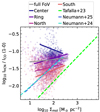 |
Fig. 13. Literature comparison of fits best describing HCN/CO as a function of Σmol. We include estimates from Milky Way clouds (Tafalla et al. 2023, dashed green line), fits of individual environments and full FoV in M51 (this work, solid lines), fits based on HCN/CO at 260 pc resolution in NGC 4321 (Neumann et al. 2024), and fits based on 31 local spiral galaxies from the ALMOND (Neumann et al. 2023a) and EMPIRE (Jiménez-Donaire et al. 2019) surveys at ∼kiloparsec resolution (Neumann et al. 2025). We add our HCN/CO observations for visual comparison for each environment within M51 (open colored circles). |
Our results are similar to 150 pc resolution observations in the central 1 kpc of NGC 6946 (Eibensteiner et al. 2022), that only find a weak and shallow correlation between HCN(1–0)/CO(2–1) and CO(2–1) intensity as proxy for Σmol (slopes of ∼0.23, ρSp ∼ 0.39), and instead find a stronger correlation for HNC/CO followed by HCO+/CO. In their observations, HCO+ is best correlated with ΣSFR. NGC 6946 does not exhibit signs to host an AGN that could explain an enhancement in HCN emission.
Our results show that in the inner disk of M51 at cloud scales, the HCN/CO ratio does not trace Σmol well at all and also the HCO+/CO or HNC/CO ratios are shallow. Removing central apertures (Appendix C) or using different prescriptions to calculate Σmol (Appendix B) do not resolve this issue. While we find steeper slopes for some of those treatments, the high variability of the slope with aperture and Σmol prescription makes the HCN/CO ratio a very questionable tracer of Σmol in M51. Spearman correlation coefficients do not change when removing central apertures, and are all significantly lower than when comparing RCOLine to any other physical parameter except σCO. The dynamic range of Σmol is not reduced when removing the central 1 kpc (Appendix C). While the N2H+/CO-to-Σmol relation reveals higher slopes, those slopes vary greatly across the different environments.
Potentially, the Line/CO ratio is not solely dependent on gas density, but other conditions that are possibly more extreme in the interacting M51 than in the other galaxies mentioned above. However, since this is the first time that observations at this resolution across such a large FoV have been taken, it is unclear whether the conditions in M51 are peculiar, or whether the resolution is causing the differences.
6.2. Physical conditions driving gas emission
While molecular gas mass surface density is commonly used as a proxy for the volume density and thought to directly drive the emission of dense gas molecules, dynamical equilibrium pressure is suggested to directly determine the ability of gas to form stars (e.g., Usero et al. 2015; Jiménez-Donaire et al. 2019; Neumann et al. 2025). In comparison to Σmol, we find less variation in the slopes of R as a function of PDE across environments (i.e., no negative slopes), but slopes are similarly shallow. In contrast to a linear correlation, Neumann et al. (2024) suggests a dynamical equilibrium pressure threshold above which the HCN/CO to PDE and HCN/SFR to PDE relations change slope, falling at PDE∼4 × 105kB K cm−3 for HCN/CO versus PDE and PDE ∼ 1 × 106kB K cm−3 for HCN/SFR versus PDE. Considering that this threshold of the measured PDE may change with resolution (Sun et al. 2020), this is in agreement with various theoretical works that suggest that clouds decouple from their environment above a pressure threshold and collapse in a universal fashion (e.g., Ostriker et al. 2010; Ostriker & Kim 2022). Our data reveals no clear change in the HCN/CO versus PDE relation, despite covering the same dynamic range, but all line ratios with N2H+ visually appear to turn from positive to negative slopes at PDE∼1 × 10⁶kBK cm−3. At high pressures the fractions of immediately star forming gas is expected to increase so that the ratio of higher critical density N2H+ to HCN or HCO+ is expected to change. As shown by sub-cloud-scale simulations by Priestley et al. (2023), N2H+ largely traces gas in such dense regions that irreversibly collapse, in contrast to HCN, HNC, and HCO+ which also trace a significant amount of gas that will not eventually form stars, in agreement with our observations.
While PDE and Σmol are promising drivers of the gas emission, line ratios with CO have an increased scatter when compared to those physical properties compared to others. Despite there being secondary trends and local minima in relations with other physical quantities, the scatter measured with respect to a linear relation of the HCO+/CO ratio is minimized when compared to Σ*, whereas the scatter of HCN/CO is smallest when compared to Σ* and ΣSFR. Both Σ* and ΣSFR however depict local minima and changes of slopes that might be connected with PDE as follows. Figure 14 shows the ratio of internal to dynamical equilibrium pressure (Pint/PDE). The internal pressure Pint refers to the pressure inside a molecular cloud, likely dominated by turbulence (hence often known as Pturb, which supports the cloud against its own weight and the weight of the ambient gas (e.g., Sun et al. 2020, and references within). A ratio of Pint/PDE of unity might suggest that the cloud is pressure-confined and in approximate balance with its environments. A ratio larger than unity suggests that molecular gas is overpressurized compared to its surrounding environment. This ratio is below unity in the central ∼3 kpc, except for the very central few ∼100 pc, suggesting that the clouds are not in equilibrium with their surrounding environment. The Pint/PDE ratio further reveals an asymmetry between the northern and southern spiral arms, which we discuss in more detail below. The decrease of Pint/PDE in the center coincides spatially with the shallower relation between line intensity, CO line ratios and Σ* or radius found at radii of ∼0.2 − 1.2 kpc. In comparison, the bulge of M51 is thought to be only ∼450 × 650 pc in size (Lamers et al. 2002). In the central environment coinciding with this region, emission of HCN, HNC and HCO+ is sublinearly correlated with Σmol, and CO line ratios are negatively correlated with Σmol while being most steeply correlated with both Σ* and σCO compared to other environments.
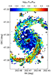 |
Fig. 14. Logarithmic ratio of Pint/PDE. We calculate Pint = 3/2 Σmol × σCO2/D according to Eq. 10 from Sun et al. (2020) and with D = 125 pc. We show N2H+ contours at 0.5, 2, and 4 K. |
Furthermore, the HCN/HCO+ (and HNC/HCO+) ratio is higher in the central ∼1.5 kpc. A possible mechanism to regulate the molecular line emission in the center could be provided by a high cosmic ray ionization rate (CRIR). A high CRIR can increase the formation of HCO+ (e.g., Harada et al. 2019), by increasing the abundance of H3+, which is a key molecule for HCO+ formation. This occurs via the ionization of H2 to H2+, which can form H3+ in a secondary step (e.g., Le Petit et al. 2016). However, in lower-density environments or at high cosmic ray ionization rates, the electrons produced via the ionization of H2 recombine with and destroy H3+ and HCO+ (Le Petit et al. 2016), yielding an equilibrium HCO+ abundance that is independent of the cosmic ray ionization rate. An increased free electron fraction also enhances the HCN excitation rate (Krolik & Kallman 1983; Maloney et al. 1996; Papadopoulos 2007; Goldsmith & Kauffmann 2017). Combined, this might lead to an increased HCN to HCO+ emission ratio.
While some studies find a correlation between cosmic ray ionization rates and X-ray emission produced by inverse Compton scattering of hot gas (Schober et al. 2015), the contribution of this mechanism to the total X-ray flux is expected to be fairly small for local non-starbursting galaxies. Zhang et al. (2025) find a sharp decrease in the surface brightness profile of hot gas from X-ray observations with Chandra in M51 at r ∼ 2 kpc as well as a steeper relation between kiloparsec-scale HCN emission in the central ∼2 kpc and hot gas luminosity compared to the disk. They further conclude a negligible impact of the AGN on the hot X-ray gas luminosities, and suggest that instead core-collapse supernovae (SN) dominate the energy source in M51’s center.
Increased ionization rates can also be found in the CMZ of the Milky Way compared to its disk, where they also result in increased gas temperatures (Oka et al. 2019; Indriolo et al. 2015). Variations in kinetic gas temperature can increase the scatter of HCN intensity as function of gas column density (Tafalla et al. 2023). With the gas temperature in merging galaxy systems generally being increased (Schinnerer & Leroy 2024), this can increase the scatter of the HCN/CO ratio. However, kinetic gas temperature estimates by den Brok et al. (2025) combining SWAN and SMA CO and CO isotopologue observations reveal average gas temperatures in our FoV of ∼13 ± 5 K with no significant increase toward M51’s center. High HCN/HCO+ ratios similar to our results (Fig. 3) are also common in centers in Ultra Luminous Infrared Galaxies (ULIRGs, e.g., Aalto 2005; Imanishi et al. 2023), LIRGs (Papadopoulos 2007) as well as centers hosting AGNs of normal galaxies (Usero et al. 2004; Nakajima et al. 2023), including M 51 (Kohno 2005). However, the molecular gas in centers of ULIRGs is often warm (i.e., T ≳ 100 K Imanishi et al. 2023), which is – again – not the case for M51’s center.
The HCN/HNC ratio has been suggested to track kinetic gas temperature in Milky Way clouds (Hacar et al. 2020). We show the HCN/HNC ratio as function of Tkin from den Brok et al. (2025) in Fig. 15. Theoretically, at a temperature of T > 30 K, the equal formation of HCN and HNC is offset by the conversion of HNC into HCN. We find no clear correlation between our line ratios and kinetic gas temperature, in agreement with other extragalactic studies at kiloparsec scales in the EMPIRE galaxies (Eibensteiner et al. 2022) and ∼100 pc in NGC 6946, M51, NGC 3627 (Eibensteiner et al. 2022) and M83 (Harada et al. 2024). The latter find HCN/HNC to depend on UV illumination instead.
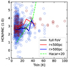 |
Fig. 15. HCN/HNC line ratio from this work as a function of kinetic gas temperature measurements at 4″ resolution from den Brok et al. (2025). We separate pixels in the center (r < 500 pc, red points) and disk (r > 500 pc, blue points), and provide binned estimates for the full FoV (black line), center, and disk (red, blue, respectively) in steps of 5K in the range ∼10 − 50 K, suggested by Hacar et al. (2020). We add the fitted relation from Hacar et al. (2020) (dashed green line). |
We note that the effects of AGN feedback on the molecular ISM and the extent of this impact is not well known in M 51. Our data reveal both a clear enhancement in line intensities and line ratios in the very center (r ≲ 500 pc, i.e., Fig. 5), which might agree with radio emission from a low-inclined radio jet (Matsushita et al. 2015; Querejeta et al. 2016a). Querejeta et al. (2019) find a clear enhancement of HCN/CO due to the AGN in M51’s center at 4″ resolution. In fact, observations of dense-gas tracing molecules such as HCN, HCO+ and HNC in galactic starburst-driven (NGC 253; Meier et al. 2015) or AGN-driven outflows (Mrk231; NGC 1068; NGC 1377; Aalto et al. 2012, 2015; García-Burillo et al. 2014; Aalto et al. 2020) at resolutions down to a few pc suggest the survival, formation and/or emission enhancement of dense gas in outflows (Jørgensen et al. 2004; Tafalla et al. 2010; Aalto et al. 2015). The nuclear outflow will be discussed in much greater detail in upcoming papers (Thorp et al. in prep.; Usero et al. in prep.).
6.3. Anomalies in the molecular ring
The molecular ring in M51 stands out as a peculiar environment: Average line intensities of HCN, HCO+ and HNC follow N2H+ emission only sub-linearly (Table 3), and consequently, line ratios with N2H+ as function of Σmol exhibit significantly negative trends (Fig. 11). The N2H+/CO-to-Σmol relation in the ring has the largest slope (0.8 ± 0.05; Appendix D) compared to all other environments and all other CO line ratios. The ring environment has the largest absolute number of pixels in which N2H+ is detected (> 3σ) compared to the other environments. As it has the second highest fraction of detected pixels (28%, compared to the center with 52%), effects of S/N and beam dilution are expected to play a much lesser role than for the northern and southern spiral arm. In addition, the brightest N2H+ emission is located in the ring. This region was previously speculated to drive the super-linear relation between N2H+ and HCN emission (S23) and the steepening of N2H+ intensity function of Σmol and PDE (Fig. 7) is likely driven by this region. While PDE is generally high in this region (Fig. 2), the ratio of internal to dynamical equilibrium pressure (Fig. 14) is not particularly enhanced in the N2H+ bright region compared to other regions along the southern arm.
The redistribution of gas and gas flows are crucial in shaping cloud conditions and are not explicitly contained in the Pint/PDE ratio. Therefore, we show a map of torques in M51 from Querejeta et al. (2016b) based on 3.6 μm Spitzer images that are corrected for dust emission in Fig. 16. These estimates give insights into the gravitational torques exerted by the stellar potential on the gaseous disk. The torque map multiplied with the total gas mass per pixel – which can be inferred from the line intensity - describes the change rate of angular momentum over time. This N2H+-brightest region is located at the transition between normal star-forming regions and the star-formation desert where torques are high (Querejeta et al. 2016b). We find that this N2H+-bright region is located at a spot of minimum torque, between two regions of opposing torques (Fig. 16). We speculate that the observed high fractions of dense gas might stem from the action of torques in the immediate vicinity that preferentially bring material to that location from both smaller and larger galactocentric radii (where torques are positive and negative, respectively). This is in agreement with a peak in HNCO(4–3)/CO(1–0) emission which we also display in Fig. 16). HNCO emission is known to trace shocks induced by the spiral arms, and is comparably bright in the exact location of the N2H+-bright spot. HNCO/CO being elevated perhaps supports this opposing flow/shock interpretation.
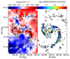 |
Fig. 16. Left: Torques per unit mass from Querejeta et al. (2016b) estimated from dust corrected (3.6 μm) Spitzer images. Right: HNCO(4–3)/CO(1–0) emission from SWAN (Stuber et al. 2025) for pixels where HNCO(4–3) is detected > 3σ. N2H+ contours are plotted on top. |
While this is a speculative explanation for non-linear behavior of the N2H+-bright spot, it does not explain the general offset of the ring environment compared to other environments. We find no global trends between average line ratios and torques, nor with average line intensity and torques.
6.4. Differences and similarities in northern versus southern spiral arm
M51 is known for an asymmetric behavior between northern and southern spiral arm likely induced by the dwarf companion galaxy M51b (e.g., Henry et al. 2003; Schinnerer et al. 2013). While the northern spiral arm shows prominent regions of high ΣSFR, the southern arm is rich in molecular gas emission (CO, HCN) but lacks high values of ΣSFR (see Fig. 1). Many literature studies have found the southern arm to be inefficient in forming stars (e.g., Querejeta et al. 2019). Querejeta et al. (2019) studied HCN at the same resolution in three pointings in M51 and when comparing peaks of HCN emission to the corresponding SFRs traced by 33 GHz emission, they find lower dense gas SFEs in the southern arm in contrast to the northern arm.
Our data, however, reveals that when averaging the northern disk and southern disk instead of focusing on bright spots only, the northern disk is overproducing stars, while the southern arm shows consistent behavior with the molecular ring and center. Per unit value of ΣSFR, all average line intensities of HCN, HNC, HCO+ and N2H+ are reduced in the northern disk compared to not only the southern disk, but also the center and ring environment (Appendix D). This overproduction seems independent of dense gas properties, as the dense gas line ratios as function of all physical properties agree between northern and southern disk (Fig. D.1). Thus while there are differences related to ΣSFR in the two spiral arms, the molecular gas chemistry might be more or less unaffected.
Potential explanations for these differences could include that the high SFR in the northern arm is destroying denser gas, thus reducing the average dense gas emission, whereas the southern arm, revealing high values of σCO, and high values of Pint/PDE (Fig. 14) is in a complex dynamical state.
7. Summary
We present observations of the J = 1-0 emission of HCN, HNC, HCO+, and N2H+ that traces the dense gas in the inner 5 × 7 kpc of the Whirlpool galaxy (M51) at 125 pc resolution from “Surveying the Whirlpool at Arcseconds with NOEMA” (SWAN). These observations cover very diverse environments, including spiral arms, a molecular ring, and the AGN affected center. We compare the emission of these molecules with each other, as well as with the surface densities of molecular gas mass (Σmol), SFR (ΣSFR), stellar mass (Σ*), and estimates of PDE and σCO, and find the following:
-
The average emission of HCN, HNC, HCO+, and N2H+ is generally correlated with each other. Average HCN, HNC, and HCO+ intensities follow N2H+ intensities, and so do HCN/CO, HNC/CO, and HCO+/CO ratios, but we find clear variations in slopes with galactic environments.
-
While average HCN, HNC, HCO+, and N2H+ are well correlated with Σmol, ΣSFR, Σ*, PDE, and σCO over several orders of magnitude, the slopes of these correlations vary from line to line and from environment to environment. The average N2H+ emission depends significantly more steeply on Σmol (slope of 1.48 ± 0.05) compared to HCN, HNC, and HCO+ (1.05 ± 0.04, 1.26 ± 0.02, 1.19 ± 0.03, respectively). The slope of the average HCN-to-Σmol relation is in agreement with the slope of the average CO-to-Σmol relation. Consequently, the HCN-, HNC-, and HCO+-to-N2H+ ratios are anticorrelated with Σmol. The different dependence of dense gas lines on Σmol could imply a different dependence on column densities as found in Milky Way studies, or it could stem from beam dilution effects.
-
The average HCN/CO, HNC/CO, HCO+/CO, and N2H+/CO relation shows a surprisingly shallow relation with Σmol, with slopes of the average HCN/CO-to-Σmol relation as low as 0.07 ± 0.03 and consistently shallower (or negative) in all environments compared to typical literature trends. While the N2H+/CO-to-Σmol relation is steeper (slope of 0.50 ± 0.05), large variations in the slopes across the environments can be found.
-
Dynamical equilibrium pressure, PDE, is a promising parameter well related to both dense gas emission and line ratios with CO, with smaller variations in slope across the environments compared to Σmol. We find indications of a PDE threshold, above which N2H+ emission is increased compared to HCN, HNC, and HCO+. Still, these CO line ratios have increased scatter when correlated with PDE compared to Σ* and ΣSFR.
-
Variations in line ratios can be seen from one environment to the other, and on cloud scales within individual environments. First, the nuclear outflow toward northeast of the center increases emission of HCN, HNC, and HCO+ compared to N2H+, and of all those lines compared to 12CO. Secondly, just outside the very center, within the ring, where we find an increased HCN/HCO+ ratio, the decreased ratio of internal to dynamical equilibrium pressure suggests that the clouds are not in balance with their environment. Thirdly, the molecular ring hosts the region with the brightest N2H+ emission, where gas flows might converge resulting in large-scale shocks. Lastly, we find asymmetries between the spiral arms. While the intensity pattern of all molecular lines as a function of ΣSFR in the northern arm deviates from those of all other environments, in the southern spiral arm we see enhanced velocity dispersion, enhanced Pint/PDE, and generally high quantities of bulk and dense molecular gas.
The cloud-scale relations of HCN, HNC, HCO+, and N2H+ across these environments in the inner disk of M51 reveal that while to first-order the molecules agree in their emission, when considering different environments and different physical properties, no two molecules have exactly the same emission pattern at those scales. Only SWAN can reveal these variations that occur on both larger-scale environments and on cloud scales within environments. In other galaxies, where the faint N2H+ emission is difficult to obtain and the conditions are similar to the conditions in the inner disk of M51, the emission of HCO+, which is nearly as bright as HCN, might be the favorable option to trace dense molecular gas.
Publicly available in the IRAM Data Management System https://oms.iram.fr/oms/?dms= or at the PAWS homepage https://www2.mpia-hd.mpg.de/PAWS/PAWS/Data.html
Acknowledgments
This work was carried out as part of the PHANGS collaboration and is based on data obtained by PIs E. Schinnerer and F. Bigiel with the IRAM-30 m telescope and NOEMA observatory under project ID M19AA. IRAM is supported by INSU/CNRS (France), MPG (Germany) and IGN (Spain) SKS thanks several PHANGS team members, specifically Adam Leroy for helpful discussions. SKS acknowledges financial support from the German Research Foundation (DFG) via Sino-German research grant SCHI 536/11-1. AU, MJD, and MQ acknowledge support from the Spanish grant PID2022-138560NB-I00, funded by MCIN/AEI/10.13039/501100011033/FEDER, EU. JPe acknowledges support by the French Agence Nationale de la Recherche through the DAOISM grant ANR-21-CE31-0010 and by the Thematic Action “Physique et Chimie du Milieu Interstellaire” (PCMI) of INSU Programme National “Astro”, with contributions from CNRS Physique & CNRS Chimie, CEA, and CNES. JS acknowledges support by the National Aeronautics and Space Administration (NASA) through the NASA Hubble Fellowship grant HST-HF2-51544 awarded by the Space Telescope Science Institute (STScI), which is operated by the Association of Universities for Research in Astronomy, Inc., under contract NAS 5-26555. HAP acknowledges support from the National Science and Technology Council of Taiwan under grant 113-2112-M-032 -014 -MY3. J.d.B. acknowledges support from the Smithsonian Institution as Submillimeter Array (SMA) Fellow. SCOG and RSK acknowledge financial support from the European Research Council via the ERC Synergy Grant “ECOGAL” (project ID 855130), from the German Excellence Strategy via the Heidelberg Cluster of Excellence (EXC 2181 - 390900948) “STRUCTURES”, and from thebibliography German Ministry for Economic Affairs and Climate Action in project “MAINN” (funding ID 50OO2206). RSK also thanks the 2024/25 Class of Radcliffe Fellows for highly interesting and stimulating discussions.
References
- Aalto, S. 2005, IAU Symp, 231, 261 [Google Scholar]
- Aalto, S., Radford, S. J. E., Scoville, N. Z., & Sargent, A. I. 1997, ApJ, 475, L107 [NASA ADS] [CrossRef] [Google Scholar]
- Aalto, S., Polatidis, A. G., Hüttemeister, S., & Curran, S. J. 2002, A&A, 381, 783 [NASA ADS] [CrossRef] [EDP Sciences] [Google Scholar]
- Aalto, S., Garcia-Burillo, S., Muller, S., et al. 2012, A&A, 537, A44 [NASA ADS] [CrossRef] [EDP Sciences] [Google Scholar]
- Aalto, S., Garcia-Burillo, S., Muller, S., et al. 2015, A&A, 574, A85 [NASA ADS] [CrossRef] [EDP Sciences] [Google Scholar]
- Aalto, S., Falstad, N., Muller, S., et al. 2020, A&A, 640, A104 [EDP Sciences] [Google Scholar]
- Backus, C., Velusamy, T., Thompson, T., & Arballo, J. 2005, ASP Conf. Ser., 347, 61 [Google Scholar]
- Barnes, A. T., Kauffmann, J., Bigiel, F., et al. 2020, MNRAS, 497, 1972 [NASA ADS] [CrossRef] [Google Scholar]
- Bemis, A., & Wilson, C. D. 2019, AJ, 157, 131 [NASA ADS] [CrossRef] [Google Scholar]
- Bešlic, I., Barnes, A. T., Bigiel, F., et al. 2021, MNRAS, 506, 963 [CrossRef] [Google Scholar]
- Bigiel, F., Leroy, A. K., Jiménez-Donaire, M. J., et al. 2016, ApJ, 822, L26 [NASA ADS] [CrossRef] [Google Scholar]
- Bolatto, A. D., Wolfire, M., & Leroy, A. K. 2013, ARA&A, 51, 207 [CrossRef] [Google Scholar]
- Chen, H., Braine, J., Gao, Y., Koda, J., & Gu, Q. 2017, ApJ, 836, 101 [NASA ADS] [CrossRef] [Google Scholar]
- Colombo, D., Hughes, A., Schinnerer, E., et al. 2014a, ApJ, 784, 3 [NASA ADS] [CrossRef] [Google Scholar]
- Colombo, D., Meidt, S. E., Schinnerer, E., et al. 2014b, ApJ, 784, 4 [Google Scholar]
- Croxall, K. V., Pogge, R. W., Berg, D. A., Skillman, E. D., & Moustakas, J. 2015, ApJ, 808, 42 [NASA ADS] [CrossRef] [Google Scholar]
- de Vaucouleurs, G., de Vaucouleurs, A., Corwin, Jr., H. G., et al. 1991, Third Reference Catalogue of Bright Galaxies (New York, NY (USA): Springer) [Google Scholar]
- den Brok, J. S., Bigiel, F., Sliwa, K., et al. 2022, A&A, 662, A89 [CrossRef] [EDP Sciences] [Google Scholar]
- den Brok, J., Jiménez-Donaire, M. J., Leroy, A., et al. 2025, AJ, 169, 18 [Google Scholar]
- Dumas, G., Schinnerer, E., Tabatabaei, F. S., et al. 2011, AJ, 141, 41 [NASA ADS] [CrossRef] [Google Scholar]
- Egusa, F., Mentuch Cooper, E., Koda, J., & Baba, J. 2017, MNRAS, 465, 460 [Google Scholar]
- Eibensteiner, C., Barnes, A. T., Bigiel, F., et al. 2022, A&A, 659, A173 [CrossRef] [EDP Sciences] [Google Scholar]
- Elmegreen, B. G. 1989, ApJ, 338, 178 [NASA ADS] [CrossRef] [Google Scholar]
- Evans, N. J., II, Heiderman, A., & Vutisalchavakul, N. 2014, ApJ, 782, 114 [CrossRef] [Google Scholar]
- Faustino Vieira, H., Duarte-Cabral, A., Davis, T. A., et al. 2024, MNRAS, 527, 3639 [Google Scholar]
- Field, G. B., Blackman, E. G., & Keto, E. R. 2011, MNRAS, 416, 710 [NASA ADS] [Google Scholar]
- Gallagher, M. J., Leroy, A. K., Bigiel, F., et al. 2018, ApJ, 858, 90 [NASA ADS] [CrossRef] [Google Scholar]
- Gao, Y., & Solomon, P. M. 2004, ApJ, 606, 271 [NASA ADS] [CrossRef] [Google Scholar]
- García-Burillo, S., Combes, F., Usero, A., et al. 2014, A&A, 567, A125 [Google Scholar]
- Gildas, T. 2013, Astrophysics Source Code Library [ascl:1305.010] [Google Scholar]
- Goldsmith, P. F., & Kauffmann, J. 2017, ApJ, 841, 25 [Google Scholar]
- Hacar, A., Bosman, A. D., & van Dishoeck, E. F. 2020, A&A, 635, A4 [NASA ADS] [CrossRef] [EDP Sciences] [Google Scholar]
- Harada, N., Nishimura, Y., Watanabe, Y., et al. 2019, ApJ, 871, 238 [NASA ADS] [CrossRef] [Google Scholar]
- Harada, N., Saito, T., Nishimura, Y., Watanabe, Y., & Sakamoto, K. 2024, ApJ, 969, 82 [Google Scholar]
- Helfer, T. T., & Blitz, L. 1993, ApJ, 419, 86 [NASA ADS] [CrossRef] [Google Scholar]
- Henry, A. L., Quillen, A. C., & Gutermuth, R. 2003, AJ, 126, 2831 [NASA ADS] [CrossRef] [Google Scholar]
- Heyer, M. H., Carpenter, J. M., & Snell, R. L. 2001, ApJ, 551, 852 [NASA ADS] [CrossRef] [Google Scholar]
- Ho, L. C., Filippenko, A. V., & Sargent, W. L. W. 1997, ApJS, 112, 315 [NASA ADS] [CrossRef] [Google Scholar]
- Imanishi, M., Baba, S., Nakanishi, K., & Izumi, T. 2023, ApJ, 950, 75 [NASA ADS] [CrossRef] [Google Scholar]
- Indriolo, N., Neufeld, D. A., Gerin, M., et al. 2015, ApJ, 800, 40 [NASA ADS] [CrossRef] [Google Scholar]
- Jiménez-Donaire, M. J., Bigiel, F., Leroy, A. K., et al. 2019, ApJ, 880, 127 [CrossRef] [Google Scholar]
- Jiménez-Donaire, M. J., Usero, A., Bešlić, I., et al. 2023, A&A, 676, L11 [NASA ADS] [CrossRef] [EDP Sciences] [Google Scholar]
- Jones, G. H., Clark, P. C., Glover, S. C. O., & Hacar, A. 2023, MNRAS, 520, 1005 [NASA ADS] [CrossRef] [Google Scholar]
- Jørgensen, J. K., Schöier, F. L., & van Dishoeck, E. F. 2004, A&A, 416, 603 [Google Scholar]
- Kauffmann, J., Goldsmith, P. F., Melnick, G., et al. 2017, A&A, 605, L5 [NASA ADS] [CrossRef] [EDP Sciences] [Google Scholar]
- Kessler, S., Leroy, A., Querejeta, M., et al. 2020, ApJ, 892, 23 [NASA ADS] [CrossRef] [Google Scholar]
- Klessen, R. S., & Glover, S. C. O. 2015, in Lessons from the Local Group: A Conference in honor of David Block and Bruce Elmegreen, eds. K. Freeman, B. Elmegreen, D. Block, & M. Woolway, 137 [Google Scholar]
- Koda, J., Sawada, T., Wright, M. C. H., et al. 2011, ApJS, 193, 19 [NASA ADS] [CrossRef] [Google Scholar]
- Kohno, K. 2005, Am. Inst. Phys. Conf. Ser., 783, 203 [Google Scholar]
- Kregel, M., van der Kruit, P. C., & de Grijs, R. 2002, MNRAS, 334, 646 [NASA ADS] [CrossRef] [Google Scholar]
- Krieger, N., Bolatto, A. D., Leroy, A. K., et al. 2020, ApJ, 897, 176 [Google Scholar]
- Krolik, J. H., & Kallman, T. R. 1983, ApJ, 267, 610 [Google Scholar]
- Krumholz, M. R. 2014, Phys. Rep., 539, 49 [Google Scholar]
- Lada, C. J., Forbrich, J., Lombardi, M., & Alves, J. F. 2012, ApJ, 745, 190 [NASA ADS] [CrossRef] [Google Scholar]
- Lamers, H. J. G. L. M., Panagia, N., Scuderi, S., et al. 2002, ApJ, 566, 818 [NASA ADS] [CrossRef] [Google Scholar]
- Le Petit, F., Ruaud, M., Bron, E., et al. 2016, A&A, 585, A105 [NASA ADS] [CrossRef] [EDP Sciences] [Google Scholar]
- Leroy, A. K., Walter, F., Sandstrom, K., et al. 2013, AJ, 146, 19 [Google Scholar]
- Leroy, A. K., Schinnerer, E., Hughes, A., et al. 2017a, ApJ, 846, 71 [Google Scholar]
- Leroy, A. K., Usero, A., Schruba, A., et al. 2017b, ApJ, 835, 217 [NASA ADS] [CrossRef] [Google Scholar]
- Leroy, A. K., Hughes, A., Liu, D., et al. 2021a, ApJS, 255, 19 [NASA ADS] [CrossRef] [Google Scholar]
- Leroy, A. K., Schinnerer, E., Hughes, A., et al. 2021b, ApJS, 257, 43 [NASA ADS] [CrossRef] [Google Scholar]
- Maloney, P. R., Hollenbach, D. J., & Tielens, A. G. G. M. 1996, ApJ, 466, 561 [Google Scholar]
- Martín, S., Mangum, J. G., Harada, N., et al. 2021, A&A, 656, A46 [NASA ADS] [CrossRef] [EDP Sciences] [Google Scholar]
- Matsushita, S., Trung, D.-V., Boone, F., et al. 2015, ApJ, 799, 26 [NASA ADS] [CrossRef] [Google Scholar]
- McQuinn, K. B. W., Skillman, E. D., Dolphin, A. E., Berg, D., & Kennicutt, R. 2016, ApJ, 826, 21 [NASA ADS] [CrossRef] [Google Scholar]
- Meidt, S. E., Schinnerer, E., García-Burillo, S., et al. 2013, ApJ, 779, 45 [NASA ADS] [CrossRef] [Google Scholar]
- Meier, D. S., & Turner, J. L. 2005, ApJ, 618, 259 [NASA ADS] [CrossRef] [Google Scholar]
- Meier, D. S., Walter, F., Bolatto, A. D., et al. 2015, ApJ, 801, 63 [NASA ADS] [CrossRef] [Google Scholar]
- Mills, E. A. C., & Battersby, C. 2017, ApJ, 835, 76 [NASA ADS] [CrossRef] [Google Scholar]
- Nakajima, T., Takano, S., Tosaki, T., et al. 2023, ApJ, 955, 27 [NASA ADS] [CrossRef] [Google Scholar]
- Neumann, L., Gallagher, M. J., Bigiel, F., et al. 2023a, MNRAS, 521, 3348 [NASA ADS] [CrossRef] [Google Scholar]
- Neumann, L., den Brok, J. S., Bigiel, F., et al. 2023b, A&A, 675, A104 [NASA ADS] [CrossRef] [EDP Sciences] [Google Scholar]
- Neumann, L., Bigiel, F., Barnes, A. T., et al. 2024, A&A, 691, A121 [NASA ADS] [CrossRef] [EDP Sciences] [Google Scholar]
- Neumann, L., Jiménez-Donaire, M. J., Leroy, A. K., et al. 2025, A&A, 693, L13 [NASA ADS] [CrossRef] [EDP Sciences] [Google Scholar]
- Oka, T., Geballe, T. R., Goto, M., et al. 2019, ApJ, 883, 54 [Google Scholar]
- Ostriker, E. C., & Kim, C.-G. 2022, ApJ, 936, 137 [NASA ADS] [CrossRef] [Google Scholar]
- Ostriker, E. C., McKee, C. F., & Leroy, A. K. 2010, ApJ, 721, 975 [CrossRef] [Google Scholar]
- Papadopoulos, P. P. 2007, ApJ, 656, 792 [NASA ADS] [CrossRef] [Google Scholar]
- Pety, J., Guzmán, V. V., Orkisz, J. H., et al. 2017, A&A, 599, A98 [NASA ADS] [CrossRef] [EDP Sciences] [Google Scholar]
- Priestley, F. D., Clark, P. C., Glover, S. C. O., et al. 2023, MNRAS, 526, 4952 [NASA ADS] [CrossRef] [Google Scholar]
- Priestley, F. D., Clark, P. C., Glover, S. C. O., et al. 2024, MNRAS, 531, 4408 [NASA ADS] [CrossRef] [Google Scholar]
- Querejeta, M., Meidt, S. E., Schinnerer, E., et al. 2015, ApJS, 219, 5 [NASA ADS] [CrossRef] [Google Scholar]
- Querejeta, M., Schinnerer, E., García-Burillo, S., et al. 2016a, A&A, 593, A118 [NASA ADS] [CrossRef] [EDP Sciences] [Google Scholar]
- Querejeta, M., Meidt, S. E., Schinnerer, E., et al. 2016b, A&A, 588, A33 [NASA ADS] [CrossRef] [EDP Sciences] [Google Scholar]
- Querejeta, M., Schinnerer, E., Schruba, A., et al. 2019, A&A, 625, A19 [NASA ADS] [CrossRef] [EDP Sciences] [Google Scholar]
- Rosolowsky, E., & Leroy, A. 2006, PASP, 118, 590 [NASA ADS] [CrossRef] [Google Scholar]
- Sage, L. J., & Ziurys, L. M. 1995, ApJ, 447, 625 [NASA ADS] [CrossRef] [Google Scholar]
- Santa-Maria, M. G., Goicoechea, J. R., Pety, J., et al. 2023, A&A, 679, A4 [NASA ADS] [CrossRef] [EDP Sciences] [Google Scholar]
- Schinnerer, E., & Leroy, A. K. 2024, ARA&A, 62, 369 [NASA ADS] [CrossRef] [Google Scholar]
- Schinnerer, E., Meidt, S. E., Pety, J., et al. 2013, ApJ, 779, 42 [Google Scholar]
- Schober, J., Schleicher, D. R. G., & Klessen, R. S. 2015, MNRAS, 446, 2 [Google Scholar]
- Sheth, K., Regan, M., Hinz, J. L., et al. 2010, PASP, 122, 1397 [Google Scholar]
- Shetty, R., Vogel, S. N., Ostriker, E. C., & Teuben, P. J. 2007, ApJ, 665, 1138 [NASA ADS] [CrossRef] [Google Scholar]
- Stuber, S. K., Pety, J., Schinnerer, E., et al. 2023, A&A, 680, L20 [NASA ADS] [CrossRef] [EDP Sciences] [Google Scholar]
- Stuber, S., Pety, J., Usero, A., et al. 2025, A&A, 696, A182 [NASA ADS] [CrossRef] [EDP Sciences] [Google Scholar]
- Sun, J., Leroy, A. K., Schruba, A., et al. 2018, ApJ, 860, 172 [NASA ADS] [CrossRef] [Google Scholar]
- Sun, J., Leroy, A. K., Ostriker, E. C., et al. 2020, ApJ, 892, 148 [NASA ADS] [CrossRef] [Google Scholar]
- Sun, J., Leroy, A. K., Rosolowsky, E., et al. 2022, AJ, 164, 43 [NASA ADS] [CrossRef] [Google Scholar]
- Tafalla, M., Santiago-García, J., Hacar, A., & Bachiller, R. 2010, A&A, 522, A91 [CrossRef] [EDP Sciences] [Google Scholar]
- Tafalla, M., Usero, A., & Hacar, A. 2021, A&A, 646, A97 [NASA ADS] [CrossRef] [EDP Sciences] [Google Scholar]
- Tafalla, M., Usero, A., & Hacar, A. 2023, A&A, 679, A112 [NASA ADS] [CrossRef] [EDP Sciences] [Google Scholar]
- Usero, A., García-Burillo, S., Fuente, A., Martín-Pintado, J., & Rodríguez-Fernández, N. J. 2004, A&A, 419, 897 [NASA ADS] [CrossRef] [EDP Sciences] [Google Scholar]
- Usero, A., Leroy, A. K., Walter, F., et al. 2015, AJ, 150, 115 [Google Scholar]
- Watanabe, Y., Sakai, N., Sorai, K., & Yamamoto, S. 2014, ApJ, 788, 4 [NASA ADS] [CrossRef] [Google Scholar]
- Wu, J., Evans, N. J. II, Gao, Y., et al. 2005, ApJ, 635, L173 [NASA ADS] [CrossRef] [Google Scholar]
- Zhang, C., Wang, J., & Cao, T.-W. 2025, ApJ, 978, L15 [Google Scholar]
Appendix A: Mock data to test the effect of low S/N
Comparing the emission of molecular lines with different intrinsic intensities in datasets with similar noise levels is challenging, as fainter emission lines (such as N2H+(1–0)) are much more strongly affected by noise, resulting in a lower fraction of significant detections than brighter lines. Including/excluding regions based on their S/N alone can thus bias any measurement of lines of different brightness differently. To address this issue, we simulate the effect of different brightness levels using the CO(1–0) data cube, which contains a lot of signal compared to its noise level with significant detections across most of our FoV. We present the methodology to generate data cubes representing fainter lines (Appendix A.1), and create moment-maps. We explore different commonly used approaches to determine average intensities and line ratios based on the mock-data in Appendix A.2. Since the noise in observations averages to zero, binning is commonly used to recover relations. We test the effect on binning on our mock datasets inAppendix A.3.
A.1. Creation of mock datasets
We take the CO(1–0) data cube from PAWS matched to the SWAN data at 3″ resolution with a spectral resolution of 10 km/s (see Sect. 2.3.2). First, we scale the intensity of the CO data cube by a constant line ratio S. This factor represents the true line ratio we want to recover in our analysis. We call this scaled data cube A. Next, we create a data cube filled with only simulated noise. At each pixel and for each channel we randomly draw values from a Gaussian distribution with arbitrary amplitude. We then spatially convolve the Gaussian noise for each channel of the noise cube by our beam size of 3″. This will correlate the noise of neighboring pixels as it is the case for our interferometric observations from SWAN. While technically the noise is not just correlated across a beam, but across larger scales as well, this is not included in this simple test. The amplitude of the correlated noise in the noise data cube is scaled to match an RMS of 8.6 mK which corresponds to the RMS of N2H+ from our SWAN observations (Stuber et al. 2025). Lastly, we add the cube containing the correlated scaled noise to the scaled CO data cube A. We do not add the cube in quadrature, as the relative noise in the scaled CO cube is negligible compared to the noise added. This final data cube is our”mock-data cube”.
We perform these steps with line ratios of S = 0.024, 0.016, 0.007, 0.0036. The noise cube is drawn anew for each S. Those are line ratios obtained from different methods to calculate the N2H+-to-CO line ratio within the literature (i.e., see Jiménez-Donaire et al. 2023; Schinnerer & Leroy 2024). Those values further roughly match our typical HCO+-to-12CO, HNC-to-12CO and N2H+-to-12CO line ratios (0.033, 0.018, 0.008, Table 2) with an additional even smaller line ratio to account for individual regions (i.e. norhtern disk) with increasednoise.
Our measurements of the observed SWAN line emission (Sect. 4 and following) is not performed on the data cubes directly, but on the moment maps (Sect. 2.2). Therefore, we create a PyStructure based on the exact same criteria as before (using HCN and CO as priors, Sect. 2.2), integrating the Mock data cubes. The resulting moment-0 maps are shown in Fig. A.1. We add the moment-0 map of N2H+(1–0), the faintest of the dense gas tracing lines, forcomparison.
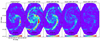 |
Fig. A.1. Integrated emission of N2H+(1–0) and Mock data cubes based on the original CO(1–0) data cube, scaled down by a line ratio of (from left to right) LR = 41,62,142,277 and adding noise to simulate lower S/N observations. |
A.2. Recovering average intensity ratios
We compare different methods to recover average line ratios between our mock-data and the original 12CO data in Fig. A.2. These methods are the mean and median line ratio of all pixels, as well as the integrated intensity of the mock data divided by the integrated CO data (sum(M)/sum(CO) = Σimock / ΣiCO). We apply these methods to a) the full FoV, excluding the edges where the noise is increased (see Stuber et al. 2025), b) a ICO-based mask and c) a Imock-based mask. The ICO (Imock) mask exclude pixels in which the CO (mock) intensity is below 3σ. In Fig. A.2 we show the relative difference between the measured line ratio and the true line ratio (LRtrue) used in the generation of the mock cubes.
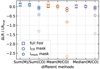 |
Fig. A.2. Testing different methods to calculate CO line ratios and the effect of masking. We show the relative difference between the true and measured line ratio ΔLR/LRtrue with ΔLR=LRtrue - LRmeasured. We estimate the measured line ratio LRmeasured per three different methods (sum: sum(M)/sum(CO) in blue, mean: mean(M/CO) in orange, median: median(mock/CO) in purple) with M and CO indicating the intensity of the mock and CO data, respectively. We further test the impact of different masking on the moment maps: Utilizing all pixels in the FoV (squares), only pixels where CO is significantly detected (> 3σ, circle), and only pixels where N2H+ is significantly detected (> 3σ, pentagons). The color gradient indicates the S/N of the data cube (measured via LRtrue), with darker color being LRtrue = 0.024 and the faintest color LRtrue = 0.0036. Points of the same color (albeit different gradient) belong to the same method. |
The deviations between measured and true line ratio between different methods are small compared to the deviations between different masking techniques. The largest deviations occur when applying the Imock-based mask. The smaller the true CO-line ratio (the smaller the S/N), the larger the deviation due to masking. The Imock-based mask is biased toward fewer and brighter pixels compared to the other masks. This will result in a bias toward more positive measurements.
The difference between values derived using the full FoV and within the ICO-based mask is small as expected. As the moment-0 maps are created using CO and HCN emission as a prior, there are only few pixels within the resulting moment-0 map where the integrated 12CO emission is less than 3 times its corresponding value.
We test the calculation of line ratios between the mock data, that are all much fainter than the CO line, in Fig. A.3. Similar to before we test both different calculation methods, and different masking techniques. We find the sum-method (integrated intensity of mock1 divided by integrated intensity of mock2) results in the most reliable results, even for large true line ratios. This method is also least effected by masking.
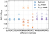 |
Fig. A.3. Testing the effect of masking on different methods to calculate average line ratios of mock-data. Same as Fig. A.2 but for line ratios between different mock datasets. The color gradient indicates the expected line ratio (measured via LRtrue). The ratio of Mock41 and Mock227 results in the largest line ratio (and thus faintest data point). Two outliers with large ΔLR/LRtrue are only shown as lower limits (colored triangle). |
A.3. Binning mock data intensities and ratios
When measuring relations between molecular line emission and other parameters such as, for example, galactocentric radius or molecular gas surface density, binning the emission (also known as averaging the emission in increments of, e.g., galactocentric radius) is a commonly used technique to recover the physical relation that is obscured by noise. Ideally, the noise (including positive and negative noise values) in each bin will average to zero and the actual signal can be recovered. We test how well binning recovers the known relation between our mock data and the 12CO data in Fig. A.4. The binning method used is described in Sect. 3.2. The true relation is very well recovered when all data points are used. Masking pixels (> 3σ) results in a flattening of the average relation for low CO intensities.
Fitting those masked and unmasked binned line ratios (Sect. 3.2) confirms this bias: When using all data, we can recover the true relation (slope of 1) in all of the mock datasets, even in the data with lowest S/N (LR = 277). When restricting the data to > 3σ, slopes are artificially decreased with decreasing average S/N of the mock data and significantly deviate from the true slope of unity.
In addition to binning line intensities, we test if we are able to recover the relation between line ratios and other more independent parameters, such as molecular gas, star-formation rate and stellar mass surface densities, galactocentric radius, velocity dispersion and dynamical equilibrium pressure used in our analysis (Sect. 5). Figure A.5 shows the binned mock-to-CO line ratios as function of those parameters. We expect a flat relation (slope 0) with different offsets along the y-axis depending on the mock data used.
Most mock-to-CO line ratios are flat as expected (Fig. A.5). Again, masking pixels < 3σ introduces significant biases and results in artificial slopes that are largest for the mock data with the lowest S/N. This bias is strongest for relations of line ratios with Σmol, σCO and PDE, with a > 5σ deviation of slopes obtained from the lowest S/N mock data (LR = 277) to the true slope of zero. When including all data, we can recover the expected slope of zero for all mock datasets as function of all galactic parameters.
This simple mock dataset is not a perfect representation of the actual noise, as it does not consider noise correlated over scales larger than a beam-size. Still, it shows the impact of excluding parts of the data on the ability to retrieve the correct result. The actual correlations shown might suffer from additional noise sources not considered in this mock dataset.
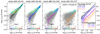 |
Fig. A.4. Testing the effect of binning to recover average line relations. We show the intensity of each pixel in the mock-moment-0 map (Imock) as function of the correponding intensity in the 12CO moment-0 map (ICO. The different mock data are simulated based on 12CO data scaled by a line ratio of 0.024, 0.016, 0.007, 0.0036 (aka LR: 41, 62, 142, 277). The expected relation (black dashed line) corresponds to line ratio used to create the mock data (power of 1, offset corresponds to the line ratio). We highlight pixels where Imock is significantly detected (>3σ, colored data points) and indicate their galactocentric distance by color. We bin Imock in logarithmic steps of ICO for all pixels in the FoV (solid line), as well as when only including pixels with significant detections (dotted line). We add the slopes of linear fits fitted to the binned data for the full FoV and the masked data. |
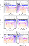 |
Fig. A.5. Binned mock-to-CO line ratios as function of physical parameters such as molecular gas mass, stellar mass and SFR surface densities, velocity dispersion, galactocentric radius and dynamical equilibrium pressure. We show the binned line ratios using all pixels (solid line), as well as restricting to detections (intensity >3σ, dotted lines). |
A.4. Estimating the scatter of mock data relations
The scatter of a relation between line emission and physical parameters is equally important in assessing the strength of the relation as the slope. As an example, if the relation between line intensity and two galactic properties show similar slopes, increased scatter in one may suggest a secondary dependence on other factors. Unfortunately, a lower S/N coincides with an increased scatter, which challenges the interpretation of the scatter calculated using the line emission of lines of different average S/N. We test this impact of S/N on the calculation of the scatter with our mock data and galactic parameters. Figure A.6 shows the average scatter of mock line intensities as function of physical galactic properties. The scatter is the medium absolute deviation of the line intensity as function of galactic properties after subtracting a linear relation fitted to the binned intensities (Sect. 3.2). Per galactic quantity, the maximum deviation in scatter from different mock datasets ranges from 0.2 dex (relations with PDE, Σmol) to 0.5 dex (σCO, Σ*, dist). The variations in scatter between the different galactic quantities is expected, as some quantities (Σmol, PDE) depend on the 12CO intensity, which is the basis for the mock dataset.
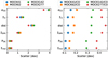 |
Fig. A.6. Average scatter of mock intensity (left panel) and mock-to-CO line ratios (left panel) as function of galactic physical properties tested for different mock datasets (Mock41-Mock277). |
In addition to line intensity, we test the scatter of relations between mock-to-12CO line ratios and galactic physical properties in Fig. A.6. For each galactic property, the average scatter increases significantly with decreasing average S/N (lowest S/N for mock277), as expected. For each mock dataset, variations in the mock-to-CO relation with different galactic properties are small: We find the least variations in scatter across galactic properties for the highest S/N dataset (mock41, scatter varies by ∼0.04, followed by ∼0.06, ∼0.06, ∼0.08 for mock62, mock142 and mock277 respectively.) These variations in the average scatter are driven by the varying S/N and different sorting due to the galactic parameters.
Appendix B: Testing different prescriptions of Σmol
We test the performance of the average HCN-to-12CO line ratio when comparing to different prescriptions of calculating Σmol in Fig. B.1 The methods to calculate Σmol are described below.
A common method to estimate the CO-to-H2 conversion factors is via the metallicity and stellar mass surface density in the disk, which we refer to as  . We first obtain the αCO distribution based on radial metallicity profiles from CHAOS (Croxall et al. 2015). These are converted into αCO values according to the prescription in Bolatto et al. (2013), which relies not only on the metallicity but also on the kiloparsec-scale surface density of stellar mass, atomic gas and molecular gas. The values were calculated iteratively as described in Sun et al. (2022). Inside the SWAN FoV, αCO has a median of 1.99 M⊙ (K km s−1 pc−2)−1, with 16th and 84th percentiles of 1.35, 2.75 M⊙ (K km s−1 pc−2)−1, respectively. It also has a strong radial gradient: the central 1 kpc (diameter) median αCO is 0.72 M⊙ (K km s−1 pc−2)−1, the median αCO at galactocentric distance larger than 3 kpc is 2.81 M⊙ (K km s−1 pc−2)−1.
We add our first prescription, using a measured αCO that is applied to the integrated 12CO intensities (see Sect. 2.3.2). We refer to this surface density as Σmolmeasured.
If the αCO value is not known precisely, a common method is to assume a constant based on Galactic measurements (Bolatto et al. 2013). Commonly used in extragalactic targets is a value of αCO = 4.35M⊙ (K km s−1 pc−2)−1. We calculate the gas surface density by applying this constant conversion factor to the 12CO moment-0 map. We refer to this surface density as Σmolconst.
Lastly, we add measurements of gas surface density from Faustino Vieira et al. (2024) based on HST observations for comparison. We refer to this surface density as  .
.
While there are difference in the average HCN/CO ratio as function of those different values of Σmol, we note that most of them are similar, comparably flat, or even result in negative trends ( ). The relation obtained using a constant CO-to-H2 conversion factor reveals the steepest relation, but we note, that a constant value of αCO is not able to reflect the changes expected in environment, such as a generally increased αCO in galaxy centers (Schinnerer & Leroy 2024).
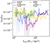 |
Fig. B.1. Average HCN/CO line ratio as function of Σmol, with Σmol being calculated with four different methods: a) a constant αCO conversion factor multiplied to 12CO emission (Σmolconst) b) the measured αCO as described in Sect. 2.3.2, Σmolmeasured c) a metallicity and stellar mass based αCO, |


Appendix C: The impact of the central environment on the average HCN/CO to Σmol relation
We test the effect of the central pixels on the performance of the HCN/CO-to-Σmol relation by removing central apertures of increasing sizes in Fig. C.1. Further, we fit the binned HCN/CO-to-Σmol relations and provide fit slopes in Table C.1. We add Spearman correlation coefficients (ρSp) for the respective apertures in Table C.1. We note that ρSp is sensitive to the S/N of the line, therefore we expect brighter lines to have higher values of ρSp.
While we can see an increase in the slopes of the HCN/CO-to-Σmol relation with increasing aperture that is removed from the analysis, the values stay overall small. At a radius of ∼1 kpc the molecular ring is reached. Figure C.1 shows that particularly pixels at intermediate values of Σmol are removed when excluding central apertures of increasing sizes. The molecular outflow driven by the AGN is most prominent in a small region with the size of ∼200 pc in the center (Querejeta et al. 2016a). The actual impact of the AGN on the molecular gas, however, is under discussion (Querejeta et al. 2016a, 2019; Zhang et al. 2025, see also Sect. 6) and some effects might reach out to radii of ∼600 pc north of the AGN. The slopes of the HCN/CO-to-Σmol relation however, show a continuous increase with increased size of the excluded aperture. The HCN/CO ratio as function of Σmol reaches a slope of up to 0.36 ± 0.02. Spearman correlation coefficients do not change even when excluding the central 1 kpc in radius. In all cases values of ρSp are highest for the HCO+/CO ratio as function of Σmol, despite HCN being on average brighter than HCO+.
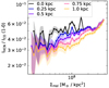 |
Fig. C.1. Average HCN/CO line ratio as function of Σmol when excluding pixels inside the central r = 0, 0.25, 0.5, 0.75, and 1 kpc in radius. The ratio is binned as described in Sect. 3.2 and we use the same values of Σmol, that we use in the main text. |
Fitting CO line ratios (LR) as function of Σmol when excluding central apertures of varying sizes
Appendix D: Environmental dependence of line emission and line ratios
Figure D.1 shows the average line intensities and average line ratios for all dense gas tracers as function of all environmental parameters tested for (Σmol, ΣSFR, Σ*, r, PDE, σCO) for different environments in the disk. The binning is the same as for Figs. 7 and 11), but for pixels inside the corresponding environment. No masking is applied for average line intensities and line ratios (compare Sect. 3.2). The center and ring environments are based on a kinematic analysis of Colombo et al. (2014b), and we additionally separate the disk into northern and southern parts based on the galaxy center, to test for asymmetries between the spiral arms. All environments are shown in Fig. 1.
For all molecules, the trend between line intensity and Σmol is offset to slightly higher line intensities in the center compared to the molecular ring and both northern and southern disk, which agree well. This is in agreement with the inverse radial dependence of the line emission found in Sect. 5.1. Similarly, there is an offset relation between average line intensity and σCO from one environment to the other, with the average line intensity being higher in center and ring compared to both spiral arms at the same values of σCO. Despite the offset, the shapes of the relations are very similar across all environments.
For ΣSFR, however, the opposite can be seen: Center, ring and southern disk agree on a single distribution of line intensity as function of ΣSFR, but the northern disk depends more shallow on ΣSFR. While the line ratios differ for the center environment as function of ΣSFR, the line ratios of the northern and southern arm mostly agree. The line ratios with N2H+ in the denominator are generally slightly lower in the southern arm compared to the northern one, but the data points agree well within their uncertainties.
Average line ratios among the dense gas tracing lines HCN, HNC, HCO+ and N2H+ generally show very similar behavior with galactic properties across the individual environment. The most remarkable difference seen is the relation betweeen line ratios with N2H+ and their dependence on Σmol. We explore those in more detail in the main text.
Fitting average line intensities as function of physical properties per environment
Fitting average CO line ratios as function of galactic physical properties per environment
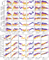 |
Fig. D.1. Average line ratios (top panels) and average line intensities (bottom panels) and as function of Σmol, ΣSFR, r, Σ*, σCO and PDE for different environments in the disk (see Fig. 1). |
Appendix E: Pixel-by-pixel distribution of line intensities and line ratios as function of galaxy properties
We show the pixel-by-pixel distribution of line intensities of HCN, HNC, N2H+ and HCO+ as function of galactic properties (Σmol, ΣSFR, Σ*, r, PDE, σCO) in Fig. E.1. The data is colored by galactocentric radius, so that the impact of the central pixels can be clearly seen in the intensity-to-Σmol relation: All of the tested lines have bright emission in the center, that follows a distribution offset from the rest of the data points.
Figure E.1 also shows the binned intensity trends utilizing all data points and only data points where emission is significantly detected. As discussed in Sect. 3.2 and Appendix A.3, excluding data points from the analysis can significantly bias the results.
We add Spearman correlation coefficients ρSp using all data (no masking) in Fig. E.1. These coefficients are strongly dependent on the S/N of the data and therefore we expect to find a decrease in coefficient value from brighter to fainter lines, or in our case, from HCN to N2H+. For each line we find ρSp highest for line intensity as function of PDE, followed by Σmol, ΣSFR, Σ*, r and σCO.
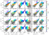 |
Fig. E.1. Pixel-by-pixel integrated line intensities for HCN, HNC, N2H+, HCO+(1–0) as function of Σmol, ΣSFR, Σ*, galactocentric radius, PDE and σCO for both detected emission (> 3σ, colored by galactocentric distance) as well as all data (gray). Pixels with detected emission are colored by galactocentric radius. We show the binned average for all data (black solid line) and significant data (black dashed line). We add Spearman correlation coefficients using all data in the top left corner of each panel, but note that those coefficients strongly depend on the S/N of the line and a decrease in coefficients from brighter to fainter lines is expected (i.e. from HCN to N2H+). All p-values are below 5%. |
Similarly, we show the pixel-by-pixel distribution of line intensities of HCN, HNC, N2H+ and HCO+ divided by 12CO emission as function of galactic properties (Σmol, ΣSFR, Σ*, r, PDE, σCO) in Fig. E.2. Lastly, we also show the pixel-by-pixel distribution of line ratios among the dense gas tracing lines in Fig. E.3.
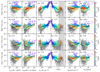 |
Fig. E.2. Same as Fig. E.1 but for 12CO line ratios. We mark Spearman correlation coefficients for which the corresponding p-value is below 5% with an asterisk. |
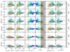 |
Fig. E.3. Same as Fig. E.1 but for line ratios between dense gas tracing lines HCN, HNC, HCO+ and N2H+. |
All Tables
Fitting average line intensities and average CO-line ratios as a function of N2H+ intensity or N2H+/CO ratio per environment.
Fitted slopes to binned line ratios as function of Σmol, ΣSFR, Σ*, PDE, σCO and radius.
Fitting CO line ratios (LR) as function of Σmol when excluding central apertures of varying sizes
Fitting average line intensities as function of physical properties per environment
Fitting average CO line ratios as function of galactic physical properties per environment
All Figures
|
Fig. 1. Integrated intensity maps of dense gas tracers HCN, HNC, HCO+, and N2H+ from SWAN at a common resolution of 3″ (top row from left to right), as well as from 12CO (PAWS, bottom left). We divide the disk into a center and ring environment (Colombo et al. 2014a), and the outer disk into northern and southern halves (bottom row, second panel from left). We add contours of integrated N2H+ emission of 0.75, 2, and 4 K km/s to the environment map. We show the pixel-based integrated intensity distribution (in Kelvin kilometer per seconds) in various environments in the disk for all pixels in the FoV (colored shaded area), as well as for pixels where emission is detected (emission > 3σ, light gray shaded area) in the bottom right panels. The area of each histogram is normalized to unity. We indicate the median of all pixels (black dashed line) and median of masked pixels (dotted gray line) of each environment. The median represents the median value of logarithmic emission (med(log10(I))). Pixels with negative emission are excluded in the logarithmic scaling of the histograms. Since CO is detected across most of the FoV and is used as a prior in the creation of the moment-0 map (Sect. 2.2), its masked histogram distribution agrees well with the unmasked one. |
| In the text | |
|
Fig. 2. Molecular gas mass surface densities, Σmol, star-formation rate surface densities, ΣSFR, stellar mass surface density, Σ*, dynamical equilibrium pressure, PDE, as well as CO velocity dispersion σCO at 3″ resolution. We show the contours of integrated N2H+ emission (0.75, 2,4 K km/s) on top. |
| In the text | |
|
Fig. 3. Left panel: Line ratios of integrated line emission from dense gas tracers HCN, HNC, and HCO+. For visual purposes, we only show line ratios for significant detected pixels (> 3σ), but include nondetections in all calculations. We mark pixels in which CO is detected (gray points) and the center of the galaxy (green plus). The intensity scale is centered logarithmically on the average line ratios (log10R, with R from Table 2) determined for all pixels in the FoV, including nondetections. The average line ratio (log10R) and the total range of 1 dex covered by the color bar are indicated by the dashed black line and gray shaded area in the right panel. We show contours of integrated N2H+ emission (0.75, 3 K km/s) on top. Right panel: Histogram of line ratios per environment analogous to Fig. 1 but for HCN/HNC, HCN/HCO+, and HNC/HCO+ (colored histograms). We indicate the number of pixels shown in the histogram (top right corner), which varies slightly, as values with negative noise cannot be shown in the logarithmic scale. |
| In the text | |
|
Fig. 4. Same as Fig. 3 but for the HCN-to-N2H+, HNC-to-N2H+, and HCO+-to-N2H+ line ratios. The colorbar spans the same 1 dex range as in Fig. 3, and is centered logarithmically on the average line ratios (log10R, with R from Table 2). |
| In the text | |
|
Fig. 5. Same as Figs. 3 and 4 but for line ratios with CO. In contrast to the previous figures, the colorbar spans a larger range of 1.5 dex, centered on the average line ratios (Table 2), and we add line ratios in pixels with nondetections. Since we show the logarithmic line ratio, negative values that arise from negative noise cannot be shown in either the spatial map or the histograms. We mark pixels where CO is significantly detected, but the line ratio cannot be shown in logarithmic scaling in dark gray. The contours depict integrated N2H+ emission at 0.75 and 3 K km/s. |
| In the text | |
|
Fig. 6. Average intensities of HCN, HNC, and HCO+ as function of N2H+ intensity (left) as well as average 12CO line ratios of HCN, HNC, and HCO+ (right) as function of the N2H+/CO line ratio emission. We do not apply any masking, but utilize all pixels in the FoV. We show the binned intensities and binned line ratios for the total FoV (top) as well as for individual environments (Fig. 1). We provide lines of constant slopes in log space for visual guidance (dashed black lines). The bins cover a range between three times the average N2H+ (N2H+/CO) uncertainty up to the maximum N2H+ intensity (N2H+/CO line ratio). |
| In the text | |
|
Fig. 7. Average line intensity, ILine, as a function of surface densities of molecular gas mass (Σmol), stellar mass (Σ*), and star-formation rate (ΣSFR), as well as velocity dispersion (σCO), dynamical equilibrium pressure (PDE), and galactocentric radius for all dense gas tracers. Shaded areas mark the standard deviation per bin. The 12CO intensity scaled by a factor of 1/10 is added for comparison (gray line). For r > 2.2 kpc, the shape of our FoV leads to incomplete sampling of these radial bins (gray shaded area). The obtained slopes for a linear fit (in log space) to the binned averages are provided in each panel. |
| In the text | |
|
Fig. 8. Average scatter of dense gas line intensity (left panel) and average dense gas to CO line ratios (right panel) as a function of physical galactic properties with respect to a linear relation (methodology described in Sect. 3.2). The impact of S/N on this plot is shown in Appendix A.4. |
| In the text | |
|
Fig. 9. Spearman correlation coefficients of line intensity (left panel) and average dense gas to CO line ratios (right panel) as a function of physical galactic properties (Sect. 2.3). An increased S/N will directly result in a lower correlation coefficient. We therefore expect higher correlation coefficients for HCN, followed by HCO+, then HNC, then N2H+ as a function of the same galactic properties. All p values are below 5% except p values for the line/CO ratios as a function of σCO. |
| In the text | |
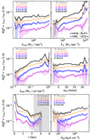 |
Fig. 10. Same as Fig. 7 but for line ratios with 12CO. |
| In the text | |
|
Fig. 11. Average line ratios of HCN/HNC, HCN/HCO+ and HNC/HCO+ (left panels) as function of physical properties as well as for HCN/N2H+, HNC/N2H+, HCO+/N2H+ (right panels). Error bars depict the 25/75th percentiles. |
| In the text | |
|
Fig. 12. Same as right panels of Fig. 11, but only for relations with Σmol and separated into the different environments. We note that fitting the binned averages as function of Σmol results in slopes that are within 5σ to a slope of zero for all line ratios as function of Σmol, except for the ring environment, where the slopes are significantly negative. The slopes for the HCN-, HNC- and HCO+-to-N2H+ line ratio as function of Σmol in the ring environment are −0.63 ± 0.04, −0.48 ± 0.04 and −0.46 ± 0.04, respectively. |
| In the text | |
|
Fig. 13. Literature comparison of fits best describing HCN/CO as a function of Σmol. We include estimates from Milky Way clouds (Tafalla et al. 2023, dashed green line), fits of individual environments and full FoV in M51 (this work, solid lines), fits based on HCN/CO at 260 pc resolution in NGC 4321 (Neumann et al. 2024), and fits based on 31 local spiral galaxies from the ALMOND (Neumann et al. 2023a) and EMPIRE (Jiménez-Donaire et al. 2019) surveys at ∼kiloparsec resolution (Neumann et al. 2025). We add our HCN/CO observations for visual comparison for each environment within M51 (open colored circles). |
| In the text | |
|
Fig. 14. Logarithmic ratio of Pint/PDE. We calculate Pint = 3/2 Σmol × σCO2/D according to Eq. 10 from Sun et al. (2020) and with D = 125 pc. We show N2H+ contours at 0.5, 2, and 4 K. |
| In the text | |
|
Fig. 15. HCN/HNC line ratio from this work as a function of kinetic gas temperature measurements at 4″ resolution from den Brok et al. (2025). We separate pixels in the center (r < 500 pc, red points) and disk (r > 500 pc, blue points), and provide binned estimates for the full FoV (black line), center, and disk (red, blue, respectively) in steps of 5K in the range ∼10 − 50 K, suggested by Hacar et al. (2020). We add the fitted relation from Hacar et al. (2020) (dashed green line). |
| In the text | |
|
Fig. 16. Left: Torques per unit mass from Querejeta et al. (2016b) estimated from dust corrected (3.6 μm) Spitzer images. Right: HNCO(4–3)/CO(1–0) emission from SWAN (Stuber et al. 2025) for pixels where HNCO(4–3) is detected > 3σ. N2H+ contours are plotted on top. |
| In the text | |
|
Fig. A.1. Integrated emission of N2H+(1–0) and Mock data cubes based on the original CO(1–0) data cube, scaled down by a line ratio of (from left to right) LR = 41,62,142,277 and adding noise to simulate lower S/N observations. |
| In the text | |
|
Fig. A.2. Testing different methods to calculate CO line ratios and the effect of masking. We show the relative difference between the true and measured line ratio ΔLR/LRtrue with ΔLR=LRtrue - LRmeasured. We estimate the measured line ratio LRmeasured per three different methods (sum: sum(M)/sum(CO) in blue, mean: mean(M/CO) in orange, median: median(mock/CO) in purple) with M and CO indicating the intensity of the mock and CO data, respectively. We further test the impact of different masking on the moment maps: Utilizing all pixels in the FoV (squares), only pixels where CO is significantly detected (> 3σ, circle), and only pixels where N2H+ is significantly detected (> 3σ, pentagons). The color gradient indicates the S/N of the data cube (measured via LRtrue), with darker color being LRtrue = 0.024 and the faintest color LRtrue = 0.0036. Points of the same color (albeit different gradient) belong to the same method. |
| In the text | |
|
Fig. A.3. Testing the effect of masking on different methods to calculate average line ratios of mock-data. Same as Fig. A.2 but for line ratios between different mock datasets. The color gradient indicates the expected line ratio (measured via LRtrue). The ratio of Mock41 and Mock227 results in the largest line ratio (and thus faintest data point). Two outliers with large ΔLR/LRtrue are only shown as lower limits (colored triangle). |
| In the text | |
|
Fig. A.4. Testing the effect of binning to recover average line relations. We show the intensity of each pixel in the mock-moment-0 map (Imock) as function of the correponding intensity in the 12CO moment-0 map (ICO. The different mock data are simulated based on 12CO data scaled by a line ratio of 0.024, 0.016, 0.007, 0.0036 (aka LR: 41, 62, 142, 277). The expected relation (black dashed line) corresponds to line ratio used to create the mock data (power of 1, offset corresponds to the line ratio). We highlight pixels where Imock is significantly detected (>3σ, colored data points) and indicate their galactocentric distance by color. We bin Imock in logarithmic steps of ICO for all pixels in the FoV (solid line), as well as when only including pixels with significant detections (dotted line). We add the slopes of linear fits fitted to the binned data for the full FoV and the masked data. |
| In the text | |
|
Fig. A.5. Binned mock-to-CO line ratios as function of physical parameters such as molecular gas mass, stellar mass and SFR surface densities, velocity dispersion, galactocentric radius and dynamical equilibrium pressure. We show the binned line ratios using all pixels (solid line), as well as restricting to detections (intensity >3σ, dotted lines). |
| In the text | |
|
Fig. A.6. Average scatter of mock intensity (left panel) and mock-to-CO line ratios (left panel) as function of galactic physical properties tested for different mock datasets (Mock41-Mock277). |
| In the text | |
|
Fig. B.1. Average HCN/CO line ratio as function of Σmol, with Σmol being calculated with four different methods: a) a constant αCO conversion factor multiplied to 12CO emission (Σmolconst) b) the measured αCO as described in Sect. 2.3.2, Σmolmeasured c) a metallicity and stellar mass based αCO, |
| In the text | |
|
Fig. C.1. Average HCN/CO line ratio as function of Σmol when excluding pixels inside the central r = 0, 0.25, 0.5, 0.75, and 1 kpc in radius. The ratio is binned as described in Sect. 3.2 and we use the same values of Σmol, that we use in the main text. |
| In the text | |
|
Fig. D.1. Average line ratios (top panels) and average line intensities (bottom panels) and as function of Σmol, ΣSFR, r, Σ*, σCO and PDE for different environments in the disk (see Fig. 1). |
| In the text | |
|
Fig. E.1. Pixel-by-pixel integrated line intensities for HCN, HNC, N2H+, HCO+(1–0) as function of Σmol, ΣSFR, Σ*, galactocentric radius, PDE and σCO for both detected emission (> 3σ, colored by galactocentric distance) as well as all data (gray). Pixels with detected emission are colored by galactocentric radius. We show the binned average for all data (black solid line) and significant data (black dashed line). We add Spearman correlation coefficients using all data in the top left corner of each panel, but note that those coefficients strongly depend on the S/N of the line and a decrease in coefficients from brighter to fainter lines is expected (i.e. from HCN to N2H+). All p-values are below 5%. |
| In the text | |
|
Fig. E.2. Same as Fig. E.1 but for 12CO line ratios. We mark Spearman correlation coefficients for which the corresponding p-value is below 5% with an asterisk. |
| In the text | |
|
Fig. E.3. Same as Fig. E.1 but for line ratios between dense gas tracing lines HCN, HNC, HCO+ and N2H+. |
| In the text | |
Current usage metrics show cumulative count of Article Views (full-text article views including HTML views, PDF and ePub downloads, according to the available data) and Abstracts Views on Vision4Press platform.
Data correspond to usage on the plateform after 2015. The current usage metrics is available 48-96 hours after online publication and is updated daily on week days.
Initial download of the metrics may take a while.