| Issue |
A&A
Volume 702, October 2025
|
|
|---|---|---|
| Article Number | A128 | |
| Number of page(s) | 24 | |
| Section | Extragalactic astronomy | |
| DOI | https://doi.org/10.1051/0004-6361/202554629 | |
| Published online | 15 October 2025 | |
Statistical analysis of early spectra in type II and IIb supernovae
1
Institute of Space Sciences (ICE, CSIC), Campus UAB, Carrer de Can Magrans, s/n, E-08193 Barcelona, Spain
2
Institut d’Estudis Espacials de Catalunya (IEEC), 08860 Castelldefels, (Barcelona), Spain
3
Instituto de Astrofísica e Ciências do Espaço, Faculdade de Ciências, Universidade de Lisboa, Ed. C8, Campo Grande, 1749-016 Lisbon, Portugal
4
European Southern Observatory, Alonso de Córdova 3107, Casilla 19, Santiago, Chile
⋆ Corresponding author: This email address is being protected from spambots. You need JavaScript enabled to view it.
Received:
18
March
2025
Accepted:
9
July
2025
Abstract
We present a comprehensive analysis of the early spectra of type II and type IIb supernovae (SNe) to explore their diversity and distinguishable characteristics. Using 866 publicly available spectra from 393 SNe, including 407 from type IIb SNe (SNe IIb) and 459 from type II SNe (SNe II), we analysed Hα and He I 5876 Å at early phases (< 40 days from the explosion) to identify possible differences between these two SN types. By comparing the pseudo-equivalent width (pEW) and full width at half maximum (FWHM), we found that the strength of the absorption component of Hα and He I lines serves as a quantitative discriminator, with SNe IIb exhibiting stronger lines at all times. The most significant differences emerge within the first 10–20 days. To assess the statistical significance of these differences, we applied statistical methods and machine-learning techniques. Population density evolution reveals a clear distinction in both pEW and FWHM. A quadratic discriminant analysis (QDA) confirmed distinct evolutionary patterns, particularly in pEW, while FWHM variations were less pronounced. Effectively, a combination of t-distributed stochastic neighbour embedding (t-SNE) and linear discriminant analysis (LDA) distinguishes the two SN types. In addition, we used a a random forest classifier (RFC) to demonstrate the robustness of pEW and FWHM as classification criteria, allowing for accurate classifications of newly observed SNe II and IIb based on computed classification probabilities. Applying our method to low-resolution spectra obtained from the magnitude-limited survey carried out by the Zwicky Transient Facility (ZTF BTS), we identified 34 mis-classified SNe. This revision increases the estimated fraction of SNe IIb from 4.0% to 7.26%. This finding suggests that mis-classification significantly impacts the estimated core-collapse SN rate. Our approach enhances the classification accuracy and provides a valuable tool for future SN studies.
Key words: supernovae: general
© The Authors 2025
 Open Access article, published by EDP Sciences, under the terms of the Creative Commons Attribution License (https://creativecommons.org/licenses/by/4.0), which permits unrestricted use, distribution, and reproduction in any medium, provided the original work is properly cited.
This article is published in open access under the Subscribe to Open model. This email address is being protected from spambots. You need JavaScript enabled to view it. to support open access publication.
1. Introduction
Core collapse supernovae (CCSNe) are the explosive phenomena associated with the death of massive stars (> 8 M⊙). When they reach the end of the nuclear fusion in hydrostatic burning, with no heavier elements to be synthesised, the core collapses as it can no longer be stabilised, causing supernovae (SNe; Janka et al. 2007). Among CCSNe, many subtypes have been established based on the different features shown in their spectra, which are determined by the composition of the exploding progenitor star. The main characteristic of the CCSNe spectral classification is the amount of retained hydrogen or helium. Those that have retained a significant fraction of their H envelope, (i.e. H-rich CCSNe) are classified as type II (SNe II) and are characterised by strong Balmer lines in the spectra (Minkowski 1979). Moreover, SNe that have suffered a loss of their envelope before the explosion and thus have little or no hydrogen are known as stripped-envelope SNe (SESNe). We note that SESNe that are hydrogen-poor (but still present) are classified as type IIb SNe (SNe IIb; Filippenko et al. 1993), after having stripped part of its outermost hydrogen envelope in the star’s last stages before the explosion. Those SESNe that are H-deficient but He-rich are classified as type Ib SNe (SNe Ib), exhibiting spectra dominated by He features. Notably, SNe IIb are considered to be transitional objects between SNe II and SNe Ib. In early phases, their spectra are dominated by Balmer P-Cygni lines, resembling those of SNe II. However, as time passes, the H signatures disappear, and the He lines gradually dominate the spectra, comparable to SNe Ib. Finally, the H- and He-deficient are type Ic SNe (SNe Ic). Thus, the mass loss drives the following spectroscopic sequence as it increases: II → IIb → Ib → Ic (Gal-Yam 2016; Shivvers et al. 2017).
Historically, SNe II are sub-classified based on the light curve (LC) shape. Type IIP SNe (SNe IIP) exhibit a plateau right after the maximum peak, while type IIL SNe (SNe IIL) show a fast decline after the peak (Barbon et al. 1979). However, recent works (e.g. Anderson et al. 2014; Sanders et al. 2015; González-Gaitán et al. 2015; Galbany et al. 2016) have revealed that the observational properties of SNe IIP and IIL form a continuum rather than distinct groups, suggesting they could represent a single population.
In addition to the general classification of SNe II, two further subclasses have been identified: SNe IIn (defined spectroscopically) and 1987A-like events (defined photometrically). SNe IIn are characterised by long-lasting narrow H emission lines (Schlegel 1990) attributed to interaction with the circumstellar medium (CSM). On the other hand, the 1987A-like events are distinguished by long-rising LCs, similar to those observed in SN 1987A (Taddia et al. 2012; Pastorello et al. 2012; Taddia et al. 2016).
The LC of H-poor SNe IIb is characterised by a bell shape similar to those observed in other SESNe. Their main peak is generally attributed to the powering by radioactive decay of 56Ni (Shigeyama et al. 1994; Woosley et al. 1994; Bersten et al. 2012). Photometric studies of SNe IIb have revealed that some objects exhibit double-peaked LC, with an initial peak before the main one powered by 56Ni. This initial peak has been suggested to be related to the cooling phase, a consequence of the cooling of the progenitor’s envelope after the shock breaks out from the surface. That cooling phase will last longer or shorter depending on the size of the progenitor, although it also depends on its density distribution (Rabinak & Waxman 2011; Bersten et al. 2012; Nakar & Piro 2014; Morales-Garoffolo et al. 2015; Sapir & Waxman 2017).
Pre-explosion imaging studies at the sites of SN II explosions have identified red supergiant (RSG) stars with masses in the range of 8–18 M⊙ as their progenitors (Van Dyk et al. 2003; Smartt et al. 2004, 2009). For SNe IIb, the direct detection of the progenitor of SN 1993J (Maund et al. 2004) and SN 2011dh (Folatelli et al. 2014; Maund 2019) suggests that some of these objects arise from stars in binary systems. Moreover, the detection of the possible companion stars for SN 1993J (Maund et al. 2004) and SN 2001ig (Ryder et al. 2018) further supports the binary scenario.
Given the striking similarities in the early-phase spectra of SNe II and IIb, it is plausible to suggest that their progenitors form a continuum of decreasing hydrogen envelope mass (e.g. Hiramatsu et al. 2021; Dessart et al. 2024). However, recent studies have found a discontinuity in the observational properties of their LCs. For instance, Arcavi et al. (2012) analysed the LC morphology of SNe II and identified three distinct classes: IIP, IIL, and IIb, which were interpreted as different progenitor populations. Faran et al. (2014b) found that fast-declining SNe II (SNe IIL) appear to be photometrically related to SNe IIb. In contrast, Pessi et al. (2019) found a gap in the observed properties of SNe II and IIb, concluding that they represent two distinct families rather than a continuous sequence.
From a theoretical perspective, the radiative transfer calculations of massive stars in binary systems with different initial orbital periods presented by Dessart et al. (2024) show how varying degrees of hydrogen envelope stripping can produce the observed diversity in CCSNe explosions, forming a continuum in the V-band LC morphology based on the orbital separation (i.e. retained hydrogen mass). This study also reveals distinctions in the Hα and helium lines features associated with different progenitor models, offering critical insights into the physical processes that drive the observed diversity among SNe II and IIb.
Previous studies on SNe II and IIb have focused on their observed photometric properties, leaving their spectral distinctions less explored. In this work, we present the first comprehensive analysis comparing and characterising the early spectra of these two SN classes. Drawing on methodologies from prior studies, such as those by Liu et al. (2016), Shivvers et al. (2019) and Holmbo et al. (2023) for SESNe or Gutiérrez et al. (2017) and de Jaeger et al. (2019) for SNe II, we systematically examine the spectral features for each SN type. Additionally, this study introduces a novel classification method that exploits subtle differences in the spectral properties to distinguish between SNe II and IIb. Our results demonstrate that these differences are reliable diagnostic tools. They help reduce mis-classifications and enable a more accurate categorisation ofSNe II and IIb.
The paper is organised as follows. Section 2 describes the data sample and measurements. Sections 3 and 4 provide the analysis and results. Section 5 presents the discussion, while Section 6 lists the conclusions.
2. Data sample and spectral measurements
2.1. Sample
The sample analysed in this study includes all available SN IIb spectra in the WISeREP1 (Yaron & Gal-Yam 2012) repository. We retrieved these data using the WISEREP_API2 tool. To ensure a comparable sample, and considering that SNe IIb are less abundant than SNe II (∼10% of the CCSNe vs ∼70% of the CCSNe; Shivvers et al. 2017), we selected a similar number of H-rich events. Our goal is not to recover the intrinsic population rates of these two SN types, but rather to investigate whether they can be reliably distinguished based on their spectral features, despite their similarities at early phases. To this end, we constructed balanced spectral samples for both types, allowing our method to focus on identifying the main features without being biased by the more frequent occurrence of SNe II. Therefore, our dataset consists of 449 low-redshift (z < 0.12) SNe observed between 1986 and 2024, comprising 222 SNe II (including 5 of the 1987A-like objects) and 227 SNe IIb. Given we want to study the possible differences between SNe II and IIb at early phases, some additional cuts were applied. First, we only included spectra obtained within the first 40 days post-explosion (see Section 2.2). Second, since our line measurements were performed manually using a semi-interactive code (see Section 2.3), we assessed the quality of the spectra, retaining only those with a sufficient resolution (R) to perform reliable analysis. These are spectra with R ≥ 300, where the spectral resolution is defined as R = λ/Δλ. Thus, we excluded the spectral energy distribution machine (SEDM) spectra (R ≈ 100; Blagorodnova et al. 2018). Given the larger number of available SNe II, we prioritised selecting those with well-constrained explosion dates. However, to test the robustness of our method under less optimal conditions, we also included a subset of approximately 15 SNe with lower-quality spectral and photometric data.
After applying these cuts, our final dataset contained 393 SNe, represented by 866 spectra: 407 of SN IIb, 438 of SNe II, and 21 of SNe 1987A-like. Among the SNe in our sample, 55 have four or more spectra, 22 have three, and 42 have two, while 271 have only one spectrum. Figure 1 presents the histogram of the number of spectra by SN type. Table B.5 presents the whole dataset (Appendix B).
 |
Fig. 1. Histogram of the number of spectra per SN. In total, our sample is composed of 866 spectra for 393 SNe. |
The redshift distribution of our sample is shown in Figure 2. The Figure shows that most of the sample has a redshift below 0.06. The median of the redshift distribution is 0.021 and 0.023 for SNe II and IIb, respectively. These median values indicate that the central tendency of both distributions is very similar, suggesting that our sample is well-balanced in terms of redshift. This makes it suitable for the analysis.
 |
Fig. 2. Redshift distribution for the 393 SNe in our sample. The vertical lines indicated the median of the whole sample (solid black line) at 0.022, SNe II (dashed-dotted red line) at 0.021, and IIb (dashed blue line) at 0.023. |
2.2. Explosion date
We computed the explosion epoch for each SN in our sample following the methodology outlined in Gutiérrez et al. (2017). This approach uses the last non-detection3 and the first detection for each object, estimating the explosion date as the middle point between these two epochs. The detection limits were determined using publicly available photometry from the Asteroid Terrestrial-impact Last Alert System (ATLAS; Tonry et al. 2018; Smith et al. 2020) forced photometry server (Shingles et al. 2021) and the Zwicky Transient Facility’s (ZTF; Bellm et al. 2019; Graham et al. 2019) public stream through the Lasair4 broker (Smith et al. 2019). The average uncertainty in the estimated explosion dates is ∼2.5 days. When this method was not applicable either due to the absence of deep non-detections or the lack of any non-detections, we estimated the explosion epoch using spectral matching, as described in Gutiérrez et al. (2017). Thus, we compared our SN spectrum with templates of other SNe with well-established explosion dates. For this, we employed Supernova Identification5 (SNID; Blondin & Tonry 2007) and the NGSF6 (Next Generation SuperFit; Goldwasser et al. 2022; Howell et al. 2005), a Python-based implementation of the SUPERFIT template-matching classification tool. Finally, for the sample of SNe II analysed in Gutiérrez et al. (2017), we adopted their explosion dates.
2.3. Measurements
We analysed the spectra of our SNe by characterising the strength of the absorption component of specific spectral lines. To achieve this, we compute the pseudo-equivalent width (pEW) and full width at half maximum (FWHM). Our methodology follows similar approaches presented in the literature, including works by Liu et al. (2016), Gutiérrez et al. (2017), Holmbo et al. (2023).
The pEW is defined as
 (1)
(1)
where λ1 and λN are the wavelength boundaries of the spectral line to be measured and Δλ is the difference between two consecutive points, f(λi) corresponds to the flux observed at λi and f0(λi) the continuum flux. The pEW quantifies the overall strength of a spectral line relative to the pseudo-continuum, with higher pEW values indicating a stronger contribution of that feature in the SN spectrum. Variations in pEW can signal changes in the physical conditions of the ejecta, such as the temperature, density, or ionisation state of the emitting or absorbing material. Therefore, its analysis provides valuable insights into the composition of the SN ejecta.
To define this continuum, we developed an interactive PYTHON code, based on FIT_CONTINUUM7. We modified it so that it allows the user to select a specific feature by choosing two regions around it: a lower and an upper wavelength limit. Within those regions, the wavelength boundaries of the line (λ1 and λN) can be determined by identifying the points with the maximum slope change on each side. Using these boundary points, a pseudo-continuum is established and the spectrum is normalised relative to it. Next, the difference between the normalised flux and the continuum is integrated across the absorption region by iterating over the range between λ1 and λN, accumulating the pEW values using the previously defined formula (see Figure 3).
 |
Fig. 3. Example of the pEW and FWHM measurement for the He I line. Top: Selection of the two regions to define the line to be measured. Bottom: Defined line and the Gaussian fitting for the pEW and FWHM computation. The different line colours represent the shifted measurements used to estimate the uncertainties. |
The FWHM is determined by fitting a Gaussian function to the spectral feature. The Gaussian model is widely used in spectral analysis because it can accurately represent symmetric, bell-shaped profiles. The relationship between the FWHM and the parameters of the fitted Gaussian function is given by:
 (2)
(2)
Here, σ is the standard deviation of the fitted Gaussian function, which defines the width of the Gaussian curve. To calculate the FWHM, we use the function SPECUTILS.GAUSSIAN_FWHM, which derives the FWHM directly from σ based on the Gaussian profile. This value represents the width of the spectral feature at half of its maximum depth. The FWHM represents the velocity dispersion of the material in the line-forming region, directly reflecting how fast the ejecta is expanding along the line of sight. This velocity dispersion is related to the explosion energy of the SN, as more energetic explosions produce higher velocity spreads, resulting in broader spectral features.
The errors associated with the FWHM and pEW measurements were estimated by systematically varying the boundaries of the selected wavelength region and performing the measurements three times. The region boundaries were adjusted for each predefined shift, the continuum measured, and the FWHM and pEW recalculated, generating a set of shifted measurements. These measurements quantify the sensitivity of the FWHM and pEW to variations in the selection of the wavelength region. The deviations between the shifted and original measurements (obtained from the unshifted region) were analysed statistically. To calculate the errors, statistical metrics such as the standard deviation or root mean square error (RMSE) were used to characterise the spread of the shifted measurements. These values provide a robust estimate of uncertainties in the FWHM and pEW measurements.
To address noisy spectra, we incorporated a smoothing option into the code. This allows users to apply a smoothing degree before selecting the regions, ensuring accurate spectral line identification and measurements, without significantly affecting the pEW or FWHM values. After smoothing, the modified spectrum overlaps the original data. An example of how our interactive code works is shown in Figure 3. The top panel shows the two regions selected on each side of a specific line. The smoothed spectrum is shown in cyan. The bottom panel of Figure 3 displays the final measured line after processing.
To validate the accuracy of our developed semi-interactive code, we compared its derived measurements with those obtained using manually IRAF (Tody 1986, 1993). For this comparison, we selected a subsample of spectra and manually measured the pEW and FWHM for the same spectral lines with IRAF. The results of this comparison, presented in the Appendix A (Figure A.1), demonstrate the consistency between the two methods.
Following the explained methodology and using our code, we estimated the pEW and FWHM for the spectral lines across all 866 spectra in our sample. Since the two SN types analysed in this work typically exhibit a blue featureless continuum at very early phases, with spectral features gradually emerging over time, we adopted the methodology of Gutiérrez et al. (2017) by assigning a value of zero to a line measurement when the line is absent. Accordingly, a value of pEW = 0 indicates that a specific line is not visible at that phase.
3. Analysis
3.1. Re-classification
Before starting our analysis, we inspected all SN spectra in our sample to verify the accuracy of the assigned classifications. We visually checked the main features in the spectra and the LC morphology. For objects with multiple spectroscopic follow-up observations, the appearance of some spectral lines allows us to easily identify possible mis-classifications. Through this inspection, we found 16 mis-classified SNe. Table 1 summarises these objects and their re-classifications. As seen, 14 objects were initially classified as SNe II, and we re-classified them as SNe IIb. SN 2015Y was classified as a SN Ib; however, its earliest spectra show signatures of hydrogen features, leading to its re-classification as IIb (Childress et al. 2016). Additionally, SN 2020abah was reclassified from SN II to SN 87A-like.
Reclassified SNe based on their spectral evolution and/or photometry properties.
3.2. Spectral line identification
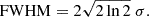
Given that the spectra of SNe II and IIb appear similar at early phases due to the presence of H and He I λ5876, we investigate whether they exhibit distinguishable properties. To do so, we examine how prototypical objects of each SN type evolve over time. Figure 4 shows the spectral evolution from the explosion to 30 days post-explosion for the type II SNe 1999em and 2013ej and the type IIb SNe 1993J and 2011dh.
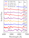 |
Fig. 4. Evolution of type II SNe 1999em (Leonard et al. 2001) (red) and 2013ej (Valenti et al. 2013) (orange) and type IIb SNe 1993J (Barbon et al. 1995) (blue) and 2011dh (Valenti et al. 2013; Ergon et al. 2014) (purple). The epoch of each of the spectra is computed from the explosion date. The dotted vertical line marks the rest-wavelength corresponding to Hβ; the dashed line is the He I λ5876 feature, and the continued line is Hα. |
By examining the spectral evolution in each SN, we identified specific features that exhibit distinct tendencies based on their classification. In the first days after the explosion, both SNe II and IIb often display a featureless blue continuum (Matheson et al. 2000a; Arcavi 2017; Hillier & Dessart 2019), which is the result of the high temperatures of the ejected material during that phase. As the ejecta cools down, broader lines, such as the hydrogen Balmer series and He I λ5876, emerge. Given that the H and He I lines are present in both SN types, we considered them as primary indicators. However, despite the fact that this property is shared among these two classes, notable differences in the evolution and shape of Hα and He I λ5876 are apparent (Figure 4). In the first one to two weeks, both types exhibit strong H lines, but their evolutionary patterns begin to diverge. For instance, for SNe II, Hα develops a well-defined P-Cygni profile. In contrast, in SNe IIb, Hα transitions towards a flat-topped profile, which eventually begins to split into two components due to the emergence of He I λ6678 (Holmbo et al. 2023). The presence and strength of this He I line can vary significantly between individual SNe, which can complicate the analysis of the Hα emission profile.
Subtle differences in the spectra of SNe II and IIb are also visible in the Hα absorption and He I line λ5876. The Hα absorption profile is typically much broader throughout the evolution of SNe IIb compared to SNe II. Additionally, the He I line λ5876 emerges earlier and is generally stronger in SNe IIb. This behaviour is likely a result of the partial stripping of the H envelope in SNe IIb.
We also examined the Hβ (λ4861) line, which shows differences between SNe II and IIb, similarly to Hα. However, given that Hβ is affected by the Iron lines around it, we excluded it from our analysis due to the complexities in its characterisation. The feature is marked with a dotted vertical line in Figure 4. In consequence, our analysis is focused only on the Hα absorption feature and the He I λ5876 line.
3.3. Median spectra
To visualise the main spectroscopic differences between SNe II, IIb and 87A-like, we compute the median spectrum of each type by including all the spectra in our final sample, following a similar procedure as Liu et al. (2016). This includes 188 SNe II, 199 SNe IIb and 6 SNe 87A-like between 0-40 days after explosion. Due to the limited number of SN 87A-like objects, the median spectrum for this group may not fully represent its characteristics. Nevertheless, we decided to include it because some SNe 87A-like are often mis-classified (see Section 4.1). The resulting median spectra for the three SN types are plotted in Figure A.2. The spectra were normalised by scaling them to the median value of a common reference wavelength range, ensuring their fluxes match at a specific wavelength. This process allows a direct comparison of spectral features across different objects while preserving their relative shapes. The resolution of the available data constrains the quality of the median spectra. While spectra with very poor resolution were excluded from our sample, some noisy spectra worsened the quality of the median spectrum, which is evident in Figure A.2.
A comparison between the three median spectra reveals common features with notable differences in the strength and width of the line depending on their type. In SNe IIb, both Hα and He I λ5876 are broader than in SNe II and 87A-like. In contrast, the spectrum of SNe II appears to be still dominated by the continuum, with Hα and He I λ5876 barely seen. For SNe 87A-like, spectral differences are also observed, although they are classified based on their photometry. The SN 87A-like median spectrum displays a well-defined Hα P-Cygni profile with a broad emission line. The He I λ5876 is also prominent. These findings align with our visual inspection.
Given that the spectral features change based on the SN phase, we perform a more detailed analysis of the median spectra over time. We computed it for SNe II and IIb within the four-time intervals: 0–10 days post-explosion, 10–20 days, 20–30 days, and 30–40 days. The resulting median spectra are presented in Figure 5, where SNe IIb are represented in blue and SNe II in red. Due to the limited data for SNe 87A-like, we could not compute their median spectra for specific time intervals.
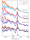 |
Fig. 5. Comparison between the median spectra of SNe II and IIb in different time ranges: 0–10 days post-explosion, 10–20 days, 20–30 days and 30–40 days. Blue spectra correspond to SNe IIb, and red spectra to SNe II. The dashed vertical line marks the rest wavelength of He I (λ5876), while the continuous line marks the rest wavelength of Hα. The shaded regions represent the Median Absolute Deviation (MAD), which represents dispersion around the median. |
The median spectra constructed within time intervals show more explicit evolutionary tendencies for each SN type. Notably, the Hα line dominates the spectrum of both classes. In the early phases, the absorption of the H lines (Hα and Hβ) is stronger in SNe IIb and remains so throughout their evolution up to 40 days. Furthermore, the He I line emerges within the first 10 days in SNe IIb, whereas in SN II, it appears at ∼10 days post-explosion. In SNe II, both Hα and He I also increase their strength over time, which can complicate classification depending on the specific characteristics of each SN. However, a key distinction lies in the shape of the lines, particularly Hα. In SNe II, the emission component remains strong at all phases, and the P-Cygni profile is well-defined.
Furthermore, a comparison between the median spectra of our SNe IIb sample and those presented by Liu et al. (2016) reveals strong similarities. In both cases, the Hα line shows broad absorption with a flattened-topped emission component, accompanied by a strengthening He I line that becomes more prominent as the SN evolves. Although Liu et al. (2016) sample does not cover phases as early as those analysed in this work, the median spectra between 10 and 40 days post-explosion are consistent across both works.
Examining the early spectra of SNe II, IIb, and 87A-like reveals significant observational differences in the strength and shape of the H and He lines among the different classes. These subtle differences enable early characterisation and more reliable classifications. Therefore, the following analysis is focused on the Hα absorption feature and the He I λ5876 lines.
4. Results
4.1. Spectral measurements
In this section, we present the results of our measurements. The values for the pEW and FWHM covering the first 40 days after the explosion are presented in Figure 6. The colour bars on the right side indicate the SN phase. The analysis across the full-time interval (0–40 days) does not reveal a distinct separation into two clusters; instead, it shows a continuum where SNe IIb tend to dominate at higher values.
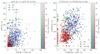 |
Fig. 6. Left panel: pEW of the Hα absorption profile versus the pEW of the He I λ5876 line measured across the full-time interval (0–40 days). The markers are established by SN type: SNe IIb are shown as blue triangles, SNe II as red circles, and SNe 87A-like as green squares. The colour bars on the right side indicate the SN phase. Right panel: Same as the left panel, but for the FWHM measurements. |
We examined the spectral features across smaller time intervals to investigate whether the observed continuum is intrinsic or a consequence of the broad time range considered (0–40 days). The results for the earliest two intervals (0–10 and 10–20 days) are presented in Figure 7. Within these intervals, the pEW and FWHM parameters reveal clear trends: SNe IIb consistently exhibit stronger Hα and He I features throughout the entire early time range. Notably, an intermediate region is observed around 25 Å in the pEW of both Hα and He I, as well as around 125 Å for Hα and 200 Å for He I in the FWHM. This overlap between the two populations further supports the continuum observed in the full-time interval (0–40 days). However, we note that the overlap between the groups becomes more significant as time passes. Specifically, the later the analysed time range, the greater the overlap, as the SN II values grow stronger as time passes (see Figures A.3 and A.4 in the Appendix A). This highlights the important role that the epoch of the SN will have in our analysis and the development of our method. A summary of the pEW and FWHM values for each SN type at each time interval is presented in Appendix B (see Table B.4).
 |
Fig. 7. pEW and FWHM values of Hα line and He I λ5876 for 0–10 days and 10–20 days. The markers are established by SN type: SNe IIb are shown as blue triangles, SNe II as red circles, and SNe 87A-like as green squares. The colour bars on the right side indicate the SN phase. The pEW measurements are in the top panels, and the FWHM measurements are in the bottom panels. In the left panels, we show the measurements within 0–10 days and in the right panels, between 10–20 days. |
We also find that although SNe 87A-like objects are spectroscopically similar at all phases to SNe II, they exhibit notably higher values, especially in the Hα absorption feature (Figures 6 and 7). Despite this, we excluded them from further analyses due to their low numbers.
To evaluate the statistical significance of our results, we applied the Kolmogorov-Smirnov test (KS test). This non-parametric method computes the maximum difference between the cumulative distribution function (CDF) of two data sets under the null hypothesis that both groups were drawn from populations with identical distributions. The KS test results for the comparison of the pEW and FWHM of Hα and He I between SNe II and IIb are summarised in Table 2. The table includes the KS statistic (greatest difference between the two CDFs) and the corresponding p-value (significance of the difference obtained) for each time interval. A p-value < 0.05 indicates the rejection of the null hypothesis, suggesting a statistically significant difference between the two groups.
KS-statistic run for our measurements. Separately for the pEW and FWHM results for the lines of Hα and He I.
From Table 2, we observe that most distributions have p-values significantly below the 0.05 threshold, indicating a meaningful separation between the SN II and IIb. The two samples exhibit statistically significant differences in the earliest 30 days post-explosion, with the most clear separation occurring within a 10 to 20-day interval. These findings support our hypothesis that SNe II and IIb display differences in their early spectral evolution, reinforcing the possibility of identifying them based on pEW and FWHM values.
The obtained KS test values suggest that while early-time observations can effectively differentiate between the two types based on pEW values, this distinction becomes less clear as SNe evolve. Interestingly, the greatest difference between SN II and IIb is observed during the 10 to 20-day interval rather than the earlier range (0–10 days). This is likely because both types are characterised by a blue featureless spectrum without prominent features soon after the explosion. Even as H lines emerge, they may still be weak, lacking sufficient signatures to differentiate between SNe II and IIb. Consistent with this, we find no significant difference in the Hα FWHM distribution during the first 10 days post-explosion.
From 30 days post-explosion, classifying SNe II and IIb based on the analysed spectral features becomes increasingly challenging due to the significant overlap between the two populations. For the 30–40-day interval, the p-values exceed the significance threshold across all analysed distributions, indicating that the differences between the pEW and FWHM of the two SN types decrease as their spectra evolve. Although the reduced number of spectra may influence the results, the physical convergence of spectral features also contributes. Around 30 days after explosion, the Hα line in SNe II typically strengthens, reaching intensities comparable to those observed in SNe IIb. At the same time, the He I line is often blended with the emerging Na I feature, particularly for SNe II (Gutiérrez et al. 2017). Nevertheless, the distinction between the two types remains clear at this stage when considering additional spectral features beyond Hα and He I. Indeed, by ∼30 days post-explosion, the Hα P-Cygni profile in SNe IIb begins to exhibit distinct characteristics of this subtype. Notably, the He I λ6678 feature, located near the peak of Hα, becomes more prominent, indicating an interference in the emission of the H feature. Additionally, He I lines emerge at this phase, providing robust criteria for distinguishing between SNe II and IIb.
4.2. Machine learning methods
Machine learning methods offer powerful tools for identifying and analysing differences between the studied classes. These techniques are particularly useful for uncovering patterns and relationships that may remain hidden by traditional approaches. By handling complex, non-linear patterns, machine learning methods can effectively identify the features that distinguish the classes. This subsection explores our previous results by employing various machine-learning techniques. These include density contours, quadratic discriminant analysis (QDA), T-distributed stochastic neighbour embedding (t-SNE), linear discriminant analysis (LDA), and random forest classifier(RFC).
4.2.1. Density contours
To further investigate the effect of overlapping values and the potential separation between the two SN types, we analysed their density evolution using a kernel density estimate (KDE). This method, which applies a Gaussian kernel with bandwidth = 1.0 by default, smooths the observations and produces a continuous estimate of the bivariate probability density. As a result, KDE offers a clearer representation of the data through continuous probability density curves.
Figure 8 illustrates the density contours of the pEW measurements. The comparison between the pEW of the Hα and He I demonstrates that SN II measurements are intensely concentrated within a narrow region below (20, 20) Å throughout the 0–40-day period. However, a noticeable increase in the density contours for SNe II appears after approximately 20 days, with the contours continuing to expand over time. Along the y-axis, a significant strengthening of the Hα absorption is observed, reaching values of approximately 80 Å by 20 days post-explosion. In contrast, the He I feature gradually increases, extending its outer density contours to around 40 Å.
 |
Fig. 8. Density contours of SNe II (in red) and IIb (in blue) based on the pEW measurements. The colour bars on the right side indicate the normalised density values, with darker colours representing higher densities. Each plot represents the density contours at different time intervals, as indicated at the top of the figure. |
In comparison, the SN IIb population exhibit a broader range of values and less concentration compared to SNe II. Although some overlap exists between SNe IIb and II, their density contours separate with distinct central values. For SNe IIb, the central values shift over time, increasing from approximately (30, 30) Å in the early phases to around (70, 70) Å at later epochs. Notably, during the later epochs, the values for SNe IIb start to disperse, mimicking the behaviour observed in SNe II. This dispersion is particularly evident in the 30–40-day interval, where a secondary high-density contour emerges closer to the SN II contour centre, resulting in a broader overlap between the two populations. The increasing pEW values for both SN types contribute to this overlap, as highlighted in the comparison plots presented in the previous section.
A similar density contour analysis was also performed for the FWHM measurements (Figure A.5 in Appendix A). The results also indicate a separation between the two SN populations. However, the overlap between the datasets is significantly more pronounced and the concentration of points within specific regions for each population is less distinct.
4.2.2. Quadratic discriminant analysis
Considering the significance of the separation between the two SN types confirmed by the KS test for both pEW and FWHM across time intervals, we defined the separation boundaries using a machine-learning approach. Specifically, we applied the quadratic discriminant analysis (QDA) to establish the optimal decision boundary for classifying our data points. QDA uses quadratic decision surfaces to discriminate between the measurements of the two samples. It can be considered a generalisation of the linear discriminant analysis (LDA), as it is not limited to dividing the data by a straight line.
Defining these regions not only demonstrates that the two populations are separable but also visually captures the distinct evolution of the pEW and FWHM. In Figure 9, we present the separation defined by the QDA classifier for our sample, using the pEW measurements of He I λ5876 and Hα. The decision boundaries are shown for the full dataset over the first 40 days post-explosion and for the 0–10 and 10–20-day intervals. Notably, the overlap between the two SN types is significantly reduced in the earliest intervals compared to the full 40-day range, as the 90% probability region is more compact. A similar analysis was performed for other time intervals and for the FWHM measurements (details in Appendix A, Figures A.8 and A.10). However, as demonstrated by the density contours and the KS test results (Table 2), the separation based on FWHM values is less distinct than that based on the pEWs.
 |
Fig. 9. Decision boundaries defined by the QDA classifier based on the pEW measurements for SN II and IIb pEW are shown across three time intervals: 0–10 days (left), 10–20 days (middle) and 0–40 days after the explosion (right). The red region corresponds to predictions for SNe II, while the blue region represents SNe IIb. The decision regions with a filled contour indicate where the model assigns a given SN type. Black contour lines represent classification probability thresholds, with a solid line marking a 50% probability, dashed lines for 75%, and a dotted line for 90% of belonging to a specific class. |
4.2.3. tSNE + LDA
As an alternative method to demonstrate and visualise the behaviour of the two SN populations, we applied the t-SNE (Van der Maaten & Hinton 2008). This statistical technique is designed for visualising high-dimensional data by reducing it to lower-dimensional spaces, offering intuitive insights into how data is structured in higher dimensions. Unlike linear methods, t-SNE can separate data that cannot be divided by a straight line, overcoming the limitations posed by the shape of our measurements. This approach is particularly useful for uncovering underlying patterns and relationships within the data.
We used t-SNE to visualise our data, incorporating all the measured values for each SNe. This process reduced our 5D dataset (including the pEW and FWHM of Hα and He I, along with the SNe epoch) into a 2D representation. The two resulting t-SNE components represent the reduced dimensions, capturing the spatial arrangement of the data points while preserving the relationships from the high-dimensional space. Additionally, to further analyse the 2D t-SNE distribution, we classified the data using LDA.
The resulting 2D distribution for the 0–40-day interval is presented in Figure 10. The plot reveals a separation between SNe II and IIb, with each type exhibiting a higher distribution in distinct regions of the plot. This finding supports the hypothesis that the two SN types can be distinguished based on the observed features (pEW, FWHM, and epoch). However, a complete separation is not evident. This continuity aligns with the trends observed in the individual pEW and FWHM comparisons of Hα and He I. Visualising the data with the t-SNE method, as opposed to the QDA analysis, highlights a noticeable density decrease between the two populations, delineating two primary clusters, even though a mixed region remains visible. This 2D visualisation highlights, as discussed in Section 4, the behaviour of the 87A-like SNe, which appear in the region predominantly occupied by SNe IIb. This may be a consequence of the strong Hα line exhibited by the 87A-like events (see Figure 6). Results for the 2D distributions in other time intervals are shown in Appendix A (Figure A.12).
 |
Fig. 10. Resulting t-SNE 2D reduced plot, using a perplexity value of 20. The red and blue dots represent SNe II and IIb, respectively, while green triangles indicate 87A-like events. The figure is separated into two regions defined by the LDA, with the solid line representing the decision boundary found for the t-SNE projection. |
4.2.4. Random forest classifier
Finally, we employed a RFC to analyse the differences in the behaviour of the two SN types. This machine learning approach utilises multiple decision trees to classify SNe based on their specific characteristics. To prepare the data for the RFC, we constructed a feature matrix combining the spectral parameters (FWHM and pEW for both Hα and He I) with the SN phase. The dataset was split into training and testing sets using a 60/40 ratio, ensuring a robust training sample while maintaining a significant portion for testing predictive accuracy. The classifier was trained on the training sample and evaluated on the test sample, predicting the SN types based on the input parameters. Importantly, we introduced only one value per parameter for each SN to ensure accurate outputs.
To evaluate the RFC’s effectiveness in distinguishing between the two SN types, we applied two different sampling strategies. In the first approach, for SNe with multiple spectra, we randomly selected a single spectrum per object for inclusion in the analysis. In the second approach, we computed the average of all available spectra for each SN, including the phase, and used these averaged measurements as input to the RFC. Figure 11 presents the predicted probabilities for test sample SNe classified as type II under both strategies. As shown in Table 3, the classifier performed slightly better with the random selection method.
 |
Fig. 11. Probabilities assigned by the RFC based on five parameters (pEW and FWHM of Hα and He I, along with the epoch) within the first 40 days post-explosion. Top: Classification probabilities obtained by randomly selecting one spectrum per SN from those with multiple observations. Bottom: Probabilities computed using the average spectrum for each SN, combining all available spectra. |
Comparison of precision and recall scores for the different classification methods.
Based on the RFC probabilities, SNe classified as type II (in red) consistently received a high probability of obtaining the same classification by the RFC. Conversely, SNe IIb (in blue) were assigned a low probability of being classified as type II. These results confirm that the measured features used in our analysis effectively distinguish the two SN types. We also tested alternative data combinations introduced in the RFC, which resulted in less effective classifications; For comparison, these results are presented in Appendix A (see Figures A.13 and A.14).
The RFC provides a statistical method for identifying differences between these two SN types and is a practical tool for classifying or reclassifying new SNe. By adjusting the training sample percentage from 60% to the entire dataset and using the values of interest for a specific SN as the test sample, it is possible to estimate the likelihood of that SN belonging to each type. For this purpose, and given the demonstrated utility of the method, we selected the RFC model based on averaged spectral values as our preferred classification tool. This approach ensures consistent, non-variable input for each SN by integrating all available spectral data from the main sample.
5. Discussion
5.1. A continuum in the Hα pEW and FWHM
The diversity observed in CCSNe arises from the varying amounts of outermost layers retained by their progenitor stars before the explosion. SNe IIb exhibit a transitional behaviour, evolving from hydrogen-dominated to helium-dominated spectra, suggesting that their progenitors retained less hydrogen before explosion than those of SNe II.
Our results show a complex picture: (i) while the pEW and FWHM of Hα and He I are generally higher in SNe IIb than in SNe II, (ii) no definite separation exists between these parameters, indicating a continuum. The first finding is somewhat counterintuitive, as one might expect SNe II, which retain a more significant amount of H, to exhibit stronger spectral features. However, this can be explained by the differences in progenitor structure. In progenitor stars with a substantial hydrogen envelope, a greater fraction of the shock-deposited energy is radiated away, leading to lower kinetic energy per unit mass (Ekin/Mej) and, consequently, slower expansion velocities and narrower spectral lines. In contrast, SNe IIb, with their low-mass hydrogen envelopes, experience faster ejecta expansion, resulting in broader spectral lines (Dessart et al. 2024).
As for the second finding, theoretical models with varying orbital separations predict a continuum of light-curve morphologies for type Ib, IIb, and II SNe, reflecting a range of H-rich envelope masses (Dessart et al. 2024). However, the distinct differences in the LCs of SNe II and IIb suggest their progenitors have different properties (e.g. Arcavi et al. 2012; Pessi et al. 2019), challenging the idea of a continuous distribution in spectral parameters. Our results indicate that, while hydrogen retention plays a key role in shaping the observed properties of SNe II and IIb, other factors likely contribute to their observed diversity. Even if hydrogen retention follows a continuum, this does not necessarily imply that their progenitors belong to a single, continuous evolutionary sequence. Instead, they likely represent distinct endpoints influenced by multiple parameters.
5.2. Effectiveness of our method
After applying several statistical techniques to quantitatively analyse the behaviour and differences between Hα and He I in SNe II and IIb, we evaluated the potential utility and reliability of these findings as a foundation for a novel classification method.
Having already included all available higher-resolution spectra in our primary sample, we tested our results using SNe with lower-resolution spectra. To this end, we gathered all available SEDM spectra for SNe II and IIb from the Transient Name Server (TNS8), comprising 609 SNe II and 25 SNe IIb. Objects without accompanying light curve information were excluded, as the explosion date was necessary to constrain the SN phase. Thus, the final sample consisted of 106 SNe, as detailed in Table B.1 (Appendix B). We note the significant disparity in the number of SEDM spectra classified as SNe II versus SNe IIb: among the 106 SNe, 92 were classified as SNe II and 14 as SNe IIb. Additionally, we incorporated newly classified SNe that were released after compiling our main sample. This includes 36 newly classified objects (28 SNe II and 8 SNe IIb) along with two SNe (SN 2013gg and SN 2015dj) that were classified as SNe II on TNS but as SNe IIb on WISeREP and SN 2019oxi, which is a type II but was showing broad features. As a result, the comparison sample comprised 123 SNe II and 22 SNe IIb.
Following the same procedure as before, we measured the pEW and FWHM of Hα and He I λ5876 for the newly collected spectra. The results were then plotted within the density contours (Figure 12) and the QDA decision regions (Figure A.9, in Appendix A). Each SN was represented according to its official classification type as recorded in TNS. This approach enabled us to validate our method by re-evaluating the classification of spectra that exhibited potential signs of mis-classification.
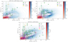 |
Fig. 12. pEW measurements of Hα and He I for the comparison sample (SEDM plus newly classified SNe) overlaid on the density contours of SNe II (red) and IIb (blue) obtained in Section 4.2.1 (same as Figure 9), for three time intervals: 0–10 days (left), 10–20 days (middle) and 0–40 days (right). The comparison sample is represented by SNe II as filled purple dots and SNe IIb as filled green triangles. Dark green circles correspond to SNe initially classified as type II but exhibiting SNe IIb-like properties. Open purple triangles represent SNe, which were initially classified as type IIb but spectroscopically belong to the SN II class. Pink squares denote SNe II showing 87A-like characteristics. Yellow stars highlight SNe II that appear to exhibit SNe IIb characteristics but lack sufficient data to confirm this classification. |
As shown in Figure 12, most of the objects from the comparison sample were correctly classified; however, a few SNe exhibit spectroscopic properties that more closely align with the opposite class. For instance, some SNe initially classified as type II display characteristics of SNe IIb (i.e. higher pEW values), and vice versa. In these cases, we cross-verified the classification by examining their LC shapes and rise times. Specifically, this decision is based on the observation that SNe II typically have shorter rise times than SNe IIb (Pessi et al. 2019) and that most of the SNe II exhibit a quasi-constant luminosity (a plateau) lasting several months. However, when the LC did not provide definitive confirmation, we conducted a more detailed spectral matching to refine the classification.
Through this re-evaluation process, we proved a potential mis-classification of 34 SNe. Among these, 26 objects initially classified as type II were found to align more closely with the properties of SNe IIb, while one SN, originally classified as SNe IIb, was determined to be better matched with SNe II. Notably, six SNe with insufficient photometric data (SN 2013gg, SNe 2018hqt, 2019noj, 2019oxi, 2024cgi and 2024lsi) show characteristics of both classes, providing inconclusive classifications. Lastly, SN 2020rmk was reclassified as a 87A-like event based on its spectral properties and exceptionally long-rise time (> 50 days). The re-classified objects are shown in Figure 12 and summarised in Tables B.2 and B.3 in the Appendix B.
To achieve a more accurate classification for those objects without a conclusive designation, we developed a Monte Carlo simulation with 500 iterations to compute their uncertainty. In each iteration, we resampled the base training set using bootstrapping, where some objects may be repeated and othersomitted, and retrained the RFC model. This process yielded a distribution of classification probabilities for each object, enabling a more informed assessment of SN type in cases where photometric classification is not feasible. As a result, we classified SNe 2024lsi and 2018hqt as type II and SNe 2024cgi and 2019noj as type IIb. For SN 2019oxi and SN 2013gg, the RFC assigned 83% probability of being a SN II and 17% of being a SN IIb, along with 55.6% and 44.4%, respectively, for the latter.
To evaluate how well each model balances the trade-off between identifying SNe of each type, we computed the precision and recall scores for each classification method. These metrics provide an overview of each method’s ability to classify the sample accurately. The precision measures the classifier’s ability to identify positive samples while minimising false positives correctly. This measures the proportion of correctly classified SNe among all predicted SNe, ensuring reliability. The recall reflects the classifier’s ability to identify all actual positive samples, minimising false negatives. It quantifies the proportion of actual SNe that were correctly identified by the model, ensuring completeness. Then, a high precision score indicates fewer false positives, while a high recall score means fewer wrong classifications. The equations for each of these metrics are as follows:
 (3)
(3)
 (4)
(4)
where TP are the true positives, cases where the model correctly classifies a SN, FP are false positives, where the given classification is incorrect, and FN are false negatives, cases where the model fails to identify the SN type. The metric scores for the methods are presented in Table 3. They all have similar precision and recall scores above 0.8 for both types.
5.3. Relative SN fractions
Once all SNe in our test sample were assigned a SN type following the methodology previously described, we compared these results with their initial classifications. We specifically analysed the impact of re-examined SEDM spectra on the original SN-type fractions. This comparison, presented in Figure 13, reveals a noticeable increase in the fraction of SNe IIb, with a 3.26%±0.13% rise (almost twice the initial fraction) in SEDM spectra classified as SNe IIb.
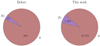 |
Fig. 13. Comparison of the fraction of SEDM spectra of each SN type before and after the performance of our re-classifications. |
The rates of CCSNe using the Lick Observatory Supernova Search volume-limited sample have been estimated in several works (e.g. Leaman et al. 2011; Li et al. 2011a,b; Maoz et al. 2011) and recently revised by Shivvers et al. (2017). They found that SNe II constitute approximately 70% of all CCSNe, while SESNe account for about 30%. Within SESNe, there are SNe Ib, Ic, and IIb. Based on known classifications and reclassifications, they estimated the true CCSNe fractions to be 69.6% for SNe II, 10.94% for SNe IIb, and 19.46% for other SESNe. More recently, Perley et al. (2020), using the ZTF Bright Transient Survey (BTS) magnitude-limited sample, found that hydrogen-rich SNe (SNe II, IIb, IIn, and superluminous SNe II) constitute 72.2% of all CCSNe. Within the hydrogen-rich SN class, SNe II are 69.05% of all the CCSNe, while the fraction corresponding to IIb is 5.10%. The remaining 25.85% is formed by SNe Ib, Ic, Ic-BL, and Ibn SESNe. These percentages correspond to the fractions excluding the SLSNe that were included in the analysis of Perley et al. (2020).
Based on the subtype ratio presented in Shivvers et al. (2017), we performed a similar analysis, including the same SN types, using publicly available TNS data collected from 2016 to 2024. Our results, presented in Figure 14, reveal discrepancies compared to Shivvers et al. (2017). The fraction of SNe II differs by 3.5%, while the SNe IIb fraction shows a disagreement of 5.6%. Compared to Perley et al. (2020), the SNe IIb fraction is almost the same, but their SNe II fraction is 4% smaller (this percentage is added to the SESN). While we recognise that this comparison is neither direct nor entirely equitable, since different selection effects than ours influence the referenced samples, we include it to provide a general perspective on how the relative fractions of SNe II and IIb vary when comparing our results with those of other studies.
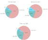 |
Fig. 14. CC-SNe fractions computed by Shivvers et al. (2017) (right-top), Perley et al. (2020) (bottom) and the fractions computed in this work by using the available data on TNS since 2016 (left-top). |
Considering our findings, even just the reanalysis of SEDM spectra resulted in a measurable shift in the SNe IIb fraction. This suggests that classification uncertainties, especially in distinguishing SNe II and IIb at early times, could significantly impact the CCSNe fraction estimates. If SNe IIb are not followed long enough, they may be mis-classified as SNe II. This effect could partly explain the observed difference in the SN IIb fractions between our TNS analysis and previous works.
5.4. Transitional events
During our analysis, we identified several peculiar objects, which are discussed in this section. SNe showing ambiguous behaviour in their spectra or LCs are considered “transitional objects”. These cases present conflicting classification indicators, as their photometry and spectroscopic characteristics suggest different SN types. The type II SNe 2019nyn, 2019uqp, 2019yyf, 2021agle, 2023rhj and 2024dgy were included in this discussion after their luminosity decay over 30 days post-peak was measured, revealing a magnitude difference comparable to that of the SNe IIb. Similarly, SN 2018arx (classified as a SN IIb) exhibited a LC shape similar to that of SNe II. For each transitional event, we also computed the RFC probability of belonging to each classification category (II/IIb/87A-like).
5.4.1. SNe II with type IIb-like luminosity declines
The SNe presented in Table 4 were classified as type II based on their spectral features; however, their luminosity decline within 30 days after peak is more consistent with SNe IIb. This discrepancy raises questions about their classification, suggesting possible transitional properties between the two types.
RFC probabilities for the ‘transitional objects’ identified through luminosity decline measurements.
The similar post-peak decline rates observed could be indicative of fast-declining SNe II (SNe IIL) or SNe IIb, both of which exhibit comparable light-curve behaviour during this phase. However, their early-time evolution diverges, with SNe IIb typically showing a slower rise to maximum light (Pessi et al. 2019). Some studies have suggested a degree of overlap between SNe IIL and IIb (e.g. Faran et al. 2014b; Reguitti et al. 2024), which can complicate photometric classification. Nevertheless, the spectroscopic features in our data strongly support a type II classification, making a IIb interpretation unlikely. Indeed, the probabilities assigned by the RFC strongly support their official classification as SNe II.
5.4.2. SNe II with mixed spectral and photometric properties
Some SNe display a combination of spectral and photometric characteristics that place them in the overlapping region between SNe II and IIb.
-
SN 2019oxi: Officially classified as a SN II, this object present notable deviations from the typical properties of SNe II. Its spectral features closely resemble those of SNe IIb, suggesting a possible reclassification. Although its photometric data benefits from a well-coverage follow-up, it does not provide a clear type identification, as it shows a slow rise over ∼40 days followed by a slow decline. By applying the RFC classification method combined with a Monte Carlo approach, we found that both techniques favour a type IIb classification. RFC probabilities: II: 0.60; IIb: 0.40; 87-like: 0.0.
-
SN 2018hoa: Officially classified as SNe II. The spectral line measurements are consistent with this classification, showing small values typical for SNe II. However, the LC exhibits a clear double peak morphology, a feature more commonly associated with SNe IIb. RFC probabilities: II: 0.50; IIb: 0.49; 87-like: 0.0.
-
SN 2024ehs: Officially classified as a SN II, it shows a bell-like shape LC, with a rising time of about 20 days and a rapid decline after the peak. The spectral measurements of H and He lines are not conclusive either, as they fall into the overlapping region. RFC probabilities at 2 days post-explosion: II:0.32; IIb:0.67; 87A-like:0.01; RFC probabilities at 16 days post-explosion: II:0.60; IIb:0.39; 87A-like:0.01.
5.4.3. SNe IIb showing type II-like photometric evolution
These SNe were classified as type IIb based on spectral features, yet their photometric behaviour resembles SNe II.
-
SN 2018arx: Although classified as a SN IIb and exhibiting a broad, flat-topped Hα, the He I line is very weak, causing it to fall into the overlapping region between the two populations. Regarding the photometry, it shows a peculiar, relatively constant luminosity that resembles a plateau. The RFC probabilities for this SN are: II: 0.36; IIb: 0.64; 87A-like: 0.00.
-
SN 2022emz: Spectroscopically, it exhibits the characteristics of a slowly evolving SN IIb, with a broad and deep He I line and a flat top Hα. However, upon analysing its LC, a constant luminosity is observed for nearly 100 days after the peak. This behaviour is usual of slow-declining SNe II (SNe IIP). On the other hand, the rise to the peak aligns with the average time exhibited by SNe IIb (Pessi et al. 2019). The RFC probabilities for this object are as follows: II:0.0; IIb:1.00; 87A-like:0.00.
5.5. A new tool to classify SNe II and IIb based on early spectra
We also defined two alternative classification methods that could indeed be used to complement the density contours and QDA regions. First, we performed again a RFC (see section 4.2.4), taking this time our entire sample as a training sample and a newly measured SN as a test sample. This way, we achieve the probabilities for that SN to belong to each type. The probabilities for the SEDM spectra and new classifications are presented in Tables B.3 and B.2. Second, we developed the possibility of plotting the newly measured SNe on our t-SNE plots. So far, we can see whether it falls in the cluster formed by a majority of type II or IIb SNe. This would allow us to have different approaches to interpreting the values obtained for the new SNe.
6. Conclusions
In this paper, we present a detailed analysis of the early spectra of SNe II and IIb to uncover their diversity. The 866 spectra of 393 SNe composing our main sample were analysed using the pEW and FWHM of the Hα and He I λ5876 features. Statistical methods and machine-learning techniques were applied to identify differences between SNe II and IIb. Our main results are listed below:
-
We find that pEW and FWHM of Hα and He I λ5876 in SNe IIb display larger values than those of SNe II over the entire evolution, with the most significant differences occurring in the early phases, particularly in the 10–20-day interval.
-
The population density evolution reveals a clear separation in the pEW of SNe II and IIb. In particular, SNe II consistently exhibit high-density concentrations around 20 Å, while SNe IIb reach 60–80 Å values. Despite this distinction, the two populations seem to form a continuum in spectral properties.
-
The QDA analysis shows that SNe II and IIb exhibit distinct pEW evolution patterns, with the greatest separation occurring within the first ten days. In contrast, differences based on FWHM measurements are less pronounced.
-
t-SNE+LDA effectively separated the two types, supporting their distinction based on observed features. However, the continuity between the two clusters persists. This suggests a gradual transition, rather than a strict boundary, between the populations.
-
The RFC confirms the distinct characteristics of the two groups and demonstrates the effectiveness of these parameters (pEW and FWHM of Hα and He I) as classification criteria. Additionally, it enables the classification of newly observed SNe.
-
We carried out a validation of the method using low-resolution SEDM spectra and newly classified SNe. We identified 34 possible mis-classified SNe within the re-analysed sample. Based on these revised classifications, we recalculated the SEDM fraction for each SNe type, leading to a notable increase in the percentage of SNe IIb reported in WISERep from 4.0% to 7.26% (see Figure 13), nearly doubling its original value.
We developed a new classification method for early SNe II and IIb based on quantified differences in spectral features during their early evolution. Using the obtained results, we computed classification probabilities with the RF classifier and plotted the measurements within defined regions, enabling a clear classification assessment. This approach not only improves our understanding of the early phases of SN evolution, but also serves as a valuable tool for enhancing classification accuracy in future observations. Our findings indicate that mis-classification significantly impacts the actual CCSNe rate. The reclassification of SEDM spectra has improved the accuracy of previously available classification data, highlighting the robustness of our method.
Data availability
All spectra used in our analysis are publicly available, with references listed in Table B.5. They can be downloaded from WISeREP or are published in the literature. The full version of Table B.5 is available at the CDS via https://cdsarc.cds.unistra.fr/viz-bin/cat/J/A+A/702/A128.
All classification tools developed in this study, along with the computed median spectra for each time interval, are publicly available at https://doi.org/10.5281/zenodo.15756198 (https://zenodo.org/communities/sndata/) to facilitate broader use.
Non-detections correspond to fluxes below the detection threshold. In these cases, ATLAS and ZTF report upper-limit magnitudes based on the image depth, typically 3σ for forced photometry in ATLAS, and 5σ in ZTF.
Following Blondin & Tonry (2007), we only considered matches with rlap ≥5 and lap ≥0.4.
The best-fitting SN template is identified via a χ2 minimisation procedure.
Acknowledgments
We thank the anonymous referee for the comments and suggestions that have helped us to improve the paper. We thank Maria Kopsacheili, Koraljka Muzic, Joseph Anderson, Luc Dessart and Bastián Ayala for valuable discussions. M.G.B.’s work has been carried out within the framework of the doctoral program in Physics of the Universitat Autònoma de Barcelona. The M.G.B., C.P.G., L.G. research group acknowledges financial support from the Spanish Ministerio de Ciencia e Innovación (MCIN) and the Agencia Estatal de Investigación (AEI) 10.13039/501100011033 under the PID2020-115253GA-I00 HOSTFLOWS and PID2023-151307NB-I00 SNNEXT project, from Centro Superior de Investigaciones Científicas (CSIC) under the projects PIE 20215AT016, ILINK23001, COOPB2304, and the program Unidad de Excelencia María de Maeztu CEX2020-001058-M, and from the Departament de Recerca i Universitats de la Generalitat de Catalunya through the 2021-SGR-01270 grant. C.P.G. acknowledges financial support from the Secretary of Universities and Research (Government of Catalonia) and by the Horizon 2020 Research and Innovation Programme of the European Union under the Marie Skłodowska-Curie and the Beatriu de Pinós 2021 BP 00168 programme.
References
- Anderson, J. P., González-Gaitán, S., Hamuy, M., et al. 2014, ApJ, 786, 67 [Google Scholar]
- Angus, C., Wiseman, P., Swann, E., et al. 2019, TNS Classification Report, 2019, 1 [Google Scholar]
- Arcavi, I. 2017, arXiv e-prints [arXiv:1710.03759] [Google Scholar]
- Arcavi, I., Gal-Yam, A., Cenko, S. B., et al. 2012, ApJ, 756, L30 [NASA ADS] [CrossRef] [Google Scholar]
- Arcavi, I., Burke, J., Hiramatsu, D., et al. 2019, TNS Classification Report [Google Scholar]
- Barbon, R., Ciatti, F., & Rosino, L. 1979, A&A, 72, 287 [Google Scholar]
- Barbon, R., Benetti, S., Cappellaro, E., et al. 1995, A&AS, 110, 513 [NASA ADS] [Google Scholar]
- Bellm, E. C., Kulkarni, S. R., Graham, M. J., et al. 2019, PASP, 131, 018002 [Google Scholar]
- Bersten, M. C., Benvenuto, O. G., Nomoto, K., et al. 2012, ApJ, 757, 31 [Google Scholar]
- Blagorodnova, N., Neill, J. D., Walters, R., et al. 2018, PASP, 130, 035003 [Google Scholar]
- Blondin, S., & Tonry, J. L. 2007, ApJ, 666, 1024 [NASA ADS] [CrossRef] [Google Scholar]
- Bose, S., Holmbo, S., Mattila, S., Classification, T. N. S., et al. 2019, Report. [Google Scholar]
- Burke, J., Hiramatsu, D., Howell, D. A., McCully, C., & Pellegrino, C. 2019, TNS Classification Report [Google Scholar]
- Burke, J., Hiramatsu, D., Howell, D. A., McCully, C., & Pellegrino, C. 2020, TNS Classification Report [Google Scholar]
- Cartier, R., & Ugarte, P. 2019, TNS Classification Report, 2019, 1 [Google Scholar]
- Childress, M. J., Tucker, B. E., Yuan, F., et al. 2016, PASA, 33, e055a [Google Scholar]
- Clocchiatti, A. 2002, IAU Circ., 7793, 2 [NASA ADS] [Google Scholar]
- de Jaeger, T., Zheng, W., Stahl, B. E., et al. 2019, MNRAS, 490, 2799 [NASA ADS] [CrossRef] [Google Scholar]
- della Valle, M., & Bianchini, A. 1992, IAU Circ., 5558, 3 [Google Scholar]
- Dessart, L., Gutiérrez, C. P., Ercolino, A., Jin, H., & Langer, N. 2024, A&A, 685, A169 [NASA ADS] [CrossRef] [EDP Sciences] [Google Scholar]
- Ergon, M., Sollerman, J., Fraser, M., et al. 2014, A&A, 562, A17 [NASA ADS] [CrossRef] [EDP Sciences] [Google Scholar]
- Evans, R., White, B., & Bembrick, C. 2001, IAU Circ., 7772, 1 [Google Scholar]
- Faran, T., Poznanski, D., Filippenko, A. V., et al. 2014a, MNRAS, 442, 844 [NASA ADS] [CrossRef] [Google Scholar]
- Faran, T., Poznanski, D., Filippenko, A. V., et al. 2014b, MNRAS, 445, 554 [NASA ADS] [CrossRef] [Google Scholar]
- Filippenko, A. V. 1988, AJ, 96, 1941 [CrossRef] [Google Scholar]
- Filippenko, A. V., Matheson, T., & Ho, L. C. 1993, ApJ, 415, L103 [NASA ADS] [CrossRef] [Google Scholar]
- Folatelli, G., Bersten, M. C., Benvenuto, O. G., et al. 2014, ApJ, 793, L22 [NASA ADS] [CrossRef] [Google Scholar]
- Galbany, L., Hamuy, M., Phillips, M. M., et al. 2016, AJ, 151, 33 [NASA ADS] [CrossRef] [Google Scholar]
- Gal-Yam, A. 2016, arXiv e-prints [arXiv:1611.09353] [Google Scholar]
- Gal-Yam, A., Bufano, F., Barlow, T., et al. 2008, ApJ, 685, L117 [NASA ADS] [CrossRef] [Google Scholar]
- Goldwasser, S., Yaron, O., Sass, A., et al. 2022, TNS AstroNote, 191, 1 [Google Scholar]
- González-Gaitán, S., Tominaga, N., Molina, J., et al. 2015, MNRAS, 451, 2212 [CrossRef] [Google Scholar]
- Graham, M. J., Kulkarni, S. R., Bellm, E. C., et al. 2019, PASP, 131, 078001 [Google Scholar]
- Gutiérrez, C. P., Anderson, J. P., Hamuy, M., et al. 2017, ApJ, 850, 89 [CrossRef] [Google Scholar]
- Hamuy, M., Pinto, P. A., Maza, J., et al. 2001, ApJ, 558, 615 [NASA ADS] [CrossRef] [Google Scholar]
- Hamuy, M., Deng, J., Mazzali, P. A., et al. 2009, ApJ, 703, 1612 [NASA ADS] [CrossRef] [Google Scholar]
- Hillier, D. J., & Dessart, L. 2019, A&A, 631, A8 [NASA ADS] [CrossRef] [EDP Sciences] [Google Scholar]
- Hiramatsu, D., Arcavi, I., Burke, J., et al. 2018, TNS Classification Report, 2018, 1 [Google Scholar]
- Hiramatsu, D., Howell, D. A., Moriya, T. J., et al. 2021, ApJ, 913, 55 [CrossRef] [Google Scholar]
- Holmbo, S., Stritzinger, M., Karamehmetoglu, E., et al. 2023, A&A, 675, A83 [NASA ADS] [CrossRef] [EDP Sciences] [Google Scholar]
- Hosseinzadeh, G., Arcavi, I., Valenti, S., Howell, D. A., & McCully, C. 2016, TNS Classification Report, 2016-213 [Google Scholar]
- Howell, D. A., Sullivan, M., Perrett, K., et al. 2005, ApJ, 634, 1190 [NASA ADS] [CrossRef] [Google Scholar]
- Janka, H.-T., Langanke, K., Marek, A., Martínez-Pinedo, G., & Müller, B. 2007, Phys. Rep., 442, 38 [NASA ADS] [CrossRef] [Google Scholar]
- Kunkel, W., Madore, B., Shelton, I., et al. 1987, IAU Circ., 4316, 1 [Google Scholar]
- Leaman, J., Li, W., Chornock, R., & Filippenko, A. V. 2011, MNRAS, 412, 1419 [NASA ADS] [CrossRef] [Google Scholar]
- Leonard, D. C., Filippenko, A. V., Gates, E. L., et al. 2001, PASP, 114, 35 [Google Scholar]
- Li, W., Chornock, R., Leaman, J., et al. 2011a, MNRAS, 412, 1473 [NASA ADS] [CrossRef] [Google Scholar]
- Li, W., Leaman, J., Chornock, R., et al. 2011b, MNRAS, 412, 1441 [NASA ADS] [CrossRef] [Google Scholar]
- Liu, Y.-Q., Modjaz, M., Bianco, F. B., & Graur, O. 2016, ApJ, 827, 90 [NASA ADS] [CrossRef] [Google Scholar]
- Maoz, D., Mannucci, F., Li, W., et al. 2011, MNRAS, 412, 1508 [Google Scholar]
- Matheson, T., Filippenko, A. V., Barth, A. J., et al. 2000a, AJ, 120, 1487 [NASA ADS] [CrossRef] [Google Scholar]
- Matheson, T., Filippenko, A. V., Ho, L. C., Barth, A. J., & Leonard, D. C. 2000b, AJ, 120, 1499 [NASA ADS] [CrossRef] [Google Scholar]
- Matheson, T., Filippenko, A. V., Li, W., Leonard, D. C., & Shields, J. C. 2001, AJ, 121, 1648 [NASA ADS] [CrossRef] [Google Scholar]
- Maund, J. R. 2019, ApJ, 883, 86 [Google Scholar]
- Maund, J. R., Smartt, S. J., Kudritzki, R. P., Podsiadlowski, P., & Gilmore, G. F. 2004, Nature, 427, 129 [NASA ADS] [CrossRef] [Google Scholar]
- Minkowski, R. 1979, A Source Book in A&A, 1900-1975 (Harvard University Press), 478 [Google Scholar]
- Modjaz, M., Blondin, S., Kirshner, R. P., et al. 2014, AJ, 147, 99 [Google Scholar]
- Morales-Garoffolo, A., Elias-Rosa, N., Bersten, M., et al. 2015, MNRAS, 454, 95 [CrossRef] [Google Scholar]
- Nakano, S., Aoki, M., Garnavich, P., Kirshner, R., & Berlind, P. 1996, IAU Circ., 6524, 1 [Google Scholar]
- Nakano, S., Aoki, M., Garnavich, P., Kirshner, R., & Stanek, K. 1997, IAU Circ., 6724, 1 [Google Scholar]
- Nakar, E., & Piro, A. L. 2014, ApJ, 788, 193 [NASA ADS] [CrossRef] [Google Scholar]
- Pastorello, A., Zampieri, L., Turatto, M., et al. 2004, MNRAS, 347, 74 [Google Scholar]
- Pastorello, A., Pumo, M., Navasardyan, H., et al. 2012, A&A, 537, A141 [NASA ADS] [CrossRef] [EDP Sciences] [Google Scholar]
- Perley, D. A., Fremling, C., Sollerman, J., et al. 2020, ApJ, 904, 35 [NASA ADS] [CrossRef] [Google Scholar]
- Pessi, P. J., Folatelli, G., Anderson, J. P., et al. 2019, MNRAS, 488, 4239 [NASA ADS] [CrossRef] [Google Scholar]
- Phillips, M., Suntzeff, N., Krisciunas, K., et al. 2001, IAU Circ., 7772, 2 [Google Scholar]
- Piranomonte, S., Carini, R., Benetti, S., & Yaron, O. 2019a, TNS Classification Report [Google Scholar]
- Piranomonte, S., Carini, R., Melandri, A., D’avanzo, P., & Yaron, O. 2019b, TNS Classification Report, 2019, 1 [Google Scholar]
- Pollas, C., & Pennypacker, C. 1987, IAU Circ., 4426, 1 [Google Scholar]
- Pun, C. S., Kirshner, R. P., Sonneborn, G., et al. 1995, ApJ, 99, 223 [Google Scholar]
- Rabinak, I., & Waxman, E. 2011, ApJ, 728, 63 [Google Scholar]
- Ragosta, F., Carini, R., Tartaglia, L., Benetti, S., & Yaron, O. 2021, TNS Classification Report [Google Scholar]
- Reguitti, A., Dastidar, R., Pignata, G., et al. 2024, A&A, 692, A26 [NASA ADS] [CrossRef] [EDP Sciences] [Google Scholar]
- Ripero, J., Garcia, F., Rodriguez, D., et al. 1993, IAU Circ., 5731, 1 [NASA ADS] [Google Scholar]
- Ruiz-Lapuente, P., Kidger, M., Lopez, R., & Canal, R. 1990, AJ, 100, 782 [Google Scholar]
- Ryder, S. D., Sadler, E., Subrahmanyan, R., et al. 2005, International Astronomical Union Colloquium (Cambridge University Press), 192, 123 [Google Scholar]
- Ryder, S. D., Van Dyk, S. D., Fox, O. D., et al. 2018, ApJ, 856, 83 [NASA ADS] [CrossRef] [Google Scholar]
- Sanders, E., Li, W., & Lotoss 2002, IAU Circ., 7944, 2 [Google Scholar]
- Sanders, N. E., Soderberg, A. M., Gezari, S., et al. 2015, ApJ, 799, 208 [NASA ADS] [CrossRef] [Google Scholar]
- Sapir, N., & Waxman, E. 2017, ApJ, 838, 130 [NASA ADS] [CrossRef] [Google Scholar]
- Schlegel, E. M. 1990, MNRAS, 244, 269 [NASA ADS] [Google Scholar]
- Schmidt, B. P., Kirshner, R. P., Schild, R., et al. 1993, AJ, 105, 2236 [NASA ADS] [CrossRef] [Google Scholar]
- Shigeyama, T., Suzuki, T., Kumagai, S., et al. 1994, ApJ, 420, 341 [NASA ADS] [CrossRef] [Google Scholar]
- Shingles, L., Smith, K. W., Young, D. R., et al. 2021, TNS AstroNote, 7, 1 [Google Scholar]
- Shivvers, I., Modjaz, M., Zheng, W., et al. 2017, PASP, 129, 054201 [NASA ADS] [CrossRef] [Google Scholar]
- Shivvers, I., Filippenko, A. V., Silverman, J. M., et al. 2019, MNRAS, 482, 1545 [Google Scholar]
- Silverman, J. M., Mazzali, P., Chornock, R., et al. 2009, PASP, 121, 689 [Google Scholar]
- Sit, T. 2022, TNS Classification Report [Google Scholar]
- Smartt, S. J., Maund, J. R., Hendry, M. A., et al. 2004, Science, 303, 499 [NASA ADS] [CrossRef] [Google Scholar]
- Smartt, S., Eldridge, J., Crockett, R., & Maund, J. 2009, MNRAS, 395, 1409 [CrossRef] [Google Scholar]
- Smartt, S. J., Valenti, S., Fraser, M., et al. 2015, A&A, 579, A40 [NASA ADS] [CrossRef] [EDP Sciences] [Google Scholar]
- Smith, K. W., Williams, R. D., Young, D. R., et al. 2019, Res. Notes AAS, 3, 26 [Google Scholar]
- Smith, K. W., aryd Smartt, S. J., Young, D. R., Tonry, J. L., et al. 2020, Publ. Astron. Soc. Pacific, 132, 085002 [Google Scholar]
- Spiro, S., Pastorello, A., Pumo, M., et al. 2014, MNRAS, 439, 2873 [Google Scholar]
- Srivastav, S., Smartt, S. J., McBrien, O., Classification, T. N. S., et al. 2021, Report. [Google Scholar]
- Taddia, F., Stritzinger, M. D., Sollerman, J., et al. 2012, A&A, 537, A140 [NASA ADS] [CrossRef] [EDP Sciences] [Google Scholar]
- Taddia, F., Sollerman, J., Fremling, C., et al. 2016, A&A, 588, A5 [NASA ADS] [CrossRef] [EDP Sciences] [Google Scholar]
- Tody, D. 1986, Instrumentation in astronomy VI, Vol. 627, (SPIE), 733 [Google Scholar]
- Tody, D. 1993, Astronomical Data Analysis Software and Systems II, 52, 173 [Google Scholar]
- Tonry, J. L., Denneau, L., Heinze, A. N., et al. 2018, PASP, 130, 064505 [Google Scholar]
- Valenti, S., Sand, D., Pastorello, A., et al. 2013, MNRAS, 438, L101 [Google Scholar]
- Van der Maaten, L., & Hinton, G. 2008, J. Mach. Learn. Res., 9 [Google Scholar]
- Van Dyk, S. D., Li, W., & Filippenko, A. V. 2003, PASP, 115, 1289 [NASA ADS] [CrossRef] [Google Scholar]
- Wiseman, P., Angus, C., Frohmaier, C., Swann, E., & Irani, I. 2019, TNS Classification Report, 2019, 1 [Google Scholar]
- Wood-Vasey, W., Aldering, G., Nugent, P., & Chassagne, R. 2003, IAU Circ., 8082, 1 [Google Scholar]
- Woosley, S., Eastman, R. G., Weaver, T. A., & Pinto, P. A. 1994, ApJ, 429, 300 [NASA ADS] [CrossRef] [Google Scholar]
- Yaron, O., & Gal-Yam, A. 2012, PASP, 124, 668 [Google Scholar]
- Zheng, W., & Filippenko, A. V. 2015, ATel, 7366, 1 [Google Scholar]
Appendix A: Figures
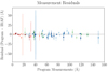 |
Fig. A.1. Residuals between the pEW and FWHM values measured with our interactive program and those obtained with IRAF are shown as (programme: IRAF) plotted against the programme-derived values. Data points are colour-coded by SN type: SNe II are shown in warm colours, while SNe IIb are in cool tones. Different colours represent different SNe. |
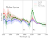 |
Fig. A.2. Comparison between the median spectrum for SNe II (red), SNe IIb (blue) and SN 87A-like (green) constructed from all spectra in our sample (from explosion to 40 days post-explosion). The shaded regions represent the Median Absolute Deviation (MAD), providing a measure of dispersion around the median. |
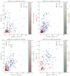 |
Fig. A.3. pEW values of the Hα vs the same measurements for He I λ5876 for separated time ranges since explosion: 0-10 days, 10-20 days, 20-30 days, and 30-40 days. The markers are established by SN type, corresponding to type SNe IIb: blue triangles; SNe II: red circles, and SNe 87A-like: green squares. The colour bars show how the colour intensity changes depending on the number of days since the explosion. |
 |
Fig. A.4. FWHM of the Hα (λ6563) line vs the same measurements for the He I (λ5876) line for separated time ranges since explosion: 0-10 days, 10-20 days, 20-30 days and 30-40 days. The markers are established by SN type, corresponding to type SNe IIb: blue triangles, SNe II: red circles, and SNe 87A-like: green squares. The colour bars show how the colour intensity changes depending on the number of days since the explosion. |
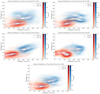 |
Fig. A.5. Density distribution of type II (in red) and IIb (in blue) population of our sample based on the FWHM measurements. We present the distribution for the different time ranges that we have analysed. |
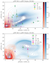 |
Fig. A.6. Density contours of the pEW along with the SEDM and the new classified SNe used as test sample for 20-30 and 30-40 days after explosion. The comparison sample is represented by SNe II as filled purple dots and SNe IIb as filled green triangles. Dark green circles correspond to SNe initially classified as type II but exhibiting SNe IIb-like properties. Open purple triangles represent SNe initially classified as type IIb but spectroscopically belonging to the SN II class. Pink squares denote type II SNe showing 87A-like characteristics. Yellow stars highlight type II SNe that appear to exhibit SNe IIb characteristics but lack sufficient data to confirm this classification. |
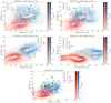 |
Fig. A.7. Density contours of the FWHM along with the SEDM and the new classified SNe used as test sample, are shown. The comparison sample is represented by SNe II as filled purple dots and SNe IIb as filled green triangles. Dark green circles correspond to SNe initially classified as type II but exhibiting SNe IIb-like properties. Open purple triangles represent SNe initially classified as type IIb but spectroscopically belonging to the SN II class. Pink squares denote type II SNe showing 87A-like characteristics. Yellow stars highlight type II SNe that appear to exhibit SNe IIb characteristics but lack sufficient data to confirm this classification. |
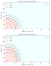 |
Fig. A.8. Decision boundaries defined by the QDA based on the measures performed for the II and IIb pEW for the following time ranges 20-30 days and 30-40 days after the explosion. The red region corresponds to the type II SNe, and the blue region to the IIb SNe. |
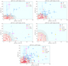 |
Fig. A.9. Ranges defined by QDA based on the measures performed for the II and IIb pEW along with the SEDM and the new classified SNe. The closed red dots mark the type II data points, the closed blue triangles the type IIb and the yellow square a 87A-like. The open markers are those that have been reclassified based on our method. So the open blue circles belong to the SNe that were first classified as type II and then reclassified as IIb. The open red triangles are those first classified as IIb and then reclassified as II in this work. The purple open stars are SNe classified as II that seem to exhibit characteristics of IIb but could not be confirmed. In Table B.2, we present the SNe included in the plots, together with their previous and updated classifications. |
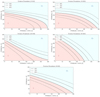 |
Fig. A.10. Decision boundaries defined by the QDA classifier based on the measures performed for the FWHM of SNe II and IIb at all the analysed time intervals. The red region corresponds to the SNe II, and the blue region to SNe IIb. |
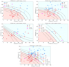 |
Fig. A.11. Ranges defined by QDA based on the measures performed for the II and IIb FWHM, along with the SEDM and the new classified SNe. The closed red dots mark the type II data points, the closed blue triangles the type IIb and the yellow square a 87A-like. The open markers are those that have been reclassified based on our method. So the open blue circles belong to the SNe that were first classified as type II and then reclassified as IIb. The open red triangles are those first classified as IIb and then reclassified as II in this work. The purple open stars are SNe classified as II that seem to exhibit characteristics of IIb but could not be confirmed. In Table B.2 we present the SNe included in the plots, together with their previous and updated classifications. |
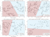 |
Fig. A.12. Projection of t-SNE with a perplexity value of 20, along with a LDA analysis of the obtained 2D plot for all the analysed time ranges. |
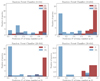 |
Fig. A.13. Probabilities given by the RFC for supernova spectra, with the data split into four time ranges after the explosion: 0–10 days, 10–20 days, 20–30 days, and 30–40 days. The classifier uses the pEW, FWHM, epoch, and type of each SN spectrum as input parameters, with 60% of the total sample used for training and the remaining 40% for testing. The red and blue bins correspond to SNe II and IIb, respectively. |
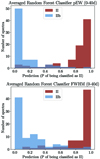 |
Fig. A.14. Left panel: Probabilities given by the RFC for the whole sample, taking into account the pEW measurements for all the spectra within the first 40 days after the explosion the SN, using %60 of the total sample as training sample and the rest as test sample. Right panel: Probabilities given by the RFC for the whole sample, taking into account only the FWHM measurements for all the spectra within the first 40 days after the explosion, using %60 of the total sample as training sample and the rest as test sample. The red and blue bins correspond to SNe II and IIb, respectively. |
Appendix B: Tables
SNe with lower resolution data
Reclassified SEDM spectra based on the regions we defined.
New SN classifications.
Evolution of the mean value of pEW and FWHM for each type over the examined time ranges along with their standard deviation.
Full SN sample.
All Tables
Reclassified SNe based on their spectral evolution and/or photometry properties.
KS-statistic run for our measurements. Separately for the pEW and FWHM results for the lines of Hα and He I.
Comparison of precision and recall scores for the different classification methods.
RFC probabilities for the ‘transitional objects’ identified through luminosity decline measurements.
Evolution of the mean value of pEW and FWHM for each type over the examined time ranges along with their standard deviation.
All Figures
|
Fig. 1. Histogram of the number of spectra per SN. In total, our sample is composed of 866 spectra for 393 SNe. |
| In the text | |
|
Fig. 2. Redshift distribution for the 393 SNe in our sample. The vertical lines indicated the median of the whole sample (solid black line) at 0.022, SNe II (dashed-dotted red line) at 0.021, and IIb (dashed blue line) at 0.023. |
| In the text | |
|
Fig. 3. Example of the pEW and FWHM measurement for the He I line. Top: Selection of the two regions to define the line to be measured. Bottom: Defined line and the Gaussian fitting for the pEW and FWHM computation. The different line colours represent the shifted measurements used to estimate the uncertainties. |
| In the text | |
|
Fig. 4. Evolution of type II SNe 1999em (Leonard et al. 2001) (red) and 2013ej (Valenti et al. 2013) (orange) and type IIb SNe 1993J (Barbon et al. 1995) (blue) and 2011dh (Valenti et al. 2013; Ergon et al. 2014) (purple). The epoch of each of the spectra is computed from the explosion date. The dotted vertical line marks the rest-wavelength corresponding to Hβ; the dashed line is the He I λ5876 feature, and the continued line is Hα. |
| In the text | |
|
Fig. 5. Comparison between the median spectra of SNe II and IIb in different time ranges: 0–10 days post-explosion, 10–20 days, 20–30 days and 30–40 days. Blue spectra correspond to SNe IIb, and red spectra to SNe II. The dashed vertical line marks the rest wavelength of He I (λ5876), while the continuous line marks the rest wavelength of Hα. The shaded regions represent the Median Absolute Deviation (MAD), which represents dispersion around the median. |
| In the text | |
|
Fig. 6. Left panel: pEW of the Hα absorption profile versus the pEW of the He I λ5876 line measured across the full-time interval (0–40 days). The markers are established by SN type: SNe IIb are shown as blue triangles, SNe II as red circles, and SNe 87A-like as green squares. The colour bars on the right side indicate the SN phase. Right panel: Same as the left panel, but for the FWHM measurements. |
| In the text | |
|
Fig. 7. pEW and FWHM values of Hα line and He I λ5876 for 0–10 days and 10–20 days. The markers are established by SN type: SNe IIb are shown as blue triangles, SNe II as red circles, and SNe 87A-like as green squares. The colour bars on the right side indicate the SN phase. The pEW measurements are in the top panels, and the FWHM measurements are in the bottom panels. In the left panels, we show the measurements within 0–10 days and in the right panels, between 10–20 days. |
| In the text | |
|
Fig. 8. Density contours of SNe II (in red) and IIb (in blue) based on the pEW measurements. The colour bars on the right side indicate the normalised density values, with darker colours representing higher densities. Each plot represents the density contours at different time intervals, as indicated at the top of the figure. |
| In the text | |
|
Fig. 9. Decision boundaries defined by the QDA classifier based on the pEW measurements for SN II and IIb pEW are shown across three time intervals: 0–10 days (left), 10–20 days (middle) and 0–40 days after the explosion (right). The red region corresponds to predictions for SNe II, while the blue region represents SNe IIb. The decision regions with a filled contour indicate where the model assigns a given SN type. Black contour lines represent classification probability thresholds, with a solid line marking a 50% probability, dashed lines for 75%, and a dotted line for 90% of belonging to a specific class. |
| In the text | |
|
Fig. 10. Resulting t-SNE 2D reduced plot, using a perplexity value of 20. The red and blue dots represent SNe II and IIb, respectively, while green triangles indicate 87A-like events. The figure is separated into two regions defined by the LDA, with the solid line representing the decision boundary found for the t-SNE projection. |
| In the text | |
|
Fig. 11. Probabilities assigned by the RFC based on five parameters (pEW and FWHM of Hα and He I, along with the epoch) within the first 40 days post-explosion. Top: Classification probabilities obtained by randomly selecting one spectrum per SN from those with multiple observations. Bottom: Probabilities computed using the average spectrum for each SN, combining all available spectra. |
| In the text | |
|
Fig. 12. pEW measurements of Hα and He I for the comparison sample (SEDM plus newly classified SNe) overlaid on the density contours of SNe II (red) and IIb (blue) obtained in Section 4.2.1 (same as Figure 9), for three time intervals: 0–10 days (left), 10–20 days (middle) and 0–40 days (right). The comparison sample is represented by SNe II as filled purple dots and SNe IIb as filled green triangles. Dark green circles correspond to SNe initially classified as type II but exhibiting SNe IIb-like properties. Open purple triangles represent SNe, which were initially classified as type IIb but spectroscopically belong to the SN II class. Pink squares denote SNe II showing 87A-like characteristics. Yellow stars highlight SNe II that appear to exhibit SNe IIb characteristics but lack sufficient data to confirm this classification. |
| In the text | |
|
Fig. 13. Comparison of the fraction of SEDM spectra of each SN type before and after the performance of our re-classifications. |
| In the text | |
|
Fig. 14. CC-SNe fractions computed by Shivvers et al. (2017) (right-top), Perley et al. (2020) (bottom) and the fractions computed in this work by using the available data on TNS since 2016 (left-top). |
| In the text | |
|
Fig. A.1. Residuals between the pEW and FWHM values measured with our interactive program and those obtained with IRAF are shown as (programme: IRAF) plotted against the programme-derived values. Data points are colour-coded by SN type: SNe II are shown in warm colours, while SNe IIb are in cool tones. Different colours represent different SNe. |
| In the text | |
|
Fig. A.2. Comparison between the median spectrum for SNe II (red), SNe IIb (blue) and SN 87A-like (green) constructed from all spectra in our sample (from explosion to 40 days post-explosion). The shaded regions represent the Median Absolute Deviation (MAD), providing a measure of dispersion around the median. |
| In the text | |
|
Fig. A.3. pEW values of the Hα vs the same measurements for He I λ5876 for separated time ranges since explosion: 0-10 days, 10-20 days, 20-30 days, and 30-40 days. The markers are established by SN type, corresponding to type SNe IIb: blue triangles; SNe II: red circles, and SNe 87A-like: green squares. The colour bars show how the colour intensity changes depending on the number of days since the explosion. |
| In the text | |
|
Fig. A.4. FWHM of the Hα (λ6563) line vs the same measurements for the He I (λ5876) line for separated time ranges since explosion: 0-10 days, 10-20 days, 20-30 days and 30-40 days. The markers are established by SN type, corresponding to type SNe IIb: blue triangles, SNe II: red circles, and SNe 87A-like: green squares. The colour bars show how the colour intensity changes depending on the number of days since the explosion. |
| In the text | |
|
Fig. A.5. Density distribution of type II (in red) and IIb (in blue) population of our sample based on the FWHM measurements. We present the distribution for the different time ranges that we have analysed. |
| In the text | |
|
Fig. A.6. Density contours of the pEW along with the SEDM and the new classified SNe used as test sample for 20-30 and 30-40 days after explosion. The comparison sample is represented by SNe II as filled purple dots and SNe IIb as filled green triangles. Dark green circles correspond to SNe initially classified as type II but exhibiting SNe IIb-like properties. Open purple triangles represent SNe initially classified as type IIb but spectroscopically belonging to the SN II class. Pink squares denote type II SNe showing 87A-like characteristics. Yellow stars highlight type II SNe that appear to exhibit SNe IIb characteristics but lack sufficient data to confirm this classification. |
| In the text | |
|
Fig. A.7. Density contours of the FWHM along with the SEDM and the new classified SNe used as test sample, are shown. The comparison sample is represented by SNe II as filled purple dots and SNe IIb as filled green triangles. Dark green circles correspond to SNe initially classified as type II but exhibiting SNe IIb-like properties. Open purple triangles represent SNe initially classified as type IIb but spectroscopically belonging to the SN II class. Pink squares denote type II SNe showing 87A-like characteristics. Yellow stars highlight type II SNe that appear to exhibit SNe IIb characteristics but lack sufficient data to confirm this classification. |
| In the text | |
|
Fig. A.8. Decision boundaries defined by the QDA based on the measures performed for the II and IIb pEW for the following time ranges 20-30 days and 30-40 days after the explosion. The red region corresponds to the type II SNe, and the blue region to the IIb SNe. |
| In the text | |
|
Fig. A.9. Ranges defined by QDA based on the measures performed for the II and IIb pEW along with the SEDM and the new classified SNe. The closed red dots mark the type II data points, the closed blue triangles the type IIb and the yellow square a 87A-like. The open markers are those that have been reclassified based on our method. So the open blue circles belong to the SNe that were first classified as type II and then reclassified as IIb. The open red triangles are those first classified as IIb and then reclassified as II in this work. The purple open stars are SNe classified as II that seem to exhibit characteristics of IIb but could not be confirmed. In Table B.2, we present the SNe included in the plots, together with their previous and updated classifications. |
| In the text | |
|
Fig. A.10. Decision boundaries defined by the QDA classifier based on the measures performed for the FWHM of SNe II and IIb at all the analysed time intervals. The red region corresponds to the SNe II, and the blue region to SNe IIb. |
| In the text | |
|
Fig. A.11. Ranges defined by QDA based on the measures performed for the II and IIb FWHM, along with the SEDM and the new classified SNe. The closed red dots mark the type II data points, the closed blue triangles the type IIb and the yellow square a 87A-like. The open markers are those that have been reclassified based on our method. So the open blue circles belong to the SNe that were first classified as type II and then reclassified as IIb. The open red triangles are those first classified as IIb and then reclassified as II in this work. The purple open stars are SNe classified as II that seem to exhibit characteristics of IIb but could not be confirmed. In Table B.2 we present the SNe included in the plots, together with their previous and updated classifications. |
| In the text | |
|
Fig. A.12. Projection of t-SNE with a perplexity value of 20, along with a LDA analysis of the obtained 2D plot for all the analysed time ranges. |
| In the text | |
|
Fig. A.13. Probabilities given by the RFC for supernova spectra, with the data split into four time ranges after the explosion: 0–10 days, 10–20 days, 20–30 days, and 30–40 days. The classifier uses the pEW, FWHM, epoch, and type of each SN spectrum as input parameters, with 60% of the total sample used for training and the remaining 40% for testing. The red and blue bins correspond to SNe II and IIb, respectively. |
| In the text | |
|
Fig. A.14. Left panel: Probabilities given by the RFC for the whole sample, taking into account the pEW measurements for all the spectra within the first 40 days after the explosion the SN, using %60 of the total sample as training sample and the rest as test sample. Right panel: Probabilities given by the RFC for the whole sample, taking into account only the FWHM measurements for all the spectra within the first 40 days after the explosion, using %60 of the total sample as training sample and the rest as test sample. The red and blue bins correspond to SNe II and IIb, respectively. |
| In the text | |
Current usage metrics show cumulative count of Article Views (full-text article views including HTML views, PDF and ePub downloads, according to the available data) and Abstracts Views on Vision4Press platform.
Data correspond to usage on the plateform after 2015. The current usage metrics is available 48-96 hours after online publication and is updated daily on week days.
Initial download of the metrics may take a while.