| Issue |
A&A
Volume 703, November 2025
|
|
|---|---|---|
| Article Number | A131 | |
| Number of page(s) | 18 | |
| Section | Extragalactic astronomy | |
| DOI | https://doi.org/10.1051/0004-6361/202452483 | |
| Published online | 14 November 2025 | |
Low-metallicity massive single stars with rotation
III. Source of ionization and C IV emission in I Zw 18
1
Institute of Astronomy – Faculty of Physics, Astronomy and Informatics – Nicolaus Copernicus University, Grudziądzka 5, 87-100 Toruń, Poland
2
Centro de Astrobiología (CAB), CSIC-INTA, Carretera de Ajalvir km 4, E-28850 Torrejón de Ardoz, Madrid, Spain
3
Institute of Astronomy, KU Leuven, Celestijnenlaan 200D, B-3001 Leuven, Belgium
4
Astronomický ústav, Akademie věd České republiky, Fričova 298, 251 65 Ondřejov, Czech Republic
5
Instituto de Astrofísica de Andalucía (IAA/CSIC), Glorieta de la Astronomía s/n Aptdo. 3004, E-18080 Granada, Spain
6
Observatório Nacional/MCTIC, R. Gen. José Cristino, 77, 20921-400 Rio de Janeiro, Brazil
7
Ústav teoretické fyziky a astrofyziky, Masarykova univerzita, Kotlářská 267/2, 611 37 Brno, Czech Republic
8
Zentrum für Astronomie der Universität Heidelberg, Astronomisches Rechen-Institut, Mönchhofstr. 12-14, 69120 Heidelberg, Germany
9
Interdisziplinäres Zentrum für Wissenschaftliches Rechnen, Universität Heidelberg, Im Neuenheimer Feld 225, 69120 Heidelberg, Germany
⋆ Corresponding authors: This email address is being protected from spambots. You need JavaScript enabled to view it.
; This email address is being protected from spambots. You need JavaScript enabled to view it.
Received:
4
October
2024
Accepted:
1
July
2025
Abstract
Context. Chemically homogeneously evolving stars have been proposed to account for several exotic phenomena, including gravitational-wave emissions, gamma-ray bursts and certain types of supernovae.
Aims. Here we study whether these stars can explain the observations of the metal-poor star-forming dwarf galaxy, I Zwicky 18.
Methods. We apply our synthetic spectral models from Paper II to (i) establish a classification sequence for these hot stars, (ii) predict the photonionizing flux and the strength of observable emission lines from a I Zw 18-like stellar population, and (iii) compare our predictions to all available observations of this galaxy.
Results. Adding two new models computed with PoWR, we report that (i) these stars follow a unique sequence of classes: O → WN → WO (i.e. without ever being WC). From our population synthesis with standard assumptions, we predict that (ii) the source of the UV C IVλ1550 Å and other emission bumps is a couple of dozen WO-type Wolf–Rayet stars (not WC as previously assumed) which are the result of chemically homogeneous evolution, while these, combined with the rest of the O-star population, account for the high He II ionizing flux and the spectral hardness. Contrasting our results against published optical and UV data from the literature and accounting for different aperture sizes and spatial regions probed by the observations, we find that (iii) our models are highly consistent with existing measurements.
Conclusions. Since our “massive Pop II stars” might just as well exist in early star-forming regions, our findings have implications for upcoming James Webb Space Telescope (JWST) surveys: the first galaxies in the high-redshift Universe may also experience the extra contribution of UV photons and the kinds of exotic explosions that chemically homogeneous stellar evolution predicts. Given that our results apply for binary populations too as long as the same fraction (10%) of the systems evolves chemically homogeneously, we conclude that the stellar progenitors of gravitational waves may very well exist today in I Zw 18.
Key words: stars: evolution / stars: massive / stars: Wolf-Rayet / galaxies: dwarf / galaxies: starburst / ultraviolet: stars
© The Authors 2025
 Open Access article, published by EDP Sciences, under the terms of the Creative Commons Attribution License (https://creativecommons.org/licenses/by/4.0), which permits unrestricted use, distribution, and reproduction in any medium, provided the original work is properly cited.
This article is published in open access under the Subscribe to Open model. This email address is being protected from spambots. You need JavaScript enabled to view it. to support open access publication.
1. Introduction
Dwarf starburst galaxies form stars at a high rate, and thus harbour large populations of metal-poor massive stars (e.g. Zhao et al. 2013). Despite the recent burgeoning of interest in these stars’ lives (Weisz et al. 2014; Izotov et al. 2016; Schootemeijer & Langer 2018; Evans et al. 2019; Garcia et al. 2019; Groh et al. 2019; Senchyna et al. 2019; Franeck et al. 2022; Szécsi et al. 2022; Gull et al. 2022; Lahén et al. 2023) and deaths as exotic explosions (Perley et al. 2016; Aguilera-Dena et al. 2018; Stevenson et al. 2019; Agrawal et al. 2022), and ‘afterlife’ as – potentially merging – compact objects (Eldridge & Stanway 2016; Marchant et al. 2016, 2017; de Mink & Mandel 2016; Mandel & de Mink 2016; Vigna-Gómez et al. 2018; Eldridge et al. 2019; Romagnolo et al. 2023), theoretical models are far from being properly tested observationally (Mintz et al. 2025).
One convenient testbed for constraining our models is local dwarf star-forming galaxies. These objects typically display low metallicities and high star formation rates (Searle & Sargent 1972; Hunter & Thronson 1995; Vílchez & Iglesias-Páramo 1998; Izotov & Thuan 2002, 2004; Thuan & Izotov 2005; Vaduvescu et al. 2007; Shirazi & Brinchmann 2012; Annibali et al. 2013; Kehrig et al. 2013, 2018, 2021; Arroyo-Polonio et al. 2024; Hirschauer et al. 2024), meaning that they are local equivalents for high-redshift star-forming regions. Studying them can shed light on the nature of metal-poor massive-star populations that presumably contribute to the structure of the galaxy with their radiative, chemical, and mechanical feedback.
In the blue compact dwarf galaxy I Zw 18 in particular, a high amount of photoionization has been derived from nebular line observations: Kehrig et al. (2015a) reported a He II ionizing flux of Q = 1.33⋅1050 photons s−1 (see their Sect. 3.2). I Zw 18 has two large clusters: a north-western cluster and a south-western cluster. Of these, only the north-western cluster was spatially associated with this nebular emission; the total stellar mass of this region is about 300 000 M⊙ (Izotov & Thuan 1998; Lebouteiller et al. 2013). The high He II flux was puzzling because it could not be accounted for by the ionization from conventional ionizing sources including standard hot massive stars (Kehrig et al. 2015a).
The hottest and most luminous massive stars are Wolf–Rayet (WR) stars: they are even stronger ionizing sources than O stars (Hamann et al. 2015). Due to their optically thick stellar winds, WR stars also emit broad emission lines. One such line is the UV line C IVλ1550 Å, which has indeed been identified in the spectrum of I Zw 18 (Lebouteiller et al. 2013): in the north-western cluster, a line luminosity between L ∼ 2.2−5.5⋅1037 erg s−1 has been measured by Brown et al. (2002). The problem is that according to classical stellar theory, the number of WR stars derived from the carbon-line luminosity cannot account for the high He II emission observed. As Kehrig et al. (2015a) report, to explain L
 (which they take to be to be 4.67⋅1037 erg s−1; see their Sect. 4.1), about nine classical Wolf–Rayet stars of type WC (with standard WC-properties given by Crowther & Hadfield 2006, see also López-Sánchez & Esteban 2010a,b and Sander 2022) are required in the region: and the ionizing flux of only nine of them is ∼50 times lower than Q
 .
.
Therefore, other candidates were suggested as the source of ionization. One option is that a population of peculiar (nearly) metal-free massive stars (Pop III-star siblings/Pop III-like stars Kehrig et al. 2015a,b; Heap et al. 2015) formed recently from some leftover primordial gas in this galaxy. Population III stars are expected to be hotter than metal-poor stars without developing carbon emission lines (Yoon et al. 2012). This hypothesis relies on I Zw 18 keeping, or somehow obtaining, pockets of primordial gas that have just recently started to form massive stars.
Another scenario was presented by Péquignot (2008), Lebouteiller et al. (2017), and Schaerer et al. (2019), in which a population of X-ray binaries produce the ionizing radiation. However, Kehrig et al. (2021) found that neither a high-mass X-ray binary nor the soft X-ray photons observed in the galaxy can account for the bulk of the nebular HeII emission, and Senchyna et al. (2020) support this conclusion. In turn, Oskinova & Schaerer (2022) suggest cluster winds and superbubbles as an alternative explanation.
Here we study yet another possibility. We simulated stellar evolutionary models of single massive stars with the exact composition of I Zw 18 in Szécsi et al. (2015, hereafter Paper I), using state-of-the-art physics. We found that these “massive Pop-II stars” mostly evolve the classical way (similar to how metal-rich massive stars in our Galaxy do) as long as their rotational rate is moderate. But those models that rotate fast follow another path: they evolve chemically homogeneously, and become hot and luminous stars – similar to Wolf-Rayet stars but without the high wind-mass-loss and thus without the broad emission features during most of their lives. To analyse these objects further, we computed synthetic spectra for them in Kubátová et al. (2019, hereafter Paper II). We dubbed them transparent wind UV-intense stars (in short TWUIN stars) to distinguish them from traditional Wolf–Rayet stars with optically thick winds.
Below we investigate whether a metal-poor massive star population based on our evolutionary models from Paper I and our spectral models from Paper II can simultaneously account for both the He II ionizing flux and the strength of emission lines observed in I Zw 18. Section 2 explains our modelling approach: from evolutionary models (Sect. 2.1) to synthetic spectra (Sect. 2.2, including the addition of new PoWR spectra and the newly established classification sequence for chemically homogeneously evolving stars) to population synthesis (Sect. 2.3) and emission line synthesis (Sect. 2.4). Section 3 compares our theoretical predictions to observations in terms of ionizing radiation and C IVλ1550 Å emission. Then in Section 4 we dive into the existing literature to figure out if other emission lines observed so far in I Zw 18 (both optical and UV)support or contradict our theory. Section 5 discusses our explanation’s place amongst alternative ones as well as the necessary caveats. In Section 6 we conclude that, as far as the currently available observational data allows, I Zw 18 may – similarly to high-redshift galaxies (Liu et al. 2025) – very well harbour chemically homogeneously evolving stars.
2. Stellar evolution, synthetic spectra and population synthesis
2.1. The models: Predicting O and WO stars
Metal-poor massive single stars have been modelled using the ‘Bonn’ stellar evolution code in Paper I with the measured composition of I Zw 18 (totalling in a metallicity of Z = 0.00021, or [Fe/H] = −1.7) and standard input physics. Mass-loss rate prescription from Hamann et al. (1995) scaled down by a factor of 10 and Z-scaling from Vink et al. (2001) was used for the hot helium-star phase, which yields consistent predictions with Nugis & Lamers (2000, for details, see Yoon & Langer 2005 and Szécsi et al. 2022). These evolutionary sequences predicted that fast-rotating stars evolve directly towards hot surface temperatures (so-called chemically homogeneous evolution, CHE) and thus serve as potential sources of photoionization in metal-poor dwarf galaxies. Applying simple estimations for the wind optical depth (following Langer 1989) and black body radiation, Paper I showed that during the long-lived main-sequence (core-hydrogen-burning) phase, these hot stars are expected to have transparent winds and therefore should not develop emission lines in their spectra (hence the name TWUIN stars). Paper I estimated that a population of them with a regular mass function can explain the observationally derived He II ionizing flux, Q , in I Zw 18. However, these results were rather crude; a more reliable conclusion could be drawn from synthetic spectra created especially for these stars.
In Paper II, we computed such spectra, again with the composition of I Zw 18, using the Potsdam Wolf-Rayet (PoWR) stellar atmosphere code (Gräfener et al. 2002; Hamann & Gräfener 2003, 2004; Šurlan et al. 2013; Sander et al. 2015; Sander & Vink 2020). We found that chemically homogeneously evolving stars in the main-sequence phase indeed do not develop emission lines, just as suggested in Paper I. According to standard stellar classification presented in Figure 1, these TWUIN stars, if observed, would be classified as early O type stars (see also Table 4 & Appendix A of Paper II). As for the post-main-sequence, the evolutionary behaviour during this phase was not included into Paper I but was later published by Szécsi et al. 2022 (their grid called ‘IZw18-CHE’) and also studied in Paper II. We found that during core-helium burning, chemically homogeneously evolving stars do actually develop strong emission lines: they were classified as WR stars of class WO. Fig. 1 summarizes these findings in a HR diagram, and Sect. 2.2 provides a deeper look into the post-main-sequence phase.
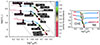 |
Fig. 1. Left: Hertzsprung–Russell diagram summarizing the findings of Paper II (their Fig. 1 & Table 4) and our Sect. 2.2, showing that chemically homogeneous stellar evolution at I Zw 18 composition proceeds from class O via a shorter-lived class WN to a longer-lived WO phase – i.e. without experiencing any long-term WC phase. Evolutionary models are taken from Paper I (main-sequence) and Szécsi et al. (2022, post-main-sequence), without correcting for the wind optical depth (see the last paragraph of Sect. 2.2). Initial masses are labelled, showing where the tracks start their evolution, which proceeds towards the hot side of the diagram (i.e. CHE). Colours show the central helium mass fraction, and dots represent every 105 years of evolution. Dashes mark equiradial lines with 1, 10, and 100 R⊙ from left to right. The black star symbols represent the models for which PoWR synthetic spectra were computed in Paper II and Sect. 2.2. From right to left (note that the evolution progresses from red to blue, contrarily to classical massive-star evolution): main-sequence models with surface helium mass fractions of 0.28, 0.5, 0.75, and 0.98, while the fifth symbol on the very left corresponds to the core-helium-burning phase (post-main-sequence, Sect. 2.2). Spectral classification was performed in Paper II; the results (for four different assumptions about mass loss and clumping) were presented in their Table 4 and Appendix A. Here the labels summarize the ranges in class found there, except for the WN and WO stars which are discussed in Sect. 2.2 (see also Fig. 3). Right: HR diagram summarizing our findings from Paper I. Stellar models computed with I Zw 18’s chemical composition are shown following normal evolution (NE) towards the red supergiant branch with slow rotation (≲300 km s−1). With fast rotation, they are seen following CHE towards hot surface temperatures; that is, leftward from the ZAMS. This latter evolutionary path is what is elaborated upon in the left panel. For more details on how we construct a synthetic population out of both these kinds of models, see Sect 2.3. |
The spectra published in Paper II were created for three masses (Mini = 20, 59 and 131 M⊙, all with a high initial rotational rate of 300–600 km−1), five evolutionary stages (four on the main-sequence and one post-main-sequence, see also Sect. 2.2), two mass-loss rates (a nominal one taken from the evolutionary models, and a reduced one; actual values listed in Table 2 of Paper II) and two types of assumptions about wind clumping (a smooth wind and a clumped wind with clumping factor D = 10). The mass-loss rate values are supported by those that Hainich et al. (2015) empirically predicted for the same stars. Additionally, more realistic mass-loss rates of these stars were calculated by Abdellaoui (2023) using the VH-1 code, which allows for a multi-dimensional treatment of the wind. The obtained results (listed in their Table 6.3) are somewhere between our nominal and reduced values.
Fig. 2 shows the spectral energy distribution (SED) of some of our models (those with nominal mass-loss rates and smooth wind), as well as the corresponding black body spectrum for context (without applying wind optical depth correction from Langer 1989). As Fig. 2 attests, the SED of these stars do not follow the distribution of black body radiation, even though the total amount of ionizing photons in the three main ionizing continua (Lyman, He I and He II continua) are on the same order of magnitude as in the (uncorrected) black body.
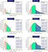 |
Fig. 2. Spectral energy distributions of our PoWR synthetic spectra of chemically homogeneously evolving massive stars published in Paper II with the corresponding black body distributions overplotted for context. The models correspond to the second (MS) and last (pMS) phases on the HR diagram in Fig. 1; their main physical parameters and ionizing fluxes are listed in Table B.1. Titles indicate the initial mass of the evolutionary models with the actual mass (i.e. the mass when the synthetic spectra were computed) in parenthesis. The three main ionizing continua (Lyman: < 912 Å, He I: < 504 Å, He II: < 228 Å ) are marked (note the X scale showing the frequency instead of the wavelength, in order to spread out the relevant high-energy parts of the distributions). Framed boxes present the number of ionizing photons predicted by both the PoWR models (unclumped, with nominal mass-loss rates) and the black body distributions, in units of log(s−1); the values being close to each other is an interesting coincidence. Left column: Models in the main-sequence (MS) phase with surface helium mass fraction of YS = 0.5. Right column: Models in the post-main-sequence (pMS) phase (in the case of the 131 M⊙ model, the late-pMS phase, see Sect. 2.2 and Fig. 4). Note the order of magnitude difference in the Y scale between the left column and the right column. |
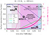 |
Fig. 3. Time evolution of surface properties of the evolutionary model with Mini = 131 M⊙ after the terminal-age main sequence (TAMS). Reproduced from Szécsi (2016, their Fig. 4.13), adding information about our three post-main-sequence PoWR models scrutinized in Sect. 2.2 and Fig. 4. Black star-symbols mark their positions on the central helium mass fraction: YC = 0.8 (early), YC = 0.5 (mid), YC = 0.1 (late). The rudimentary classification of Szécsi (2016, see their Sect. 4.5.1, based on Georgy et al. 2012) is surpassed by the spectral-line-based classification scheme (see also Fig. 4 showing all the optical emission lines), meaning that chemically homogeneously evolving stars at I Zw 18 metallicity do not spend significant time in the WC phase, proceeding from their main-sequence O-star phase to WN and then directly to WO. |
Having these models allows us to build a synthetic population that includes spectral synthesis of various emission lines. Before we do that (Sect. 2.3), we present two new model spectra to properly account for the post-main-sequence, a phase crucially relevant for our goals.
2.2. New PoWR spectra: WN and WO stars (no WC)
In our Paper II, the post-main-sequence phase was accounted for by models with central helium mass fraction of YC = 0.1; that is, nearly the end of core-helium burning. The spectra were classified as type WO according to the standard spectral classification scheme (for details on this, see Table 4 & Appendix A of Paper II, as well as our Fig. 1), and showed very prominent emission lines in both the optical and the UV regimes. However, according to Figure 3, the evolutionary model predicts significant change in the surface abundances while core-helium burning is in progress, with the YC = 0.1 stage being quite different from earlier times. Therefore, before using these late-stage models in our population synthesis (Sect. 2.3), we should justify the extent to which they are representative of the entirety of the post-main-sequence, and discuss their evolutionary behaviour and spectral classification.
To this end, we computed two more spectral models using PoWR for YC = 0.8 and YC = 0.5 of a very massive star with initial mass Mini = 131 M⊙ (actual mass around 93−106 M⊙, see the caption). The computational set-up was the same as in Paper II. We apply nominal mass-loss rates taken from the evolutionary model (Szécsi et al. 2015, 2022; Szécsi 2016), and smooth winds (clumping factor D = 1); we discuss in Sect. 5.2 that these assumptions are actually quite robust. Figure 4 compares the optical band for these spectra, while Figure 3 summarizes what we learned in terms of stellar classification.
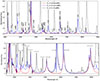 |
Fig. 4. PoWR model spectra of individual stars during the post-main-sequence (core-helium burning) phase of the same evolutionary model (Mini = 131 M⊙, actual mass between 93−106 M⊙). The model’s approximate position is shown on the HR diagram in Fig. 1 by the last point (pMS phase) at around log(Teff/K) ∼ 5.14 and log(L/L⊙) ∼ 6.7. Top: Optical range. Bottom: UV range. Nominal mass loss rate and no clumping was assumed, to be consistent with previous work (see Paper II, and the discussion of the caveats in Sect. 5.2). YC indicates core-helium abundance and thus the evolutionary progress during the post-MS. The earliest model (red straight line, YC = 0.8, i.e. just burned about 20% of its helium in the core) shows prominent emission only in helium, while the mid (blue straight line, YC = 0.5) and late (black straight line, YC = 0.1, corresponding to the bottom right panel of Fig. 2) ones develop carbon and oxygen lines too. (The Cl and S lines are modelling side-effects, we do not expect them to show up in observations.) However, the distinguishing emission line C IIIλ5696 Å which serves as the basis of classifying a stars as WC (Crowther et al. 1998) is missing in all three models. So are the nitrogen emission lines that would categorize a star as late-type WN (Crowther et al. 1995; Smith et al. 1996; Crowther & Walborn 2011). If observed, therefore, these stars would be identified as early-type WN (i.e. WN2) and then during most of the core-helium burning, as WO – more precisely, WO 2 evolving to WO 1. |
Applying the rudimentary scheme of classification defined by Georgy et al. (2012) for evolutionary models, Szécsi (2016, in their Sect. 4.5.1) suggested that these stars are of the classes WN, WC, and close-to-WO, respectively (Fig. 3). However, the PoWR spectra tell a different story. The standard classification scheme (working with spectral line intensity2 as summarized by Appendix A of Paper II) yields the following classes: WN2 for YC = 0.8, WO 2 or WO 1 (consistent with both) for YC = 0.5, and WO 1 for YC = 0.1. Based on what we learned in Paper II (especially their Figs. 4 and B6), we expect that reducing the mass loss rate and/or increasing the wind clumping may shift these spectra towards different subtypes – that is, towards different line intensities – but not towards a different class. In other words, varying mass loss and clumping will not make any of these models a WC star.
We conclude therefore that chemically homogeneously evolving stars at I Zw 18 metallicity would be seen, after spending their main-sequence as O stars, as early-type WN stars at the beginning, and WO stars in the majority of their post-main-sequence lifetimes. This is surprising since typical evolution calculations for single stars predict the WO stage to be a rather late, short-term phase, preceded by a lengthier WC phase (see e.g. Groh et al. 2014), the typical sequence of classes reading:

Chemically homogeneous evolution does not follow that picture, as these stars complete their main-sequence as very hot O stars (Sect. 2.1 and Fig. 1) and then proceed to be WN and WO after that, a completely new sequence of classes:

According to Fig. 3, if a WC-phase arises at all between WN and WO, it will not last longer than about ∼1–2% of the total stellar lifetime.
Finding our stars to be WO instead of WC is in accordance with Tramper et al. (2013) who concluded that WO stars may be the high-temperature and high-luminosity extensions of WC stars. The WO spectral type does not necessarily mean more oxygen than carbon: in our mid-pMS model, the carbon abundance is actually higher than the oxygen one (as is seen in Fig. 3). The same was found for the LMC WO stars analysed in Aadland et al. (2022). So it is not about abundance but about temperature: carbon is ionized into C V and thus the otherwise prominent 1550 and 5808 features are weak or absent.
While WC and WO may not necessarily represent different evolutionary stages from a theorist’s point of view, for an observer the distinction could be important. The label “WO” is a spectral classification, hence we keep using it here. As is seen in Sect. 4, the detected features of I Zw 18 are consistent with WO stars.
Nevertheless, the three phases do not differ much when it comes to the SED, yielding log QHe II values of 49.80 (early-pMS), 49.79 (mid-pMS) and 49.79 (late-pMS). Note how the surface temperatures of the evolutionary models are similar: the Teff of the early-pMS model is 138.9 kK, mid-pMS 139.2 kK, and late-pMS 138.0 kK (see Fig. 1 where the burning is colour-coded). In terms of atmosphere models, Teff roughly reflects the wind onset region where τ = 20; but even T2/3 (i.e. T at τ = 2/3) is close for the three cases (with early-pMS 56.6 kK, mid-pMS 63.3 kK, late-pMS 70.3 kK), explaining why the predicted He II flux is not changing considerably during the core-helium burning phase. Thus, using late-pMS models in our population synthesis to stand for the entirety of the post-main-sequence is well justified when it comes to the ionizing photon count.
As for emission-line intensities, the mid- and late-pMS models (both WO) predict LC IV = 2.13 · 1037 erg s−1 and 3.77⋅1037 erg s−1, respectively. Since clumping introduces a factor of 3 uncertainty (as is shown in Fig. 6), our use of the late-stage value to represent the entire post-main-sequence is justified with the caveat that winds are probably not unclumped (see Roy et al. 2025) and that the observational range we attempt to match (L = 2.2–5.5⋅1037 erg s−1) itself includes such an error margin.
2.3. Population synthesis
Equipped with all these model spectra, we now revisit the question of photoionization in I Zw 18 by building a syntheticpopulation of metal-poor massive stars. Since chemically homogeneous stars (TWUIN or O/WN/WO) are a straightforward outcome of rotating stellar evolution at the metallicity of I Zw 18, these stars are automatically included.
It was shown in Paper I that a population of single metal-poor massive stars on the main sequence is able to explain I Zw 18’s He II ionizing flux (Paper I, Sect. 10.4). No other observable was investigated in that simple population calculation. Further assumptions were (i) a Salpeter-type initial mass function (IMF); (ii) ongoing star formation for the past 3 Myr with a rate of 0.1 M⊙ yr−1 (this rate was observed by Lebouteiller et al. 2013) resulting a 300 000 M⊙ total mass in the region; (iii) an upper mass limit set to 500 M⊙; (iv) a rather high fraction, ∼20% of stars rotating fast enough to evolve chemically homogeneously and therefore becoming TWUIN stars (instead of cool, non-ionizing supergiants); and (v) black body emission3.
We revise these assumptions here. Most importantly, we included the full evolution, i.e. both the main- and the post-main-sequences of our stellar models. We still used a regular Salpeter IMF (Salpeter 1955) for a continuous star formation episode lasting for 3 Myr forming 0.1 M⊙ yr−1, same as before. The upper mass limit was, however, set to a more realistic 150 M⊙ (as opposed to 500 M⊙; though note that even 200 M⊙ might be acceptable in light of Bestenlehner et al. 2020). The ratio of chemically homogeneously evolving stars was also relaxed: 10% now (as opposed to 20%), which is better supported by the rotational velocity distribution measured in the Small Magellanic Cloud (1/5 Z⊙, Mokiem et al. 2006), where about 10–15% of massive stars rotate faster than what is needed for CHE at the ten times lower metallicity of I Zw 18. This means that, in the population we built here, 90% of the massive stars are in fact ‘normal’, slow-rotating stars, i.e. not chemically homogeneous, but classical single stellar evolution leading to O/B stars and supergiants. No classical WR stars though, as at this metallicity the supergiants do not lose their complete envelopes in the rather weak stellar winds, as is shown by Szécsi (2016), Szécsi & Wünsch (2019), Szécsi et al. (2022). These ‘normally’ evolving O/B stars are taken into account assuming black body emission: their contribution to the ionizing flux is only significant near the zero-age main sequence (ZAMS) when they are the hottest, while they do not contribute to emission line luminosities, for even in their early lives they are less hot than their chemically homogeneously evolving counterparts (as is seen in Figure 1, right panel); thus, they surely experience transparent winds and absorption-type spectra. We include low-mass stars (< 9 M⊙) only as mass holders down to 0.5 M⊙, the same way as in Paper I.
To account for the radiation field emitted by the chemically homogeneously evolving TWUIN/WO stars, we used the SED predicted by our synthetic spectra from Paper II with a nominal mass-loss rate and smooth wind (Fig. 2). This way there is no need to correct for wind optical depth. Such a correction is a common practice for evolutionary models, done in for example Groh et al. (2019), Schootemeijer & Langer (2018), and Szécsi (2016). They followed the estimates of Langer (1989), which took only electron-scattering opacity into account: a fast but simplistic method. Since our spectra were created with state-of-the-art physical treatment of all elements in PoWR, including the high ionization stages of iron group elements (albeit with reduced abundances corresponding to the low metallicity), all sources of opacity are taken into account.
As the spectra in Paper II are only provided for three initial masses, we linearly interpolated between the predicted flux values to get a smooth distribution. This is shown in Figure 5. The most massive stars’ post-main-sequence phase (spectral type WO) provides the largest ionizing photon count. So even if such stars are rare according to a typical IMF, their contribution to the He II ionization can be significant. Yet, the population synthesis includes the contribution of all the hot O-stars, as explained above. It depends on the star formation history (see Sect. 3) whether very massive stars would form and dominate over the population or not. In either case, the ratio of WR/O stars in our synthetic population is around 0.001, which is consistent with the lowest-Z observations (upper limits) of López-Sánchez & Esteban (2010a, their Fig. 5).
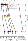 |
Fig. 5. Top panel: Number of ionizing photons in the He II continuum in all our spectral models from Paper II. Evolutionary stages are indicated by colours (ZAMS by yellow; two main sequence models with surface helium mass fractions YS = 0.5 and 0.75 by green and red, respectively; terminal-age-main-sequence model, TAMS, by blue; and post-main-sequence model, pMS, by purple). For every evolutionary stage, QHe II from all four spectral models of Paper II are shown (hence the spread in the coloured stripes). Yellow circles represent the He II ionizing photon number computed from corresponding black body distributions (see Fig. 2). To account for a population of massive stars, we interpolate linearly between the logarithm of the three simulated masses. Models with nominal mass-loss rate and unclumped wind are used; interpolated values are shown with the solid black lines, small triangles marking the bin sizes. Above and below our highest and lowest mass models, the values of those models are applied (down to 9 M⊙). Bottom panel: Same as the top panel, but for the line luminosities in C IVλ1550 Å of the pMS model. The second trio of pink rectangles with higher values correspond to clumped wind models (see also Fig. 6). Other line luminosities are treated the same way (see Sect. 2.4). |
To sum up, all our assumptions about the synthetic population are either less extreme than those in Paper I or identical, while the models we apply are more elaborate. Our results, including further parameter studies, are reported and compared to observational data in Sect. 3.
2.4. Luminosity in emission lines
We performed spectral synthesis for emission lines by computing the line luminosity from our spectra. Figure 6 shows an example: the flux around 1550 Å is plotted for the models where the C IV line is in emission (that is, post-main-sequence models with a nominal mass-loss rate).
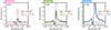 |
Fig. 6. Normalized flux around the UV line C IVλ1550 Å in three post-main-sequence (l-pMS) spectral models with initial masses as indicated in the top left corner of the panels. Line luminosity (computed following Sect. 2.4) is given in the framed boxes in units of log(erg s−1); lg L stands for unclumped (clumping factor D = 1) while lg Lcl for clumped (D = 10) wind, see details in Paper II. When creating the synthetic population here (Sect. 2.3 and Sect. 3.1), we always apply the unclumped models’ predictions (i.e. black line). Other emission lines are presented in Figs. A.1–A.2. Based on this, we predict a ∼40–50 Å-wide emission bump from our population between 1550–1600 Å, which is indeed present in the observations in Fig. 11. |
The C IVλ1550 Å emission line luminosity depends strongly on the mass-loss, meaning it depends on the mass of the model: for the Mini = 20 M⊙ model (the mass of which is only 17 M⊙ in the post-main-sequence phase; there is mass-loss over the evolution) it is in the order of 1035 erg s−1, while for our very massive model of Mini = 131 M⊙ (post-main-sequence phase mass only 95 M⊙) it is in the order of 1037 erg s−1. Although we focus on the models with smooth wind (i.e. without wind clumping) in this work, Fig. 6 attests that clumped winds at the same mass-loss can increase the line luminosity by almost an order of magnitude.
Interpolation between the C IVλ1550 Å line luminosities is presented in Fig. 5. Population synthesis was done on these values according to the assumptions made in Sect. 2.3. Other emission line luminosities, both UV and optical, were treated the same way.
3. Comparing theory to observations
3.1. Ionizing He II emission and C IV line luminosity
Table 1 summarizes our results. From our fiducial population built in Sects. 2.3–2.4, we predict a total He II ionizing flux of QHe II = 1.80⋅1050 photons s−1 and a total C IVλ1550 Å emission line luminosity of L1550 = 3.71⋅1037 erg s−1. These are not far from what is measured in I Zw 18: Q = 1.33⋅1050 photons s−1 and L
 = 2.2–5.5⋅1037 erg s−1 (see Sect. 1)4. Translating our statistics-based predictions into number of stars, we get about one or two post-main-sequence chemically homogeneously evolving objects – that is, WO stars (see Sect. 2.1–2.2) – of mass > 90 M⊙ in the population. The contribution of these one or two very massive WR type stars is responsible for the C IV line luminosity, while the He II photon emission is coming from them and the rest of the hot-star population (including normally evolving models).
Summary of our population synthesis runs, best match shaded with colour.
There is no need for very massive stars, however, since alternative star formation histories are within reasonable margins of theoretical and observational uncertainties. For example, a continuous episode lasting for 10 Myr with a much more moderate rate of only 0.03 M⊙ yr−1 also results in a 300 000 M⊙ region; this population gives us QHe II = 1.96⋅1050 photons s−1 and L1550 = 3.43⋅1037 erg s−1. We have lowered the top mass value Mtop of the IMF from 150 to 120 M⊙ for this run, because already this more moderate value gives us the right predictions. In this case, the main source of the UV carbon line is made up by six chemically homogeneously evolving WO stars of mass ∼40 M⊙ and another one of mass ∼80 M⊙; while the He+-emission is again explained by the combined contribution of these and the rest of the hot-star population (including those classified as type O in Fig. 1). So instead of a couple of very massive WO stars, a select number of more or less average ones can do the same job.
We can relax our assumptions even further, by applying a 0.02 M⊙ yr−1 rate for a 15 Myr long star formation episode (again with Mtop = 120 M⊙; see Table 1). This way our 20 M⊙ model’s post-main-sequence phase (which hardens the resulting ionizing emission considerably; see Sect. 3.2) would be captured (the model’s total lifetime is 12.3 Myr). In such a scenario, about twenty-three WO stars of 20–25 M⊙ and two of around 50 M⊙ are responsible for a predicted carbon emission of L1550 = 2.83⋅1037 erg s−1 and an ionizing flux of QHe II = 2.19⋅1050 photons s−1. Sect. 3.2 shows that this third scenario is the most preferred in terms of the spectral hardness, a further observational constraint. Table 1 presents a fourth and a fifth scenarios, which are even more moderate in terms of Mtop (80 an 40 M⊙), but they fail to account for the observed C IV luminosity.
As for correcting for extinction, Brown et al. (2002) reported that E(B-V) = 0.06 for an SMC-type extinction law fits the data well. From this one obtains a factor ∼2.3 attenuation at ∼1500 Å. The recent study of Berg et al. (2022) quotes E(B-V) = 0.0753 ± 0.007, which gives a higher correction (∼2.7). With these numbers, one can estimate LC IV ∼ (5−15)⋅1037 erg s−1, which is around the same or up to 3 times higher than the L range we attempt to match here (2.2–5.5⋅1037 erg s−1). However, as Fig. 6 shows, introducing wind-clumping into our models increases our predicted line luminosity significantly – up to 3 times higher values with an extreme clumping factor. As is explained in Sect. 5.2 among caveats, wind-clumping is one of the most underconstrained parameters of massive-star atmospheres, and supposing that the winds are completely unclumped (i.e. smooth) is a rather conservative assumption (see also Roy et al. 2025).
We conclude therefore that a population of metal-poor massive single star models – including those with fast rotation that evolve to be TWUIN stars – can successfully explain the puzzling properties of the very dwarf galaxy, I Zw 18, which they were created for. The emission is dominated by WO stars, with a total C IV emission line intensity around 2−3⋅1037 erg s−1.
3.2. Nebular line ratios versus continuum photon ratios
The number of ionizing photons in I Zw 18 was obtained from measuring the strength of the line He IIλ4686 Å which originates in the ionized interstellar nebula. Kehrig et al. (2015a) report a line luminosity of 1.12⋅1038 erg s−1 from which they derive Q using common assumptions about the interstellar medium’s properties. An important observable to investigate is how the ratio of He II photons to Lyman continuum photons relate to the observed line intensities of the corresponding, excited nebular lines, He IIλ4686 Å and H[[INLINE428]]λ4861 Å. Observationally, this hardness ratio is measured to be in the range of I(4686)/I(H[[INLINE429]]) = 0.02−0.04 (Izotov & Thuan 1998; Lebouteiller et al. 2017, although Kehrig et al. 2015a report values as high as 0.08 in individual spaxels). From a theoretical population of massive stars, one can predict this ratio as I(4686)/I(H[[INLINE432]]) = A⋅Q(He II)/Q(H I), where A is a factor taken to be 1.74 for typical nebular conditions (Stasińska et al. 2015).
In our fiducial population (containing not just WO stars but all hot stars, including O-type stars from ‘normal’ evolution; see Sect. 2.3), the predicted photon count is Q(H I) = 7.02⋅1052 s−1 in the H I continuum (as reported in Table 1) and Q(He II) = 1.80⋅1050 s−1 in the He II continuum. From these, we derive the hardness ratio to be 0.004 (Table 1), which is an order of magnitude below what is observed (0.02–0.04).
However, for the alternative populations, when lower-mass stars are captured by relaxing the length of the starburst (Sect. 3.1), the value rises to 0.011 and 0.017, approaching the expected range. From this we deduce that the extremely short and intense scenario suggested by Paper I (our fiducial population) where a couple of very massive stars dominate the emission is rendered unlikely. Instead, a population where all massive stars’ post-main-sequence phases are contributing, not just the youngest (very massive) ones, should be considered realistic. In our second scenario (SF-10 in Table 1) the age of the starburst excludes post-main-sequence objects with initial masses below ∼30 M⊙, while in our third scenario (SF-15 in Table 1), everything down to ∼20 M⊙ is incorporated. The contribution of this evolutionary model to the hardness of the population is demonstrated by Figure 7, where evolutionary sequences are compared in terms of their (black-body-estimated) ionizing emissions. We suggest that in the future, PoWR models down to 12 M⊙ could be computed and tested for their effect of increasing the hardness – an apparent trend – fitting the observed range even better.
 |
Fig. 7. Hertzsprung–Russell diagrams with background colours representing the number of Lyman (left) and He-II (right) continuum photons emitted by a black body with a given temperature and luminosity. Units are associated with colours (pink: 1048 ph s−1, blue: 1049 ph s−1, green: 1050 ph s−1, #FAF2BF;: 1051 ph s−1; a black background means < 1048 ph s−1). Stellar evolutionary model sequences are labelled with their initial masses. They are taken from the BoOST project (Szécsi et al. 2022), except for the turquoise line, which is a stripped binary model from Götberg et al. (2017). White lines mean Milky Way composition, where all models evolve the ‘normal’ way (although the most massive ones turn to the left eventually: this is classical Wolf–Rayet evolution). Purple and golden lines mean I Zw 18 composition, with one of the very massive models evolving normally (initial rotational velocity of 100 km s−1) and the others chemically homogeneously due to fast rotation (500 km s−1). Every 105 yr of evolution is marked with dot on the tracks. Including the 20 M⊙ model into our population synthesis runs (with a sufficiently long star formation episode, see Table 1) hardens the combined spectra considerably (reaching close to the observed I(4686)/I(β) ∼ 0.02), as the late phases of this model enter the pink zone in terms of He-II photons while not leaving the blue zone in terms of Lyman photons. For more details on the population synthesis and spectral hardness, see Sects. 2.3 and 3.2, respectively. |
Since lowering Mtop from 150 to 120 M⊙ helped us match the measured hardness, we checked even lower values, down to 80 and even 40 M⊙. They give less good matches: the general trend is that lowering Mtop does not influence our He II and hardness predictions at all (at least as long as the 15 Myr star formation history is applied), but the C IV line luminosity decreases below the observed range.
We conclude that our theory is consistent with the measured hardness in I Zw 18, and by matching this value as an additional constraint we can draw important conclusions on the length and intensity of the starbursts, as well as the stellar content, favouring less violent and more relaxed scenarios over those dominated by very-massive stars.
4. Available observations in the literature
Apart from the C IVλ1550 Å line and the continuum photons, there are further observational features our results should be consistent with. To make such a comparison, we review here the published spectral data of I Zw 18 focusing on individual emission lines and bumps. The figures below (Figs. 8–13) are reproduced from the literature for the sake of this discussion. Table 2 lists the papers, instruments and spectral ranges (optical or UV) mentioned here. As we shall see, paying attention to the observing strategy of any given survey is key before drawingconclusions.
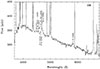 |
Fig. 8. Optical spectra reproduced from Izotov et al. (1997, their Fig. 1). Spectrophotometric observations were obtained by the MMT Observatory using a 1 |

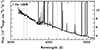 |
Fig. 9. Optical spectra reproduced from Thuan & Izotov (2005, their Fig. 2). Observation taken with the MMT spectrograph (blue channel) at the 6.5 m MMTO. A 2″ × 300″ slit was used, and the brightest part of the north-western H II region was extracted using a 6″ × 2″ extraction aperture. For our discussion, see Sect. 4.1. |
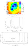 |
Fig. 10. Optical spectra reproduced from Kehrig et al. (2016, their Figs. 2 & 6, here top & middle, respectively) and Kehrig et al. (2015a, their Fig. 3, bottom). Integral field spectroscopy was obtained with the Potsdam Multi-Aperture Spectrophotometer (PMAS) on the 3.5 m telescope at the Calar Alto Observatory (Almeria, Spain). Top: Hβ map with a cross marking where the spectrum in the middle was extracted from. Middle: Spectrum showing a prominent WR-bump associated with stellar emission underneath the narrow, nebular He IIλ4686 Å line, discussed in Sect. 4.1. Bottom: Integrated spectrum of the north-western region of I Zw 18, demonstrating how stellar emission bumps clear out completely when the full galaxy is integrated over, leaving only the narrow nebular component. Compare this to the FUSE data in Fig. 12, which we discuss in Sect. 4.2. |
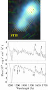 |
Fig. 11. UV spectra reproduced from Brown et al. (2002, their Fig. 1). Observations taken with Hubble’s Space Telescope Imaging Spectrograph (STIS) using the G140L grating and the 52″ × 0 |

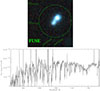 |
Fig. 12. UV spectra reproduced from Lecavelier des Etangs et al. (2004, their Fig. 1). Observation taken with FUSE, with an aperture (30″ × 20″) covering the whole galaxy. Top: Position of the observation; picture is taken from the MAST archives with background image from Pan-STARRS. Bottom: Spectra presented in Lecavelier des Etangs et al. (2004). Since the full galaxy is in the aperture, the features of the localized stellar populations are not expected to be seen (see Fig. 10, as well as our discussion in Sect. 4.2). |
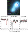 |
Fig. 13. UV spectra reproduced from Heap et al. (2015, their Fig. 5). Top: Regions of the Hubble COS observations according to the MAST archive (PI: J.C. Grean, year: 2010, aperture: 2 |

Summary of the various measurements from the literature reproduced and discussed here.
We remind the reader that our best fit population predicts ∼LC IV = 2.83⋅1037 erg s−1 (coming from twenty-something WO stars between 20–50 M⊙). This is actually close to what our newly computed PoWR model (with 131 M⊙ in the mid-pMS) predicts (2.13⋅1037 erg s−1). Therefore, to ease the following discussion, we simply consider this mid-post-main-sequence model (blue line in Fig. 4) representative of the combined spectrum of the population.
4.1. Optical emission lines (bumps)
4.1.1. O VI λ3818 Å.
There are two observations available in the literature for this spectral region, Izotov et al. (1997) and Thuan & Izotov (2005). The first is reproduced here in Fig. 8 and the second, in Fig. 9. According to our model spectra in Fig. 4, this emission is predicted to be not a line but a huge double bump, ranging from 3780−3850 Å (see also Fig. A.1 showing our line predictions). In the Izotov et al. (1997) spectra (Fig. 8), the flux calibration seems to be off at the position in question (it suddenly drops at the edge) making it hard to tell whether a broad component is there or not. The second paper, Thuan & Izotov (2005), did not report detection of the O VIλ3818 Å line (see their Table 3), which is consistent with what one sees looking at Fig. 9. However, the Thuan spectra also do not show the blue bump centred at λ ≈ 4650 Å that is so prominent in the Izotov spectra. Thus, seeing other wide bumps of stellar origin should not be expected in the Thuan data, either. We conclude that the currently available literature does not exclude our model predictions about this emission bump.
4.1.2. He II λ4686 Å.
This optical line is peculiar because it may have a stellar and a nebular component. The nebular one is narrow, the stellar (if there) broad, bump-like: our theory predicts a wide double bump between 4640–4700 Å (Fig. 4) that should be about as prominent as the C IV bump around 5808 Å. The Izotov et al. (1997) spectra therefore supports our theory: a bump is clearly there in Fig. 8 under the narrow nebular component. The same is true for the spectra presented in Kehrig et al. (2016), shown here in Fig. 10. As for Thuan & Izotov (2005), they measure an equivalent width of 2.5 Å (their Table 3) for the nebular line; whether there is a 60 Å-wide, almost completely cleared-out bump of stellar origin underneath it (Fig. 9), it is hard to say. We speculate that the lack of stellar emission bumps in the Thuan data may be attributed to the extraction aperture (6″ × 2″) not crossing over the star clusters of interest, while the aperture of the Izotov data (5″, centred on the north-western region) includes these regions. Indeed, the position and size of the extraction apertures may play a key role in the detection of (or lack of) spectral features, as demonstrated by Kehrig et al. (2013, see their Fig. 11). We conclude that the existing literature does not exclude our model predictions about this line.
4.1.3. C IV λ5808 Å.
Only the Izotov et al. (1997) observation covers this region (Fig. 8). This measurement does show a bump at 5808, thus supporting our theory. Even the relative strength of it compared to the above discussed He IIλ4686 Å bump is tentatively consistent with our predictions in Fig. 4.
4.1.4. C IV λ7724 Å.
We did not found any spectra in the literature covering this wavelength.
4.2. UV emission lines (bumps)
4.2.1. He II λ1640 Å.
The appearance of this UV emission line (bump) is crucial, as it is typically used as a proxy for first stars (Pop-III). However, there are other ways to produce this line, as our models (massive Pop-II stars) attest. The bump is visible in the HST STIS spectra of Brown et al. (2002), as is seen in Fig. 11, and its size is comparable to that of the C IVλ1550 Å bump. Our theoretical populations nicely account for this. We predict line luminosities of lg L = 37.58 for C IV (see Fig. 6) and lg L = 37.35 for He II (see Fig. A.2) in the case of our mid-post-main-sequence WO model that dominates the population. As for the alternative population where a select number of more moderate-mass models dominate (see Sect. 3.1), the situation is similar: the values the WO star with Mini = 59 M⊙ gives are lg L = 36.82 for C IV and lg L = 36.63 for He II. Thus, this UV emission line supports our theory. We note however that when attempting to repeat the data reduction (the observations are publicly available in the MAST archive5) we found it challenging to identify the prominent bumps reported by Brown et al. (2002). While reanalysing archival HST data is outside the scope of the current work, we encourage ongoing projects (e.g. S. Heap, private comm.) in this direction.
4.2.2. O VI λ1037 Å.
This UV line is even stronger in our model spectra than C IVλ1550 Å (see Figs. 4 and A.2). Hence, we should look for it in the observations. Brown et al. (2002, Fig. 11) do not cover the position of O VIλ1037 Å, unfortunately. Other works, such as Lecavelier des Etangs et al. (2004) do, although without covering C IVλ1550 Å, as is seen in Fig. 12. However, the observational strategy is again an important factor. Brown et al. (2002) took their UV spectrum as a slit crossing through the star-forming region in the north-western cluster (see their Fig. 1 where they show their slits on the detailed map of I Zw 18, as well as our less detailed Fig. 11 where we show the same). Lecavelier des Etangs et al. (2004) applied another strategy: the FUSE aperture they used covers the full galaxy (30″ × 20″), as is shown in Fig. 12. In this integrated spectrum, a stellar emission in O VIλ1037 Å is not necessarily expected to be seen – the same way stellar emissions in the optical are not seen in the integrated spectrum presented by Kehrig et al. 2015a: the 4650 bump, otherwise identifiable in targeted observations (e.g. Izotov et al. 1997, see Fig. 8) is completely cleared out when the data is summed over, as is shown by Fig. 10 (reproduced from Fig. 3 of Kehrig et al. 2015a). Still, one might identify a P-Cygni profile around O VI1032 in the FUSE spectrum, just as we predict (see Fig. A.2). We conclude that the available data in the literature does not exclude our model predictions about this line.
4.2.3. C IV λ1169 Å, C III λ1175 Å, O IV λ1340 Å, O V λ1371 Å.
These lines are mentioned in Heap et al. (2015) who presents Hubble’s Cosmic Origins Spectrograph (COS) observations for them (their Fig. 5, reproduced here as Fig. 13). Since emission seems to be absent in their standard fit, they conclude that, the ultraviolet spectrum of [the north-western region] shows no evidence of extremely hot, luminous stars”. The same conclusion was arrived at by Berg et al. (2022), after analysing the highest signal-to-noise-ratio UV spectrum of I Zw 18 available to date, taken by COS/HST (and incorporated in CLASSY). However, the observational strategy is again important here. As Fig. 13 shows, the COS field of view extends to a substantially large fraction of the north-western region, as opposed to using slits crossing through the sources of interest (similarly to the STIS data, see Fig. 14 for a direct comparison). As is demonstrated by the integral-field-spectroscopy results of Kehrig et al. (2016, which we discussed in Fig. 10), emission bumps of stellar origin are only visible when the spectrum is extracted from the right spatial position where those massive stars (star clusters) are physically located. When the entirety of the light is integrated over, the stellar emission clears out (Fig. 10, bottom). Therefore, we the fact that the COS data show no stellar emission bumps does not necessarily mean that those stars are not there. It may simply mean that the COS aperture is too large to detect them, and more targeted campaigns are needed. We conclude that these observations do not disprove our theory either.
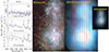 |
Fig. 14. HST measurements of I Zw 18. The panel labelled MAST/Pan-STARRS shows the circular aperture used for obtaining the highest signal-to-noise-ratio UV spectrum of I Zw 18 available to date, taken by COS (Berg et al. 2022). Circle and background image are the same as in Fig. 13 (taken from the MAST archive applying background image from the Pan-STARRS survey). The panels to the left correspond to STIS copied from Brown et al. (2002, mentioned also in Sect. 4.2 and Fig. 11, see details there). The positions where Brown et al. (2002) identified WR-like emission bumps (c and d) are marked by Xs for convenience. The panel labelled MAST/DSS demonstrates a discrepancy we found in the MAST Archive’s AstroView tool (see Sect. 4.3 for details). Our explanation for why the COS spectrum analysed by Berg et al. (2022, see their Fig. 12) does not display C IV emission – despite at least one of the Brown-sources seemingly being within the aperture – is that the field of view includes too much contaminating light: as demonstrated by Kehrig et al. (2016) using integral field spectroscopy of I Zw 18 (see our Fig. 10), stellar emission bumps clear out completely unless the spectra is taken from the right physical position of the galaxy. |
4.2.4. O VI λ2070 Å.
We did not found any spectra in the literature covering this wavelength.
4.3. Using MAST AstroView
While conducting this literature review, we have found a discrepancy in the AstroView tool of the MAST Archive. As is shown by Figure 14, the two available backgrounds give strikingly different visuals at the position of I Zw 18 (RA ∼ 09:34:02, Dec ∼ +55:14:31). While the COS aperture’s position is the same, the DSS background (default option) is off by ∼4 arcsec compared to the Pan-STARRS background (alternative option in the AstroView settings). This can easily lead to confusion when interpreting the COS data (or any other measurement).
According to the MAST Team (Y. Li, private comm.), the Pan-STARRS version is more accurate, although they have not confirmed this to be always true. They hope that these image products will be improved in the future, and they do not recommend using them for scientific analysis, only for preview. While for our present purposes, such previews are quite enough, this is a warning to the community that discrepancies of a few arcseconds can be expected when it comes to I Zw 18 and these images. For proper studies, coordinates from recent reference catalogues such as Gaia and Pan-STARRS1 should be used to confirm the accuracy of the galaxy’s – and especially its various regions’ – celestial positions.
4.4. Summary of the literature review
As is seen from this careful analysis of the literature – paying close attention to the observational strategies such as which apertures were used for which measurement – the currentlyavailable data either support, or at least never exclude, our theoretical predictions. Even the Brown data, which claims the presence of WC stars, do not exclude the possibility of these being, in fact, WO stars: the O IVλ1340 Å and O Vλ1371 Å bumps are actually visible in their STIS spectra in Fig. 11. Our models predict these lines to be nowhere near as relevant as for example C IVλ1550 Å or He IIλ4686 Å (Figs. 4 and A.2), which is exactly what we see in the Brown spectra. We conclude therefore that our suggestion about chemically homogeneously evolved WO stars being responsible for the emission bumps so far associated with WC stars is consistent with all available observations of I Zw 18.
5. Discussion
5.1. Other possible explanations
The suggestion that nearly metal-free, hot massive stars (Pop III-like) are responsible for the He II emission in I Zw 18 (Kehrig et al. 2015a,b; Heap et al. 2015) is certainly appealing, but relies on the galaxy keeping (or obtaining) pockets of primordial gas that have just recently started to form massive stars for some unclear reason (see the review of Klessen & Glover 2023 claiming that Pop III star formation ended roughly at z ∼ 5). Our scenario follows more straightforwardly from the present day conditions in I Zw 18. Our stellar evolutionary models were computed with the measured composition of the very dwarf galaxy we study (following the gas composition reported in Lebouteiller et al. 2013), while our synthetic spectra were created based on these evolutionary models with the most state-of-the-art physics. The population synthesis is a rather general one, without extreme assumptions. So if metal-poor massive stars behave the way the models predict, then both Q and L
and L are properly accounted for – without needing to postulate the presence of Pop III-like stars. Note that according to the seminal work of Yoon et al. (2012), Pop III stars also evolve chemically homogeneously when rotation is included, the same way as our metal-poor (i.e. massive Pop II) stars do.
As for the scenario proposed by Péquignot (2008), Lebouteiller et al. (2017) and Schaerer et al. (2019) on X-ray binaries, we note that chemically homogeneously evolving stars have been shown to lead to high-mass X-ray binaries in case they are born in a close binary system (Marchant et al. 2017). While Kehrig et al. (2021) refutes that high-mass X-rays binaries and/or diffuse soft X-ray photons would be the explanation for the high-ionizing features in I Zw 18, it may still be true in other galaxies. Hence, we suggest our scenario to be complementary to that of Schaerer et al. (2019), and welcome further research into the direction of combining these two possibilities (e.g. applying the methods developed in Sen et al. 2024 for predicting faint X-ray emissions).
Indeed, while we only use single star models here, massive binaries are able to evolve chemically homogeneously too (e.g. de Mink et al. 2009; de Mink & Mandel 2016; Marchant et al. 2016). Alternatively, they may become analogous to our single, chemically homogeneous stars after losing their envelopes in a mass transfer phase (Götberg et al. 2017). Since double systems may be common in massive stellar populations (Sana et al. 2012; Hainich et al. 2018; Spencer et al. 2018), a more comprehensive picture of the contribution of chemically homogeneously evolving stars to the photoionization and carbon line emission in metal-poor galaxies will need to involve not only our fast rotating single stars (especially since there is ongoing debate on the effectiveness of rotationally induced mixing, e.g. Higgins & Vink 2019), but binaries as well.
As for the model of Oskinova & Schaerer (2022) suggesting cluster-winds emitting X-rays, we note that this again can be nicely reconciled with our models. Indeed, our very evolutionary models have been applied in cluster-wind studies accounting for X-ray emission in green pea galaxies (Franeck et al. 2022). A similar study for I Zw 18 would be, therefore, quite possible, and we foresee a follow-up project combining the ionizing emission from massive stars and their shocked winds.
Roy et al. (2025) recently suggested that classical WR stars with clumpy winds can produce hard photons in local and high-z galaxies. To test this scenario’s validity in I Zw 18, the C IV and other observed emission line luminosities that their models predict would need to be compared to observations. The same is true for the seminal work of Lecroq et al. (2024), in which they build a complex spectral synthesis tool including binary processes and investigate various emission lines (both nebular and stellar) in metal-poor stellar populations. We hope that by compiling existing UV and optical spectra from the literature on I Zw 18 – one of the best-studied dwarf galaxies out there – and by critically discussing this set of data in terms of its capacity to guide modelling efforts (Sect. 4), our work will assist future endeavours like these when testing their predictions directly against I Zw 18.
5.2. Caveats
Caveats in our theory include uncertainties inherent in the simulations (see Sect. 6.2 of Paper II for a detailed discussion on this, as well as Agrawal et al. 2022). Some of the main sources of uncertainty are mass loss, wind clumping and rotational mixing efficiency. Especially mass loss and wind clumping can directly influence the strength of the spectral lines – but not the ionizing flux. For example, reducing the mass-loss rate by two orders of magnitude erases any trace of the carbon emission even in the post-main-sequence phase of our models, as is seen in Fig. B4 of Paper II; however, this has practically no effect on the total number of ionizing photons (see Fig. B1 of the same paper). On the other hand, supposing that winds are clumped has an opposite effect on the emission lines: making them more prominent, as is shown by Figs. 6 and A.1–A.2 while not influencing the SED. This means that if mass-loss rates turn out to be lower then the rather high value assumed here, increasing wind clumping – another unconstrained property (see Roy et al. 2025) – may still lead to the same conclusion, making our results quite robust.
As for the efficiency of rotational mixing, it is a widely studied yet unconstrained parameter in stellar evolution theory (Maeder & Meynet 2000; Meynet & Maeder 2000; Brott et al. 2011; de Mink et al. 2013; Burssens et al. 2023). However, our results are rather robust in this context as well. As is explained in Sect. 2.3, we make the simple assumption that 10% of stars rotate fast enough for CHE (guided by the observed initial rotational-velocity distribution of massive single stars in the SMC). So even if rotational mixing is found to be weaker than in our models, our results would be unchanged as long as 10% of the population follows the chemically homogeneous path.
The same is true for other modelling ingredients that influence stellar evolution (e.g. mass-loss rate prescriptions, convective overshooting, semi-convection, core-envelope coupling): with ∼10% of massive stars in the population evolving chemically homogeneously, either as single stars or binaries6, their spectra will look like how the PoWR models predict: so they will help us explain the peculiar features of I Zw 18.
As was shown recently by the seminal work of Abdellaoui (2023, see their Sect. 6.1.3), fast rotation has a strong effect on stellar winds, as well as on the emergent ionizing fluxes. Including these effects (by recomputing our PoWR models using the mass-loss rates obtained by Abdellaoui 2023) will be part of a future work. To repeat, we do not have any “classically” occurring WO stars in our population (i.e. WOs that got stripped by stellar-wind mass loss) because the evolutionary models we rely on do not predict such strong stellar winds at this low metal content (Szécsi et al. 2015, 2022). All our WOs evolved via the chemically homogeneous route, as explained in Sect. 2.3.
The star formation history of I Zw 18 is not conclusively established (Kunth & Östlin 2000; Papaderos et al. 2002; Izotov & Thuan 2004; Papaderos & Östlin 2012), and indeed it has been debated whether it is a typical dwarf galaxy at all (Aloisi et al. 1999; Guseva et al. 2000; Annibali et al. 2013). For example, the IMF may be top-heavy in starbursts; this would help our case. Still, our result that massive stars of I Zw 18-composition are consistently able to account for two, previously unreconcilable observational characteristics while fulfilling all observational constraints available in the literature, implies that their existence should be supposed – and, therefore, further studied – in other galaxies of this type too. For example, some dwarf galaxies may be different from I Zw 18 not because of the typical evolutionary behaviours of their massive stars, but because their star formation history progressed another way due to, for example, different dynamical interactions with other galaxies (see Christensen et al. 2016), or to different thermodynamic/magneto-hydrodynamic conditions in their interstellar gas (see Hopkins et al. 2011; Seifried et al. 2017; Girichidis et al. 2018; Haid et al. 2019), leading to different rotational velocities (or different binary fraction) in the current massive stellar population. Indeed, to obtain a comprehensive theory of low-metallicity massive stars, one will need to correct for such environmental characteristics when accounting for a larger sample of dwarf galaxy observations (see also the conclusions in Stanway & Eldridge 2019), including any possible contribution of the interstellar medium to the emission lines commonly attributed to stellar origin.
6. Conclusions
We have shown that a population of massive Pop-II stars can consistently reproduce the observationally derived He II ionizing flux and the observed C IVλ1550 Å line luminosity in the dwarf galaxy I Zw 18. The source of the emission bump is a small number of chemically homogeneously evolved WO stars: these, combined with the rest of the hot O star population (both from normal evolution and CHE, the latter dubbed ‘TWUIN’ in Paper I and Paper II in order to raise attention to their predicted low wind-opacity and thus the lack of emission features) explain the high photoionization. The evolutionary and atmospheric models were created with the measured composition of the gas in I Zw 18, thereby making our results self-consistent. Additionally, we carefully evaluated the literature and showed that neither the existing UV spectra nor the optical spectra are able to contradict our scenario.
When performing population and spectral synthesis, we assumed a normal Salpeter mass function up to 120 M⊙ and a rather small fraction (10%) of single stars rotating fast enough for CHE. This makes our result quite robust, as it means that the same conclusions would be drawn by a binary-population study too, as long as 10% of the systems evolve chemically homogeneously. By varying our assumptions about the star formation history, the best match we found predicts ∼20 WO stars that have a mass of around 25 M⊙ and two of 50 M⊙ to account for the observations, including the spectral hardness.
Furthermore, we have established a new sequence of evolutionary phases, typical for chemically homogeneously evolving stars at Z = 0.0002: O → WN → WO. The WC phase, if it arises at all between WN and WO, lasts no longer than ∼1% of the total lifetime. While we have based this study on single stars, we expect the same sequence for binaries in the chemically homogeneously evolving channel (Hainich et al. 2018).
From our careful review of the literature, we conclude that while a certain kind of signal may dominate in one measurement (similarly to how stellar emission dominates in some of the spectra we discuss in Sect. 4), it does not follow that it will dominate all other measurements from the same, spatially extended galaxy. The telescopes may point at different regions, apply differing extraction apertures, or have lower sensitivity in a given spectral range. Paying attention to the observational strategy (e.g. slit vs integrated spectrum, pointing, size of aperture) is crucial when comparing various pieces of data from various instruments, especially when it comes to spatially resolved objects such as I Zw 18. In this context, detecting the emission bump around O VIλ3818 Å (where the existing data is problematic, Sect. 4.1) is a worthwhile future goal that could conclusively prove our theory about these WO stars – and thus, the existence of CHE. At the faintness of I Zw 18, such a measurement can only be done by a 6–10 m class telescope with a low- or medium-resolution spectrograph.
Our stars are expected to end their lives with certain explosions such as long-duration gamma-ray bursts (Yoon & Langer 2005; Woosley & Heger 2006; Yoon et al. 2006), supernovae of type I b/c, or even superluminous supernovae of the hydrogen-poor type I (Szécsi 2016, 2017a,b; Aguilera-Dena et al. 2018, which of these would happen depends mainly on their mass). In a close binary system, they may even form a double compact object that leads to gravitational wave emission upon merging (de Mink et al. 2009; de Mink & Mandel 2016; Mandel & de Mink 2016; du Buisson et al. 2020; Riley et al. 2021; Sharpe et al. 2024). Finding evidence of the existence of this evolutionary pathway in I Zw 18 is therefore of upmost importance, and serves as motivation to study this dwarf galaxy further in the future.
Our research on metal-poor massive stars in I Zw 18 has implications not only for local dwarf galaxies but for other types of galaxies as well. For example, it has been suggested (Micheva et al. 2017) that the so-called green pea galaxies (Izotov et al. 2011; Jaskot & Oey 2013; Yang et al. 2016; Orlitová et al. 2018; Franeck et al. 2022; Arroyo-Polonio et al. 2023; Smith et al. 2023) are dwarf-galaxy analogues at intermediate cosmological distances; if so, their properties may only be understood by including chemically homogeneously evolving massive stars into the picture. Similarly, our knowledge of high-redshift galaxies, for example in the epoch of cosmic reionization, may need to be re-evaluated in light of what chemically homogeneous stars can bring to the table in terms of ionizing radiation (Eldridge & Stanway 2012; Sobral et al. 2015, 2019; Stanway et al. 2016; Visbal et al. 2016) and other types of stellar feedback (Bowler et al. 2017). Given the recent result of Liu et al. (2025) showing – with a completely independent method from ours – that chemically homogeneously evolving stars may indeed exist in early cosmic epochs, our conclusions have far-reaching implications for future surveys with JWST and other campaigns targeting the dawn of our Universe.
Metallicities of dwarf galaxies are usually inferred from their nebular O III lines, which can be problematic since the ratio of iron to oxygen (and all other elements) does not necessarily follow solar patterns – on this, see Sect. 2.2.1 of Chruslinska & Nelemans (2019). Different works report different metallicities for I Zw 18, such as 1/40 Z⊙ in Kehrig et al. (2016) and 1/30 Z⊙ in Izotov & Thuan (1998); this may depend on, for example, the calibration used to translate O III equivalent width into abundances. Paper I modelled I Zw 18 relying on element abundances reported in Lebouteiller et al. (2013) corresponding to 1/50 Z⊙.
This classification scheme follows the footsteps of the Harvard-system. The Harvard system actually included WR-stars, calling them Oa (now WC), Ob (now WNE), Oc (now WNL) – see Cannon & Pickering (1916) – but efforts like Payne (1930), Edlen (1932), and Beals (1933) helped shape the version adopted by the IAU in 1938, which was modernized in the 1960s by Hiltner, Schild and Lindsey Smith, with WO stars first introduced by Barlow & Hummer (1982). Today, we rely on emission line intensities to assign classes to WR-stars, as summarized in Appendix A of Paper II, although switching between subtypes is not as clear as for the absorption-line-based classes OBAFGKM and the usage of specific primary and secondary criteria is also less sharp.
The question was followed up in a thesis (Szécsi 2016), where the black body emission was corrected for the wind optical depth according to Langer (1989).
The range 2.2−5.5⋅1037 erg s−1 can be derived from the data presented in Brown et al. (2002) by taking the reported LHe II = 2.4 · 1037 erg s−1 for their Fig. 1c and LHe II = 3.2 · 1037 erg s−1 for their Fig. 1d (reproduced here in Figs. 11 & 14) and their statement “The ratio of C IV to He II emission in Figure 1c is ∼2.3 [while it is] only ∼0.7 in Figure 1d”, from which one gets LC IV ∼ 5.5⋅1037 erg s−1 and LC IV ∼ 2.2⋅1037 erg s−1for their Figs. 1c and d, respectively.
This ratio is in line with Dorozsmai et al. (2024) who investigated populations of hierarchical triples with a chemically homogeneously evolving inner binary (based on the rapid binary population synthesis method developed by Riley et al. 2021): in their Table 1, they report 10% of their systems following the chemically homogeneous path. (Whether such triples survive until core collapse is another question, as is shown by Vigna-Gómez et al. 2025.)
Acknowledgments
We thank both our anonymous referees, the first for making us add the entirety of Sect. 4 on comparing our results with all available observations from the literature, which made this work a truly unique contribution to the field, and the second for spotting mistakes and raising our attention to various omissions, such as the importance of including NE models when computing the spectral hardness. This research was funded in part by the National Science Center (NCN), Poland under grant number OPUS 2021/41/B/ST9/00757. For the purpose of Open Access, the author has applied a CC-BY public copyright license to any Author Accepted Manuscript (AAM) version arising from this submission. D.Sz. was supported by the Alexander von Humboldt Foundation. AACS is funded by the German Deutsche Forschungsgemeinschaft, DFG in the form of an Emmy Noether Research Group – Project-ID 445674056 (SA4064/1-1, PI Sander). AACS further acknowledges financial support by the Federal Ministry for Economic Affairs and Climate Action (BMWK) via the German Aerospace Center (Deutsches Zentrum für Luft- und Raumfahrt, DLR) grant 50 OR 2503 (PI: Sander). This project was co-funded by the European Union (Project 101183150 – OCEANS). This research is partially done in the frame of the European Union’s Framework Programme for Research and Innovation Horizon 2020 (2014–2020) under the Marie Skłodowska-Curie Grant Agreement No. 823734. B.K. and J.K. acknowledge the support of the Grant Agency of the Czech Republic (GAČR 25-15910S) and RVO:67985815. CK acknowledges financial support from the State Agency for Research of the Spanish MCIU through Center of Excellence Severo Ochoa award to the Instituto de Astrofísica de Andalucía CEX2021- 001131-S funded by MCIN/AEI/10.13039/501100011033, and from the grant PID2022-136598NB-C32 “Estallidos8”. M. Garcia gratefully acknowledges support by grants PID2019-105552RB-C41 and PID2022-137779OB-C41, funded by the Spanish Ministry of Science, Innovation and Universities/State Agency of Research MICIU/AEI/10.13039/501100011033 and by “ERDF A way of making Europe”. D. Sz. is grateful for the relevant discussions with S. Heap, R. Sarwar, H. Stinshoff, K. Sen, G. Telford, N. Langer, P. Crowther, C. Leitherer, G. Gräfener, I. Mandel, S. Justham, C. Neijssel, A. Vigna-Gómez, and S. Vinciguerra, and Á. Szabó.
References
- Aadland, E., Massey, P., Hillier, D. J., et al. 2022, ApJ, 931, 157 [NASA ADS] [CrossRef] [Google Scholar]
- Abdellaoui, S. 2023, Ph.D. Thesis, Masaryk University, Faculty of Science [Google Scholar]
- Agrawal, P., Szécsi, D., Stevenson, S., Eldridge, J. J., & Hurley, J. 2022, MNRAS, 512, 5717 [NASA ADS] [CrossRef] [Google Scholar]
- Aguilera-Dena, D. R., Langer, N., Moriya, T. J., & Schootemeijer, A. 2018, ApJ, 858, 115 [NASA ADS] [CrossRef] [Google Scholar]
- Aloisi, A., Tosi, M., & Greggio, L. 1999, ApJ, 118, 302 [Google Scholar]
- Annibali, F., Cignoni, M., Tosi, M., et al. 2013, AJ, 146, 144 [NASA ADS] [CrossRef] [Google Scholar]
- Arroyo-Polonio, A., Iglesias-Páramo, J., Kehrig, C., et al. 2023, A&A, 677, A114 [NASA ADS] [CrossRef] [EDP Sciences] [Google Scholar]
- Arroyo-Polonio, A., Kehrig, C., Iglesias-Páramo, J., et al. 2024, A&A, 687, A77 [NASA ADS] [CrossRef] [EDP Sciences] [Google Scholar]
- Barlow, M. J., & Hummer, D. G. 1982, in Wolf-Rayet Stars: Observations, Physics, Evolution, eds. C. W. H. De Loore, & A. J. Willis, IAU Symp., 99, 387 [Google Scholar]
- Beals, C. S. 1933, Observatory, 56, 196 [Google Scholar]
- Berg, D. A., James, B. L., King, T., et al. 2022, ApJS, 261, 31 [NASA ADS] [CrossRef] [Google Scholar]
- Bestenlehner, J. M., Crowther, P. A., Caballero-Nieves, S. M., et al. 2020, MNRAS, 499, 1918 [Google Scholar]
- Bowler, R. A. A., McLure, R. J., Dunlop, J. S., et al. 2017, MNRAS, 469, 448 [NASA ADS] [CrossRef] [Google Scholar]
- Brott, I., de Mink, S. E., Cantiello, M., et al. 2011, A&A, 530, A115 [NASA ADS] [CrossRef] [EDP Sciences] [Google Scholar]
- Brown, T. M., Heap, S. R., Hubeny, I., Lanz, T., & Lindler, D. 2002, ApJ, 579, L75 [Google Scholar]
- Burssens, S., Bowman, D. M., Michielsen, M., et al. 2023, Nat. Astron., 7, 913 [NASA ADS] [CrossRef] [Google Scholar]
- Cannon, A. J., & Pickering, E. C. 1916, Ann. Harvard College Obs., 76, 19 [Google Scholar]
- Christensen, C. R., Davé, R., Governato, F., et al. 2016, ApJ, 824, 57 [CrossRef] [Google Scholar]
- Chruslinska, M., & Nelemans, G. 2019, MNRAS, 488, 5300 [NASA ADS] [Google Scholar]
- Crowther, P. A., & Hadfield, L. J. 2006, A&A, 449, 711 [NASA ADS] [CrossRef] [EDP Sciences] [Google Scholar]
- Crowther, P. A., & Walborn, N. R. 2011, MNRAS, 416, 1311 [Google Scholar]
- Crowther, P. A., Hillier, D. J., & Smith, L. J. 1995, A&A, 293, 172 [NASA ADS] [Google Scholar]
- Crowther, P. A., De Marco, O., & Barlow, M. J. 1998, MNRAS, 296, 367 [NASA ADS] [CrossRef] [Google Scholar]
- de Mink, S. E., & Mandel, I. 2016, MNRAS, 460, 3545 [NASA ADS] [CrossRef] [Google Scholar]
- de Mink, S. E., Cantiello, M., Langer, N., et al. 2009, A&A, 497, 243 [NASA ADS] [CrossRef] [EDP Sciences] [Google Scholar]
- de Mink, S. E., Langer, N., Izzard, R. G., Sana, H., & de Koter, A. 2013, ApJ, 764, 166 [Google Scholar]
- Dorozsmai, A., Toonen, S., Vigna-Gómez, A., de Mink, S. E., & Kummer, F. 2024, MNRAS, 527, 9782 [Google Scholar]
- du Buisson, L., Marchant, P., Podsiadlowski, P., et al. 2020, MNRAS, 499, 5941 [Google Scholar]
- Edlen, B. 1932, Observatory, 55, 115 [Google Scholar]
- Eldridge, J. J., & Stanway, E. R. 2012, MNRAS, 419, 479 [CrossRef] [Google Scholar]
- Eldridge, J. J., & Stanway, E. R. 2016, MNRAS, 462, 3302 [Google Scholar]
- Eldridge, J. J., Stanway, E. R., & Tang, P. N. 2019, MNRAS, 482, 870 [NASA ADS] [CrossRef] [Google Scholar]
- Evans, C. J., Castro, N., Gonzalez, O. A., et al. 2019, A&A, 622, A129 [NASA ADS] [CrossRef] [EDP Sciences] [Google Scholar]
- Franeck, A., Wünsch, R., Martínez-González, S., et al. 2022, ApJ, 927, 212 [NASA ADS] [CrossRef] [Google Scholar]
- Garcia, M., Herrero, A., Najarro, F., Camacho, I., & Lorenzo, M. 2019, MNRAS, 484, 422 [Google Scholar]
- Georgy, C., Ekström, S., Meynet, G., et al. 2012, A&A, 542, A29 [NASA ADS] [CrossRef] [EDP Sciences] [Google Scholar]
- Girichidis, P., Seifried, D., Naab, T., et al. 2018, MNRAS, 480, 3511 [NASA ADS] [CrossRef] [Google Scholar]
- Götberg, Y., de Mink, S. E., & Groh, J. H. 2017, A&A, 608, A11 [NASA ADS] [CrossRef] [EDP Sciences] [Google Scholar]
- Gräfener, G., Koesterke, L., & Hamann, W.-R. 2002, A&A, 387, 244 [NASA ADS] [CrossRef] [EDP Sciences] [Google Scholar]
- Groh, J. H., Meynet, G., Ekström, S., & Georgy, C. 2014, A&A, 564, A30 [NASA ADS] [CrossRef] [EDP Sciences] [Google Scholar]
- Groh, J. H., Ekström, S., Georgy, C., et al. 2019, A&A, 627, A24 [NASA ADS] [CrossRef] [EDP Sciences] [Google Scholar]
- Gull, M., Weisz, D. R., Senchyna, P., et al. 2022, ApJ, 941, 206 [NASA ADS] [CrossRef] [Google Scholar]
- Guseva, N. G., Izotov, Y. I., & Thuan, T. X. 2000, ApJ, 531, 776 [NASA ADS] [CrossRef] [Google Scholar]
- Haid, S., Walch, S., Seifried, D., et al. 2019, MNRAS, 482, 4062 [NASA ADS] [CrossRef] [Google Scholar]
- Hainich, R., Pasemann, D., Todt, H., et al. 2015, A&A, 581, A21 [NASA ADS] [CrossRef] [EDP Sciences] [Google Scholar]
- Hainich, R., Oskinova, L. M., Shenar, T., et al. 2018, A&A, 609, A94 [NASA ADS] [CrossRef] [EDP Sciences] [Google Scholar]
- Hamann, W.-R., & Gräfener, G. 2003, A&A, 410, 993 [CrossRef] [EDP Sciences] [Google Scholar]
- Hamann, W.-R., & Gräfener, G. 2004, A&A, 427, 697 [NASA ADS] [CrossRef] [EDP Sciences] [Google Scholar]
- Hamann, W.-R., Koesterke, L., & Wessolowski, U. 1995, A&A, 299, 151 [NASA ADS] [Google Scholar]
- Hamann, W. R., Sander, A., & Todt, H. 2015, in Wolf-Rayet Stars: Proceedings of an International Workshop held in Potsdam, Germany, eds. W.-R. Hamann, A. Sander, & H. Todt [Google Scholar]
- Heap, S., Bouret, J.-C., & Hubeny, I. 2015, ArXiv e-prints [arXiv:1504.02742] [Google Scholar]
- Higgins, E. R., & Vink, J. S. 2019, A&A, 622, A50 [NASA ADS] [CrossRef] [EDP Sciences] [Google Scholar]
- Hirschauer, A. S., Crouzet, N., Habel, N., et al. 2024, AJ, 168, 23 [NASA ADS] [CrossRef] [Google Scholar]
- Hopkins, P. F., Quataert, E., & Murray, N. 2011, MNRAS, 417, 950 [NASA ADS] [CrossRef] [Google Scholar]
- Hunter, D., & Thronson, H. 1995, ApJ, 452, 238 [NASA ADS] [CrossRef] [Google Scholar]
- Izotov, Y. I., & Thuan, T. X. 1998, ApJ, 497, 227 [Google Scholar]
- Izotov, Y., & Thuan, T. 2002, ApJ, 567, 875 [NASA ADS] [CrossRef] [Google Scholar]
- Izotov, Y., & Thuan, T. 2004, ApJ, 616, 768 [CrossRef] [Google Scholar]
- Izotov, Y. I., Foltz, C. B., Green, R. F., Guseva, N. G., & Thuan, T. X. 1997, ApJ, 487, L37 [Google Scholar]
- Izotov, Y. I., Guseva, N. G., & Thuan, T. X. 2011, ApJ, 728, 161 [NASA ADS] [CrossRef] [Google Scholar]
- Izotov, Y. I., Schaerer, D., Thuan, T. X., et al. 2016, MNRAS, 461, 3683 [Google Scholar]
- Jaskot, A. E., & Oey, M. S. 2013, ApJ, 766, 91 [Google Scholar]
- Kehrig, C., Pérez-Montero, E., Vílchez, J. M., et al. 2013, MNRAS, 432, 2731 [NASA ADS] [CrossRef] [Google Scholar]
- Kehrig, C., Vílchez, J. M., Pérez-Montero, E., et al. 2015a, ApJ, 801, L28 [NASA ADS] [CrossRef] [Google Scholar]
- Kehrig, C., Vílchez, J. M., Pérez-Montero, E., et al. 2015b, in Wolf-Rayet Stars: Proceedings of an International Workshop held in Potsdam, Germany, 1–5 June 2015. Edited by Wolf-Rainer Hamann, Andreas Sander, Helge Todt. Universitätsverlag Potsdam, 2015, p. 55–58, eds. W.-R. Hamann, A. Sander, & H. Todt, 55 [Google Scholar]
- Kehrig, C., Vílchez, J. M., Pérez-Montero, E., et al. 2016, MNRAS, 459, 2992 [NASA ADS] [CrossRef] [Google Scholar]
- Kehrig, C., Vílchez, J. M., Guerrero, M. A., et al. 2018, MNRAS, 480, 1081 [NASA ADS] [Google Scholar]
- Kehrig, C., Guerrero, M. A., Vílchez, J. M., & Ramos-Larios, G. 2021, ApJ, 908, L54 [NASA ADS] [CrossRef] [Google Scholar]
- Klessen, R. S., & Glover, S. C. O. 2023, ARA&A, 61, 65 [NASA ADS] [CrossRef] [Google Scholar]
- Kubátová, B., Szécsi, D., Sander, A. A. C., et al. 2019, A&A, 623, A8 [NASA ADS] [CrossRef] [EDP Sciences] [Google Scholar]
- Kunth, D., & Östlin, G. 2000, A&ARv, 10, 1 [NASA ADS] [CrossRef] [Google Scholar]
- Lahén, N., Naab, T., Kauffmann, G., et al. 2023, MNRAS, 522, 3092 [CrossRef] [Google Scholar]
- Langer, N. 1989, A&A, 210, 93 [NASA ADS] [Google Scholar]
- Lebouteiller, V., Heap, S., Hubeny, I., & Kunth, D. 2013, A&A, 553, A16 [NASA ADS] [CrossRef] [EDP Sciences] [Google Scholar]
- Lebouteiller, V., Péquignot, D., Cormier, D., et al. 2017, A&A, 602, A45 [NASA ADS] [CrossRef] [EDP Sciences] [Google Scholar]
- Lecavelier des Etangs, A., Désert, J.-M., Kunth, D., et al. 2004, A&A, 413, 131 [NASA ADS] [CrossRef] [EDP Sciences] [Google Scholar]
- Lecroq, M., Charlot, S., Bressan, A., et al. 2024, MNRAS, 527, 9480 [Google Scholar]
- Liu, B., Sibony, Y., Meynet, G., & Bromm, V. 2025, ApJ, 980, L30 [Google Scholar]
- López-Sánchez, Á. R., & Esteban, C. 2010a, A&A, 516, A104 [NASA ADS] [CrossRef] [EDP Sciences] [Google Scholar]
- López-Sánchez, Á. R., & Esteban, C. 2010b, A&A, 517, A85 [NASA ADS] [CrossRef] [EDP Sciences] [Google Scholar]
- Maeder, A., & Meynet, G. 2000, ARA&A, 38, 143 [Google Scholar]
- Mandel, I., & de Mink, S. E. 2016, MNRAS, 458, 2634 [NASA ADS] [CrossRef] [Google Scholar]
- Marchant, P., Langer, N., Podsiadlowski, P., Tauris, T. M., & Moriya, T. J. 2016, A&A, 588, A50 [NASA ADS] [CrossRef] [EDP Sciences] [Google Scholar]
- Marchant, P., Langer, N., Podsiadlowski, P., et al. 2017, A&A, 604, A55 [NASA ADS] [CrossRef] [EDP Sciences] [Google Scholar]
- Meynet, G., & Maeder, A. 2000, A&A, 361, 101 [NASA ADS] [Google Scholar]
- Micheva, G., Oey, M. S., Jaskot, A. E., & James, B. L. 2017, ApJ, 845, 165 [NASA ADS] [CrossRef] [Google Scholar]
- Mintz, A., Telford, O. G., Kirby, E. N., et al. 2025, ApJ, 985, 150 [Google Scholar]
- Mokiem, M. R., de Koter, A., Evans, C. J., et al. 2006, A&A, 456, 1131 [NASA ADS] [CrossRef] [EDP Sciences] [Google Scholar]
- Nugis, T., & Lamers, H. 2000, A&A, 360, 227 [Google Scholar]
- Orlitová, I., Verhamme, A., Henry, A., et al. 2018, A&A, 616, A60 [Google Scholar]
- Oskinova, L. M., & Schaerer, D. 2022, A&A, 661, A67 [NASA ADS] [CrossRef] [EDP Sciences] [Google Scholar]
- Papaderos, P., & Östlin, G. 2012, A&A, 537, A126 [NASA ADS] [CrossRef] [EDP Sciences] [Google Scholar]
- Papaderos, P., Izotov, Y. I., Thuan, T. X., et al. 2002, A&A, 393, 461 [NASA ADS] [CrossRef] [EDP Sciences] [Google Scholar]
- Payne, C. H. 1930, Harvard Coll. Obs. Bull., 878, 1 [Google Scholar]
- Péquignot, D. 2008, A&A, 478, 371 [NASA ADS] [CrossRef] [EDP Sciences] [Google Scholar]
- Perley, D. A., Tanvir, N. R., Hjorth, J., et al. 2016, ApJ, 817, 8 [Google Scholar]
- Riley, J., Mandel, I., Marchant, P., et al. 2021, MNRAS, 505, 663 [Google Scholar]
- Romagnolo, A., Belczynski, K., Klencki, J., et al. 2023, MNRAS, 525, 706 [NASA ADS] [CrossRef] [Google Scholar]
- Roy, A., Krumholz, M. R., Salvadori, S., et al. 2025, A&A, 696, A29 [NASA ADS] [CrossRef] [EDP Sciences] [Google Scholar]
- Salpeter, E. 1955, ApJ, 121, 161 [NASA ADS] [CrossRef] [Google Scholar]
- Sana, H., de Mink, S. E., de Koter, A., et al. 2012, Science, 337, 444 [Google Scholar]
- Sander, A. A. C. 2022, IAU GA 2022 Proceedings [arXiv:2211.05424] [Google Scholar]
- Sander, A. A. C., & Vink, J. S. 2020, MNRAS, 499, 873 [Google Scholar]
- Sander, A., Shenar, T., Hainich, R., et al. 2015, A&A, 577, A13 [NASA ADS] [CrossRef] [EDP Sciences] [Google Scholar]
- Schaerer, D., Fragos, T., & Izotov, Y. I. 2019, A&A, 622, L10 [NASA ADS] [CrossRef] [EDP Sciences] [Google Scholar]
- Schootemeijer, A., & Langer, N. 2018, A&A, 611, A75 [NASA ADS] [CrossRef] [EDP Sciences] [Google Scholar]
- Searle, L., & Sargent, W. 1972, ApJ, 173, 25 [NASA ADS] [CrossRef] [Google Scholar]
- Seifried, D., Walch, S., Girichidis, P., et al. 2017, MNRAS, 472, 4797 [NASA ADS] [CrossRef] [Google Scholar]
- Sen, K., El Mellah, I., Langer, N., et al. 2024, A&A, 690, A256 [NASA ADS] [CrossRef] [EDP Sciences] [Google Scholar]
- Senchyna, P., Stark, D. P., Chevallard, J., et al. 2019, MNRAS, 488, 3492 [Google Scholar]
- Senchyna, P., Stark, D. P., Mirocha, J., et al. 2020, MNRAS, 494, 941 [CrossRef] [Google Scholar]
- Sharpe, K., van Son, L. A. C., de Mink, S. E., et al. 2024, ApJ, 966, 9 [NASA ADS] [CrossRef] [Google Scholar]
- Shirazi, M., & Brinchmann, J. 2012, MNRAS, 421, 1043 [NASA ADS] [CrossRef] [Google Scholar]
- Smith, L. F., Shara, M. M., & Moffat, A. F. J. 1996, MNRAS, 281, 163 [NASA ADS] [CrossRef] [Google Scholar]
- Smith, L. J., Oey, M. S., Hernandez, S., et al. 2023, ApJ, 958, 194 [NASA ADS] [CrossRef] [Google Scholar]
- Sobral, D., Matthee, J., Darvish, B., et al. 2015, ApJ, 808, 139 [Google Scholar]
- Sobral, D., Matthee, J., Brammer, G., et al. 2019, MNRAS, 482, 2422 [Google Scholar]
- Spencer, M. E., Mateo, M., Olszewski, E. W., et al. 2018, AJ, 156, 257 [NASA ADS] [CrossRef] [Google Scholar]
- Stanway, E. R., & Eldridge, J. J. 2019, A&A, 621, A105 [NASA ADS] [CrossRef] [EDP Sciences] [Google Scholar]
- Stanway, E. R., Eldridge, J. J., & Becker, G. D. 2016, MNRAS, 456, 485 [NASA ADS] [CrossRef] [Google Scholar]
- Stasińska, G., Izotov, Y., Morisset, C., & Guseva, N. 2015, A&A, 576, A83 [NASA ADS] [CrossRef] [EDP Sciences] [Google Scholar]
- Stevenson, S., Sampson, M., Powell, J., et al. 2019, ApJ, 882, 121 [Google Scholar]
- Šurlan, B., Hamann, W.-R., Aret, A., et al. 2013, A&A, 559, A130 [NASA ADS] [CrossRef] [EDP Sciences] [Google Scholar]
- Szécsi, D. 2016, Ph.D. Thesis, Bonn University, http://bonndoc.ulb.uni-bonn.de/xmlui/handle/20.500.11811/6862 [Google Scholar]
- Szécsi, D. 2017a, Contrib. Astron. Obs. Skalnate Pleso, 47, 108 [Google Scholar]
- Szécsi, D. 2017b, Proceedings of Science, PoS(MULTIF2017)065, 2017 [arXiv:1710.05655] [Google Scholar]
- Szécsi, D., & Wünsch, R. 2019, ApJ, 871, 20 [CrossRef] [Google Scholar]
- Szécsi, D., Langer, N., Yoon, S.-C., et al. 2015, A&A, 581, A15 [NASA ADS] [CrossRef] [EDP Sciences] [Google Scholar]
- Szécsi, D., Agrawal, P., Wünsch, R., & Langer, N. 2022, A&A, 658, A125 [NASA ADS] [CrossRef] [EDP Sciences] [Google Scholar]
- Thuan, T. X., & Izotov, Y. I. 2005, ApJS, 161, 240 [NASA ADS] [CrossRef] [Google Scholar]
- Tramper, F., Gräfener, G., Hartoog, O. E., et al. 2013, A&A, 559, A72 [NASA ADS] [CrossRef] [EDP Sciences] [Google Scholar]
- Vaduvescu, O., McCall, M. L., & Richer, M. G. 2007, AJ, 134, 604 [NASA ADS] [CrossRef] [Google Scholar]
- Vigna-Gómez, A., Neijssel, C. J., Stevenson, S., et al. 2018, MNRAS, 481, 4009 [Google Scholar]
- Vigna-Gómez, A., Grishin, E., Stegmann, J., et al. 2025, A&A, 699, A272 [NASA ADS] [CrossRef] [EDP Sciences] [Google Scholar]
- Vílchez, J. M., & Iglesias-Páramo, J. 1998, ApJ, 508, 248 [CrossRef] [Google Scholar]
- Vink, J., de Koter, A., & Lamers, H. 2001, A&A, 369, 574 [NASA ADS] [CrossRef] [EDP Sciences] [Google Scholar]
- Visbal, E., Haiman, Z., & Bryan, G. L. 2016, MNRAS, 460, L59 [Google Scholar]
- Weisz, D. R., Dolphin, A. E., Skillman, E. D., et al. 2014, ApJ, 789, 147 [Google Scholar]
- Woosley, S. E., & Heger, A. 2006, ApJ, 637, 914 [CrossRef] [Google Scholar]
- Yang, H., Malhotra, S., Gronke, M., et al. 2016, ApJ, 820, 130 [NASA ADS] [CrossRef] [Google Scholar]
- Yoon, S.-C., & Langer, N. 2005, A&A, 443, 643 [NASA ADS] [CrossRef] [EDP Sciences] [Google Scholar]
- Yoon, S.-C., Langer, N., & Norman, C. 2006, A&A, 460, 199 [NASA ADS] [CrossRef] [EDP Sciences] [Google Scholar]
- Yoon, S.-C., Dierks, A., & Langer, N. 2012, A&A, 542, A113 [NASA ADS] [CrossRef] [EDP Sciences] [Google Scholar]
- Zhao, Y., Gao, Y., & Gu, Q. 2013, ApJ, 764, 44 [Google Scholar]
Appendix A: Line luminosities
Figures A.1 and A.2 show the various optical and UV emission lines discussed in Sect. 4.
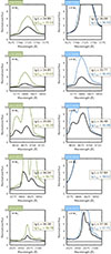 |
Fig. A.1. Optical emission lines predicted by our massive (Mini = 59 M⊙) and very massive (Mini = 131 M⊙), chemically homonegeously evolving, late-post-main-sequence models (classified as WO stars in this phase by Paper II; during the main-sequence evolutions, they were classified as early O type stars). In our fiducial population (Sect. 2.3), one or two such very massive stars are present with > 100 M⊙; in our alternative population (Sect. 3.1), about six such stars with ∼40 M⊙ and one with ∼80 M⊙ are present, accounting for the measured He II ionizing flux. For the explanation of the legends, see Fig. 6. Note that we always apply the unclumped models’ predictions (i.e. black line). |
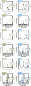 |
Fig. A.2. UV emission lines predicted by our models. See Fig. A.1. Note that we always apply the unclumped models’ predictions (i.e. black line), which is a conservative assumption. |
Appendix B: Ionizing flux predicted by our PoWR stellar atmosphere models
Number of ionizing photons predicted by our models in the Lyman, He I and He II continua, as well as the predicted hardness ratio I4686/IHβ = A⋅Q(He II)/Q(H I), explained in Sect. 3.2.
Appendix C: Stellar parameters of the new PoWR models computed for this work
Main parameters of the newly computed stellar atmosphere models, see Sect 2.2.
All Tables
Summary of the various measurements from the literature reproduced and discussed here.
Number of ionizing photons predicted by our models in the Lyman, He I and He II continua, as well as the predicted hardness ratio I4686/IHβ = A⋅Q(He II)/Q(H I), explained in Sect. 3.2.
Main parameters of the newly computed stellar atmosphere models, see Sect 2.2.
All Figures
|
Fig. 1. Left: Hertzsprung–Russell diagram summarizing the findings of Paper II (their Fig. 1 & Table 4) and our Sect. 2.2, showing that chemically homogeneous stellar evolution at I Zw 18 composition proceeds from class O via a shorter-lived class WN to a longer-lived WO phase – i.e. without experiencing any long-term WC phase. Evolutionary models are taken from Paper I (main-sequence) and Szécsi et al. (2022, post-main-sequence), without correcting for the wind optical depth (see the last paragraph of Sect. 2.2). Initial masses are labelled, showing where the tracks start their evolution, which proceeds towards the hot side of the diagram (i.e. CHE). Colours show the central helium mass fraction, and dots represent every 105 years of evolution. Dashes mark equiradial lines with 1, 10, and 100 R⊙ from left to right. The black star symbols represent the models for which PoWR synthetic spectra were computed in Paper II and Sect. 2.2. From right to left (note that the evolution progresses from red to blue, contrarily to classical massive-star evolution): main-sequence models with surface helium mass fractions of 0.28, 0.5, 0.75, and 0.98, while the fifth symbol on the very left corresponds to the core-helium-burning phase (post-main-sequence, Sect. 2.2). Spectral classification was performed in Paper II; the results (for four different assumptions about mass loss and clumping) were presented in their Table 4 and Appendix A. Here the labels summarize the ranges in class found there, except for the WN and WO stars which are discussed in Sect. 2.2 (see also Fig. 3). Right: HR diagram summarizing our findings from Paper I. Stellar models computed with I Zw 18’s chemical composition are shown following normal evolution (NE) towards the red supergiant branch with slow rotation (≲300 km s−1). With fast rotation, they are seen following CHE towards hot surface temperatures; that is, leftward from the ZAMS. This latter evolutionary path is what is elaborated upon in the left panel. For more details on how we construct a synthetic population out of both these kinds of models, see Sect 2.3. |
| In the text | |
|
Fig. 2. Spectral energy distributions of our PoWR synthetic spectra of chemically homogeneously evolving massive stars published in Paper II with the corresponding black body distributions overplotted for context. The models correspond to the second (MS) and last (pMS) phases on the HR diagram in Fig. 1; their main physical parameters and ionizing fluxes are listed in Table B.1. Titles indicate the initial mass of the evolutionary models with the actual mass (i.e. the mass when the synthetic spectra were computed) in parenthesis. The three main ionizing continua (Lyman: < 912 Å, He I: < 504 Å, He II: < 228 Å ) are marked (note the X scale showing the frequency instead of the wavelength, in order to spread out the relevant high-energy parts of the distributions). Framed boxes present the number of ionizing photons predicted by both the PoWR models (unclumped, with nominal mass-loss rates) and the black body distributions, in units of log(s−1); the values being close to each other is an interesting coincidence. Left column: Models in the main-sequence (MS) phase with surface helium mass fraction of YS = 0.5. Right column: Models in the post-main-sequence (pMS) phase (in the case of the 131 M⊙ model, the late-pMS phase, see Sect. 2.2 and Fig. 4). Note the order of magnitude difference in the Y scale between the left column and the right column. |
| In the text | |
|
Fig. 3. Time evolution of surface properties of the evolutionary model with Mini = 131 M⊙ after the terminal-age main sequence (TAMS). Reproduced from Szécsi (2016, their Fig. 4.13), adding information about our three post-main-sequence PoWR models scrutinized in Sect. 2.2 and Fig. 4. Black star-symbols mark their positions on the central helium mass fraction: YC = 0.8 (early), YC = 0.5 (mid), YC = 0.1 (late). The rudimentary classification of Szécsi (2016, see their Sect. 4.5.1, based on Georgy et al. 2012) is surpassed by the spectral-line-based classification scheme (see also Fig. 4 showing all the optical emission lines), meaning that chemically homogeneously evolving stars at I Zw 18 metallicity do not spend significant time in the WC phase, proceeding from their main-sequence O-star phase to WN and then directly to WO. |
| In the text | |
|
Fig. 4. PoWR model spectra of individual stars during the post-main-sequence (core-helium burning) phase of the same evolutionary model (Mini = 131 M⊙, actual mass between 93−106 M⊙). The model’s approximate position is shown on the HR diagram in Fig. 1 by the last point (pMS phase) at around log(Teff/K) ∼ 5.14 and log(L/L⊙) ∼ 6.7. Top: Optical range. Bottom: UV range. Nominal mass loss rate and no clumping was assumed, to be consistent with previous work (see Paper II, and the discussion of the caveats in Sect. 5.2). YC indicates core-helium abundance and thus the evolutionary progress during the post-MS. The earliest model (red straight line, YC = 0.8, i.e. just burned about 20% of its helium in the core) shows prominent emission only in helium, while the mid (blue straight line, YC = 0.5) and late (black straight line, YC = 0.1, corresponding to the bottom right panel of Fig. 2) ones develop carbon and oxygen lines too. (The Cl and S lines are modelling side-effects, we do not expect them to show up in observations.) However, the distinguishing emission line C IIIλ5696 Å which serves as the basis of classifying a stars as WC (Crowther et al. 1998) is missing in all three models. So are the nitrogen emission lines that would categorize a star as late-type WN (Crowther et al. 1995; Smith et al. 1996; Crowther & Walborn 2011). If observed, therefore, these stars would be identified as early-type WN (i.e. WN2) and then during most of the core-helium burning, as WO – more precisely, WO 2 evolving to WO 1. |
| In the text | |
|
Fig. 5. Top panel: Number of ionizing photons in the He II continuum in all our spectral models from Paper II. Evolutionary stages are indicated by colours (ZAMS by yellow; two main sequence models with surface helium mass fractions YS = 0.5 and 0.75 by green and red, respectively; terminal-age-main-sequence model, TAMS, by blue; and post-main-sequence model, pMS, by purple). For every evolutionary stage, QHe II from all four spectral models of Paper II are shown (hence the spread in the coloured stripes). Yellow circles represent the He II ionizing photon number computed from corresponding black body distributions (see Fig. 2). To account for a population of massive stars, we interpolate linearly between the logarithm of the three simulated masses. Models with nominal mass-loss rate and unclumped wind are used; interpolated values are shown with the solid black lines, small triangles marking the bin sizes. Above and below our highest and lowest mass models, the values of those models are applied (down to 9 M⊙). Bottom panel: Same as the top panel, but for the line luminosities in C IVλ1550 Å of the pMS model. The second trio of pink rectangles with higher values correspond to clumped wind models (see also Fig. 6). Other line luminosities are treated the same way (see Sect. 2.4). |
| In the text | |
|
Fig. 6. Normalized flux around the UV line C IVλ1550 Å in three post-main-sequence (l-pMS) spectral models with initial masses as indicated in the top left corner of the panels. Line luminosity (computed following Sect. 2.4) is given in the framed boxes in units of log(erg s−1); lg L stands for unclumped (clumping factor D = 1) while lg Lcl for clumped (D = 10) wind, see details in Paper II. When creating the synthetic population here (Sect. 2.3 and Sect. 3.1), we always apply the unclumped models’ predictions (i.e. black line). Other emission lines are presented in Figs. A.1–A.2. Based on this, we predict a ∼40–50 Å-wide emission bump from our population between 1550–1600 Å, which is indeed present in the observations in Fig. 11. |
| In the text | |
|
Fig. 7. Hertzsprung–Russell diagrams with background colours representing the number of Lyman (left) and He-II (right) continuum photons emitted by a black body with a given temperature and luminosity. Units are associated with colours (pink: 1048 ph s−1, blue: 1049 ph s−1, green: 1050 ph s−1, #FAF2BF;: 1051 ph s−1; a black background means < 1048 ph s−1). Stellar evolutionary model sequences are labelled with their initial masses. They are taken from the BoOST project (Szécsi et al. 2022), except for the turquoise line, which is a stripped binary model from Götberg et al. (2017). White lines mean Milky Way composition, where all models evolve the ‘normal’ way (although the most massive ones turn to the left eventually: this is classical Wolf–Rayet evolution). Purple and golden lines mean I Zw 18 composition, with one of the very massive models evolving normally (initial rotational velocity of 100 km s−1) and the others chemically homogeneously due to fast rotation (500 km s−1). Every 105 yr of evolution is marked with dot on the tracks. Including the 20 M⊙ model into our population synthesis runs (with a sufficiently long star formation episode, see Table 1) hardens the combined spectra considerably (reaching close to the observed I(4686)/I(β) ∼ 0.02), as the late phases of this model enter the pink zone in terms of He-II photons while not leaving the blue zone in terms of Lyman photons. For more details on the population synthesis and spectral hardness, see Sects. 2.3 and 3.2, respectively. |
| In the text | |
|
Fig. 8. Optical spectra reproduced from Izotov et al. (1997, their Fig. 1). Spectrophotometric observations were obtained by the MMT Observatory using a 1 |
| In the text | |
|
Fig. 9. Optical spectra reproduced from Thuan & Izotov (2005, their Fig. 2). Observation taken with the MMT spectrograph (blue channel) at the 6.5 m MMTO. A 2″ × 300″ slit was used, and the brightest part of the north-western H II region was extracted using a 6″ × 2″ extraction aperture. For our discussion, see Sect. 4.1. |
| In the text | |
|
Fig. 10. Optical spectra reproduced from Kehrig et al. (2016, their Figs. 2 & 6, here top & middle, respectively) and Kehrig et al. (2015a, their Fig. 3, bottom). Integral field spectroscopy was obtained with the Potsdam Multi-Aperture Spectrophotometer (PMAS) on the 3.5 m telescope at the Calar Alto Observatory (Almeria, Spain). Top: Hβ map with a cross marking where the spectrum in the middle was extracted from. Middle: Spectrum showing a prominent WR-bump associated with stellar emission underneath the narrow, nebular He IIλ4686 Å line, discussed in Sect. 4.1. Bottom: Integrated spectrum of the north-western region of I Zw 18, demonstrating how stellar emission bumps clear out completely when the full galaxy is integrated over, leaving only the narrow nebular component. Compare this to the FUSE data in Fig. 12, which we discuss in Sect. 4.2. |
| In the text | |
|
Fig. 11. UV spectra reproduced from Brown et al. (2002, their Fig. 1). Observations taken with Hubble’s Space Telescope Imaging Spectrograph (STIS) using the G140L grating and the 52″ × 0 |
| In the text | |
|
Fig. 12. UV spectra reproduced from Lecavelier des Etangs et al. (2004, their Fig. 1). Observation taken with FUSE, with an aperture (30″ × 20″) covering the whole galaxy. Top: Position of the observation; picture is taken from the MAST archives with background image from Pan-STARRS. Bottom: Spectra presented in Lecavelier des Etangs et al. (2004). Since the full galaxy is in the aperture, the features of the localized stellar populations are not expected to be seen (see Fig. 10, as well as our discussion in Sect. 4.2). |
| In the text | |
|
Fig. 13. UV spectra reproduced from Heap et al. (2015, their Fig. 5). Top: Regions of the Hubble COS observations according to the MAST archive (PI: J.C. Grean, year: 2010, aperture: 2 |
| In the text | |
|
Fig. 14. HST measurements of I Zw 18. The panel labelled MAST/Pan-STARRS shows the circular aperture used for obtaining the highest signal-to-noise-ratio UV spectrum of I Zw 18 available to date, taken by COS (Berg et al. 2022). Circle and background image are the same as in Fig. 13 (taken from the MAST archive applying background image from the Pan-STARRS survey). The panels to the left correspond to STIS copied from Brown et al. (2002, mentioned also in Sect. 4.2 and Fig. 11, see details there). The positions where Brown et al. (2002) identified WR-like emission bumps (c and d) are marked by Xs for convenience. The panel labelled MAST/DSS demonstrates a discrepancy we found in the MAST Archive’s AstroView tool (see Sect. 4.3 for details). Our explanation for why the COS spectrum analysed by Berg et al. (2022, see their Fig. 12) does not display C IV emission – despite at least one of the Brown-sources seemingly being within the aperture – is that the field of view includes too much contaminating light: as demonstrated by Kehrig et al. (2016) using integral field spectroscopy of I Zw 18 (see our Fig. 10), stellar emission bumps clear out completely unless the spectra is taken from the right physical position of the galaxy. |
| In the text | |
|
Fig. A.1. Optical emission lines predicted by our massive (Mini = 59 M⊙) and very massive (Mini = 131 M⊙), chemically homonegeously evolving, late-post-main-sequence models (classified as WO stars in this phase by Paper II; during the main-sequence evolutions, they were classified as early O type stars). In our fiducial population (Sect. 2.3), one or two such very massive stars are present with > 100 M⊙; in our alternative population (Sect. 3.1), about six such stars with ∼40 M⊙ and one with ∼80 M⊙ are present, accounting for the measured He II ionizing flux. For the explanation of the legends, see Fig. 6. Note that we always apply the unclumped models’ predictions (i.e. black line). |
| In the text | |
|
Fig. A.2. UV emission lines predicted by our models. See Fig. A.1. Note that we always apply the unclumped models’ predictions (i.e. black line), which is a conservative assumption. |
| In the text | |
Current usage metrics show cumulative count of Article Views (full-text article views including HTML views, PDF and ePub downloads, according to the available data) and Abstracts Views on Vision4Press platform.
Data correspond to usage on the plateform after 2015. The current usage metrics is available 48-96 hours after online publication and is updated daily on week days.
Initial download of the metrics may take a while.