| Issue |
A&A
Volume 703, November 2025
|
|
|---|---|---|
| Article Number | A104 | |
| Number of page(s) | 29 | |
| Section | Galactic structure, stellar clusters and populations | |
| DOI | https://doi.org/10.1051/0004-6361/202554112 | |
| Published online | 14 November 2025 | |
The GALAH survey: Improving chemical abundances using star clusters
1
Faculty of mathematics and physics, University of Ljubljana,
Jadranska 19,
1000
Ljubljana,
Slovenia
2
Research School of Astronomy and Astrophysics, Australian National University,
Canberra,
ACT 2611,
Australia
3
ARC Centre of Excellence for All Sky Astrophysics in 3 Dimensions (ASTRO 3D),
Australia
4
ACCESS-NRI, Australian National University,
Canberra,
ACT2601,
Australia
5
Sydney Institute for Astronomy, School of Physics, A28, The University of Sydney,
NSW 2006,
Australia
6
Australian Astronomical Optics, Faculty of Science and Engineering, Macquarie University,
Macquarie Park,
NSW 2113,
Australia
7
Department of Physics, University of Rome Tor Vergata,
via della ricerca scientifica 1,
00133,
Rome,
Italy
8
Homer L. Dodge Department of Physics & Astronomy, University of Oklahoma,
440 W. Brooks St.,
Norman,
OK
73019,
USA
9
School of Physics, University of New South Wales,
Sydney,
NSW 2052,
Australia
10
Department of Astronomy, Stockholm University, AlbaNova University Centre,
106 91
Stockholm,
Sweden
11
Space Telescope Science Institute,
3700 San Martin Drive,
Baltimore,
MD,
21218,
USA
12
School of Mathematical and Physical Sciences, Macquarie University,
Balaclava Road,
Sydney,
NSW 2109,
Australia
13
Astrophysics and Space Technologies Research Centre, Macquarie University,
Balaclava Road,
Sydney,
NSW 2109,
Australia
14
International Space Science Institute Beijing,
1 Nanertiao, Zhongguancun,
Beijing
100190,
China
15
School of Physics and Astronomy, Monash University,
Clayton,
VIC 3800,
Australia
16
Theoretical Astrophysics, Department of Physics and Astronomy, Uppsala University,
Box 516,
751 20
Uppsala,
Sweden
17
Stellar Astrophysics Centre, Aarhus University,
Ny Munkegade 120,
8000
Aarhus C,
Denmark
★ Corresponding author: This email address is being protected from spambots. You need JavaScript enabled to view it.
Received:
12
February
2025
Accepted:
16
August
2025
Abstract
Large spectroscopic surveys aim to consistently compute stellar parameters of very diverse stars, while minimizing systematic errors. We explore the use of stellar clusters as benchmarks to verify the precision of spectroscopic parameters in the fourth data release (DR4) of the GALAH survey. We examine 58 open and globular clusters and associations to validate measurements of temperature, gravity, chemical abundances, and stellar ages. We focus on identifying systematic errors and understanding trends between stellar parameters, particularly temperature and chemical abundances. We identify trends by stacking measurements of chemical abundances against effective temperature and modelling them with splines. We also re-fit spectra in three clusters with the Spectroscopy Made Easy and Korg packages to reproduce the trends in DR4 and to search for their origin by varying temperature and gravity priors, linelists, and the spectral continuum. Trends are consistent between clusters of different ages and metallicities, can reach amplitudes of ~0.5 dex, and differ for dwarfs and giants. We use the derived trends to correct the DR4 abundances of 24 and 31 chemical elements for dwarfs and giants, respectively, and publish a detrended catalogue. While the origin of the trends could not be pinpointed, we found that: (i) photometric priors affect derived abundances, (ii) temperature, metallicity, and continuum levels are degenerate in spectral fitting, and it is hard to break the degeneracy even by using independent measurements, (iii) the completeness of the linelist used in spectral synthesis is essential for cool stars, and (iv) different spectral fitting codes produce significantly different iron abundances for stars of all temperatures. We conclude that clusters can be used to characterise the systematic errors of parameters produced in large surveys, but further research is needed to explain the origin of the trends.
Key words: methods: data analysis / techniques: spectroscopic / surveys / stars: abundances / globular clusters: general / open clusters and associations: general
© The Authors 2025
 Open Access article, published by EDP Sciences, under the terms of the Creative Commons Attribution License (https://creativecommons.org/licenses/by/4.0), which permits unrestricted use, distribution, and reproduction in any medium, provided the original work is properly cited.
This article is published in open access under the Subscribe to Open model. This email address is being protected from spambots. You need JavaScript enabled to view it. to support open access publication.
1 Introduction
Large spectroscopic surveys of stars observe hundreds of thousands or even millions of stars, and these numbers are expected to increase significantly in the coming years with the commissioning of new, highly multiplexed instruments such as WEAVE (Jin et al. 2024) and 4MOST (de Jong et al. 2019). The scientific goals of these surveys encompass a wide range of topics in stellar physics and Galactic science, necessitating observations of a diverse population of stars found throughout the Galaxy and beyond.
It is the job of the analysis pipelines to derive stellar parameters from diverse spectra consistently and homogeneously (Jofré et al. 2019). Parameters for different stellar types and spectral qualities must be comparable with minimal systematic uncertainties. The performance of these pipelines is typically monitored using a set of benchmark stars âĂŤ- stars that have high-quality, well-studied spectra and whose parameters are measured independently through various methods (e.g. Heiter et al. 2015; JofrÃl’ et al. 2018; Adibekyan et al. 2020). Typically, a relatively small number of benchmark stars are observed with each instrument to assess the accuracy of the instruments and the analysis process, as well as to determine the zero points for certain parameters and to homogenise them across different surveys or instruments when needed. However, benchmark stars can rarely measure the precision of derived parameters, which would require a statistically large sample of benchmark stars that are representative of the whole survey. Additionally, benchmark stars are not suitable for probing the influence of atmospheric models, linelists, and algorithms in spectral fitting codes if both benchmark stars and science targets are analyzed using the same analysis approach. While spectral fitting codes (such as SME (Valenti & Piskunov 1996; Piskunov & Valenti 2017) and Turbospectrum (Plez 2012; Gerber et al. 2023)), atmospheric models (e.g. Gustafsson et al. 2008; Magic et al. 2013) and linelists (Smith et al. 2021; Heiter et al. 2021) have been well tested, any issues affecting both benchmark stars and science stars alike might go undetected or, worse, misinterpreted as genuine physical phenomena.
In this work, we explore the use of open clusters, young associations, and some globular clusters as benchmarks to derive more precise stellar parameters, specifically focusing on the abundances of chemical elements. Star clusters as benchmarking objects are complementary to the benchmark stars. Stars in clusters, particularly in open clusters, are resolved conatal, coeval populations for which we can assume high level of chemical homogeneity (Krumholz et al. 2019; Kos et al. 2021). We can test whether the spectral fitting codes indeed produce consistent values of abundances of chemical elements across a large range of temperatures and stellar types. This approach is particularly beneficial, as we can often observe more stars in a single cluster than the total number of benchmark stars available in the entire survey. We can independently test the consistency of measured abundances across various stellar types and temperature ranges, which is not feasible for benchmark stars. Because open clusters are chemically homogeneous (Bovy 2016; Poovelil et al. 2020; Sinha et al. 2024), they are best suited for our analysis. Many globular clusters, however, contain multiple stellar populations (Milone & Marino 2022; Gratton et al. 2019), and thus we cannot assume that they are chemically homogeneous. They can still be used to search for trends in the analysis, if those trends are consistent across multiple populations or if they are larger than the chemical inhomogeneities. Stars in very young clusters or associations can also show chemical patterns that resemble systematic trends; for example, due to fast rotation, strong magnetic fields or pre-main-sequence evolution (Spina et al. 2020). Even for open clusters, we cannot assume that stars of all types will show chemical homogeneity for all elements due to atomic diffusion (Dotter et al. 2017; Moedas et al. 2022), convective motion (Grassitelli et al. 2015), or dredge-up effects (Smith & Lambert 1990; Loaiza-Tacuri et al. 2023). Hence, we only analyse systematic trends that are consistent in clusters in a large age and metallicity range and we take caution for elements such as Li, C, N, and O.
Using the observations of clusters, we evaluate the precision1 of the recent fourth data release (DR4) of the GALAH survey (Buder et al. 2024). It provides measurements of abundances of up to 32 elements from spectra of 917 588 stars. The main goal of the survey is to measure the abundances of chemical elements in a wide range of Galactic stars to support studies in the fields of stellar physics and galactic archaeology (De Silva et al. 2015; Martell et al. 2017). In DR4, we observe trends – systematic patterns – when plotting the abundances of chemical elements against effective temperature. Similar trends were observed recently in other surveys using visible and near-infrared spectra, and in spectra with low and high resolution (Casali et al. 2020; Fu et al. 2022; Magrini et al. 2023; Grilo et al. 2024; Reyes et al. 2024). Non-physical discrepancies between the abundances measured in giants and dwarfs were observed as well (Dutra-Ferreira et al. 2016; Dal Ponte et al. 2024). This study aims to characterise these trends, assess their consistency, and explore potential empirical origins. We also publish a detrended catalogue of abundances of chemical elements.
In addition to examining the precision and systematic errors in the measurements of chemical element abundances, we investigate the discrepancies in effective temperatures, surface gravities, and ages of stars as reported in DR4. In clusters, these can be measured very precisely, due to high-quality photometric and astrometric observations of almost all GALAH stars, and because coeval cluster stars must lie on the same isochrone, which can be accurately determined from a large number of stars in a cluster (see previous work based on GALAH DR4 in Beeson et al. 2024). The systematic discrepancies between temperatures, gravities, and ages determined from isochrones compared to those from spectra may originate from similar sources as the trends observed in the measurements of chemical abundances – which is the hypothesis explored in this work. While we present several issues regarding the parameters in GALAH DR4, it is important to note that significant improvements have been made since the third data release in terms of data reduction and analysis. This has resulted in improved precision, accuracy, and new parameters reported in DR4.
This paper is structured as follows. Section 2 presents the spectroscopic parameters from GALAH DR4 and clusters that are used in this work. In Section 3, we derive the trends in the measurements of the abundances of chemical elements and explore their potential origins in Section 4. Then, we dedicate two sections to the verification of stellar ages reported in GALAH DR4 (Section 5) and temperature and surface gravity (Section 6). The paper concludes with some discussions and implications of this study in Section 7. Functional forms of the derived trends and instructions on how to use them are given in the appendix.
2 Data
In this work we combine the spectroscopic observations and parameters obtained in the GALAH survey with parameters of open clusters, young associations, and globular clusters sourced from the literature.
2.1 Spectroscopic data and GALAH DR4
GALAH DR4 is the latest by the GALAH collaboration. Stars are observed with the 3.9 m AAT telescope at the Siding Spring Observatory in Australia with the 2 dF instrument (Lewis et al. 2002). Around 350 targets we observe simultaneously, with spectra obtained with the HERMES spectrograph (Sheinis et al. 2015). The spectrograph consists of four arms, producing spectra in roughly 250 Å wide bands in blue, green, red, and infra-red channels. The wavelength ranges of the channels were selected such that they cover prominent absorption lines of as many chemical elements as possible. Hydrogen’s Hα and Hβ Balmer lines are also included, as well as several interstellar lines (KI doublet and some strong diffuse interstellar bands). The same set-up is used by several observing programmes, the largest being the main GALAH survey, which we complement with dedicated observing programmes of clusters, young associations, and K2 targets, turn-off stars, bright fields observed during twilight, and some public data produced by third party observers throughout the last ten years of operations. Public data were only used if the observers did not deviate from the observing procedures required by the GALAH survey (choice of calibration fields, targeting constraints, magnitude limits etc., see Buder et al. (2024)). All these observations are combined in GALAH DR4. They are reduced with a common pipeline dedicated to the requirements of the GALAH survey (Kos et al. 2017; Buder et al. 2021, 2024). The pipeline produces reduced and normalised spectra, and calculates the first estimates for stellar radial velocities and basic spectroscopic parameters (temperature, gravity, metallicity, rotational broadening, and microturbulence velocity). The pipeline also produces a resolution profile for each observed spectrum.
The reduced data are processed by an analysis pipeline. The main component of the pipeline is the fitting of observed spectra with synthetic spectra. The difference is minimised between an observed and synthesised spectrum with some labels, which represent the parameters we are trying to fit. The labels (including abundances of 31 chemical elements) are fitted across the whole wavelength range simultaneously. To make this computationally feasible, synthetic spectra are produced only on a grid of discrete Teff, log g, and [Fe/H] using SPECTROSCOPY MADE EASY (SME) (Valenti & Piskunov 1996; Piskunov & Valenti 2017), MARCS atmosphere models (Gustafsson et al. 2008), a linelist adapted from Heiter et al. (2021), Grevesse et al. (2007) solar abundances, and non-local-thermodynamicequilibrium (non-LTE) departure coefficients for elements H, Li, C, N, O, Na, Mg, Al, Si, K, Ca, Mn, and Ba (Amarsi et al. 2020). A neural network similar to THE PAYNE (Ting et al. 2019) is then used to interpolate spectra from a grid to any (physically sensible) set of labels. With this approach, a synthetic spectrum can be produced in a fraction of a second, which enables a quick global fitting process. On-the-fly continuum normalisation and resolution matching is done while fitting.
First, the individual observations are analysed, which produces an initial set of labels (dataset with allspec in the name of GALAH DR4 products). Radial velocities are inspected, and observations of different epochs are then combined into a single spectrum. SB2 binaries are flagged, and SB1 binaries have spectra shifted based on their measured radial velocities. Combined spectra are re-analysed, this time also by including photometric information to constrain log g and help resolve degeneracies when fitting many labels at once. Labels derived for combined spectra (dataset with allstar in the name of GALAH DR4 products) are the ones we use in this work. This means that we use only one set of labels for each star, regardless of the number of repeated observations. Any subsequent quality cuts used in this work are described further in the text.
2.2 Open cluster data
We use Cantat-Gaudin et al. (2020) as a primary source of stars in open clusters, which we append with Hunt & Reffert (2024). We find both catalogues to be very reliable and sufficiently extensive; however, for some clusters one catalogue includes members that the other does not. We made a cross match between these catalogues and GALAH DR4 stars to obtain a list of 3353 stars in 93 open clusters. Most clusters contain only a small number of stars observed in the GALAH survey. These were observed serendipitously throughout the survey. A small fraction of the clusters were observed intentionally, and they contain a larger number of observations. Here we only consider clusters with five or more observed stars. A list of open clusters used in this work is given in Table A.1.
2.3 Globular cluster data
Here we use the same selection of globular cluster stars as in the main DR4 paper (Buder et al. 2024). Stars were searched for in a six-dimensional parameter space (sky positions, distances, and proper motions obtained from Gaia DR3, and radial velocity from GALAH DR4) around the positions of known globular clusters sourced from Vasiliev & Baumgardt (2021). Stars in 28 globular clusters were identified. The summary of globular clusters with more than ten observed stars, used in this work, is listed in Table A.2. For the purpose of this work, we use globular cluster ages from Marín-Franch et al. (2009) (Table 4, column G00CG) and from Cabrera-Ziri & Conroy (2022). Typical uncertainties are 0.6 Gyr. We also use metallicities from Schiavon et al. (2024); Massari et al. (2017); O’Malley & Chaboyer (2018); Monaco et al. (2018); Muñoz et al. (2021).
2.4 Young association data
We treat stars in young associations separately from open clusters, although some stars in young associations are assembled into clusters included as part of open clusters in Table A.1. Many stars in young associations are not bound into dense clusters, as they have dispersed significantly since their birth. They can still be identified as members of the association, which can also be partitioned into smaller building blocks (e.g. Zari et al. 2018; Chen et al. 2020; Ratzenböck et al. 2023). These, however, do not necessarily satisfy the conditions for being open clusters, and are thus not properly surveyed in open cluster catalogues. We make no distinction between open clusters and associations, apart from using additional catalogues to cross-match stars in young associations. Our main focus is on the elemental abundances and ages of the stars, and if we can confirm the common origin of stars, it is irrelevant whether they are part of a gravitationally bound cluster or a dispersing association.
GALAH observed numerous stars in three nearby young associations (Orion OB1, Vela OB2, and the Scorpius-Centaurus-Crux). We used third party catalogues, which we cross-matched with GALAH observations to identify stars in the associations. The selected catalogues were also required to provide subdivisions of the association stars into smaller groups. These have to form meaningful groups based on their kinematics and ages, and at the same time be large enough for the GALAH survey to be able to observe a statistically relevant number of stars in a group (we aimed for groups with at least 20 stars observed in GALAH). If a hierarchical structure of an association is provided in the literature (Larson 1981; Vázquez-Semadeni et al. 2017; Sun et al. 2018; Ratzenböck et al. 2023), we did not necessary partition an association into the smallest possible groups to avoid the undersampling described above. The summary of the associations and their subdivisions used in this work is given in Table A.3. For the names of subdivisions, we use the same names as the original papers.
2.4.1 Vela
We used Cantat-Gaudin et al. (2019) to select stars in the Vela OB2 association and its sub-groups. All regions in Vela were observed serendipitously, except for population 7 (including cluster γ2 Vel) and population 4 (including Collinder 135 and 140, and NGC 2451B).
2.4.2 Orion
For the Orion OB1 association and the λ Orionis group, we use regions defined in Kos et al. (2019, 2021). For the purpose of this work, we use subdivisions known as the λ Orionis group, Orion OB1a, OB1b, a single region including Orion OB1c and OB1d, and the region of the NGC 1788 cluster. All stars in Orion were targeted intentionally.
2.4.3 Scorpius-Centaurus-Crux
Clustering for the Scorpius-Centaurus-Crux region was taken from Žerjal et al. (2023). Some regions in Sco-Cen-Cru were observed intentionally within different observing programmes. Some regions were observed serendipitously; hence, there is a large difference between the number of stars observed in each region.
3 Deriving trends in the abundances of chemical elements
Any deviation from chemical homogeneity within a cluster should be of a physical nature, meaning that the measured abundances of chemical elements should be identical for all stars within a cluster, regardless of factors such as the quality of the spectra, observing time, resolution, or the observed wavelength bands. Any deviations from this expectation should be of a physical nature. However, a quick examination of the abundance measurements across clusters reveals that this is not the case in practice; various factors are likely causing systematic deviations or trends. In this section, we demonstrate that many of these trends are consistent across different clusters and provide a way to parametrise them.
When initially exploring the trends, we considered the trends of abundances as a function of several stellar and spectroscopic parameters (temperature, gravity, projected rotational velocity, microturbulence velocity and the signal-to-noise ratio of the spectra). We realised that the trends were most coherent when displayed as a function of temperature. In addition, when deriving the trends with temperature and de-trending the elemental abundances, we found no significant residual trends with other parameters. We conclude that any trends initially observed with other parameters must have existed due to the correlations of those parameters and temperature. Hence, in the rest of this work we only present trends as a function of stellar effective temperature.
The aim is to calculate trends for as many elements as possible and for the largest possible range of temperatures. We separate the trends based on the spectral type of the stars (giants and dwarfs, where the distinction between them is described in the next section) and further dissect them for the trends valid for unflagged stars only and all stars (both flagged and unflagged stars). GALAH DR4 provides two main sets of flags that indicate issues with the given data products. A flag_sp value indicates issues with a star or its spectra. In this work we consider all stars with flag_sp < 8 as unflagged stars. This means we ignore flags indicating a detected emission in Hα or Hβ, flags indicating spectra where one of the four channels is missing (the IR channel is missing for a small number of observations), and flags marking the SB1 binaries. All other issues indicated by flag_sp are considered as valid flags in this work. Additionally, a flag_x_fe (x being an element) indicates issues with the measurements of the abundance of one particular element. If this flag is raised, we consider the measurements for that element as flagged.
3.1 Distinction between giants and dwarfs
Our initial inspection of the trends showed that they can be different for giants and dwarfs. This can be expected for different reasons, including differences in model atmospheres used in spectral synthesis, different linelists, sensitivity to the isochrone fitting and photometric priors (see Beeson et al. 2024), or the correlation between the temperature and signal-to-noise ratio per pixel (S/N, in general, is correlated for dwarfs and anticorrelated for giants Buder et al. 2021, Figure 3, right). Hence, we split the stars into giants, dwarfs, and a small region around the turn-off (subgiants), which we call the overlap region. The overlap is necessary to verify the trends for giants and dwarfs in the region where one trend should smoothly transition into the other. It is possible that giants and dwarfs experience completely different trends with no smooth transition. However, for the purpose of detrending the data, a smooth transition is preferred.
The distinction between dwarfs and giants was done in the Kiel diagram. We chose two regions: one defining the giants and one defining the overlap. Stars outside these two regions are considered to be dwarfs. The regions are defined (arbitrary) as
![Mathematical equation: $\[\begin{cases} & \text {if} ~T_{\text {eff }}<6300 \mathrm{~K} \text { and } \\ \text { giants, } & \log~ g<\left(-0.000158 ~T_{\text {eff }} / \mathrm{K}-5670\right)+3.8 \text { and } \\ & \log~ g<\left(0.000459 ~T_{\text {eff }} / \mathrm{K}-5670\right)+4.2 \text { and } \\ & \log~ g<\left(0.002 ~T_{\text {eff }} / \mathrm{K}-4800\right)+3.8. \\\\ & \text {if} ~T_{\text {eff }}<6300 \mathrm{~K} \text { and } \\ \text { overlap, } & \log~ g<\left(-0.000158 ~T_{\text {eff }} / \mathrm{K}-5670\right)+4.2 \text { and } \\ & \log~ g<\left(0.000459 ~T_{\text {eff }} / \mathrm{K}-5670\right)+4.2 \text { and } \\ & \log~ g \geq\left(-0.000158 ~T_{\text {eff }} / \mathrm{K}-5670\right)+3.8. \\\\ \text { dwarfs, } & \text {otherwise.}\end{cases}\]$](/articles/aa/full_html/2025/11/aa54112-25/aa54112-25-eq2.png) (1)
(1)
Figure 1 shows the Kiel diagram with all stars used to determine the trends in this work. Regions defining dwarfs, giants. and the overlap are marked as well.
The only exception to this classification are globular clusters where we observed a small number of stars on the horizontal branch. The distribution of the horizontal branch stars stretches into the dwarfs region, as defined above. Therefore, we designated all stars in globular clusters as giants. There are no dwarfs observed in any globular cluster in the GALAH survey.
3.2 Parametrising the trends
After the initial inspection of the trends, we had decided to parameterise the trends with cubic splines. The goal is to describe smooth trends at higher temperatures and a sharp transition at lower temperatures with a single function. After initial experimentation, any polynomials were ruled out, because very large orders would be needed to describe the aforementioned features. For some elements and for some clusters we did not have enough data points to reliably fit the trends with high-order polynomials. We used cubic splines instead.
A univariate cubic spline is a piecewise function of the form
![Mathematical equation: $\[f_i(x)=A ~x^3+B ~x^2+C ~x+D,\]$](/articles/aa/full_html/2025/11/aa54112-25/aa54112-25-eq3.png) (2)
(2)
where i are sections of the function between consecutive knots. In the knots, the following conditions of continuity up to the second derivative must be satisfied:
![Mathematical equation: $\[\begin{aligned}f_i\left(x_i\right) & =f_{i+1}\left(x_i\right), \\f_i^{\prime}\left(x_i\right) & =f_{i+1}^{\prime}\left(x_i\right), \text { and } \\f_i^{\prime \prime}\left(x_i\right) & =f_{i+1}^{\prime \prime}\left(x_i\right),\end{aligned}\]$](/articles/aa/full_html/2025/11/aa54112-25/aa54112-25-eq4.png) (3)
(3)
where xi is the position of a knot. We selected the positions of the knots, so they separate different regimes of the trends. We fixed the knots at 3800, 4200, 4750, and 5700 K. A cubic spline was fitted to the trends by a chi-square minimisation method. In practice, both the definition of the spline function and the fitting procedure were handled by the scipy’s LSQUnivariateSpline function (Virtanen et al. 2020). Additionally, we skipped a knot xi, if the function fi+1 was to be constrained by just five or fewer data points.
Instead of coefficients A to D for each segment, scipy produces coefficients of B-spline base functions. How the fitted function can be generated from coefficients, positions of knots, and the order of the spline is explained in Appendix C.
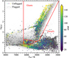 |
Fig. 1 Kiel diagram of the stars used to compute the trends. Unflagged stars are plotted with colours and flagged stars with grey crosses. The grey background distribution shoes all stars in GALAH DR4. Regions delineating dwarfs, giants, and the overlap region are marked in red. The equations of all red lines are specified in Equation (1). |
3.3 Stacking trends of individual clusters
We wish to define trends that are uniformly valid over as large parts of the temperature range as possible. This is hardly feasible by using observations in a single cluster, as only stars in a narrow range of temperatures are usually observed. Hence, we combine observations of multiple clusters, so we can fit a single trend representative of all clusters. Because stars in clusters have different compositions, one should not fit trends onto the joined measurements of abundance vs. effective temperature. Instead, we first fit a trend to the measurements of each individual cluster, and then join measurements from individual clusters by shifting them accordingly. This way we can later fit the trends onto joint data-sets with minimal scatter. We determined the required shift independently for each cluster and for each chemical element. We shifted the data by the value of the trend at Teff = 5400 K for the dwarfs and at Teff = 4800 K for the giants. We wanted to select the value for the dwarfs close to the temperature of the Sun, where we believe the abundances are the most accurate. However, a lot of clusters do not have any stars observed at the temperature of the Sun. Instead we chose a temperature of Teff = 5400 K where we have observations for most clusters; therefore, we do not have to extrapolate the trend just to determine the required shift. For giants we selected the temperature close to the red clump, where GALAH abundances should be most accurate. If the extrapolation of the trend beyond the extent of the data is still needed, we assume a constant value at the edge of the data range. Note that the selection of the temperature where we believe the abundances are most accurate is arbitrary. If chosen poorly, detrending can reduce accuracy (but improve precision in either case). We believe that the chosen values are adequate and the accuracy of individual measurements is indeed improved. However, we use precision to evaluate the improvement detrending makes to populations of stars or the survey as a whole.
Figure 2 illustrates the trends for a small (morphologically representative) number of elements observed in seven open clusters of different ages (top panel, showing the trends for dwarfs) and seven clusters with different metallicities (bottom panel, showing the trends for giants). Note that the trends observed in unrelated clusters display a similar shape. This led us to believe that the trends are not peculiar but rather general, i.e. they are not caused by the properties of clusters (such as an abundance of active stars in young clusters, fast rotators etc.) or data reduction (such as correlation between the S/N and temperature on the main sequence, continuum fitting, etc.). Some features, such as the steep trend in the iron abundance of the coldest stars, are common to both dwarfs and giants.
3.4 Fitted trends
We fitted the trends separately for dwarfs and giants, with the stars from the overlap region being included in both domains. For some elements the uncertainties in their abundance measurement were too large to fit meaningful trends.
For all elements, for dwarfs and giants, the trends were fitted with cubic splines, with the same algorithm as for individual clusters in the previous two sections. The S/N of each star measured in the red channel was used as a weight in the fitting algorithm. Additionally, we found the fit to perform best with an arbitrary increase in the weights of unflagged stars by a factor of 3. The first reason for giving unflagged stars a higher weight is that we trust unflagged measurements more. The second reason is that we want to use a single function for detrending. Using a different function for flagged and unflagged stars would produce discontinuities in the final table of abundances. We can avoid this by making the function for flagged stars follow the function for unflagged very tightly in the overlapping temperature range. Figures D.1 and D.2 show the fitted trends for all elements.
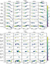 |
Fig. 2 Trends for several clusters illustrated for a small selection of elements. Top: Trends for seven open clusters and associations. The last row shows the combined measurements. Bottom: Trends for eight open and globular clusters. Quantities in the first column are shifted by the value of [Fe/H] given under the cluster’s name, so they fit into the same plotting range. The coloured points are unflagged stars; grey crosses are flagged stars. The solid line is a fit for unflagged stars; the dashed line is a fit for all stars. Trends fitted to the complete dataset of clusters are different from those in this illustration and are explained in Section 3.4 and Appendix B. |
3.5 Detrending
A product of this work is a table of abundances of chemical elements as measured in GALAH DR4, but detrended with the relations calculated here. The other parameters given in Tables B.1 and B.2 were not modified.
For detrending we used the trends derived from the combined fit of flagged and unflagged stars. Consequently, the trends are constrained only by observations of flagged stars in some temperature regions. This is not ideal, but allows us to detrend measurements for valuable stars that might have temperatures outside the temperature ranges of our unflagged cluster stars. One can also notice from Figures D.1 and D.2 that such a generalisation is justified, as the trends derived with the inclusion of flagged stars are usually a good extrapolation of the trends derived from unflagged stars only.
GALAH stars (regardless of their S/N or flags values) were first split into dwarfs, giants, and stars from the overlap, as defined in Section 3.1. Elements that need to be detrended were selected. For dwarfs we only detrended the measurements of the abundances of [Fe/H] and [X/Fe] for elements X (O, Na, Mg, Al, Si, K, Ca, Sc, Ti, V, Cr, Mn, Co, Ni, Cu, Zn, Rb, Sr, Y, Zr, Ba, Nd, and Sm). For giants we also included elements C, N, Mo, Tu, La, Ce and Eu. Other elements show trends that are much smaller than the scatter of the abundance measurements in our cluster stars, or only have abundances measured in such small numbers of stars that the trends cannot be reliably calculated. Next, we calculated the correction (value of the derived trend at some temperature) for each measurement, if the temperature of the star lies within the boundaries where the trend is defined. The value of the correction was subtracted from the original measurement to produce a detrended measurement. For the stars in the overlap region between dwarfs and giants, we subtracted the mean of both trends. Whether the stars lie in the dwarfs or giants region was determined based solely on the DR4 Teff and log g.
The schema for a table of detrended abundances is the same as the one for the allstars table in GALAH DR4 (see schema in Table 7 of Buder et al. 2024) with the following modifications. Every measurement that was not detrended (either for a particular star or the element as a whole) has an additional flag in the flag_X_Fe column of the stellar parameters table. The flag was increased by a value of 128 (8th bit was raised in the flag value). An additional column (detrend_model) was added. The value in this column is set to 0, if trends for dwarfs were used to detrend the measurements for a star, 1, if trends for giants were used, and 2, if a star belongs to the overlap region, so a combination of trends for giants and dwarfs was used. When using the detrended table, one can treat the flags similarly as in the original table; small flag values mean reliable data, while large flag values indicate caution or poor data.
4 Origin of the trends
In this section we discuss some possible causes for the trends observed in the relation between abundances of chemical elements and stellar effective temperature. We try to explain two general features observed for many elements. First, is the gentle trend above Teff > 4800 K (see Figure 2), which becomes steeper closer to Teff = 4800 K for elements such as [Fe/H]. The behaviour for other elements can be different, but the trend in this temperature range is almost always monotonic below Teff < 6800 K. Second, is a sharp upturn observed for [Fe/H] at around Teff = 3800 K and a steep trend observed for some elements at the lowest temperatures. Another obvious observation is that the trends are weaker in giants than dwarfs.
The fact that the trends are different in giants and dwarfs led us to some immediate conclusions. Firstly, we can rule out a number of stellar astrophysical processes as the cause of these apparent chemical inhomogeneities. Dredge-up would affect just a subset of elements and cause inhomogeneities only for giants (which show milder trends than dwarfs). Atomic diffusion would affect stars close to the main-sequence turn-off. This could potentially cause a trend in the temperature range 5500 K < Teff < 6500 K where we indeed observe trends. However, the trends are not as expected from the effect of atomic diffusion (Dotter et al. 2017). Secondly, we conclude that although the trends could be caused by the atmosphere interpolation and spectrum fitting procedures – for example where the stellar atmospheres transition from convective to radiative – we cannot imagine a particular trend that this could cause. However, the spectral fitting codes might be responsible for the trends, which we explore below. We also explore the effect of different linelists and photometric priors used in spectral fitting.
It is also obvious that the trends are not induced by the S/N variations. Although S/N is correlated with Teff on the main sequence, the trends as a function of S/N are less pronounced than with Teff and can be explained solely as a consequence of the correlation. After detrending the dataset with respect to Teff, no trends remain as a function of S/N. On the giant branch, the S/N is anticorrelated with Teff. However, the strongest trends at Teff < 4500 K are similar for giants and dwarfs. This further confirms that the abundances cannot be highly influenced by the S/N of our spectra. Below we also explore the influence of continuum fitting.
The above arguments rule out some possible origins of the trends, but give no answer about the possible cause. Below we explore several empirical causes. We expand a list of possible causes, such as those in Jofré et al. (2019), and test them against the trends derived in the previous section. We leave physical causes to a future paper.
4.1 Re-fitting the spectra
We re-fitted the red-channel (CCD3) DR4 spectra of stars in three open clusters with stars observed in a wide Teff range (Melotte 22, Melotte 25, and NGC 2632), first to verify that the trends can be reproduced by direct fitting, and then to test the effect of various input parameters on the obtained iron abundance. Among our tests presented below, Teff and log g were only treated as free parameters for some tests. Overall metallicity, iron abundance, projected rotational velocity (v sin i), and microturbulence (vmic) were free parameters for all tests. The resolving power of all spectra was degraded to R = 22 000, which is the lowest common R. Therefore, we were able to keep the resolving power fixed during fitting. Continuum was either adapted during fitting or fixed, depending on the test. We initially fitted abundances of other elements than iron, but because it turned out that explaining the trend of iron abundance is difficult already, we did not expand the analysis for other elements. The tests presented below were therefore done with the abundance pattern fixed to the solar value. We did use a mask that removed the Hα line (6552.8 Å < λ < 6572.8 Å) and the lithium line (6707.5 Å < λ < 6709.5 Å) from the fit. We used two different spectral fitting codes, SME and Korg.
To avoid fitting and possibly misinterpreting spectra of peculiar stars, we took additional care in selecting which cluster members to fit and use in the exploration of the trends. Careful manual selection of cluster stars was not done for the trends derived from all clusters in the previous section, but is manageable for just three clusters which spectra are reanalysed hereafter. We rejected stars based on a few qualitative criteria and on the flags produced in the DR4 analysis. Stars were rejected if:
S/N < 10 (S/N is given per pixel, averaged over the red arm),
v sin i > 30 km s−1,
error of radial velocity σ(vr) > 5 km s−1,
a spectroscopic binary in DR4 and the uncertainty on the secondary star radial velocity is < 5× the uncertainty on the primary star radial velocity,
reduced χ2 of the DR4 fitting process is χ2 > 3.0
star lies closer to the binary sequence (sequence parallel to the main sequence but ~0.75 mag brighter) than the main sequence in the HRD, distances from the sequences being calculated by Formula (5) explained in more detail in Section 6.1,
RUWE > 1.4, or
visual inspection of the spectrum shows peculiarities.
Some diagnostics plots illustrating the rejection criteria and a list of stars is given in Appendix F. More than half of the stars with Teff < 3500 K were rejected, but only a small fraction of hotter stars. A large number of rejected cool stars is due to the observing strategy. After allocating the fibres to the targeted stars, we assigned the remaining fibres to the cluster stars that might be too dark for the complete analysis. Hence many of the coolest stars have S/N < 10. The rejected stars were not used in the subsequent analysis and are not shown in the following figures in this section.
4.1.1 SME spectral fitting
Spectroscopy Made Easy (SME, Valenti & Piskunov 1996; Piskunov & Valenti 2017) is used in the GALAH DR4 analysis to produce synthetic spectra, which are used as a training set for a machine-learning synthetic spectrum interpolator. We used the same framework, specifically the PySME package (Wehrhahn et al. 2023), to re-fit the spectra directly with SME. To synthesise spectra in SME, we used the VALD3 linelists (Piskunov et al. 1995; Ryabchikova et al. 2015), MARCS models of stellar atmospheres (Gustafsson et al. 2008), values for solar abundances of elements by Asplund et al. (2009), and NLTE corrections for the following elements: iron (Asplund et al. 2021), lithium (Lind et al. 2009), magnesium (Osorio & Barklem 2016), sodium (Lind et al. 2011), silicon (Amarsi & Asplund 2017), barium (Mashonkina et al. 1999), calcium (Mashonkina et al. 2007), titanium (Sitnova et al. 2016), and oxygen (Amarsi et al. 2016). Lines of molecules that include C, N, O, or Ti in their structure were computed in a 1D LTE approximation. The macroturbulence velocity was fixed at vmac = 3 km s−1, which is a typical value for these stars in DR4 (Buder et al. 2024).
Our iron abundance trend is flatter than the one in the DR4 data at Teff > 6500 K, and we are also not able to clearly reproduce the upturn at Teff = 3800 K. In the subsequent analysis we focused our effort into the region in-between these temperatures, where our trends appear similar to those in DR4.
4.1.2 Korg fitting
Korg (Wheeler et al. 2023; Wheeler et al. 2024) is a modern 1D LTE spectral synthesis and spectral fitting code. We fitted GALAH DR4 spectra using an expanded MARCS grid of stellar atmospheres (Mészáros et al. 2012), which include changing alpha and Carbon abundances. We used the same linelists as for the SME fitting, and solar abundances from Asplund et al. (2021). Korg has no support for NLTE corrections, so we did not use any. It also does not fit the macroturbulence velocity, which means this broadening velocity is included in the fitting of the rotational broadening v sin i in Korg.
The iron abundance trend produced by Korg’s values is much flatter than any trend we get from SME’s values or in GALAH DR4. The difference between photometric and spectroscopic Teff and log g is also much smaller for Korg values as opposed to DR4 or our SME values. See Section 4.2.4 for a further analysis.
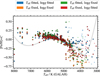 |
Fig. 3 Effects of keeping Teff and log g free parameters or keeping them fixed at the photometric value. Symbols mark the stars belonging to clusters Melotte 25 (circles), Melotte 22 (diamonds), and NGC 2632 (squares). Crosses are measurements for the stars without a trustworthy fit. The solid line is the trend derived in Section 3.4 for the GALAH DR4 iron abundance in dwarfs. |
4.2 Tests
4.2.1 Photometric and spectroscopic Teff and log g
In GALAH DR4, photometric and distance information from Gaia’s 3rd data release (Lindegren et al. 2021; Bailer-Jones et al. 2021) and 2MASS (Skrutskie et al. 2006) are used to estimate Teff and log g, which are then used to better constrain the spectral fit (Buder et al. 2024). For clusters, we are able to get very precise values for Teff and log g (Beeson et al. 2024), which we call photometric temperature and gravity. These are different in DR4 and in this work, because in DR4 all stars in a cluster are treated independently, and here we assume that they must lie on the same isochrone. We test whether the use of precise photometric Teff and log g has any impact on our observed trends. We fitted the spectra with all four combinations, where Teff and log g are either fixed at photometric values or added as completely free parameters. In the latter case, the initial values for the fitting procedure were the photometric values.
In Figure 3 we see that the trends for cool stars follow the same shape as derived from the DR4 data, except in the case where both Teff and log g are free parameters (blue points). The trend plotted in blue sharply diverges from the trends for the other three cases (orange, green, or red points) at Teff = 4500 K. There is also a small difference at around Teff = 6000 K between the fit where log g is fixed and Teff is free (green points in Figure 3) and the other three cases. For stars with Teff > 6000 K, our results are consistent, but do not follow the trend in DR4. In DR4, the trend in this region is constrained mostly by flagged stars, and we only have a small number of observations, so we cannot come to any meaningful conclusions.
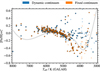 |
Fig. 4 Effect of two different continuum fits on the measured iron abundances. Symbols mark the stars belonging to clusters Melotte 25 (circles), Melotte 22 (diamonds), and NGC 2632 (squares). Crosses are measurements for the stars without a trustworthy fit. The solid line is the trend derived in Section 3.4 for the GALAH DR4 iron abundance in dwarfs. |
4.2.2 Continuum fitting
The GALAH reduction pipeline provides a normalised spectrum, which has been normalised without any prior knowledge of stellar parameters and without the use of a synthetic spectrum. A low order polynomial is fitted to the observed spectrum with several iterations of asymmetric sigma clipping, so the fit represents the upper envelope of the spectrum. Such continuum normalisation is inadequate for abundance analysis, but useful for radial velocity analysis and is used to derive initial stellar parameters with a neural network. With better known stellar parameters and radial velocity, the continuum can be re-fitted later with no loss of information. In the DR4 analysis, the spectra are renormalised at each iteration of the fitting process. This works very well for most stars. However, for cool stars a problem can arise, where there might be no regions in the spectrum where the actual continuum can be sampled (spectra only consist of blended lines). If the continuum levels, temperature, and metallicity are correlated, a wrong combination of these three parameters can produce the best fit and consequently wrong spectroscopic stellar parameters. If the photometric values for Teff can be trusted, and using the literature values for the metallicity of the three well studied clusters, the degeneracy can be broken.
We test whether the iron abundances are different if we dynamically modify the continuum levels (in this case with a polynomial of the 12th order), as in DR4, or if we fit the continuum using photometric Teff, log g, literature metallicity, and DR4 v sin i and vmic. The continuum in the latter case is then kept fixed in the spectral fitting process. In both cases we kept Teff and log g as free parameters. In Figure 4, we see significant differences below Teff < 4500 K. Fixing the continuum produces stronger trends. A dynamic continuum appears to produce trends with a much smaller amplitude than in DR4. This might be a solution to the dip in the trends at around Teff = 3800 K, however, a dynamic continuum also results in the fitted Teff and log g to deviate; significantly from the expected values (see analysis in Section 6 and Figure 13). The degeneracy between Teff, log g and [Fe/H] manifests itself in apparently better [Fe/H] measurements when using a dynamic continuum, but causes issues elsewhere. Hence a dynamic continuum is not a universal solution to any of the problems explored here.
Thresholds for the creation of linelists.
4.2.3 Linelists
The linelist used in GALAH DR4 was adapted from Heiter et al. (2021), which was ultimately produced by VALD (Ryabchikova et al. 2015). In this work we produced our own VALD linelists to have more freedom when experimenting with line depth thresholds as opposed to the curated DR4 linelist with 81 768 entries between 6450 and 6750 Å, which are decreased based on a depth threshold (above 0.001) calculation for each region of the HRD. We produced the linelists by selecting lines based on their depths in spectra of stars with temperatures 3500, 4500, 5500, and 6500 K, vmic = 2 km s−1, and log g = 4.5 and 0.5 (at Teff = 3500 K), log g = 4.5 and 2.5 (at Teff = 4500 K), log g = 4.5 and 4.0 (at Teff = 5500 K), and log g = 4.0 (at Teff = 6500 K). A solar metallicity and composition was used for all linelists. We varied the depth thresholds as given in Table 1 to produce linelists of different sizes. Lines that pass the threshold in at least one of the combinations of above criteria were included in the linelist. Depths of lines were calculated by VALD in spectra produced by the parameters above. The depths are valid for a resolving power of R = 300 000, not for the resolving power of the GALAH spectra. This is not an issue, because we only need to implement some way of thresholding the lines with small depths. The thresholds given in Table 1 are thus arbitrary and were selected so they produce linelists of different sizes. Thresholds in Table 1 show the minimum depth of the line selected from the VALD linelist of a specific temperature. Last column gives the number of lines in the linelist created for the red channel (6450 to 6750 Å).
Many weak lines, individually too weak to pass the threshold for a small linelist, can blend together to produce a significant continuum against which the stronger lines are formed. If this continuum of weak lines is not accounted for in the spectral synthesis, the fit to the observed spectra will be compensated elsewhere, mainly by increasing the metallicity. We expect that by using linelists with insufficient numbers of weak lines, the metallicity and iron abundance will be increased for cool stars. We tested this effect by fitting the spectra using four linelists of different sizes. The results are presented in Figure 5. Limitations of linelists may explain the trends below Teff < 3800 K but not for hotter stars. Above Teff > 5000 K we only see significant deviations when using the smallest (XS) linelist.
A similar issue can arise if linelists are created from lines that only appear in hotter stars. We fitted the spectra using a truncated large linelist (L), produced by omitting lines that would otherwise pass the threshold at 3500 K. We compare iron abundances with the ones obtained with a fit using the full L linelist. Figure 6 shows that the differences appear for stars with Teff < 4500 K. The effect of a truncated linelist is similar to the effect of a small linelist. We chose to use the L linelist instead of the XL linelist to speed up the computations, because L and XL linelist already give very similar results, but L linelist is only half the size of the XL linelist.
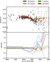 |
Fig. 5 Top: iron abundances computed with linelists of different fidelities. Symbols mark the stars belonging to clusters Melotte 25 (circles), Melotte 22 (diamonds), and NGC 2632 (squares). Crosses are measurements for the stars without a trustworthy fit. The solid line is the trend derived in Section 3.4 for the GALAH DR4 iron abundance in dwarfs. Bottom: difference of iron abundances between the computations using the XL linelist and other three linelists. The solid line shows the median difference in each temperature bin, and the dashed lines show the 16th and 84th percentiles of the differences in each bin. |
4.2.4 Models and spectral fitting codes
SME comes ready with two different stellar atmosphere model grids. MARCS (Gustafsson et al. 2008) is valid for stars with Teff between 3000 and 8000 K, and Atlas/Castelli (Castelli & Kurucz 2003) for Teff between 4000 and 10 000 K. We compared the abundances computed with both grids and found small differences. Iron abundances are lower between 4000 < Teff < 4500 K when calculated using the Atlas/Castelli grid (see Figure 7, top panel).
The trend for iron abundance derived by Korg is remarkably flat. Only below Teff < 3700 K does the iron abundance measured by Korg decrease significantly. The most telling indicator of the difference between the fits produced by SME and Korg are plots of photometric Teff and log g compared to the fitted spectroscopic values as illustrated in Figure 8. Korg’s parameters follow the photometric values much closer and also show no ‘phase shift’ at around Teff = 4500 K. For some stars the spectral fitting did not converge, regardless of the initial conditions. This happens more often with Korg, as one cannot control the boundaries of the fitted parameters in its current implementation. Usually the computed v sin i is much too high. Such stars are marked with crosses in figures discussed in this section, and produce the obvious outliers among the cool stars (e.g. in Figure 8, top panel). Note that we are comparing NLTE abundances derived by SME with LTE abundances derived by Korg. For dwarfs with approximately solar metallicity, the NLTE correction is small, much smaller than the amplitude of the trends that we observe in SME results.
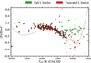 |
Fig. 6 Effects of a truncated linelist on the measured iron abundance. Symbols mark the stars belonging to clusters Melotte 25 (circles), Melotte 22 (diamonds), and NGC 2632 (squares). Crosses are measurements for the stars without a trustworthy fit. The solid line is the trend derived in Section 3.4 for the GALAH DR4 iron abundance in dwarfs. |
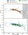 |
Fig. 7 Top: iron abundance obtained with fitting using SME with either MARCS atmospheres or Atlas/Castelli atmospheres. Atlas/-Castelli atmospheres are extrapolated in the grey region. Bottom: comparison of the iron abundance obtained by fitting with SME and with korg. Both use MARCS atmospheres. Symbols mark the stars belonging to clusters Melotte 25 (circles), Melotte 22 (diamonds), and NGC 2632 (squares). Crosses are measurements for the stars without a trustworthy fit. The solid line is the trend derived in Section 3.4 for the GALAH DR4 iron abundance in dwarfs. |
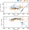 |
Fig. 8 Difference between the spectroscopic and photometric Teff (top) and log g (bottom) for the spectroscopic parameters fitted by SME or Korg. Symbols mark the stars belonging to clusters Melotte 25 (circles), Melotte 22 (diamonds), and NGC 2632 (squares). Crosses are measurements for the stars without a trustworthy fit. |
5 Age verification
5.1 Age determination in the GALAH survey
The analysis of stellar parameters and abundances in GALAH DR4 relies heavily on the photometric information from the Gaia mission. In particular, the log g is estimated from the basic principles, i.e. from the measurements of stellar luminosities (L) (combining Gaia’s photometry and parallaxes), fitted spectroscopic temperatures (Teff), stellar masses (M) and corresponding solar values:
![Mathematical equation: $\[\log~ g=\log~ g_{\odot}+\log \frac{M}{M_{\odot}}+4 ~\log \frac{T_{\mathrm{eff}}}{T_{\mathrm{eff}, \odot}}-\log \frac{L}{L_{\odot}}.\]$](/articles/aa/full_html/2025/11/aa54112-25/aa54112-25-eq5.png) (4)
(4)
Stellar masses are found from the isochrones that best match the observed stellar properties. In DR4 they are interpolated over isochrones with ages between 8 < log(τ/Gyr) < 10.8 in steps of log(Δτ/Gyr) = 0.1, metallicities between −2.75 < [M/H] < 0.75 in steps of 0.25 dex, and then in steps of 0.1 dex to [M/H] = 0.7. Hot stars, evolved white dwarfs and extremely luminous giants are excluded, as they are outside the range of atmospheric models used in spectral fitting. The procedure is performed by the ELLI code (Lin et al. 2018), which also provides stellar ages as a by-product.
For stars in globular clusters, the age has a lower limit of τ > 4.5 Gyr, and for stars in young open clusters, we extend the age range of possible isochrones to log(τ/Gyr) > 6.19; see Buder et al. (2024) for more information.
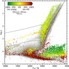 |
Fig. 9 GALAH’s ages of cluster stars compared to isochronal ages. ‘Too young’ means that the GALAH ages are smaller than the isochronal ages, and ‘too old’ means the GALAH ages are larger. Background distribution shows all GALAH DR4 stars. Isochrones for ages 10 Myr, 100 Myr, 1 Gyr, and 10 Gyr and solar metallicity are plotted with solid lines. An isochrone for the age of 10 Gyr and metallicity of [M/H] = −0.5 is plotted with a dashed line. |
5.2 Comparison with isochronal cluster ages
Ages of clusters can be calculated by isochrone fitting, whereby we assume that all stars within a cluster have the same age. So called isochronal ages are much more precise than the age estimates for individual stars as calculated in GALAH DR4. In this work we use isochronal ages of open clusters from Cantat-Gaudin et al. (2020), and Hunt & Reffert (2024) for clusters not in the former catalogue. Ages of globular clusters were taken from Marín-Franch et al. (2009). For young associations and globular clusters we use ages from various literature sources given in Tables A.3 and A.2.
To verify stellar ages, we used all clusters with at least eight stars with a GALAH age. We also excluded ω Cen due to the large age spread of its stellar populations.
We find the GALAH ages are well determined for all stars at the evolutionary stages at and beyond the main sequence turnoff. Among those, the GALAH and literature ages agree best at the turn-off, and in the red clump (Figure 9). On the red giant branch and the asymptotic giant branch, the GALAH ages are typically slightly underestimated (and slightly overestimated on the horizontal branch). On the pre-main sequence there are stars with well estimated ages. However, most stars on the pre-main sequence have ages under- or over-estimated, depending on the position of the pre-main sequence. Stars with correctly estimated ages do not belong to the same clusters, but are rather serendipitous stars that happen to have well matching photometric and spectroscopic parameters, so they get assigned the correct age.
The main lesson learned from the diagrams in Figures 10 and 11 is that seemingly old stars in the GALAH survey are not necessary old. A selection based solely on the age will be polluted by young stars. This might be negligible in practice because there are fewer young than old stars in GALAH DR4, especially among the stars evolved past the main sequence. Although some care is needed when selecting main-sequence stars.
Similarly, by selecting young stars based on the GALAH ages alone, we can miss a large fraction (around a quarter) of the young population. The pollution of such a selection by older stars is mostly negligible in this case.
In addition to systematic errors of ages, we also estimated the statistical uncertainty. To be able to measure the statistical uncertainty without being affected by large systematics, we only used stars within the region marked by the dashed lines in Figure 10. Additionally, we only used clusters that have their mean GALAH age within that region as well. We kept cluster only if at least eight stars remained after the above cuts. We define the one sigma statistical uncertainty as the standard deviation of ages of stars in a cluster divided by the mean GALAH age. We illustrate the results in Figure 12. Globular clusters have typical statistical uncertainties between 10 and 30%. The uncertainty for open clusters varies between 20 and 60% with some outliers among the young clusters. Ignoring the outliers, ages of stars in young clusters have slightly lower uncertainty than in the older clusters. An upper and a lower limit of stellar ages can artificially reduce the measured standard deviations, so the uncertainties in young clusters and in globular clusters might be biased.
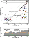 |
Fig. 10 Comparison between GALAH’s ages and isochronal ages. Top: Ages of individual stars in clusters are plotted as small dots (artificially slightly scattered vertically for better perception). The median for each cluster is plotted with a circle of the same colour. Medians marked with a triangle are for clusters with only flagged stars. A one-to-one relation is indicated. A horizontal line separates open clusters from globular clusters. Note a bimodal distribution of GALAH ages for some clusters; one peak is at around 107 yr and another at around 5.0 × 10⁹ yr. Dashed lines mark the region used in the calculation of statistical uncertainties of stellar ages. Bottom: Distribution of stars in log-spaced age bins. Black line shows all stars and the grey area shows unflagged stars. Both distributions are for the whole GALAH DR4 sample. Orange histogram shows the distribution of GALAH ages for cluster members, and the green histogram for individual clusters’ literature ages. A diagram with added cluster names is given in Appendix E. |
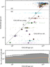 |
Fig. 11 Same as Figure 10, but zoomed into the oldest part of the diagram. The same diagram with added cluster names is given in Appendix E. |
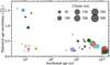 |
Fig. 12 Relative standard deviations of stars in clusters. The colours match those of the clusters in Figures 10 and 11. Symbol size is proportional to the number of GALAH stars in a cluster. Clusters with standard deviation above 1.0 are Gulliver 6, HSC 2907, OCSN 100, OCSN 96, and λ Ori. Large cluster just below 1.0 is Collinder 69. |
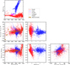 |
Fig. 13 Relationship between photometric Teff and log g, spectroscopic Teff and log g and their respective differences. Red symbols show dwarfs, blue symbols giants, and purple symbols the overlap region. Orange symbols show the averaged values for dwarfs. Only stars with good photometric data are shown. |
6 Verification of Teff and log g
Temperature and surface gravity in GALAH DR4 are computed by spectral fitting using photometric priors. An isochrone that best describes the position of a star on an HR diagram is used to produce a prior for Teff and log g. Because stars are treated independently from each other, a different isochrone might be used to get priors for stars in the same cluster. This could be easily avoided for stars known to be part of a cluster, but most stars in the GALAH survey are not in clusters, so a consistent approach is used where even cluster stars are treated independently.
6.1 Photometric parameters
Here we check how the temperature and surface gravity calculated by isochrone fitting compare to spectroscopic (GALAH DR4) values. To obtain the photometric parameters of stars in clusters, we used literature ages, metallicities, and extinctions to produce2 a Padova isochrone (Bressan et al. 2012; Chen et al. 2014, 2015; Tang et al. 2014; Marigo et al. 2017; Pastorelli et al. 2019) for each cluster. A distance from the isochrone was calculated for each star in a cluster, using Gaia magnitudes. The distance is defined as
![Mathematical equation: $\[d_{\mathrm{CMD}}=\left[\left(M_{G, \mathrm{s}}-M_{G, \mathrm{i}}\right)^2+\left(3\left((B P-R P)_{\mathrm{s}}-(B P-R P)_{\mathrm{i}}\right)\right)^2\right]^{1 / 2},\]$](/articles/aa/full_html/2025/11/aa54112-25/aa54112-25-eq6.png) (5)
(5)
where s indicates the values for a star, and i a value on the isochrone. Absolute magnitudes MG were calculated from Gaia parallaxes. Extinctions of individual stars were not taken into account when calculating distances. Extinction was used to produce the correct isochrone, though. Stars closer to the binary sequence than to the main sequence or pre-main sequence were rejected for having poorly determined photometric parameters. Stars further than 0.5 magnitudes from any part of the isochrone were rejected as outliers. We used the nearest point on the isochrone to determine the photometric parameters for each star.
6.2 Comparison of spectroscopic and photometric parameters
In the comparison described below, we included all clusters that display a well fitted isochrone. The isochrone is defined by the literature values for age, extinction, and metallicity. We further analysed only stars that lie reasonably close to the isochrone (this excludes outliers, blue stragglers, binaries, and stars with peculiar extinction). The results of the comparison are summarised in Figure 13.
A similar pattern is observed for the difference between photometric and spectroscopic parameters vs. temperature as in the trends of abundances of chemical elements. Stars that have photometric temperatures outside the 8000 K > Teff > 3000 K range get squished within these boundaries when a spectroscopic temperature is calculated. This is expected, because, if a star has a temperature in GALAH DR4, it must be within the boundaries of the models used for spectral synthesis. Most of these stars are correctly flagged in DR4. This tension between the photometric and spectroscopic values is illustrated in Figure 14. Vectors point from photometric (Teff, log g) to spectroscopic (Teff, log g), which displays a ‘flow’ in the parameter space. Some coherency in the flow is observed on the RGB and AGB; however, the flow is chaotic on the HB. Correlations are obvious for the dwarfs, as is also evident from Figure 13.
7 Discussion and conclusions
The fourth data release by the GALAH survey marks more than 10 years of operations. DR4 served 1 085 520 spectra of 917 588 stars with parameters that include abundances of up to 32 chemical elements. Although the precision and accuracy of these parameters have improved compared to previous data releases, we observed systematic deviations from expected values. This issue is particularly evident in clusters, which are expected to contain coeval, conatal, and chemically homogeneous populations. Teff and log g are parameters that can be accurately derived from photometric observations of cluster stars with known age, allowing for well-constrained isochrones that the cluster stars should closely follow. Deriving Teff and log g is a complex process that involves finding the isochrone that best describes each star, which defines a photometric prior for Teff and log g. Our initial assumption was that fixing the isochrone for the cluster stars would lead to more consistent measurements of their chemical element abundances. However, this assumption proved to be incorrect because we saw clear systematic abundance trends, which were unrelated to stellar astrophysical processes.
We were unable to identify a single reason for these systematic trends. Our primary focus was on potential issues arising from data processing rather than on possible problems with the understanding and modelling of stellar physics, which will be explored in a future paper. However, we did identify several factors contributing to the systematic errors. Our conclusion that a multitude of factors are responsible for observed systematic errors is in agreement with similar studies in the literature, such as Jofré et al. (2019). The degeneracy between the continuum levels and stellar parameters could be addressed more thoroughly in future analyses, but it remains unclear if this can be resolved at the level of the analysis of the whole survey. More concerning are different results produced by the two spectral fitting codes used in this study, which indicate a significant disagreement between them, even when using the same input parameters.
Consistent measurements of abundances of chemical elements across a wide temperature range are essential for studies where parameters of stars of different temperatures must be compared. Examples are observations of clusters to trace chemical gradients in the Galaxy (Spina et al. 2021) or chemical cartography of the Galaxy (Gaia Collaboration 2023). In such studies, where stars in a large range of distances must be observed, it is inevitable to combine measurements of stars with vastly different temperatures. We showed that abundances, particularly of cool stars, can have systematic errors in the order of 0.5 dex, which is equivalent to the radial metallicity gradient in the Galactic disc over 5 kpc (Spina et al. 2021). It is also essential to be aware of any systematic trends if only a small number of stars are observed in each cluster, as in Zhang et al. (2022), because the systematic trends might not be as easy to derive from sparse observations. As an example of the severity of the problem, we plot a [Fe/H] vs. [Si/Fe] diagram (Figure 15). Si is an element with strong trends (see Figure D.1) and significantly affects the Tinsley-Wallerstein diagram, if we use it as a proxy for α elements abundance.
Machine learning techniques used to derive stellar parameters from spectra (e.g. Ness et al. 2015; Fabbro et al. 2018; Leung & Bovy 2019; Buder et al. 2018) are very sensitive to any systematic errors in the training set. Fixing any non-physical trends, as we show is possible with clusters, could improve the range and reliability of machine learning techniques for parameter derivation. In applications where labels from one dataset are passed and applied to another, such as training a large low-resolution survey on parameters derived in a small overlap with a high-resolution survey (Das et al. 2025; Ambrosch et al. 2023; Nepal et al. 2023), some care for the accuracy and zero-points should be made. Consistency of abundance measurements is also essential for any non-supervised machine learning methods, such as clustering or chemical tagging studies. Chemical tagging in the Galactic disc is challenging, if it is even possible, with the precision of abundances of chemical elements at the level of chemical homogeneity of open clusters (~0.03 dex, Casamiquela et al. 2021; Spina et al. 2022). Hence, consistent measurements with systematic errors corrected at the same level should ideally be used to chemically cluster or tag stars across a large temperature range (Poovelil et al. 2020).
The application of chemical clocks is another example where it is of utmost importance that abundances of chemical elements are measured consistently among stars at different evolutionary stages (Storm & Bergemann 2023; Hayden et al. 2022). Connecting the chemical signatures observed in clusters with the theory of star formation similarly requires observations of a range of stars across the HRD (Kos et al. 2021; Griggio et al. 2022).
In this study, we adopted an empirical approach to address the challenge of achieving consistent measurements of spectroscopic parameters. An open problem remains: how to achieve consistency and precision without empirical ad hoc corrections, but with models and stellar physics (e.g. Spina et al. 2020) used in spectral synthesis codes (Wheeler et al. 2023). This is undoubtedly a complex and extensive problem that will require collaboration and a diverse range of expertise. What is also needed are methods for verifying the codes and models in real data, taken with a variety of instruments in an increasingly larger region of the Universe, in the Galaxy and beyond. We demonstrate that clusters serve as an effective testing ground; in fact, they may be even more powerful than what we have shown here, as the observations of clusters in the GALAH survey were not originally designed for benchmarking purposes.
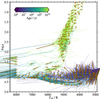 |
Fig. 14 Illustration of the photometric and spectroscopic Teff and log g. Arrows point from the photometric values to the spectroscopic values. Thin lines show the value pairs for each star, and orange arrows for the average flow in that region. Photometric temperatures are sometimes far outside the plotted range, which explains the lines coming from outside of the panel. |
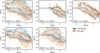 |
Fig. 15 [Fe/H] vs. [Si/Fe] diagrams for stars in different temperature bins. Contours show the density of stars in GALAH DR4 table (blue) and in the detrended table produced in this work (ornage). Stars outside the lowest contour are plotted as points. The grey line shows the general shape of the diagram, so it is easier to compare the positions and shapes of the contours in each panel. Only stars with flag_sp< 4 and with no flags in Iron or Silicon abundances are plotted. |
Data availability
In this work, we produced fitted functions that represent the observed trends in the measurements of abundances of chemical elements in the fourth data release of the GALAH survey. The parameters of the functions are given in Appendix B and are valid for GALAH DR4 only. We also produced a detrended DR4 catalogue of stellar parameters. It is available at the CDS via https://cdsarc.cds.unistra.fr/viz-bin/cat/J/A+A/703/A104 or at https://www.galah-survey.org/dr4/overview/. Table F.1 is also only available in electronic form at the CDS.
Acknowledgements
We acknowledge the traditional owners of the land on which the AAT and ANU stand, the Gamilaraay, the Ngunnawal and the Ngambri peoples. We pay our respects to Elders, past and present, and are proud to continue their tradition of surveying the night sky in the Southern hemisphere. JK, GT and TZ are supported by the Slovenian Research Agency ARIS grants P1-018. TZ acknoledges support of the European Space Agency (Prodex Experiment Arrangement no. 4000142234). GT acknoledges support of the European Space Agency (Prodex Experiment Arrangement no. 4000143450). This work has made use of the VALD database, operated at Uppsala University, the Institute of Astronomy RAS in Moscow, and the University of Vienna.
Appendix A List of clusters
Table A.1 lists open clusters used in this work. Nlit is the number of members in the literature (Cantat-Gaudin et al. (2020) or Hunt & Reffert (2024)), NGALAH is the number of members observed in the GALAH survey. We give the number of all stars, and a number of stars with unflagged spectra in the GALAH survey. Age and extinction (AV) are obtained from Cantat-Gaudin et al. (2020) or Hunt & Reffert (2024) if cluster is not in the former catalogue.
Table A.2 lists globular clusters used in this work. NGALAH is the number of members observed in the GALAH survey. Age and metallicity are literature values.
Table A.3 lists young associations used in this work. Data for Vela OB2 association is taken from Cantat-Gaudin et al. (2019), data for Orion from Kos et al. (2019) and Kos et al. (2021) (with the exception for the age range of Ori OB1cd), and data for Sco-Cen-Crux is taken from Žerjal et al. (2023). If a group or population is made of subgroups with different ages, an age range is given.
Appendix B Trends
Tables B.1 and B.2 provide the knots and coefficients to reproduce the trends derived in Section 3. For elements not included in the tables, there were not enough data to produce meaningful trends. Trends are valid between temperatures given by the first and last knot (in kelvin). Trends are well constrained between 3500 < Teff < 6500 K, and estimated to our best ability outside of these regions. We leave it to the readers discretion to decide in which temperature range they will use our trends. Instructions on how to evaluate the splines given by a list of knots and coefficients are given in the following section.
Open clusters used in this work.
Globular clusters used in this work.
Young associations used in this work.
Knots and coefficients for trends fitted to dwarfs.
Knots and coefficients for trends fitted to giants.
Appendix C Reproducing fitted trends
We represented the trends with cubic splines, as described in Section 3. Tables B.1 and B.2 provide a set of coefficients ci and knots ti for each element. The function describing a trend can be constructed as a sum of weighted base functions:
![Mathematical equation: $\[S(x)=\sum_i c_i B_{i, n}(x),\]$](/articles/aa/full_html/2025/11/aa54112-25/aa54112-25-eq7.png) (C.1)
(C.1)
where base functions Bi,n(x) are defined recursively:
![Mathematical equation: $\[B_{i, 0}(x)= \begin{cases}1, & \text { if } t_i \leq x<t_{i+1}, \\ 0, & \text {otherwise}.\end{cases}\]$](/articles/aa/full_html/2025/11/aa54112-25/aa54112-25-eq8.png) (C.2)
(C.2)
![Mathematical equation: $\[B_{i, k}(x)=\frac{x-t_i}{t_{i+k}-t_i} B_{i, k-1}(x)+\frac{t_{i+k+1}-x}{t_{i+k+1}-t_{i+1}} B_{i+1, k-1}(x),\]$](/articles/aa/full_html/2025/11/aa54112-25/aa54112-25-eq9.png) (C.3)
(C.3)
and k is the order of the spline (k = 3 for a cubic spline in our case).
Below is a Python code to produce trends from a list of coefficients and a list of knots, as given in tables B. 1 and B.2. The code is adapted from https://docs.scipy.org/doc/scipy/reference/generated/scipy.interpolate.BSpline.html. Variable x is a proxy for temperature in Kelvins. Function bspline returns the value for a trend as a function of temperature. t is a list of knots, and c is a list of coefficients.
def B(x, k, i, t):
    if t[i+k] == t[i]:
        c1 = 0.0
    else:
        c1 = (x - t[i])/(t[i+k] - t[i]) * B(x, k-1, i, t)
    if t[i+k+1] == t[i+1]:
        c2 = 0.0
    else:
        c2 = (t[i+k+1] - x)/(t[i+k+1] - t[i+1]) * B(x, k-1, i+1, t)
    return c1 + c2
def bspline(x, t, c):
    k = 3 # spline order (cubic spline)
    n = len(t) - k - 1
    assert (n >= k+1) and (len(c) >= n)
    return sum(c[i] * B(x, k, i, t) for i in range(n))
Appendix D Trends for all elements
Here we plot the trends for all elements. Trends are shown separately for dwarfs and giants (Figures D.1 and D.2, respectively), for unflagged stars only and for all stars together (solid and dashed lines, respectively). Note that the lines showing the trends for flagged and unflagged stars often overlap. Microturbulence and rotational velocity as a function of temperature is also shown in the last two panels.
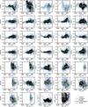 |
Fig. D.1 Trends of abundances of 32 chemical elements in dwarfs. Each panel shows the trends of abundances vs. effective temperature for one element, starting with Fe, and then continuing from small to large atomic numbers. Last couple of panels show the relations between microturbulence velocity (vmic), and rotational velocity (v sin i) vs. effective temperature. Black points represent unflagged stars, grey crosses represent flagged stars. The solid lines are trends fitted on unflagged stars only, and dashed lines are trends fitted to all stars. |
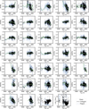 |
Fig. D.2 Trends of abundances of 32 chemical elements in giants. Each panel shows the trends of abundances vs. effective temperature for one element, starting with Fe, and then continuing from small to large atomic numbers. Last couple of panels show the relations between microturbulence velocity (vmic), and rotational velocity (v sin i) vs. effective temperature. Black points represent unflagged stars, grey crosses represent flagged stars. The solid lines are trends fitted on unflagged stars only, and dashed lines are trends fitted to all stars. |
Appendix E Age verification
Figures E.1 and E.2 are the same as Figures 10 and 11, except that they show the names of the clusters as well.
Appendix F Stars and clusters used in tests
To search for the origin of the trends, we re-analysed a small selection of stars while varying parameters and models used in spectral fitting. Because the spectral fitting as done in this work is a slow process, we did not perform it for all clusters. Instead we selected three clusters (Melotte 22, Melotte 25, and NGC 2632) that show all the trends that we would like to explore. Additionally, these three clusters have good quality spectra over a large range of temperatures and complement each other at temperature ranges where one cluster might not have many stars. Stars in these three clusters have well determined age, and have a very similar metallicity.
Because we re-analysed a small subsample of all cluster stars, we took more care about which stars are suitable for the re-analysis. The selection is described in Section 4.1. In this appendix we illustrate the final selection of stars in Melotte 22, Melotte 25, and NGC 2632 (Figures F.1 to F.3) and provide a table of basic parameters and reasons for the rejection of stars (Table F.1).
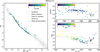 |
Fig. F.1 Stars observed in Melotte 22 and suitable for the analysis of the origin of the trends. Left panel shows the CMD of literature members with stars observed in GALAH marked with coloured symbols. The right two panels show Teff, log g, and iron abundance from the DR4. Additionally, the χ2 of the spectral fitting in DR4 and S/N of the spectra are shown with colours. The isochrone in the left and bottom panels is a Padova isochrones with parameters from Cantat-Gaudin et al. (2020). Stars that might not be reliable for the re-analysis in the search of the origin of the trends are marked with crosses. The reasons why each star was rejected are given Table F.1. |
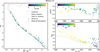 |
Fig. F.2 Same as Figure F.1 but for Melotte 25. |
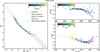 |
Fig. F.3 Same as Figure F.1 but for NGC 2632. |
Example of a list of observed stars in clusters Melotte 22, Melotte 25, and NGC 2632. Last column gives remarks on stars that were observed and analysed in DR4, but rejected for the analysis regarding the origin of the trends. Full table is available online.
References
- Adibekyan, V., Sousa, S. G., Santos, N. C., et al. 2020, A&A, 642, A182 [NASA ADS] [CrossRef] [EDP Sciences] [Google Scholar]
- Amarsi, A. M., & Asplund, M. 2017, MNRAS, 464, 264 [Google Scholar]
- Amarsi, A. M., Asplund, M., Collet, R., & Leenaarts, J. 2016, MNRAS, 455, 3735 [NASA ADS] [CrossRef] [Google Scholar]
- Amarsi, A. M., Lind, K., Osorio, Y., et al. 2020, A&A, 642, A62 [EDP Sciences] [Google Scholar]
- Ambrosch, M., Guiglion, G., Mikolaitis, Š., et al. 2023, A&A, 672, A46 [NASA ADS] [CrossRef] [EDP Sciences] [Google Scholar]
- Asplund, M., Grevesse, N., Sauval, A. J., & Scott, P. 2009, ARA&A, 47, 481 [NASA ADS] [CrossRef] [Google Scholar]
- Asplund, M., Amarsi, A. M., & Grevesse, N. 2021, A&A, 653, A141 [NASA ADS] [CrossRef] [EDP Sciences] [Google Scholar]
- Bailer-Jones, C. A. L., Rybizki, J., Fouesneau, M., Demleitner, M., & Andrae, R. 2021, AJ, 161, 147 [Google Scholar]
- Beeson, K. L., Kos, J., de Grijs, R., et al. 2024, MNRAS, 529, 2483 [NASA ADS] [CrossRef] [Google Scholar]
- Bovy, J. 2016, ApJ, 817, 49 [NASA ADS] [CrossRef] [Google Scholar]
- Bressan, A., Marigo, P., Girardi, L., et al. 2012, MNRAS, 427, 127 [NASA ADS] [CrossRef] [Google Scholar]
- Buder, S., Sharma, S., Kos, J., et al. 2021, MNRAS, 506, 150 [NASA ADS] [CrossRef] [Google Scholar]
- Buder, S., Asplund, M., Duong, L., et al. 2018, MNRAS, 478, 4513 [Google Scholar]
- Buder, S., Kos, J., Wang, E. X., et al. 2024, arXiv e-prints [arXiv:2409.19858] [Google Scholar]
- Cabrera-Ziri, I., & Conroy, C. 2022, MNRAS, 511, 341 [NASA ADS] [CrossRef] [Google Scholar]
- Cantat-Gaudin, T., Mapelli, M., Balaguer-Núñez, L., et al. 2019, A&A, 621, A115 [NASA ADS] [CrossRef] [EDP Sciences] [Google Scholar]
- Cantat-Gaudin, T., Anders, F., Castro-Ginard, A., et al. 2020, A&A, 640, A1 [NASA ADS] [CrossRef] [EDP Sciences] [Google Scholar]
- Casali, G., Magrini, L., Frasca, A., et al. 2020, A&A, 643, A12 [NASA ADS] [CrossRef] [EDP Sciences] [Google Scholar]
- Casamiquela, L., Castro-Ginard, A., Anders, F., & Soubiran, C. 2021, A&A, 654, A151 [NASA ADS] [CrossRef] [EDP Sciences] [Google Scholar]
- Castelli, F., & Kurucz, R. L. 2003, in IAU Symposium, 210, Modelling of Stellar Atmospheres, eds. N. Piskunov, W. W. Weiss, & D. F. Gray, A20 [Google Scholar]
- Chen, Y., Girardi, L., Bressan, A., et al. 2014, MNRAS, 444, 2525 [Google Scholar]
- Chen, Y., Bressan, A., Girardi, L., et al. 2015, MNRAS, 452, 1068 [Google Scholar]
- Chen, B., D’Onghia, E., Alves, J., & Adamo, A. 2020, A&A, 643, A114 [NASA ADS] [CrossRef] [EDP Sciences] [Google Scholar]
- Dal Ponte, M., D’Orazi, V., & Bragaglia, A. 2024, in EAS2024, European Astronomical Society Annual Meeting, 1978 [Google Scholar]
- Das, P. B., Zucker, D. B., De Silva, G. M., et al. 2025, MNRAS, 538, 605 [Google Scholar]
- de Jong, R. S., Agertz, O., Berbel, A. A., et al. 2019, The Messenger, 175, 3 [NASA ADS] [Google Scholar]
- De Silva, G. M., Freeman, K. C., Bland-Hawthorn, J., et al. 2015, MNRAS, 449, 2604 [NASA ADS] [CrossRef] [Google Scholar]
- Dotter, A., Conroy, C., Cargile, P., & Asplund, M. 2017, ApJ, 840, 99 [Google Scholar]
- Dutra-Ferreira, L., Pasquini, L., Smiljanic, R., Porto de Mello, G. F., & Steffen, M. 2016, A&A, 585, A75 [NASA ADS] [CrossRef] [EDP Sciences] [Google Scholar]
- Fabbro, S., Venn, K. A., O’Briain, T., et al. 2018, MNRAS, 475, 2978 [Google Scholar]
- Fu, X., Bragaglia, A., Liu, C., et al. 2022, A&A, 668, A4 [NASA ADS] [CrossRef] [EDP Sciences] [Google Scholar]
- Gaia Collaboration (Recio-Blanco, A., et al.) 2023, A&A, 674, A38 [CrossRef] [EDP Sciences] [Google Scholar]
- Gerber, J. M., Magg, E., Plez, B., et al. 2023, A&A, 669, A43 [NASA ADS] [CrossRef] [EDP Sciences] [Google Scholar]
- Grassitelli, L., Fossati, L., Langer, N., et al. 2015, A&A, 584, L2 [NASA ADS] [CrossRef] [EDP Sciences] [Google Scholar]
- Gratton, R., Bragaglia, A., Carretta, E., et al. 2019, A&A Rev., 27, 8 [NASA ADS] [CrossRef] [Google Scholar]
- Grevesse, N., Asplund, M., & Sauval, A. J. 2007, Space Sci. Rev., 130, 105 [Google Scholar]
- Griggio, M., Salaris, M., Cassisi, S., Pietrinferni, A., & Bedin, L. R. 2022, MNRAS, 516, 3631 [Google Scholar]
- Grilo, V., Souto, D., Cunha, K., et al. 2024, MNRAS, 534, 3005 [Google Scholar]
- Gustafsson, B., Edvardsson, B., Eriksson, K., et al. 2008, A&A, 486, 951 [NASA ADS] [CrossRef] [EDP Sciences] [Google Scholar]
- Hayden, M. R., Sharma, S., Bland-Hawthorn, J., et al. 2022, MNRAS, 517, 5325 [NASA ADS] [CrossRef] [Google Scholar]
- Heiter, U., Jofré, P., Gustafsson, B., et al. 2015, A&A, 582, A49 [NASA ADS] [CrossRef] [EDP Sciences] [Google Scholar]
- Heiter, U., Lind, K., Bergemann, M., et al. 2021, A&A, 645, A106 [EDP Sciences] [Google Scholar]
- Hunt, E. L., & Reffert, S. 2024, A&A, 686, A42 [NASA ADS] [CrossRef] [EDP Sciences] [Google Scholar]
- Jin, S., Trager, S. C., Dalton, G. B., et al. 2024, MNRAS, 530, 2688 [NASA ADS] [CrossRef] [Google Scholar]
- JofrÃl’, P., Heiter, U., Maia, M. T., et al. 2018, RNAAS, 2, 152 [Google Scholar]
- Jofré, P., Heiter, U., & Soubiran, C. 2019, ARA&A, 57, 571 [Google Scholar]
- Kos, J., Lin, J., Zwitter, T., et al. 2017, MNRAS, 464, 1259 [NASA ADS] [CrossRef] [Google Scholar]
- Kos, J., Bland-Hawthorn, J., Asplund, M., et al. 2019, A&A, 631, A166 [NASA ADS] [CrossRef] [EDP Sciences] [Google Scholar]
- Kos, J., Bland-Hawthorn, J., Buder, S., et al. 2021, MNRAS, 506, 4232 [NASA ADS] [CrossRef] [Google Scholar]
- Krumholz, M. R., McKee, C. F., & Bland-Hawthorn, J. 2019, ARA&A, 57, 227 [NASA ADS] [CrossRef] [Google Scholar]
- Larson, R. B. 1981, MNRAS, 194, 809 [Google Scholar]
- Leung, H. W., & Bovy, J. 2019, MNRAS, 483, 3255 [NASA ADS] [Google Scholar]
- Lewis, I. J., Cannon, R. D., Taylor, K., et al. 2002, MNRAS, 333, 279 [NASA ADS] [CrossRef] [Google Scholar]
- Lin, J., Dotter, A., Ting, Y.-S., & Asplund, M. 2018, MNRAS, 477, 2966 [CrossRef] [Google Scholar]
- Lind, K., Asplund, M., & Barklem, P. S. 2009, A&A, 503, 541 [NASA ADS] [CrossRef] [EDP Sciences] [Google Scholar]
- Lind, K., Asplund, M., Barklem, P. S., & Belyaev, A. K. 2011, A&A, 528, A103 [NASA ADS] [CrossRef] [EDP Sciences] [Google Scholar]
- Lindegren, L., Klioner, S. A., Hernández, J., et al. 2021, A&A, 649, A2 [EDP Sciences] [Google Scholar]
- Loaiza-Tacuri, V., Cunha, K., Souto, D., et al. 2023, MNRAS, 526, 2378 [NASA ADS] [CrossRef] [Google Scholar]
- Magic, Z., Collet, R., Asplund, M., et al. 2013, A&A, 557, A26 [NASA ADS] [CrossRef] [EDP Sciences] [Google Scholar]
- Magrini, L., Viscasillas Vázquez, C., Spina, L., et al. 2023, A&A, 669, A119 [NASA ADS] [CrossRef] [EDP Sciences] [Google Scholar]
- Marigo, P., Girardi, L., Bressan, A., et al. 2017, ApJ, 835, 77 [Google Scholar]
- Marín-Franch, A., Aparicio, A., Piotto, G., et al. 2009, ApJ, 694, 1498 [Google Scholar]
- Martell, S. L., Sharma, S., Buder, S., et al. 2017, MNRAS, 465, 3203 [CrossRef] [Google Scholar]
- Mashonkina, L., Gehren, T., & Bikmaev, I. 1999, A&A, 343, 519 [NASA ADS] [Google Scholar]
- Mashonkina, L., Korn, A. J., & Przybilla, N. 2007, A&A, 461, 261 [NASA ADS] [CrossRef] [EDP Sciences] [Google Scholar]
- Massari, D., Mucciarelli, A., Dalessandro, E., et al. 2017, MNRAS, 468, 1249 [Google Scholar]
- Milone, A. P., & Marino, A. F. 2022, Universe, 8, 359 [NASA ADS] [CrossRef] [Google Scholar]
- Moedas, N., Deal, M., Bossini, D., & Campilho, B. 2022, A&A, 666, A43 [NASA ADS] [CrossRef] [EDP Sciences] [Google Scholar]
- Monaco, L., Villanova, S., Carraro, G., Mucciarelli, A., & Moni Bidin, C. 2018, A&A, 616, A181 [NASA ADS] [CrossRef] [EDP Sciences] [Google Scholar]
- Muñoz, C., Geisler, D., Villanova, S., et al. 2021, MNRAS, 506, 4676 [CrossRef] [Google Scholar]
- Mészáros, S., Prieto, C. A., Edvardsson, B., et al. 2012, AJ, 144, 120 [CrossRef] [Google Scholar]
- Nepal, S., Guiglion, G., de Jong, R. S., et al. 2023, A&A, 671, A61 [NASA ADS] [CrossRef] [EDP Sciences] [Google Scholar]
- Ness, M., Hogg, D. W., Rix, H. W., Ho, A. Y. Q., & Zasowski, G. 2015, ApJ, 808, 16 [NASA ADS] [CrossRef] [Google Scholar]
- Osorio, Y., & Barklem, P. S. 2016, A&A, 586, A120 [NASA ADS] [CrossRef] [EDP Sciences] [Google Scholar]
- O’Malley, E. M., & Chaboyer, B. 2018, ApJ, 856, 130 [CrossRef] [Google Scholar]
- Pastorelli, G., Marigo, P., Girardi, L., et al. 2019, MNRAS, 485, 5666 [Google Scholar]
- Piskunov, N., & Valenti, J. A. 2017, A&A, 597, A16 [NASA ADS] [CrossRef] [EDP Sciences] [Google Scholar]
- Piskunov, N. E., Kupka, F., Ryabchikova, T. A., Weiss, W. W., & Jeffery, C. S. 1995, A&AS, 112, 525 [Google Scholar]
- Plez, B. 2012, Turbospectrum: Code for spectral synthesis, Astrophysics Source Code Library [record ascl:1205.004] [Google Scholar]
- Poovelil, V. J., Zasowski, G., Hasselquist, S., et al. 2020, ApJ, 903, 55 [NASA ADS] [CrossRef] [Google Scholar]
- Ratzenböck, S., Großschedl, J. E., Möller, T., et al. 2023, A&A, 677, A59 [NASA ADS] [CrossRef] [EDP Sciences] [Google Scholar]
- Reyes, C., Stello, D., Hon, M., et al. 2024, MNRAS, 532, 2860 [NASA ADS] [CrossRef] [Google Scholar]
- Ryabchikova, T., Piskunov, N., Kurucz, R. L., et al. 2015, Phys. Scr, 90, 054005 [Google Scholar]
- Schiavon, R. P., Phillips, S. G., Myers, N., et al. 2024, MNRAS, 528, 1393 [CrossRef] [Google Scholar]
- Sheinis, A., Anguiano, B., Asplund, M., et al. 2015, J. Astron. Telesc. Instrum. Syst., 1, 035002 [NASA ADS] [CrossRef] [Google Scholar]
- Sinha, A., Zasowski, G., Frinchaboy, P., et al. 2024, ApJ, 975, 89 [Google Scholar]
- Sitnova, T. M., Mashonkina, L. I., & Ryabchikova, T. A. 2016, MNRAS, 461, 1000 [Google Scholar]
- Skrutskie, M. F., Cutri, R. M., Stiening, R., et al. 2006, AJ, 131, 1163 [NASA ADS] [CrossRef] [Google Scholar]
- Smith, V. V., & Lambert, D. L. 1990, ApJS, 72, 387 [NASA ADS] [CrossRef] [Google Scholar]
- Smith, V. V., Bizyaev, D., Cunha, K., et al. 2021, AJ, 161, 254 [NASA ADS] [CrossRef] [Google Scholar]
- Spina, L., Nordlander, T., Casey, A. R., et al. 2020, ApJ, 895, 52 [Google Scholar]
- Spina, L., Ting, Y. S., De Silva, G. M., et al. 2021, MNRAS, 503, 3279 [CrossRef] [Google Scholar]
- Spina, L., Magrini, L., Sacco, G. G., et al. 2022, A&A, 668, A16 [NASA ADS] [CrossRef] [EDP Sciences] [Google Scholar]
- Storm, N., & Bergemann, M. 2023, MNRAS, 525, 3718 [NASA ADS] [CrossRef] [Google Scholar]
- Sun, N.-C., de Grijs, R., Cioni, M.-R. L., et al. 2018, ApJ, 858, 31 [NASA ADS] [CrossRef] [Google Scholar]
- Tang, J., Bressan, A., Rosenfield, P., et al. 2014, MNRAS, 445, 4287 [NASA ADS] [CrossRef] [Google Scholar]
- Ting, Y.-S., Conroy, C., Rix, H.-W., & Cargile, P. 2019, ApJ, 879, 69 [Google Scholar]
- Valenti, J. A., & Piskunov, N. 1996, A&AS, 118, 595 [NASA ADS] [CrossRef] [EDP Sciences] [Google Scholar]
- Vasiliev, E., & Baumgardt, H. 2021, MNRAS, 505, 5978 [NASA ADS] [CrossRef] [Google Scholar]
- Vázquez-Semadeni, E., González-Samaniego, A., & Colín, P. 2017, MNRAS, 467, 1313 [NASA ADS] [Google Scholar]
- Virtanen, P., Gommers, R., Oliphant, T. E., et al. 2020, Nat. Methods, 17, 261 [Google Scholar]
- Wehrhahn, A., Piskunov, N., & Ryabchikova, T. 2023, A&A, 671, A171 [NASA ADS] [CrossRef] [EDP Sciences] [Google Scholar]
- Wheeler, A. J., Abruzzo, M. W., Casey, A. R., & Ness, M. K. 2023, AJ, 165, 68 [NASA ADS] [CrossRef] [Google Scholar]
- Wheeler, A. J., Casey, A. R., & Abruzzo, M. W. 2024, AJ, 167, 83 [Google Scholar]
- Zari, E., Brown, A. G. A., & de Zeeuw, P. T. 2019, A&A, 628, A123 [NASA ADS] [CrossRef] [EDP Sciences] [Google Scholar]
- Zari, E., Hashemi, H., Brown, A. G. A., Jardine, K., & de Zeeuw, P. T. 2018, A&A, 620, A172 [NASA ADS] [CrossRef] [EDP Sciences] [Google Scholar]
- Žerjal, M., Ireland, M. J., Crundall, T. D., Krumholz, M. R., & Rains, A. D. 2023, MNRAS, 519, 3992 [CrossRef] [Google Scholar]
- Zhang, R., Lucatello, S., Bragaglia, A., et al. 2022, A&A, 667, A103 [NASA ADS] [CrossRef] [EDP Sciences] [Google Scholar]
While detrending can improve the accuracy of measurements in an individual star if zero-points are correctly chosen, we study populations of stars in clusters in this work, and the improvement of scatter observed in the GALAH survey as a whole. Hence we choose to use ‘precision’ to describe the scatter of parameters observed in some ensemble of stars. Consequently, the goal of this work is to reduce the scatter, i.e improve the precision.
All Tables
Example of a list of observed stars in clusters Melotte 22, Melotte 25, and NGC 2632. Last column gives remarks on stars that were observed and analysed in DR4, but rejected for the analysis regarding the origin of the trends. Full table is available online.
All Figures
|
Fig. 1 Kiel diagram of the stars used to compute the trends. Unflagged stars are plotted with colours and flagged stars with grey crosses. The grey background distribution shoes all stars in GALAH DR4. Regions delineating dwarfs, giants, and the overlap region are marked in red. The equations of all red lines are specified in Equation (1). |
| In the text | |
|
Fig. 2 Trends for several clusters illustrated for a small selection of elements. Top: Trends for seven open clusters and associations. The last row shows the combined measurements. Bottom: Trends for eight open and globular clusters. Quantities in the first column are shifted by the value of [Fe/H] given under the cluster’s name, so they fit into the same plotting range. The coloured points are unflagged stars; grey crosses are flagged stars. The solid line is a fit for unflagged stars; the dashed line is a fit for all stars. Trends fitted to the complete dataset of clusters are different from those in this illustration and are explained in Section 3.4 and Appendix B. |
| In the text | |
|
Fig. 3 Effects of keeping Teff and log g free parameters or keeping them fixed at the photometric value. Symbols mark the stars belonging to clusters Melotte 25 (circles), Melotte 22 (diamonds), and NGC 2632 (squares). Crosses are measurements for the stars without a trustworthy fit. The solid line is the trend derived in Section 3.4 for the GALAH DR4 iron abundance in dwarfs. |
| In the text | |
|
Fig. 4 Effect of two different continuum fits on the measured iron abundances. Symbols mark the stars belonging to clusters Melotte 25 (circles), Melotte 22 (diamonds), and NGC 2632 (squares). Crosses are measurements for the stars without a trustworthy fit. The solid line is the trend derived in Section 3.4 for the GALAH DR4 iron abundance in dwarfs. |
| In the text | |
|
Fig. 5 Top: iron abundances computed with linelists of different fidelities. Symbols mark the stars belonging to clusters Melotte 25 (circles), Melotte 22 (diamonds), and NGC 2632 (squares). Crosses are measurements for the stars without a trustworthy fit. The solid line is the trend derived in Section 3.4 for the GALAH DR4 iron abundance in dwarfs. Bottom: difference of iron abundances between the computations using the XL linelist and other three linelists. The solid line shows the median difference in each temperature bin, and the dashed lines show the 16th and 84th percentiles of the differences in each bin. |
| In the text | |
|
Fig. 6 Effects of a truncated linelist on the measured iron abundance. Symbols mark the stars belonging to clusters Melotte 25 (circles), Melotte 22 (diamonds), and NGC 2632 (squares). Crosses are measurements for the stars without a trustworthy fit. The solid line is the trend derived in Section 3.4 for the GALAH DR4 iron abundance in dwarfs. |
| In the text | |
|
Fig. 7 Top: iron abundance obtained with fitting using SME with either MARCS atmospheres or Atlas/Castelli atmospheres. Atlas/-Castelli atmospheres are extrapolated in the grey region. Bottom: comparison of the iron abundance obtained by fitting with SME and with korg. Both use MARCS atmospheres. Symbols mark the stars belonging to clusters Melotte 25 (circles), Melotte 22 (diamonds), and NGC 2632 (squares). Crosses are measurements for the stars without a trustworthy fit. The solid line is the trend derived in Section 3.4 for the GALAH DR4 iron abundance in dwarfs. |
| In the text | |
|
Fig. 8 Difference between the spectroscopic and photometric Teff (top) and log g (bottom) for the spectroscopic parameters fitted by SME or Korg. Symbols mark the stars belonging to clusters Melotte 25 (circles), Melotte 22 (diamonds), and NGC 2632 (squares). Crosses are measurements for the stars without a trustworthy fit. |
| In the text | |
|
Fig. 9 GALAH’s ages of cluster stars compared to isochronal ages. ‘Too young’ means that the GALAH ages are smaller than the isochronal ages, and ‘too old’ means the GALAH ages are larger. Background distribution shows all GALAH DR4 stars. Isochrones for ages 10 Myr, 100 Myr, 1 Gyr, and 10 Gyr and solar metallicity are plotted with solid lines. An isochrone for the age of 10 Gyr and metallicity of [M/H] = −0.5 is plotted with a dashed line. |
| In the text | |
|
Fig. 10 Comparison between GALAH’s ages and isochronal ages. Top: Ages of individual stars in clusters are plotted as small dots (artificially slightly scattered vertically for better perception). The median for each cluster is plotted with a circle of the same colour. Medians marked with a triangle are for clusters with only flagged stars. A one-to-one relation is indicated. A horizontal line separates open clusters from globular clusters. Note a bimodal distribution of GALAH ages for some clusters; one peak is at around 107 yr and another at around 5.0 × 10⁹ yr. Dashed lines mark the region used in the calculation of statistical uncertainties of stellar ages. Bottom: Distribution of stars in log-spaced age bins. Black line shows all stars and the grey area shows unflagged stars. Both distributions are for the whole GALAH DR4 sample. Orange histogram shows the distribution of GALAH ages for cluster members, and the green histogram for individual clusters’ literature ages. A diagram with added cluster names is given in Appendix E. |
| In the text | |
|
Fig. 11 Same as Figure 10, but zoomed into the oldest part of the diagram. The same diagram with added cluster names is given in Appendix E. |
| In the text | |
|
Fig. 12 Relative standard deviations of stars in clusters. The colours match those of the clusters in Figures 10 and 11. Symbol size is proportional to the number of GALAH stars in a cluster. Clusters with standard deviation above 1.0 are Gulliver 6, HSC 2907, OCSN 100, OCSN 96, and λ Ori. Large cluster just below 1.0 is Collinder 69. |
| In the text | |
|
Fig. 13 Relationship between photometric Teff and log g, spectroscopic Teff and log g and their respective differences. Red symbols show dwarfs, blue symbols giants, and purple symbols the overlap region. Orange symbols show the averaged values for dwarfs. Only stars with good photometric data are shown. |
| In the text | |
|
Fig. 14 Illustration of the photometric and spectroscopic Teff and log g. Arrows point from the photometric values to the spectroscopic values. Thin lines show the value pairs for each star, and orange arrows for the average flow in that region. Photometric temperatures are sometimes far outside the plotted range, which explains the lines coming from outside of the panel. |
| In the text | |
|
Fig. 15 [Fe/H] vs. [Si/Fe] diagrams for stars in different temperature bins. Contours show the density of stars in GALAH DR4 table (blue) and in the detrended table produced in this work (ornage). Stars outside the lowest contour are plotted as points. The grey line shows the general shape of the diagram, so it is easier to compare the positions and shapes of the contours in each panel. Only stars with flag_sp< 4 and with no flags in Iron or Silicon abundances are plotted. |
| In the text | |
|
Fig. D.1 Trends of abundances of 32 chemical elements in dwarfs. Each panel shows the trends of abundances vs. effective temperature for one element, starting with Fe, and then continuing from small to large atomic numbers. Last couple of panels show the relations between microturbulence velocity (vmic), and rotational velocity (v sin i) vs. effective temperature. Black points represent unflagged stars, grey crosses represent flagged stars. The solid lines are trends fitted on unflagged stars only, and dashed lines are trends fitted to all stars. |
| In the text | |
|
Fig. D.2 Trends of abundances of 32 chemical elements in giants. Each panel shows the trends of abundances vs. effective temperature for one element, starting with Fe, and then continuing from small to large atomic numbers. Last couple of panels show the relations between microturbulence velocity (vmic), and rotational velocity (v sin i) vs. effective temperature. Black points represent unflagged stars, grey crosses represent flagged stars. The solid lines are trends fitted on unflagged stars only, and dashed lines are trends fitted to all stars. |
| In the text | |
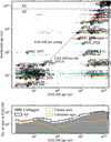 |
Fig. E.1 Same as Figure 10 but with marked names of some prominent clusters. |
| In the text | |
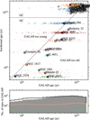 |
Fig. E.2 Same as Figure 11 but with marked names of some prominent clusters. |
| In the text | |
|
Fig. F.1 Stars observed in Melotte 22 and suitable for the analysis of the origin of the trends. Left panel shows the CMD of literature members with stars observed in GALAH marked with coloured symbols. The right two panels show Teff, log g, and iron abundance from the DR4. Additionally, the χ2 of the spectral fitting in DR4 and S/N of the spectra are shown with colours. The isochrone in the left and bottom panels is a Padova isochrones with parameters from Cantat-Gaudin et al. (2020). Stars that might not be reliable for the re-analysis in the search of the origin of the trends are marked with crosses. The reasons why each star was rejected are given Table F.1. |
| In the text | |
|
Fig. F.2 Same as Figure F.1 but for Melotte 25. |
| In the text | |
|
Fig. F.3 Same as Figure F.1 but for NGC 2632. |
| In the text | |
Current usage metrics show cumulative count of Article Views (full-text article views including HTML views, PDF and ePub downloads, according to the available data) and Abstracts Views on Vision4Press platform.
Data correspond to usage on the plateform after 2015. The current usage metrics is available 48-96 hours after online publication and is updated daily on week days.
Initial download of the metrics may take a while.