| Issue |
A&A
Volume 704, December 2025
|
|
|---|---|---|
| Article Number | A88 | |
| Number of page(s) | 16 | |
| Section | Extragalactic astronomy | |
| DOI | https://doi.org/10.1051/0004-6361/202556565 | |
| Published online | 02 December 2025 | |
Shocked, heated, and now resolved: H2 excitation in the low-luminosity AGN at M58 core with JWST
1
INAF – Osservatorio di Astrofisica e Scienza dello Spazio di Bologna, Via Gobetti 93/3, 40129 Bologna, Italy
2
INAF – Osservatorio Astrofisco di Arcetri, largo E. Fermi 5, 50127 Firenze, Italy
3
Instituto de Astrofísica de la Plata (CONICET–UNLP), Paseo del Bosque, 1900 La Plata, Argentina
4
Facultad de Ciencias Astronómicas y Geofísicas, Universidad Nacional de La Plata, Paseo del Bosque, 1900 La Plata, Argentina
5
Space Telescope Science Institute, 3700 San Martin Drive, Baltimore, MD 21218, USA
6
INAF – Istituto di Radioastronomia, Via Gobetti 101, 40129 Bologna, Italy
7
Dipartimento di Fisica e Astronomia “Augusto Righi”, Università di Bologna, via Gobetti 93/2, 40129 Bologna, Italy
8
Observatorio Astronómico Nacional (OAN-IGN)-Observatorio de Madrid, Alfonso XII 3, 28014 Madrid, Spain
9
Centro de Estudios de Física del Cosmos de Aragón (CEFCA), Plaza San Juan 1, 44001 Teruel, Spain
10
Dipartimento di Fisica e Astronomia, Universitá di Firenze, Via G. Sansone 1, 50019 Firenze, Italy
11
Department of Physics and Astronomy, University of California, Los Angeles, CA 90095-1547, USA
12
I. Physikalisches Institut, Universität zu Köln, Zülpicher Straße 77, 50937 Cologne, Germany
⋆ Corresponding author: This email address is being protected from spambots. You need JavaScript enabled to view it.
Received:
23
July
2025
Accepted:
29
September
2025
Abstract
We present JWST NIRSpec and MIRI MRS observations of the central kiloparsec of M58 (NGC 4579), a nearby galaxy hosting a low-luminosity AGN (LLAGN; Lbol ∼ 1042 erg s−1) with a low-power jet. These data provide an unprecedented view of the warm molecular gas phase and reveal clear signatures of feedback. We detect 44 H2 lines, including bright pure rotational lines (S(1)–S(18)) and rovibrational lines up to ν = 2, probing a wide range of excitation conditions. Excitation diagrams show that rotational lines follow a power-law temperature distribution with an exponential cutoff, consistent with heating by low-velocity shocks. H2 rovibrational lines deviate from thermal models primarily because of sub-thermal excitation at low density. Additionally, there may be a 10% contribution powered by AGN X-ray photons in the nucleus. The dust lanes associated with the spiral inflow appear dynamically undisturbed but show signs of shock heating, while the inner ∼200 pc exhibits turbulent kinematics produced by outflowing molecular gas. These results reveal the subtle yet measurable impact of LLAGN feedback on the interstellar medium, demonstrating that even weak, vertically oriented jets and low radiative accretion rates can perturb molecular gas and regulate nuclear reservoirs. This study highlights JWST’s transformative ability to uncover hidden modes of AGN feedback.
Key words: galaxies: ISM / galaxies: jets / galaxies: nuclei
© The Authors 2025
 Open Access article, published by EDP Sciences, under the terms of the Creative Commons Attribution License (https://creativecommons.org/licenses/by/4.0), which permits unrestricted use, distribution, and reproduction in any medium, provided the original work is properly cited.
This article is published in open access under the Subscribe to Open model. This email address is being protected from spambots. You need JavaScript enabled to view it. to support open access publication.
1. Introduction
Molecular hydrogen (H2), the most abundant molecule in the Universe, is paradoxically difficult to observe directly. As a homonuclear diatomic molecule, it lacks a permanent dipole moment, and its quadrupolar rotational and vibrational transitions are intrinsically weak. These lines arise only when the gas is warm (∼200–5000 K) but not yet dissociated. Diagnostic ratios of pure rotational and rovibrational transitions offer sensitive probes of excitation mechanisms, offering insights into the interplay between the interstellar medium (ISM), star formation (SF), and black hole activity (e.g., Mouri 1994; Roussel et al. 2007).
In active galactic nuclei (AGN), black hole accretion drives complex feedback that affects the ISM of the host galaxy (e.g., Harrison & Ramos Almeida 2024). In high-accretion systems, luminous AGN emit intense radiation producing ionization cones and extended outflows (e.g., Cicone et al. 2014; Brusa et al. 2018). Conversely, low-accretion AGN can show collimated jets or slower winds that mechanically interact with the ISM (e.g., Morganti et al. 2005; Heckman & Best 2014). These radiative and kinetic feedback modes are critical components of cosmological simulations, which require AGN feedback to regulate SF and reproduce black hole–galaxy scaling relations (for a review, see Somerville & Davé 2015).
Outflows driven by AGN are observed to be multiphase from ionized to cold molecular components. Yet, whether this feedback quenches or triggers SF remains debated. Some AGN hosts show suppressed SF or gas depletion (e.g., Lammers et al. 2023; Bertola et al. 2024; García-Burillo et al. 2024), while others lie on or above the main sequence (e.g., Mullaney et al. 2012; Jarvis et al. 2020). Further complicating the picture, radiative and mechanical feedback can act simultaneously (e.g., Harrison et al. 2015), and their impact can vary spatially and temporally within the same galaxy (e.g., Bessiere & Ramos Almeida 2022).
When AGN inject mechanical energy into the ISM, they dominate the excitation of molecular gas. H2 lines thereby become the most luminous mid-IR features, as seen in Stephan’s Quintet (Appleton et al. 2006, 2023). In radio-loud AGN, Spitzer revealed a population of molecular hydrogen emission galaxies (MOHEGs), where warm H2 emission is bright, extended, and decoupled from SF (Ogle et al. 2007, 2010). These galaxies show extreme H2 to polycyclic aromatic hydrocarbon (PAH) ratios indicating shock excitation rather than UV heating. The most plausible driver is mechanical heating from jets, possibly aided by cosmic rays, while X-ray dissociation regions (XDRs) fall short of explaining the observed emission (Ogle et al. 2010).
Low-luminosity AGN (LLAGN; LX < 1042 erg s−1), including low-ionization nuclear emission-line regions (LINERs) and weak Seyferts, are typically powered by radiatively inefficient accretion flows (RIAFs), such as advection-dominated accretion flows (ADAFs) or truncated thin disks (for a review, see Yuan & Narayan 2014). These flows emit little UV radiation but can launch powerful megaparsec-scale jets that affect the intergalactic medium, down to low-power radio jets (Pjet ∼ 1042–1044 erg s−1) confined to galactic scales (e.g., Baldi et al. 2018; Mingo et al. 2019; Pierce et al. 2020; Baldi et al. 2021; Webster et al. 2021). These jets interact with the ISM, driving shocks that excite the gas (e.g., Guillard et al. 2012). Low-luminosity AGN with low-power radio jets are valuable laboratories for studying gentle, long-lived feedback (e.g., Sabater et al. 2019; Kharb & Silpa 2023; Ulivi et al. 2024). Though they lack the dramatic outflows of quasars and powerful radio galaxies, LLAGN dominate the local AGN population and account for most of a black hole’s lifetime (Ho 2008; Novak et al. 2011; Burke et al. 2025). Often dismissed as negligible (Shin et al. 2019), growing evidence suggests that they can drive turbulence and inflate radio bubbles, shocking the multiphase gas on kiloparsec scales (e.g., Alatalo et al. 2011; Mezcua & Prieto 2014; Goold et al. 2024).
Messier 58 (NGC 4579) illustrates the impact of low-power jet feedback on a nearby galaxy. Located in the Virgo Cluster at 21 Mpc, it hosts a LINER nucleus (Balmaverde et al. 2016) powered by an ADAF (Nemmen et al. 2014), which launches a radio jet with an estimated kinetic power of ∼2 × 1043 erg s−1, derived from its 1.4 GHz luminosity (νSν = 1.4 × 1039 erg s−1) and the relation by Cavagnolo et al. (2010). Spitzer IRS observations revealed a bright warm H2 disk extending ∼2.6 kpc (Ogle et al. 2024, hereafter O24). CO observations show disrupted molecular gas lanes spiraling inward toward the nucleus (García-Burillo et al. 2009, hereafter GB09), and Gemini near-IR imaging shows that warm H2 emission is bright along these lanes. Central H2 line ratios indicate thermal excitation (Mazzalay et al. 2013). Jet-driven heating is consistent with simulations where a low-power jet perpendicular to the disk inflates a hot bubble into the ISM (Mukherjee et al. 2016, 2018), driving shocks and exciting H2 as it interacts with dust lanes. The resulting cocoon extends over kiloparsec scales and coincides with suppressed SF (O24).
The proximity of M58 makes it a prototypical system for studying LLAGN feedback, particularly in the context of MOHEGs. We were awarded a comprehensive JWST program totaling ∼17 hours with NIRCam, NIRSpec, and MIRI to dissect jet–SM interactions and construct a multiphase view in this galaxy. JWST’s unprecedented spatial and spectral resolution enables detailed probing of the influence of both jet and ADAF. This paper focus on the excitation and dynamics of warm H2 emission, setting the stage for a deeper understanding of LLAGN feedback. Companion papers will address the ionized gas and PAH emission, completing the multiphase picture.
Throughout this work, we adopt a distance of 21 Mpc based on SN 1989M (Ruiz-Lapuente 1996). All maps are shown with north up and east to the left. We use the notation vup–vlow X(Jlow) for H2 lines, where v and J denote the vibrational and rotational quantum numbers and X indicates the branch (S, Q, or O). Pure rotational lines are denoted simply as S(Jlow).
2. Observations and data analysis
M58 was observed with JWST in June 2024 as part of program 3671 (PI: I.E. López), using the full suite of instruments. JWST integral field units (IFU) observations were carried out as 2 × 2 mosaics with NIRSpec and MIRI MRS. Figure 1 shows an overview of the galaxy with the IFU footprints. NIRSpec observations used the G235H F170LP and G395H F290LP grating and filter pairs, covering 1.66–.27 μm, with each mosaic including two sets of four-point medium cycling dithers, totaling 31 minutes of integration per grating. MIRI MRS data observations cover 5–8 μm and used a four-point dither pattern in slow readout mode, with 1.6 hours total integration, including dedicated background frames. Imaging observations with NIRCam and the MIRI Imager used a combination of narrow-, medium-, and broad-band filters (F200W, F212N, F300M, F335M, F770W, F1000W, F1130W, and F1280W) to trace stellar, H2, and dust emission, providing a broader morphological context and supporting astrometric correction of the IFU data.
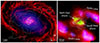 |
Fig. 1. Left: Composite image showing F200W (blue; stellar continuum), continuum-subtracted H2 1– S(1) from F212N (green), and F770W (red; tracing PAH 7.7 μm emission). The LOFAR 144 MHz radio contours are overlaid. The NIRSpec and MIRI Channel 4 fields of view are shown with cyan and yellow dashed lines, respectively. Right: Zoom-in highlighting warm molecular gas traced by H2 S(9) (green), S(1) (red), and CO 2-1 (blue). Overlaid contours are C band from VLA (white) and MERLIN (black). Key regions are labeled, including the northern and southern dust lanes as well as shocked regions to the northeast and southwest. Physical scale bars are shown in both panels. |
Reduction of the datasets followed the JWST Science Calibration Pipeline, with instrument-specific customizations. Full details on data reduction and correction for noise sampling features and fringing are provided in Appendix A. Spectral fitting was performed via multicomponent spaxel modeling, detailed in Appendix B. The velocity center adopted throughout the analysis corresponds to the redshift of the source (vhel = 1518 km s−1).
We used archival MERLIN and VLA C-band (Project ID 20A-272, PI: Ogle) observations to trace the radio structure. The MERLIN map reveals an unresolved 5 GHz core with a flux density of 40±2 mJy beam−1 and a fainter component (2.4 ± 0.5 mJy beam−1). VLA B-configuration imaging shows a jet-like extension on arc second scales, consistent with previous VLA maps (Ho & Ulvestad 2001). Together, the radio data indicate a jet inclined by ∼56° from the plane of the sky. Details of the data reduction are provided in Appendix A. Recent LOFAR 144 MHz observations reveal a large-scale swirling feature, in a counterclockwise direction and opposite to that of the spiral arms, corresponding to the extended jet structure (Edler et al. 2023).
Ultraviolet imaging was obtained with HST, using the ACS/HRC F250W filter (Program ID 9454; PI: Maoz). We combined two exposures and applied an astrometric correction of 0 2 to align the UV core with the MERLIN radio continuum, as the astrometry was limited primarily by guide star uncertainties. The UV morphology reveals a ring-shaped structure interpreted as an ultracompact nuclear ring of young stars with a radius of ∼150 pc (Comerón et al. 2008). We also used Spitzer IRS maps of the H2 S(3) line from O24 and CO(2–1) observations from the Plateau de Bure Interferometer (PdBI) presented by GB09.
3. Results
JWST probes the inner kiloparsecs of M58 with unprecedented detail (Fig. 1). The PAH 7.7 μm emission traces the dusty spiral arms and the inner dust disk. NIRCam F200W imaging maps the old stellar population as a smooth continuum aligned with a ∼ 8 kpc bar and decoupled from the inner dust disk. The F212N narrowband show the H2 1–0 S(1) rovibrational emission confined to the inner 2.6 kpc and consistent with O24. The IFU data cover the central 0.7–1.2 kpc and trace the molecular phase of the ISM around the AGN. Two main dust lanes to the north and south dominate the H2 emission, converging toward the nucleus, in agreement with absorption seen in HST optical images and CO morphology (O24). Closer to the AGN, two regions show enhanced H2 emission: one in the northeast (NE) at ∼100 pc and another in the southwest (SW), partially overlapping the nucleus.
The nuclear spectrum (Fig. 2), extracted within a 1″ aperture (≈100 pc), is dominated by a strong mid-IR continuum and exhibits two prominent silicate emission features (9–13 μm and 15–19 μm). Although the bright continuum partially masks the PAH bands, the 11.3 μm feature is clearly detected. Strong lines from ionized species ([Ne V], [Ar II], [Fe II]) and numerous H2 transitions (pure rotational and high-ν rovibrational lines) indicate a mix of photoionization and mechanical heating. Circumnuclear spectra, extracted from a ring between 1″ and 3″, show that both H2 rotational lines and low-ionization lines ([Ar II], [Fe II], [Ne II], and [S III]) are strong. The CO absorption bands are also detected across the field. A list of all detected H2 lines for the different regions is given in Table C.1.
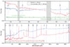 |
Fig. 2. JWST spectra for the nucleus (blue) and for a circumnuclear region (red). Ionic emission lines are indicated by vertical blue lines. The PAH features and H2 lines are marked along the bottom of each panel. The circumnuclear region exhibits strong PAH emission, pure rotational H2, and low-excitation ionized lines. In contrast, the nuclear spectrum shows prominent high-ionization lines, relatively stronger H2 rovibrational lines, and two silicate features at 10 μm and 17 μm. Shaded-gray regions indicate gaps in the NIRSpec instrument. |
Moment maps (Fig. 3) show that H2 emission follows the dust lanes, except for very high-excitation transitions (e.g., ν = 2). The low-ionization line [Ar II] extends within the inner 200 pc and peaks at the AGN. The high-ionization line [Ne V] is confined to ∼100 pc and displays distinct kinematics. The enhanced mid-J H2 emission (e.g., S(5)) relative to lower-J lines (e.g., S(1)) is consistent with O24. However, the presence of higher vibrational levels within ≲100 pc of the AGN suggests that additional excitation sources may contribute (see Section 4). The velocity fields of low-ionization lines and H2 appear broadly consistent, with a ±200 km s−1 difference between the northern and southern lanes. While this may suggest rotation, caution is advised due to noncircular motions driven by the stellar bar (GB09). Nevertheless, the lanes show low velocity dispersion as expected for rotation, whereas the nucleus reaches several hundred km s−1. Ionized and high-excitation H2 lines show elevated dispersions in the nucleus and NE.
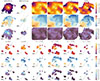 |
Fig. 3. Moment maps showing H2, low-ionization [Ar II], and high-ionization lines [Ne V]. Only pixels with detections above 5σ are shown. The dashed and dotted gray lines indicate the jet axis and the galaxy’s major axis, respectively. A black x marker indicates the AGN radio core. |
The NIRSpec channel maps of the H2 1–0 S(1) and H2 S(9) transitions (Fig. 4) show that the two main dust lanes (north and south) appear in a limited number of bins, with reduced velocity dispersion, consistent with a rotating disk. The northern lane spans –300 to –100 km s−1, while a southern bridge connecting the nucleus to the southern lane appears between –200 and –100 km s−1. The main southern lane itself spans from –100 to +200 km s−1. The NE feature is strongest at –500 km s−1 and persists up to +200 km s−1. The AGN nucleus emits across nearly all bins, showing high velocity dispersion and indicating broad, turbulent motions. The emission shows a complex morphology: it starts as a vertical column between –500 and –300 km s−1, takes on a curved arc shape across most bins, and eventually splits into two lobes at its outer edges above +200 km s−1.
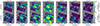 |
Fig. 4. NIRSpec channel maps, illustrating both rotational and rovibrational kinematics. Top row: H2 1–0 S(1); Bottom row: H2 S(9). Each column corresponds to a velocity bin (from –500 to +500 km s−1). A dashed white line represents the jet axis. Both transitions trace the dust lanes between –300 to +200 km s−1, compatible with rotation. The NE feature, strongest at –500 km s−1 and persisting to +200 km s−1, is identified as the forward shock front. The overall lack of alignment with the jet axis suggests the jet passes outside the disk plane. |
We do not find any strong alignment of velocity features with the jet axis, implying that the jet propagates largely out of the disk plane and has limited direct impact on the molecular disk. However, the systematic detection of NE and SW emission across many velocity channels, and across all H2 transitions from low to high excitation, points to the presence of an ongoing shock front roughly perpendicular to the jet axis, likely driven by a bubble inflated by the radio jet. Finally, while outflows are proposed in GB09 and O24, we detect no high-velocity flows (v > 600 km s−1) in either the molecular or ionized gas. Nonetheless, modest outflow velocities are examined in Section 5.
4. H2 excitation
Warm H2 in galaxy centers can arise from a variety of excitation mechanisms. In this section, we use spatially resolved diagnostics, excitation modeling, and multiwavelength context to constrain the dominant heating mechanisms and its origin.
4.1. Pure rotational H2 lines
Previous work by O24 showed that the ionized gas in M58’s nucleus is shock-excited, with shock velocities of 170–440 km s−1. Warm molecular gas was inferred to be similarly heated based on an elevated H2/PAH ratio. While such a ratio is useful in integrated analyses, H2 and PAHs often arise from distinct regions. However, spatial variations in the ratio can still reveal where one emission dominates (e.g., García-Bernete et al. 2024). With JWST’s improved spatial and spectral resolution, we use more physically motivated diagnostics.
We adopted the S(3)/S(1) ratio as our primary tracer of excitation (Fig. 5), due to its sensitivity to temperature and weak dependence on extinction (Lambrides et al. 2019). Since S(3) arises from a higher energy level than S(1), the ratio steeply increases with temperature. In typical SF regions as M58’s spiral arms, S(3)/S(1) is approximately 0.6 (O24), while in the photodissociation regions (PDRs) of the Orion molecular cloud (OMC), it averages 1.36 (Van De Putte et al. 2024). We find S(3)/S(1) > 1.5 along the dust lanes and up to ∼5 near the AGN, forming NE–SW lobes roughly perpendicular to the jet. To probe hotter gas, we used S(9)/S(5) and S(13)/S(7). These ratios range from 0.1–0.3 in the dust lanes and increase to 0.3–0.5 in the lobes. The nucleus indicates that S(13)/S(7) is approximately 0.25–0.30, spatially confined within ∼20 pc of the AGN, and the NE lobe has lower values. In S(9)/S(5), the NE lobe traces a clear arc of enhanced excitation, marginally seen in S(13)/S(7).
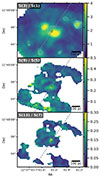 |
Fig. 5. Maps of pure H2 rotational line ratios. Top: S(3)/S(1) show elevated values in the dust lanes and in two-lobed structures near the AGN. White contours represent the OPR; the outermost contour corresponds to 3 (expected in LTE at T ≳ 200 K), with inner contours decreasing in steps of 0.25 down to 1.5. Middle: S(9)/S(5). Bottom: S(13)/S(7). These ratios reveal that the higher-J lines trace arc-like structures in both lobes. The dashed gray line indicates the jet axis. |
We compare these results to C-and J-type shock models from Kristensen et al. (2023), adopting pre-shock densities of nH = 102–103 cm−3 and a magnetic field strength of B = 30 μG, consistent with O24. The external UV radiation field G0 spans a wide range of conditions (1-100), from diffuse clouds to shocked extragalactic environments (Wakelam et al. 2017). Only C-type shocks are able to reproduce the observed H2 line ratios, that primarily depend on shock velocity and density, with only minor sensitivity to external parameters such as G0 or cosmic-ray ionization rates (Fig. 6). The S(3)/S(1) ratio increases steeply with shock velocity across the entire range of parameters. The S(9)/S(5) and S(13)/S(7) ratios match the observed values at low velocities (≲10–30 km s−1) in all regions and at higher velocities (≳50 km s−1) only in the dust lanes. Taken together, these trends consistently point to low-velocity C-type shocks in relatively low-density gas as the dominant H2 excitation mechanism. Alternative mechanisms such as UV pumping preferentially enhance vibrational lines and have minimal impact on low-level ν = 0 lines such as S(3). Likewise, variations in the H2 cosmic-ray ionization rate have negligible effect. We further discuss these alternatives for rovibrational excitation in Section 4.4.
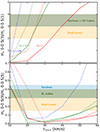 |
Fig. 6. Predicted pure H2 rotational line ratios as a function of shock velocity, based on the C-type shock models of Kristensen et al. (2023). Two model sets are shown with a magnetic field strength of B = 30 μG and pre-shock densities of nH = 100 cm−3 (solid lines) and nH = 1000 cm−3 (dashed lines). Colored curves indicate different strengths of the external UV radiation field G0. Shaded regions mark the range of observed ratios. Constraints on S(13)/S(7) are similar to those for S(9)/S(5). |
4.2. Ortho-to-para ratio
Figure 5 also overlays contours of the H2 ortho-to-para ratio (OPR), defined as the ratio of ortho-H2 (odd rotational levels, J = 1, 3, 5, …) to para-H2 (even levels, J = 0, 2, 4, …). We derive the OPR directly from the measured column densities of the ortho transitions (S(1)–S(7)) and the para transitions (S(2)–S(8)) and report it for regions where all eight rotational lines are detected, ensuring a good sampling across a wide temperature range. However, the absence of S(0) in the JWST coverage reduces our sensitivity to any very cold, para-rich reservoir.
In local thermodynamic equilibrium (LTE) at T ≳ 200 K, proton-exchange reactions drive the OPR toward 3 (Reeves & Harteck 1979). Across most of the inner kiloparsec, we measure OPR values consistent with this equilibrium, indicating that the H2 has either formed under or relaxed into LTE conditions. However, several compact regions show significantly lower values (OPR ∼ 1.5–2). These include the vicinity of the AGN, encircling the SW lobe and the NE lobe. These regions also exhibit disturbed kinematics (Fig. 4) and likely trace the aftermath of shock fronts. Additional low-OPR regions are found along the dust lanes. Departures from the equilibrium value can naturally arise when H2 has been dissociated and subsequently reformed on dust grains, yielding a sub-equilibrium OPR. The ratio then evolves gradually toward 3 via proton-exchange reactions, with characteristic timescales of ∼105–107 yr depending on the gas ionization fraction and density (Wilgenbus et al. 2000; Flower et al. 2006). The observed sub-equilibrium OPR values therefore likely mark sites of recent H2 reformation or ongoing thermal relaxation following shock passage, consistent also with model predictions from Kristensen et al. (2023).
4.3. Modeling excitation diagrams
To better characterize the warm H2 excitation, we constructed excitation diagrams in each spaxel of the field of view. Plotting the column density per statistical weight, (Nu/gu), against upper-level energy Eu, and assuming optically thin emission and LTE, allowed us to infer the temperature distribution and total column density of the warm H2. While several regions show OPR values below the LTE value, Ogle et al. (2010) showed these deviations have minimal impact on temperatures and masses derived from such diagrams. We used a continuous power-law temperature distribution model introduced by Togi & Smith (2016), which assumes dN/dT ∝ T−n with T ≥ Tl, where n is the power-law index and Tl is the lower cutoff temperature. Low Tl values (e.g., 50–100 K) are indicative of heating typical of PDRs, while higher values (≳200 K) suggest shock or turbulence-driven heating. For comparison, measurements of M58’s spiral arms from O24 yield Tl ∼ 50 K, consistent with PDRs.
We find that the original implementation from Togi & Smith (2016) underpredicts the fluxes of high-excitation lines starting at S(11), as it truncates the temperature distribution at T = 2000 K. High-J lines are sensitive to hotter gas (T > 3000 K), which the model excludes. Although two-temperature models can capture this component, they impose an arbitrary separation. To maintain a continuous and physically consistent description, we extended the integration up to the H2 dissociation limit (T = 5000 K). Because H2 begins to thermally dissociate between ∼4000–5000 K (Hollenbach & Tielens 1999), we introduced an exponential cutoff to suppress unphysical contributions at extreme temperatures. The modified distribution becomes
 (1)
(1)
with Tcut = 3500 K as a soft cutoff and Tmax = 5000 K as the upper limit, retaining the flexibility while enforcing a physically motivated suppression near the dissociation threshold.
Figure 7 shows the fitted parameters across the field, and example excitation diagrams for selected regions appear in Fig. 8. The power-law index n indicates the steepness of the temperature distribution: high n implies that cooler gas dominates; low n implies that hot gas dominates. Along the dust lanes, we find high n values (up to ∼6.5), steep temperature distributions, and Tl ∼ 300–350 K. In contrast, regions between the nucleus and lanes show flatter distributions (n ∼ 4–5) and lower Tl ∼ 200 K, with the nucleus having the flattest slope (n ≈ 3.9) and highest cutoff temperature, signaling a dominant hot component likely heated by AGN-driven processes. The NE–SW lobes also reach T ∼ 500 K, indicating a large warm gas contribution. Note that the Tl parameter in the model from Fig. 8 represents a lower bound on the gas temperature.
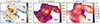 |
Fig. 7. Maps from the modified power-law temperature distribution model from Togi & Smith (2016). Left: Power-law index n, with lower values indicating a stronger contribution from hotter gas. Center: Lower temperature Tl, contributing to H2 emission. Right: Warm H2 mass per pixel, with each pixel area being ≈161 pc2. White contours trace CO(2–1) emission from cooler molecular gas. The dashed gray line marks the jet axis. |
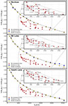 |
Fig. 8. H2 excitation ladders for selected regions. Top: Nucleus. Middle: Northeast shock. Bottom: South lane. Pure rotational H2 lines are shown in blue, with best-fit models in yellow triangles. Observed rovibrational lines are plotted in red, with zoomed-in insets displayed in the top corners of each panel. The solid line connects the 1–0 S(1–7) rovibrational ladder, while the dashed line connects the 1–0 O(2–9) ladder. |
We converted the fitted temperature distributions into warm H2 masses (T > 200 K), following Togi & Smith (2016), using the spaxel area of MRS CH1 (0.0168 arcsec2 or ∼161 pc2). Most warm gas lies in the dust lanes, and a clear disruption in the southern lane is traced by H2, as also seen in CO (GB09) and reflected in kinematics (Fig. 3). Despite their compact size (each lobe spanning roughly 100 pc × 50pc), the two molecular lobes contain a substantial amount of warm H2, each one with approximately 5 × 10⁴ M⊙ of warm H2.
4.4. Rovibrational H2 lines
The excitation diagrams in Figure 8 show clear decoupling between the pure rotational and rovibrational H2 ladders across regions. Were the gas in LTE fit by a single temperature, both sets of transitions would fall along the same curve in a Boltzmann plot. Instead, the ν = 1–0 lines (both S- and O-branches) lie systematically below the rotational trend. High-energy rovibrational lines (e.g., 1–0 S(7), Eu/k ≳ 104 K) align more closely with the rotational ladder, whereas low-energy lines (e.g., 1–0 S(1)) are offset by up to two dex. This curvature, in which the excitation temperature increases with Eu, is characteristic of shock-dominated environments where higher-J and rovibrational transitions preferentially trace hotter gas (Kristensen et al. 2023).
This misalignment has been observed in a variety of galaxies: for instance, NGC 1266 requires mixed PDR and AGN contributions to reproduce its H2 ladder (Otter et al. 2024), and NGC 3256 combines slow shocks and X-ray heating to reach rovibrational temperatures near 2000 K (Emonts et al. 2014). Similarly, protostellar outflows show LTE-like pure rotational lines alongside sub-thermal rovibrational levels in nonequilibrium OPR regions (Vleugels et al. 2025). In M58, the divergence between S and O branches persists even where OPR ≈ 3, confirming that a simple OPR effect cannot account for the offset.
The systematic underpopulation of the ν ≥ 1 transitions relative to the pure rotational ladder demonstrates that a single-temperature model cannot account for both rotational and vibrational lines. Although a temperature distribution of Tu = 150–500 K reproduces the pure rotational data, it overestimates the ν = 1–0 rovibrational line intensities. This discrepancy arises because rovibrational levels have critical densities on the order of ∼106 cm−3 (e.g., v = 1, J = 3 at T ≳ 2000 K), whereas low-J rotational lines require densities of only ≲103 cm−3 (e.g., S(1)). In regions where nH < ncrit, collisions cannot sustain thermal level populations, leading to sub-thermal excitation and correspondingly weaker rovibrational emission. This sub-thermal excitation naturally produces the flattening of the 1–0 S(1-7) ladder, reflecting variations in gas density and excitation depth across the field. However, additional excitation mechanisms may also contribute. The rovibrational lines may arise from gas subject to different shock velocities or irradiated by energetic photons. In particular, photon-driven processes such as UV or X-ray pumping can preferentially populate high vibrational states, modifying the ladder independently of the thermal background.
Another useful diagnostic compares pure rotational with rovibrational lines, such as S(9)/1–0 S(5) and S(13)/1–0 O(7), which can be readily derived from the fluxes listed in Table C.1. These ratios probe different excitation regimes, revealing variations in shock strength and post-shock cooling. The two lanes and the NE region exhibit S(9) dominance (∼1.2). Only the nucleus exhibits an S(9)/1–0 S(5) of ∼0.85, implying hotter conditions with more efficient rovibrational excitation. The S(13)/1–0 O(7) lines are at similar wavelengths, minimizing extinction effects, and trace density in partially thermalized gas. The critical density of S(13) (ncrit ∼ 106 cm−3) is much higher than 1–0 O(7). In the OMC, the ratio is uniformly ∼1.05, indicating full thermalization at ncrit, while in extreme shocked regions it can rise to ∼2.3 due to overpopulated high-J levels under sub-thermal conditions (Brand et al. 1989). In M58, the nucleus reaches peak values of ∼1.95, consistent with high temperatures and sub-thermal excitation, while values ≲1.3 in the dust lanes indicate denser, near-LTE conditions. Together, these trends support a picture of cooler dust lanes and hotter, less dense lobes, with local density variations consistent with turbulent post-shock structures.
Figure 9 presents the 2–1 S(1)/1–0 S(1) versus 1–0 S(2)/1–0 S(0) diagram (e.g., Mouri 1994; Rodríguez-Ardila et al. 2004; Mazzalay et al. 2013), which jointly constrains the vibrational (Tvib) and rotational (Trot) excitation temperatures of the gas1. In LTE and under purely thermal excitation, the line ratios fall along a curve where Tvib ≈ Trot. Deviations can be explained by model predictions for UV and/or X-ray heating, shocks, and when Tvib > Trot, indicating the presence of nonthermal excitation. Although the 2–1 S(1)/1–0 S(1) ratio is often used to identify UV pumped gas, it is sensitive to Tvib and may reflect vibrational thermalization under shock conditions. High Tvib values have been observed in dense shocked clouds such as the OMC (Habart et al. 2005), but in M58 the conditions appear more consistent with a lower-density regime, where collisions are less effective at thermalizing vibrational levels. Under these circumstances, the 2–1/1–0 ratio remains a valid diagnostic of the relative contribution of the thermal versus nonthermal contribution. With all regions showing values below 0.5, we can confidently rule out pure nonthermal fluorescence in M58. Instead, all regions are broadly consistent with collisional excitation driven by shocks. The nucleus and north lane lie closest to the pure thermal curve, consistent with ∼90% thermal and ∼10% nonthermal excitation. The NE and SW lobes shift toward larger nonthermal fractions (∼20–30%). The south lane has weak 2–1 S(1) emission and cannot be fully constrained. These mixed-excitation fractions align with surrounding physical conditions: shocks dominate in the central regions and along the north lane, while the lobes, located between the AGN and the UV ring, experience enhanced radiative excitation. This behavior echoes findings in other LINER and Seyfert 2 galaxies, which typically cluster near the thermal curve with modest nonthermal offsets. This is in contrast to Seyfert 1 and starburst systems, which show stronger fluorescent signatures (Riffel et al. 2013; Otter et al. 2024).
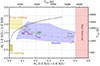 |
Fig. 9. H2 2–1 S(1)/1–0 S(1) vs. 1–0 S(2)/1–0 S(0) emission-line ratios for selected regions of M58. Colored markers indicate the nucleus (Nuc), north and south lane (NL-SL), and the northeast and southwest H2 lobes (NE-SW). The solid black curve marks the predicted trend for pure thermal excitation. Shaded regions represent the domains of alternative excitation mechanisms: UV thermal excitation (Sternberg 1989), X-ray heating (Draine & Woods 1990), shocks (Kristensen et al. 2023), and nonthermal UV fluorescence (Black & van Dishoeck 1987). The gray curve shows mixed thermal and fluorescent excitation models, decreasing from 90% thermal (left) in 10% steps. The top and right axes indicate the vibrational and rotational temperatures (Tvib, Trot) respectively. |
4.5. Origin of H2 excitation
We have shown that the pure rotational lines are nearly fully thermal, while the rovibrational lines contain only a 10–30% nonthermal component. We now assess the physical drivers responsible for these excitation processes.
4.5.1. Thermal dominance
Since low-lying pure-rotational lines dominate thermal H2 cooling, Fig. 10 compares the radial profile of the rotational luminosity, scaled from S(3) to the total S(1)–S(5) emission2 to the energy available from three candidate mechanisms, each assuming a conservative 5% coupling efficiency. We estimated the radio jet’s mechanical power, using VLA 5 GHz and LOFAR 144 MHz maps and the scaling relations of Cavagnolo et al. (2010)3. X-ray heating of the AGN was evaluated using the observed luminosity accounting for r−2 geometric dilution. The cloud–cloud collision power was calculated via  , where Ṁ represents the inflow and outflow rates from GB09, assuming v = 150 km s−1 for cloud encounters.
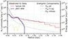 |
Fig. 10. Radial profile of H2 luminosity surface density compared to various energy input mechanisms. Spitzer IRS and JWST MIRI H2 S(3) measurements are scaled to match the total S(1)–S(5) luminosity. The JWST-derived surface density drops beyond 0.5 kpc due to the limited field of view. Energy surface densities, assuming an overall coupling efficiency of η = 5%, are shown for X-ray radiation pressure and kinetic power from cloud–cloud collisions and from the radio jet. |
Even at 5% efficiency, the jet’s kinetic power exceeds the H2 surface brightness across the full 2 kpc. By contrast, X-ray heating is limited to the inner ∼100 pc and cloud–cloud collisions can sustain the emission only beyond ∼1.5 kpc. Even combined, these two processes cannot account for the prominent H2 bump at 0.3–0.4 kpc, coincident with the onset of the dust lanes. Despite the simplified assumption, the radio jet alone provides sufficient energy to power the thermal H2 emission at all scales. Other processes, even if locally relevant, would require implausibly high coupling efficiencies: XDR heating typically operates at ≲1% (Ogle et al. 2010), and while cloud–cloud collisions can be efficient in extreme interacting systems (e.g., Stephan’s Quintet; Guillard et al. 2009), there is no evidence for recent mergers or interactions in M58. We did not explore other origins of the shocks, such as supernova-driven shocks, given the lack of evidence for a past intense starburst. Likewise, the morphology of the shocked region does not support external drivers such as cluster ram pressure (e.g., NGC 4569; Boselli et al. 2016).
4.5.2. Nonthermal contribution
In the nucleus, evidence suggests a nonthermal excitation of ∼10%. Although our excitation grids model nonthermal excitation solely via UV fluorescence, other processes (e.g., cosmic rays and XDRs) could similarly populate the v = 2 level.
The observed nuclear 2–1 S(1) luminosity is L2 − 1S(1) ≈ 3.25 × 1037 erg s−1. This line arises from the level (v = 2, J = 3), typically populated via radiative cascades following UV pumping through electronic transitions (e.g., B1Σu+ → X1Σg+). The probability that an absorbed UV photon ultimately leads to population in v = 2 is set by the Franck–Condon factors, which for v = 2 are ∼0.15 (Spindler 1969). Adopting a conservative 10% cascade efficiency (Sternberg et al. 2014) obtain an overall UV-to-2–1 S(1) conversion efficiency of η ≈ 0.015. From LLAGN models, the intrinsic far-UV luminosity of the AGN is L110nm ≈ 6.68 × 1033 erg s−1 nm−1 (López et al. 2024), corresponding to a photon rate of  ∼ 1.38 × 1042 s−1. Thus, the predicted 2-1 S(1) luminosity is Lpred =
  ≈ 1.83 × 1028 erg s−1, nine orders of magnitude below the observed value. Using HST fluxes that include UV emission from young stars yields similarly low results: extrapolating from 250 nm (Maoz et al. 2005), we estimate L110nm ∼ 1.7 × 1039 erg s−1 nm−1, implying
  ∼ 3.5 × 1047 s−1 and Lpred ∼ 4.7 × 1033 erg s−1. Even assuming perfect trapping, UV fluorescence falls orders of magnitude short. We therefore conclude that UV pumping is negligible for the observed high-v H2 emission in the nucleus.
X-rays penetrate deeper into molecular clouds than UV photons, generating fast photoelectrons that collisionally excite H2 to high vibrational levels. Given the intrinsic AGN X-ray luminosity of LX ∼ 1.6 × 1041 erg s−1 and a clumpy medium with n ∼ 103 cm−3, soft X-rays can be absorbed within a few parsecs, and XDR models predict T ∼ 103 K gas and efficient v = 2 excitation (Draine & Bertoldi 1996). Accounting for the approximately 10% nonthermal 2–1 S(1) emission requires ∼760 M⊙ of warm H2, only approximately 3% of the total T > 200 K gas we infer in the nucleus. Similar warm gas fractions and X-ray-driven H2 rovibrational excitation have been observed in other AGN (e.g., Riffel et al. 2013; Storchi-Bergmann et al. 2009), making X-ray pumping a viable explanation for the nuclear nonthermal component.
Cosmic rays can excite the H2, primarily populating the v = 1 vibrational level (Padovani et al. 2022); however, producing the observed emission would require extremely high ionization rates. Adopting a nonthermal 1–0 S(1) luminosity of 2.41 × 1037 erg s−1 (10% of the total) and a warm H2 reservoir of ∼2.5 × 10⁴ M⊙ at T > 200 K, the required ionization rate is ∼10−10–10−9 s−1, depending on the assumed photon yield per ionization (10−3–10−2). These values are orders of magnitude higher than typical Galactic molecular cloud rates (10−16–10−15 s−1 Indriolo & McCall 2012; Neufeld & Wolfire 2017) and even exceed the highest rates seen in the Galactic Center or strong shocks (∼10−14–10−13 s−1; Padovani et al. 2018; Indriolo et al. 2015). In AGN environments, molecular ion studies typically infer rates no higher than ∼10−12–10−13 s−1 (e.g., González-Alfonso et al. 2018; Holdship et al. 2022). Cosmic rays may contribute in localized, turbulent subregions but cannot account for the bulk of the nonthermal H2 luminosity.
5. Dynamical imprint of LLAGN feedback
As shown in Section 3, the velocity fields reveal a large-scale pattern consistent with rotation across the central kiloparsec, with projected velocities ranging from –200 to +200 km s−1. This disk-like structure, which agrees with the CO kinematics reported in GB09, indicates that AGN feedback in M58 does not strongly disrupt the global velocity field, unlike the high-velocity molecular outflows seen in more luminous AGN (e.g., Rupke & Veilleux 2013; Ramos Almeida et al. 2019). Instead, the feedback more subtly imprints on the molecular phase, primarily through thermal excitation, as seen in other jetted systems such as the Teacup galaxy (Zanchettin et al. 2025). Nonetheless, localized deviations from rotation are evident in Fig. 4. GB09 confirmed the presence of noncircular motions and streaming features in the inner disk of M58, complicating the interpretation of disturbed gas as purely outflow-driven.
In the central ∼50 pc, the velocity dispersion increases reaching several hundred kilometers per second. This broadening is most pronounced in the ionized gas, where [Ar II] reaches ∼400 km s−1 and rovibrational H2 (ν > 1) lines approach 200 km s−1. In contrast, pure rotational H2 lines exhibit narrower widths of 100–150 km s−1, suggesting that the most energetic components trace turbulent substructures that are locally decoupled from the galactic disk.
Position–velocity (PV) diagrams (Fig. 11) along the galaxy’s major and minor axes, with position angles (PA) of 95° and 5°, respectively, trace warm H2 emission associated with the CO-defined dust lanes (SL and NL). The emission extends to ∼400–600,pc along the major axis and ∼200–300,pc along the minor axis. The major-axis lanes follow the expected rotation curve, but the minor-axis PV diagram shows systematic velocity offsets, consistent with radial flows or in-plane outflows. The so-called outer arc, associated with a bar-driven resonance (GB09), lies just beyond the JWST field of view. Notably, the northern lane lies closer to the nucleus and exhibits a significantly higher velocity dispersion than the southern one. This asymmetry may reflect uneven inflow rates, interactions with the AGN jet, or the presence of a dynamically heated gas bridge connecting the nucleus to the northern lane. The H2 S(1) line reveals fainter, more extended emission in regions where CO is weak or absent, especially in shocked zones. The NE complex departs from the expected rotation and is mirrored by a southwestern SW structure lacking a CO counterpart, together suggesting a bipolar morphology. GB09 placed the NE structure in a kinematically forbidden region for pure-rotational motion, supporting its interpretation as an outflow. This component appears in H2 S(1) and becomes more prominent in S(5) and S(9), where both NE and SW features extend further in velocity but the NE approaches the rotational curve. In S(5) and S(9), the NE and SW regions extend to higher velocity dispersions, although the NE structure aligns more closely with the underlying rotational curve.
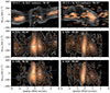 |
Fig. 11. PV diagrams of molecular gas emission along the major (PA = 95°) and minor (PA = 5°) axes of the galaxy. Top row: CO(2–1) emission from GB09 as a color map, with white contours of the H2 S(1) line overlaid. A velocity shift of 30 km s−1 was applied to the CO data to match our systemic velocity. Second and third rows: H2 S(5) and S(9) emission lines, respectively. In all major-axis panels, the blue line marks the best-fit CO rotation curve. Contours begin at 10σ. |
Along the minor axis, the H2 S(5) line displays a broad component centered at -100 km s−1, extending spatially from -200 to +200 pc. At higher excitation (S(9)), the southern lane fades significantly, whereas the northern complex remains bright, suggesting asymmetric energy injection or excitation. While jet signatures are subtle, extended northern emission seen in VLA maps may trace gas entrained in a weak jet-driven outflow. These features could correspond to out-of-plane motions, with de-projected velocities of 120–170 km s−1. The NE complex shows weak associated radio emission but otherwise resembles an in-plane shock, mirrored by the SW structure. Together, they delineate a C-type shock front tracing the boundary of an expanding bubble driven by jet feedback. The morphology seen in the channel maps, combined with the estimated molecular gas masses and the alignment of higher-excitation lines with the disk rotation, all support the interpretation that these structures lie within the galactic disk rather than above or below it. This indicates that the bulk of the shocked gas remains within the disk, even if the jet escapes the galaxy plane. De-projected velocities of the H2 S(1) line in these regions typically reach ∼170 km s−1, while higher-excitation lines such as S(9) extend up to ∼340 km s−1.
Outside the jet axis, double-horned line profiles in the warm H2 emission highlight the disrupted nature of the shock’s leading edge, as shown in Fig. 12. They appear in regions that spatially align with interruptions in the SF ring, where high-excitation H2 transitions coincide with non-UV emission. Spectra in two of these regions within a ∼30 pc aperture reveal two symmetric, narrow velocity components with a separation of ∼100 km s−1, and both showing similarly high excitation levels. Further evidence of stratified feedback emerges from the spatial decoupling between warm H2, Paα, and UV. The UV emission tracing the SF ring lies just outside the warm H2 in the outflowing NE structure, with a similar configuration observed in the SW, where the ring borders the outer edge of the SW shock. This spatial sequence is consistent with a scenario in which mechanical energy injected by the expanding bubble driven by the jet is propelling H2 outflows and displacing large gas masses that compress the ISM, enabling SF to proceed relatively undisturbed in a surrounding ring. Rayleigh–Taylor instabilities may also arise where a low-density shock collides with denser material from the SF ring, likely producing the observed double-horned H2 profiles.
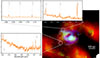 |
Fig. 12. Color composite: H2 S(1) (red), H2 1–0 S(1) (green), and Paα (blue) with UV contours. The spectra show the double-horned profiles of the high excitation H2 lines. |
In the southern part of the SF ring, a partial decoupling of Paα and UV emission suggests that the most massive stars (≳20 M⊙) have already exploded as supernovae and dispersed their surrounding H II regions. The remaining UV could originate from intermediate-mass stars (3–10 M⊙), which emit nonionizing UV radiation for up to ∼30 Myr, implying that the last SF burst ended 8–30 Myr ago. Sub-equilibrium OPR values point to recent shock activity with estimated ages of 0.1–1 Myr (Neufeld et al. 2006). Taken together, the OPR, UV and Paα distributions may trace distinct but complementary timescales. Assuming similar shock velocities, the travel time to 200 pc would be ∼1 Myr, while reaching kiloparsec scales would require ∼10 Myr. This suggests that the kpc-scale cocoon observed by O24 is consistent in age with the last SF burst. In contrast, the warm H2 excitation seen in the NE and SW traces a more recent (∼1 Myr) shock event, likely resulting from ongoing interaction between the jet and the ISM. A full analysis of the ionized gas and the PAH emission will be presented in a forthcoming work to characterize the multiphase interplay and impact on SF.
Overall, LLAGN feedback in M58 does not drive fast winds or expel large gas reservoirs. Instead, it acts subtly, disturbing the inner 200 pc through C-type shocks and turbulence, with warm H2 outflows reaching ∼170 km s−1, while the large-scale rotating disk is just thermally heated. Other observational studies support this scenario. An excess of warm H2 is commonly seen near AGN (Lambrides et al. 2019). In some cases, such as NGC 3100, the jet mildly perturbs the gas kinematics (Ruffa et al. 2022). Broader samples show that, beyond a certain radius, jets typically have minimal dynamical impact on the ISM (Ayubinia et al. 2023; Kukreti et al. 2025). In low-Eddington phases, molecular gas builds up around the nucleus, and only jets aligned with the disk can remove it efficiently (García-Burillo et al. 2024).
Ultimately, M58 illustrates the long-term impact of low-power AGN feedback, primarily driven by an off-plane radio jet and, in second order, by X-ray photons from the ADAF. Rather than clearing the ISM, the AGN regulates it by heating the inner disk via C-type shocks and quenching SF up to kiloparsec scales with non-dynamical coupling. In regions where shocks impact dense gas directly, we observe mildly disturbed kinematics and excitation conditions that resemble the effects of more powerful AGN, albeit on smaller scales. These findings highlight the cumulative impact of sustained, low-level LLAGN feedback in shaping both the ISM structure and the SF potential of galaxies.
6. Summary and conclusions
JWST’s unprecedented sensitivity opens a new window into the subtle but significant impact of LLAGN feedback. In this study, we presented the most detailed near and mid-IR view to date of the inner kiloparsec of M58, revealing the physical conditions, excitation mechanisms, and kinematics of warm H2 in the vicinity of a weak AGN with a low-power radio jet. Our main findings can be summarized as follows:
-
We detect pure bright H2 rotational lines (S(1)–S(18)) across the inner disk, consistent with low-velocity C-type shocks (10–40 km s−1) moving perpendicular to the jet axis. Their excitation diagrams are well described by a power-law temperature distribution with an exponential cutoff (see Eq. (1)).
-
Bright rovibrational H2 lines from the ν = 1 and 2 levels are also detected. Their excitation deviates from thermal expectations mainly due to low densities. Nonthermal processes contribute 10–30% of rovibrational emission, likely powered by an ADAF producing X-ray radiation.
-
The OPRs drop to 1.5–2.5 in shocked regions. These sub-equilibrium values trace recent shocks (∼0.1–1 Myr), before the OPR conversion equilibrates.
-
Jet-driven low-velocity shocks heat the H2 without disturbing the kinematics of large-scale dust lanes. In contrast, the inner ∼200 pc exhibit disturbed kinematics and outflow-like features, consistent with turbulent molecular gas displacement and compression spatially coincident with the edge of the circumnuclear SF ring. Double-horned H2 line profiles at the shock front indicate turbulent, stratified feedback.
These results demonstrate that even low-luminosity AGN can produce sustained and measurable influence on their host galaxies, not by ejecting gas through high-velocity winds, but by subtly reshaping the molecular ISM via turbulence, shocks, and thermal regulation. In M58, this “gentle” feedback thermally perturbs the inner disk and quenches SF at kiloparsec scales, while producing turbulent motions only in the center. M58 thus exemplifies the cumulative, stratified nature of low-power AGN feedback: long-lived and spatially structured, with observable imprints in gas excitation, dynamics, and SF history.
Future studies will be essential to determine how common this scenario is in broader population of LLAGN. Systematic JWST surveys of nearby AGN-hosting galaxies, in combination with high-resolution ALMA and radio data, will be critical for quantifying the frequency, energetics, and long-term impact of weak AGN feedback in the local universe.
See Equations 1 and 2 in Mazzalay et al. (2013).
S(3) contributes ∼35% of the summed S(1)–S(5) luminosity measured by Spitzer over the central 2 kpc.
These were calibrated at 1.4 GHz and 323 MHz; we extrapolated assuming a typical synchrotron spectral index of α = −0.8
Available online at https://github.com/ie-lopez/MPF
Acknowledgments
We thank A. Alonso-Herrero, I. Garcia-Bernete, S. Quai, M. Ceci and L. Ulivi for useful discussion. We also thank M. Dadina for providing access to his computational facilities. IEL acknowledges support from the Cassini Fellowship program at INAF-OAS. EB and GC acknowledge financial support from INAF under the Large Grant 2022 “The metal circle: a new sharp view of the baryon cycle up to Cosmic Dawn with the latest generation IFU facilities” and the GO grant “A JWST/MIRI MIRACLE: Mid-IR Activity of Circumnuclear Line Emission”. EB also acknowledges financial support from “Ricerca Fondamentale 2024” program (mini-grant 1.05.24.07.01). SGB acknowledges support from the Spanish grant PID2022-138560NB-I00, funded by MCIN/AEI/10.13039/501100011033/FEDER, EU. The color schemes used in this work are color-blind friendly from Paul Tol’s Note.
References
- Alatalo, K., Blitz, L., Young, L. M., et al. 2011, ApJ, 735, 88 [NASA ADS] [CrossRef] [Google Scholar]
- Appleton, P. N., Xu, K. C., Reach, W., et al. 2006, ApJ, 639, L51 [NASA ADS] [CrossRef] [Google Scholar]
- Appleton, P. N., Guillard, P., Emonts, B., et al. 2023, ApJ, 951, 104 [NASA ADS] [CrossRef] [Google Scholar]
- Ayubinia, A., Woo, J.-H., Rakshit, S., & Son, D. 2023, ApJ, 954, 27 [NASA ADS] [CrossRef] [Google Scholar]
- Baldi, R. D., Williams, D., McHardy, I., et al. 2018, MNRAS, 476, 3478 [Google Scholar]
- Baldi, R. D., Williams, D., McHardy, I., et al. 2021, MNRAS, 500, 4749 [Google Scholar]
- Balmaverde, B., Capetti, A., Moisio, D., Baldi, R. D., & Marconi, A. 2016, A&A, 586, A48 [NASA ADS] [CrossRef] [EDP Sciences] [Google Scholar]
- Bertola, E., Circosta, C., Ginolfi, M., et al. 2024, A&A, 691, A178 [NASA ADS] [CrossRef] [EDP Sciences] [Google Scholar]
- Bessiere, P. S., & Ramos Almeida, C. 2022, MNRAS, 512, L54 [NASA ADS] [CrossRef] [Google Scholar]
- Black, J. H., & van Dishoeck, E. F. 1987, ApJ, 322, 412 [Google Scholar]
- Boselli, A., Cuillandre, J. C., Fossati, M., et al. 2016, A&A, 587, A68 [NASA ADS] [CrossRef] [EDP Sciences] [Google Scholar]
- Brand, P. W. J. L., Toner, M. P., Geballe, T. R., et al. 1989, MNRAS, 236, 929 [NASA ADS] [CrossRef] [Google Scholar]
- Brusa, M., Cresci, G., Daddi, E., et al. 2018, A&A, 612, A29 [NASA ADS] [CrossRef] [EDP Sciences] [Google Scholar]
- Burke, C. J., Natarajan, P., Baldassare, V. F., & Geha, M. 2025, ApJ, 978, 77 [Google Scholar]
- Bushouse, H., Eisenhamer, J., & Dencheva, N. 2025, https://doi.org/10.5281/zenodo.8145703 [Google Scholar]
- Cappellari, M. 2023, MNRAS, 526, 3273 [NASA ADS] [CrossRef] [Google Scholar]
- Cappellari, M., & Emsellem, E. 2004, PASP, 116, 138 [Google Scholar]
- Cavagnolo, K. W., McNamara, B. R., Nulsen, P. E. J., et al. 2010, ApJ, 720, 1066 [Google Scholar]
- Ceci, M., Cresci, G., Arribas, S., et al. 2025, A&A, 695, A116 [NASA ADS] [CrossRef] [EDP Sciences] [Google Scholar]
- Cicone, C., Maiolino, R., Sturm, E., et al. 2014, A&A, 562, A21 [NASA ADS] [CrossRef] [EDP Sciences] [Google Scholar]
- Comerón, S., Knapen, J., Beckman, J., & Shlosman, I. 2008, A&A, 478, 403 [NASA ADS] [CrossRef] [EDP Sciences] [Google Scholar]
- Draine, B. T., & Bertoldi, F. 1996, ApJ, 468, 269 [Google Scholar]
- Draine, B. T., & Woods, D. T. 1990, ApJ, 363, 464 [NASA ADS] [CrossRef] [Google Scholar]
- Edler, H. W., de Gasperin, F., Shimwell, T. W., et al. 2023, A&A, 676, A24 [NASA ADS] [CrossRef] [EDP Sciences] [Google Scholar]
- Emonts, B. H. C., Piqueras-López, J., Colina, L., et al. 2014, A&A, 572, A40 [EDP Sciences] [Google Scholar]
- Flower, D. R., Pineau Des Forêts, G., & Walmsley, C. M. 2006, A&A, 449, 621 [NASA ADS] [CrossRef] [EDP Sciences] [Google Scholar]
- García-Bernete, I., Rigopoulou, D., Donnan, F. R., et al. 2024, A&A, 691, A162 [NASA ADS] [CrossRef] [EDP Sciences] [Google Scholar]
- García-Burillo, S., Fernández-García, S., Combes, F., et al. 2009, A&A, 496, 85 [NASA ADS] [CrossRef] [EDP Sciences] [Google Scholar]
- García-Burillo, S., Hicks, E., Alonso-Herrero, A., et al. 2024, A&A, 689, A347 [NASA ADS] [CrossRef] [EDP Sciences] [Google Scholar]
- González-Alfonso, E., Fischer, J., Bruderer, S., et al. 2018, ApJ, 857, 66 [Google Scholar]
- Goold, K., Seth, A., Molina, M., et al. 2024, ApJ, 966, 204 [NASA ADS] [CrossRef] [Google Scholar]
- Guillard, P., Boulanger, F., Pineau Des Forêts, G., & Appleton, P. N. 2009, A&A, 502, 515 [NASA ADS] [CrossRef] [EDP Sciences] [Google Scholar]
- Guillard, P., Ogle, P. M., Emonts, B. H. C., et al. 2012, ApJ, 747, 95 [NASA ADS] [CrossRef] [Google Scholar]
- Habart, E., Walmsley, M., Verstraete, L., et al. 2005, Space Sci. Rev., 119, 71 [Google Scholar]
- Harrison, C. M., & Ramos Almeida, C. 2024, Galaxies, 12, 17 [NASA ADS] [CrossRef] [Google Scholar]
- Harrison, C. M., Thomson, A. P., Alexander, D. M., et al. 2015, ApJ, 800, 45 [Google Scholar]
- Heckman, T. M., & Best, P. N. 2014, ARA&A, 52, 589 [Google Scholar]
- Ho, L. C. 2008, ARA&A, 46, 475 [Google Scholar]
- Ho, L. C., & Ulvestad, J. S. 2001, ApJS, 133, 77 [NASA ADS] [CrossRef] [Google Scholar]
- Holdship, J., Mangum, J. G., Viti, S., et al. 2022, ApJ, 931, 89 [NASA ADS] [CrossRef] [Google Scholar]
- Hollenbach, D. J., & Tielens, A. G. 1999, Rev. Mod. Phys., 71, 173 [CrossRef] [Google Scholar]
- Indriolo, N., & McCall, B. J. 2012, ApJ, 745, 91 [NASA ADS] [CrossRef] [Google Scholar]
- Indriolo, N., Neufeld, D. A., Gerin, M., et al. 2015, ApJ, 800, 40 [NASA ADS] [CrossRef] [Google Scholar]
- Jarvis, M. E., Harrison, C. M., Mainieri, V., et al. 2020, MNRAS, 498, 1560 [NASA ADS] [CrossRef] [Google Scholar]
- Kharb, P., & Silpa, S. 2023, Galaxies, 11, 27 [Google Scholar]
- Kristensen, L. E., Godard, B., Guillard, P., Gusdorf, A., & Pineau des Forêts, G. 2023, A&A, 675, A86 [NASA ADS] [CrossRef] [EDP Sciences] [Google Scholar]
- Kukreti, P., Wylezalek, D., Albán, M., & Dall’Agnol de Oliveira, B. 2025, A&A, 698, A99 [NASA ADS] [CrossRef] [EDP Sciences] [Google Scholar]
- Lambrides, E. L., Petric, A. O., Tchernyshyov, K., Zakamska, N. L., & Watts, D. J. 2019, MNRAS, 487, 1823 [Google Scholar]
- Lammers, C., Iyer, K. G., Ibarra-Medel, H., et al. 2023, ApJ, 953, 26 [NASA ADS] [CrossRef] [Google Scholar]
- Law, D. R., Morrison, E. Jr., Argyriou, I., et al. 2023, AJ, 166, 45 [NASA ADS] [CrossRef] [Google Scholar]
- López, I. E., Yang, G., Mountrichas, G., et al. 2024, A&A, 692, A209 [NASA ADS] [CrossRef] [EDP Sciences] [Google Scholar]
- Maoz, D., Nagar, N. M., Falcke, H., & Wilson, A. S. 2005, ApJ, 625, 699 [NASA ADS] [CrossRef] [Google Scholar]
- Marasco, A., Cresci, G., Nardini, E., et al. 2020, A&A, 644, A15 [EDP Sciences] [Google Scholar]
- Maraston, C., & Strömbäck, G. 2011, MNRAS, 418, 2785 [Google Scholar]
- Mazzalay, X., Saglia, R. P., Erwin, P., et al. 2013, MNRAS, 428, 2389 [NASA ADS] [CrossRef] [Google Scholar]
- Mezcua, M., & Prieto, M. A. 2014, ApJ, 787, 62 [NASA ADS] [CrossRef] [Google Scholar]
- Mingo, B., Croston, J. H., Hardcastle, M. J., et al. 2019, MNRAS, 488, 2701 [NASA ADS] [CrossRef] [Google Scholar]
- Morganti, R., Tadhunter, C. N., & Oosterloo, T. A. 2005, A&A, 444, L9 [NASA ADS] [CrossRef] [EDP Sciences] [Google Scholar]
- Mouri, H. 1994, ApJ, 427, 777 [NASA ADS] [CrossRef] [Google Scholar]
- Mukherjee, D., Bicknell, G., Sutherland, R., & Wagner, A. 2016, MNRAS, 461, 967 [NASA ADS] [CrossRef] [Google Scholar]
- Mukherjee, D., Bicknell, G., Wagner, A., Sutherland, R., & Silk, J. 2018, MNRAS, 479, 5544 [NASA ADS] [CrossRef] [Google Scholar]
- Mullaney, J. R., Daddi, E., Béthermin, M., et al. 2012, ApJ, 753, L30 [Google Scholar]
- Nemmen, R., Storchi-Bergmann, T., & Eracleous, M. 2014, MNRAS, 438, 2804 [NASA ADS] [CrossRef] [Google Scholar]
- Neufeld, D. A., & Wolfire, M. G. 2017, ApJ, 845, 163 [Google Scholar]
- Neufeld, D. A., Melnick, G. J., Sonnentrucker, P., et al. 2006, ApJ, 649, 816 [NASA ADS] [CrossRef] [Google Scholar]
- Newville, M. 2023, https://doi.org/10.5281/zenodo.8145703 [Google Scholar]
- Novak, G. S., Ostriker, J. P., & Ciotti, L. 2011, ApJ, 737, 26 [Google Scholar]
- Ogle, P., Antonucci, R., Appleton, P. N., & Whysong, D. 2007, ApJ, 668, 699 [NASA ADS] [CrossRef] [Google Scholar]
- Ogle, P., Boulanger, F., Guillard, P., et al. 2010, ApJ, 724, 1193 [NASA ADS] [CrossRef] [Google Scholar]
- Ogle, P. M., López, I. E., Reynaldi, V., et al. 2024, ApJ, 962, 196 [NASA ADS] [CrossRef] [Google Scholar]
- Otter, J. A., Alatalo, K., Rowlands, K., et al. 2024, ApJ, 975, 142 [Google Scholar]
- Padovani, M., Ivlev, A. V., Galli, D., & Caselli, P. 2018, A&A, 614, A111 [NASA ADS] [CrossRef] [EDP Sciences] [Google Scholar]
- Padovani, M., Bialy, S., Galli, D., et al. 2022, A&A, 658, A189 [NASA ADS] [CrossRef] [EDP Sciences] [Google Scholar]
- Perna, M., Arribas, S., Marshall, M., et al. 2023, A&A, 679, A89 [NASA ADS] [CrossRef] [EDP Sciences] [Google Scholar]
- Pierce, J. C. S., Tadhunter, C. N., & Morganti, R. 2020, MNRAS, 494, 2053 [NASA ADS] [CrossRef] [Google Scholar]
- Ramos Almeida, C., Acosta-Pulido, J., Tadhunter, C., et al. 2019, MNRAS, 487, L18 [NASA ADS] [CrossRef] [Google Scholar]
- Reeves, R. R., & Harteck, P. 1979, Zeitschrift Naturforschung Teil A, 34, 163 [Google Scholar]
- Riffel, R., Rodríguez-Ardila, A., Aleman, I., et al. 2013, MNRAS, 430, 2002 [NASA ADS] [CrossRef] [Google Scholar]
- Rodríguez-Ardila, A., Pastoriza, M., Viegas, S., Sigut, T., & Pradhan, A. 2004, A&A, 425, 457 [NASA ADS] [CrossRef] [EDP Sciences] [Google Scholar]
- Roueff, E., Abgrall, H., Czachorowski, P., et al. 2019, A&A, 630, A58 [NASA ADS] [CrossRef] [EDP Sciences] [Google Scholar]
- Roussel, H., Helou, G., Hollenbach, D. J., et al. 2007, ApJ, 669, 959 [NASA ADS] [CrossRef] [Google Scholar]
- Ruffa, I., Prandoni, I., Davis, T. A., et al. 2022, MNRAS, 510, 4485 [NASA ADS] [CrossRef] [Google Scholar]
- Ruiz-Lapuente, P. 1996, ApJ, 465, L83 [Google Scholar]
- Rupke, D. S. N., & Veilleux, S. 2013, ApJ, 775, L15 [NASA ADS] [CrossRef] [Google Scholar]
- Sabater, J., Best, P. N., Hardcastle, M. J., et al. 2019, A&A, 622, A17 [NASA ADS] [CrossRef] [EDP Sciences] [Google Scholar]
- Shin, J., Woo, J.-H., Chung, A., et al. 2019, ApJ, 881, 147 [Google Scholar]
- Smith, J. D. T., Draine, B. T., Dale, D. A., et al. 2007, ApJ, 656, 770 [Google Scholar]
- Somerville, R. S., & Davé, R. 2015, ARA&A, 53, 51 [Google Scholar]
- Spindler, R. 1969, J. Quant. Spectr. Rad. Transf., 9, 1041 [Google Scholar]
- Sternberg, A. 1989, ApJ, 347, 863 [NASA ADS] [CrossRef] [Google Scholar]
- Sternberg, A., Le Petit, F., Roueff, E., & Le Bourlot, J. 2014, ApJ, 790, 10 [CrossRef] [Google Scholar]
- Storchi-Bergmann, T., McGregor, P., Riffel, R., et al. 2009, MNRAS, 394, 1148 [NASA ADS] [CrossRef] [Google Scholar]
- Togi, A., & Smith, J. D. T. 2016, ApJ, 830, 18 [NASA ADS] [CrossRef] [Google Scholar]
- Tozzi, G., Cresci, G., Marasco, A., et al. 2021, A&A, 648, A99 [NASA ADS] [CrossRef] [EDP Sciences] [Google Scholar]
- Ulivi, L., Venturi, G., Cresci, G., et al. 2024, A&A, 685, A122 [NASA ADS] [CrossRef] [EDP Sciences] [Google Scholar]
- Ulivi, L., Perna, M., Lamperti, I., et al. 2025, A&A, 693, A36 [NASA ADS] [CrossRef] [EDP Sciences] [Google Scholar]
- Van De Putte, D., Meshaka, R., Trahin, B., et al. 2024, A&A, 687, A86 [NASA ADS] [CrossRef] [EDP Sciences] [Google Scholar]
- Vleugels, C., McClure, M., Sturm, A., & Vlasblom, M. 2025, A&A, 695, A145 [NASA ADS] [CrossRef] [EDP Sciences] [Google Scholar]
- Wakelam, V., Bron, E., Cazaux, S., et al. 2017, Mol. Astrophys., 9, 1 [Google Scholar]
- Webster, B., Croston, J. H., Mingo, B., et al. 2021, MNRAS, 500, 4921 [Google Scholar]
- Wilgenbus, D., Cabrit, S., Pineau des Forêts, G., & Flower, D. R. 2000, A&A, 356, 1010 [NASA ADS] [Google Scholar]
- Yuan, F., & Narayan, R. 2014, ARA&A, 52, 529 [NASA ADS] [CrossRef] [Google Scholar]
- Zanchettin, M., Ramos Almeida, C., Audibert, A., et al. 2025, A&A, 695, A185 [NASA ADS] [CrossRef] [EDP Sciences] [Google Scholar]
Appendix A: Data reduction
Data were reduced using the JWST Science Calibration Pipeline (Bushouse et al. 2025). For NIRCam and MIRI, we used version 1.17.1 with CRDS context jwst1321.pmap. The NIRSpec data was processed with the JWST calibration pipeline version 1.15.1 using the CRDS context jwst1303.pmap. Processing parameters were tailored to each observing mode, with additional custom routines described below.
For imaging modes, we used the suppressonegroup= False option during ramp fitting to recover partially saturated pixels using frame0 exposures. Backgrounds were subtracted via sigma-clipped medians measured in off-source regions. NIRCam 1/f noise was suppressed using Cleanflickernoise from the det1dict module, applied across all channels.
Astrometric alignment was performed using NIRCam as reference frame, given its superior positional accuracy among the JWST instruments used. The NIRSpec H2 1–0 S(1) line map was aligned to the NIRCam F212N image, yielding offsets of δRA = 0 15 and δDec = 0
 13. For MIRI, the H2 S(8) line was aligned to the NIRSpec corrected frame, with offsets of δRA = 0
 05 and δDec = –0
 08. Final cubes were resampled using the EMSM algorithm to a spatial scale of ∼0
 1.
1.
NIRSpec data were reduced with custom outlier rejection scripts to mitigate residual cosmic rays. We corrected for the artifacts from spatial under-sampling of the PSF, also known as "wiggles," using the algorithm by Perna et al. (2023). This tool was applied only within a ∼5-pixel radius centered on the AGN, where the effect is significant due to source brightness.
MIRI MRS data required extensive correction to address fringing and noise resampling artifacts. Fringing was removed using a dedicated 2D correction algorithm. In Channels 3 and 4, fringing correction was deactivated due to the absence of significant interference patterns. A custom correction was necessary for noise resampling, particularly in Channel 1, where the dither strategy under-sampled the PSF, producing artificial flux jumps near the central AGN.
Using a similar idea behind the "wiggles” algorithm, for each problematic MIRI MRS spaxel s(λ), a reference spectrum sref(λ) was extracted by averaging the spectra within a circular 5-pixel aperture centered around the spaxel. Both the spaxel and reference spectra were processed to isolate the continuum emission by masking emission lines and PAH features. The masked regions were interpolated, and a Savitzky–Golay filter of the problematic spaxel and its reference spectrum was applied to derive smooth continuum estimates c(λ) and cref(λ) respectively.
The corrected spaxel spectrum scorrected(λ) was then calculated using the following formula:
 (A.1)
(A.1)
This transformation scales the continuum of the spaxel to match that of the local reference while preserving the relative line strengths and spectral shape. A residual 1D fringe correction, derived from the JWST pipeline, was applied to mitigate remaining low-level fringing patterns. An example of this correction process is shown in Figure A.1, where the original and corrected spectra are compared alongside the estimated continuum shapes.
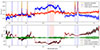 |
Fig. A.1. Example of the spaxel correction method. Top panel: Original spaxel spectrum (blue), its reference continuum (orange), and corrected spectrum (red). Bottom panel: Correction factor for each wavelength and the fringing pattern derived from the JWST pipeline. Masking lines and PAH features are shown in the shaded-blue and shaded-red areas, respectively. |
Some MIRI spaxels exhibited artifacts that mimicked emission lines near the hydrogen recombination lines of the Humphreys series (i.e., HI 7–6). These features were discarded for two main reasons: first, the lines did not exhibit a Gaussian profile consistent with genuine emission; and second, there was no corresponding Pfund-alpha line detected, which should be brighter than HI 7–6 if the signal were real.
MERLIN archival data were obtained from two observations in the C band (centered at 5,GHz, bandwidth 16,MHz) on 14 November and 4 December 2002. The total exposure times were 2.6 and 10.5 hours, respectively. The data were processed using the standard MERLIN pipeline, which includes flagging of bad visibilities, and calibration in both phase and amplitude. The two visibility datasets were combined using the dbcon task in AIPS. Imaging was performed with DIFMAP, using a pixel scale (cell size) of 10 mas. After several iterations of phase self-calibration followed by one iteration of amplitude self-calibration, we achieved a final image with an rms noise level of 0.19 mJy beam−1.
The VLA C-band data were taken in B configuration on 30 June 2020 (Project ID 20A-272, PI: Ogle), with a total bandwidth of 2,GHz, divided into 32 spectral windows each with 64×1 MHz channels. The raw data were calibrated using the standard VLA pipeline within CASA (version 5.3.1). Imaging was carried out with the tclean task using Briggs weighting with robust = 0.5. The resulting synthesized beam was 0 96 × 0
 83, and the rms noise was 24.4 μJy beam−1.
Appendix B: Spectral fitting
For the NIRSpec data, we adopted a multicomponent spaxel-by-spaxel fitting approach following Marasco et al. (2020), Tozzi et al. (2021) with JWST-specific updates from Ceci et al. (2025), Ulivi et al. (2025). The stellar continuum and emission lines were fit simultaneously using the penalized PiXel-Fitting package (pPXF; Cappellari & Emsellem 2004; Cappellari 2023). We modeled the continuum using the single stellar population templates of Maraston & Strömbäck (2011) (R ≃ 20, 000 covering part of Band 2). For λ > 2.5 μm, we used an eighth-order polynomial to approximate the redder continuum shape. Emission lines were modeled with one to three Gaussian components with linked kinematics, selected via a Kolmogorov–Smirnov (KS) test on residuals. The continuum-subtracted cubes were smoothed with a Gaussian kernel of σ = 1 pixel to improve S/N and reduce outliers, at the expense of a slight loss in spatial resolution.
For MIRI MRS, we adapted the method of O244, originally developed for Spitzer IRS, to the higher spatial and spectral resolution of JWST. Fits were performed with the lmfit Python package (Newville 2023), which uses Levenberg–Marquardt least-squares optimization. After masking emission lines, we fit the continuum in each spaxel with a combination of dust continuum, PAH features (modeled with templates similar to PAHFIT; Smith et al. 2007), and a power-law component. We then fit the residual spectra to model emission lines with one to three Gaussians, following a similar approach used for NIRSpec. We further validated the multicomponent selection with the Bayesian and Akaike Information Criteria, which yielded consistent results. The instrumental point spread function (PSF) was not explicitly accounted for during spaxel-by-spaxel fitting; however, for analyses spanning a wide wavelength range, such as excitation diagrams and the flux measurements reported in Table C.1, the NIRSpec and MIRI datacubes were smoothed to match the worst PSF at the H2 S(1) line (FWHM = 0 67), following the wavelength-dependent PSF characterization for MRS by Law et al. (2023). In addition, we chose apertures larger than the PSF, ensuring that PSF-related effects are minimized in the derived fluxes and line ratios. For analyses involving ratios of lines at similar wavelengths, such as the rovibrational line ratios shown in Fig. 9 and discussed in Section 4.5.2, fluxes are measured within the apertures without smoothing. This approach is more accurate because these lines are observed with the same instrument, so PSF mismatches are negligible and only contribute to slightly larger uncertainties.
We verified that both methods yield consistent results for lines covered by both instruments, such as the H2 S(8) transition. Given the superior sensitivity and resolution of NIRSpec, we adopt its measurement for this line. Finally, all integrated spectra were extracted directly from the original cubes, without applying "wiggles" correction, to avoid interpolation artifacts. When integrating over apertures larger than the PSF, the wiggles average out and become negligible. These integrated spectra were modeled using the same spaxel-by-spaxel fitting procedure.
Appendix C: H2 detected lines
Table C.1 lists the H2 emission lines detected in each of the selected regions indicated in Fig. C.1. All reported fluxes are above the 3σ significance threshold. The central AGN region is defined by a 0.5 radius aperture centered on the MERLIN radio core (RA = 189.4313, Dec = 11.8182), encompassing the compact AGN and matched to the MIRI MRS PSF. Four additional circular apertures of 0.3
 radius sample distinct morphological and kinematic features: NE shock (RA = 189.4316, Dec = 11.8184), North Lane (RA = 189.4305, Dec = 11.8185), and South Lane (RA = 189.4323, Dec = 11.8177).
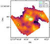 |
Fig. C.1. H2 S(5) line map with selected extraction regions. The central aperture (cyan) is slightly enlarged to match the PSF, while the surrounding apertures sample the NE shock lobe and dust lanes. |
Molecular hydrogen lines detected.
All Tables
All Figures
|
Fig. 1. Left: Composite image showing F200W (blue; stellar continuum), continuum-subtracted H2 1– S(1) from F212N (green), and F770W (red; tracing PAH 7.7 μm emission). The LOFAR 144 MHz radio contours are overlaid. The NIRSpec and MIRI Channel 4 fields of view are shown with cyan and yellow dashed lines, respectively. Right: Zoom-in highlighting warm molecular gas traced by H2 S(9) (green), S(1) (red), and CO 2-1 (blue). Overlaid contours are C band from VLA (white) and MERLIN (black). Key regions are labeled, including the northern and southern dust lanes as well as shocked regions to the northeast and southwest. Physical scale bars are shown in both panels. |
| In the text | |
|
Fig. 2. JWST spectra for the nucleus (blue) and for a circumnuclear region (red). Ionic emission lines are indicated by vertical blue lines. The PAH features and H2 lines are marked along the bottom of each panel. The circumnuclear region exhibits strong PAH emission, pure rotational H2, and low-excitation ionized lines. In contrast, the nuclear spectrum shows prominent high-ionization lines, relatively stronger H2 rovibrational lines, and two silicate features at 10 μm and 17 μm. Shaded-gray regions indicate gaps in the NIRSpec instrument. |
| In the text | |
|
Fig. 3. Moment maps showing H2, low-ionization [Ar II], and high-ionization lines [Ne V]. Only pixels with detections above 5σ are shown. The dashed and dotted gray lines indicate the jet axis and the galaxy’s major axis, respectively. A black x marker indicates the AGN radio core. |
| In the text | |
|
Fig. 4. NIRSpec channel maps, illustrating both rotational and rovibrational kinematics. Top row: H2 1–0 S(1); Bottom row: H2 S(9). Each column corresponds to a velocity bin (from –500 to +500 km s−1). A dashed white line represents the jet axis. Both transitions trace the dust lanes between –300 to +200 km s−1, compatible with rotation. The NE feature, strongest at –500 km s−1 and persisting to +200 km s−1, is identified as the forward shock front. The overall lack of alignment with the jet axis suggests the jet passes outside the disk plane. |
| In the text | |
|
Fig. 5. Maps of pure H2 rotational line ratios. Top: S(3)/S(1) show elevated values in the dust lanes and in two-lobed structures near the AGN. White contours represent the OPR; the outermost contour corresponds to 3 (expected in LTE at T ≳ 200 K), with inner contours decreasing in steps of 0.25 down to 1.5. Middle: S(9)/S(5). Bottom: S(13)/S(7). These ratios reveal that the higher-J lines trace arc-like structures in both lobes. The dashed gray line indicates the jet axis. |
| In the text | |
|
Fig. 6. Predicted pure H2 rotational line ratios as a function of shock velocity, based on the C-type shock models of Kristensen et al. (2023). Two model sets are shown with a magnetic field strength of B = 30 μG and pre-shock densities of nH = 100 cm−3 (solid lines) and nH = 1000 cm−3 (dashed lines). Colored curves indicate different strengths of the external UV radiation field G0. Shaded regions mark the range of observed ratios. Constraints on S(13)/S(7) are similar to those for S(9)/S(5). |
| In the text | |
|
Fig. 7. Maps from the modified power-law temperature distribution model from Togi & Smith (2016). Left: Power-law index n, with lower values indicating a stronger contribution from hotter gas. Center: Lower temperature Tl, contributing to H2 emission. Right: Warm H2 mass per pixel, with each pixel area being ≈161 pc2. White contours trace CO(2–1) emission from cooler molecular gas. The dashed gray line marks the jet axis. |
| In the text | |
|
Fig. 8. H2 excitation ladders for selected regions. Top: Nucleus. Middle: Northeast shock. Bottom: South lane. Pure rotational H2 lines are shown in blue, with best-fit models in yellow triangles. Observed rovibrational lines are plotted in red, with zoomed-in insets displayed in the top corners of each panel. The solid line connects the 1–0 S(1–7) rovibrational ladder, while the dashed line connects the 1–0 O(2–9) ladder. |
| In the text | |
|
Fig. 9. H2 2–1 S(1)/1–0 S(1) vs. 1–0 S(2)/1–0 S(0) emission-line ratios for selected regions of M58. Colored markers indicate the nucleus (Nuc), north and south lane (NL-SL), and the northeast and southwest H2 lobes (NE-SW). The solid black curve marks the predicted trend for pure thermal excitation. Shaded regions represent the domains of alternative excitation mechanisms: UV thermal excitation (Sternberg 1989), X-ray heating (Draine & Woods 1990), shocks (Kristensen et al. 2023), and nonthermal UV fluorescence (Black & van Dishoeck 1987). The gray curve shows mixed thermal and fluorescent excitation models, decreasing from 90% thermal (left) in 10% steps. The top and right axes indicate the vibrational and rotational temperatures (Tvib, Trot) respectively. |
| In the text | |
|
Fig. 10. Radial profile of H2 luminosity surface density compared to various energy input mechanisms. Spitzer IRS and JWST MIRI H2 S(3) measurements are scaled to match the total S(1)–S(5) luminosity. The JWST-derived surface density drops beyond 0.5 kpc due to the limited field of view. Energy surface densities, assuming an overall coupling efficiency of η = 5%, are shown for X-ray radiation pressure and kinetic power from cloud–cloud collisions and from the radio jet. |
| In the text | |
|
Fig. 11. PV diagrams of molecular gas emission along the major (PA = 95°) and minor (PA = 5°) axes of the galaxy. Top row: CO(2–1) emission from GB09 as a color map, with white contours of the H2 S(1) line overlaid. A velocity shift of 30 km s−1 was applied to the CO data to match our systemic velocity. Second and third rows: H2 S(5) and S(9) emission lines, respectively. In all major-axis panels, the blue line marks the best-fit CO rotation curve. Contours begin at 10σ. |
| In the text | |
|
Fig. 12. Color composite: H2 S(1) (red), H2 1–0 S(1) (green), and Paα (blue) with UV contours. The spectra show the double-horned profiles of the high excitation H2 lines. |
| In the text | |
|
Fig. A.1. Example of the spaxel correction method. Top panel: Original spaxel spectrum (blue), its reference continuum (orange), and corrected spectrum (red). Bottom panel: Correction factor for each wavelength and the fringing pattern derived from the JWST pipeline. Masking lines and PAH features are shown in the shaded-blue and shaded-red areas, respectively. |
| In the text | |
|
Fig. C.1. H2 S(5) line map with selected extraction regions. The central aperture (cyan) is slightly enlarged to match the PSF, while the surrounding apertures sample the NE shock lobe and dust lanes. |
| In the text | |
Current usage metrics show cumulative count of Article Views (full-text article views including HTML views, PDF and ePub downloads, according to the available data) and Abstracts Views on Vision4Press platform.
Data correspond to usage on the plateform after 2015. The current usage metrics is available 48-96 hours after online publication and is updated daily on week days.
Initial download of the metrics may take a while.