© The Authors 2026

1 Introduction

Space-borne missions have gathered comprehensive observations from mid-infrared (MIR) to far-infrared (FIR) wavelengths and even to the radio regime. These include both all-sky observations, such as in the WISE (3−22 μm; Wright et al. 2010), AKARI (2−160 μm; Murakami et al. 2007), and Planck (λ ≥ 350 μm; Tauber et al. 2010) surveys, as well as more targeted observations with the Spitzer (λ=3.6−160 μm; Werner et al. 2004), and Herschel (λ=70−500 μm; Pilbratt et al. 2010) satellites. These provide a good starting point for investigations of dust evolution in star-forming clouds. The MIR and FIR parts of the spectrum trace the thermal dust emission but from different components of the overall dust populations. The FIR spectrum is produced by large grains that are mostly in radiative equilibrium with the local radiation field. In contrast, the MIR emission comes from stochastically heated smaller grains and is therefore more sensitive to the lower end of the dust size distribution and the thermal properties of those grains.

Studies of FIR thermal dust emission have revealed variations in the large-grain properties over the whole sky (Planck Collaboration XI 2014), especially within the transitions from atomic to molecular clouds and further to the dense clumps that are more immediately connected to the present star formation in the Galaxy (Lagache et al. 1998; Flagey et al. 2009; Cambrésy et al. 2001; Stepnik et al. 2003; Roy et al. 2013). The dust opacity spectral index β and the absolute value of the opacity itself, κ, vary spatially and as a function of wavelength. The first evidence of this evolution came from balloon-borne FIR and millimetre wavelength observations (Bernard et al. 1999; Dupac et al. 2003; Désert et al. 2008; Paradis et al. 2009; Martin et al. 2012), and the variations have been studied in more detail with satellite data, especially with Herschel and Planck (Paradis et al. 2010; Planck Collaboration XI 2014; Planck Collaboration Int. XXII 2015). The results indicate that the dust FIR spectrum may become steeper (with higher β) and the dust opacity may increase towards dense clumps and cores (Stepnik et al. 2003; Juvela et al. 2015b,a; Scibelli et al. 2023), while the spectrum generally flattens towards longer millimetre wavelengths (Reach et al. 1995; Planck Collaboration XVII 2011; Planck Collaboration XIX 2011; Planck Collaboration Int. XXIX 2016; Paradis et al. 2012). These results indicate changes in both the sizes and optical properties of the grains. Ground-based instruments contribute to the studies with observations of higher angular resolution, probing the internal structure of starless and protostellar cores in the nearby clouds. On the other hand, the elimination of atmospheric effects leads to limited sensitivity to extended emission (e.g. Bianchi et al. 2003; Sadavoy et al. 2013; Bracco et al. 2017; Juvela et al. 2018), which complicates the combination of spaceborne and ground-based observations (e.g. Schuller et al. 2021; Mannfors et al. 2025).

The observational constraints on the dust evolution are stronger if the FIR observations of dust emission are complemented with data from shorter wavelengths. When a high column density cloud is seen against a bright background, it may be possible to use mid-infrared (MIR) absorptions to map the cloud structure. This is the case for massive infrared dark clouds (IRDCs) that are observed against the brighter Galactic disk (Simon et al. 2006; Butler & Tan 2012; Kainulainen & Tan 2013). The method requires measurements (or estimates) of the absolute surface brightness of the background sky and, depending on the wavelength, may have additional uncertainty due to variations in the local heating (e.g. embedded protostars) and potential contribution from light scattering (Juvela & Mannfors 2023).

The NIR extinction is measured more commonly using background point sources. If embedded sources are few or can be excluded, the method is insensitive to local heating and thus applicable even in active star-forming regions. The NIR reddening of stars (e.g. measured with ground-based observations in the J, H, and Ks bands) can be converted to a continuous extinction map with methods such as NICER (Lombardi & Alves 2001) and NICEST (Lombardi 2009). These combine the measured colour excesses and smooth the evidence provided by the individual stars, typically down to a resolution of some arcminutes. The resolution is limited mainly by the number density of the background sources. Apart from the intrinsic colours of the stars (typically estimated using a nearby extinction-free reference field), the extinction estimates depend only on the assumed shape of the NIR extinction curve. The extinction curve is not constant, but has shown relatively little variation between clouds of different density (Indebetouw et al. 2005; Wang & Jiang 2014). In contrast, the FIR to NIR dust opacity ratio has been observed to increase by a factor of a few from diffuse clouds to dense clumps. This is clear evidence of dust evolution and is thus mainly attributed to the increase in FIR dust opacity (Martin et al. 2012; Roy et al. 2013; Ysard et al. 2013; Juvela et al. 2015b, 2020; Juvela 2024).

The interpretation of the FIR data in dense clouds is complicated by the strong temperature gradients that exist between the warm surface layers and the colder interiors of dense filaments and starless cores. One way to take these temperature variations into account, at least approximately, is to use threedimensional radiative transfer (RT) modelling, where the dust temperatures follow self-consistently from the assumptions of the density field, the dust properties, and the radiation sources. Modelling can still have significant uncertainties due to the degeneracies between these factors, especially because the LOS cloud structure and the local radiation field spectra are not directly constrained by observations (Juvela 2024). Models have often concentrated on the combination of FIR emission and NIR extinction (e.g. Stepnik et al. 2003; Ysard et al. 2013; Juvela et al. 2015b), because sensitive measurements of MIR surface brightness are more rare. The light scattering would also provide more information on the grain properties, but is mostly useful when the model geometry is simple and the intensity of the scattered signal has not yet saturated (i.e. for optical depths τ(λ)<1). The NIR scattering (the so-called cloudshine) has been used in only a few cases (Juvela et al. 2012; Saajasto et al. 2021; Juvela et al. 2020), but the MIR scattering (the so-called coreshine) has been investigated for a larger sample of dense cores imaged with Spitzer (e.g. Steinacker et al. 2010; Pagani et al. 2010; Andersen et al. 2014; Steinacker et al. 2015; Lefèvre et al. 2016).

In this paper, we use NIR extinction and FIR dust emission to study dust properties in the Orion Molecular Cloud 3 (OMC-3). Orion is an interesting target as the nearest example of a high-mass star-forming region, with a distance of ∼ 400 pc (Großschedl et al. 2018). In OMC-3 the main structure is a massive filament, part of the northern end of the Orion integralshaped filament (Kainulainen et al. 2017; Hacar et al. 2018; Schuller et al. 2021). OMC-3 thus provides an important point of comparison for previously studied filamentary low-mass starforming clouds and the more massive and more distant IRDCs. Compared to other parts of the OMC, the star-formation activity is still relatively low in OMC-3. This simplifies the modelling, since, at least for the central part of the field, dust is mainly heated by the external radiation field. We concentrate on the modelling of the FIR large-grain emission, using the extinction measurements afterwards to test the accuracy of the model predictions at NIR wavelengths. We test alternative dust models to see which of them are compatible with the OMC-3 observations. The complete modelling of MIR-FIR observations is deferred to a future paper in which we will address the partly separate questions of small-grain emission, MIR absorption, and NIR-MIR scattering.

The contents of the paper are the following. We present the observational data in Sect. 2. The three-dimensional RT modelling methods and the dust models employed are discussed in Sect. 3, and the results of the optimised RT models are presented in Sect. 4. We discuss the results in Sect. 5, before listing our final conclusions in Sect. 6.

2 Observational data

2.1 Observations of extended emission

The Orion Molecular Cloud 3 was mapped with the Herschel telescope as part of the Gould Belt Survey (PI Ph. Andre; André et al. 2010). The 250 μm, 350 μm, and 500 μm observations with the SPIRE instrument were done in parallel mode (observation IDs 1342218967 and 1342218968), together with 70 μm and 160 μm observations with the PACS instrument. The relative calibration accuracy of the SPIRE observations is expected to be better than 2%¹, and for the PACS data we assume 4% uncertainty relative to SPIRE.

The resolution of the SPIRE observations is about 18, 26, and 37 arcsec, at 250 μm, 350 μm, and 500 μm, respectively. For the modelling, the maps were degraded to lower resolution using the convolution kernels of Aniano et al. (2011), with the final resolution corresponding to Gaussian beams with FWHM values of 30^′′, 30^′′, and 41^′′, respectively. The size of the map pixels was set to 4^′′, which also corresponds to the spatial discretisation of the three-dimensional models (Sect. 3.2). The nominal resolution of the fitted models was 30^′′ (as described in Sect. 3), and the PACS 70 μm and 160 μm maps were thus also convolved to this resolution. The lower spatial resolution decreased the run times of the model optimisation, with only minor loss of information. The 500 μm band remains important for constraining the spectral index (and therefore also the temperatures) and was used near the original resolution.

2.1.1 Colour corrections

To simplify the comparison with models, observed surface brightness maps were colour corrected to monochromatic values at the nominal wavelengths. For the SPIRE data, the correction was based on modified black-body (MBB) spectra, I_v ∝ B_ν(T) × ν^β, where the temperatures were obtained from MBB fits to the SPIRE data at 41“ angular resolution. The fits used a constant dust opacity spectral index of β=1.8 (cf. Sect. 3.1) and took into account colour corrections in the fits. The SPIRE colour corrections are only a couple of per cent and also change slowly as functions of temperature and spectral index. The PACS 160 μm data were colour corrected for the same MBB spectra. We do not use the 70 μm data in this paper, because these can already have a significant contribution from stochastically heated grains.

2.1.2 Background subtraction

The initial modelling relied on the SPIRE surface brightness data. In the Herschel Science Archive², the zero points of the SPIRE intensity scales have already been adjusted by comparing the maps with Planck absolute surface brightness measurements. However, the RT models represent only part of the OMC-3 cloud, also in the LOS direction, and one has to subtract from the maps the extended emission that is thought to originate outside this volume. Background subtraction was done by subtracting the mean value under a FWHM = 1^′ Gaussian beam that was placed at the first reference position of RA = 5:34:46.1 and Dec = −5:01:59.3 (J2000). In the following, I_v refers to these background-subtracted intensities.

The first reference position is outside the area covered by PACS observations (Fig. 1). Therefore, we used a second reference position at RA =5: 34: 59.3 and Dec =−5: 01: 41.9(J 2000) that is located inside the PACS maps. The PACS zero point was adjusted so that in this position the corrected PACS map matches the extrapolation from the already background-subtracted SPIRE data. The extrapolation was done using an MBB spectrum that was fitted to the SPIRE bands, and for the comparison the surface brightness values were averaged over a 1^′ beam. At the second reference position, the 160 μm surface brightness is less than ∼ 10% of the values in the main filament. The error in the procedure used to set the PACS zero level is a fraction of this number (e.g. 1 K error in temperature plus 0.2 unit error in β would result in a less than 20% error in the extrapolation and thus would have less than 2% effect on the final values in the filament). Therefore, we assume that the 4% relative calibration uncertainty of PACS data also covers the PACS zero point uncertainty in the main filament (relative to SPIRE). Figure 1 shows the final background-subtracted maps at 160, 250, and 500 μm. The figure also shows for reference the 70 μm map, which, however, is not used in the subsequent analysis.

2.2 Cloud masks

We used infrared maps to create a mask that was used in the model optimisation and in the comparison of the model predictions and observations. The mask has six levels, as shown in Fig. 2. The value Q=−1 corresponds to regions where the background-subtracted FIR surface brightness is close to zero or negative (I_ν(350 μm)<1 MJysr⁻¹) and are excluded from the analysis. The values Q=0−2 correspond, respectively, to regions that we refer to as the diffuse background (1 MJysr⁻¹<I_v(350 μm)<190 MJysr⁻¹), the filament region (190 MJy sr⁻¹<I_v(350 μm)<600 MJy sr⁻¹), and the ridge regions (600 MJy sr⁻¹<I_ν(350 μm)<2500 MJy sr⁻¹). We further separated the brightest regions of the ridge as Q=3 (I_v(350 μm)>2500 MJysr⁻¹) where the modelling could be unreliable due to potential unresolved internal radiation sources.

The value Q=4 is reserved for resolved FIR point sources (masked by hand), but also excludes the southern and northern ends of the filament, where the surface brightness increases due to embedded sources and luminous stars outside the map. These cuts are made along lines of constant declination, which correspond roughly to the contour T_dust=25 K from the MBB temperature map. However, the mask is more conservative, excluding all regions far from the field centre. It excludes especially the southern parts, where high column densities make the temperatures low in spite of the increasing strength of the external radiation. Strong MIR point sources were masked by hand and given a mask value of Q=5, even when there is no direct evidence that these sources affect FIR emission at the 30^′′ scale. All regions with Q ≥ 3 were excluded from the analysis.

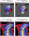Fig. 1 Examples of OMC-3 observations. The maps show background-subtracted surface brightness values (non-linear colour scale) smoothed to the resolution used in the model fits. The plotted area is identical to previous figures. Frame c shows the outline of the PACS coverage and the reference areas for the SPIRE background subtraction (larger white circle) and for the adjustment of the PACS zero level (smaller white circle).

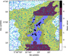Fig. 2 Masks for the OMC-3 field. The levels correspond to areas with low emission (Q=−1), extended cloud (Q=0), filament (Q=1), ridge (Q=2), bright parts of the ridge (Q=3), FIR point sources and highsurface brightness areas affected by local heating (Q=4), and MIR point sources (Q=5). The small dots correspond to the NIR star-like (cyan) and potentially extended (blue) sources that are the basis of the NIR extinction map (Meingast et al. 2016).

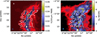Fig. 3 Comparison of τ(250 μm) optical depth map derived from Herschel observations at 41′′ resolution (frame a) and NICER extinction map of Meingast et al. (2016) at 1’ resolution (frame b). The white and grey contours show, respectively, the outlines of the filament (Q=1) and the ridge (Q=2) regions. The black contours separate other high column density areas that are excluded from the analysis (Q>2).

2.3 NIR extinction

We used the J, H, and K_S band NIR observations from the Vienna survey in Orion (VISION; Meingast et al. 2016) and also their NIR extinction map, made using the NICER method (Lombardi & Alves 2001), and the Indebetouw et al. (2005) extinction curve. The map has an angular resolution of FWHM=1^′ beam.

Figure 3 shows a map of the 250 μm optical depth (estimated from Herschel data at 41“ resolution, cf. Sect. 3.1) and the NICER extinction map from Meingast et al. (2016). The original NICER map was resampled to equatorial coordinates using smaller pixels and no interpolation, retaining the original nominal ∼ 1^′ resolution. Although the filament region is clearly visible on both maps, the NICER map shows less correlation with the regions of highest Herschel column densities (e.g. along the Q=2 ridge).

The area of Fig. 2 contains 3141 sources detected in all three NIR bands. These can even be used as individual probes of the extinction, with much greater statistical uncertainty but without the bias introduced by the spatial averaging of the data that show gradients in the stellar number density. The density of background stars decreases from the diffuse background (1126 sources in the Q=0 area) to the filament (Q=1 with 210 sources) and further to the ridge (Q=2 with 70 sources). In the ridge the sampling is also non-uniform and the probability for embedded and foreground sources increases. After subtracting the average extinction in the Q=0 area (for the individual stars and the NICER map separately) and rejecting the individual stars with negative extinction (extinction below the average in the Q=0 area, such as possible foreground sources), the median ratio between the extinction of the individual stars and the NICER values, read at the same positions, is 0.95 in the Q = 1 and 1.14 in the Q = 2 area. The NICER map could be biased towards the ridge, when stars are detected preferentially towards the lower column density part of each resolution element. However, comparison with the median value of individual stars in the Q=2 area shows a difference of less than ∼ 10%. The bias could be larger close to the unresolved density peaks, but these fall mainly inside the already excluded Q > 2 mask (Fig. 2). We used the NICER A(J) extinction map for visual inspection (Fig. 3b, 1’ resolution). When the extinction of an RT model was compared to observations (and especially when estimates needed to be recalculated for the extinction curve of the dust model in question), we used the median A(J) of the individual stars inside a given mask region. For consistency with modelling that used background-subtracted FIR maps and to take into account the lower resolution and the large relative noise of the extinction estimates, background subtraction was done by subtracting the median extinction in the Q=−1 area. That includes the SPIRE reference position and, based on Fig. 3, already has an average extinction close to zero.

3 Methods

The RT modelling started with the definition of the initial threedimensional density field, the radiation sources, and the dust model. The column densities and the strength of the radiation sources were then modified iteratively to provide the best match to the FIR data. The fit procedure was similar to that used in Juvela (2024).

3.1 Modified black-body fits

MBB fits were used to initialise the column densities of the cloud models. Assuming a single dust temperature along the full LOS and optically thin emission, the dust (colour) temperature T_d was obtained by fitting multi-frequency observations with $$I_v\propto B_v\left(T_{\mathrm{d}}\right)\times v^{\beta },$$(1) with Planck law B_v. The optical depth at a given frequency v is then $${\tau }_v=I_v/B_v\left(T_{\mathrm{d}}\right).$$(2) The optical depth is τ_v=κ_v Σ, where κ_v is the mass absorption coefficient. Σ is the mass surface density, which can be further converted, for example, to the hydrogen column density. The opacity was assumed to follow a power law, κ_ν ∝ ν^β, where the opacity spectral index was set by default to β=1.8. The surface brightness data were convolved to a common resolution for the MBB calculations, which also made it possible to do these calculations independently for each map pixel.

3.2 Initial density field

The model clouds were discretised onto a three-dimensional Cartesian grid of 362³ cells, and the calculations correspondingly produced surface brightness maps of 362 × 362 pixels with 4^′′ pixels. The maps cover a projected area of 24.1^′ × 24.1^′, matching pixel by pixel the resampled observations described in Sect. 2.

The initial density fields were created by combining the column density maps obtained from the MBB analysis of Herschel FIR maps with the assumption of the LOS density profile. The initial plane-of-sky (POS) distribution (i.e. the column densities) did not affect the final result because all column densities were updated during the model optimisation. However, the cloud shape and extent in the LOS direction is potentially an important parameter that was not well constrained by observations and also remained unaltered during the optimisation.

The initial density distribution was a combination of Gaussian and Plummer profiles. The Plummer density profile is (Arzoumanian et al. 2011) $$n\left(r_{3\mathrm{D}}\right)=\frac{n_0}{{[1+{(r_{3\mathrm{D}}/R_0)}^2]}^{p/2}},$$(3) where r_{3 D} is measured radially (in local cylinder symmetry) from the filament axes traced by eye (Fig. 5). Here, n₀ is the peak density, R₀ the size of the central flat part, and p the power law index that defines the asymptotic behaviour at large distances. The Gaussian profiles are a function of the LOS coordinate r_LOS, which is measured from the LOS central plane of the model. The peak of the Gaussian component was scaled to $n_0^G$, which was set equal to 1% or 10% of the peak Plummer value n₀. The final density of a cell is the maximum of these two components, $$n=max\{Plummer(r_{3\mathrm{D}};n_0,R_0,p),Gauss(r_{\mathrm{LOS}};n_0^{\mathrm{G}},FWHM)\}.$$(4) The Gaussian component was initially constant over the sky, the final column density structure then resulting from the model optimisation.

We used four alternative initial density fields. Their parameters are listed in Table 1, and Fig. 4 shows the corresponding relative densities for a LOS towards a filament. The Gaussian component determines the cloud shape at large projected distances from the filaments, especially in model B. The Plummer component dominates close to the filament spines (Fig. 5) and remains important for the whole LOS towards the filaments. The model optimisation (Sect. 3.5) changes the model column densities but leaves the shape of the LOS density profiles unchanged. The final models are also independent of the initial absolute scaling of the density values.

3.3 Radiation field

The model clouds are heated by an isotropic external radiation field that was assumed by default to have the spectral shape of a normal interstellar radiation field (ISRF) (ISRF; Mathis et al. 1983). The actual radiation field in OMC-3 is affected by nearby stars (especially B stars both south and north of the central OMC-3) and by the dust attenuation caused by the rest of the cloud around the modelled sub-volume. We therefore also considered alternative spectral shapes for the incoming radiation.

These correspond to a fixed value for an external extinction $A_{\mathrm{V}}^{\text{ext}}$ and the extinction curve of the CMM dust model (see Sect. 3.4). Based on Herschel observations, the external cloud layer should correspond to $A_{\mathrm{V}}^{\text{ext}}\sim 1\mathrm{mag}$ ∼ 1 mag or less. However, since the absolute level of the radiation field was a separate free parameter, $A_{\mathrm{V}}^{\text{ext}}$ should be considered purely as a parameter for the spectral shape of the incoming radiation. Thus, in addition to positive values of $A_{\mathrm{V}}^{\mathrm{ext}}=0.5-2\mathrm{mag}$, we also tested $A_{\mathrm{V}}^{\mathrm{ext}}=-0.5\mathrm{mag}$, which corresponds to a harder radiation field spectrum. The absolute scaling of the radiation field was left as a free parameter (Sect. 3.5).

Some tests were made by including 16 point sources to represent the potential internal heating (Fig. 5). The positions were selected as a combination of the sources at 24 μm or 70 μm that appear to be related to some increase in the local FIR surface brightness or in the 160 μm/250 μm ratio (i.e. colour temperature). The sources were modelled as 7000 K black bodies, and the source luminosities were left as free parameters that were optimised based on the surface brightness within an annulus covering the distances r=10−40^′′ from each source. The sources reside in areas with mask values Q=3−4 and thus do not directly affect the k_ISRF parameter. The sources were placed at the cloud centre in the LOS direction, in the region of highest volume density. Due to the low model resolutions, the black-body sources represent emission escaping a single model cell and not directly the radiation of an unresolved stellar or protostellar source.

In the northern and southern parts of the field, the emission becomes dominated by sources close to and beyond the map edges, and those parts of the filament (with Q=4) are thus excluded from the analysis. The RT models are more accurate towards the centre of the field, where the assumption of an isotropic external radiation field is more appropriate. Appendix A shows examples of dust emission spectra at central declinations. These indicate only modest variations in the colour temperature of the large-grain emission.

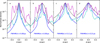Fig. 4 Normalised density profiles (blue lines) for cloud models A-D, for LOS towards filament (position indicated in Fig. 5). Examples of profiles at FWHM distance from the filament spine are plotted with dashed black lines. The density profiles for the other orthogonal directions, along constant right ascension (magenta lines) and constant declination (cyan), are for the model A with THEMIS dust. The quoted FWHM values correspond to the blue curve.

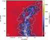Fig. 5 OMC-3 surface brightness at 350 μm (colour scale). The grey contours correspond to NIR extinction AJ=2.5 mag and 5 mag. The black crosses show the locations of potential embedded radiation sources that were included in some models. The magenta lines trace the filament spines that were used to generate the initial model density distributions. The white plus sign shows the position for the LOS density profiles in Fig. 4.

3.4 Dust models

Our goal was to find out to what extent the dust properties in OMC-3 can be constrained with the available observations and if some dust models are incompatible with the data. The RT modelling was therefore repeated for a number of dust models.

Some of the dust models have been tuned to reproduce observations of the Galactic diffuse medium, such as the Compiègne et al. model (Compiègne et al. 2011, COM below) and the THEMIS 2.0 model (see Table 3 in Ysard et al. 2024). Other models are more representative of dense regions in which the grains are thought to have evolved by coagulation and possibly by accretion of ice mantles. We use three types of model for these evolved cases.

The first type is described in Köhler et al. (2015) and is based on the optical properties of THEMIS 1.0 (Jones et al. 2013)³. It includes three types of large grains: CMM (core/mantle/mantle grains), where nano-grains are considered to have accreted onto the surface of the big carbons and silicates; their aggregated forms, AMM; and these same aggregates with an additional water ice mantle (AMMI). A summary of the properties of these grains is given in Sect. 2.3 of Jones et al. (2017).

The second type of model is described in Ysard et al. (2019) and is still based on THEMIS 1.0 (Jones et al. 2013). Three types of large grains are considered: (i) Mix 1, which is large spherical grains composed, by volume, of 2/3 silicate and 1/3 carbon; (ii) Mix 1:50, which is the same as the previous ones but with a porosity of 50%; (iii) Mix 1:Ice, which is the same compact grains as Mix 1, to which a mantle of water ice representing 55% of their volume has been added.

The third type of model is built on the same principle as Mix 1(:50:Ice) coarse grains but using the optical properties of THEMIS 2.0 (Ysard et al. 2024), not THEMIS 1.0. Four types of coarse grains are considered: (i) mixed-mantle grains (MC), in which the grains are a mixture of carbon and silicate; (ii) mixed-core porous (MCP), which are the same as MC but with a porosity of 25%; (iii) mixed-core ice (MCI), MC to which a mantle of water ice representing 50% of their volume has been added; (iv) MCPI, MC to which a mantle of water ice representing 50% of their volume has been added. Appendix B shows further examples of opacities and scattering functions (as traced by the asymmetry parameter g) for these dust models.

Figures 6 7 show examples of dust extinction curves and the 250−500 μm dust opacity spectral index β. The β values are mainly in the range of β ∼ 1.5 to β ∼ 2.2. Through their effect on dust temperatures, they also have an effect on the fitted ISRF levels.

One key dust parameter is the opacity ratio between the short wavelengths, where dust absorbs energy, and the long wavelengths, where the energy is again re-emitted away. In the present study, the NIR observations directly constrain the absolute level of extinction, while the quality of the FIR fits is mainly affected by the shape of the FIR extinction curve. Figures 6 7 use τ(250 μm)/τ(J) as a proxy for the FIR-to-NIR ratio. The ratio has been estimated to be τ(250 μm)/τ(J) ∼ 0.4 × 10⁻³ or slightly higher in diffuse clouds (e.g. Planck Collaboration XI 2014), but the ratio tends to be higher in molecular clouds. Juvela et al. (2015b) found a four times higher median ratio, τ(250 μm)/τ(J) ∼ 1.6 × 10⁻³, for a sample of dense clumps observed with Herschel. Most plotted dust models have τ(250 μm)/τ(J) ratios that are more consistent with observations of low-density clouds, but the ratio τ(250 μm)/τ(J) increases rapidly with increasing grain sizes. A complete list of the β and τ(250 μm)/τ(J) values of the dust models tested is included in Appendix C.

The dust properties were initially kept spatially constant, but later we also tested models with a smooth transition from one set of dust properties at low densities to another at higher densities. The transition was implemented by adjusting the relative abundances of two dust models; the relative abundances [0,1] of the first dust are $$\chi =\frac{1}{2}-\frac{1}{2}tanh[\xi \times ({log}_{10}{n}_{\mathrm{H}}-{log}_{10}{n}_0)].$$(5) The second dust has abundances 1−χ and thus becomes dominant at high volume densities. The density threshold of the transition is given by n₀ and the parameter ξ, which determines the steepness of the transition and was set to ξ=4.

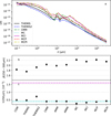Fig. 6 Extinction curves for selected dust models (frame a). Frame b shows the values of the FIR opacity spectral index. Frame c shows the FIR-NIR optical depth ratios τ(250 μm)/τ(J), where the cyan dashed line is drawn at τ(250 μm)/τ(J)=0.4 × 10−3 and the magenta dashed line at τ(250 μm)/τ(J)=1.6 × 10−3. The THEMIS2 models (MC to MCPI) have their default grain size distributions with a0 ∼ 0.05 μm.

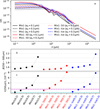Fig. 7 As Fig. 6 but for THEMIS dust models Mix 1, Mix 1:50, and Mix 1:Ice. Data are shown for size distributions with a0=0.1, 0.3, 0.5, 0.7, and 1.0 μm (numbers quoted within parentheses).

3.5 Model fits

Radiative transfer models were optimised to find the best match to the 250−500 μm FIR data. The free parameters in the fits are one scalar factor k_ISRF for the radiation field intensity and one scaling factor k_N for the column density associated with each map pixel.

The factor k_ISRF was optimised based on the ratios of the observed and model-predicted I_v(250 μm)/I_v(500 μm) ratios that were averaged over the Q=1−2 regions (Fig. 2). The optimisation thus concentrated on the dense parts of the field, also because the observations of low column density areas are more likely to be affected by large-scale density and radiation-field variations outside the modelled volume. The k_N values were updated based on the ratio of the observed and model-predicted 350 μm surface brightness, and therefore the models have a nominal resolution of 30^′′.

The combination of LOS cloud shapes, $A_{\mathrm{V}}^{\text{ext}}$ values, and dust models resulted in a large number of models (cf. Table C.1). The quality of each fit was quantified using the relative error $$r=100\%\times \frac{I_v^{\mathrm{MOD}}-I_v^{\mathrm{OBS}}}{I_v^{\mathrm{OBS}}},$$(6) where $I_v^{\mathrm{OBS}}$ and $I_v^{\mathrm{MOD}}$ are the observed and model-predicted surface brightness maps, respectively. The comparison was done at 30^′′ resolution, except at 500 μm where the model maps were convolved down to the 41^′′ resolution of the corresponding Herschel map. The quantity b=〈 r〉 is the bias and σ_r the standard deviation of the r values. These can be evaluated separately for a given wavelength and for different regions (different Q values; Sect. 2.2). We also used the mean squared error (MSE). While σ measures variation relative to the mean residual, MSE measures the variation relative to zero and is thus also affected by systematic errors (bias). The model optimisation was stopped when the 350 μm maps indicated good convergence with b(350 μm)<0.3% and σ(r(350 μm))<1%. The change in the radiation field intensity per iteration was also required to be small, with Δ k_ISRF<0.2%. One typically reached σ(r) ∼ 0.5%, except for a subset of models where the residuals in the densest filaments remained positive due to the saturation of the surface brightness (i.e. the model surface brightness remaining below the observed values).

The model predictions were also compared to the observations of the 160 μm surface brightness and the NIR extinction. These data, however, were not used in the optimisation itself.

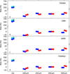Fig. 8 Bias $\langle (I_v^{\mathrm{MOD}}-I_v^{\mathrm{OBS}})/I_v^{\mathrm{OBS}}\rangle$ for four dust models (frames a-d). The symbols correspond to the cloud models A-D (circles, squares, triangles, and diamonds, respectively) that show here only minor differences. The x-axis label τ(J) refers to the filament (Q=1) J-band opacity, where the models are compared to the extinction derived with background stars and the Indebetouw et al. (2005) extinction curve, using either the NICER map (blue symbols) or median value of individual stars over the selected region (cyan symbols). For 160−500 μm the errors are shown for the filament (Q=1, blue symbols) and the ridge (Q=2, red symbols) regions, assuming an external extinction of $A_{\mathrm{V}}^{\text{ext}}=0.5^{\mathrm{m}}$ (open symbols) or $A_{\mathrm{V}}^{\text{ext}}=1.0^{\mathrm{m}}$ (filled symbols). The symbols are spread along the x-axis for better readability.

4 Results

4.1 Models with constant dust properties

We first examined models with spatially constant dust properties. Figure 8 shows the fit bias in the case of four dust models, using four cloud density fields (A−D; cf. Table 1), and for the values $A_{\mathrm{V}}^{\text{ext}}=0.5^{\mathrm{m}}$ and 1^m of the external attenuation. The results, and especially the τ(J) bias, are seen to depend mainly on the dust model, with smaller variations due to cloud shape and $A_{\mathrm{V}}^{\text{ext}}$ values. The models of Fig. 8 tend to slightly underestimate the 160 μm intensity, while the NIR opacity τ(J) is more significantly overestimated.

Figure 9 shows results for a set of 13 dust models. The figure also probes the effects of different grain size distributions (e.g. a₀=0.1 μm vs. a₀=0.3 μm), but regarding the NIR opacity, the results are still affected more by dust type than by size changes. The Mix 1 models of frames c and d are in good agreement with the τ(J) measurements and with only moderate positive bias for the extrapolated 160 μm surface brightness, mainly in the ridge region.

Figure 10 shows the fit quality, estimated radiation field intensity, and filament mass for selected models. The FIR residuals are plotted separately for the filament and ridge regions (Q=1 and Q=2, respectively). The model-predicted τ(J) values are compared with the average VISION extinction value over the Q=1 area, where the mean value over the Q=−1 area is subtracted as the background. Each line on the y-axis corresponds to one dust model, including all cloud models A-D and $A_{\mathrm{V}}^{\mathrm{ext}}=1^{\mathrm{m}}$. There is noticeable variation in fit quality. The MSE values range from ∼ 5% up to 10% and even 20% in the ridge region (Fig. 10a). The bias ranges from close to zero to ± 5% and even beyond (Fig. 10b). The σ values are typically 5−10% and tend to be higher at 250 μm than at 500 μm (Fig. 10c).

Frame d shows the ratio between the J-band optical depth in the Q = 1 area in the model and as estimated from the reddening of the background stars, using the NICER method and the extinction curve of the dust model in question. In most cases the NIR extinction is overestimated, and especially models with a₀ ≥ 0.5 μm appear to be clearly excluded.

If τ(250 μm)/τ(J)=1.6 × 10⁻³ were assumed to be the correct value also for OMC-3, then models with large grains, such as Mix 1, Mix 1:50, and Mix 1:Ice with a₀=0.3 μm would be preferred (Fig. 10e). However, in Juvela et al. (2015a) this ratio was derived assuming the normal NIR extinction curve and is therefore internally inconsistent in the case of large grain sizes. If large grains a₀ ≳ 0.3 μm were present everywhere in the OMC-3 field, the NIR extinction curve would be flat (cf. Fig. 7), and the NICER map should show only little correlation with the column density derived from dust emission. Based on Fig. 3, this loss of correlation may be observed in the ridge region. However, the ridge is probed by only a small number of background stars, and this prevents strong conclusions. Large grain sizes would also result in higher estimates for the filament mass and especially the radiation field intensity (Figs. 10f–g).

Figure 10 does not include models that failed the convergence criteria. Of the more than 500 models examined, only 23 showed greater than 5% positive 350 μm residuals in the ridge area. This indicates saturation of the model-predicted signal, the surface brightness no longer increasing with increasing column density. These cases corresponded mainly to the dust models MC, MCI, MCP, or MCPI with a₀=0.1 or 0.3 μm, often combined with a harder radiation field with $A_{\mathrm{V}}^{\text{ext}}=-0.5^{\mathrm{m}}$.

The approaching saturation of surface brightness can increase the mass ratio between the ridge and filament regions, even for some models included in Fig. 10. This is not likely to be due to internal heating. First, the masses were estimated for areas where the MIR and FIR point sources were already masked. Second, when we tested models with internal heating sources (Sect. 3.3) and optimised their luminosities based on their local impact on surface brightness, the effect on the total mass in the Q=1 and Q=2 regions remained always insignificant.

Figure B.3 in Appendix B shows selected data for 80 models with the lowest MSE values (combining the 250 μm and 500 μm errors in the Q=1−2 regions). These low-MSE models employ different versions of the Mix 1, Mix 1:Ice, and Mix 1:50 dust models with grain size distributions a₀=0.1−0.7 μm. In this sample, the MSE values vary only little, but the match to the observed A_J values is sensitive to the grain size. At 160 μm the models often overestimate the filament (Q=1) surface brightness by nearly 30%, while in the ridge region (Q=2) the residuals are scattered more around zero. Several of the a₀=0.1 μm dust models match the observed NIR extinction to within 30%. However, cases a₀ ≥ 0.3 μm tend to result in large positive or negative extinction estimates, which would exclude the presence of such large grains over the whole field.

There is no strong preference between different LOS density profiles. All A-D cloud models appear among the best-fitting models. The values of external extinction $A_{\mathrm{V}}^{\text{ext}}=0.5\mathrm{mag}$ and $A_{\mathrm{V}}^{\mathrm{ext}}=1\mathrm{mag}$ are also equally common. There are even a few models with $A_{\mathrm{V}}^{\mathrm{ext}}=-0.5\mathrm{mag}$, the case with the harder radiation field. The fit quality is relatively insensitive to the assumed spectral shape of the radiation field because the absolute level of the radiation field was always adjusted as a separate free parameter.

Fig. 9 As Fig. 8, but showing results for larger sample of dust models. The cloud model is A with $A_{\mathrm{V}}^{\mathrm{ext}}=1\mathrm{mag}$.

4.2 Models with spatial dust variations

Spatial dust property variations were examined using combinations of two dust models whose relative abundances were varied based on the volume density (Sect. 3.4). Because previous tests showed only little dependence on the other model parameters, the tests were done using only the cloud model $A_{\mathrm{V}}^{\mathrm{ext}}=1\mathrm{mag}$.

Figure 11 shows the results for the examined dust combinations. The density threshold n₀ for the transition between the two dust models was varied from 10³ to 3.2 × 10⁴ cm⁻³ in steps of a factor of two. Thus, for the highest (lowest) threshold, the results are similar to the single-dust models that used the same dust model as now in the low-density (high-density) region.

The combination of THEMIS dust at low densities and some Mix dust at high densities results in marginally the lowest bias values and the lowest dispersion σ in the residuals. However, the fits get consistently better with lower n₀, approaching the Fig. 10 results where the same Mix dust is used for the whole model. The lower n₀ requires in this case a higher radiation field intensity, up to k_ISRF ∼ 400. The same is observed for the combination of CMM and Mix 1:50 or Mix 1:Ice, where the best fits are obtained for low values of n₀ that again correspond to high values of k_ISRF.

The combinations of THEMIS2 at low densities and MC, MCI, MCP, or MCPI dust at high densities have relatively low σ values. They provide a good fit to the observed NIR extinction, but also show higher overall MSE values. Their τ(250 μm)/τ(J) ratios are slightly below the range of values that Juvela et al. (2015b) found for dense clumps (the shaded area in Fig. 11e). However, the OMC-3 field is also quite different from that previous sample, which consisted mainly of clumps in much less active environments. What is not visible in Fig. 11 is that for n₀ ≲ 8000 cm⁻³ the modelled surface brightness saturates for these dust combinations, resulting in significant positive residuals along the ridge. This was observed less in the case of single-dust models and is thus acerbated by stronger attenuation of the radiation field in the outer parts of the cloud (due to the THEMIS2 dust) and the resulting low temperature and weak emission of the MC dust along the ridge. In this case, the single-dust models perform better than their combination.

The tested dust combinations provide roughly equally good fits to the FIR data, and the main discriminator is the NIR extinction. However, the extinction can also be matched with almost pure Mix 1, Mix 1:50, or Mix 1:Ice dust, which also have τ(250 μm)/τ(J) ratios similar to those found in other dense clumps (Juvela et al. 2015b).

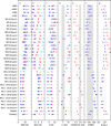Fig. 10 Results for single-dust cases for cloud models A−D and $A_{\mathrm{V}}^{\text{ext}}=1$ mag. Frames a-c show the bias, the standard deviation σ of the residuals, and the MSE values. These are shown for 250 μm (red and magenta dots for Q=1 and Q=2, respectively) and for 500 μm (blue and cyan dots for Q=1 and Q=2, respectively). Frame d shows the ratio of the J-band extinction predicted by the cloud model and the median estimate, based on background stars and the extinction curve of the dust model in question. The shading corresponds to a factor of two uncertainty, and the red arrows indicate values outside the plotted range. Frame e shows the mean ratio τ(250 μm)/τ(J) in the Q=1 area, relative to the reference value τ(250 μm)/τ(J)=1.6 × 10−3 (red points; with τ(J) for the standard extinction curve), the shading corresponding to 1−2.3 × 10−3 (Juvela et al. 2015b). Frame f shows the kISRF values for $A_{\mathrm{V}}^{\text{ext}}=$ 1 mag fits, the shading indicating the range 60− 260. The masses of the model clouds are shown in Frame g (blue for the Q=1 and red for the Q=2 area).

5 Discussion

We used RT modelling to investigate dust emission in the OMC-3 region. The starting points were the Herschel FIR observations of dust emission, but also the model predictions for the NIR extinction were later compared to the observations.

The FIR emission maps could be reproduced by almost all of the dust models tested, with only small variations in fit quality. The dust models mainly varied in how they matched the outer filament (Q=1) relative to the ridge (Q=2). The largest fit residuals were typically seen towards the high-density ridge, where the surface brightness is close to the maximum that some dust models can produce before saturation. Actual saturation was observed, especially when the THEMIS2 dust model in the outer cloud regions was combined with MC, MCI, MCP, or MCPI dust in the high-density part. An abrupt change in model dust properties could also result in unphysical filament profiles with a sharp jump in the density. In our models this was not clearly visible, partly due to the gradual change in the density-dependent relative abundances of the dust components and partly because the contributions from the material below and above n₀ change smoothly in the 2D projection.

One caveat is that our calculations do not include the thermal coupling between gas and dust, which could be important at high densities if the gas temperature without the coupling were much higher. Goldsmith (2001) estimated that at densities n(H₂) ∼ 10⁶ cm⁻³ the dust temperature could increase by more than one degree. The result corresponded to the normal ISRF attenuated by a factor of 10⁻⁴. In OMC-3 the radiation field could be two orders of magnitude stronger, but this is also compensated for by higher extinction. The visual extinction reaches A_V ∼ 10 mag at ∼ 1.5^′ distance from the filament centre (attenuation by a factor of ∼ e^10/2.5 ≈ 55). At that point, most UV photons have already been absorbed, thus eliminating most of the photoelectric heating. It therefore seems unlikely that the gas-to-dust coupling would cause noticeable effects within the central filament.

Several parts of the ridge (Q=2) were masked due to resolved MIR point sources or very strong FIR emission. These areas were excluded when the intensity of the external field was optimised. The additional heating from young stars and partly unresolved protostellar sources could be important in those areas and might explain the failure of some models to converge due to positive 350 μm residuals in the Q ≥ 2 areas (Table C.1). However, when embedded sources were included in models and the luminosities were optimised based on the local surface brightness, the effect of the sources remained very localised. The effect of strong sources had already been eliminated by direct masking (Q>2), and their impact on the wider filament region (Q=1) should be low.

Figure B.2 in Appendix B shows an example of the fit residuals. Embedded sources are not part of that model, and any local heating should result in compact positive residuals at short wavelengths. However, the errors show mainly extended structures that are probably correlated with variations in the cloud structure and external heating that are not perfectly matched by the model. The residual maps are smooth, especially at 500 μm, where the errors vary by no more than ∼ 10% across the filaments.

Because the column density updates were based on 350 μm data, the 250 μm and 500 μm residuals are anticorrelated. The 160 μm residuals tend to have a spatial distribution similar to the 250 μm residuals, but, due to the greater distance from the 350 μm reference wavelength, a larger magnitude. The shorter wavelengths are also more sensitive to variations in the radiation field and in the diffuse outer cloud layers that may be partly outside the modelled volume. In Fig. B.2, the 160 μm residuals are, on average, close to zero towards the centre of the map (where k_ISRF was determined) but increase strongly towards the map edges. Figure B.3 shows that for the best single-dust models the 160−250 μm bias tends to be higher (less negative or more positive) in the ridge (Q = 2) compared to the surrounding filament (Q = 1). The 160 μm bias values are around −30% in the filament. In the ridge, the 160 μm bias is close to zero for the best models, with an overall range from −5% to 30%. The 250 μm bias is small in the filament, between −1% and +2%, but systematically positive in the ridge, with values up to ∼ 5%. Errors at the level of a few per cent could be attributed to uncertainties in the calibration and, especially at 160 μm, to uncertainty in the background subtraction (Sect. 2.1.2), but the larger errors are significant. Models that give the correct 250 μm intensities in the filament region also tend to match the 160 μm observations of the ridge. In detail, these relative errors depend on the choice of grain materials and the shape of the size distribution.

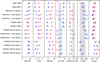Fig. 11 As Fig. 10, but for models with two dust components with density-dependent abundances. Results are shown for the cloud model C with $A_{\mathrm{V}}^{\mathrm{ext}}=1\mathrm{mag}$ and density thresholds n0= 103−3.2 × 104 cm−3, with symbols for higher n0 values shifted to slightly higher y-axis positions. In frame d, τ(J) is calculated using the actual dust models and the spatially varying extinction curves. The vertical lines in frames d-e indicate the corresponding single-dust results from Fig. 10 for the first (cyan lines) and the second (magenta lines) of the dust components.

5.1 Effects of cloud shape and radiation field spectrum

Modelling of low-mass star-forming clouds has shown clear dependence on the LOS density distribution of the clouds, as well as some dependence on the spectrum of the illuminating radiation field (Juvela et al. 2020; Juvela 2024). In contrast, in the OMC-3 models these were only marginal factors, as shown byFigs. 8–10. This is likely caused by the higher column density of the OMC-3 filaments, which results in almost all of the incoming radiation being already absorbed in outer cloud layers. Although the observed intensity does depend on the total column density, the FIR radiation observed towards the filaments originates in the first approximation in plane-parallel layers on the front and back cloud surfaces. Low-mass clouds are more transparent to dust-heating radiation, and a volume element is more likely to receive radiation from multiple directions, making the heating more dependent on the overall cloud shape.

Higher column density also decreases the dependence on the spectral shape of the illuminating radiation field. For example, the peak of a T_eff=38 000 K star is in UV and a T_eff=5000 K black body peaks at ∼ 1 μm. However, when the cloud has high column density, UV and optical radiation is absorbed in the cloud surface layers. The rest of the cloud is heated by the remaining NIR-MIR radiation, and there is no longer any difference between the extincted T_eff=38000 K and T_eff=5000 K black bodies. This applies to the shape of the radiation field, while the absolute level of the field is always a free parameter.

5.2 Constraints from the radiation field intensity

The models show a wide range of predictions for the radiation field intensity. This is partly due to the fitted 250−500 μm data covering only a narrow range of wavelengths. Since column densities are also free parameters, a small change in the dust model β can correspond to a large change in the fitted k_ISRF. The k_ISRF values also depend on the NIR-to-FIR opacity ratios. If this ratio is large, the external radiation field is strongly attenuated, and one can match the observed filament brightness only by increasing both its column density and the absolute level of the external field.

The parameter k_ISRF corresponds to the radiation field at the outer boundary of the models. We can make an independent estimate of the radiation field using background-subtracted surface brightness measurements. Figure A.1 shows selected NIR-mm spectral energy distributions (SEDs) for the OMC-3 field, making use also of Spitzer, WISE, and AKARI mid-infrared observations. If all the incoming radiation was absorbed and reradiated, the integral over the emission spectra should directly correspond to the k_ISRF values. The SED in the brightest southern part of the filament corresponds to a radiation field with k_ISRF=262. This is likely to be an upper limit, due to the presence of some local sources and the surface brightness generally increasing towards the south. A position selected from the filament wing gives k_ISRF=63 and the average over the PACS area k_ISRF=72. These are, in turn, likely to be lower limits if all of the incoming radiation is not absorbed at the lower column densities. As a rough estimate, the expected values are k_ISRF=100−200. In Fig. 10, some of the best dust models so far, Mix 1, Mix 1:50, and Mix 1:Ice, tend to require radiation fields above this range. On the other hand, most of the other dust models are closer to the lower limit, k_ISRF ∼ 100 or even below.

5.3 Evidence of NIR extinction

NIR extinction estimates were calculated based on the reddening of the light of background stars. The estimates depend on the assumed shape of the NIR extinction curve, and the variation between different dust models is illustrated in Appendix C. The extinction curves quoted in the literature correspond to only about 15% variations in extinction, and some of the tested dust models (e.g. THEMIS, THEMIS2, COM, CMM, and AMMI) give very similar values (Fig. C.1). However, the presence of larger grains a₀ ≳ 0.3 μm flattens the NIR extinction curve and can result in a wide range of values and even some negative extinction estimates. This affects the ratio of NIR opacities between the fitted model and the NICER estimates. For example, models that use Mix 1:Ice dust with a₀=0.3 μm have an NIR opacity below the NICER estimates. The increase in size to a₀=0.5 μm doubles the τ(250 μm)/τ(J) ratio, resulting in a significant reduction in column density and the model NIR opacity. However, the flattening of the extinction curve reduces the NICER estimates even more, so that the ratio between NIR model opacity and the NICER estimates increases above one, instead of decreasing further (e.g. Figs. 10 and B.3).

Figure 3 shows that at larger scales (corresponding to Q ≤ 1) the FIR filament is clearly visible in the Meingast et al. (2016) extinction map. This high degree of correlation therefore implies an upper limit of ∼ 0.1−0.3 μm for the mean grain size in the outer filament, the actual size limit depending on the dust model. In the ridge region (Q=2) the correlation disappears, which could be an indication that the grains have reached sizes ∼ 0.3 μm. However, the strength of this evidence is reduced by the low number of background stars detected in the Q ≥ 2 area (Fig. 2).

The size limits directly implied by the NIR data are roughly compatible with the evidence of the fitted cloud models. Figure 10 shows that in the Q=1 region the NIR opacity of the model clouds becomes inconsistent with the NIR stellar observations if the grain size is allowed to increase to a₀ ∼ 0.5 μm. For some dust models, such as MCI, MIX 1, Mix 1:50, and Mix 1:Ice, the preferred sizes are only slightly smaller, a₀ ∼ 0.1−0.3 μm.

The models with two dust components with spatially varying relative abundances attempted to better match the expectation of the largest grain growth being limited to the regions of highest volume density. In the models of Fig. 11, the dust properties at low volume densities are consistent with observations of the diffuse medium, and at high densities the grain size is increased to a₀=0.3 μm. The remaining free parameter was the density threshold n₀ of the transition. The evidence from the goodness of fit is not very clear, as lower bias may be associated with higher statistical errors, and the magnitudes of error in the Q=1 and Q=2 regions are often anticorrelated (Figs. 11a–c). However, with transition at low densities, n₀ ≤q 4000 cm⁻³, the models generally were in better agreement with the NIR extinction. The combination of two dust models naturally helps to retain the correlation between the NIR extinction and the cloud structure seen in FIR data, while still allowing larger grains and larger FIR emissivity in the central filament.

In principle, it would be useful to probe especially the Q=2 region using MIR point sources, to investigate the potential changes in the NIR-MIR extinction curve. However, the Spitzer maps of the ridge region contain only a handful of sources, mostly embedded young stellar objects rather than background stars. The MIR extinction of the extended background surface brightness provides additional constraints on dust properties but requires consideration of the additional contribution of dust scattering and thermal emission (Juvela & Mannfors 2023). We will address the extended MIR extinction in a future paper, in which the MIR emission from stochastically heated grains will also be modelled.

The NIR scattered light could also be used to constrain the combination of grain properties and the illuminating radiation field in the outer parts of the cloud, but accurate mapping of the extended NIR surface brightness needs dedicated observations. Our models covered only the dense part of the OMC-3 cloud, which is surrounded by column densities N(H₂) ∼ 10²¹ cm⁻² that also contribute to the NIR scattered surface brightness. Therefore, in the present paper NIR scattering has only a small indirect role by increasing the photometric noise and masking the faintest background stars.

6 Conclusions

We presented modelling of the NIR-FIR dust observations of the OMC-3 region, concentrating on its main filaments. The goal was to evaluate the possible range of dust properties and, as a secondary point, to put constraints on the cloud structure and the radiation field intensity. The study led to the following conclusions:

• The 160−500 μm observations of dust emission were always fitted satisfactorily, and this limited wavelength range alone is not sufficient to clearly reject any of the dust models;

• NIR extinction measurements are a valuable additional constraint. Most dust models correspond to NIR opacities that are clearly higher than the direct extinction measurements based on background stars;

• Large grain sizes result in the flattening of the NIR extinction curve. The good correlation between FIR emission and NIR extinction excludes the possibility of grain growth to mean sizes above a ∼ 0.1 μm in the outer part of the filament. For the central ridge, the correlation is almost non-existent and the presence of large grains is possible;

• The best overall fits to FIR observations were obtained with dust models Mix 1 and Mix 1:50 (large porous grains) with a mean grain size of a₀=0.3 μm and with the Mix 1:Ice model with slightly larger grains with a₀=0.5 μm. These have opacity ratios close to τ(250 μm)/τ(J) ∼ 1.6 × 10⁻³, the typical value previously seen in Herschel studies of dense clumps, when extinction is estimated using the standard extinction curve;

• Different dust models can result in very different predictions for the cloud mass and the local radiation field intensity. The RT runs with the otherwise best dust models, Mix 1, Mix 1:50, and Mix 1:Ice, require a slightly stronger radiation field in OMC-3 than the independently estimated 100−200 times the normal ISRF;

• The fit quality of models with spatially varying dust properties was not clearly better than in the best single-dust models;

• Overall, the combined FIR and NIR data are consistent with modest grain growth in the outer filament (a ≲ 0.3 μm) and do not exclude further increases in size in the central ridge.

In the present paper we concentrate on the properties of large dust grains that are in equilibrium with the radiation field and dominate the FIR emission. In a future study, we will expand the investigation to dust emission and scattering at MIR wavelengths to characterise the abundance and emission properties of small grains.

Acknowledgements

M.J. acknowledges the support of the Research Council of Finland Grant No. 348342.

References

Appendix A OMC-3 dust spectra

Figure A.1 shows examples of the SEDs using background-subtracted observations (Sect. 2.1.2), giving an idea of the general SED shape and its variations. Despite the high radiation field in the nearby Orion regions (both north and south of OMC-3), the dust emission peaks beyond 100 μm and thus corresponds to cool dust of ∼ 20 K for a wide range of dust models (cf. Schuller et al. 2021, their Fig. 2).

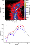Fig. A.1 Sample spectra in OMC-3 field. Frame a shows the Herschel 250 μm map and the outline of the PACS coverage. The white circles indicate the reference area used for background subtraction. Frame b shows spectra for background-subtracted data at the positions marked in frame a with blue, magenta, and red circles. The data correspond to 1’ (solid symbols; Spitzer, WISE, Herschel) or 2’ resolution (open symbols; AKARI, with 30% error bars). The average spectrum over the PACS coverage is drawn with a black dashed line.

Appendix B Additional plots on single-dust models

The optical properties of most dust models can be found through the DustEM⁴ and THEMIS ⁵ web sites and in the articles listed in Sect 3.4. The exceptions are MC, MCI, MCP, and MCPI that were calculated for this paper. Figure B.1 shows examples of optical properties for these four models, as well as for the THEMIS, THEMIS2, CMM, and AMMI models. In the plot, the scattering functions φ(θ) are characterised by the asymmetry parameters g=〈cos θ〉, where θ is the scattering angle. However, the model calculations used the effective scattering function, average φ weighted by the scattering cross-sections of grains of different sizes, rather than approximating the scattering function with a single Henyey-Greenstein function and the similarly weighted average g (e.g. Steinacker et al. 2013).

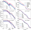Fig. B.1 Dust cross-sections κext, κabs, and κsca per hydrogen atom (left frames) and asymmetry parameters g=〈cos θ〉 (right frames) for selected dust models. The uppermost frames show the data for the THEMIS, THEMIS2, CMM, and AMMI models. The other frames show the corresponding data for the MC, MCI, MCP, and MCPI models, for the a0=0.1 μm (frames c-d) and a0=0.3 μm (frames e-f) size distributions.

As an example of fits with constant dust properties, Fig. B.2 shows the residuals, optical depths, and density cross-sections for a run using Mix 1 dust with a₀=0.3 μm. The results are shown for cloud model B and $A_{\mathrm{V}}^{\text{ext}}=1$ mag of external extinction.

Figure B.3 shows data for 80 models with spatially constant dust properties. The cases are selected based on their lowest MSE values, which are obtained by taking the average of the 250 μm and 500 μm MSE values in the Q=1 and Q=2 areas.

Appendix C Dust models and NIR extinction

Table C.1 lists key parameters for the dust models tested. These include the spectral index in the 250−500 μm wavelength interval and the ratio of the J-band and 250 μm dust opacities, τ(250 μm)/τ(J). The table gives a summary of the parameter combinations tested in the case of the single-dust models and indicates the cases showing saturation (i.e. imperfect fit to the observed 350 μm data). Only the case with $A_{\mathrm{V}}^{\mathrm{ext}}=1\mathrm{mag}$ was calculated for every combination of dust properties and A-D versions of cloud LOS density profiles.

In Fig. C.1 the shaded area shows extinction estimates for the set of extinction curves listed in Table 5 of Wang & Jiang (2014).

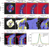Fig. B.2 Results for cloud model B with $A_{\mathrm{V}}^{\text{ext}}=$ 1 mag and a0=0.3 μm Mix 1 dust model. Frames a-d show the observed surface brightness maps and frames e-h the corresponding relative 160−500 μm residuals, $(I_v^{\text{OBS}}-I_v^{\text{MOD}})/I_v^{\text{OBS}}$. Frame i shows a map of the 250 μm optical depth from the direct MBB fitting of observations (41′′ resolution), and frame j shows the same for the fitted model (30′′ resolution). The last frame shows one-dimensional cross-sections of the model densities along the lines marked with white lines in the previous frames, along the LOS central plane of the model.

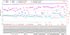Fig. B.3 Best single-dust models in order of increasing MSE, based on average of 250 μm and 500 μm residuals in Q=1−2 areas. Each model is labelled by the combination of the dust and cloud names and the $A_{\mathrm{V}}^{\text{ext}}$ value. The MSE markers and their colours indicate the model versions A-D. The 250 μm and 160 μm bias values are also plotted using the left y-axis, separately for the filament (Q=1) and the ridge (Q=2) regions. The 160 μm bias values are scaled by 0.1 for the plotting. The red crosses and the right y-axis show the bias in the predicted J-band extinction, b(τJ)=(A(J, model)−A(J, obs.))/A(J, obs.) over the Q=1 area. A(J, obs.) is estimated using the extinction curve of the dust model in question and all stars in the filament region (Q=1). Red arrows indicate values outside the plotted range.

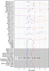Fig. C.1 Mean extinction A(J) in Q=0 (blue symbols) and Q=1 (red symbols) areas. Each row corresponds to a different extinction curve. The bottom shaded area includes the different observed extinction curves listed in Table 2 in Wang & Jiang (2014), and the upper rows are a selection of the dust models used in this paper. All extinction estimates are background-subtracted, and these can diverge, even with negative values, for models with grains sizes a0 ≳ 0.1 μm.

These refer mainly to observations at low column densities. However, one case has the ratio of total to selective extinction R_V=5.5, which should correspond to a dense environment with significant grain growth (Weingartner & Draine 2001). All these extinction curves result in less than 15% variation in the NIR extinction estimates. The Indebetouw et al. (2005) colour ratios used by Meingast et al. (2016) are among this group.

Figure C.1 includes additional extinction estimates for a set of dust models used in this paper. Models with mean grain sizes below ∼ 0.1 μm give values similar to those discussed above. However, larger grains result in rapid changes in the estimates. The values of the Q=1 region first increase and, for grain sizes a₀ ≳ 0.3 μm, can jump to even negative values. This agrees qualitatively with behaviour seen in Fig. 7a. As the NIR extinction curve becomes flat, there is no longer a clear correlation between the observed stellar colours and the extinction.

All Tables

All Figures

Fig. 1 Examples of OMC-3 observations. The maps show background-subtracted surface brightness values (non-linear colour scale) smoothed to the resolution used in the model fits. The plotted area is identical to previous figures. Frame c shows the outline of the PACS coverage and the reference areas for the SPIRE background subtraction (larger white circle) and for the adjustment of the PACS zero level (smaller white circle).

In the text

Fig. 2 Masks for the OMC-3 field. The levels correspond to areas with low emission (Q=−1), extended cloud (Q=0), filament (Q=1), ridge (Q=2), bright parts of the ridge (Q=3), FIR point sources and highsurface brightness areas affected by local heating (Q=4), and MIR point sources (Q=5). The small dots correspond to the NIR star-like (cyan) and potentially extended (blue) sources that are the basis of the NIR extinction map (Meingast et al. 2016).

In the text

Fig. 3 Comparison of τ(250 μm) optical depth map derived from Herschel observations at 41′′ resolution (frame a) and NICER extinction map of Meingast et al. (2016) at 1’ resolution (frame b). The white and grey contours show, respectively, the outlines of the filament (Q=1) and the ridge (Q=2) regions. The black contours separate other high column density areas that are excluded from the analysis (Q>2).

In the text

Fig. 4 Normalised density profiles (blue lines) for cloud models A-D, for LOS towards filament (position indicated in Fig. 5). Examples of profiles at FWHM distance from the filament spine are plotted with dashed black lines. The density profiles for the other orthogonal directions, along constant right ascension (magenta lines) and constant declination (cyan), are for the model A with THEMIS dust. The quoted FWHM values correspond to the blue curve.

In the text

Fig. 5 OMC-3 surface brightness at 350 μm (colour scale). The grey contours correspond to NIR extinction AJ=2.5 mag and 5 mag. The black crosses show the locations of potential embedded radiation sources that were included in some models. The magenta lines trace the filament spines that were used to generate the initial model density distributions. The white plus sign shows the position for the LOS density profiles in Fig. 4.

In the text

Fig. 6 Extinction curves for selected dust models (frame a). Frame b shows the values of the FIR opacity spectral index. Frame c shows the FIR-NIR optical depth ratios τ(250 μm)/τ(J), where the cyan dashed line is drawn at τ(250 μm)/τ(J)=0.4 × 10−3 and the magenta dashed line at τ(250 μm)/τ(J)=1.6 × 10−3. The THEMIS2 models (MC to MCPI) have their default grain size distributions with a0 ∼ 0.05 μm.

In the text

	Fig. 7 As Fig. 6 but for THEMIS dust models Mix 1, Mix 1:50, and Mix 1:Ice. Data are shown for size distributions with a0=0.1, 0.3, 0.5, 0.7, and 1.0 μm (numbers quoted within parentheses).
In the text

Fig. 8 Bias $\langle (I_v^{\mathrm{MOD}}-I_v^{\mathrm{OBS}})/I_v^{\mathrm{OBS}}\rangle$ for four dust models (frames a-d). The symbols correspond to the cloud models A-D (circles, squares, triangles, and diamonds, respectively) that show here only minor differences. The x-axis label τ(J) refers to the filament (Q=1) J-band opacity, where the models are compared to the extinction derived with background stars and the Indebetouw et al. (2005) extinction curve, using either the NICER map (blue symbols) or median value of individual stars over the selected region (cyan symbols). For 160−500 μm the errors are shown for the filament (Q=1, blue symbols) and the ridge (Q=2, red symbols) regions, assuming an external extinction of $A_{\mathrm{V}}^{\text{ext}}=0.5^{\mathrm{m}}$ (open symbols) or $A_{\mathrm{V}}^{\text{ext}}=1.0^{\mathrm{m}}$ (filled symbols). The symbols are spread along the x-axis for better readability.

In the text

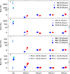	Fig. 9 As Fig. 8, but showing results for larger sample of dust models. The cloud model is A with $A_{\mathrm{V}}^{\mathrm{ext}}=1\mathrm{mag}$.
In the text

Fig. 10 Results for single-dust cases for cloud models A−D and $A_{\mathrm{V}}^{\text{ext}}=1$ mag. Frames a-c show the bias, the standard deviation σ of the residuals, and the MSE values. These are shown for 250 μm (red and magenta dots for Q=1 and Q=2, respectively) and for 500 μm (blue and cyan dots for Q=1 and Q=2, respectively). Frame d shows the ratio of the J-band extinction predicted by the cloud model and the median estimate, based on background stars and the extinction curve of the dust model in question. The shading corresponds to a factor of two uncertainty, and the red arrows indicate values outside the plotted range. Frame e shows the mean ratio τ(250 μm)/τ(J) in the Q=1 area, relative to the reference value τ(250 μm)/τ(J)=1.6 × 10−3 (red points; with τ(J) for the standard extinction curve), the shading corresponding to 1−2.3 × 10−3 (Juvela et al. 2015b). Frame f shows the kISRF values for $A_{\mathrm{V}}^{\text{ext}}=$ 1 mag fits, the shading indicating the range 60− 260. The masses of the model clouds are shown in Frame g (blue for the Q=1 and red for the Q=2 area).

In the text

Fig. 11 As Fig. 10, but for models with two dust components with density-dependent abundances. Results are shown for the cloud model C with $A_{\mathrm{V}}^{\mathrm{ext}}=1\mathrm{mag}$ and density thresholds n0= 103−3.2 × 104 cm−3, with symbols for higher n0 values shifted to slightly higher y-axis positions. In frame d, τ(J) is calculated using the actual dust models and the spatially varying extinction curves. The vertical lines in frames d-e indicate the corresponding single-dust results from Fig. 10 for the first (cyan lines) and the second (magenta lines) of the dust components.

In the text

Fig. A.1 Sample spectra in OMC-3 field. Frame a shows the Herschel 250 μm map and the outline of the PACS coverage. The white circles indicate the reference area used for background subtraction. Frame b shows spectra for background-subtracted data at the positions marked in frame a with blue, magenta, and red circles. The data correspond to 1’ (solid symbols; Spitzer, WISE, Herschel) or 2’ resolution (open symbols; AKARI, with 30% error bars). The average spectrum over the PACS coverage is drawn with a black dashed line.

In the text

Fig. B.1 Dust cross-sections κext, κabs, and κsca per hydrogen atom (left frames) and asymmetry parameters g=〈cos θ〉 (right frames) for selected dust models. The uppermost frames show the data for the THEMIS, THEMIS2, CMM, and AMMI models. The other frames show the corresponding data for the MC, MCI, MCP, and MCPI models, for the a0=0.1 μm (frames c-d) and a0=0.3 μm (frames e-f) size distributions.

In the text

Fig. B.2 Results for cloud model B with $A_{\mathrm{V}}^{\text{ext}}=$ 1 mag and a0=0.3 μm Mix 1 dust model. Frames a-d show the observed surface brightness maps and frames e-h the corresponding relative 160−500 μm residuals, $(I_v^{\text{OBS}}-I_v^{\text{MOD}})/I_v^{\text{OBS}}$. Frame i shows a map of the 250 μm optical depth from the direct MBB fitting of observations (41′′ resolution), and frame j shows the same for the fitted model (30′′ resolution). The last frame shows one-dimensional cross-sections of the model densities along the lines marked with white lines in the previous frames, along the LOS central plane of the model.

In the text

Fig. B.3 Best single-dust models in order of increasing MSE, based on average of 250 μm and 500 μm residuals in Q=1−2 areas. Each model is labelled by the combination of the dust and cloud names and the $A_{\mathrm{V}}^{\text{ext}}$ value. The MSE markers and their colours indicate the model versions A-D. The 250 μm and 160 μm bias values are also plotted using the left y-axis, separately for the filament (Q=1) and the ridge (Q=2) regions. The 160 μm bias values are scaled by 0.1 for the plotting. The red crosses and the right y-axis show the bias in the predicted J-band extinction, b(τJ)=(A(J, model)−A(J, obs.))/A(J, obs.) over the Q=1 area. A(J, obs.) is estimated using the extinction curve of the dust model in question and all stars in the filament region (Q=1). Red arrows indicate values outside the plotted range.

In the text

Fig. C.1 Mean extinction A(J) in Q=0 (blue symbols) and Q=1 (red symbols) areas. Each row corresponds to a different extinction curve. The bottom shaded area includes the different observed extinction curves listed in Table 2 in Wang & Jiang (2014), and the upper rows are a selection of the dust models used in this paper. All extinction estimates are background-subtracted, and these can diverge, even with negative values, for models with grains sizes a0 ≳ 0.1 μm.

In the text

References

- Andersen, M., Thi, W. F., Steinacker, J., & Tothill, N., 2014, A&A, 568, L3 [NASA ADS] [CrossRef] [EDP Sciences] [Google Scholar]
- André, P., Men’shchikov, A., Bontemps, S., et al. 2010, A&A, 518, L102 [NASA ADS] [CrossRef] [EDP Sciences] [Google Scholar]
- Aniano, G., Draine, B. T., Gordon, K. D., & Sandstrom, K., 2011, PASP, 123, 1218 [Google Scholar]
- Arzoumanian, D., André, P., Didelon, P., et al. 2011, A&A, 529, L6 [NASA ADS] [CrossRef] [EDP Sciences] [Google Scholar]
- Bernard, J. P., Abergel, A., Ristorcelli, I., et al. 1999, A&A, 347, 640 [NASA ADS] [Google Scholar]
- Bianchi, S., Gonçalves, J., Albrecht, M., et al. 2003, A&A, 399, L43 [NASA ADS] [CrossRef] [EDP Sciences] [Google Scholar]
- Bracco, A., Palmeirim, P., André, P., et al. 2017, A&A, 604, A52 [NASA ADS] [CrossRef] [EDP Sciences] [Google Scholar]
- Butler, M. J., & Tan, J. C., 2012, ApJ, 754, 5 [Google Scholar]
- Cambrésy, L., Boulanger, F., Lagache, G., & Stepnik, B., 2001, A&A, 375, 999 [NASA ADS] [CrossRef] [EDP Sciences] [Google Scholar]
- Compiègne, M., Verstraete, L., Jones, A., et al. 2011, A&A, 525, A103 [Google Scholar]
- Demyk, K., Meny, C., Lu, X.-H., et al. 2017, A&A, 600, A123 [NASA ADS] [CrossRef] [EDP Sciences] [Google Scholar]
- Demyk, K., Gromov, V., Meny, C., et al. 2022, A&A, 666, A192 [NASA ADS] [CrossRef] [EDP Sciences] [Google Scholar]
- Désert, F., Macías-Pérez, J. F., Mayet, F., et al. 2008, A&A, 481, 411 [NASA ADS] [CrossRef] [EDP Sciences] [Google Scholar]
- Dupac, X., Bernard, J., Boudet, N., et al. 2003, A&A, 404, L11 [NASA ADS] [CrossRef] [EDP Sciences] [Google Scholar]
- Flagey, N., Noriega-Crespo, A., Boulanger, F., et al. 2009, ApJ, 701, 1450 [Google Scholar]
- Goldsmith, P. F., 2001, ApJ, 557, 736 [Google Scholar]
- Großschedl, J. E., Alves, J., Meingast, S., et al. 2018, A&A, 619, A106 [Google Scholar]
- Hacar, A., Tafalla, M., Forbrich, J., et al. 2018, A&A, 610, A77 [NASA ADS] [CrossRef] [EDP Sciences] [Google Scholar]
- Indebetouw, R., Mathis, J. S., Babler, B. L., et al. 2005, ApJ, 619, 931 [NASA ADS] [CrossRef] [Google Scholar]
- Jones, A. P., Fanciullo, L., Köhler, M., et al. 2013, A&A, 558, A62 [NASA ADS] [CrossRef] [EDP Sciences] [Google Scholar]
- Jones, A. P., Köhler, M., Ysard, N., Bocchio, M., & Verstraete, L., 2017, A&A, 602, A46 [NASA ADS] [CrossRef] [EDP Sciences] [Google Scholar]
- Juvela, M., 2024, A&A, 681, A74 [NASA ADS] [CrossRef] [EDP Sciences] [Google Scholar]
- Juvela, M., & Mannfors, E., 2023, A&A, 671, A111 [NASA ADS] [CrossRef] [EDP Sciences] [Google Scholar]
- Juvela, M., Pelkonen, V. M., White, G. J., et al. 2012, A&A, 544, A14 [NASA ADS] [CrossRef] [EDP Sciences] [Google Scholar]
- Juvela, M., Demyk, K., Doi, Y., et al. 2015a, A&A, 584, A94 [NASA ADS] [CrossRef] [EDP Sciences] [Google Scholar]
- Juvela, M., Ristorcelli, I., Marshall, D. J., et al. 2015b, A&A, 584, A93 [NASA ADS] [CrossRef] [EDP Sciences] [Google Scholar]
- Juvela, M., He, J., Pattle, K., et al. 2018, A&A, 612, A71 [NASA ADS] [CrossRef] [EDP Sciences] [Google Scholar]
- Juvela, M., Neha, S., Mannfors, E., et al. 2020, A&A, 643, A132 [EDP Sciences] [Google Scholar]
- Kainulainen, J., & Tan, J. C., 2013, A&A, 549, A53 [NASA ADS] [CrossRef] [EDP Sciences] [Google Scholar]
- Kainulainen, J., Stutz, A. M., Stanke, T., et al. 2017, A&A, 600, A141 [NASA ADS] [CrossRef] [EDP Sciences] [Google Scholar]
- Köhler, M., Ysard, N., & Jones, A. P., 2015, A&A, 579, A15 [NASA ADS] [CrossRef] [EDP Sciences] [Google Scholar]
- Lagache, G., Abergel, A., Boulanger, F., & Puget, J., 1998, A&A, 333, 709 [NASA ADS] [Google Scholar]
- Lefèvre, C., Pagani, L., Min, M., Poteet, C., & Whittet, D., 2016, A&A, 585, L4 [NASA ADS] [CrossRef] [EDP Sciences] [Google Scholar]
- Lombardi, M., 2009, A&A, 493, 735 [NASA ADS] [CrossRef] [EDP Sciences] [Google Scholar]
- Lombardi, M., & Alves, J., 2001, A&A, 377, 1023 [NASA ADS] [CrossRef] [EDP Sciences] [Google Scholar]
- Mannfors, E., Juvela, M., Liu, T., & Pelkonen, V.-M., 2025, A&A, 695, A242 [NASA ADS] [CrossRef] [EDP Sciences] [Google Scholar]
- Martin, P. G., Roy, A., Bontemps, S., et al. 2012, ApJ, 751, 28 [NASA ADS] [CrossRef] [Google Scholar]
- Mathis, J. S., Mezger, P. G., & Panagia, N., 1983, A&A, 128, 212 [NASA ADS] [Google Scholar]
- Meingast, S., Alves, J., Mardones, D., et al. 2016, A&A, 587, A153 [NASA ADS] [CrossRef] [EDP Sciences] [Google Scholar]
- Murakami, H., Baba, H., Barthel, P., et al. 2007, PASJ, 59, 369 [Google Scholar]
- Pagani, L., Steinacker, J., Bacmann, A., Stutz, A., & Henning, T., 2010, Science, 329, 1622 [Google Scholar]
- Paradis, D., Bernard, J.-P., & Mény, C., 2009, A&A, 506, 745 [NASA ADS] [CrossRef] [EDP Sciences] [Google Scholar]
- Paradis, D., Veneziani, M., Noriega-Crespo, A., et al. 2010, A&A, 520, L8 [NASA ADS] [CrossRef] [EDP Sciences] [Google Scholar]
- Paradis, D., Paladini, R., Noriega-Crespo, A., et al. 2012, A&A, 537, A113 [NASA ADS] [CrossRef] [EDP Sciences] [Google Scholar]
- Pilbratt, G. L., Riedinger, J. R., Passvogel, T., et al. 2010, A&A, 518, L1 [NASA ADS] [CrossRef] [EDP Sciences] [Google Scholar]
- Planck Collaboration XVII., 2011, A&A, 536, A17 [NASA ADS] [CrossRef] [EDP Sciences] [Google Scholar]
- Planck Collaboration XIX., 2011, A&A, 536, A19 [NASA ADS] [CrossRef] [EDP Sciences] [Google Scholar]
- Planck Collaboration XI., 2014, A&A, 571, A11 [NASA ADS] [CrossRef] [EDP Sciences] [Google Scholar]
- Planck Collaboration Int. XXII., 2015, A&A, 576, A107 [NASA ADS] [CrossRef] [EDP Sciences] [Google Scholar]
- Planck Collaboration Int. XXIX., 2016, A&A, 586, A132 [NASA ADS] [CrossRef] [EDP Sciences] [Google Scholar]
- Reach, W. T., Dwek, E., Fixsen, D. J., et al. 1995, ApJ, 451, 188 [NASA ADS] [CrossRef] [Google Scholar]
- Roy, A., Martin, P. G., Polychroni, D., et al. 2013, ApJ, 763, 55 [Google Scholar]
- Saajasto, M., Juvela, M., Lefèvre, C., Pagani, L., & Ysard, N., 2021, A&A, 647, A109 [NASA ADS] [CrossRef] [EDP Sciences] [Google Scholar]
- Sadavoy, S. I., Di Francesco, J., Johnstone, D., et al. 2013, ApJ, 767, 126 [Google Scholar]
- Schuller, F., André, P., Shimajiri, Y., et al. 2021, A&A, 651, A36 [NASA ADS] [CrossRef] [EDP Sciences] [Google Scholar]
- Scibelli, S., Shirley, Y., Schmiedeke, A., et al. 2023, MNRAS, 521, 4579 [NASA ADS] [CrossRef] [Google Scholar]
- Scott, A., & Duley, W. W., 1996, ApJS, 105, 401 [NASA ADS] [CrossRef] [Google Scholar]
- Simon, R., Jackson, J. M., Rathborne, J. M., & Chambers, E. T., 2006, ApJ, 639, 227 [CrossRef] [Google Scholar]
- Steinacker, J., Andersen, M., Thi, W. F., et al. 2015, A&A, 582, A70 [NASA ADS] [CrossRef] [EDP Sciences] [Google Scholar]
- Steinacker, J., Pagani, L., Bacmann, A., & Guieu, S., 2010, A&A, 511, A9 [NASA ADS] [CrossRef] [EDP Sciences] [Google Scholar]
- Steinacker, J., Baes, M., & Gordon, K. D., 2013, ARA&A, 51, 63 [CrossRef] [Google Scholar]
- Stepnik, B., Abergel, A., Bernard, J., et al. 2003, A&A, 398, 551 [CrossRef] [EDP Sciences] [Google Scholar]
- Tauber, J. A., Mandolesi, N., Puget, J., et al. 2010, A&A, 520, A1 [NASA ADS] [CrossRef] [EDP Sciences] [Google Scholar]
- Wang, S., & Jiang, B. W., 2014, ApJ, 788, L12 [NASA ADS] [CrossRef] [Google Scholar]
- Weingartner, J. C., & Draine, B. T., 2001, ApJ, 548, 296 [Google Scholar]
- Werner, M. W., Roellig, T. L., Low, F. J., et al. 2004, ApJS, 154, 1 [NASA ADS] [CrossRef] [Google Scholar]
- Wright, E. L., Eisenhardt, P. R. M., Mainzer, A. K., et al. 2010, AJ, 140, 1868 [Google Scholar]
- Ysard, N., Abergel, A., Ristorcelli, I., et al. 2013, A&A, 559, A133 [NASA ADS] [CrossRef] [EDP Sciences] [Google Scholar]
- Ysard, N., Jones, A. P., Guillet, V., et al. 2024, A&A, 684, A34 [NASA ADS] [CrossRef] [EDP Sciences] [Google Scholar]
- Ysard, N., Koehler, M., Jimenez-Serra, I., Jones, A. P., & Verstraete, L., 2019, A&A, 631, A88 [NASA ADS] [CrossRef] [EDP Sciences] [Google Scholar]
The main difference between THEMIS 1.0 (Jones et al. 2013) and THEMIS 2.0 (Ysard et al. 2024) is the choice of optical properties for silicates. The first version of the model uses the properties described in Scott & Duley (1996) down to the mid-IR and an extrapolation of those into the FIR. The second version of the model uses the optical properties of silicates measured in the laboratory by Demyk et al. (2017, 2022) down to λ ∼ 1 mm.