| Issue |
A&A
Volume 706, February 2026
|
|
|---|---|---|
| Article Number | A381 | |
| Number of page(s) | 24 | |
| Section | Stellar structure and evolution | |
| DOI | https://doi.org/10.1051/0004-6361/202556425 | |
| Published online | 23 February 2026 | |
Normal or transitional? The evolution and properties of two type Ia supernovae in the Virgo cluster
1
DARK, Niels Bohr Institute, University of Copenhagen Jagtvej 155A 2200 Copenhagen, Denmark
2
INAF, Osservatorio Astronomico di Capodimonte Salita Moiariello 16 I-80121 Naples, Italy
3
School of Mathematics and Physics, University of Queensland Brisbane QLD 4072, Australia
4
Department of Astronomy, University of Illinois at Urbana-Champaign 1002 W. Green St. Champaign-Urbana IL 61801, USA
5
Institute for Astronomy, University of Hawaii 2680 Woodlawn Drive Honolulu HI 96822, USA
6
Kavli Institute for Theoretical Physics, University of California, Santa Barbara 552 University Road Goleta CA 93106-4030, USA
7
Las Cumbres Observatory, 6740 Cortona Drive Suite 102 Goleta CA 93117, USA
8
David A. Dunlap Department of Astronomy and Astrophysics, University of Toronto 50 St. George Street Toronto ON M5S 3H4, Canada
9
Institute of Astronomy and Kavli Institute for Cosmology Madingley Road Cambridge CB3 0HA, UK
10
Physics and Astronomy Department, Johns Hopkins University Baltimore MD 21218, USA
11
Space Telescope Science Institute Baltimore MD 21218, USA
12
Astrophysics Research Center of the Open University (ARCO), The Open University of Israel Ra’anana 4353701, Israel
13
Department of Natural Sciences, The Open University of Israel Ra’anana 4353701, Israel
14
Department of Astronomy and Astrophysics, University of California Santa Cruz CA 95064, USA
15
School of Physics, The University of Melbourne Melbourne VIC 3010, Australia
16
Graduate Institute of Astronomy, National Central University 300 Zhongda Road Zhongli Taoyuan 32001, Taiwan
17
INAF – Osservatorio Astronomico di Padova Vicolo dell’Osservatorio 5 I-35122 Padova, Italy
18
Gran Sasso Science Institute (GSSI) I-67100 L’Aquila, Italy
19
Osservatorio Astronomico S. di Giacomo, AstroCampania Via S. di Giacomo I-80051 Agerola, Italy
20
School of Physics and Astronomy, Birmingham University Birmingham B15 2TT, UK
21
Department of Physics, Lancaster University Lancaster LA1, UK
22
Department of Physics, University of Oxford Keble Road Oxford OX1 3RH, UK
23
Center for Interdisciplinary Exploration and Research in Astrophysics (CIERA) and Department of Physics and Astronomy, Northwestern University Evanston IL 60208, USA
24
Department of Astronomy, University of California Berkeley CA 94720-3411, USA
25
Dipartimento di Fisica e Astronomia, Universitá degli Studi di Padova Via F. Marzolo 8 I-35131 Padova, Italy
26
INAF – Osservatorio Astronomico di Brera Via E. Bianchi 46 I-23807 Merate (LC), Italy
27
Astrophysics Research Centre, School of Mathematics and Physics, Queen’s University Belfast Belfast BT7 1NN, UK
28
The Thacher School 5025 Thacher Rd. Ojai CA 93023, USA
29
Adler Planetarium 1300 South DuSable Lake Shore Drive Chicago IL 60605, USA
★ Corresponding author: This email address is being protected from spambots. You need JavaScript enabled to view it.
, This email address is being protected from spambots. You need JavaScript enabled to view it.
Received:
15
July
2025
Accepted:
28
November
2025
Abstract
Type Ia supernovae (SNe Ia) are among the most precise cosmological distance indicators used to study the expansion history of the Universe. The vast increase in SN Ia data due to large-scale astrophysical surveys has led to the discovery of a wide variety of SN Ia sub-classes, such as transitional and fast-declining SNe Ia. However, their distinct photometric and spectroscopic properties differentiate them from the population of normal SNe Ia such that their use as cosmological tools remains challenged. Here, we present a high-cadenced photometric and spectroscopic dataset of two SNe Ia, SNe 2020ue and 2020nlb, which were discovered in the nearby Virgo cluster of galaxies. Our study shows that SN 2020nlb is a normal SN Ia whose unusually red colour is intrinsic, arising from a lower photospheric temperature rather than interstellar reddening, providing clear evidence that colour diversity among normal SNe Ia can have a physical origin. In contrast, SN 2020ue has photometric properties, such as colour evolution and light curve decay rate, similar to those of transitional SNe. It is hence more spectroscopically aligned with normal SNe Ia. This is evident from spectroscopic indicators such as the pseudo-equivalent width of Si II lines. Thus, such SNe Ia, which lie photometrically at the edge of the standard normal SNe Ia range, may be missed in cosmological SNe Ia samples. Our results highlight that a spectroscopic analysis of SNe Ia around peak brightness is crucial for identifying intrinsic colour variations and constructing a more complete and physically homogeneous SN Ia sample for precision cosmology.
Key words: supernovae: general / supernovae: individual: SN2020ue / supernovae: individual: SN2020nlb / distance scale
© The Authors 2026
 Open Access article, published by EDP Sciences, under the terms of the Creative Commons Attribution License (https://creativecommons.org/licenses/by/4.0), which permits unrestricted use, distribution, and reproduction in any medium, provided the original work is properly cited.
This article is published in open access under the Subscribe to Open model. This email address is being protected from spambots. You need JavaScript enabled to view it. to support open access publication.
1. Introduction
Type Ia supernovae (SNe Ia) result from the thermonuclear detonation of carbon-oxygen (CO) white dwarfs (WDs), completely disrupting them (Nugent et al. 2011; Bloom et al. 2012; Maguire 2017; Branch & Wheeler 2017). Early spectra are characterised by the absence of hydrogen and helium, with prominent silicon and other iron-group and intermediate-mass elements (IME) (Filippenko 1997). The strength of these spectral signatures is likely connected to the progenitor system and explosion mechanism, both of which remain uncertain. Various progenitor scenarios and explosion mechanisms have been proposed due to the complex physics of SN Ia explosions (Livio & Mazzali 2018; Liu et al. 2023; Ruiter & Seitenzahl 2025). Leading scenarios include the single-degenerate (SD) (Whelan & Iben 1973) and double-degenerate (DD) systems (Iben & Tutukov 1984).
The SD scenario involves a Chandrasekhar-limit WD accreting matter from a non-degenerate companion star (a red giant or low-mass main-sequence star) until it reaches critical mass and undergoes carbon detonation. Conversely, the DD scenario is initiated by the dynamical merging of two WDs, triggering a thermonuclear runaway due to rapid temperature increase or accretion-induced collapse (see e.g. Ruiter & Seitenzahl 2025, and references therein). The classical model explaining CO WD explosions involves the delayed-detonation mechanism (Khokhlov 1991; Yamaoka et al. 1992; Iwamoto et al. 1999). This process begins with a subsonic deflagration, transitioning into supersonic detonation as the burning rate rapidly increases. The detonation wave propagates through the entire WD, enabling the burning of exterior material. This mechanism effectively explains the distribution of elements determined via high-cadence spectroscopic analysis and spectral synthesis modelling techniques (Stehle et al. 2005; Mazzali et al. 2008; Tanaka et al. 2011; Mazzali et al. 2015). This includes the confinement of Fe-peak elements, particularly the 56Ni radioactive isotope, within the innermost layers.
The progenitor system(s) and explosion mechanism(s) of SNe Ia influence the photometric evolution, including light curves. The synthesis of 56Ni, which decays into 56Co (Colgate & McKee 1969), and the diffusion of radiation within the SN ejecta (Branch & Wheeler 2017) drive the increase in brightness for 15−20 days (Woosley et al. 2007; Firth et al. 2015; Hillebrandt et al. 2013; Perets et al. 2019). As a result, the amount of synthesised 56Ni correlates with the peak brightness of SN Ia (Arnett 1982) and regulates the heating budget. High-energy photon diffusion from the ejecta’s core to its envelope results in thermalisation and optical detection as the ejecta becomes optically thin. Moreover, temperature affects opacities in the SN ejecta, influencing diffusion timescales (Höflich et al. 2013), which dictate the light curve decline rate. This provides a theoretical basis for the empirical SN Ia luminosity-decay relation (Pskovskii 1977; Phillips 1993). Brighter SN Ia peak magnitudes exhibit longer rise and decay times due to greater 56Ni synthesis, while fainter SNe Ia with faster rising and decaying light curves have produced smaller amounts.
‘Normal’ SNe Ia display a secondary NIR maximum 20−40 days post-optical peak brightness (Hamuy et al. 1993; Kasen 2006; Jack et al. 2012; Phillips 2012; Dhawan et al. 2015), which was first noted for SN1980N and SN1981B (Elias et al. 1985). This is likely due to significant iron-group element synthesis during the explosion, absorbing and re-emitting UV radiation in the near-infrared (NIR) via fluorescence (Kasen 2006). Subsequently, optical and NIR light curves enter a shallow, steady decay powered by the 56Co to 56Fe decay chain, characterised by a longer half-life (77.12 days) than the 56Ni to 56Co chain (6.10 days, Nadyozhin 1994). Around 15−17% of SNe Ia are sub-luminous, fast-declining events (Li et al. 2011a; Desai et al. 2024; Ma et al. 2025), with a gradual rather than sharp division between sub-luminous and normal SNe Ia (Graur 2024). Classical examples include SN 1991bg-like events (Filippenko et al. 1992a; Leibundgut et al. 1993), characterised by faint peak luminosities, rapid B-band decline rates (Δm15 > 1.5 mag), and redder colours (B − V ∼ 0.4 mag) than normal SNe Ia (Hoeflich et al. 2017). Lacking secondary NIR maxima, these events also exhibit prominent Ti II features in early spectra, indicating low photospheric temperatures (Leibundgut et al. 1993; Nugent et al. 1995). Intriguingly, such SNe Ia are predominantly found in early-type galaxies.
‘Transitional’ SNe Ia constitute another sub-class with mixed photometric and spectroscopic characteristics (Taubenberger et al. 2008; González-Gaitán et al. 2011; Hsiao et al. 2015; Ashall et al. 2016; Gall et al. 2018). They exhibit fast light curve decline rates (Δm15 ≳ 1.5 mag), brighter peak magnitudes than SN 1991bg-like events, and a secondary NIR maximum. Spectroscopically, they lack Ti II at similar epochs to SN 1991bg-like events but display enhanced higher ionisation features such as Fe III, as well as an intense, but lower ionisation Si II 5972 Å transition. Progenitor systems and explosion mechanisms for transitional SNe Ia remain ambiguous, with both SD and DD scenarios plausible. Within the delayed detonation model, sub-luminous SNe Ia’s total 56Ni production and distribution is likely dominated by the deflagration phase (Hoeflich et al. 2017; Gall et al. 2018; Ashall et al. 2018). The WD progenitor’s central density influences the 56Ni produced during this phase. High densities can result in the overproduction of stable 58Ni at the expense of 56Ni (Seitenzahl & Townsley 2017). Lower 56Ni production translates to reduced ejecta heating and cooler photospheric temperatures. For low-luminosity SNe Ia sub-classes, central density variations can significantly impact peak luminosities and spectral elemental signatures, while effects are minimal for normal SNe Ia (Ashall et al. 2018). Alternatively, recent multi-dimensional simulations of sub-Chandrasekhar mass explosion models with double-detonation triggered in either the SD or DD scenario (Nomoto et al. 1984; Woosley & Weaver 1986; Fink et al. 2007; Pakmor et al. 2011; Fisher & Jumper 2015; Dan et al. 2015; Perets et al. 2019; Boos et al. 2021) demonstrate a wide range of 56Ni masses. This can account for the observed variations in light curve properties and spectral signatures of sub-luminous and normal SNe Ia (Shen et al. 2021).
Low-luminosity SNe Ia sub-classes (fast-declining and transitional) challenge progenitor and explosion models and their cosmological use as distance indicators (Stritzinger et al. 2010; Gall et al. 2018). This is mainly because cosmological models rely on parameters derived from SN Ia photometric data, i.e. light curves. However, it remains unclear if transitional SNe Ia are at the faint or red end of normal SNe Ia or the blue or bright end of truly sub-luminous SNe Ia. Thus, light curve parameters of low-luminosity SNe Ia sub-classes obtained using light curve fitter codes (Guy et al. 2005, 2007; Burns et al. 2011, 2014) primarily employing normal SN Ia templates can result in distance uncertainties up to 14% (Gall et al. 2018). Including fast-declining SN Ia templates can improve distance estimates (Hoogendam et al. 2022). Moreover, fast-declining SNe Ia may follow a different luminosity-light curve shape relation than normal SNe Ia, enabling their use as stand-alone distance indicators (Graur 2024). Incorporating specific spectroscopic information into the SN Ia standardisation process can also help reduce uncertainties (Boone et al. 2021a,b; Murakami et al. 2023).
In this work, we present two nearby SNe Ia, SN 2020ue and SN 2020nlb, in early-type Virgo cluster galaxies. Distances inferred from light curve fitting agree well with independent host galaxy measurements. SN 2020ue exhibits such distinct photometric properties as stretch-colour parameter and B − V colour evolution, consistent with transitional SNe Ia. The Lira law, describing the B − V evolution of Type Ia SNe, features an initial blue colour, rapid reddening around 10 days post-peak brightness, and subsequent linear colour decline useful for estimating host galaxy extinction (Lira 1996; Phillips et al. 1999; Förster et al. 2013). Conversely, SN 2020nlb displays normal SNe Ia characteristics. Despite photometric differences, a detailed spectroscopic analysis reveals common spectral feature patterns, suggesting that incorporating spectroscopic information into photometric relations could enhance discrimination between normal and transitional events.
In Sect. 2, we describe the photometric and spectroscopic datasets of both SN 2020nlb and SN 2020ue. The inferred results and insights from the photometric analysis and modelling are presented in Sect. 3, while the spectroscopic analysis, including spectral modelling from early epochs to the nebular phase, is described in Sect. 4. In Sect. 5, we discuss the use of spectroscopic information to identify normal versus transitional or fast decliner events, while in the last section, Sect. 6, we draw our conclusions.
2. Observations
2.1. Discovery, classification, and host galaxy
SN 2020ue was discovered by Itagaki (2020) with a brightness of C (Clear) = 15 mag in the galaxy NGC 4636 on 12 January 2020 (Modified Julian Day, MJD = 58860.72) at the coordinates Right Ascension RA = 12:42:46.780, and Declination δ = +02:39:34.13. The transient was classified as an SN Ia by Kawabata (2020) a few hours later, on MJD = 58860.86. The last non-detection by the Asteroid Terrestrial-impact Last Alert System (ATLAS; Tonry et al. 2018) was on 4 January 2020 (MJD = 58852.62). The host galaxy of SN 2020ue, NGC 4636, is the southernmost early-type member of the Virgo cluster (de Vaucouleurs 1961), Fig. 1. This galaxy has been the subject of multi-wavelength studies in recent years, given its relatively high concentration of dark matter (Schuberth et al. 2006) and the evidence of extended interstellar dust (Temi et al. 2007), indicating a relatively recent merger with faint galaxy companions. There are several distance measurements in the literature for NGC 4636, obtained with different methods. Within the CosmicFlows-3 compilation of distances and peculiar velocities (Kourkchi et al. 2020), the distance to NGC 4636 was estimated as a weighted average between the surface brightness fluctuations (SBF) methodology and the fundamental plane (FP) values, to be μ = 30.90 ± 0.24 mag.
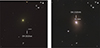 |
Fig. 1. Trichromy image from BVr single-filter observations with the Asiago Schmidt telescope a few days after the discoveries of SN 2020ue (left panel) and SN 2020nlb (right panel). The positions of these SN in their respective host galaxies are marked with white indicators. Courtesy of Giovanni Benetti (DFA, University of Padova). |
SN 2020nlb was discovered by ATLAS on 12 June 2020 (MJD = 59025.25) as a new object of magnitude o = 17.44 ± 0.08 mag (orange filter, Townsend et al. 2020) at the coordinates RA = 12:25:24.190, δ = +18:12:12.80. The host galaxy is NGC 4382, also known as M85, Fig. 1. The last non-detection by ATLAS was two days prior to discovery, at MJD = 59023.28. The spectroscopic confirmation as SN Ia in NGC 4382 was reported by the Nordic Optical Telescope Unbiased Transient Survey 2 (NUTS2) collaboration (Fiore et al. 2020). The galaxy has been classified as an S0 type galaxy (Trentham & Hodgkin 2002) and is located in the E cloud of the Virgo cluster (de Vaucouleurs 1961), opposite to the location of NGC 4636. Similar to NGC 4636, the distance modulus for NGC 4382 was estimated by CosmicFlows-3 to be μ = 31.00 ± 0.24 mag (Tully et al. 2016). This SN has already been studied by Sand et al. (2021) and Williams et al. (2024).
2.2. Photometry
Our photometric dataset includes data covering the UV and optical evolution of both SNe Ia from discovery to around 150 days post-peak brightness, obtained with various observational facilities. Optical observations were conducted at a nearly 1-day cadence near peak brightness, decreasing to a lower cadence during the slow-declining 56Co decay phase. However, a 70-day data gap exists for SN 2020nlb, starting approximately 40 days after peak brightness due to Sun proximity. Optical photometry in griz bands was obtained for both SN 2020nlb and SN 2020ue with the Panoramic Survey Telescope and Rapid Response System (Pan-STARRS) used in normal survey modes via the Young Supernova Experiment (YSE, Jones et al. 2021; Aleo et al. 2023; data accessed via YSE-PZ Coulter et al. 2022, 2023) and the Pan-STARRS search for kilonovae (McBrien et al. 2021). The Pan-STARRS1 (PS1) telescope is a 1.8-metre facility installed atop of the Haleakala on Maui, Hawaii, US (Chambers et al. 2016). It observes a 7.06-square-degree field with a grizy SDSS-like photometric filter system. PS1 data were processed in real-time at the University of Hawaii where transient sources were selected (Magnier et al. 2020), and later on, filtered and classified by the Transient Science Server at Queen’s University Belfast (Smith et al. 2020). The PS1 data for both the SNe presented here are shown in Fig. 2.
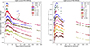 |
Fig. 2. Light curve evolution of SN 2020ue (left panel) and SN 2020nlb (right panel). Symbols denote data from different facilities (diamonds: Swift-UVOT; triangles: Copernico-AFOSC, NOT-ALFOSC (for SN 2020ue), and Pan-STARRS (for SN 2020nlb); squares: Swope and Thacher; circles: LCO; pluses: OASDG), with colours indicating filters. Both light curves have not been corrected for Galactic reddening. |
Additional optical and ultraviolet photometry of SN 2020ue and SN 2020nlb was obtained from multiple facilities. Optical observations were carried out with the Alhambra Faint Object Spectrograph and Camera (ALFOSC) at the Nordic Optical Telescope (NOT), the Asiago Faint Object Spectrograph and Camera (AFOSC) at the Schmidt 67/92 cm telescopes at Asiago, the Swope 1-metre telescope at Las Campanas, the Thacher 0.7-metre telescope, and the Las Cumbres Observatory (LCO) 1-metre network, using various combinations of uBVgri(z) filters. The data were reduced using dedicated employing point spread function (PSF) or forced photometry calibrated to the Sloan or Pan-STARRS systems. Ultraviolet observations were obtained with the Neil Gehrels Swift/UVOT and reduced with HEASOFT standard procedures. Additional BVR photometry for SN 2020nlb was collected with the Osservatorio Astronomico ‘Salvatore Di Giacomo’ (OASDG) 0.5-metre telescope and processed with an Astropy-based pipeline. A detailed description of the data reduction and analysis of each single dataset is provided in the Appendix A. The combined datasets provide well-sampled light curves from peak brightness through late epochs.
2.3. Spectroscopy
The entire spectral series, except for the high-resolution spectra obtained with the Lick/APF spectrograph, of both SNe discussed in this work are shown in Figs. 3 and 4. We obtained the spectral series covers a wide temporal range from −12 to 389 days for SN 2020ue, and from −16 to 273 days for SN 2020nlb. The phase was calculated with respect to the corresponding B-band maxima. The complete log of the spectroscopic observations is shown in Table B.1. The initial flux calibration was performed using spectro-photometric standard stars (Feige 34, Feige 56 and HR 3454, see also Appendix) observed each night. Thereafter, we photometrically ‘mangled’ (Hsiao et al. 2007) the spectra using available measured photometric data at each epoch.
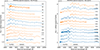 |
Fig. 3. Optical spectral series of SN 2020ue. Spectra were obtained with the Copernico 1.82m and Galileo 1.22m telescopes in Asiago, and the FLOYDS telescopes during the first 50 days of the SN evolution (left panel), and up to 390 days from B-band maximum (right panel). |
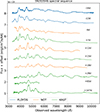 |
Fig. 4. Optical spectral series of SN 2020nlb. Spectra were obtained with NOT, FLOYDS, and KAST. |
Spectroscopic observations of SN 2020ue and SN 2020nlb were obtained using a wide range of instruments and facilities covering optical to NIR wavelengths. For SN 2020nlb, five epochs were acquired with NOT/ALFOSC, reduced with the PYNOT pipeline. Both SNe were also observed with the FLOYDS spectrographs on the LCO network of telescopes. Extensive optical coverage of SN 2020ue was obtained at the Asiago telescope with AFOSC and the echelle spectrograph. Additional spectra were collected with the Low-Resolution Imaging Spectrograph (LRIS) at the Keck telescope, Lick/Kast, and the Automated Planet Finder (APF) Levy spectrograph, providing both low- and high-resolution coverage. Near-infrared spectra of SN 2020ue were secured with IRTF/SpeX, and integral-field observations for both SNe were obtained using WiFeS at Siding Spring Observatory. Finally, one ultraviolet spectrum of SN 2020ue was obtained with Swift/UVOT. A detailed description of the data reduction and analysis of the spectral dataset obtained with each telescope – instrument pair is provided in the Appendix.
3. Photometric analysis
3.1. Peak brightness and intrinsic extinction
We analysed multi-filter light curves of SN 2020ue and SN 2020nlb using three methods: (1) the light curve fitter SNOOPY v2.5.3 (Burns et al. 2011), (2) the hierarchical Bayesian model BAYESN (Mandel et al. 2022; Ward et al. 2023), and (3) a custom Gaussian process (GP) regressor algorithm1 implemented in SCIKIT-LEARN (Pedregosa et al. 2011). Figure 2 shows multi-filter light curves of SN 2020ue and SN 2020nlb, both in days past B-band maximum, TB, max, determined using SNOOPY. This Python package analyses and fits SN Ia light curves in various photometric filters using templates and light curve behaviour models. Prior to fitting, SNOOPY corrects SN light curves for Galactic extinction and performs K-corrections based on Hsiao et al. (2007). We estimated the B-band maximum using the max-model and the colour-stretch parameter sBV, a dimensionless, normalised parameter representing the epoch past maximum light when the B − V colour curve peaks (Burns et al. 2014). We also employed the B-band decay rate, Δm15(B), noting that our B-band maximum results are consistent with those from Sand et al. (2021) within uncertainties.
We used the entire Swift-UVOT dataset combined with Pan-STARRS gri data for SN 2020nlb, and photometric data from NOT, Copernico 1.82m and Schmidt 67/92 Asiago telescopes for SN 2020ue to obtain light curve parameters (Table 1). Using the max-model, we obtained the following results (with results for EBV-model2 and Δm15 decay rate parameter also reported in Table 1 for extinction estimation and SN bolometric light curve construction). For SN 2020ue, the B-band light curve peaks at Bmax, 20ue = 11.982 ± 0.011 mag on TB, max, 20ue = 58873.25 MJD with colour-stretch parameter sBV = 0.735 ± 0.008. For SN 2020nlb, the B-band light curve peaks at Bmax, 20nlb = 12.164 ± 0.094 mag on TB, max, 20nlb = 59042.12 MJD with colour-stretch parameter sBV = 0.923 ± 0.009.
Results of the light curve fits made with SNOOPY.
We also employed a dedicated GP regressor algorithm to fit B- and V-band light curves separately, estimating Δm15 without SN templates. Our GP kernel comprised three components: (1) a constant scaling kernel, (2) a rational quadratic kernel with length scale l = 3 and scale mixture parameter α = 3/2, and (3) a white kernel representing white noise with variance σ2 = 1. This method suits SN light curves with a temporal cadence near the length scale l. Similar to SNOOPY, we corrected for Galactic extinction and applied K-corrections before fitting. Light curve parameters were measured using the predictor properties of the GP regressor function, including the stretch-colour sBV.
In Fig. 5, we display the best-fit results for both SNe obtained using the GP method from SNOOPY. In Appendix Fig. B.4, we show the best-fit results using the GP regressor method developed in this work. We find the GP method produces a very good agreement with the SNOOPYmax-model fitting results obtained using the LCO light curve data for SN 2020ue, and for SN 2020nlb using the OASDG and the Thacher telescope data (see Appendix Fig. B.6 and Table B.3).
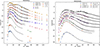 |
Fig. 5. SNOOPY fits (black curves) to Swift-UVOT and Pan-STARRS gri data of SN 2020ue (left panel) and SN 2020nlb (right panel). The fits were obtained with the max-model light curve model function and the sBV stretch-colour parameter. |
Our choice of the max-model option in SNOOPY is based on the estimation of the stretch-colour parameter sBV and the cosmological application of the fit results. However, this model does not account for host galaxy extinction, focusing instead on fitting the maximum magnitude of each filter light curve (Burns et al. 2014). SNOOPY offers an alternative approach: fitting the EBV-model2 before max-model, which includes an additional free parameter for inferring host galaxy extinction, E(B − V)host, and provides an estimate of the distance modulus μ. The extinction curve parameter value for the host galaxy is fixed to RV = 3.1. We obtained near-zero extinction for SN 2020ue and a significant extinction value of E(B − V)20nlb = 0.113 ± 0.009 mag for SN 2020nlb (with 0.060 mag systematic errors for both cases).
We used BAYESN for comparison, which models the continuous optical-to-NIR spectral energy distribution (SED) of SNe Ia over time with intrinsic functional principal components scaled by dust extinction parameters. This latent reddened SN SED reconstruction enables us to quantify dust extinction (Fitzpatrick 1999) (parametrised by total extinction in the V band, AV) and to derive the intrinsic SED distance modulus. Fig. B.1 presents BAYESN model-fits for SN 2020nlb and SN 2020ue photometric datasets (as used with SNOOPY in Fig. 5), including a corner plot of inferred parameters: distance modulus μ, V-band absorption AV, and light curve shape θ (Mandel et al. 2022).
Regardless of the fitting methods and models (SNOOPY models, BAYESN), the inferred distance to SN 2020nlb is slightly lower than that of SN 2020ue. Individual distance estimates for both SNe, inferred using both methods, agree within statistical uncertainties. For SN 2020nlb, our findings align with Williams et al. (2024), who used SNOOPY’s EBV-model2 for distance determination. Similar results emerge when using PS1 and Swift data fitting results alone (Fig. 5).
The extinction in the V-band parameters obtained with BAYESN suggests an environment for SN 2020nlb that is more attenuated (AV = 0.29 ± 0.04 mag) than for SN 2020ue (AV < 0.06 mag, 95% cl.), although still in agreement with the results obtained using SNOOPY. We also used the empirical relation between the B − V colour at the SN maximum and the decay rate parameter Δm15(B) proposed by Phillips et al. (1999). Adopting the B- and V-band maximum magnitudes resulting from the SNOOPYmax-model fits without prior extinction correction, we obtain E(B − V)20ue = −0.049 ± 0.023 mag and E(B − V)20nlb = 0.140 ± 0.010 mag. This is consistent with the results from our other fitting methods and demonstrates that indeed, SN 2020ue is not affected by host galaxy dust extinction. All results of our SNOOPY analysis are listed in Table 1, where all the reported magnitudes have been corrected for Galactic extinction, E(B − V)20ue, MW = 0.024 mag and E(B − V)20nlb, MW = 0.026 mag.
3.2. Bolometric light curves
Fig. B.2 displays estimated bolometric light curves for SN 2020ue and SN 2020nlb, constructed using SNOOPY’s BOLOMETRIC function and DIRECT method, following Gall et al. (2018). UV-band light curves were built using GP spline functions within SNOOPY. A quasi-bolometric light curve was created through direct flux measurements from observed epochs, with spectral energy distributions interpolated via a ‘spline’ fit method. Rayleigh-Jeans extrapolation based on UV and optical fluxes was used for the NIR range. We assumed zero host extinction for SN 2020ue (Sect. 3.1), while E(B − V) = 0.113 mag was used for SN 2020nlb based on the EBV-model2 fit (Table 1). The bolometric flux was placed on the absolute luminosity scale using distance moduli from SNooPy (Table 1): μ = 31.139 mag for SN 2020ue and μ = 30.961 mag for SN 2020nlb. Light curve uncertainties were determined by iterating the process 50 times and averaging the results.
We employed the same GP regressor algorithm and kernel as in Section 3.1 to determine the peak bolometric luminosity,  . For SN 2020nlb, the bolometric light curve peaked at MJD
 days, occurring 0.41 ± 0.17 days before TB, max with a luminosity of
  erg s−1. For SN 2020ue, the bolometric light curve peaked at MJD
 days, 0.91 ± 0.12 days before TB, max, with a luminosity of
 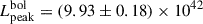 erg s−1.
3.3. SN explosion and rise-time to peak brightness
For SN 2020nlb, the early high-cadence Pan-STARRS g- and r-band observations, beginning 16.2 days before maximum light, together with stringent ATLAS upper limits obtained two days before discovery, provide a precise constraint on both the explosion time and the rise time. However, for SN 2020ue, our data coverage begins about 5 days later, at −11.9 days in B and V bands obtained from the Copernico 1.82m telescope at the Asiago Observatory. Thus, for SN 2020ue, we can only provide an estimate.
We explored the applicability of an expanding fireball model for the very early emission of both SNe, where the SN luminosity evolution with time is proportional to the square of the explosion time, L ∝ t2 (Riess et al. 1999). This rise-time depends on factors such as the synthesised 56Ni amount (Arnett 1982; Shigeyama et al. 1992; Hoeflich et al. 1993) and its distribution within the ejecta. Progenitor WD metallicity, influencing the binding energy of the WD and ejecta expansion velocities (Höflich et al. 2010), is another factor affecting SNe Ia rise-times. Distinct rise-times of B-band light curves have been determined for various SNe Ia sub-types (Riess et al. 1999; Ganeshalingam et al. 2011; González-Gaitán et al. 2012; Firth et al. 2015). Recently, a t2 evolution was confirmed in a volume-limited sample of ZTF SNe Ia (Miller et al. 2020) but is not universally observed (Fausnaugh et al. 2023).
Summary of distance moduli (in magnitudes) for the SN host galaxies.
The fireball phase typically lasts about a week post-SN Ia explosion, when the flux reaches 40−50% of the SN Ia peak brightness (Miller et al. 2020). For SN 2020nlb, we analysed all g- and r-band Pan-STARRS data between the last non-detection from ATLAS and up to 10 days after and fitted them using a power law model, L ∝ tγ. Our analysis shows that a power-law index of γr = 2.38 ± 0.02 (statistical uncertainty only) effectively describes the initial rise to peak brightness. However, extrapolating the best-fit result to earlier times contradicts existing ATLAS upper limits (Fig. 6), indicating an explosion time roughly 2 days before the last ATLAS non-detection, suggesting a discrepancy between inferred event onset and observational constraints. For the g band, we obtained γg = 2.74 ± 0.02 (stat. unc.), with the extrapolation consistent with non-detections at earlier times. Our findings are compatible with those of Williams et al. (2024), making SN 2020nlb a ‘single SN’ Ia in the Hoogendam et al. (2024) rising light curve classification scheme.
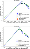 |
Fig. 6. Pan-STARRS g- and r- band light curves of SN 2020nlb (upper panel) and Copernico 1.82m B- and V-band SN 2020ue (lower panel), computed using the procedure outlined in Sect. 3.2. The dashed lines represent the best-fit obtained with a power-law model for the early light curve evolution (González-Gaitán et al. 2012). The most stringent ATLAS upper limit is indicated by an orange triangle, while an additional upper limit reported by Sand et al. (2021) 1.3 days later is marked by a red symbol at the time of the ATLAS observation. For SN 2020ue, the best-fit model extrapolation for the r band is consistent with these flux upper limits. |
An alternative approach to estimating the explosion time involves analysing the evolution of the SN ejecta’s photospheric velocity, well represented by the blueshift minimum of the Si II 6355 Å absorption line. In a polytropic ejecta structure with an index n = 3, the photospheric velocity evolution follows a power-law decay before peak brightness, with a power-law index of α = 0.22 ± 0.02 (Piro & Nakar 2014). We measured the blueshifted velocity of the Si II 6355 Å line for all available epochs around peak brightness for both SNe, as detailed in Section 4.2. We then applied a Levenberg-Marquardt algorithm for non-linear fit minimisation, as implemented in the scipy Python package, to fit the data series to a power-law model: v(t) = v0 × (t − texp)−0.22. Using this analysis, we determined the explosion time for both SNe via the Si II 6355 Å line’s photospheric velocity evolution. For SN 2020nlb, our results indicate an explosion time of MJDexpl = 59019.4 ± 1.2, occurring 2.6 days before the last epoch of non-detection by ATLAS. This estimate aligns with the results obtained before using the power-law fit of the rising light curve. For SN 2020ue, the explosion time is MJDexpl = 58853.9 ± 1.1, consistent with non-detections and the early light curve analysis.
Deviations from the fireball value of γ = 2 could have different explanations. Possible origins include enhanced circumstellar medium (CSM) density near the WD progenitor (Moriya et al. 2023), which can enhance and redden the early light curve, or an excess of 56Ni in the SN ejecta’s outer region (Magee & Maguire 2020; Ni et al. 2023a). An early red colour for SN 2020nlb is indeed evident in the B − V evolution diagram of Fig. 8 (see also Sect. 3.3). Early red excess has been observed in various SNe Ia (Dimitriadis et al. 2019; Wang et al. 2021, 2024; Ni et al. 2022). In particular, SN 2020nlb shows strong similarities with early-red events such as SN 2021aefx (Ni et al. 2023b) and KSN-2017iw (Ni et al. 2025), see Fig. 8. For SN 2020ue, the paucity of data from the very early stages of the event prevents pinpointing the explosion time. Nevertheless, as shown in Figure 6, the best-fit results for the power-law model reveal steep power-law indices for both B and V light curves. Extrapolations to earlier epochs are consistent with the constraints provided by our ATLAS non-detection.
3.4. The ejected mass of 56Ni
Type Ia SN emission is primarily driven by heating from radioactive 56Ni decay, synthesised in the thermonuclear explosion (Pankey 1962; Truran et al. 1967; Colgate & McKee 1969). Under simple initial assumptions, analytical models, such as the Arnett (Arnett 1982) model, were developed to infer key physical properties, such as the ejected 56Ni mass, MNi. Widely used in the literature, Arnett’s model measures synthesised 56Ni in type I SNe from the time of the bolometric peak luminosity, assuming: (1) time-independent radiation energy density, partially limiting parameter estimate accuracy (Pinto & Eastman 2000), and (2) initial spherical symmetry. Recently, Khatami & Kasen (2019) presented an updated relation between bolometric peak luminosity and timing in SNe Ia, considering the heating source’s spatial distribution and non-constant opacity effects on the light curve. They introduced β, quantifying the degree of 56Ni mixing within the ejecta and how spatial distribution varies among SN types. For SNe Ia, β = 1.6 was estimated. We applied both methods to infer the 56Ni mass of SN 2020nlb and SN 2020ue, using the updated formulation of Khatami & Kasen (2019) from Woosley et al. (2021).
Some SNe Ia discoveries occur shortly after the supernova explosion (Nugent et al. 2011; Li et al. 2011b; Hosseinzadeh et al. 2017; Ashall et al. 2022). For SN 2020nlb, both early light curve fitting and photospheric velocity methods suggest an explosion epoch approximately 2.6 days before the most constraining ATLAS upper limits. To validate these estimates, we used the analytical formulation for Type I supernova bolometric light curve evolution from Valenti et al. (2008). This model relies on such parameters as total ejected mass, fraction of synthesised 56Ni, and ejecta kinetic energy, formulated in terms of photospheric velocity at peak brightness (Valenti et al. 2008; Lyman et al. 2016), provided as a fixed prior in our analysis. This method also enables estimation of the explosion time. Additionally, we accounted for gamma-ray leakage correction, caused by gamma-ray photons from heavy element decay powering SN emission (Clocchiatti & Wheeler 1997). Free parameters in this model include optical opacity K and gamma-ray opacity kγ. Gamma-ray leakage effects become noticeable approximately a week after the SNe I bolometric light curve peak. Our model only considered gamma-ray leakage from 56Co decay and positron annihilation, as high-energy photons from positron kinetic energy significantly impact SN light curves at > 200 days post-explosion (Clocchiatti & Wheeler 1997; Tucker et al. 2022). We performed a best-fit analysis of the bolometric light curve using the described analytic model, with final results shown in Table 3 and Fig. B.3.
Physical properties from best-fit analysis of bolometric light curves of SN 2020nlb and SN 2020ue using using the analytical model.
The analytical Arnett model yields an SN 2020nlb explosion time consistent with the ATLAS upper limits, MJDexpl = 59026.13 ± 0.56. Similarly, SN 2020ue’s explosion epoch is MJDexpl = 58858.77 ± 0.58, aligned with the ATLAS non-detection and previous estimates (Sect. 3.3). For 56Ni mass, we obtain M56Ni = 0.40 ± 0.10 M⊙ for SN 2020nlb and M56Ni = 0.36 ± 0.11 M⊙ for SN 2020ue. These 56Ni masses are consistent within uncertainties and indicate that the self-similar energy density assumption by Arnett (1982) is suitable for modelling normal SNe Ia (Blondin et al. 2013). Our findings align with literature expectations (e.g. Stritzinger et al. 2006; Kasen & Woosley 2007; Dhawan et al. 2018), where SNe Ia with lower Δm15 values exhibit larger ejected 56Ni masses. As the bolometric peak luminosity of SNe Ia is driven by the synthesised 56Ni amount, this relation offers an alternative interpretation of the Phillips relation (Stritzinger et al. 2006). Fig. 7 shows the distribution of 56Ni mass versus Δm15 for our studied SNe, alongside other SNe Ia (Dhawan et al. 2018). Both SN 2020ue and SN 2020nlb occupy the region of normal SNe Ia. The lower right corner hosts SNe Ia with low 56Ni mass (< 0.3 M⊙), including transitional events such as SN 2007on (Gall et al. 2018) and fast-decliner SNe such as SN 2005ke, SN 2007mr, and SN 2007ax (Dhawan et al. 2018).
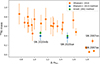 |
Fig. 7. Distribution of 56Ni masses for SN 2020nlb and SN 2020ue as a function of Δm15 determined using both the Khatami & Kasen (2019) method (blue data) and the Arnett (1982) analytical model (green data). For comparison, we include the Arnett model results (orange data) for the SNe Ia sample from Dhawan et al. (2018). The locations of the transitional and fast-declining events SN 2007on (Gall et al. 2018) and SN 2007ax (Kasliwal et al. 2008) are highlighted. |
3.5. Colour evolution
Fig. 8 presents the B − V colour evolution of SN 2020nlb and SN 2020ue compared to nearby calibrator SNe Ia (Riess et al. 2016; Khetan et al. 2021). The B − V evolution for SNe was computed using SNooPy’s dedicated built-in function, requiring a defined light curve fit model and decay rate parameter. Fig. 8 also includes the colour evolution of transitional high-Δm15 SNe Ia SN 2007on and SN 2011iv (Gall et al. 2018, see Sect. 1). Type Ia SNe typically exhibit their bluest colours ∼ − 10 days before B-maximum, then abruptly turn redder, reaching the reddest colours ∼10 to ∼40 days post-maximum. Subsequent evolution features a linear decline towards bluer colours, with a similar decline rate for all SNe Ia. Termed the ‘Lira-law’ (Lira 1996), this behaviour has been employed to estimate host galaxy extinction (Phillips et al. 1999; Folatelli et al. 2010), assuming SNe following the Lira-law (Fig. 8’s dashed black line) experience low to zero extinction. Thus, colour offsets from the Lira-law can be attributed to host galaxy extinction.
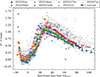 |
Fig. 8. Temporal (B − V) colour evolution, featuring SN 2020ue (blue stars) and SN 2020nlb (orange stars), along with a sample of nearby SNe Ia taken from Riess et al. (2016) and Khetan et al. (2021) (grey data), transitional SNe Ia (SN 2007on: Pink triangles; SN 2011iv: brown triangles, Gall et al. 2018), and early-time red SNe Ia (KSN 2017iw: violet squares; SN 2018aoz: green squares; SN 2021aefx: red squares, Ni et al. 2023b, 2025). The dashed black line indicates the Lira-law regime (Phillips et al. 1999). |
Around B-band maximum, SNe Ia colours are confined within a small B − V colour range, while larger colour variations emerge at later epochs (Fig. 8). Unfortunately, SN 2020nlb data beyond 40 days past B-band maximum are unavailable due to observational constraints. However, our data indicate that SN 2020nlb peaked at B − V ∼ 1.45 mag around 25 days post-B-band maximum, confirming light curve fit results (Sect. 3.1, Table 1) that SN 2020nlb experiences significant host galaxy extinction.
SN 2020ue’s colour evolution is comparable to transitional SNe Ia SN 2007on and SN 20211iv, attaining B − V peak magnitude ∼17−20 days post-B-band maximum. Intriguingly, SN 2020ue exhibits the bluest colour at B-band maximum of all highlighted transitional and fast-declining SNe in Fig. 8. However, its B − V colour evolution past the B − V peak in the Lira-law regime (30−90 days) aligns with SN 2007on. As discussed in Sect. 1, B − V colour variations may be intrinsic, originating from such physical differences in the progenitor WD system as the distinct central densities of progenitor WDs (e.g. Hoeflich et al. 2017; Gall et al. 2018) or explosion asymmetries (e.g. Maeda et al. 2011; Foley & Kasen 2011); however, they can also be extrinsic, due to such properties of the birthplace environment as metallicity or dust (Wang et al. 2013, 2019).
4. Spectral evolution
Both SNe display characteristic spectral features of SNe Ia (see e.g. Morrell et al. 2024). Our extensive spectral coverage, particularly near the SN explosion, enables the analysis of the absorption line evolution from ∼−10 days to peak brightness. Key insights can be gleaned from line velocity and intensity evolutions, revealing information on the ejecta’s stratified composition and unburned elements such as carbon and oxygen (though oxygen is also a carbon-burning product). Although oxygen is commonly observed in optical SN Ia spectra, detecting carbon remains challenging. Carbon presence in optical SN Ia spectra has been reported in early (< 10 days pre-peak brightness) spectra of numerous (∼30−40%) SNe Ia (see e.g. Branch et al. 2003; Thomas et al. 2007, 2011; Parrent et al. 2011; Folatelli et al. 2012; Silverman & Filippenko 2012; Maguire et al. 2014; Dutta et al. 2021; Zeng et al. 2021, and references therein). Detecting carbon signifies incomplete burning, with crucial implications for interpreting the progenitor star’s nature and the mechanisms driving element mixing in the ejecta (Nomoto et al. 1984; Iwamoto et al. 1999; Folatelli et al. 2012).
The primary optical feature C II 6580 Å often blends with the prominent Si II 6355 Å line, making line identification challenging (Folatelli et al. 2012). When the Si II line is intense, the upper level (3p–3d) C II 7234 Å transition can be detected as a faint line. Since unburned elements only persist in the stratified ejecta’s outermost layers, C II 6580 Å shows higher velocities than other absorption lines at similar epochs, such as the nearby Si II 6355 Å line (Fisher et al. 1997; Mazzali 2001; Heringer et al. 2019). However, carbon has also been detected at lower velocities in some instances (Maguire et al. 2014), implying that carbon often blends with the silicon line’s red wing in many high- and normal-velocity SNe Ia (see Parrent et al. 2011; Folatelli et al. 2012 for discussion). Based on this, we identify possible C II 6580 Å in the earliest spectrum (phase −12 d) of SN 2020ue, observed as a faint dip at the Si II 6355 Å line’s red wing edge. This feature remains visible with reduced intensity until −4 days, displaying a similar expansion velocity (∼15 000 km/s) to the Si II line (Fig. 9). Conversely, neither C II 7234 Å nor C II 6580 Å is visible in early SN 2020nlb spectra. This is unsurprising, as C I detection is more likely in SNe Ia with bluer peak colours, faster-declining light curves, and lower Si II velocities (e.g. Thomas et al. 2011; Silverman & Filippenko 2012; Folatelli et al. 2012). Strong C I detection in pre-maximum NIR spectra of transitional SNe Ia has been noted (e.g. Höflich et al. 2002; Hsiao et al. 2015; Wyatt et al. 2021), and for more luminous, normal SNe Ia, a C I ‘knee’ feature may be present (e.g. Hsiao et al. 2013; Hoogendam et al. 2025). Given this, the early C II detection and absence of carbon features at day −5 in optical and near-IR wavelengths argue against a possible ‘transitional’ nature for SN 2020ue.
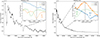 |
Fig. 9. Spectrum of SN 2020ue at −12 days (left panel) and −5 days (right panel). Left inset: Radial velocity spectrum centred on the Si II 6355 Å, C II 6580 Å, and C II 7234 Å. Right inset: Carbon lines in the optical and NIR spectra. The grey strip marks the epoch expansion velocity of the Si II 6355 Å line, as measured with spextractor. |
4.1. Pseudo-equivalent widths
We quantified spectral properties by measuring the pseudo-equivalent width (pEW), Doppler velocity, and line depth of prominent absorption features using a modified version of the publicly available code Spextractor (Papadogiannakis 2019; Burrow et al. 2020). It employs GP regression to fit the analysed spectrum, then estimates pEWs for given absorption lines by identifying their flux minima (see Burrow et al. 2020 for details). We focused on absorption lines commonly observed in SN Ia spectra, including Ca II H&K, Si II 4130 Å, Mg II 4481 Å, Fe II 5062 Å triplet, S II 5468/5624 Å doublet, Si II 5972 Å, Si II 6355 Å, and O I 7775 Å. Some lines blend with fainter transitions of other elements (e.g. Si II 4130 Å blends with Ti II 4200 Å around peak brightness, typically observed for fast-decliner events, Taubenberger 2017).
We included an essential constraint in the prior distributions of each absorption line considered in the fit: all lines should have a similar offset for the low and high-velocity range defining each absorption line. This is particularly applicable to absorption lines not predominantly affected by blends up to a few days past peak brightness (e.g. Si II 5972 Å begins to be affected by Na I five days post-peak brightness), while for multiplets such as Fe II, we considered a wide range due to multiple components. To establish absorption line boundaries, we considered the blue and red wavelength maxima of the absorption trough for Si II 6355 Å as it is least affected by blending with other absorption lines. This accounts for the weak C II 6580 Å presence in SN 2020ue, which minimally impacts the pseudo-continuum and pEW value. Fig. B.5 demonstrates the best-fit result from our Spextractor for SN 2020ue’s −1 day spectrum. Our analysis focuses on spectra from the early rising phase up to approximately 8 days post-B-band peak maximum. Table B.2 summarises the measurements for SN 2020ue and SN 2020nlb.
Absorption line properties around peak brightness in SNe Ia have been used to identify common patterns (Nugent et al. 1995; Benetti et al. 2005; Bailey et al. 2009; Wang et al. 2009; Morrell et al. 2024). We focus on the Branch et al. (2006) classification scheme (‘Branch-classification’), which categorises SNe Ia into four spectroscopic sub-classes based on the pEWs of Si II 5972/6355 Å lines: cool (CL), core normal (CN), shallow silicon (SS), and broad line (BL). To assess how SN 2020ue and SN 2020nlb fit within this classification, we utilise the Burrow et al. (2020) dataset for comparison, as spectroscopic properties were measured using the same method as in our work. We consider pEW values for SN 2020ue from the −1 day spectrum, and for SN 2020nlb, the closest spectrum to B-band peak available at −6 days. Fig. 10’s top panel displays our two SNe’s pEW measurements in the ‘Branch-plot’. Additional SNe Ia observed in late-type and early-type galaxies are included as they were employed as Cepheid (Riess et al. 2016) and/or SBF (Khetan et al. 2021) calibrators of SN luminosity relations.
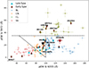 |
Fig. 10. Branch spectroscopic classification scheme. SNe Ia classes are shown in various colours: SS, red; BL, blue; CL, green; and CN, orange. The dashed lines separate these regions (Phillips et al. 2022). SNe Ia in late-type (Riess et al. 2016, Cepheid calibrators) and early-type galaxies (Khetan et al. 2021, SBF calibrators) are shown as blue triangles and brown diamonds, respectively. SN 2020ue and SN 2020nlb are highlighted as black and red stars. Transitional and fast-declining SNe Ia, such as SN 1991bg, 1997cn, 2007on, 2011iv, and 2015bo, as well as early red events, such as 2018aoz and 2021aefx, are also included (Gall et al. 2018; Hoogendam et al. 2022; Ni et al. 2023a,b). |
Firstly, we observe that SN 2020ue and SN 2020nlb are situated within the CN and BL regions, respectively. This positioning aligns with most calibrator SNe included in this analysis, distributed between these two classes. A few exceptions exist, i.e. SNe Ia belonging to other spectral classes, which nonetheless were included in calibrating samples. These include SN 1991T, and the transitional events SN 2007on and SN 2011iv. SN 1991T, located at the extreme edge of the SS sub-class, is the prototype of a subclass of SNe Ia characterised by high-luminosity and slowly-evolving light curve behaviour, accompanied by pre-maximum weak Si II and strong Fe II lines (Filippenko et al. 1992b; Phillips et al. 1992). The two transitional events were considered SBF SN calibrators in Khetan et al. (2021) and represent the sole calibrating SNe Ia within the CL sub-class, which also contains the fast-decliner prototype, SN 1991bg (Leibundgut et al. 1993). Type Ia supernovae in the CL-class are located in the region where we find type Ia SNe characterised by a very intense Si II 5972 Å line compared to those in other spectroscopic sub-classes. Cool SNe photometrically differ from most SNe Ia in other sub-classes, becoming evident when examining the distribution of Si II 5972 Å pEW and R(Si) = pEW(Si II 5972)/pEW(Si II 6355) relative to Δm15. Both the Si II 5972 Å pEW and Si II pEW line ratio consistently demonstrate a linear relationship with SNe Ia light curve decay rates across various SN Ia samples (Hachinger et al. 2006; Taubenberger et al. 2008; Hachinger et al. 2008; Blondin et al. 2012; Zhao et al. 2021). The tightest correlation emerges for Si II 5972 Å pEW (see Fig. 10’s lower panel), causing a clear separation of CL SNe Ia from BL, CN, and SS sub-classes in the upper-right region of Fig. 10 (middle and lower panels). This region is characterised by high Si II 5972 Å pEWs and elevated Δm15 (> 1.5) values. This distinction is noticeable for transitional SN 2007on and SN 2011iv, and fast-decliner SN 1991bg, markedly separated from other calibrator SNe. Intriguingly, despite SN 2020ue being a ‘border-line’ event with Δm15 values close to SN 2011iv and a strikingly similar colour evolution as SN 2007on, its spectroscopic behaviour differs from transitional events. Conversely, SN 2020nlb exhibits typical spectroscopic evolution of normal SNe Ia.
4.2. Time-resolved analysis
To further explore the temporal spectroscopic behaviour of SN 2020ue and SN 2020nlb, we analyse selected spectroscopic features as a function of time. Specifically, we computed velocities and pEWs of the two Si II transitions at λλ5972 and 6355 Å using spextractor. We compare our results with a similar analysis of SNe 2007on and 2011iv, utilising photometry and spectroscopy from Gall et al. (2018). Our measurements align with the results reported by Burrow et al. (2020) for SN 2007on and SN 2011iv. Figure 11 places the results obtained from our analysis, the expanding velocity for the Si II 6355 Å line and the pEW of the Si II 5972 Å, in perspective to the average trend of the same quantities obtained by the analysis of 247 SNe Ia from the Berkeley Supernova Ia Program (Stahl et al. 2020). Our decision to use the expansion velocity of Si II 6355 Å and the pEW value of Si II 5972 Å is motivated by the fact that Si II 6355 Å is easily saturated in SNe Ia spectra (Hachinger et al. 2008; Zhao et al. 2021), while Si II 5972 Å is not. Line blending is another concern; Si II 5972 Å is minimally affected, except for a small C II contribution at pre-B-band maximum epochs (see Sect. 4). However, Si II 5972 Å becomes strongly affected by other transitions such as S II at epochs ∼10 days after B-band maximum (Stahl et al. 2020). This is evident in Fig. 11, where pEW(Si II 5972 Å) values begin increasing at epochs > 5 days past B-band maximum. We also notice that in post-peak epochs, the increasing intensity of the emission in P-Cygni profiles starts to affect the measurement of pEWs.
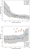 |
Fig. 11. Upper panel: Blueshifted velocity evolution inferred using spextractor on early spectra of SN 2020ue (blue), SN 2020nlb (orange), as well as transitional SNe SN 2011iv (green) and SN 2007on (red). The grey line and shaded region represent the average trend from the 247 SN sample in Stahl et al. (2020), analysed using the same method. Lower panel: Evolution of the pEW of the Si II 5972 Å line compared to the average trend reported in Stahl et al. (2020). |
Our analysis reveals two key findings. First, no significant difference is observed between SNe velocity evolution analysed here and the average trend reported by Stahl et al. (2020). While SN 2007on matches SN 2020ue evolution, SN 2020nlb displays lower velocities earlier, becoming consistent with the general trend around the B-band maximum. Second, and most intriguingly, transitional SNe display significantly higher values (above Stahl et al. 2020 average) for Si II 5972 Å pEW, as expected for CL SNe. In contrast, SN 2020ue aligns with the average trend exhibited by normal SNe Ia, indicating that SN 2020ue more closely resembles normal SNe Ia than extreme 1991bg-like events. We note that Si II 5972 Å pEW values in SNe Ia remain relatively constant from ∼−12 days to ∼5 days relative to B-band maximum. This finding implies that at epochs before peak brightness, SNe Ia with pEW values deviating from the average trend in Fig. 11 can be identified as part of the CL sub-class, and then classified as either transitional or fast-declining events, which constitute most events within this sub-class.
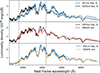 |
Fig. 12. Spectral modelling and comparison between SN 2020ue and SN 2011iv. Top panel: UV and optical spectra observed at a similar epoch (about six days before peak brightness) for SN 2020ue (black) and SN 2011iv (blue, Gall et al. 2018). Middle panel: Results from the TARDIS simulations (red curve) for the spectrum of SN 2020ue (black). Lower panel: Results from the TARDIS simulations (orange curve) for the SN 20211iv spectrum (black). The region between the two dashed grey lines corresponds to the wavelength range considered for the minimisation of the root-mean-square value (see Sect. 4). |
4.3. Spectral synthesis analysis
The differing temporal evolution of the Si II 5972 Å line in SN 2020ue and transitional SNe Ia SN 2007on and SN 2011iv (Fig. 11) suggests inherent physical differences in the ejecta evolution. The three SNe exhibit similar absorption line evolution in the red wavelength range (λ > 5000 Å). However, substantial differences emerge at blue wavelengths, where flux level variations are complex due to metallicity, line blanketing, and other physical effects such as ionisation (e.g. Sauer et al. 2008; Foley et al. 2012; Mazzali et al. 2014; Pan et al. 2015). Near peak brightness, stronger absorption troughs are observed for transitional SNe than for SN 2020ue. Interestingly, the observed differences in the UV spectral range align with our results from the colour evolution analysis (Sect. 3 and Fig. 8), revealing bluer colours for SN 2020ue around B-band maximum than SN 2007on, SN 2011iv, and most other SNe in Fig. 8. This suggests a physical origin for the observed spectral differences rather than a geometrical or viewing angle effect (e.g. Kromer & Sim 2009).
To further examine the identified spectral discrepancies among these SNe, we employed spectral synthesis analysis using the Monte Carlo radiative transfer code TARDIS (Kerzendorf & Sim 2014; Kerzendorf et al. 2018). TARDIS can simulate synthetic spectra directly compared to observed SN Ia spectral emission based on specific assumptions: (1) ejecta density distribution, (2) abundance composition, and (3) bolometric SN luminosity. These quantities were analysed at each epoch. We assumed a homologous velocity field and spherically symmetric ejecta. The abundance profile was not fixed at the start of our analysis. Instead, it varied according to the best-fit synthetic spectrum simulating the observed emission. This approach is valid as we focused on a single spectral epoch (see below), assuming uniform element abundance within the SN shell boundaries for the line-forming region. With a continuous spectral series, one could reconstruct a comprehensive radial abundance pattern for the SN ejecta (e.g. Stehle et al. 2005; Mazzali et al. 2008, 2014; Ashall et al. 2016, 2018). Here, we concentrate on the spectral analysis of SN 2020ue and SN 2011iv, for which we have UV and optical spectral coverage at a similar epoch (six days before B-band maximum), emphasising spectral differences around their peak brightness spectra.
We directly estimated the photosphere’s temperature from the best value obtained for the ejecta’s inner radius at each spectral epoch and the corresponding luminosity used in the simulation. We adopted the Branch et al. (1985) W7 density model for the density distribution, along with the nebular ionisation and dilute local thermodynamic equilibrium (LTE) excitation mode for the plasma configuration, and the downbranch line interaction method. To select the best-fit result, we estimated the root mean square from the SN luminosity and TARDIS simulation in the 2800 Å to 4200 Å wavelength range. This range was chosen for two reasons: (1) to maximise the match between the TARDIS simulation and observed data in the near-UV range, and (2) to avoid the blackbody approximation at longer wavelengths, which typically overestimates the spectral continuum at λ > 5500 Å. For more details on model parameters and the code, please refer to Kerzendorf & Sim (2014).
Fig. 12 showcases the analysis results. The TARDIS simulation accurately fits the entire spectral region of SN 2020ue, except for the bright emission features at 4000 Å, which are underestimated in flux by about 10%. Similar results are obtained for SN 2011iv, although the simulation does not reproduce the continuum at red wavelengths precisely. Notably, the Si II 5972 Å line is not accurately reproduced, likely due to the assumed uniform abundance distribution in the shell region. The main physical properties and abundance composition obtained from the best-fit model are presented in Table 4. We observe that the photosphere is at similar radii (in the homologous expansion approximation, radial velocity serves as a scaled proxy of the distance from the centre) in both SNe, while the outer boundary is at higher (∼1600 km/s) values in 2011iv. The temperature is similar in both SNe. The most significant difference in our analysis is that the SN ejecta is more enriched with Fe-peak elements in 2011iv, whereas IMEs exhibit nearly identical abundance values to those seen in SN 2020ue. SN 2011iv’s spectral behaviour was also analysed by Ashall et al. (2018). The availability of a spectral series covering a large time interval enabled Ashall et al. (2018) to perform an abundance tomography analysis, reconstructing the abundance pattern throughout the entire SN ejecta. The density distribution used in Ashall et al. (2018) differs from the W7 model employed here, leading to differing results from our TARDIS analysis. Ashall et al. (2018) found lower abundances for oxygen and iron and slightly higher values for Si, Mg, and Ni. However, Ashall et al. (2018) also concluded that SN 2011iv might have a high central density (Ashall et al. 2016). This finding suggests that transitional and fast-declining SNe may originate from progenitors with distinct properties compared to normal SNe Ia.
Physical properties and element abundances obtained from the TARDIS simulation of day −5 spectra of SN 2020ue and day −6 of SN 2011iv.
4.4. The nebular phase
Approximately 200 days after the SN explosion, the SN ejecta became optically thin, allowing scrutiny of the interior region. The spectrum during this nebular phase features emission lines from newly synthesised elements reflecting the ejecta’s velocity distribution. Analysing SN emission features in this phase can provide valuable insights into physical properties of the SN event, including MNi synthesised in the thermonuclear explosion, total ejected mass, and clues about the (a)symmetry of the explosion. Spectral synthesis methods or emission line relations can yield quantitative measures (Kuchner et al. 1994; Mazzali et al. 1998; Stritzinger et al. 2006; Mazzali et al. 2007; Graham et al. 2017; Mazzali et al. 2018). Here, we discuss the late (≳150 days after the SN explosion) spectra of SN 2020ue and SN 2020nlb (see Table B.1 and Fig. 13). Unfortunately, except for the WiFeS spectra (affected by underlying bright galaxy light), the available spectral resolution is insufficient to draw conclusions about the element distribution within the ejecta from emission line profiles.
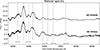 |
Fig. 13. Nebular spectra of SN 2020ue and SN 2020nlb, used for the analysis described in Sect. 4.4, with main line features identified. |
One method to infer the 56Ni mass involves reconstructing the luminosity evolution of the [Co III] 5893 Å line, which enables recovery of the line luminosity at specific epochs: 145 days for SN 2020ue and 147 days for SN 2020nlb after peak brightness. Faint [Co III] 5893 Å emission is also observed in the very late SN 2020ue spectra obtained with LRIS at 384 days post-peak brightness. The [Co III] line luminosity linearly correlates with the synthesised nickel mass, but only within a particular time range, for example during the nebular phase around ∼200 d from the explosion (Childress et al. 2015). Thus, we can estimate the 56Ni mass by correcting the measured luminosity at a given epoch for the corresponding 56Co decay lifetime shift, with the resulting uncertainties accounted for in the systematic error budget (σMNi = 0.2 M⊙). We followed Childress et al. (2015)’s prescriptions for measuring the [Co III] 5893 Å line flux. For all spectra, we refined the flux calibration using available photometry (see Sect. 2). Additionally, we applied host galaxy extinction correction for SN 2020nlb using the value reported by BAYESN in Sect. 3.1. Results are reported in Table 5. In summary, both SNe exhibit similar 56Ni masses: MNi = 0.50 ± 0.23 M⊙, consistent within uncertainties with estimates inferred in Sect. 3.4. Note that systematic uncertainties contribute significantly to the MNi uncertainty.
Measurements of the [Co III] 5893 Å nebular line flux and derived nickel mass for both SNe.
4.5. Analysis of the environment
Identifying interstellar medium (ISM) lines and diffuse interstellar bands (DIBs) in host galaxies from SN spectra allows for estimating host extinction along the line of sight (Phillips et al. 2013). Empirical relations can then provide extinction estimates from Na I equivalent width (EW) measurements (e.g. Munari & Zwitter 1997; Poznanski et al. 2012). Furthermore, the presence and potential variations of these lines could indicate the existence of a CSM around the SN progenitor star. To find out, we analysed high-resolution spectra obtained with Lick/APF at three epochs for SN 2020ue and two epochs for SN 2020nlb. Interestingly, neither the Lick/APF spectra nor the Asiago echelle spectrum of SN 2020nlb show Na ID lines (see Fig. B.8). We simulated Na ID lines using a Gaussian function with ∼20 km/s dispersion velocity and varying EW arbitrarily. We also considered a ±100 km/s velocity shift relative to each galaxy’s centre (grey regions in Fig. B.8). However, no match with narrow ISM/CSM features was found in the APF spectra of either SN, with an EW limit of EW < 0.015 Å. This sets a limit of E(B − V) < 0.02 mag (Poznanski et al. 2012).
5. Discussion
Photometric and spectroscopic analyses in Sects. 3 and 4 demonstrated that SN 2020nlb exhibits properties entirely consistent with normal SNe Ia. However, SN 2020ue is intriguing, displaying very blue colours at peak brightness comparable to or even bluer than transitional events. Additionally, SN 2020ue’s light curve evolution resembles the fast-declining SNe Ia sub-class, characterised by faster decline rates than normal SNe Ia. Its Δm15 value lies at the borderline between normal SNe Ia and the fast-declining sub-class. The rise time computed from the bolometric light curve, tr, 20ue = 14.48 ± 0.20 days, is similar to transitional and fast-declining events (Taubenberger et al. 2008).
High-resolution spectra of both events show no detectable Na I D absorption lines at the host’s redshift. Na I D EW measurements have been extensively used to estimate interstellar dust extinction based on empirical relations (e.g. Poznanski et al. 2012), although sodium is not a primary element of interstellar dust grains (Draine 2003). We therefore conclude that SN 2020nlb is intrinsically red due to SN ejecta temperature, rather than reddened by interstellar dust. However, as evident from its light curve characteristics, SN 2020nlb is a ‘normal’ SN at the edge to the transitional region in the luminosity-decay rate relation. Thus, SN 2020nlb may be the first SN of a small population of SNe Ia, which can be identified only through a detailed analysis of their local host galaxy environments. High-cadenced SN light curve coverage is also required. Furthermore, the distance estimate differences between SN 2020ue and SN 2020nlb align with their respective host galaxies’ distance moduli obtained using different distance methods, considering the extent of the Virgo cluster Δμ = 0.32 ± 0.06 mag (Mei et al. 2007). We emphasise that SBF- or FP-derived distances to the host galaxies of SN 2020ue and SN 2020nlb agree with those obtained via SNe Ia light curve fitting methods, but are characterised by larger uncertainties, see Table 2.
Our spectral analysis revealed that SN 2020ue and SN 2020nlb belong to the CN and BL sub-classes, respectively, in the Branch classification scheme defined by Branch et al. (2006) (see Fig. 10). This implies that both SNe share spectral properties with the bulk of normal SNe Ia, unlike transitional and fast-declining sub-types, characterised by larger Si II 5972 Å pEWs and classified within the CL sub-class by definition. This evidence suggests that spectroscopic diagnostics can clarify the true nature of SNe Ia explosions and provide crucial information about the underlying progenitor WD’s physical properties. Numerous studies have linked faint SNe Ia light curve properties to various WD progenitor properties (e.g. Hoeflich et al. 2017; Ashall et al. 2018). Within the SD progenitor models, one possible explanation is that a higher central density of the WD can result in more stable 58Ni production at the expense of 56Ni (Hoeflich et al. 2017; Ashall et al. 2018). A lower synthesised 56Ni amount leads to less ejecta heating and, consequently, faint peak luminosities, low ejecta temperatures, and enhanced low-ionisation features such as Ti II in SN Ia spectra. This contrasts with the large Si II 5972 Å pEWs observed in faint SNe Ia, given the higher excitation energy required for Si II 5972 Å compared to Si II 6355 Å. However, at lower temperatures, Si II is more abundant than the higher ionisation Si III line, which is more prominent in luminous SNe Ia spectra (e.g. Ashall et al. 2016). This indicates that high Si II 5972 Å intensity implies a low-ionisation level for the entire SN ejecta, aligning with the lower excitation temperature observed for transitional events compared to normal SNe Ia at similar epochs.
The detection of carbon in SN 2020ue and its non-detection in SN 2020nlb at very early epochs has significant implications for understanding their progenitor systems. Carbon features in SNe Ia spectra can provide crucial insights into the amount of unburned material, helping to differentiate between scenarios involving the progenitor WD’s nature and explosion dynamics. Unburned material serves as a vital indicator of the explosion mechanism, suggesting that the progenitor WD did not undergo complete thermonuclear burning before the explosion. Strong carbon absorption features are relatively rare (Parrent et al. 2011), typically observed during the pre-maximum phase of a small fraction of SNe Ia (Folatelli et al. 2012; Maguire et al. 2014). This could be attributed to low unburned material quantities or the blending of carbon lines with other spectral features such as Si II 6355 Å. Conversely, the absence of carbon lines could indicate a more complete burning process, implying that the progenitor WD might have been closer to the Chandrasekhar mass limit and experienced a more energetic explosion. Thomas et al. (2011) present evidence of unburned carbon in multiple SNe Ia, supporting the notion that the lack of such features in other events might be connected to distinct progenitor properties, such as sub-Chandrasekhar double-detonation models (Sim et al. 2010; Polin et al. 2019; Pakmor et al. 2022; Zenati et al. 2023) or explosion mechanisms (Heringer et al. 2019).
6. Conclusions and perspectives
In this work, we conducted a high-cadence photometric and spectroscopic follow-up campaign of two SNe Ia, SN 2020ue and SN 2020nlb, in two elliptical galaxies, NGC 4636 and NGC 4382, respectively. Our combined analysis of multi-filter SN evolution using light curve fitting codes such as SNOOPY, BAYESN, and GP-based methods, along with pseudo-bolometric light curves, derived 56Ni masses, and the entire spectral series, has revealed the following:
-
SN 2020nlb appears to be an intrinsically red yet otherwise normal SN Ia, with its colour arising from temperature rather than dust reddening. This provides evidence for intrinsic colour variation in normal SNe Ia, challenging standardisation methods such as the Tripp relation, and hinting at overlapping populations near the transitional regime.
-
The light curve and colour evolution of SN 2020ue, the rise-time to peak derived from the bolometric light curve (see Sect. 3.3), and the decay rate parametrised by sBV and Δm15 obtained from SNOOPY and BAYESN collectively demonstrate that this SN closely resembles the transitional SN sub-class, including SN 2007on and SN 2011iv, whose accuracy as distance indicators remains debated (Gall et al. 2018; Hoogendam et al. 2022).
-
The spectroscopic evolution shows that SN 2020ue is typical of the CN spectral class (Branch et al. 2006), whereas transitional and fast-decliner events display properties of the CL spectral class.
-
A spectral synthesis analysis of the UV plus optical peak brightness spectrum of SN 2020ue has been compared to a similar analysis of the UV plus optical spectrum at the same epoch of transitional SN 2011iv. The spectra show differences, particularly in the near-UV region due to line blanketing; therefore, we conclude that the peak spectrum of transitional SN 2011iv is richer in Fe-peak elements than SN 2020ue ejecta. This evidence can be attributed to mixing during the deflagration phase in SN 2011iv (Ashall et al. 2018).
-
The distance of these two SNe inferred from light curve fits and the luminosity-decay relation (Phillips 1993) aligns with their host distances estimated as a weighted average between the SBF and FP distance methods (Kourkchi et al. 2020) but display smaller uncertainties on the inferred distance moduli (see also Sects. 2.1 and 5).
-
The host extinction inferred from light curve fitting methods agrees with the absence of Na I D lines in SN 2020ue spectra but not SN 2020nlb, for which considerable colour excess (E(B − V)∼0.1 − 0.2 mag) has been estimated using different methods. This situation parallels the fast-decliner SN 2015bo (Hoogendam et al. 2022), suggesting caution when employing absorption-line empirical correlations to estimate host extinction in SNe.
Our results emphasise the importance of incorporating spectroscopic data to differentiate normal and peculiar events beyond traditional light curve fitting methods. Dedicated spectroscopic surveys are essential for constructing cosmological samples of SNe free from photometric biases, which is critical for their role as cosmological probes of the Universe’s expansion history and advancing our knowledge of the progenitor systems behind these phenomena.
Data availability
The spectroscopic data are available on WISeREP at the following links: SN 2020ue – https://www.wiserep.org/object/14941; SN 2020ue – https://www.wiserep.org/object/13914. The photometric dataset is available at the following link – https://github.com/lucagrb/SN2020nlb_SN2020ue. The analysis codes used in this work are available upon reasonable request to the corresponding author.
The tables of the photometry are available at the CDS via https://cdsarc.cds.unistra.fr/viz-bin/cat/J/A+A/706/A381
Acknowledgments
We thank G. Benetti for the realisation of trichomes in Figure 1, P. Butler and A. Kuehnel for their assistance with the reduction of the Lick/APF spectra, and C. Onken for his support in observing the environments of both SNe with WiFES at the 2.3-meter telescope of the Australian National University. This work is supported by a VILLUM FONDEN Young Investigator Grant (project number 25501, PI C. Gall), Villum Experiment grant (VIL69896) and by research grants (VIL16599, VIL54489) from VILLUM FONDEN. This material is based upon work supported by the National Science Foundation Graduate Research Fellowship Program under Grant Nos. 1842402 and 2236415. Any opinions, findings, conclusions, or recommendations expressed in this material are those of the authors and do not necessarily reflect the views of the National Science Foundation. L.I. acknowledges financial support from the INAF Data Grant Program “YES” (PI: Izzo) Multi-wavelength and multi messenger analysis of relativistic supernovae. S.M.W. was supported by the UK Science and Technology Facilities Council. Supernova and astrostatistics research at Cambridge University is supported by the European Union’s Horizon 2020 research and innovation programme under European Research Council Grant Agreement No. 101002652 (PI K. Mandel) and Marie Skłodowska-Curie Grant Agreement No. 873089. The UCSC team is supported in part by NASA grants 80NSSC23K0301 and 80NSSC24K1411; NSF grants AST–1815935 and AST–1720756; and a fellowship from the David and Lucile Packard Foundation to R.J.F. S.D. acknowledges support from UK Research and Innovation (UKRI) under the UK government’s Horizon Europe funding Guarantee EP/Z000475/1 and a Junior Research Fellowship at Lucy Cavendish College. D.O.J. acknowledges support from NSF grants AST–2407632 and AST–2429450, NASA grant 80NSSC24M0023, and HST/JWST grants HST-GO-17128.028, HST-GO-16269.012, and JWST-GO-05324.031, awarded by the Space Telescope Science Institute (STScI), which is operated by the Association of Universities for Research in Astronomy, Inc., for NASA, under contract NAS5–26555. C.D.K. gratefully acknowledges support from the NSF through AST–2432037, the HST Guest Observer Program through HST-SNAP-17070 and HST-GO-17706, and from JWST Archival Research through JWST-AR-6241 and JWST-AR-5441. G.N. is funded by NSF CAREER grant AST–2239364, supported in-part by funding from Charles Simonyi. GN also gratefully acknowledges NSF support from AST–2206195, OAC–2311355, AST–2432428, as well as AST–2421845 and funding from the Simons Foundation for the NSF-Simons SkAI Institute. G.N. is also supported by the DOE through the Department of Physics at the University of Illinois, Urbana-Champaign (# 13771275), and support from the HST Guest Observer Program through HST-GO-16764 and HST-GO-17128 (PI: R. Foley). A.R. acknowledges financial support from the GRAWITA Large Program Grant (PI P. D’Avanzo) and the PRIN-INAF 2022 “Shedding light on the nature of gap transients: from the observations to the models”. M.R.S. is supported by the STScI Postdoctoral Fellowship. S.J.S., S.S., and K.W.S. acknowledge funding from STFC Grants ST/Y001605/1, a Royal Society Research Professorship and the Hintze Charitable Foundation. The Young Supernova Experiment (YSE) and its research infrastructure is supported by the European Research Council under the European Union’s Horizon 2020 research and innovation programme (ERC Grant Agreement 101002652, PI K. Mandel), the Heising-Simons Foundation (2018-0913, PI R. Foley; 2018-0911, PI R. Margutti), NASA (NNG17PX03C, PI R. Foley), NSF (AST–1720756, AST–1815935, PI R. Foley; AST–1909796, AST–1944985, PI R. Margutti), the David & Lucille Packard Foundation (PI R. Foley), VILLUM FONDEN (project 16599, PI J. Hjorth), and the Center for AstroPhysical Surveys (CAPS) at the National Center for Supercomputing Applications (NCSA) and the University of Illinois Urbana-Champaign. Pan-STARRS is a project of the Institute for Astronomy of the University of Hawaii, and is supported by the NASA SSO Near Earth Observation Program under grants 80NSSC18K0971, NNX14AM74G, NNX12AR65G, NNX13AQ47G, NNX08AR22G, 80NSSC21K1572, and by the State of Hawaii. The Pan-STARRS1 Surveys (PS1) and the PS1 public science archive have been made possible through contributions by the Institute for Astronomy, the University of Hawaii, the Pan-STARRS Project Office, the Max-Planck Society and its participating institutes, the Max Planck Institute for Astronomy, Heidelberg and the Max Planck Institute for Extraterrestrial Physics, Garching, The Johns Hopkins University, Durham University, the University of Edinburgh, the Queen’s University Belfast, the Harvard-Smithsonian Center for Astrophysics, the Las Cumbres Observatory Global Telescope Network Incorporated, the National Central University of Taiwan, STScI, NASA under grant NNX08AR22G issued through the Planetary Science Division of the NASA Science Mission Directorate, NSF grant AST–1238877, the University of Maryland, Eotvos Lorand University (ELTE), the Los Alamos National Laboratory, and the Gordon and Betty Moore Foundation. Parts of this research are based on observations made with the Nordic Optical Telescope (programme 60-408, PI: Izzo; programme 61-022, PI Angus) owned in collaboration by the University of Turku and Aarhus University, and operated jointly by Aarhus University, the University of Turku and the University of Oslo, representing Denmark, Finland and Norway, the University of Iceland and Stockholm University at the Observatorio del Roque de los Muchachos, La Palma, Spain, of the Instituto de Astrofisica de Canarias. Data presented here were obtained in part with ALFOSC, which is provided by the Instituto de Astrofisica de Andalucia (IAA) under a joint agreement with the University of Copenhagen and NOT. Some of the data presented herein were obtained at the Infrared Telescope Facility, which is operated by the University of Hawaii under contract 80HQTR24DA010 with the National Aeronautics and Space Administration. Some of the data presented herein were obtained at Keck Observatory, which is a private 501(c)3 non-profit organisation operated as a scientific partnership among the California Institute of Technology, the University of California, and the National Aeronautics and Space Administration. The Observatory was made possible by the generous financial support of the W. M. Keck Foundation. The authors wish to recognize and acknowledge the very significant cultural role and reverence that the summit of Maunakea has always had within the indigenous Hawaiian community. We are most fortunate to have the opportunity to conduct observations from this mountain. A major upgrade of the Kast spectrograph on the Shane 3 m telescope at Lick Observatory was made possible through generous gifts from the Heising-Simons Foundation as well as William and Marina Kast. Research at Lick Observatory is partially supported by a generous gift from Google. Partly based on observations collected at the Copernico 1.82-m Telescope and the robotic Schmidt 67/92 telescope operated by INAF – Osservatorio Astronomico di Padova at Asiago, Italy, and the Galileo 1.22m telescope operated by University of Padova (Dept. of Physics and Astronomy, DFA). This work makes use of data from the Las Cumbres Observatory global telescope network. We acknowledge the use of public data from the Swift data archive. YSE-PZ was developed by the UC Santa Cruz Transients Team, supported in part by NASA grants NNG17PX03C, 80NSSC19K1386, and 80NSSC20K0953; NSF grants AST–1518052, AST–1815935, and AST–1911206; the Gordon & Betty Moore Foundation; the Heising-Simons Foundation; a fellowship from the David and Lucile Packard Foundation to R. J. Foley; a Gordon and Betty Moore Foundation postdoctoral fellowship and a NASA Einstein fellowship, as administered through the NASA Hubble Fellowship program and grant HST-HF2-51462.001, to D. O. Jones; and a National Science Foundation Graduate Research Fellowship, administered through grant No. DGE-1339067, to D. A. Coulter.
References
- Aleo, P. D., Malanchev, K., Sharief, S., et al. 2023, ApJS, 266, 9 [NASA ADS] [CrossRef] [Google Scholar]
- Arnett, W. D. 1982, ApJ, 253, 785 [Google Scholar]
- Ashall, C., Mazzali, P. A., Pian, E., & James, P. A. 2016, MNRAS, 463, 1891 [NASA ADS] [CrossRef] [Google Scholar]
- Ashall, C., Mazzali, P. A., Stritzinger, M. D., et al. 2018, MNRAS, 477, 153 [Google Scholar]
- Ashall, C., Lu, J., Shappee, B. J., et al. 2022, ApJ, 932, L2 [NASA ADS] [CrossRef] [Google Scholar]
- Astropy Collaboration (Price-Whelan, A. M., et al.) 2022, ApJ, 935, 167 [NASA ADS] [CrossRef] [Google Scholar]
- Bailey, S., Aldering, G., Antilogus, P., et al. 2009, A&A, 500, L17 [NASA ADS] [CrossRef] [EDP Sciences] [Google Scholar]
- Benetti, S., Cappellaro, E., Mazzali, P. A., et al. 2005, ApJ, 623, 1011 [NASA ADS] [CrossRef] [Google Scholar]
- Bertin, E. 2010, Astrophysics Source Code Library [record ascl:1010.068] [Google Scholar]
- Blondin, S., Matheson, T., Kirshner, R. P., et al. 2012, AJ, 143, 126 [NASA ADS] [CrossRef] [Google Scholar]
- Blondin, S., Dessart, L., Hillier, D. J., & Khokhlov, A. M. 2013, MNRAS, 429, 2127 [NASA ADS] [CrossRef] [Google Scholar]
- Bloom, J. S., Kasen, D., Shen, K. J., et al. 2012, ApJ, 744, L17 [NASA ADS] [CrossRef] [Google Scholar]
- Boone, K., Aldering, G., Antilogus, P., et al. 2021a, ApJ, 912, 70 [NASA ADS] [CrossRef] [Google Scholar]
- Boone, K., Aldering, G., Antilogus, P., et al. 2021b, ApJ, 912, 71 [NASA ADS] [CrossRef] [Google Scholar]
- Boos, S. J., Townsley, D. M., Shen, K. J., Caldwell, S., & Miles, B. J. 2021, ApJ, 919, 126 [NASA ADS] [CrossRef] [Google Scholar]
- Branch, D., & Wheeler, J. C. 2017, Supernova Explosions (Germany: Springer-Verlag GmbH) [Google Scholar]
- Branch, D., Doggett, J. B., Nomoto, K., & Thielemann, F. K. 1985, ApJ, 294, 619 [CrossRef] [Google Scholar]
- Branch, D., Garnavich, P., Matheson, T., et al. 2003, AJ, 126, 1489 [NASA ADS] [CrossRef] [Google Scholar]
- Branch, D., Dang, L. C., Hall, N., et al. 2006, PASP, 118, 560 [NASA ADS] [CrossRef] [Google Scholar]
- Brown, P. J., Breeveld, A. A., Holland, S., Kuin, P., & Pritchard, T. 2014, Ap&SS, 354, 89 [Google Scholar]
- Burns, C. R., Stritzinger, M., Phillips, M. M., et al. 2011, AJ, 141, 19 [Google Scholar]
- Burns, C. R., Stritzinger, M., Phillips, M. M., et al. 2014, ApJ, 789, 32 [Google Scholar]
- Burrow, A., Baron, E., Ashall, C., et al. 2020, ApJ, 901, 154 [NASA ADS] [CrossRef] [Google Scholar]
- Chambers, K. C., Magnier, E. A., Metcalfe, N., et al. 2016, arXiv e-prints [arXiv:1612.05560] [Google Scholar]
- Childress, M. J., Vogt, F. P. A., Nielsen, J., & Sharp, R. G. 2014, Ap&SS, 349, 617 [Google Scholar]
- Childress, M. J., Hillier, D. J., Seitenzahl, I., et al. 2015, MNRAS, 454, 3816 [NASA ADS] [CrossRef] [Google Scholar]
- Clocchiatti, A., & Wheeler, J. C. 1997, ApJ, 491, 375 [Google Scholar]
- Colgate, S. A., & McKee, C. 1969, ApJ, 157, 623 [NASA ADS] [CrossRef] [Google Scholar]
- Coulter, D. A., Jones, D. O., McGill, P., et al. 2022, https://doi.org/10.5281/zenodo.7278430 [Google Scholar]
- Coulter, D. A., Jones, D. O., McGill, P., et al. 2023, PASP, 135, 064501 [Google Scholar]
- Cushing, M. C., Vacca, W. D., & Rayner, J. T. 2004, PASP, 116, 362 [NASA ADS] [CrossRef] [Google Scholar]
- Dan, M., Guillochon, J., Brüggen, M., Ramirez-Ruiz, E., & Rosswog, S. 2015, MNRAS, 454, 4411 [Google Scholar]
- de Vaucouleurs, G. 1961, ApJS, 6, 213 [NASA ADS] [CrossRef] [Google Scholar]
- Desai, D. D., Kochanek, C. S., Shappee, B. J., et al. 2024, MNRAS, 530, 5016 [NASA ADS] [CrossRef] [Google Scholar]
- Dhawan, S., Leibundgut, B., Spyromilio, J., & Maguire, K. 2015, MNRAS, 448, 1345 [NASA ADS] [CrossRef] [Google Scholar]
- Dhawan, S., Bulla, M., Goobar, A., et al. 2018, MNRAS, 480, 1445 [NASA ADS] [CrossRef] [Google Scholar]
- Dimitriadis, G., Foley, R. J., Rest, A., et al. 2019, ApJ, 870, L1 [NASA ADS] [CrossRef] [Google Scholar]
- Dopita, M., Hart, J., McGregor, P., et al. 2007, Ap&SS, 310, 255 [Google Scholar]
- Dopita, M., Rhee, J., Farage, C., et al. 2010, Ap&SS, 327, 245 [Google Scholar]
- Draine, B. T. 2003, ARA&A, 41, 241 [NASA ADS] [CrossRef] [Google Scholar]
- Dutta, A., Singh, A., Anupama, G. C., Sahu, D. K., & Kumar, B. 2021, MNRAS, 503, 896 [Google Scholar]
- Elias, J. H., Matthews, K., Neugebauer, G., & Persson, S. E. 1985, ApJ, 296, 379 [NASA ADS] [CrossRef] [Google Scholar]
- Fausnaugh, M. M., Vallely, P. J., Tucker, M. A., et al. 2023, ApJ, 956, 108 [Google Scholar]
- Filippenko, A. V. 1982, PASP, 94, 715 [Google Scholar]
- Filippenko, A. V. 1997, ARA&A, 35, 309 [NASA ADS] [CrossRef] [Google Scholar]
- Filippenko, A. V., Richmond, M. W., Branch, D., et al. 1992a, AJ, 104, 1543 [NASA ADS] [CrossRef] [Google Scholar]
- Filippenko, A. V., Richmond, M. W., Matheson, T., et al. 1992b, ApJ, 384, L15 [CrossRef] [Google Scholar]
- Fink, M., Hillebrandt, W., & Röpke, F. K. 2007, A&A, 476, 1133 [NASA ADS] [CrossRef] [EDP Sciences] [Google Scholar]
- Fiore, A., Fraser, M., Kotak, R., et al. 2020, Transient Name Server AstroNote, 127, 1 [NASA ADS] [Google Scholar]
- Firth, R. E., Sullivan, M., Gal-Yam, A., et al. 2015, MNRAS, 446, 3895 [NASA ADS] [CrossRef] [Google Scholar]
- Fisher, R., & Jumper, K. 2015, ApJ, 805, 150 [NASA ADS] [CrossRef] [Google Scholar]
- Fisher, A., Branch, D., Nugent, P., & Baron, E. 1997, ApJ, 481, L89 [Google Scholar]
- Fitzpatrick, E. L. 1999, PASP, 111, 63 [Google Scholar]
- Flewelling, H. A., Magnier, E. A., Chambers, K. C., et al. 2020, ApJS, 251, 7 [NASA ADS] [CrossRef] [Google Scholar]
- Folatelli, G., Phillips, M. M., Burns, C. R., et al. 2010, AJ, 139, 120 [Google Scholar]
- Folatelli, G., Phillips, M. M., Morrell, N., et al. 2012, ApJ, 745, 74 [Google Scholar]
- Foley, R. J., & Kasen, D. 2011, ApJ, 729, 55 [Google Scholar]
- Foley, R. J., Kromer, M., Howie Marion, G., et al. 2012, ApJ, 753, L5 [Google Scholar]
- Förster, F., González-Gaitán, S., Folatelli, G., & Morrell, N. 2013, ApJ, 772, 19 [CrossRef] [Google Scholar]
- Gall, C., Stritzinger, M. D., Ashall, C., et al. 2018, A&A, 611, A58 [NASA ADS] [CrossRef] [EDP Sciences] [Google Scholar]
- Ganeshalingam, M., Li, W., & Filippenko, A. V. 2011, MNRAS, 416, 2607 [NASA ADS] [CrossRef] [Google Scholar]
- Gehrels, N., Chincarini, G., Giommi, P., et al. 2004, ApJ, 611, 1005 [Google Scholar]
- González-Gaitán, S., Perrett, K., Sullivan, M., et al. 2011, ApJ, 727, 107 [Google Scholar]
- González-Gaitán, S., Conley, A., Bianco, F. B., et al. 2012, ApJ, 745, 44 [Google Scholar]
- Graham, M. L., Kumar, S., Hosseinzadeh, G., et al. 2017, MNRAS, 472, 3437 [CrossRef] [Google Scholar]
- Graur, O. 2024, MNRAS, 530, 4950 [NASA ADS] [CrossRef] [Google Scholar]
- Guy, J., Astier, P., Nobili, S., Regnault, N., & Pain, R. 2005, A&A, 443, 781 [NASA ADS] [CrossRef] [EDP Sciences] [Google Scholar]
- Guy, J., Astier, P., Baumont, S., et al. 2007, A&A, 466, 11 [NASA ADS] [CrossRef] [EDP Sciences] [Google Scholar]
- Hachinger, S., Mazzali, P. A., & Benetti, S. 2006, MNRAS, 370, 299 [NASA ADS] [Google Scholar]
- Hachinger, S., Mazzali, P. A., Tanaka, M., Hillebrandt, W., & Benetti, S. 2008, MNRAS, 389, 1087 [NASA ADS] [CrossRef] [Google Scholar]
- Hamuy, M., Maza, J., Phillips, M. M., et al. 1993, AJ, 106, 2392 [NASA ADS] [CrossRef] [Google Scholar]
- Heringer, E., van Kerkwijk, M. H., Sim, S. A., Kerzendorf, W. E., & Graham, M. L. 2019, ApJ, 871, 250 [CrossRef] [Google Scholar]
- Hillebrandt, W., Kromer, M., Röpke, F. K., & Ruiter, A. J. 2013, Front. Phys., 8, 116 [Google Scholar]
- Hoeflich, P., Mueller, E., & Khokhlov, A. 1993, A&A, 268, 570 [Google Scholar]
- Hoeflich, P., Hsiao, E. Y., Ashall, C., et al. 2017, ApJ, 846, 58 [Google Scholar]
- Höflich, P., Gerardy, C. L., Fesen, R. A., & Sakai, S. 2002, ApJ, 568, 791 [NASA ADS] [CrossRef] [Google Scholar]
- Höflich, P., Krisciunas, K., Khokhlov, A. M., et al. 2010, ApJ, 710, 444 [Google Scholar]
- Höflich, P., Dragulin, P., Mitchell, J., et al. 2013, Front. Phys., 8, 144 [Google Scholar]
- Hoogendam, W. B., Ashall, C., Galbany, L., et al. 2022, ApJ, 928, 103 [NASA ADS] [CrossRef] [Google Scholar]
- Hoogendam, W. B., Shappee, B. J., Brown, P. J., et al. 2024, ApJ, 966, 139 [NASA ADS] [CrossRef] [Google Scholar]
- Hoogendam, W. B., Jones, D. O., Ashall, C., et al. 2025, Open J. Astrophys., 8, 120 [Google Scholar]
- Horne, K. 1986, PASP, 98, 609 [Google Scholar]
- Hosseinzadeh, G., Sand, D. J., Valenti, S., et al. 2017, ApJ, 845, L11 [NASA ADS] [CrossRef] [Google Scholar]
- Hsiao, E. Y., Conley, A., Howell, D. A., et al. 2007, ApJ, 663, 1187 [Google Scholar]
- Hsiao, E. Y., Marion, G. H., Phillips, M. M., et al. 2013, ApJ, 766, 72 [Google Scholar]
- Hsiao, E. Y., Burns, C. R., Contreras, C., et al. 2015, A&A, 578, A9 [NASA ADS] [CrossRef] [EDP Sciences] [Google Scholar]
- Iben, I., & Tutukov, A. V. 1984, ApJS, 54, 335 [NASA ADS] [CrossRef] [Google Scholar]
- Itagaki, K. 2020, Transient Name Server Discovery Report, 2020-111, 1 [Google Scholar]
- Iwamoto, K., Brachwitz, F., Nomoto, K., et al. 1999, ApJS, 125, 439 [NASA ADS] [CrossRef] [Google Scholar]
- Jack, D., Hauschildt, P. H., & Baron, E. 2012, A&A, 538, A132 [NASA ADS] [CrossRef] [EDP Sciences] [Google Scholar]
- Jones, D. O., Foley, R. J., Narayan, G., et al. 2021, ApJ, 908, 143 [NASA ADS] [CrossRef] [Google Scholar]
- Kasen, D. 2006, ApJ, 649, 939 [NASA ADS] [CrossRef] [Google Scholar]
- Kasen, D., & Woosley, S. E. 2007, ApJ, 656, 661 [NASA ADS] [CrossRef] [Google Scholar]
- Kasliwal, M. M., Ofek, E. O., Gal-Yam, A., et al. 2008, ApJ, 683, L29 [NASA ADS] [CrossRef] [Google Scholar]
- Kawabata, M. 2020, Transient Name Server Classification Report, 2020-114, 1 [Google Scholar]
- Kerzendorf, W. E., & Sim, S. A. 2014, MNRAS, 440, 387 [NASA ADS] [CrossRef] [Google Scholar]
- Kerzendorf, W., Nöbauer, U., Sim, S., et al. 2018, https://doi.org/10.5281/zenodo.1292315 [Google Scholar]
- Khatami, D. K., & Kasen, D. N. 2019, ApJ, 878, 56 [NASA ADS] [CrossRef] [Google Scholar]
- Khetan, N., Izzo, L., Branchesi, M., et al. 2021, A&A, 647, A72 [NASA ADS] [CrossRef] [EDP Sciences] [Google Scholar]
- Khokhlov, A. M. 1991, A&A, 245, 114 [NASA ADS] [Google Scholar]
- Kilpatrick, C. D., Foley, R. J., Drout, M. R., et al. 2018, MNRAS, 473, 4805 [NASA ADS] [CrossRef] [Google Scholar]
- Kostov, A., & Bonev, T. 2018, Bulg. Astron. J., 28, 3 [Google Scholar]
- Kourkchi, E., Tully, R. B., Eftekharzadeh, S., et al. 2020, ApJ, 902, 145 [NASA ADS] [CrossRef] [Google Scholar]
- Kromer, M., & Sim, S. A. 2009, MNRAS, 398, 1809 [Google Scholar]
- Kuchner, M. J., Kirshner, R. P., Pinto, P. A., & Leibundgut, B. 1994, ApJ, 426, L89 [NASA ADS] [CrossRef] [Google Scholar]
- Leibundgut, B., Kirshner, R. P., Phillips, M. M., et al. 1993, AJ, 105, 301 [NASA ADS] [CrossRef] [Google Scholar]
- Li, W., Leaman, J., Chornock, R., et al. 2011a, MNRAS, 412, 1441 [NASA ADS] [CrossRef] [Google Scholar]
- Li, W., Bloom, J. S., Podsiadlowski, P., et al. 2011b, Nature, 480, 348 [NASA ADS] [CrossRef] [Google Scholar]
- Lira, P. 1996, MS Thesis, Univ. Chile [Google Scholar]
- Liu, Z.-W., Röpke, F. K., & Han, Z. 2023, RAA, 23, 082001 [NASA ADS] [Google Scholar]
- Livio, M., & Mazzali, P. 2018, Phys. Rep., 736, 1 [Google Scholar]
- Lyman, J. D., Bersier, D., James, P. A., et al. 2016, MNRAS, 457, 328 [Google Scholar]
- Ma, X., Wang, X., Mo, J., et al. 2025, A&A, 698, A305 [NASA ADS] [CrossRef] [EDP Sciences] [Google Scholar]
- Maeda, K., Leloudas, G., Taubenberger, S., et al. 2011, MNRAS, 413, 3075 [Google Scholar]
- Magee, M. R., & Maguire, K. 2020, A&A, 642, A189 [NASA ADS] [CrossRef] [EDP Sciences] [Google Scholar]
- Magnier, E. A., Chambers, K. C., Flewelling, H. A., et al. 2020, ApJS, 251, 3 [NASA ADS] [CrossRef] [Google Scholar]
- Maguire, K. 2017, in Type Ia Supernovae, eds. A. W. Alsabti, & P. Murdin, 293 [Google Scholar]
- Maguire, K., Sullivan, M., Pan, Y. C., et al. 2014, MNRAS, 444, 3258 [NASA ADS] [CrossRef] [Google Scholar]
- Mandel, K. S., Thorp, S., Narayan, G., Friedman, A. S., & Avelino, A. 2022, MNRAS, 510, 3939 [NASA ADS] [CrossRef] [Google Scholar]
- Mazzali, P. A. 2001, MNRAS, 321, 341 [Google Scholar]
- Mazzali, P. A., Cappellaro, E., Danziger, I. J., Turatto, M., & Benetti, S. 1998, ApJ, 499, L49 [Google Scholar]
- Mazzali, P. A., Röpke, F. K., Benetti, S., & Hillebrandt, W. 2007, Science, 315, 825 [NASA ADS] [CrossRef] [Google Scholar]
- Mazzali, P. A., Sauer, D. N., Pastorello, A., Benetti, S., & Hillebrandt, W. 2008, MNRAS, 386, 1897 [Google Scholar]
- Mazzali, P. A., Sullivan, M., Hachinger, S., et al. 2014, MNRAS, 439, 1959 [NASA ADS] [CrossRef] [Google Scholar]
- Mazzali, P. A., Sullivan, M., Filippenko, A. V., et al. 2015, MNRAS, 450, 2631 [NASA ADS] [CrossRef] [Google Scholar]
- Mazzali, P. A., Ashall, C., Pian, E., et al. 2018, MNRAS, 476, 2905 [Google Scholar]
- McBrien, O. R., Smartt, S. J., Huber, M. E., et al. 2021, MNRAS, 500, 4213 [Google Scholar]
- McCully, C., Volgenau, N. H., Harbeck, D.-R., et al. 2018, SPIE Conf. Ser., 10707, 107070K [Google Scholar]
- Mei, S., Blakeslee, J. P., Côté, P., et al. 2007, ApJ, 655, 144 [Google Scholar]
- Miller, J. S., & Stone, R. P. S. 1993, Lick Obs. Tech. Rep. 66, LOTRM [Google Scholar]
- Miller, A. A., Magee, M. R., Polin, A., et al. 2020, ApJ, 898, 56 [NASA ADS] [CrossRef] [Google Scholar]
- Moriya, T. J., Mazzali, P. A., Ashall, C., & Pian, E. 2023, MNRAS, 522, 6035 [Google Scholar]
- Morrell, N., Phillips, M. M., Folatelli, G., et al. 2024, ApJ, 967, 20 [Google Scholar]
- Munari, U., & Zwitter, T. 1997, A&A, 318, 269 [NASA ADS] [Google Scholar]
- Murakami, Y. S., Riess, A. G., Stahl, B. E., et al. 2023, JCAP, 2023, 046 [CrossRef] [Google Scholar]
- Nadyozhin, D. K. 1994, ApJS, 92, 527 [Google Scholar]
- Ni, Y. Q., Moon, D.-S., Drout, M. R., et al. 2022, Nat. Astron., 6, 568 [Google Scholar]
- Ni, Y. Q., Moon, D.-S., Drout, M. R., et al. 2023a, ApJ, 946, 7 [Google Scholar]
- Ni, Y. Q., Moon, D.-S., Drout, M. R., et al. 2023b, ApJ, 959, 132 [Google Scholar]
- Ni, Y. Q., Moon, D.-S., Drout, M. R., et al. 2025, ApJ, 983, 3 [Google Scholar]
- Nomoto, K., Thielemann, F. K., & Yokoi, K. 1984, ApJ, 286, 644 [Google Scholar]
- Nugent, P., Phillips, M., Baron, E., Branch, D., & Hauschildt, P. 1995, ApJ, 455, L147 [NASA ADS] [CrossRef] [Google Scholar]
- Nugent, P. E., Sullivan, M., Cenko, S. B., et al. 2011, Nature, 480, 344 [NASA ADS] [CrossRef] [Google Scholar]
- Oke, J. B., Cohen, J. G., Carr, M., et al. 1995, PASP, 107, 375 [Google Scholar]
- Pakmor, R., Hachinger, S., Röpke, F. K., & Hillebrandt, W. 2011, A&A, 528, A117 [NASA ADS] [CrossRef] [EDP Sciences] [Google Scholar]
- Pakmor, R., Callan, F. P., Collins, C. E., et al. 2022, MNRAS, 517, 5260 [NASA ADS] [CrossRef] [Google Scholar]
- Pan, Y.-C., Foley, R. J., Kromer, M., et al. 2015, MNRAS, 452, 4307 [CrossRef] [Google Scholar]
- Pan, Y. C., Foley, R. J., Filippenko, A. V., & Kuin, N. P. M. 2018, MNRAS, 479, 517 [Google Scholar]
- Pankey, T. 1962, Ph.D. Thesis, Howard University, Washington DC [Google Scholar]
- Papadogiannakis, S. 2019, Ph.D. Thesis, Stockholm University [Google Scholar]
- Parrent, J. T., Thomas, R. C., Fesen, R. A., et al. 2011, ApJ, 732, 30 [Google Scholar]
- Pedregosa, F., Varoquaux, G., Gramfort, A., et al. 2011, J. Mach. Learn. Res., 12, 2825 [Google Scholar]
- Perets, H. B., Zenati, Y., Toonen, S., & Bobrick, A. 2019, arXiv e-prints [arXiv:1910.07532] [Google Scholar]
- Phillips, M. M. 1993, ApJ, 413, L105 [Google Scholar]
- Phillips, M. M. 2012, PASA, 29, 434 [NASA ADS] [CrossRef] [Google Scholar]
- Phillips, M. M., Wells, L. A., Suntzeff, N. B., et al. 1992, AJ, 103, 1632 [NASA ADS] [CrossRef] [Google Scholar]
- Phillips, M. M., Lira, P., Suntzeff, N. B., et al. 1999, AJ, 118, 1766 [Google Scholar]
- Phillips, M. M., Simon, J. D., Morrell, N., et al. 2013, ApJ, 779, 38 [NASA ADS] [CrossRef] [Google Scholar]
- Phillips, M. M., Ashall, C., Burns, C. R., et al. 2022, ApJ, 938, 47 [NASA ADS] [CrossRef] [Google Scholar]
- Pinto, P. A., & Eastman, R. G. 2000, ApJ, 530, 744 [Google Scholar]
- Piro, A. L., & Nakar, E. 2014, ApJ, 784, 85 [NASA ADS] [CrossRef] [Google Scholar]
- Polin, A., Nugent, P., & Kasen, D. 2019, ApJ, 873, 84 [Google Scholar]
- Poznanski, D., Prochaska, J. X., & Bloom, J. S. 2012, MNRAS, 426, 1465 [Google Scholar]
- Pskovskii, I. P. 1977, Sov. Astron., 21, 675 [NASA ADS] [Google Scholar]
- Rayner, J. T., Toomey, D. W., Onaka, P. M., et al. 2003, PASP, 115, 362 [NASA ADS] [CrossRef] [Google Scholar]
- Rest, A., Stubbs, C., Becker, A. C., et al. 2005, ApJ, 634, 1103 [NASA ADS] [CrossRef] [Google Scholar]
- Riess, A. G., Filippenko, A. V., Li, W., et al. 1999, AJ, 118, 2675 [NASA ADS] [CrossRef] [Google Scholar]
- Riess, A. G., Macri, L. M., Hoffmann, S. L., et al. 2016, ApJ, 826, 56 [Google Scholar]
- Ruiter, A. J., & Seitenzahl, I. R. 2025, A&ARv, 33, 1 [Google Scholar]
- Sand, D. 2014, in The Third Hot-wiring the Transient Universe Workshop, eds. P. R. Wozniak, M. J. Graham, A. A. Mahabal, & R. Seaman, 187 [Google Scholar]
- Sand, D. J., Sarbadhicary, S. K., Pellegrino, C., et al. 2021, ApJ, 922, 21 [NASA ADS] [CrossRef] [Google Scholar]
- Sauer, D. N., Mazzali, P. A., Blondin, S., et al. 2008, MNRAS, 391, 1605 [NASA ADS] [CrossRef] [Google Scholar]
- Schechter, P. L., Mateo, M., & Saha, A. 1993, PASP, 105, 1342 [Google Scholar]
- Schuberth, Y., Richtler, T., Dirsch, B., et al. 2006, A&A, 459, 391 [NASA ADS] [CrossRef] [EDP Sciences] [Google Scholar]
- Scolnic, D., Casertano, S., Riess, A., et al. 2015, ApJ, 815, 117 [Google Scholar]
- Seitenzahl, I. R., & Townsley, D. M. 2017, in Handbook of Supernovae, eds. A. W. Alsabti, & P. Murdin, 1955 [Google Scholar]
- Shen, K. J., Blondin, S., Kasen, D., et al. 2021, ApJ, 909, L18 [NASA ADS] [CrossRef] [Google Scholar]
- Shigeyama, T., Nomoto, K., Yamaoka, H., & Thielemann, F.-K. 1992, ApJ, 386, L13 [Google Scholar]
- Siebert, M. R., Foley, R. J., Jones, D. O., et al. 2019, MNRAS, 486, 5785 [CrossRef] [Google Scholar]
- Silverman, J. M., & Filippenko, A. V. 2012, MNRAS, 425, 1917 [NASA ADS] [CrossRef] [Google Scholar]
- Sim, S. A., Röpke, F. K., Hillebrandt, W., et al. 2010, ApJ, 714, L52 [Google Scholar]
- Smith, K. W., Smartt, S. J., Young, D. R., et al. 2020, PASP, 132, 085002 [Google Scholar]
- Stahl, B. E., Zheng, W., de Jaeger, T., et al. 2020, MNRAS, 492, 4325 [NASA ADS] [CrossRef] [Google Scholar]
- Stehle, M., Mazzali, P. A., Benetti, S., & Hillebrandt, W. 2005, MNRAS, 360, 1231 [NASA ADS] [CrossRef] [Google Scholar]
- Stritzinger, M., Mazzali, P. A., Sollerman, J., & Benetti, S. 2006, A&A, 460, 793 [NASA ADS] [CrossRef] [EDP Sciences] [Google Scholar]
- Stritzinger, M., Burns, C. R., Phillips, M. M., et al. 2010, AJ, 140, 2036 [Google Scholar]
- Swift, J. J., Andersen, K., Arculli, T., et al. 2022, PASP, 134, 035005 [Google Scholar]
- Tanaka, M., Mazzali, P. A., Stanishev, V., et al. 2011, MNRAS, 410, 1725 [Google Scholar]
- Taubenberger, S. 2017, in Handbook of Supernovae, eds. A. W. Alsabti, & P. Murdin, 317 [Google Scholar]
- Taubenberger, S., Hachinger, S., Pignata, G., et al. 2008, MNRAS, 385, 75 [NASA ADS] [CrossRef] [Google Scholar]
- Temi, P., Brighenti, F., & Mathews, W. G. 2007, ApJ, 666, 222 [Google Scholar]
- Thomas, R. C., Aldering, G., Antilogus, P., et al. 2007, ApJ, 654, L53 [NASA ADS] [CrossRef] [Google Scholar]
- Thomas, R. C., Aldering, G., Antilogus, P., et al. 2011, ApJ, 743, 27 [Google Scholar]
- Tonry, J. L., Denneau, L., Heinze, A. N., et al. 2018, PASP, 130, 064505 [Google Scholar]
- Townsend, A., Smith, K. W., Srivastav, S., et al. 2020, Transient Name Server AstroNote, 126, 1 [NASA ADS] [Google Scholar]
- Trentham, N., & Hodgkin, S. 2002, MNRAS, 333, 423 [NASA ADS] [CrossRef] [Google Scholar]
- Truran, J. W., Arnett, W. D., & Cameron, A. G. W. 1967, Can. J. Phys., 45, 2315 [NASA ADS] [CrossRef] [Google Scholar]
- Tucker, M. A., Shappee, B. J., Kochanek, C. S., et al. 2022, MNRAS, 517, 4119 [Google Scholar]
- Tully, R. B., Courtois, H. M., & Sorce, J. G. 2016, AJ, 152, 50 [Google Scholar]
- Valenti, S., Benetti, S., Cappellaro, E., et al. 2008, MNRAS, 383, 1485 [Google Scholar]
- Vogt, S. S., Radovan, M., Kibrick, R., et al. 2014, PASP, 126, 359 [NASA ADS] [CrossRef] [Google Scholar]
- Wang, X., Filippenko, A. V., Ganeshalingam, M., et al. 2009, ApJ, 699, L139 [NASA ADS] [CrossRef] [Google Scholar]
- Wang, X., Wang, L., Filippenko, A. V., Zhang, T., & Zhao, X. 2013, Science, 340, 170 [NASA ADS] [CrossRef] [Google Scholar]
- Wang, X., Chen, J., Wang, L., et al. 2019, ApJ, 882, 120 [NASA ADS] [CrossRef] [Google Scholar]
- Wang, Q., Rest, A., Zenati, Y., et al. 2021, ApJ, 923, 167 [Google Scholar]
- Wang, Q., Rest, A., Dimitriadis, G., et al. 2024, ApJ, 962, 17 [Google Scholar]
- Ward, S. M., Thorp, S., Mandel, K. S., et al. 2023, ApJ, 956, 111 [NASA ADS] [CrossRef] [Google Scholar]
- Whelan, J., & Iben, I. 1973, ApJ, 186, 1007 [CrossRef] [Google Scholar]
- Williams, S. C., Kotak, R., Lundqvist, P., et al. 2024, A&A, 685, A135 [NASA ADS] [CrossRef] [EDP Sciences] [Google Scholar]
- Woosley, S. E., & Weaver, T. A. 1986, ARA&A, 24, 205 [NASA ADS] [CrossRef] [Google Scholar]
- Woosley, S. E., Kasen, D., Blinnikov, S., & Sorokina, E. 2007, ApJ, 662, 487 [NASA ADS] [CrossRef] [Google Scholar]
- Woosley, S. E., Sukhbold, T., & Kasen, D. N. 2021, ApJ, 913, 145 [NASA ADS] [CrossRef] [Google Scholar]
- Wyatt, S. D., Sand, D. J., Hsiao, E. Y., et al. 2021, ApJ, 914, 57 [Google Scholar]
- Yamaoka, H., Nomoto, K., Shigeyama, T., & Thielemann, F.-K. 1992, ApJ, 393, L55 [Google Scholar]
- Zenati, Y., Perets, H. B., Dessart, L., et al. 2023, ApJ, 944, 22 [NASA ADS] [CrossRef] [Google Scholar]
- Zeng, X., Wang, X., Esamdin, A., et al. 2021, ApJ, 909, 176 [NASA ADS] [CrossRef] [Google Scholar]
- Zhao, X., Maeda, K., Wang, X., & Sai, H. 2021, MNRAS, 503, 4667 [NASA ADS] [CrossRef] [Google Scholar]
ECSNOOPY is a package for SN photometry through PSF fitting and template subtraction, developed by E. Cappellaro, 2014. See also https://sngroup.oapd.inaf.it/ecsnoopy.html
Appendix A: Data reduction
A.1. Photometry
In addition to Pan-STARRS data, we also obtained photometric coverage for SN 2020ue and SN 2020nlb with other facilities. Regarding SN 2020ue, a photometric coverage of the peak brightness until late epochs was obtained with the Alhambra Faint Object Spectrograph and Camera (ALFOSC) mounted at the Nordic Optical Telescope (NOT) located in La Palma, Canary Islands, Spain, using uBVgriz filters, and both SNe 2020ue and 2020nlb were observed with the Asiago Faint Object Spectrograph and Camera (AFOSC) mounted at the 1.82m telescope and with the robotic Schmidt 67/92 telescope (both located at Cima Ekar, Asiago, Italy), using the same filter setup. The calibrated photometry was derived with the ECSNOOPY pipeline2, using the PSF-fitting technique on the science images. The instrumental magnitudes were then calibrated to the Sloan AB system, using Sloan stars in the field of the host galaxy. Given the smoothness of the underlying stellar background, PSF photometry has been performed by fitting the underlying background up to three times the FWHM of the target, and finally checking the smoothness of the residual image, after subtracting the PSF fit of the target. Error estimates for the SN magnitudes are obtained through artificial star experiments in which fake stars with similar magnitudes as the SN are placed in the fit residual image in a position close to, but not coincident with, the SN location. The simulated images were processed using the same procedure, and the standard deviation of the measured magnitudes of the fake stars was taken as an estimate of the instrumental magnitude error. In practical terms, this error mainly reflects uncertainty in the background subtraction.
Both SNe were also observed by the Neil Gehrels Swift observatory (Gehrels et al. 2004). We reduced Swift/UVOT data using UVOTSOURCE using the HEASOFT v6.26 software package following the standard procedures as described in Brown et al. (2014). We used a 3″ aperture size with a 30″ region to estimate the background contribution around each source. The final Swift/UVOT light curve for both sources is shown in Fig. 2.
We observed SN 2020ue, and SN 2020nlb in uBVgri bands with the Direct 4K×4K imager on the Swope 1 m telescope at Las Campanas Observatory, Chile. Following procedures described in Kilpatrick et al. (2018), all imaging data were reduced using PHOTPIPE (Rest et al. 2005), including corrections for bias, flat-fielding, amplifier crosstalk corrections, astrometric distortion corrections and regridding of each image using SWARP (Bertin 2010), photometry using DOPHOT (Schechter et al. 1993), and photometric calibration using the Pan-STARRS DR2 catalogue (Flewelling et al. 2020) transformed to the Swope in-band natural magnitudes using Supercal (Scolnic et al. 2015). Final Swope photometry was obtained at the site of both sources using forced DOPHOT photometry in the final images.
We observed SN 2020nlb in griz bands with the Thacher 0.7 m telescope at the Thacher School Observatory in Ojai, CA (Swift et al. 2022). Following the same procedures described above for Swope, we obtained the final photometry of the SN using PHOTPIPE.
We observed SN 2020ue and SN 2020nlb in uBVgri bands with the Sinistro imagers on the Las Cumbres Observatory (LCO) 1 m telescopes. Taking the BANZAI processed images from the LCO pipeline (McCully et al. 2018), we corrected the reduced images for geometric distortion using SWARP and performed photometry and flux calibration using the same PHOTPIPE procedures described above. The final photometry for both sources is forced DOPHOT photometry in the final reduced frames.
Observations of SN 2020nlb were conducted using the 0.5-meter telescope at the Osservatorio Astronomico "Salvatore Di Giacomo" (OASDG) in Agerola, Italy3. BVR images were acquired during the initial 60 days of SN emission, with data reduction and calibration performed via a dedicated pipeline based on the Astropy package (Astropy Collaboration 2022). Magnitudes were calculated using an astropy-based aperture photometry routine on single-epoch stacked images and converted to BVR magnitudes using transformation formulas from (Kostov & Bonev 2018). The resulting OASDG light curve is depicted in Fig. B.6 alongside the complete dataset.
A.2. Spectroscopy
Five spectroscopic epochs of SN 2020nlb were observed using grism #4 on the NOT with ALFOSC, covering the 3,800-9,400 Å wavelength range and a resolving power of R = 360. Data reduction was performed with PYNOT4, a Python-based GUI tailored for ALFOSC. The software enables standard calibrations, background subtraction using Chebyshev polynomial approximation, and flux calibration using a standard star.
We observed SN 2020ue and SN 2020nlb with the FLOYDS spectrographs (Sand 2014) on the Faulkes 2 m North and South telescopes at Haleakala, Hawaii and Siding Spring Observatory, Australia, respectively. All FLOYDS data were processed using the LCO FLOYDS pipeline as described in McCully et al. (2018).
Twenty spectroscopic epochs of SN 2020ue were obtained in Asiago, Italy, using both the Copernico 1.82m telescope, equipped with AFOSC or with an Echelle high-resolution spectrograph, and with the Galileo 1.22m telescope equipped with a Boller & Chivens spectrograph. The slit was set at the parallactic angle. The spectra were reduced using standard IRAF tasks for the data reduction. After bias and flat-field correction, the SN spectrum was extracted and calibrated in wavelength with reference to standard arc lamp spectra. For the flux calibration, nightly sensitivity functions were derived from observations of spectrophotometric standard stars such as Feige 34, Feige 56 and HR 3154, and also used to derive the corrections for the telluric absorption bands. The flux calibration of each spectrum was verified against coeval broadband photometry.
We obtained additional optical follow-up spectroscopy with the Low-Resolution Imaging Spectrograph (LRIS; Oke et al. 1995) on the 10-m Keck I telescope and the Kast dual-beam spectrograph (Miller & Stone 1993) on the Lick Shane 3-m telescope. We obtained two epochs of SN 2020ue, and one epoch of SN 2020nlb with LRIS, and we obtained five epochs of SN 2020ue, and SN 2020nlb, respectively, with Kast. Observations with Kast were taken with the slit at the parallactic angle (Filippenko 1982) to reduce flux losses associated with aligning the slit at non-parallactic angles. Observations with LRIS were aligned to the nucleus of the host galaxy since LRIS is equipped with an atmospheric dispersion corrector. We reduced the Kast and LRIS spectral data in a standard manner using our custom data-reduction UCSC SPECTRAL PIPELINE5 (Siebert et al. 2019). The 2D spectra were bias-corrected, flat-field corrected, adjusted for varying gains across different chips and amplifiers, and trimmed. We combined multiple frames using a sigma-clipping cosmic algorithm to remove cosmic rays. 1D spectra were then extracted using the optimal algorithm (Horne 1986). The spectra were wavelength-calibrated using internal arc lamps spectra. The wavelength solution was refined by applying linear shifts determined by cross-correlating the observed night-sky lines to a master night-sky spectrum, and a heliocentric correction was applied. Flux calibration was performed relative to standard stars using the same setup and, where possible, a similar airmass to that of the science exposures with ‘blue’ (hot subdwarfs; i.e. sdO) and ’red’ (low-metallicity G/F) standard stars corrected for atmospheric extinction. To remove atmospheric absorption features in the spectra, a telluric correction was determined by fitting the continuum of the flux-calibrated red standard stars to create a normalised spectrum only including telluric features. The relative strength of the absorption was determined by calculating the relative airmass between the standard star and the science image. The telluric bands of the red standard star were cross-correlated with the supernova spectrum at the B band and the A band to calculate small wavelength shifts, which were averaged and applied. We then combined the red and blue sides by rescaling one spectrum to match the flux of the other in the overlap region between the blue and red sides.
We acquired three epochs of SN 2020ue and two epochs of SN 2020nlb using the Automated Planet Finder (APF; Vogt et al. 2014), a robotic 2.4 m telescope located at Lick Observatory. The APF is equipped with the Levy Spectrograph, a high-resolution (R ≃ 100,000) echelle spectrograph, with a wavelength coverage of 3740-9700 Å. These data were reduced using a custom raw reduction package developed for Iodine-based precision velocity spectrometers by the APF team. The reduction package performed standard flat fielding, scattered light subtraction, order tracing, and cosmic ray removal. The spectra were wavelength calibrated against the NIST Fourier Transform Spectrometer spectral atlas of the APF Iodine cell, with a resolution of 1,000,000 and a S/N ∼1,000. Telluric lines were identified by comparing the spectrum of a rapidly rotating B star to a synthetic telluric atlas. With the exception of telluric lines, the spectrum of the rapidly rotating B star is nearly featureless. Pixels with telluric lines were given zero weight for the wavelength and velocity determination. The final spectra are presented in vacuum wavelengths.
SN 2020ue was observed with the SpeX medium-resolution spectrograph (Rayner et al. 2003) mounted on the NASA Infrared Telescope Facility (IRTF), located on Mauna Kea (Hawaii, USA). We present two NIR spectra obtained on Days −5 and +56 (Program ID 2019B087, PI M. Shahbandeh). Data were reduced using the Spextool package with standard procedures and telluric corrections performed with an A0 star (Cushing et al. 2004)
Both SN 2020ue and SN 2020nlb were observed using the Wide Field Spectrograph (WiFeS) on the 2.3 m telescope at Siding Spring Observatory (Dopita et al. 2007, 2010) on 6 March 2021 and 12 May 2021, respectively. Each SN was observed using an RT-560 beam splitter and a B3000 and R3000 diffraction gratings that cover the 3200 − 5900 Å and 5300 − 9800 Å wavelength ranges. All observations have a 1x1 arcsec spaxel. The average seeing on each night was 1.7 arcsecs. Calibration data and standard star spectra were taken on each night, while each WiFeS observation was reduced using PyWiFeS (Childress et al. 2014), resulting in a 3D cube file having bad pixels and cosmic rays removed.
Finally, a single spectrum of SN 2020ue was obtained with the UltraViolet and Optical Telescope (UVOT) on board the Neil Gehrels Swift spacecraft (Gehrels et al. 2004). The spectrum was obtained on 19 January 2020 (MJD 58867.47), using the slitless grism mode. We used the same recipes for data reduction and spectra extraction that are reported in Pan et al. (2018).
Appendix B: Additional figures and tables
This section includes additional Figures and Tables that support the results presented in the main text.
Table B.1 shows the diary of the spectroscopic observations presented in this work.
Table B.2 shows the measurements of the pEWs measured in SN 2020ue and SN 2020nlb using the SPEXTRACTOR code.
Figure B.1 shows the best-fit results and parameters posterior distribution obtained applying BAYESN to the multi-filter light curves of SN 2020ue and SN 2020nlb.
Figures B.2, B.3 refer to the analysis of the bolometric luminosity of SN 2020ue and SN 2020nlb discussed in Secs. 3.2-3.4.
Figure B.4 shows the best-fit results of the OASDG B and V light curves of SN 2020ue and SN 2020nlb obtained using the GP process described in Sec. 3.1, with the results reported in Table 1. Similarly, Figures B.6 shows the SNOOPY best-fit results of the multi-filter light curves of SN 2020ue and SN 2020nlb obtained with LCO, Thatcher and OASDG, with results reported in Table B.3.
Figure B.5 shows the best-fit model obtained for the peak spectrum of SN 2020ue using the SPEXTRACTOR code, with the identification of the main absorption features highlighted with grey regions.
Figure B.7 shows the Branch plot distribution of the pEW(Si II 5972) against the Δm15 value, and the ratio of pEW of both Si II lines, R(Si II) versus Δm15 value, for a set of SNe Ia for which the pEW has been measured using the same methodology adapted in this work, for example with SPEXTRACTOR (Burrow et al. 2020).
Figure B.8 shows the high-resolution spectra of SN 2020ue and SN 2020nlb obtained with the Asiago/Echelle instrument and the Lick/APF instrument in the rest-frame region around the Na I D line, showing absence of this feature in both SN spectra.
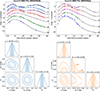 |
Fig. B.1. (Upper panels): Fit of the PS1 light curve of SN 2020nlb (left) and SN 2020ue (right). (Lower panels): Results from the MC analysis with BAYESN for the PS1 light curves of SN 2020nlb (left) and SN 2020ue (right). |
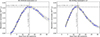 |
Fig. B.2. Bolometric light curves of SN 2020nlb (left panel) and SN 2020ue (right panel). The black curves represent the GP model employed to estimate the peak luminosity and epoch of each light curve. The determined epochs for the SN explosions correspond to those obtained using the photospheric velocity method proposed by Piro & Nakar (2014). |
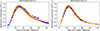 |
Fig. B.3. Fit of the SN 2020nlb (left panel) and SN 2020ue (right panel) bolometric light curves. The orange curves correspond to 200 samples from the posterior distributions of the best-fit results shown in Table 3. |
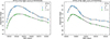 |
Fig. B.4. Light curve evolution of SN 2020nlb (left panel) and SN 2020ue (right panel) obtained using the GP regressor method. |
Log of spectroscopic observations.
pEW values (in milliångström) obtained for selected absorption lines using SPEXTRACTOR for the SN 2020ue and SN 2020nlb spectra.
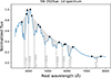 |
Fig. B.5. Measurements of the pEWs for SN 2020ue at −1 day using Spextractor. Shaded regions correspond to the area used to estimate the pEWs, with black circles marking the boundaries of each absorption feature. Black circles mark the position of the lower- and upper-boundary wavelength regions identified by the GP algorithm for each absorption line (Papadogiannakis 2019). |
Results of light curve fits made with SNOOPY using LCO data for SN 2020ue and OASDG data for SN 2020nlb.
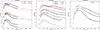 |
Fig. B.6. Fit obtained with SNOOPY (black curves) using LCO data (uBVgri) for SN 2020ue (left panel), and using Thacher (gri) and UVOT data for SN 2020nlb (middle panel), and OASDG data (BVR, right panel). The plot shows the results obtained using the max-model light curve model function and the sBV stretch-colour parameter. |
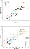 |
Fig. B.7. Same as Fig. 10, but with the distribution of the Δm15 parameter against the pEW of the Si II 5972 Å line (upper panel), and against the Si II ratio R(Si) (lower panel). Data shown in red, blue, green, and orange symbols are taken from Burrow et al. (2020) and respectively colour-coded according to the Branch spectroscopic sub-classes – SS, BL, CL, and CN. SN 2020ue and SN 2020nlb are highlighted as black and red stars, respectively. |
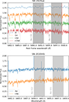 |
Fig. B.8. (Top): Asiago/Echelle spectrum (−8 d, blue curve) and Lick/APF spectra of SN 2020ue. (Bottom): Lick/APF spectra of SN 2020nlb. The spectra were obtained around the peak brightness of both supernovae. The grey regions mark the positions of the expected Na ID lines at the redshift of each supernova, accounting for a shift of ±100 km/s due to possible rotation velocity at each supernova position. |
All Tables
Physical properties from best-fit analysis of bolometric light curves of SN 2020nlb and SN 2020ue using using the analytical model.
Physical properties and element abundances obtained from the TARDIS simulation of day −5 spectra of SN 2020ue and day −6 of SN 2011iv.
Measurements of the [Co III] 5893 Å nebular line flux and derived nickel mass for both SNe.
pEW values (in milliångström) obtained for selected absorption lines using SPEXTRACTOR for the SN 2020ue and SN 2020nlb spectra.
Results of light curve fits made with SNOOPY using LCO data for SN 2020ue and OASDG data for SN 2020nlb.
All Figures
|
Fig. 1. Trichromy image from BVr single-filter observations with the Asiago Schmidt telescope a few days after the discoveries of SN 2020ue (left panel) and SN 2020nlb (right panel). The positions of these SN in their respective host galaxies are marked with white indicators. Courtesy of Giovanni Benetti (DFA, University of Padova). |
| In the text | |
|
Fig. 2. Light curve evolution of SN 2020ue (left panel) and SN 2020nlb (right panel). Symbols denote data from different facilities (diamonds: Swift-UVOT; triangles: Copernico-AFOSC, NOT-ALFOSC (for SN 2020ue), and Pan-STARRS (for SN 2020nlb); squares: Swope and Thacher; circles: LCO; pluses: OASDG), with colours indicating filters. Both light curves have not been corrected for Galactic reddening. |
| In the text | |
|
Fig. 3. Optical spectral series of SN 2020ue. Spectra were obtained with the Copernico 1.82m and Galileo 1.22m telescopes in Asiago, and the FLOYDS telescopes during the first 50 days of the SN evolution (left panel), and up to 390 days from B-band maximum (right panel). |
| In the text | |
|
Fig. 4. Optical spectral series of SN 2020nlb. Spectra were obtained with NOT, FLOYDS, and KAST. |
| In the text | |
|
Fig. 5. SNOOPY fits (black curves) to Swift-UVOT and Pan-STARRS gri data of SN 2020ue (left panel) and SN 2020nlb (right panel). The fits were obtained with the max-model light curve model function and the sBV stretch-colour parameter. |
| In the text | |
|
Fig. 6. Pan-STARRS g- and r- band light curves of SN 2020nlb (upper panel) and Copernico 1.82m B- and V-band SN 2020ue (lower panel), computed using the procedure outlined in Sect. 3.2. The dashed lines represent the best-fit obtained with a power-law model for the early light curve evolution (González-Gaitán et al. 2012). The most stringent ATLAS upper limit is indicated by an orange triangle, while an additional upper limit reported by Sand et al. (2021) 1.3 days later is marked by a red symbol at the time of the ATLAS observation. For SN 2020ue, the best-fit model extrapolation for the r band is consistent with these flux upper limits. |
| In the text | |
|
Fig. 7. Distribution of 56Ni masses for SN 2020nlb and SN 2020ue as a function of Δm15 determined using both the Khatami & Kasen (2019) method (blue data) and the Arnett (1982) analytical model (green data). For comparison, we include the Arnett model results (orange data) for the SNe Ia sample from Dhawan et al. (2018). The locations of the transitional and fast-declining events SN 2007on (Gall et al. 2018) and SN 2007ax (Kasliwal et al. 2008) are highlighted. |
| In the text | |
|
Fig. 8. Temporal (B − V) colour evolution, featuring SN 2020ue (blue stars) and SN 2020nlb (orange stars), along with a sample of nearby SNe Ia taken from Riess et al. (2016) and Khetan et al. (2021) (grey data), transitional SNe Ia (SN 2007on: Pink triangles; SN 2011iv: brown triangles, Gall et al. 2018), and early-time red SNe Ia (KSN 2017iw: violet squares; SN 2018aoz: green squares; SN 2021aefx: red squares, Ni et al. 2023b, 2025). The dashed black line indicates the Lira-law regime (Phillips et al. 1999). |
| In the text | |
|
Fig. 9. Spectrum of SN 2020ue at −12 days (left panel) and −5 days (right panel). Left inset: Radial velocity spectrum centred on the Si II 6355 Å, C II 6580 Å, and C II 7234 Å. Right inset: Carbon lines in the optical and NIR spectra. The grey strip marks the epoch expansion velocity of the Si II 6355 Å line, as measured with spextractor. |
| In the text | |
|
Fig. 10. Branch spectroscopic classification scheme. SNe Ia classes are shown in various colours: SS, red; BL, blue; CL, green; and CN, orange. The dashed lines separate these regions (Phillips et al. 2022). SNe Ia in late-type (Riess et al. 2016, Cepheid calibrators) and early-type galaxies (Khetan et al. 2021, SBF calibrators) are shown as blue triangles and brown diamonds, respectively. SN 2020ue and SN 2020nlb are highlighted as black and red stars. Transitional and fast-declining SNe Ia, such as SN 1991bg, 1997cn, 2007on, 2011iv, and 2015bo, as well as early red events, such as 2018aoz and 2021aefx, are also included (Gall et al. 2018; Hoogendam et al. 2022; Ni et al. 2023a,b). |
| In the text | |
|
Fig. 11. Upper panel: Blueshifted velocity evolution inferred using spextractor on early spectra of SN 2020ue (blue), SN 2020nlb (orange), as well as transitional SNe SN 2011iv (green) and SN 2007on (red). The grey line and shaded region represent the average trend from the 247 SN sample in Stahl et al. (2020), analysed using the same method. Lower panel: Evolution of the pEW of the Si II 5972 Å line compared to the average trend reported in Stahl et al. (2020). |
| In the text | |
|
Fig. 12. Spectral modelling and comparison between SN 2020ue and SN 2011iv. Top panel: UV and optical spectra observed at a similar epoch (about six days before peak brightness) for SN 2020ue (black) and SN 2011iv (blue, Gall et al. 2018). Middle panel: Results from the TARDIS simulations (red curve) for the spectrum of SN 2020ue (black). Lower panel: Results from the TARDIS simulations (orange curve) for the SN 20211iv spectrum (black). The region between the two dashed grey lines corresponds to the wavelength range considered for the minimisation of the root-mean-square value (see Sect. 4). |
| In the text | |
|
Fig. 13. Nebular spectra of SN 2020ue and SN 2020nlb, used for the analysis described in Sect. 4.4, with main line features identified. |
| In the text | |
|
Fig. B.1. (Upper panels): Fit of the PS1 light curve of SN 2020nlb (left) and SN 2020ue (right). (Lower panels): Results from the MC analysis with BAYESN for the PS1 light curves of SN 2020nlb (left) and SN 2020ue (right). |
| In the text | |
|
Fig. B.2. Bolometric light curves of SN 2020nlb (left panel) and SN 2020ue (right panel). The black curves represent the GP model employed to estimate the peak luminosity and epoch of each light curve. The determined epochs for the SN explosions correspond to those obtained using the photospheric velocity method proposed by Piro & Nakar (2014). |
| In the text | |
|
Fig. B.3. Fit of the SN 2020nlb (left panel) and SN 2020ue (right panel) bolometric light curves. The orange curves correspond to 200 samples from the posterior distributions of the best-fit results shown in Table 3. |
| In the text | |
|
Fig. B.4. Light curve evolution of SN 2020nlb (left panel) and SN 2020ue (right panel) obtained using the GP regressor method. |
| In the text | |
|
Fig. B.5. Measurements of the pEWs for SN 2020ue at −1 day using Spextractor. Shaded regions correspond to the area used to estimate the pEWs, with black circles marking the boundaries of each absorption feature. Black circles mark the position of the lower- and upper-boundary wavelength regions identified by the GP algorithm for each absorption line (Papadogiannakis 2019). |
| In the text | |
|
Fig. B.6. Fit obtained with SNOOPY (black curves) using LCO data (uBVgri) for SN 2020ue (left panel), and using Thacher (gri) and UVOT data for SN 2020nlb (middle panel), and OASDG data (BVR, right panel). The plot shows the results obtained using the max-model light curve model function and the sBV stretch-colour parameter. |
| In the text | |
|
Fig. B.7. Same as Fig. 10, but with the distribution of the Δm15 parameter against the pEW of the Si II 5972 Å line (upper panel), and against the Si II ratio R(Si) (lower panel). Data shown in red, blue, green, and orange symbols are taken from Burrow et al. (2020) and respectively colour-coded according to the Branch spectroscopic sub-classes – SS, BL, CL, and CN. SN 2020ue and SN 2020nlb are highlighted as black and red stars, respectively. |
| In the text | |
|
Fig. B.8. (Top): Asiago/Echelle spectrum (−8 d, blue curve) and Lick/APF spectra of SN 2020ue. (Bottom): Lick/APF spectra of SN 2020nlb. The spectra were obtained around the peak brightness of both supernovae. The grey regions mark the positions of the expected Na ID lines at the redshift of each supernova, accounting for a shift of ±100 km/s due to possible rotation velocity at each supernova position. |
| In the text | |
Current usage metrics show cumulative count of Article Views (full-text article views including HTML views, PDF and ePub downloads, according to the available data) and Abstracts Views on Vision4Press platform.
Data correspond to usage on the plateform after 2015. The current usage metrics is available 48-96 hours after online publication and is updated daily on week days.
Initial download of the metrics may take a while.