| Issue |
A&A
Volume 706, February 2026
|
|
|---|---|---|
| Article Number | A295 | |
| Number of page(s) | 28 | |
| Section | Interstellar and circumstellar matter | |
| DOI | https://doi.org/10.1051/0004-6361/202556740 | |
| Published online | 19 February 2026 | |
Photoevaporation can reproduce extended H2 emission from protoplanetary disks imaged by JWST/MIRI-MRS
1
Dipartimento di Fisica, Università degli Studi di Milano,
Via Celoria, 16,
20133
Milano,
Italy
2
Université Paris-Saclay, CNRS, Institut d’Astrophysique Spatiale,
91405
Orsay,
France
3
Leiden Observatory, Leiden University,
PO Box 9513,
2300 RA
Leiden,
The Netherlands
★ Corresponding author: This email address is being protected from spambots. You need JavaScript enabled to view it.
Received:
4
August
2025
Accepted:
19
December
2025
Abstract
Context. Understanding the dispersal of protoplanetary disks remains a central challenge in planet formation theory. Disk winds driven by magnetohydrodynamics (MHD) and/or photoevaporation are now recognized as primary agents of dispersal. With the advent of the James Webb Space Telescope (JWST), spatially resolved imaging of these winds, particularly in H2 pure rotational lines, have become possible, revealing X-shaped morphologies and integrated fluxes of ∼10−16−10−15 erg s−1 cm−2.
Aims. However, the lack of theoretical models suitable for direct comparison has limited the interpretation of these features. To address this, we present the first model of photoevaporative H2 winds tailored for direct comparison with JWST observations.
Methods. Using radiation hydrodynamics simulations coupled with chemistry, we derived steady-state wind structures and postprocessed them to compute H2-level populations and line radiative transfer, including collisional excitation and spontaneous decay.
Results. Our synthetic images reproduce the observed X-shaped morphology with radial extents of ≳50-300 au and semi-opening angles of ∼37°-50°, matching observations of Tau 042021 and SY Cha. While the predicted line fluxes are somewhat lower than the observed values, they remain broadly consistent for lower J transitions despite the model not being specifically tailored to these sources.
Conclusions. These results suggest that photoevaporation is a viable mechanism for reproducing key features of observed H2 winds, including morphology and fluxes, though conclusive identification of the wind origin requires source-specific modeling. This conclusion challenges the reliance on geometrical structures alone to distinguish between MHD winds and photoevaporation. Based on our findings, we also discuss alternative diagnostics of photoevaporative winds. This work provides a critical first step toward interpreting spatially resolved H2 winds and motivates future modeling efforts.
Key words: protoplanetary disks / ISM: jets and outflows / photon-dominated region (PDR)
© The Authors 2026
 Open Access article, published by EDP Sciences, under the terms of the Creative Commons Attribution License (https://creativecommons.org/licenses/by/4.0), which permits unrestricted use, distribution, and reproduction in any medium, provided the original work is properly cited.
This article is published in open access under the Subscribe to Open model. This email address is being protected from spambots. You need JavaScript enabled to view it. to support open access publication.
1 Introduction
Protoplanetary disks lose mass not only through accretion onto the central star but also via winds launched from their surfaces, driven by either magnetic forces (e.g., Blandford & Payne 1982; Pelletier & Pudritz 1992; Suzuki & Inutsuka 2009) or photoevaporation (e.g., Shu et al. 1993; Hollenbach et al. 1994). Understanding the mechanisms and relative roles of these winds across evolutionary stages is key to addressing the disk dispersal problem.
Observational evidence of disk winds has accumulated over decades, starting with the detection of blueshifted forbidden lines in optical spectra (e.g., Jankovics et al. 1983; Appenzeller et al. 1984; Edwards et al. 1987) and with further advances in infrared spectroscopy, particularly with Spitzer and groundbased facilities (e.g., the Very Large Telescope and Keck). In Class II sources, most evidence comes from spatially unresolved blueshifted forbidden lines (e.g., [OI], [S II], [N II], and [NeII]), which are commonly seen in T Tauri stars. These lines typically show a high-velocity component (HVC; >50 km s−1) associated with jets and a low-velocity component (LVC; ≲30 km s−1) attributed to disk winds (e.g., Hartigan et al. 1995; Kwan & Tademaru 1995; Cabrit et al. 1999).
The LVC is often decomposed into a broad component (BC; full width at half maximum of FWHM ~ 100 km s−1 and centroid velocities of v > 10 km s−1) and a narrow component (NC; FWHM ~ 30 km s−1, v ~ 3 km s−1) (Rigliaco et al. 2013; Simon et al. 2016; McGinnis et al. 2018; Fang et al. 2018; Banzatti et al. 2019). Assuming Keplerian broadening, the BC likely traces inner magnetohydrodynamics (MHD) winds (0.050.5 au), while the NC likely arises from farther out (0.5-5 au), consistent with either MHD or photoevaporative winds. However, the distinction remains debated (Banzatti et al. 2019; Weber et al. 2020; Whelan et al. 2021).
In addition to ionic and atomic emission, blueshifted molecular lines such as H2 (v = 1-0 S(1); 2.12 μm) and CO (∆v = 1; ~4.7 μm) have revealed slow warm molecular winds launched at radii typical of the inner disk. This H2 line traces slow winds (<20 km s−1) launched from 0.05-20 au (Gangi et al. 2020), with a debated origin of either MHD winds (Panoglou et al. 2012) or photoevaporation (Rab et al. 2022). In contrast, CO emission line profiles generally favor an MHD origin from the inner disk (Pontoppidan et al. 2011; Brown et al. 2013; Banzatti et al. 2022). Narrower blue-shifted absorption features also point to the presence of an outer disk wind (Brown et al. 2013; Banzatti et al. 2022), with the origins remaining unclear.
Prior to the James Webb Space Telescope (JWST), spatially resolved observations captured low-velocity winds for a handful of sources via near-infrared and UV emissions of H2 (Beck et al. 2008; Schneider et al. 2013; Agra-Amboage et al. 2014; Beck & Bary 2019; Melnikov et al. 2023) as well as submillimeter CO emission detected by ALMA (Güdel et al. 2018; Louvet et al. 2018; de Valon et al. 2020; Launhardt et al. 2023). Spectro-astrometry further revealed their spatial extents via CO infrared emission and optical forbidden lines from OI and S II (Pontoppidan et al. 2011; Whelan et al. 2021). More recently, VLT/MUSE observations have provided spatially resolved maps of the optical forbidden lines (Fang et al. 2023; Flores-Rivera et al. 2023). These winds typically show a wide, less-collimated geometry surrounding faster, narrower atomic and ionic jets and winds, forming nested onion-like kinematic structures.
Overall, despite significant progress, distinguishing MHD winds and photoevaporation remains a central challenge. This distinction is critical for understanding where and at what rates disk material is removed; identifying accretion-driving mechanisms - since MHD winds can remove angular momentum (Gressel et al. 2015; Bai 2016; Lesur et al. 2023); and testing disk evolution scenarios (Clarke et al. 2001; Suzuki et al. 2016; Pascucci et al. 2020; Kunitomo et al. 2020; Tabone et al. 2022; Manara et al. 2023). Notably, direct confirmation of photoevap-orative winds has remained elusive, though the LVC of [Ne II] has been highlighted as a promising tracer of photoevaporative winds (Alexander 2008; Pascucci & Sterzik 2009; Pascucci et al. 2011; Alexander et al. 2014; Ballabio et al. 2020; Pascucci et al. 2020).
The advent of JWST offers a major opportunity to address these issues thanks to its high spatial resolution and high sensitivity mid-infrared spectroscopy mode. Various wind tracers are accessible with JWST/MIRI-MRS and NIRSpec, including [Ne II], [Ne III], [ArII], [ArIII], H2, and CO (Bajaj et al. 2024; Sellek et al. 2024a; Arulanantham et al. 2024; Anderson et al. 2024; Pascucci et al. 2025; Schwarz et al. 2025b). Among them, pure rotational lines of H2 are especially compelling. Not only are they the primary constituent of disk gas, but these lines can trace spatially extended (≳102 au) warm winds (≲103K), unveiling the nature of molecular winds. Indeed, such extended H2 emission has been revealed by recent JWST observations (Arulanantham et al. 2024; Anderson et al. 2024; Pascucci et al. 2025; Schwarz et al. 2025b).
On the theoretical side, radiation (magneto)hydrodynamical models coupled with chemistry are now available (Wang & Goodman 2017; Nakatani et al. 2018a,b; Wang et al. 2019; Gressel et al. 2020; Komaki et al. 2021; Sellek et al. 2024b; Hu et al. 2025), enabling detailed comparisons with JWST data. Notably, purely hydrodynamical simulations have predicted photoevaporative H2 winds with structures broadly consistent with observations (Nakatani et al. 2018a,b; Komaki et al. 2021; Sellek et al. 2024b), but it remains unclear whether they can quantitatively reproduce the observed morphology and fluxes.
In this paper, we explore how photoevaporative H2 winds manifest in JWST observations of pure rotational lines while aiming to establish the first theoretical framework for interpreting current and future JWST observations. We investigate two core topics: (1) the morphologies exhibited by these H2 lines from photoevaporative winds and (2) the fluxes they produce. To this end, we generated synthetic H2 intensity maps and line fluxes, leveraging radiation-hydrodynamical simulations with post-processing non-local thermodynamic equilibrium (non-LTE) level population calculation and line radiative transfer.
The structure of this paper is as follows: in Section 2 we describe the computational methods. In Section 3, we present the results and answer the core questions. In Section 4, we discuss model limitations and generalization as well as comparisons with recent JWST observations. Finally, Section 5 provides a summary of the main findings.
2 Methods
To generate synthetic H2 intensity maps and fluxes, we adopted a two-step approach. First, we performed a radiation hydrodynamics simulation of a photoevaporating PPD with non-equilibrium thermochemistry to obtain a self-consistent physical structure featuring H2 winds. We then post-processed the result with RADMC-3D (Dullemond et al. 2012), computing non-LTE H2 level populations and performing line radiative transfer for the pure rotational transitions v = 0-0 S(1)-S(9), including the dust opacity.
The hydrodynamics simulation employs a modified version of the PLUTO code (Mignone et al. 2007), incorporating thermochemistry and radiation transfer modules (Kuiper et al. 2010; Kuiper & Klessen 2013; Nakatani et al. 2018a,b; Kuiper et al. 2020; Nakatani et al. 2021, see also Appendix B). The chemical network includes key PDR reactions as well as extremeultraviolet (EUV) and X-ray photoionization and secondary ionization processes. The thermochemistry module has been benchmarked against standard PDR codes and the DALI code (Appendices B.1 and B.2).
To keep this section concise, we summarize the main features of the setup in Section 2.1, with details in Appendix A. Postprocessing methods are described in Section 2.2. We assume axisymmetry and midplane symmetry throughout.
2.1 Hydrodynamics model: Overview
Our fiducial model is a PPD with mass Mdisk = 10−2 M⊙ orbiting a solar mass star (M* = 1 M⊙). We assume a relatively evolved system with a low accretion rate Ṁacc = 10−10 M⊙ yr−1, motivated by the facts that (1) at the early stages, stellar ultraviolet (UV) and X-ray can be heavily screened by disk winds from the inner regions; (2) photoevaporation is expected to dominate disk dispersal at later stages (Pascucci et al. 2020, 2023; Kunitomo et al. 2020; Weder et al. 2023); and (3) low Ṁacc is reported for systems with H2 winds: 6.6 × 10⁻¹⁰ M⊙ yr−1 for SY Cha, 2 × 10⁻¹¹ M⊙ yr−1 for Tau 042021, and 7.1 × 10⁻¹⁰ M⊙ yr−1 for CX Tau, though the first two estimates have been recently revised and therefore remain uncertain (see Section 4.4). Higher Ṁacc cases are explored in Section 4.3. Note that in our setup, Ṁacc only affects the accretion-generated UV emission as defined below, although in reality it likely also impacts EUV and X-ray emission (Shoda et al. 2025).
The disk is initially in hydrostatic equilibrium and fully molecular (Appendix A.1 for more details). We evolve the system until it reaches a quasi-steady state by solving the equations for gas density ρ, velocities υ = (υr, υθ, υφ), energy, and chemical abundances {yi|i = H, H+, H2,...}. Our approach naturally includes advection of chemical species, which is crucial for accurately capturing photoevaporative H2 winds, where photochemical timescales can be comparable to wind crossing time (Section 3.1).
Our chemical network includes ~140 reactions (Table B.1) among 27 gas-phase chemical species: H, H+, H2, H2+, H−, O, C, C+, CO, e−, He, He+, H3+, CH, CH+, CH2, CH2+, CH3+, CO+, HCO+, OH, OH+, H2O, H2O+, H3O+, O+, and O2. We assumed the elemental abundances of yC = 1.35 × 10 4 and yO = 2.88 × 10⁻⁴ for the gas-phase carbon and oxygen, respectively (Jonkheid et al. 2006; Woitke et al. 2009).
The heating processes include EUV/X-ray photoionization heating (Maloney et al. 1996; Wilms et al. 2000; Gorti & Hollenbach 2004; Nakatani et al. 2018a,b), far-ultraviolet (FUV) grain photoelectric heating (Bakes & Tielens 1994), FUV H2 photodissociation heating and pumping (Hollenbach & McKee 1979; Draine & Bertoldi 1996), and FUV CI ionization heating (Black 1987; Jonkheid et al. 2004; McElroy et al. 2013). Cooling processes include HII radiative recombination (Spitzer 1978); HI Lyα cooling (Anninos et al. 1997); fine-structure line cooling by O I, C I, and CII (Hollenbach & McKee 1989; Osterbrock 1989; Santoro & Shull 2006); and H2/CO rovibrational cooling (Galli & Palla 1998; Omukai et al. 2010). Additional heating and cooling includes dust-gas collisional heat exchange (Cazaux & Tielens 2002) and chemical heating and cooling (Hollenbach & McKee 1979; Omukai 2000).
The FUV, EUV, and X-ray transfer was solved by 1D ray tracing along the radial direction (Nakatani et al. 2018a,b). For optical and infrared radiation, a 2D hybrid scheme was used: stellar irradiation via ray tracing and dust (re-)emission via fluxlimited diffusion (Kuiper et al. 2010; Kuiper & Klessen 2013; Kuiper et al. 2020).
We constructed the spectrum of our 1 M⊙ central star by summing three components: photospheric emission, accretiongenerated UV emission, and high-energy radiation (EUV and X-ray) from the hotter atmospheric components. The photospheric emission was modeled as a blackbody with a bolometric luminosity of L* = 2.34 L⊙ and the effective temperature of Teff = 4278 K (Siess et al. 2000; Gorti et al. 2009). These are typical for a young star (~1 Myr), but our results are not very sensitive to the exact values.
Accretion-generated UV is also represented by a Teff = 104 K blackbody. With Ṁacc = 10−10 M⊙ yr−1 and a stellar radius of R* = 2.61 R⊙ (Siess et al. 2000; Gorti et al. 2009), the resulting accretion luminosity is Lacc = GM* Ṁacc/R* ≈ 1.2 × 10⁻³ L⊙ ≈ 4.6 × 1030 erg s−1. For the X-ray component, we adopt the modeled X-ray spectrum of TW Hya from the DIANA project (Woitke et al. 2019). Note that TW Hya has a relatively soft X-ray spectrum, which leads to efficient heating at lower column densities. The EUV spectrum is approximated by a linear interpolation between the X-ray flux at 100 eV and the combined photospheric and accretion-originated flux at the Lyman limit (≈13.6 eV). The synthesized stellar spectrum is shown in Figure 1, with the total band-integrated luminosities of LFUV = 9.2 × 1029 erg s−1, LEUV = 2.0 × 1029 erg s−1, and LX = 2.8 × 1030 erg s−1.
We assumed a dust-to-gas mass ratio of 0.01, with 85% of the dust mass in larger grains that have settled toward the midplane. This reduces the abundance of small grains in the upper disk surface, where photoevaporative winds arise. Accordingly, we scaled the rates of dust-gas collisional heat transfer, grain-catalyzed H2 formation by a factor of 0.15. The dust opacity is likewise scaled (see Appendix B for the effects on FUV-driven photochemistry).
We also considered the depletion of polycyclic aromatic hydrocarbons (PAHs), which are detected in only 10% of PPDs around low-mass stars and are typically underabundant by factors greater than ten compared to the ISM (Geers et al. 2007; Oliveira et al. 2010; Vicente et al. 2013). Since PAHs contribute to grain photoelectric heating (Bakes & Tielens 1994), we scale this heating rate by a depletion factor fPAH. In this study, we adopt fPAH = 0.1. Even lower values do not significantly impact our results at the assumed LFUV.
The simulations were carried out in 2D spherical polar coordinates (r, θ). The computational domain spans r = [0.2,40] × Rg ≈ [1.8, 350] au and θ = [0, π/2] rad, where
 (1)
(1)
is the gravitational radius for gas at T ≈ 104 K. We used Nr × Nθ = 144 × 160 grid cells, with logarithmic spacing in the radial direction. In the polar direction, uniform spacing is applied, but with different resolutions below and above θ = 1 rad: each region is divided into 80 cells to provide the finer resolution necessary to resolve the sharp pressure gradient within the disk.
Integration was performed using operator splitting: the hydrodynamics update was applied first - where advection and adiabatic cooling were added - followed by radiative transfer and thermochemistry. In the thermochemistry step, temperature and chemical abundances were updated simultaneously using an implicit Newton-Raphson scheme.
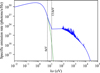 |
Fig. 1 Stellar spectrum adopted in our fiducial model. The vertical dashed lines mark the lower energy limits of the FUV and EUV bands. The lower limit of the X-ray band is 100 eV. (See also Table 1 for the integrated luminosities.) The thin green line shows the photospheric emission, which overlaps with the blue line below 6 eV, for reference. |
Simulation setup of the fiducial model.
2.2 Post-process
We post-processed the steady-state structures obtained from our simulations to generate synthetic intensity maps and fluxes for H2 pure rotational lines, specifically from S(1) to S(9) transitions. This involved calculating non-LTE H2 level populations and performing subsequent line radiative transfer using RADMC-3D (Dullemond et al. 2012).
The level populations are computed using the “Optically Thin non-LTE” method, appropriate for the typically optically thin nature of the H2 lines. Only collisional excitation, deexcitation, and spontaneous decay are considered. We neglect H2 pumping by UV, X-ray, and chemical reactions, though the hydrodynamics simulation includes FUV H2 pumping and chemical heating as heating sources (Section 2.1); the impacts of this simplification are discussed in Section 4.2. It is worth noting that while the population calculations do not incorporate line excitation or de-excitation, self-absorption is accounted for in the subsequent line transfer.
Molecular data for H2, including Einstein A coefficients and collisional rate coefficients for collisions with H, para-H2, ortho-H2, e−, and H+ (Roueff et al. 2019; Lique 2015; González-Lezana et al. 2021; Flower et al. 2000, 2021), are taken from the EMAA database1. In the post-processing, we input the density, velocities, temperature, H2 abundance, and the abundances of the collision partners obtained by the simulations. The para-H2 and ortho-H2 abundances are specified by assuming an ortho-to-para ratio of 3.
Unless otherwise noted, we assumed a distance to the source of d = 140 pc. We explored various disk inclinations and both dust-free and dust-obscured line emission cases.
For the fiducial case, we adopted an edge-on view (i = 90°) and neglected dust obscuration to isolate the intrinsic morphology and fluxes. This served as a baseline for comparisons.
Dust-obscured models use RADMC-3D's default silicate opacity and assume a dust-to-gas mass ratio of 0.01, which is about ten times higher than in the hydrodynamics simulation, to probe the upper-end effects of disk obscuration. Comparing these results with the dust-free case provides insight into the impact of intermediate dusty levels. Increasing dust opacity does not alter the thermochemical structures of the H2 winds in our simulation, so this treatment does not affect the internal consistency.
3 Results
We present the hydrodynamics simulation results and discuss the steady-state structures in Section 3.1, followed by an analysis of the system energetics in Section 3.2. Synthetic intensity maps and fluxes at i = 90° without disk obscuration are shown in Sections 3.3 and 3.4, respectively. Section 3.5 examines the density and temperature regimes traced by each line, followed by a rotation diagram analysis in Section 3.6. The effects of disk inclination and disk obscuration are addressed in Section 3.7. Finally, we discuss spectrally resolved line profiles from the models with disk obscuration in Section 3.8.
3.1 Properties of photoevaporative H2 winds
Figure 2 shows a snapshot of the hydrodynamics simulation after the system has reached a quasi-steady state at t ≈ 104yr. Photoevaporative H2 winds are evident in the third panel, where the blueish region marks the H2-dominated region, and white arrows indicate the velocity field. Advection plays a crucial role in shaping this H2 region, highlighting the importance to couple hydrodynamics with chemistry. The typical densities and temperatures of the H2 winds are 102 cm−3 ≲ nH2 ≲ 105 cm−3 and 100 K ≲ T ≲ 1000 K, respectively (the first and second panels). X-ray heating and H2 cooling dominate in the molecular region, while (hard) EUV heating and adiabatic cooling are more important in the atomic/ionic region.
When compared at a similar distance from the star, wind temperature generally anticorrelates with density: hotter winds are less dense. This is because softer X-rays and EUV, which have larger absorption cross-sections, are absorbed at lower column densities and have shorter heating timescales. Besides, atomic and molecular coolants tend to be more abundant at higher column densities and more efficient due to the higher densities. Since photoevaporative winds are pressure driven, higher temperatures generally lead to stronger acceleration and thus higher velocities. As a result, lower-density regions exhibit higher poloidal velocities (compare the top and bottom panels). The low-density wind component (nH2 ≲ 103 cm−3) is mostly supersonic, with poloidal velocities of vp ≳ 1 km s−1.
To examine how physical quantities evolve along the flow, Figure 3 presents their profiles along representative streamlines in the H I region (blue), near the H I/H2 boundary (red), and within the H2 region (cyan), launched at ≈3, 40, and 100 au, respectively. The profiles are plotted as functions of the streamline coordinate s, with s = 0 marking the base, defined as the point where the Mach number reaches M = 0.025 (see Appendix C for details). Figure 4 similarly shows the specific heating and cooling rates along the representative streamlines, including only the major contributing processes.
The flow near the H2 dissociation front (e.g., red streamline in Figure 3) originates from the disk surface at R ≈ 40 au, consistent with the critical radius at T ≈ 300 K. This gas travels roughly along the front, accelerating from <0.1 km s−1 to 4 km s−1 (Panel e). It takes ≈1000yr for this gas to exit the computational domain after leaving the disk surface. During the travel, gas density decreases monotonically from nH2 ≈ 105 cm−3 to ≈102 cm−3 (Panel c), while the temperature steadily increases from ≈102 K to 700 K over a distance of ≈ 100 au, and then levels off, nearly constant from that point to the outer computational boundary (Panel d). X-ray and EUV heating are the dominant heating processes (middle panel in Figure 4).
This gas is launched as fully molecular (Panel d), with H2 molecules gradually destroyed via X-ray photoionization as well as two X-ray-driven dissociation pathways. The first pathway (hereafter Path 1) involves proton transfer and dissociative recombination of hydrogen-bearing species: H2+ + H2 → H3+ + H, followed by H3+ + e → 3 H. In this sequence, H2+ is produced via X-ray photoionization, and two H2 molecules are destroyed per photoionization event. The second pathway (Path 2) proceeds through a series of ion-neutral and dissociative recombination reactions of oxygen-bearing ions: (i) H2 + OH+ → H2O+ + H, (ii)H2 + H2O+ → H3O+ + H, and (iii) H3O+ + e → OH + 2H. Here, OH+ in step (i) is generated through H+ + OH → OH+ + H and H2 + O+ → OH+ + H, where O+ is created via charge exchange, H+ + O → O+ + H.
The hydrogen ion is provided by X-ray photoionization H + hν → H+ + e (and to a lesser extent by ion-neutral reaction H + H2+ → H2 + H+). In total, three hydrogen molecules are destroyed per photoionization event, although this number effectively reduces to two when H2+ ends up with the ion-neutral reaction H + H2+ → H2 + H+. FUV photodissociation is negligible under the adopted stellar parameters.
The overall timescale of these dissociation processes is limited by the X-ray photoionization timescale (~3000yr). During the outflow, the H2 abundance drops from yH2 ≈ 0.5 (fully molecular) to yH2 ≈ 0.2 by the time the gas reaches the outer computational boundary, on a timescale of ≈ 1000 yr.
Gas launched beyond R ≈ 40 au remains largely fully molecular (e.g., cyan streamline in Figure 3). In this region, X-ray photoionization timescale increases rapidly with radius, due to both geometric dilution and absorption, outpacing the modest rise in the winds’ crossing timescales (see the fourth panel in Figure 2). The ionization timescale is ≳103 yr, yet X-ray photoionization remains a key H2 destruction process, along with the ion-neutral reaction H2+ + H2 → H3+ + H (Path 1).
Along streamlines, the H2 abundance gradually decreases by ~10% until leaving the computational domain on a timescale of ≈4000 yr. The gas density, temperature, and velocity follow similar trends to those found near the H2 dissociation front described above, albeit with less steep gradients (cyan lines in Figure 3). At these large distances, only X-ray heating remains effective due to the high column density, providing nearly all of the energy input (right panels in Figure 4).
In contrast, gas launched from within R ≈ 40 au undergoes substantial H2 depletion before being strongly accelerated (e.g., blue streamline in Figure 3). Here, the X-ray photoionization proceeds faster (≲103 yr), and the dominant destruction pathway shifts to the oxygen-bearing ion reactions (Path 2). In the innermost regions (a few au), the neutral-neutral reaction H2 + O→ OH + H also contributes, being efficient at high temperatures (activation energy ≈3150K). This inner atomic gas reaches T > 103 K (see the second panel of Figure 2), and shows steep gradients in density, temperature, and velocity along streamlines (blue lines in Figure 3). It attains the highest wind speed of ≈10 km s−1 and exits the computational domain within ~300yr. In this highly irradiated regime, energy losses via radiative cooling are negligible, and nearly all input energy is converted into the mechanical energy (left panels in Figure 4, and see also Figure C.2).
For reference, the cumulative mass-loss rates are estimated to be ≈1 × 10⁻⁹ M⊙ yr−1 in total (including helium), and ≈0.4 × 10⁻⁹ M⊙ yr−1 for H2. H2 accounts for nearly all hydrogen-bearing mass loss beyond ≳40 au, contributing about ≈70% of the total mass loss there. (See Appendix D and Figure D.1 for details).
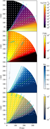 |
Fig. 2 Snapshot of H2 density (top), gas temperature (second), H2 abundance (third), and poloidal velocity (bottom). Cyan contours indicate isosurfaces for each quantity: nH2 = 10, 102, 103, 104, 105, 106, 107cm−3; T = 200, 500, 1000, 2000, 3000, 5000K; yH2 = 10−4,10−3,10−2,10−1; and vp = 1,2,5,10,20,30km s−1. In all panels, the white and green dashed contours denote the H2 dissociation front (yH2 = 0.25) and the isothermal sonic surface, respectively. White arrows indicate the velocity field (direction only, not its magnitude) and are omitted where T < 100K. In the H2 abundance map, the dotted gray contour marks the HI ionization front (yHII = 0.5). |
3.2 Energy budget
We examined the energetics of photoevaporative H2 winds, which can offer a useful diagnostic for assessing a photoevap-orative origin (Sections 4.1 and 4.4). The underlying principle is that in a photoevaporating system, a fraction of stellar UV and X-ray photons is absorbed and converted into heat, part of which is subsequently radiated away through H2 line emission. This leads to the energy constraint
 (2)
(2)
where LUVX is the total UV and X-ray luminosity; εheat(< 1) is the heating efficiency, defined as the fraction of LUVX converted into heat; and LH2 is the total H2 rovibrational line luminosity, or equivalently the total H2 cooling rate, from the UV- and X-ray-heated region.
In our model, LUVX = 3.9 × 1030 erg s−1, and the total luminosity is dominated by X-rays (Table 1). Integrating the rates of all photoheating processes throughout the computational domain yields a total heating rate of 1.6 × 1029 erg s−1, with X-rays, EUV, and FUV responsible for 1.1 × 1029 erg s−1, 4.7 × 1028 erg s−1, and 3.3 × 1027 erg s−1, respectively. This gives εheat = 4%, consistent with previous radiation hydrodynamics simulations reporting efficiencies of <10% (Wang & Goodman 2017; Wang et al. 2019).
The low efficiency reflects two main factors. First, only O(10%) of the emitted photons are actually absorbed. For instance, X-rays emitted toward low-polar-angle regions, where the column density is low (the dark areas in the top panel of Figure 2), escape the system with minimal absorption. Even in the H2 winds, where the column density is higher, not all photons are absorbed. Full attenuation occurs primarily along the boundary between the disk and wind regions, which subtends only a small solid angle from the perspective of the star.
Second, not all photon energy is converted into heat. A significant portion is lost to ionization and excitation. In the case of ionization, energy losses are substantial if photons have energies near the ionization potentials of the absorbers. For excitation, energy losses typically increase with the photoelectron’s energy (Shull & van Steenberg 1985; Maloney et al. 1996). For X-raygenerated photoelectrons, only ≈10% and ≈40% of the primary electron energy is converted into heat in the HI and H2 layers, respectively (Xu & McCray 1991 ; Maloney et al. 1996, see also discussions in Section 4.5). In the case of FUV photoelectric heating, typically <10% of the absorbed energy is converted into heat, and the efficiency can decrease further as the PAH and very small grain abundances reduce.
In our simulation, LH2 ≈ 1.3 × 1028 erg s−1, accounting for ≈9% of the total heating rate (εheatLUVX ≈ 1.6 × 1029 erg s−1, from X-ray, EUV, and FUV heating at 1.1 × 1029 erg s−1, 4.7 × 1028 erg s−1, and 3.3 × 1027 erg s−1, respectively), and thus LH2 ≈ 3.3 × 10⁻³LUVX. Strictly, LH2 includes contribution from the innermost region (≲3 au), where the gas temperature is maintained at ≳100K through dust-gas collisional heat exchange, indicating that the energy source for H2 emission is not limited to UV and X-ray irradiation, but also includes stellar optical radiation, which heats the dust grains. However, in our simulation, the contribution from this inner region is negligible compared to that from the UV- and X-ray-heated layers. It is therefore reasonable to consider UV and X-rays as the primary energy sources for LH2.
Note that our analysis does not account for energy absorbed within the inner boundary (≲1.8au). As such, the efficiencies derived here are applicable beyond ≈2au. For consistent comparison with observational estimates, the observed efficiency should likewise exclude contributions from within ≲2 au.
Additionally, while we find LH2 ≈ 3 × 10⁻³LUVX in the fiducial model, energy efficiency is generally luminositydependent, with typically more deposited energy going into total radiative cooling as luminosity increases (Nakatani et al. 2024). Caution is therefore advised when applying the derived efficiencies to sources with significantly different luminosities. We revisit this point in Section 4.3.
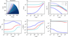 |
Fig. 3 Physical properties along streamlines. (a) H2 abundance map (same as Figure 2) with selected streamlines shown in gray. Three representative streamlines are marked in blue, red, and cyan. (b-f) Profiles of cylindrical radius, densities, temperature, poloidal velocity, and H2 abundance along the three streamlines, using consistent color coding. The horizontal axis indicates the distance along each streamline, with s = 0 defined at the base. In panel c, solid and dashed lines show H2 and hydrogen nucleus densities, respectively. |
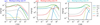 |
Fig. 4 Specific rates of major heating and cooling processes along the blue, red, and cyan streamlines in Figure 3, shown from left to right. Labels indicate: EUV photoionization heating (“EUV”); X-ray photoionization heating (“X-ray”); line cooling from O I, H2, and CO; and adiabatic cooling (“adi”). (See Figure C.2 in Appendix for the heating and cooling rates of other processes.) |
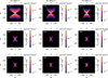 |
Fig. 5 Intrinsic morphologies of the H2 pure rotational lines (S(1)-S(9)) for a disk viewed edge-on (i = 90°) without disk obscuration. The colors indicate the frequency-integrated intensities, with individual color bars scaled independently in each panel, Right ascension and declination offsets are shown assuming a source distance of d = 140 pc. |
3.3 Intrinsic H2 line intensity maps
In this section, we present the integrated intensity maps, postprocessed with RADMC-3D, to examine the morphology of photoevaporative H2 winds, one of the central focuses of this study. We first analyze the case with i = 90° and no disk obscuration, which reveals the intrinsic emission structure and fluxes. This serves as a reference for more observationally realistic scenarios with different inclinations and disk obscuration, discussed later in Section 3.7.
Figure 5 displays the frequency-integrated intensity maps for the H2 S(1)-S(9) lines, all exhibiting an X-shaped morphology with a central emission peak. The X-shaped structure originates from warm H2 gas (≳100K; see Figure 2), where thermal excitation is efficient. The X-arms trace regions of peak column density in an edge-on view, extending outward with slight collimation and a convex curvature, i.e., the semi-opening angle narrows with increasing distance. This morphology reflects the underlying temperature and H2 distributions (second and third panels in Figure 2).
The emission becomes increasingly compact and slightly more collimated from S(1) to S(9), reflecting the underlying density distribution and the radial and angular temperature gradients. Higher excitation lines require higher densities and trace hotter gas, which resides at smaller radii and lower polar angles (second panel of Figure 2).
The central emission peak originates from the hot, high-density atmosphere of the inner disk (r ≲ 3 au). Note that our computational domain excludes r ≲ 1.8 au where hot, even denser atmosphere likely exists, so the peak emission may be underestimated.
To quantify the morphology, Table 3 lists three key metrics of the images in Figure 5: (i) the emission extent rext, defined as the radius enclosing 95% of the total flux; (ii) the geometric radius Rgeo, where a linear fit to the wind emission intersects the disk midplane, following Pascucci et al. (2025); (iii) the semi-opening angle θopen, defined as the polar angle where the emission peaks at each radius. Since θopen varies with the radius, Table 3 reports both the mean value θ̄open and a log-linear fit: θopen = θ0-θ1 log(r/100 au). The fit uses data from r > 20 au to exclude the inner region. For consistency with Pascucci et al. (2025), Rgeo is measured using points ~0.2" above and below the midplane. Overall, rext and θ̄open decrease with decreasing wavelength. Rgeo also decreases for S(2)-S(9), although S(1) shows a further drop due to its distinct emission geometry (see Figure 5).
To evaluate point spread function (PSF) effects on the geometric indicators, we also measured rext, Rgeo, θopen from images convolved with 2D Gaussians. The FWHMs were set to 0."033(λ/1 μm) + 0.″106 for S(1)-S(8) (Law et al. 2023) and 0.″21 for S(9), estimated using a STPSF simulation tool (Perrin et al. 2014). For Rgeo and θopen, we excluded emission from the inner region (r < 20 au) before convolution to isolate the wind component.
Generally, PSF convolution blurs the convex shapes of the emission, making the morphology appear more as a straight X-shape (Figure 6). This is also reflected in the smaller absolute values of “cnv.” θ1 than the “int.” ones in Table 3.
For θ̄open, the convolution results in a systematic reduction, due to contributions from emission between the arms of the X-shape. The reduction θopen is more significant at smaller radii (r ≲ 50 au), while at larger radii, θopen is mostly unchanged from the intrinsic values.
For Rgeo, the convolution decreases the value across all lines in our model. The negative Rgeo for S(1) originates from the convolution causing the emission peak at each radius to shift systematically upward above the midplane and inward toward the rotational axis, especially within ≲100 au. Near the central region, the convolution mixes contributions from both the arms of the X-shaped structure. The relatively large opening angle further contributes to producing a negative Rgeo. Similar effects are also responsible for the small Rgeo measured in the convoluted S(2) image.
To summarize, PSFs can significantly alter the geometric indicators. Accounting for these PSF-induced biases is essential when interpreting wind-launching points or inferring winddriving mechanisms from morphology.
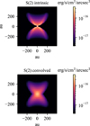 |
Fig. 6 Comparison of emission morphologies between the intrinsic and Gaussian-convolved S(2) images. Top panel: original image from Figure 5. Bottom panel: same image convolved with a Gaussian kernel of FWHM ∼72 au. |
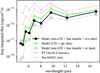 |
Fig. 7 Integrated fluxes of the S(1)-S(9) lines for the model with i = 90° without disk obscuration and assuming d = 140 pc (black dots). For reference, green crosses indicate the fluxes calculated under the assumptions of LTE and optically thin emission. Observed fluxes for SY Cha (blue; d = 180.7 pc) and Tau 042021 (red; d ~ 140 pc) are also shown for comparison. For SY Cha, we adopted the fluxes measured with a radius aperture of 0.5-2″. Since the spatial integration regions differ between our model and the observations of Tau 042021, and the SY Cha fluxes are not scaled by distance, care should be taken when making direct comparisons (see also Sections 4.4.1 and 4.4.2 and Figure 14). Open circles correspond to the model fluxes with i = 90° but including disk obscuration (Section 3.7; Table 5). |
3.4 H2 line fluxes
Now we turn to the integrated fluxes derived from the intensity maps (Figure 5), which - alongside morphology - represent a key focus of this paper. Figure 7 shows the integrated fluxes (black filled dots) as a function of wavelength, with corresponding values listed in Table 2 with d = 140 pc. The S(1)-S(5) lines, which exhibit extended emission, have fluxes on the order of 10−16−10−15 erg s−1 cm−2. Higher J lines - emitted primarily from the hot, high-density atmosphere of the inner disk (r ≲ 3 au) - are more compact in emission and show fluxes about an order of magnitude lower.
All lines are generally optically thin; only S(1) becomes marginally optically thick near the center, but this has a minimal impact on the image and flux. Most emission arises from the regions close to LTE, making the optically thin plus LTE approximation reasonably accurate.
This is supported by the green crosses in Figure 7, which mark the fluxes computed under the LTE and optically thin assumptions. These fairly agree with the full non-LTE radiative transfer results (black filled dots) within a factor of two across all lines.
For comparison, observed fluxes of Tau 042021 (d ~ 140 pc Arulanantham et al. 2024) and SY Cha (d ≈ 180.7 pc Schwarz et al. 2025a) are also shown (see also Table 2). The overall agreement, especially for lower J lines, is striking. However, we note that the spatial integration domains used to derive the Tau 042021 fluxes are smaller than those in our model, and that the SY Cha fluxes are shown as raw values, without scaling by the distance of d = 180.7 pc. A more detailed comparison follows in Sections 4.4.1 and 4.4.2.
3.5 Gas properties traced by each line
To probe the physical conditions traced by each line, we defined a convenient diagnostic quantity, referred to as the local integrated luminosity,

where νul and Aul are the frequency and Einstein A-coefficient for the J + 2 → J transition, and nu is the upper-level population. This quantity represents the line luminosity contribution from a volume element spanning uniform intervals in ln r, θ, and ϕ.
The physical meaning of LJ may become clearer in its volume-integrated form. Assuming optically thin emission, the integrated line flux is expressed by

so LJ approximately indicates the relative contribution of gas at (r, θ) to the optically thin total flux FJ (or equivalently, the intrinsic total line luminosity). Mapping LJ onto a densitytemperature phase diagram provides the physical conditions traced by each line. We note that LJ and FJ are diagnostic quantities introduced to identify the regions that contribute most to the optically thin total line luminosity and flux, and thus generally differ from those obtained through radiative transfer calculations. However, they become physically equivalent when the line is optically thin and dust extinction is negligible.
Figure 8 shows scatter plots of normalized LJ for each computational cell using the non-LTE level populations computed with RADMC-3D. The dark red-violet points highlight the combinations of nH2 and T contributing predominantly to each line. In general, emission originates from two components: the hot, high-density atmosphere of the inner disk and the more extended, lower-density photoevaporative winds. This dual contribution is consistent with the intensity maps in Figure 5, which show the brightest emission at the center with the extended diffuse emission.
These two regions are roughly separated at r ≈ 3-7 au. For S(5)-S(9), the disk component arises primarily from r ≲ 3 au. We again note that our computational domain excludes the innermost region (r ≲ 1.8 au).
Focusing on the wind (nH2 ≲ 105 cm−3 on the scatter plots), we find that higher excitation lines trace hotter and more rarefied gas. The contributing conditions range from (nH2, T) ~ (105 cm−3,300K) for lower J lines to ~(102 cm−3,900K) for higher J lines. Broadly, the S(1)-S(3) lines primarily trace cooler gas T ~ 200-103K, while the S(4)-S(9) lines are sensitive to warmer regions 700 K ≲ T ≲ 2000 K. Higher temperatures imply higher sound speeds and faster photoevaporative winds. This is visualized by the black contours in Figure 8, which mark poloidal velocities: S(1)-S(3) emission arises in part from slow wind components (~1 km s−1; see Figure 2), while S(4)-S(9) are predominantly associated with faster-moving gas.
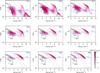 |
Fig. 8 Phase-space scatter plots of the normalized local integrated luminosity LJ/LJ,max for each H2 line. Each point corresponds to a computational cell in the simulation, with point size scaled by LJ/LJ,max to reduce overlap and emphasize more emissive regions. The reddish areas highlight the densities and temperatures ranges that most strongly contribute to the total emission. Solid black lines mark approximate contours of poloidal wind velocity (vp = 1, 3, and 5 km s−1), and the green contour indicates the isothermal sonic surface. Dashed blue lines represent the best-fit rotational temperatures (Table 4). |
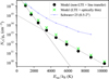 |
Fig. 9 Rotation diagram of the H2 lines. Black dots show the model results from non-LTE calculations with line transfer using RADMC-3D. The solid and dashed black lines are a two-component fit to the lower J lines S(1)-S(3) and the higher J lines S(4)-S(9), respectively. Green crosses indicate the values assuming LTE and optically thin emission -i.e., the maximum emission possible within our model setup. For reference, observational data for SY Cha are shown with a blue line (Schwarz et al. 2025a). Since the emitting area is not specified in Arulanantham et al. (2024), the data for Tau 042021 are omitted to avoid introducing additional uncertainties. |
3.6 Rotation diagram analysis
We performed a rotation diagram analysis to assess how well the physical properties of photoevaporative H2 winds can be inferred from observations. We then compared the derived temperatures and H2 column densities with those in the simulation.
The analysis fit the integrated fluxes FJ, which are determined by solving radiative transfer, as a function of Eup using

Here,  , gu is the statistical weight, Q is the partition function, Trot is rotational temperature, N̄H2 is the average H2 column density over the emitting region with solid angle Ω.
Figure 9 shows the resulting rotation diagram (black points). We fit the data in two ways: using all transitions S(1)-S(9), and using a two-component approach that divides lower J S(1)-S(3) and the higher J S(4)-S(9) lines. We find that the two-component fit provides a better fit. This reflects the presence of multiple temperature components in the wind, as discussed in Sections 3.1 and 3.5. Figure 9 only shows the two-component fit for clarity.
The best-fit parameters are listed in Table 4. While the level populations are not strictly in LTE, the derived Trot provides reasonable estimates for the temperatures traced by the lower and higher J lines (compare the horizontal blue dashed lines and reddish regions in Figure 8). Similarly, the best-fit NH2 agree well with simulation values: N̄H2 = 3.3 × 1018 cm−2 for 200 K ≲ T ≲ 103K, and 3.7 × 1016 cm−2 for T ≥ 700 K. These agreements are non-trivial, given the non-LTE nature of the emission, but are expected: most emission arises from regions where LTE is a good approximation.
We note that our two-component fit differs slightly from the method used in Schwarz et al. (2025b), where S(1)-S(8) fluxes are fitted simultaneously. This approach does not require pre-defining the boundary between warm and hot components; instead, it naturally emerges from the fit. Applying this technique to our fluxes yields a slightly higher hot-component Trot (≈900 K) because S(4) contributes to both components, lowering the flux attributed to the hot component relative to our segmented two-component fit. This highlights the need for caution when selecting line ranges in a segmented two-component fit to ensure consistency with simultaneous fitting methods.
Comparison of model fluxes for different inclinations with and without disk obscuration.
3.7 Effects of inclination and disk obscuration
From Section 3.3 onward, we have focused on an edge-on disk (i = 90°) and without disk obscuration. Here, we explore how inclination and dust extinction within the disk affect the results.
Inclination alone has little effect on the integrated line fluxes in the absence of disk obscuration, as the emission is optically thin (Section 3.4). Indeed, the fluxes remain nearly constant across inclinations (Table 5), except for a slight increase in S(1) at lower inclinations due to marginal optical thickness at the center. We note that this holds for emission beyond ≳2 au, the region covered by our simulation; stronger inclination dependence may appear for inner regions where intense H2 emission is expected from denser disk atmosphere.
Disk obscuration significantly reduces the flux by obscuring the central and/or far-side regions, depending on viewing angle. For nearly edge-on disks, the midplane is obscured, forming a dark lane and leaving only the vertically extended emission visible, in particular for S(1)-S(3) (Figure 10). This results in a flux reduction by a factor of a few for S(1)-S(6) and by a larger factor for higher J lines S(7)-S(9) (Table 5). The stronger suppression of higher J lines reflects their origin in the hot inner disk atmosphere.
Even reducing the dust-to-gas mass ratio to 0.0015 in the disk only modestly increases the flux: a factor of two for S(9) and less than 50% for the other lines. Compared to the observed fluxes, our model significantly underpredicts the higher J line fluxes (S(7)-S(9)) in the dust-obscured case, though lower J lines remain in relatively good agreement (Figure 7 and Table 2). This suggests that our model may underestimate the higher J line emission from the extended wind component. We revisit this possibility in Section 4.2.
In less inclined disks (e.g., i = 60°; Figure 11), attenuation primarily affects the far side of the disk. This is most noticeable in the S(3) image, where the far-side emission is mostly obscured, due to the silicate opacity enhancement near ≈10 μm. For lower J lines, the morphology shifts from X-shaped to more bowl-shaped with decreasing i.
Flux reductions with respect to the dust-free case vary across transitions, but remain relatively modest - less than a factor of two for all lines (Table 5). Even the higher J lines are only moderately impacted, since the inner emitting regions are not completely obscured.
To summarize, while the morphology transitions from X-shaped (edge-on) to bowl-shaped (face-on), inclination has minimal impacts on the fluxes unless disk obscuration is significant. Dust obscuration becomes important in edge-on systems, leading to: (1) a dark lane in images, (2) corresponding flux reduction for high J lines such as S(7)-S(9) by obscuring emission from the hot inner disk atmosphere. For face-on to moderately inclined disks, the effects are minimal; flux reduction is less than a factor of two.
Given that we may underestimate extended high J emission (Section 4.2), the actual impact of inclination and dust obscuration could be even smaller in real systems. We emphasize that these conclusions apply beyond ≳2 au; emission from the inner regions inside our computational boundary may exhibit a stronger dependence on inclination and disk obscuration. The results also depend on the adopted dust opacity and the degree of settling, and therefore the trends should be interpreted qualitatively.
While edge-on sources help probe wind geometry (e.g., its semi-opening angle), disks at all inclinations may offer comparable insights for the physical conditions of photoevaporative H2 winds. Moderately inclined disks would be particularly advantageous, as they enable complementary comparisons with stellar X-ray and UV luminosities, key diagnostics for photoevaporation (Section 4.1).
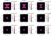 |
Fig. 10 Same as Figure 5, but including dust extinction within the disk. The panels show continuum-subtracted images. |
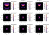 |
Fig. 11 Same as Figures 5 and 10 but for an inclination of i = 60° including dust extinction within the disk. |
3.8 Velocity profiles
We generate spectrally resolved, continuum-subtracted line spectra, using the images of the fiducial model with inclinations of i = 0, 30,45,60,90°. The spectral window spans ±30 km s−1 around the line centers and is sampled with 201 wavelength points (corresponding to a spectral resolution of R ≈ 106). In producing the spectra, we manually exclude emission from the far side of the disk for inclined cases (i < 90°), to isolate the contribution from the near-side surface. The resulting velocity profiles for selected lines are shown in Figure 12.
Overall, low J lines (S(1)-S(4)) exhibit blueshifted, singlepeaked profiles, reflecting strong contributions from the extended wind component. For higher J lines (S(5)-S(9)), emission from the hot, dense atmosphere of the inner disk (R ≲ 3 au) becomes relatively significant (see Sections 3.3 and 3.5). At i < 90°, this leads to high-velocity wings (|v| ≳ 10 km s−1) produced by Keplerian motion in the inner disk atmosphere. At intermediate inclinations (i = 30-60°), the high J line profiles appear flatter and multi-peaked. However, this may partly reflect underestimated high J emission from the extended wind (see also Section 4.2); including it could yield single-peaked, brighter profiles, suppressing the flatter structures. The profiles in Figure 12 also exclude the contribution from the innermost region (≲2au), which is outside our computational domain, and should therefore be interpreted as those arising from the outer disk.
The velocity centroids vcent are generally small (|vcent| ≲ 1 km s−1) across all lines. The FWHMs of single-peaked lines increase with higher J, ranging from 3 km s−1 to 8 km s−1, and broaden slightly with inclination up to i ≈ 60° (by only a factor of ≈1.5), remaining nearly constant at higher inclinations i ≳ 60°. These small |vcent| and narrow widths highlight the slow nature of photoevaporative winds launched from outer radii (Section 3.1) and imply that resolving their kinematics is inherently challenging, even at the highest spectral resolutions (R ≈ 100000; ∆v - 3 km s−1) achievable with current and future instruments such as VLT/CRIRES+ and ELT/METIS.
While vcent below the instrumental resolution can in principle be measured with sufficient signal-to-noise ratio (S/N), detecting a ~1 km s−1 shift at R ~ 100000 requires S/N ≳ 10. CRIRES+ covers the S(8) and S(9) lines and can reach S/N ≈ 10-20 at the line centers with a few-hour integration time, assuming a typical FWHM of ~ 3 km s−1 and line fluxes of ≈10−15 erg s−1 cm−2 for the wind component (see SY Cha fluxes). However, these high J lines may also have substantial contributions from the inner hot disk (Schwarz et al. 2025a), requiring high spatial resolution as well to isolate the wind component. Future > 30 m-class telescopes, like ELT/METIS, will be particularly valuable for disentangling the kinematic signatures of winds to probe their origins.
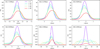 |
Fig. 12 Velocity profiles of selected lines viewed at inclinations of i = 0° (purple), 30° (cyan), 45° (light green), 60° (yellow), and 90° (red). For i < 90°, the profiles were computed excluding emission from the far side of the disk, isolating the contribution from the near-side surface. |
4 Discussion
In Section 4.1, we recap our main findings and discuss observational diagnostics of photoevaporative winds. Section 4.2 examines the potential impacts of pumping processes on our results. We then explore how the findings may vary with different stellar properties, such as mass and UV/X-ray luminosities, in Section 4.3. In Section 4.4, we compare our models with recent JWST observations and assess whether the observed H2 winds can be explained by photoevaporation, in light of preceding results. Finally, we highlight key caveats in Section 4.5.
4.1 How to tell whether observed H2 winds are photoevaporative or not
Photoevaporation drives H2 winds with a curved dissociation front. The winds typically have H2 densities of 102−105 cm−3 and temperatures of 100-1000 K with the fiducial parameters. This structure results in an X-shaped morphology in the S(1)-S(9) emission when viewed edge-on (Figure 5). The spatial extent of the emission decreases for higher J, from ~300au to ~50au, though the latter may be underestimated (see Section 4.2). The semi-opening angle also decreases for higher J, from ~50° to ~37°, comparable to values observed in Tau 042021 and SY Cha. This suggests a photoevaporative origin remains plausible for these sources, contrasting to the current interpretation favoring MHD winds. Our model demonstrates that geometric indicators such as opening angles and spatial extent are not definitive diagnostics unless the wind is extremely collimated. Given the PSF-induced biases (Section 3.3), caution is essential when using these indicators to estimate wind-launching points or infer wind-driving mechanisms.
Energetics offer a more robust constraint. As discussed in Section 3.2, only ≲10% of the stellar UV/X-ray luminosity is converted into heat, and a small fraction of that (≈9% in our model) is radiated away as H2 emission. This sets an empirical necessary condition for a photoevaporative origin: the observed H2 line luminosity needs to satisfy LH2 ≲ 0.01 LUVX (in our simulation, LH2 ≈ 3 × 10⁻³LUVX). Exceeding this implies an additional energy source, such as accretion powering MHD winds. Note that this condition applies beyond ≳2 au, as our model excludes energy absorbed closer in; observed efficiencies should be evaluated consistently. Also, this criterion considers only H2 emission from thermal excitation. In practice, higher J levels can be significantly influenced by nonthermal processes (Section 4.2). Therefore, LH2 should be evaluated using lower J lines (e.g., S(1)-S(3)), which have low critical densities. Even when all lines are included in estimating LH2, the total H2 luminosity would still remain below ≲0.1 LUVX, a hard limit for photoevaporative winds, given that only O(10%) of the UV and X-ray luminosity is typically absorbed by the wind (noting again that not all of the absorbed energy is converted into heat, as discussed in Section 3.2).
Wind velocity provides another criterion. Photoevaporative H2 winds typically have poloidal velocities of ~1-5 km s−1. If the H2 emission arises from H I-dominated regions, velocities may reach ≈10 km s−1 but not significantly beyond such speeds, as acceleration is limited past the isothermal sonic point. Thus, a velocity threshold of ≈10 km s−1 serves as a practical upper bound. Accordingly, velocity centroids are expected to remain below this limit, typically on the order of 1 km s−1. In contrast, MHD winds can exceed this range. In the cold MHD wind regime, the asymptotic velocity is given by  , where vK is the Keplerian velocity, R0 is the launching radius, and λ is the magnetic lever arm parameter (Blandford & Payne 1982). For λ ~ 2-5 (e.g., Tabone et al. 2017; Louvet et al. 2018; Gressel et al. 2020; Lesur 2021; Kadam et al. 2025), this yields v∞ - 10-25 km s−1 at R0 ~ 10 au for M* = 1 M⊙. In the magneto-thermal wind regime, where the lever arm is minimal and acceleration is driven primarily by pressure gradients, the radial velocities are typically ≲5 km s−1 (Bai 2017; Wang et al. 2019).
In summary, key necessary conditions for photoevaporative winds include moderately wide opening angles (see θopen ≈ 30°-50° in the current model), an energy budget satisfying LH2 ≲ 0.01 LUVX, and wind velocities ≲10 km s−1. While such low velocities are very challenging to resolve with JWST, morphology and energetics provide a strong diagnostic framework. These criteria would not rule out MHD winds, but their interpretation remains uncertain without detailed predictions from MHD models.
A systematic survey correlating H2 flux with both UV and X-ray luminosities would be valuable. Moderately inclined disks are optimal targets, enabling both morphological analysis and comparisons with stellar UV/X-ray luminosities. As we discuss later in Section 4.3, for low accretors like the one assumed in the fiducial model, X-rays can dominate the energy input and scale with LH2 (Sections 3.1 and 3.2). For FUV-dominated sources, trends remain unclear: lower J fluxes (e.g., S(1)-S(4)) may weakly anticorrelate with LFUV due to enhanced H2 photodissociation, while for higher J lines, H2 photodissociation and excitation by nonthermal processes (e.g., UV pumping) may compete, making the correlation nontrivial. Further investigation is warranted from theoretical perspectives.
4.2 Missing extended high J line emission
As discussed in Section 3.7, our model has likely underpredicted higher J line fluxes, especially for S(7)-S(9). Morphologically, our model also predicts smaller radial extent than observed for the higher J lines (Schwarz et al. 2025b; Pascucci et al. 2025). In this section, we examine whether these discrepancies could rule out a photoevaporative origin, or if they instead point to missing physical processes in the current model that might enhance extended high J emission.
These discrepancies can arise from simplifications in our treatment of the level populations. Specifically, we omit UV and X-ray pumping, as well as H2 excitation upon formation (hereafter formation pumping or chemical pumping)2, both of which can populate excited rovibrational levels. Another possible factor is our neglect of emission from the inner, hotter disk outside our computational domain that is scattered by dust at larger radii. We assess whether these processes could reconcile the discrepancies between our model and observations.
Regarding UV pumping, absorption in the Lyman and Werner bands (≳11.2 eV) excites H2 molecules to electronic excited states, followed by radiative decay into excited rovibra-tional levels of the electronic ground state. To assess whether UV pumping significantly enhances pure rotational level populations, we have performed one-zone level population calculations using the Paris-Durham code (Flower & Pineau des Forêts 2003; Godard et al. 2019), which can compute H2 level populations for given density, temperature, and UV field strength. We adopted physical conditions representative of the H2 wind near the dissociation front at r ~ 200 au, where our model appears to underpredict high J emission. Relevant parameters center around nH ~ 103 cm−3 (nH2 ~ 102−103 cm−3) and T ~ 600-900K.
We find that the impact of UV pumping on pure rotational excitation sensitively depends on the treatment of formation pumping, across a broad parameter space, nH = 1-104 cm−3, T = 500-2000 K, and G0 = 1-103. In the standard setup of the shock code, formation pumping follows a Boltzmann distribution at Tex = 17 249 K. Under this assumption, UV pumping has minimal effect on pure rotational levels, consistent with previous studies of irradiated interstellar gas (Black & van Dishoeck 1987; Godard et al. 2019) and protoplanetary disks (Nomura & Millar 2005; Nomura et al. 2007). Even for high J levels (J = 7-11), the enhancement from UV pumping is typically within a factor of two.
In contrast, if instead H2 is assumed to form only in the lowest levels ((v, J) = (0,0), (0,1)), corresponding to level population calculations in this study, UV pumping becomes the sole channel for populating higher levels. This leads to order-of-magnitude increases in the populations of high J pure rotational levels, particularly for J ≳ 7-8, when G0 ≳ 10. Even at G0 = 1, significant increases are seen in low-temperature, low-density gas, where collisional excitation is inefficient.
These results suggest that formation pumping, alongside UV pumping, plays a critical role in setting high J populations, particularly for J ≳ 7-8. Incorporating these processes could improve agreement with the observed high J fluxes and morphologies, indicating that the discrepancies do not rule out a photoevaporative origin. A detailed treatment, however, lies beyond the scope of this work and will be addressed in future modeling efforts.
The strong enhancement of populations due to formation pumping contrasts with the case of vibrationally excited states, such as the lowest-J levels at v = 1, where UV pumping is typically more effective, even though their excitation energies are comparable to those of pure rotational levels at J ≈ 8. This highlights the importance of including UV pumping when modeling vibrationally excited lines, such as the v = 1-0 S(1) line at 2.12 μm, which is commonly used to trace winds (e.g., Gangi et al. 2020; Pascucci et al. 2025). This line has also been found to be spatially extended, similar to the pure rotational S(9) emission (Pascucci et al. 2025). More recently, Kalscheur et al. (2025) have proposed FUV fluorescent lines as additional wind tracers. Together, these findings reinforce the need to incorporate UV pumping for testing models.
Similar to UV pumping, X-ray absorption can also excite H2 to rovibrational levels. Energetic photoelectrons produced by X-ray ionization can collisionally excite ambient H2 into electronically excited states, which then decay into various rovibrational levels of the ground electronic state (Gredel & Dalgarno 1995). These photoelectrons can also directly excite the molecules vibrationally, as they lose energy through collisions. Nomura et al. (2007) modeled these effects, along with UV and chemical pumping, in a hydrostatic disk and found little enhancement in pure rotational level populations, possibly because chemical pumping dominates rovibrational excitation. Thus, the impact of X-ray pumping is expected to be similar to that of UV pumping.
As for the potential contribution of infrared line scattering on small dust in the wind, its effect on high J emission appears minor, although some uncertainty remains. Schwarz et al. (2025b) showed that the extended H2 emission in SY Cha lies well above the flat scattered-light surface imaged by SPHERE at 2.2 μm, suggesting that scattering is unlikely to be a major factor in this system. In Tau 042021, S(5)-S(8) emission appears spatially coincident with 5 μm dust emission (Arulanantham et al. 2024), whereas S(9) emission seems spatially offset from it (Pascucci et al. 2025). Overall, we expect the contribution of scattering to high J emission to be small. This would especially be the case for photoevaporative winds given the generally dust-optically thin nature.
4.3 Stellar parameter dependence
The properties of photoevaporative winds are generally sensitive to stellar UV and X-ray luminosities, which can strongly influence H2 emission. Here, we explore how varying these luminosities affects the morphologies and fluxes of the H2 lines, relative to our fiducial model. We also briefly consider the role of stellar mass. These tests provide context for our comparison with the observations in Section 4.4. They also highlight the potential of using correlations between H2 emission and stellar properties as a diagnostic of photoevaporation.
As LFUV increases, line emission is expected to strengthen due to enhanced heating. However, H2 also becomes more susceptible to FUV photodissociation, particularly in low-density, high-temperature regions (T ≳ 500 K), making the net effect on the fluxes nontrivial. Additionally, higher LFUV broadens the H2 dissociation front, increasing the semi-opening angle.
To assess this, we restarted the fiducial simulation with higher FUV luminosities, LFUV = 4.0 × 1030 erg s−1 and 3.5 × 1031 erg s−1 (4 times and 40 times the fiducial value), corresponding to Ṁacc = 10−9 M⊙ yr−1 and 10−8 M⊙ yr−1, respectively. All other parameters remained the same as in Table 1. In these runs, FUV photodissociation contributes to H2 destruction at levels exceeding or comparable to those from X-ray photoionization in the fiducial model.
In the four times FUV case, the overall disk structure is similar to the fiducial model (Figure 2), but enhanced FUV photodissociation destroys hot H2 near the dissociation front, reducing the vertical extent of high J emission, and slightly broadening the semi-opening angles to θ̄open ≈ 40°-46°. Line fluxes decrease by a factor of a few (compare yellow and black lines in the top panels of Figure 13). The energy efficiency is also correspondingly reduced to LH2 ≈ 0.93 × 10⁻³LUVX.
These trends are more pronounced in the 40 times FUV run. X-ray heating remains dominant throughout most of the H2 region, except near the wind base where FUV photoelectric heating becomes comparable. The main effect of stronger FUV is enhanced destruction of warm H2 (T ≳ 300 K). The overall temperature structure changes little but is slightly reduced due to increased cooling by O I, whose abundance rises following stronger CO photodissociation. These effects collectively lead to weaker H2 line fluxes (pink lines in the top panels of Figure 13). When disk obscuration is included for an edge-on geometry (pink line in the top right panel), the depletion of warm H2 further reduces fluxes from the extended H2 winds. The resulting energy efficiency is even lower at LH2 ≈ 1.3 × 10⁻⁴LUVX.
We also tested enhanced X-ray luminosities of LX = 2.82 × 1031 erg s−1 and LX = 2.82 × 1032 erg s−1 (10 times and 100 times the fiducial value; the latter for experimental purposes). At ten times the fiducial value, line fluxes increase across all transitions (thick green lines in Figure 13), and the semi-opening angles widen to θ̄open ≈ 45°-55°. High J emission remains compact, leaving unresolved the issue discussed in Section 4.2. At 100 times, fluxes rise further (thick blue lines in Figure 13) and opening angles reach θopen ≈ 50°-60°. These trends reflect faster H2 destruction and more efficient heating of denser H2 layers at higher LX. The energy efficiency is comparable to the fiducial model: LH2 = 5.2 × 10⁻³LUVX and 4.8 × 10⁻³LUVX for the 10 times and 100 times runs, respectively. The relatively higher efficiencies, compared to the high LFUV models, indicate greater energy deposition per H2 molecule destruction.
In summary, both H2 morphology and fluxes are sensitive to UV and X-ray luminosities. Our preliminary results reveal overall trends: line fluxes increase with higher LX and lower LFUV, while semi-opening angles grow with both. However, the decreasing trend of high J line fluxes (e.g., S(5)-S(9)) with increasing LFUV is uncertain - if UV and chemical pumping were included, higher LFUV could instead enhance high J emission. Moreover, the results from the high FUV runs should not be interpreted as implying that H2 winds cannot be reproduced in systems with strong FUV radiation, as variations in PAH and elemental abundances may also play a role (Section 4.5). These results simply illustrate relative trends when either the FUV or X-ray luminosity is held fixed. A systematic parameter study is therefore needed to verify these trends and fully map the range of fluxes and morphologies that photoevaporative winds can produce. Our current findings suggest that photoevaporative H2 winds are more readily detectable in evolved disks around low-mass, active stars with low accretion rates (particularly in low J lines).
Stellar mass can also influence wind geometry. For instance, stars with M* < 1 M⊙ may produce narrower semi-opening angles than our fiducial model, as H2 can be launched from smaller radii and the disk scale height increases due to weaker stellar gravity. This trend contrasts with the broader semiopening angles seen under stronger UV and X-ray irradiation, suggesting that different combinations of M*, LX, and LFUV could result in similar wind morphologies.
To test this, we ran a model with M* = 0.4 M⊙ and ten times the fiducial X-ray luminosity (with L* = 0.93 L⊙ and R* = 2.12R⊙). We chose this setup, as it is expected to most closely reproduce the morphology in the fiducial model, based on the preceding exploration. Indeed, this model yields a similar morphology to the fiducial run (see also the discussion in Section 4.4.1). The H2 line fluxes are comparable to those in the ten times X-ray run (see the light green lines in the top panels of Figure 13).
These preliminary findings reinforce our argument in Section 4.1 that, without well-constrained stellar properties, geometric structure alone is insufficient to distinguish between photoevaporation and MHD winds. A systematic exploration of both stellar mass and luminosities is therefore essential for robust interpretation. On the theoretical side, these variations of morphology and fluxes indicates the need of source-specific modeling in conclusively assessing the origin of observed H2 winds.
4.4 Comparisons with JWST observations
The characteristic X-shaped morphology of the H2 emission in our model images (Figure 5) resembles recent JWST observations of Tau 042021 (Arulanantham et al. 2024) and SY Cha (Schwarz et al. 2025b), prompting the question of how well our photoevaporation model can quantitatively reproduce these features. In this section, we address that question. Comparisons with Tau 042021 (Arulanantham et al. 2024) and SY Cha (Schwarz et al. 2025b) are presented in Sections 4.4.1 and 4.4.2, respectively.
4.4.1 Tau 042021
Tau 042021 (2MASS J04202144+2813491) features an edge-on disk around an M-type star in Taurus (Luhman et al. 2009; Stapelfeldt et al. 2014; Simon et al. 2019). The disk inclination is i > 85° (Villenave et al. 2020), and the stellar mass is M* = 0.4 M⊙ (Duchêne et al. 2024)3. The accretion rate is estimated at Ṁacc = 2 × 10⁻¹¹ M⊙ through hydrogen recombination lines (Arulanantham et al. 2024), though this likely underestimates the true value due to the nearly edge-on orientation. In fact, Bajaj et al. (2025) report a much higher accretion rate Ṁacc ~ 10−8 M⊙ yr−1 based on jet mass-loss rates.
Recent ALMA observations in Bands 4 and 7 have resolved the disk’s vertical structure, revealing strong settling of large grains (Villenave et al. 2020). Meanwhile, JWST/MIRI imaging at 7.7 μm and 12.8 μm has revealed a prominent X-shaped structure extending above the midplane (Duchêne et al. 2024). This X-shaped emission lies above the warm molecular 12CO layer traced by ALMA, which has a semi-opening angle of θ̄open ~ 55° and vertical extent reaching up to ~225 au.
More recently, Arulanantham et al. (2024) detected the H2 S(1)-S(8) lines with JWST/MIRI. The S(2) image (12.3 μm) exhibits a clear X-shaped morphology, consistent with earlier 7.7 μm and 12.8 μm data of Duchêne et al. (2024), and may in part be traced by vertically extended 12CO (Foucher et al. 2025). The S(1)-S(4) lines are similarly vertically extended beyond the scattered-light continuum, whereas S(5)-S(8) appear more compact and cospatial with dust emission at 5 μm.
The semi-opening angle from the S(2) line is θ̄open = 35° ± 5°, which Arulanantham et al. (2024) interpret as evidence of a MHD wind. They cite its consistency with the i ~ 35° inclination angle, at which the largest blueshifts of [O I] BCs and NCs are observed (Banzatti et al. 2019; Pascucci et al. 2023) The BCs, in particular, are considered to originate from MHD winds based on their inferred emitting radii. This inclination is also consistent with the picture of the “bead on a rigid wire” MHD wind model, which requires θ > 30° to launch outflows (e.g., Blandford & Payne 1982). However, this interpretation remains tentative, as neither the launching radius nor velocity structure can be resolved with MIRI’s channel 3 pixel scale (0.″245 ~ 34 au) or spectral resolution (∆v ~ 120 km s−1 at 12 μm).
Pascucci et al. (2025) also favors the MHD wind scenario based on the observed wind morphologies and nested structures. The view also aligns with the presence of the narrow, collimated jet traced by [Fe II] and the recently reported high accretion Ṁacc ~ 10−8 M⊙ yr−1 (Bajaj et al. 2θ25), which may lead to significant shielding of stellar UV and X-ray by inner winds, potentially making photoevaporation less efficient (Pascucci et al. 2020; Takasao et al. 2022).
Nevertheless, the observed H2 line centroids lie between −20-2 km s−1 (Arulanantham et al. 2024), a possible range of photoevaporative winds - though velocities along the rotational axis is not measurable in edge-on systems. In addition, the total luminosity of the pure rotational lines (Table 2) is LH2 ≈ 1.6 × 1028 erg s−1, consistent with expectations for pho-toevaporative winds driven with UV and X-ray luminosities of ~1030−1031 erg s−1 (Section 3.2 and Eq. (2)). From these perspectives, a photoevaporative origin can remain a viable possibility, and merits comparison with our model predictions to assess its plausibility.
Figure 14 compares our convolved S(2) maps with the observed image from Arulanantham et al. (2024). The fiducial model reproduces the observed morphology well, with a semiopening angle of θopen = 36.1° (Table 3), consistent with the reported 35° ± 5°. A similar agreement is seen for the S(9) line (θopen = 37°), consistent with ~35°-40° measured from PSF-deconvolved JWST/NIRSpec images (Pascucci et al. 2025). The geometric radius Rgeo is somewhat larger in our model (≈ 19-26 au vs. 6 ± 7 au), but still broadly consistent. Since our fiducial model assumes a higher stellar mass (M* = 1 M⊙ vs. M* = 0.4 M⊙ for Tau 042021), larger wind-launching radii and Rgeo are expected owing to the greater critical radius Rcrit (Liffman 2003). For molecular gas at ≈103K, Rcrit ~ 36 au, giving Rgeo ~ 0.5-0.7Rcrit in our model; the corresponding Rcrit ~ 14 au for Tau 042021 implies Rgeo ~ 7-10 au, in closer agreement with the observed value.
Despite the morphological agreement, the fiducial model is fainter than the observations. This may appear inconsistent with Figure 7 and Table 2, which show broadly consistent low J line fluxes, but this discrepancy arises mainly because the observed fluxes are measured over smaller emitting areas (see the green contour in the left panel of Figure 14). The observed flux (≈7.8 × 10⁻¹⁶ erg s−1 cm−2) is measured within this contour, whereas the model flux (≈2.0 × 10⁻¹⁶ erg s−1 cm−2) is integrated over the full domain. When limited to the region where the surface brightness exceeds 35% of the peak (the first dashed cyan contour), the model flux becomes 1.3 × 10⁻¹⁶ erg s−1 cm−2, about six times less than the observed value.
Figure 14 also compares the convolved S(2) images of the ten times X-ray luminosity model from Section 4.3 with the observations. This model yielded fluxes of 4.6 × 10⁻¹⁶ erg s−1 cm−2 within the region where the surface brightness exceeds 35% of the peak (the first dashed cyan contour), and they are only a factor of ~1.7 lower than the observed value. This suggests that higher X-ray luminosities can reproduce the observed flux levels. Indeed, our 100 times X-ray luminosity model yielded 1.1 × 10⁻¹⁵ erg s−1 cm−2, which is a factor of ~1.4 higher than the observed flux.
We also compared the observations with our test model using M* = 0.4 M⊙, more consistent with Tau 042021 (see Section 4.3)4. This model adopts a value ten times the fiducial LX (~3 × 1031 erg s−1). Compared to the fiducial case, it yields fluxes closer to the observed value while retaining similar morphology (the rightmost of Figure 14). The flux within the first dashed cyan contour (where surface brightness exceeding 35% of the peak) is 2.2 × 10⁻¹⁶ erg s−1 cm−2, about 3.5 times lower than the observed value.
These comparisons indicate that there likely exists a region of parameter space at higher X-ray luminosities where both the morphology and surface brightness could be reproduced. Although none of the (preliminary) models from Section 4.3 achieve this simultaneously, our parameter space exploration is still limited and insufficient to draw meaningful conclusions on the plausibility of a photoevaporative origin. A detailed fitting analysis - beyond the scope of this work - would be valuable to further examine this.
One possible concern is that the required high LX lies near the upper end of observed values for a 0.4 M⊙ star and is likely rare (Güdel et al. 2007; Gregory et al. 2016), so caution is warranted. Nevertheless, uncertainties remain in our treatment of X-ray heating efficiency and in both the elemental and chemical abundances of key coolants (see also Section 4.5). For instance, if O I or CO were somewhat depleted, the reduced cooling would lead to higher temperatures and densities for a given X-ray luminosity (Ercolano & Clarke 2010; Nakatani et al. 2018a,b; Wölfer et al. 2019). Consequently, surface brightness levels comparable to the observations could still be reproduced with more moderate X-ray luminosities.
Another caveat is that the recently estimated accretion rate of Ṁacc ~ 10−8 M⊙ yr−1 (Bajaj et al. 2025) poses a potential challenge for the photoevaporation scenario, as strong accretiongenerated UV could efficiently dissociate H2. This is consistent with the steep short-wavelength SED slope reported by Duchêne et al. (2024). Our simplified high LFUV model with Ṁacc = 10−8 M⊙ yr−1 in Section 4.3 shows a ~6× drop in the S(2) line flux and a modest widening of the semi-opening angle to ~47°, suggesting that reproducing the observed features through photoevaporation could become relatively challenging under intense UV conditions. Nevertheless, given uncertainties in possible additional H2 production processes (Section 4.5) and the uncertain factors mentioned above, the apparent tension between the model and a potentially strong UV field does not definitively rule out a photoevaporative origin. Importantly, the morphological agreement remains striking. Whether MHD winds can sustain H2 under such a high UV regime remains an open and important question.
We therefore conclude that photoevaporation is viable to reproduce the key features of H2 winds in Tau 042021, keeping open the possibility of a photoevaporative origin, in contrast to the current interpretation generally favoring MHD winds. However, this agreement alone does not constitute conclusive evidence. Notably, morphology and fluxes are sensitive to stellar parameters (Section 4.3), and therefore conclusively identifying a photoevaporative origin requires source-specific modelling -none of our models were tuned to fit Tau 042021. Even if the observed H2 wind is photoevaporative, explaining the observed narrow [Fe II] jet likely requires an additional MHD component, suggesting photoevaporation and MHD winds may coexist or operate in different parts of the disk.
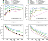 |
Fig. 13 Variations of fluxes and rotation diagrams depending on stellar parameters. Top left: same as Figure 7, but showing line fluxes for models with enhanced FUV and X-ray luminosities: 10 times (green) and 100 times (blue) the fiducial LX, and 4 times (yellow) and 40 times (pink) the fiducial LFUV. The lower-mass run (M* = 0.4 M⊙ with 10 times the fiducial LX) is also included (light green). All fluxes are computed with i = 90° and without disk obscuration. Note that the spatial integration regions and distance differ between our model and the observations (see the caption of Figure 7). Top right: same as the top-left panel, but with reduced fluxes due to disk obscuration. Bottom left: rotation diagram, same as Figure 9, but using the fluxes from the top-left panel. Bottom right: Rotation diagram using the fluxes with disk obscuration from the top-right panel. |
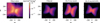 |
Fig. 14 Morphology comparison between the models and observations of Tau 042021 for the S(2) line. Left panel: frequency-integrated continuum-subtracted JWST image from Arulanantham et al. (2024). Three right panels: model S(2) images from the fiducial model (see Figure 10), the ten times X-ray model (LX ≈ 3 × 1031 erg s−1; see Section 4.3), and the test model with M* = 0.4 M⊙ and ten times the X-ray luminosity. All model images are convolved with a 2D Gaussian (FWHM ∼72au) and rotated to match the observed position angle. The circles outlined with gray dots mark the extent of our computational domain. Dashed cyan contours indicate 35%, 10%, and 3% of the peak intensity in each convolved model image; those of the fiducial model are also overplotted on the observed image, which align well with the observed morphology. The green contour in the observed image shows 35% of the peak intensity, approximating the spatial integration domain used to measure the S(2) flux in Arulanantham et al. (2024). Note that the flux integration regions differ between our models and the observations (see Figure 7 and Section 4.4.1 for details). The color scale is shared for all the panels. |
4.4.2 SY Cha
SY Cha hosts a moderately inclined transition disk (i = 51°; Orihara et al. 2023) around a K-type star with M* = 0.7 M⊙ (Manara et al. 2016; Feiden 2016; Gaia Collaboration 2021). The accretion rate has been estimated to be relatively low Ṁacc ≈ 6.6 × 10⁻¹⁰ M⊙ yr−1 but has been recently measured to be ~10−8 M⊙ yr−1, typical for accreting stars (Pittman et al. 2025). Recent JWST MIRI-MRS observations revealed extended H2 emission in the S(3)-S(7) lines, with a relatively wide semi-opening angle of θ̄open ≈ 50-60° (Schwarz et al. 2025b).
Our model (see Figure 11) broadly reproduces the morphology and surface brightness of S(3) and S(4), but the observed S(5)-S(7) emission appears more spatially extended. Conversely, the S(1) and S(2) lines show only compact emission in the observations (at least within the adopted color scales), whereas our model predicts extended conical structures when displayed on logarithmic scales.
Despite these morphological differences, the observed S(1) and S(2) fluxes measured with the radius aperture of 0.5-2" (Schwarz et al. 2025a) are consistent with those of our fiducial model (Figure 7 and Table 5) and the ten times X-ray luminosity model (Figure 13), noting that our models use d = 140 pc instead of d = 180.7 pc. A similar level of agreement is also found in the rotation diagram (bottom left panel of Figure 13).
The observationally inferred H2 mass-loss rate (3.77 ± 0.63 × 10⁻¹⁰ M⊙ yr−1) agrees well with that of the fiducial model (≈4 × 10⁻¹⁰ M⊙ yr−1) but is lower than that of the ten times X-ray case (≈2 × 10⁻⁹ M⊙ yr−1). The difference likely stems from the observational estimation method, which assumes a wind velocity of 10 km s−1 and derives the H2 column density from hot gas tracers (S(3)-S(7)). Since the hot H2 component represent only the surface layer of the H2 dominated region, the inferred massloss rate is expected to be smaller than in our model, where the most of the mass loss arises from warm gas primarily traced by S(1)-S(3) with velocities of ≲5 km s−1. In addition, if part of the observed high J emission originates from molecules excited by UV or chemical pumping, Trot can be the kinetic temperature, leading to an underestimated column density and thereby mass-loss rate. Therefore, it is unclear whether the discrepancy in the mass-loss rates is physical or merely apparent, and whether the observed low rate itself indicates a photoevaporative origin cannot be unambiguously determined within this work.
Overall, the morphological agreement is qualitative and somewhat less compelling than for Tau 042021 (Section 4.4.1), though the flux agreement is more notable. These results suggest that a photoevaporative origin also remains plausible for the H2 winds in SY Cha. However, reproducing the observed [Ne II] emission - which arises from the collimated jet - likely requires an additional MHD wind component, as in Tau 042021. Furthermore, SY Cha appears to experience markedly different irradiation conditions: its X-ray luminosity (LX ≈ 6.9 × 1029 erg s−1; Güdel et al. 2010) is about four times lower, while its FUV luminosity between 6-11 eV from ULLYSES (~9 × 1030 erg s−1; Roman-Duval et al. 2025) is roughly nine times higher than in our fiducial setup. Whether this combination of conditions can fully account for the observations remains uncertain. To properly assess the photoevaporative scenario, dedicated source-specific modeling that includes UV and chemical pumping is needed.
4.5 Caveats and future refinements
In addition to the omission of pumping in our level population calculations (Section 4.2), there are several other model limitations that should be considered in future work and when applying our results to broader systems. We outline them below.
Chemical network. To keep our simulations computationally feasible, we have adopted a reduced chemical network, which may introduce some uncertainties and limit our ability to unambiguously determine the wind origin of observed H2 winds, as discussed in Section 4.4. While the network has been validated through extensive testing (Appendix B), some effects remain unaccounted for.
For example, H2 formation via PAH catalysis may enhance the abundance of hot H2 in the H I region (Bruderer et al. 2012; Bruderer 2013). Although this depends on the poorly constrained PAH abundance, incorporating PAH-related reactions could improve model completeness, especially since PAHs have been observed in systems like Tau 042021 (Dartois et al. 2025).
Similarly, an additional uncertainty lies in the H2 formation rate on warm grains (Habart et al. 2004; Cazaux & Tielens 2004, 2010). While this process is likely ineffective within the winds in our model, where density is relatively low, it could still affect the H2 density near the base, particularly at inner radii (≲10 au).
Grain-catalyzed H2 formation is further complicated by the uncertain abundance of small grains. While we have adopted a small-dust-to-gas mass ratio of 0.0015 (assuming 85% of the dust mass has settled), recent JWST mid-infrared imaging of edge-on disks suggests that small grains may be well-mixed and more abundant in disk surfaces than previously assumed (Duchêne et al. 2024; Tazaki et al. 2025). A higher small-grain abundance would also enhance dust-gas collisional cooling. Both effects are most pronounced in high-density regions near the inner wind base, where an increased H2 abundance from enhanced grain-catalyzed formation could enable H2 to launch from smaller radii. Future studies exploring how the small-grain abundance in disk surfaces on H2 emission would be valuable for improving model completeness and jointly interpreting gas and dust observations.
Additionally, the current network includes X-ray photoionization only for H and H2 (although absorption by other species such as C and O is accounted for in the calculations of the heating rates). It may be worth exploring how including other species influences the chemical structures, especially in the context of comparing with multi-species data.
Heating and cooling processes. Not all of the X-ray energy goes into heating; some is used for ionization and excitation. This is typically encapsulated by the heating efficiency fh, which we set to fh = 0.4 for molecular gas and fh = 0.1 for atomic gas, following Xu & McCray (1991); Maloney et al. (1996). These values represent typical efficiencies for ~103 eV primary photoelectrons in neutral gas. In reality, fh depends on both photoelectron energy and the ionization degree of the ambient gas.
It can rise to f ~ 0.3-0.5 in regions with elevated electron fractions (Shull & van Steenberg 1985), such as the HI layer near the H2 dissociation front, where ye ~ 10−4−10−2 in our model. This could lead to higher temperatures and thus stronger high J emission. A more refined treatment of X-ray heating, accounting for its energy dependence and local ionization states, would improve model accuracy and strengthen comparisons with observations.
Regarding cooling, uncertainties in the elemental abundances of key coolants may also influence the resulting temperature and density structures of the H2 winds, as well as the net UV and X-ray luminosities, as discussed in Section 4.4. Accounting for such variations would be particularly important in source-specific modeling and fitting analyses.
Advection effects on level populations. The current model assumes steady-state level populations, meaning it neglects the transport of excited H2 before radiative decay. This approximation can break down in fast-moving gas, particularly under non-LTE conditions, where excited molecules may travel a characteristic distance of

The nominal value of Aul corresponds to the S(1) transition (note that, approximately,  for quadrupole lines).
In our photoevaporation model, this effect is likely minor due to the slow flow speed and the near-LTE conditions of the lowest-J lines, at least within the computational domain. It is also likely unimportant for high J lines such as S(6)-S(9), given Aul > 10−7 s−1. However, in general, this advection effect should be considered in models or observations involving emission from faster outflows.
5 Summary
While recent JWST observations have revealed the spatially resolved properties of H2 winds from PPDs (e.g., Duchêne et al. 2024; Arulanantham et al. 2024; Schwarz et al. 2025b; Pascucci et al. 2025), there are still no theoretical models to date that are directly comparable with these observations, leaving the origins of the winds uncertain. To address this gap, we have constructed the first model of photoevaporative H2 winds directly comparable with JWST data. The core questions of this study have been the morphologies and fluxes of H2 pure rotational lines, S(1)-S(9), from photoevaporative winds. Using radiation hydrodynamics simulations coupled with chemistry, we derived steady-state structures of photoevaporative H2 winds (Figure 2). We then post-processed the simulations to calculate level populations and line transfer, considering collisional (de)excitation and spontaneous decay.
In our fiducial model with M* = 1M⊙ and UV/X-ray luminosities of ~1030 erg s−1 (Table 1; Figure 1), the synthetic images exhibit the X-shaped morphology with radial extents of ≳50-300 au and semi-opening angles of θ̄open ≈ 37°-50° (Figure 5 and Table 3). The predicted line fluxes are ~10−16−10−15 erg s−1 cm−2 for the S(1)-S(5) lines, and ~10−17 erg s−1 cm−2 for the S(6)-S(9) lines, which are broadly consistent with JWST measurements (Table 2; Figure 7). However, we have likely underestimated higher J emission from extended H2 due to our neglect of UV, X-ray, or chemical pumping (Section 4.2).
We discussed how morphology and fluxes can vary with stellar parameters. Line fluxes increase with higher X-ray luminosity and lower FUV luminosity, while θ̄open widen with increasing UV and X-ray luminosities (Section 4.3; Figure 13). A lower stellar mass produces more collimated H2 winds by allowing launching from inner radii. These trends are promising but still preliminary, and more extensive modeling is needed to achieve robust conclusions.
We compared our predictions with JWST observations of Tau 042021 and SY Cha (Arulanantham et al. 2024; Pascucci et al. 2025; Schwarz et al. 2025b,a) and found remarkable agreement in morphology along with broad consistency in fluxes, especially for lower J lines (Figures 7 and 14; Table 2). For high J lines (S(5)-S(9)), again, the fluxes and spatial extents are likely underestimated (Section 4.2). In contrast to the current interpretation, these comparisons support the plausibility of a photoevaporative origin for the observed H2 winds with some remaining challenges (Section 4.4.1).
Although they are commonly used, semi-opening angles by themselves are insufficient to distinguish between MHD and photoevaporative winds unless winds are extremely collimated. Notably, PSF effects can introduce substantial biases in geometric indicators (Section 3.3 and Table 3). To better diagnose wind origins, complementary data on stellar UV/X-ray luminosities and accretion rates are essential. They would enable assessing whether the observed H2 line luminosities are energetically feasible for photoevaporation (Sections 3.2, 4.1, and 4.4). In this context, moderately inclined disks are ideal targets to explore the possibility of photoevaporative winds, as they enable both morphological and energetics analysis (see Section 4.1 for details on diagnostics of photoevaporative winds).
Overall, photoevaporation can reproduce the key features of H2 winds. However, conclusively identifying the wind origin for individual sources requires source-specific modeling, as morphology and fluxes are sensitive to stellar parameters.
Future improvements on this work include incorporating UV, X-ray, and chemical pumping in level population calculations and a broader exploration of stellar parameters. Detailed predictions from MHD models are also warranted. Together, these advances will construct a more complete framework for interpreting current and upcoming observations of disk winds.
Acknowledgements
We thank Ewine van Dishoeck, Sylvie Cabrit, and Marion Villenave for insightful discussions; Simon Bruderer for providing access to DALI; Nicole Arulanantham for sharing the JWST data of Tau 042021 and for discussions about the source; and Kamber Schwarz for helpful conversations on SY Cha; Rolf Kuiper and Alexandre Faure for their technical support with the simulations and post-processing. We are also grateful to the anonymous referee for providing the comments that have improved the quality of this paper. This research has made use of spectroscopic and collisional data from the EMAA database (https://emaa.osug.fr and https://dx.doi.org/10.17178/EMAA). EMAA is supported by the Observatoire des Sciences de l’Univers de Grenoble (OSUG). This work has made use of the Paris-Durham public shock code V1.1, distributed by the CNRS-INSU National Service “ISM Platform” at the Paris Observatory Data Center (http://ism.obspm.fr). Based on observations obtained with the NASA/ESA Hubble Space Telescope, retrieved from the Mikulski Archive for Space Telescopes (MAST) at the Space Telescope Science Institute (STScI). STScI is operated by the Association of Universities for Research in Astronomy, Inc. under NASA contract NAS 5-26555. Numerical computations were carried out on the Cray XC50 at the Center for Computational Astrophysics, National Astronomical Observatory of Japan, and on the Gattaca-2 platform at Jet Propulsion Laboratory. R.N. and G.R. acknowledge support from the European Union (ERC Starting Grant DiscEvol, project number 101039651) and from Fondazione Cariplo, grant No. 2022-1217. A.D.S. acknowledges support from the ERC grant 101019751 MOLDISK. Views and opinions expressed are, however, those of the author(s) only and do not necessarily reflect those of the European Union or the European Research Council. Neither the European Union nor the granting authority can be held responsible for them.
References
- Agra-Amboage, V., Cabrit, S., Dougados, C., et al. 2014, A&A, 564, A11 [NASA ADS] [CrossRef] [EDP Sciences] [Google Scholar]
- Alexander, R. D. 2008, MNRAS, 391, L64 [NASA ADS] [Google Scholar]
- Alexander, R., Pascucci, I., Andrews, S., Armitage, P., & Cieza, L. 2014, in Protostars and Planets VI, eds. H. Beuther, R. S. Klessen, C. P. Dullemond, & T. Henning, 475 [Google Scholar]
- Anderson, A. R., Williams, J. P., Blake, G. A., et al. 2024, ApJ, 977, 213 [NASA ADS] [CrossRef] [Google Scholar]
- Anninos, P., Zhang, Y., Abel, T., & Norman, M. L. 1997, Nature, 2, 209 [Google Scholar]
- Appenzeller, I., Oestreicher, R., & Jankovics, I. 1984, A&A, 141, 108 [Google Scholar]
- Arulanantham, N., McClure, M. K., Pontoppidan, K., et al. 2024, ApJ, 965, L13 [NASA ADS] [CrossRef] [Google Scholar]
- Bai, X.-N. 2016, ApJ, 821, 80 [Google Scholar]
- Bai, X.-N. 2017, ApJ, 845, 75 [NASA ADS] [CrossRef] [Google Scholar]
- Bajaj, N. S., Pascucci, I., Gorti, U., et al. 2024, AJ, 167, 127 [NASA ADS] [CrossRef] [Google Scholar]
- Bajaj, N. S., Pascucci, I., Beck, T. L., et al. 2025, AJ, 169, 296 [Google Scholar]
- Bakes, E. L. O., & Tielens, A. G. G. M. 1994, ApJ, 427, 822 [NASA ADS] [CrossRef] [Google Scholar]
- Ballabio, G., Alexander, R. D., & Clarke, C. J. 2020, MNRAS, 496, 2932 [NASA ADS] [CrossRef] [Google Scholar]
- Banzatti, A., Pascucci, I., Edwards, S., et al. 2019, ApJ, 870, 76 [Google Scholar]
- Banzatti, A., Abernathy, K. M., Brittain, S., et al. 2022, AJ, 163, 174 [NASA ADS] [CrossRef] [Google Scholar]
- Beck, T. L., & Bary, J. S. 2019, ApJ, 884, 159 [NASA ADS] [CrossRef] [Google Scholar]
- Beck, T. L., McGregor, P. J., Takami, M., & Pyo, T.-S. 2008, ApJ, 676, 472 [NASA ADS] [CrossRef] [Google Scholar]
- Black, J. H. 1987, Heating and Cooling of the Interstellar Gas, 134, eds. D. J. Hollenbach, & J. Thronson, A. Harley, 731 [Google Scholar]
- Black, J. H., & van Dishoeck, E. F. 1987, ApJ, 322, 412 [Google Scholar]
- Blandford, R. D., & Payne, D. G. 1982, MNRAS, 199, 883 [CrossRef] [Google Scholar]
- Brown, J. M., Pontoppidan, K. M., van Dishoeck, E. F., et al. 2013, ApJ, 770, 94 [NASA ADS] [CrossRef] [Google Scholar]
- Bruderer, S. 2013, A&A, 559, A46 [NASA ADS] [CrossRef] [EDP Sciences] [Google Scholar]
- Bruderer, S., Doty, S. D., & Benz, A. O. 2009, ApJS, 183, 179 [Google Scholar]
- Bruderer, S., van Dishoeck, E. F., Doty, S. D., & Herczeg, G. J. 2012, A&A, 541, A91 [NASA ADS] [CrossRef] [EDP Sciences] [Google Scholar]
- Cabrit, S., Ferreira, J., & Raga, A. C. 1999, A&A, 343, L61 [Google Scholar]
- Cazaux, S., & Tielens, A. G. G. M. 2002, ApJ, 575, L29 [NASA ADS] [CrossRef] [Google Scholar]
- Cazaux, S., & Tielens, A. G. G. M. 2004, ApJ, 604, 222 [NASA ADS] [CrossRef] [Google Scholar]
- Cazaux, S., & Tielens, A. G. G. M. 2010, ApJ, 715, 698 [NASA ADS] [CrossRef] [Google Scholar]
- Clarke, C. J., Gendrin, A., & Sotomayor, M. 2001, MNRAS, 328, 485 [NASA ADS] [CrossRef] [Google Scholar]
- Dalgarno, A., Yan, M., & Liu, W. 1999, ApJS, 125, 237 [NASA ADS] [CrossRef] [Google Scholar]
- Dartois, E., Noble, J. A., McClure, M. K., et al. 2025, A&A, 698, A8 [NASA ADS] [CrossRef] [EDP Sciences] [Google Scholar]
- de Valon, A., Dougados, C., Cabrit, S., et al. 2020, A&A, 634, L12 [NASA ADS] [CrossRef] [EDP Sciences] [Google Scholar]
- Draine, B. T., & Bertoldi, F. 1996, ApJ, 468, 269 [Google Scholar]
- Duchêne, G., Ménard, F., Stapelfeldt, K. R., et al. 2024, AJ, 167, 77 [CrossRef] [Google Scholar]
- Dullemond, C. P., Juhasz, A., Pohl, A., et al. 2012, RADMC-3D: A multipurpose radiative transfer tool, Astrophysics Source Code Library [record ascl:1202.015] [Google Scholar]
- Edwards, S., Cabrit, S., Strom, S. E., et al. 1987, ApJ, 321, 473 [Google Scholar]
- Ercolano, B., & Clarke, C. J. 2010, MNRAS, 402, 2735 [Google Scholar]
- Fang, M., Pascucci, I., Edwards, S., et al. 2018, ApJ, 868, 28 [NASA ADS] [CrossRef] [Google Scholar]
- Fang, M., Wang, L., Herczeg, G. J., et al. 2023, Nat. Astron., 7, 905 [Google Scholar]
- Feiden, G. A. 2016, A&A, 593, A99 [NASA ADS] [CrossRef] [EDP Sciences] [Google Scholar]
- Flores-Rivera, L., Flock, M., Kurtovic, N. T., et al. 2023, A&A, 670, A126 [NASA ADS] [CrossRef] [EDP Sciences] [Google Scholar]
- Flower, D. R., & Pineau des Forêts, G. 2003, MNRAS, 343, 390 [Google Scholar]
- Flower, D. R., Le Bourlot, J., Pineau des Forêts, G., & Roueff, E. 2000, MNRAS, 314, 753 [NASA ADS] [CrossRef] [Google Scholar]
- Flower, D. R., Pineau des Forêts, G., Hily-Blant, P., et al. 2021, MNRAS, 507, 3564 [NASA ADS] [CrossRef] [Google Scholar]
- Foucher, C., Dutrey, A., Piétu, V., et al. 2025, A&A, 704, A32 [NASA ADS] [CrossRef] [EDP Sciences] [Google Scholar]
- Gaia Collaboration (Smart, R. L., et al.) 2021, A&A, 649, A6 [EDP Sciences] [Google Scholar]
- Galli, D., & Palla, F. 1998, A&A, 335, 403 [NASA ADS] [Google Scholar]
- Gangi, M., Nisini, B., Antoniucci, S., et al. 2020, A&A, 643, A32 [NASA ADS] [CrossRef] [EDP Sciences] [Google Scholar]
- Geers, V. C., van Dishoeck, E. F., Visser, R., et al. 2007, A&A, 476, 279 [NASA ADS] [CrossRef] [EDP Sciences] [Google Scholar]
- Godard, B., Pineau des Forêts, G., Lesaffre, P., et al. 2019, A&A, 622, A100 [NASA ADS] [CrossRef] [EDP Sciences] [Google Scholar]
- González-Lezana, T., Hily-Blant, P., & Faure, A. 2021, J. Chem. Phys., 154, 054310 [CrossRef] [Google Scholar]
- Gorti, U., & Hollenbach, D. 2004, ApJ, 613, 424 [NASA ADS] [CrossRef] [Google Scholar]
- Gorti, U., Dullemond, C. P., & Hollenbach, D. 2009, ApJ, 705, 1237 [Google Scholar]
- Gredel, R., & Dalgarno, A. 1995, ApJ, 446, 852 [NASA ADS] [CrossRef] [Google Scholar]
- Gregory, S. G., Adams, F. C., & Davies, C. L. 2016, MNRAS, 457, 3836 [Google Scholar]
- Gressel, O., Turner, N. J., Nelson, R. P., & McNally, C. P. 2015, ApJ, 801, 84 [NASA ADS] [CrossRef] [Google Scholar]
- Gressel, O., Ramsey, J. P., Brinch, C., et al. 2020, arXiv e-prints [arXiv:2005.03431] [Google Scholar]
- Güdel, M., Briggs, K. R., Arzner, K., et al. 2007, A&A, 468, 353 [Google Scholar]
- Güdel, M., Lahuis, F., Briggs, K. R., et al. 2010, A&A, 519, A113 [CrossRef] [EDP Sciences] [Google Scholar]
- Güdel, M., Eibensteiner, C., Dionatos, O., et al. 2018, A&A, 620, L1 [NASA ADS] [CrossRef] [EDP Sciences] [Google Scholar]
- Habart, E., Boulanger, F., Verstraete, L., Walmsley, C. M., & Pineau des Forêts, G. 2004, A&A, 414, 531 [NASA ADS] [CrossRef] [EDP Sciences] [Google Scholar]
- Hartigan, P., Edwards, S., & Ghandour, L. 1995, ApJ, 452, 736 [Google Scholar]
- Heays, A. N., Bosman, A. D., & van Dishoeck, E. F. 2017, A&A, 602, A105 [NASA ADS] [CrossRef] [EDP Sciences] [Google Scholar]
- Hollenbach, D., & McKee, C. F. 1979, ApJS, 41, 555 [Google Scholar]
- Hollenbach, D., & McKee, C. F. 1989, ApJ, 342, 306 [Google Scholar]
- Hollenbach, D., Johnstone, D., Lizano, S., & Shu, F. 1994, ApJ, 428, 654 [NASA ADS] [CrossRef] [Google Scholar]
- Hu, X., Bae, J., Zhu, Z., & Wang, L. 2025, ApJ, 986, 161 [Google Scholar]
- Jankovics, I., Appenzeller, I., & Krautter, J. 1983, PASP, 95, 883 [Google Scholar]
- Jonkheid, B., Faas, F. G. A., van Zadelhoff, G. J., & van Dishoeck, E. F. 2004, A&A, 428, 511 [NASA ADS] [CrossRef] [EDP Sciences] [Google Scholar]
- Jonkheid, B., Kamp, I., Augereau, J. C., & van Dishoeck, E. F. 2006, A&A, 453, 163 [NASA ADS] [CrossRef] [EDP Sciences] [Google Scholar]
- Kadam, K., Vorobyov, E., Woitke, P., Basu, S., & van Terwisga, S. 2025, A&A, 695, A167 [NASA ADS] [CrossRef] [EDP Sciences] [Google Scholar]
- Kalscheur, M., France, K., Nisini, B., et al. 2025, AJ, 169, 240 [Google Scholar]
- Komaki, A., Nakatani, R., & Yoshida, N. 2021, ApJ, 910, 51 [NASA ADS] [CrossRef] [Google Scholar]
- Kuiper, R., & Klessen, R. S. 2013, A&A, 555, A7 [NASA ADS] [CrossRef] [EDP Sciences] [Google Scholar]
- Kuiper, R., Klahr, H., Dullemond, C., Kley, W., & Henning, T. 2010, A&A, 511, A81 [NASA ADS] [CrossRef] [EDP Sciences] [Google Scholar]
- Kuiper, R., Yorke, H. W., & Mignone, A. 2020, ApJS, 250, 13 [Google Scholar]
- Kunitomo, M., Suzuki, T. K., & Inutsuka, S.-i. 2020, MNRAS, 492, 3849 [CrossRef] [Google Scholar]
- Kwan, J., & Tademaru, E. 1995, ApJ, 454, 382 [NASA ADS] [CrossRef] [Google Scholar]
- Launhardt, R., Pavlyuchenkov, Y. N., Akimkin, V. V., et al. 2023, A&A, 678, A135 [NASA ADS] [CrossRef] [EDP Sciences] [Google Scholar]
- Law, D. R. E., Morrison, J., Argyriou, I., et al. 2023, AJ, 166, 45 [NASA ADS] [CrossRef] [Google Scholar]
- Lee, H.-H., Bettens, R. P. A., & Herbst, E. 1996, A&AS, 119, 111 [Google Scholar]
- Lesur, G. R. J. 2021, A&A, 650, A35 [NASA ADS] [CrossRef] [EDP Sciences] [Google Scholar]
- Lesur, G., Flock, M., Ercolano, B., et al. 2023, in Astronomical Society of the Pacific Conference Series, 534, Protostars and Planets VII, eds. S. Inutsuka, Y. Aikawa, T. Muto, K. Tomida, & M. Tamura, 465 [NASA ADS] [Google Scholar]
- Liffman, K. 2003, PASA, 20, 337 [NASA ADS] [CrossRef] [Google Scholar]
- Lique, F. 2015, MNRAS, 453, 810 [NASA ADS] [CrossRef] [Google Scholar]
- Louvet, F., Dougados, C., Cabrit, S., et al. 2018, A&A, 618, A120 [NASA ADS] [CrossRef] [EDP Sciences] [Google Scholar]
- Luhman, K. L., Mamajek, E. E., Allen, P. R., & Cruz, K. L. 2009, ApJ, 703, 399 [NASA ADS] [CrossRef] [Google Scholar]
- Maloney, P. R., Hollenbach, D. J., & Tielens, A. G. G. M. 1996, ApJ, 466, 561 [Google Scholar]
- Manara, C. F., Fedele, D., Herczeg, G. J., & Teixeira, P. S. 2016, A&A, 585, A136 [NASA ADS] [CrossRef] [EDP Sciences] [Google Scholar]
- Manara, C. F., Ansdell, M., Rosotti, G. P., et al. 2023, in Astronomical Society of the Pacific Conference Series, 534, Protostars and Planets VII, eds. S. Inutsuka, Y. Aikawa, T. Muto, K. Tomida, & M. Tamura, 539 [NASA ADS] [Google Scholar]
- McElroy, D., Walsh, C., Markwick, A. J., et al. 2013, A&A, 550, A36 [NASA ADS] [CrossRef] [EDP Sciences] [Google Scholar]
- McGinnis, P., Dougados, C., Alencar, S. H. P., Bouvier, J., & Cabrit, S. 2018, A&A, 620, A87 [NASA ADS] [CrossRef] [EDP Sciences] [Google Scholar]
- Melnikov, S., Boley, P. A., Nikonova, N. S., et al. 2023, A&A, 673, A156 [NASA ADS] [CrossRef] [EDP Sciences] [Google Scholar]
- Mignone, A., Bodo, G., Massaglia, S., et al. 2007, ApJS, 170, 228 [Google Scholar]
- Nakatani, R., Hosokawa, T., Yoshida, N., Nomura, H., & Kuiper, R. 2018a, ApJ, 857, 57 [NASA ADS] [CrossRef] [Google Scholar]
- Nakatani, R., Hosokawa, T., Yoshida, N., Nomura, H., & Kuiper, R. 2018b, ApJ, 865, 75 [Google Scholar]
- Nakatani, R., Kobayashi, H., Kuiper, R., Nomura, H., & Aikawa, Y. 2021, ApJ, 915, 90 [NASA ADS] [CrossRef] [Google Scholar]
- Nakatani, R., Turner, N. J., & Takasao, S. 2024, ApJ, 974, 281 [NASA ADS] [CrossRef] [Google Scholar]
- Nomura, H., & Millar, T. J. 2005, A&A, 438, 923 [NASA ADS] [CrossRef] [EDP Sciences] [Google Scholar]
- Nomura, H., Aikawa, Y., Tsujimoto, M., Nakagawa, Y., & Millar, T. J. 2007, ApJ, 661, 334 [NASA ADS] [CrossRef] [Google Scholar]
- Oliveira, I., Pontoppidan, K. M., Merín, B., et al. 2010, ApJ, 714, 778 [NASA ADS] [CrossRef] [Google Scholar]
- Omukai, K. 2000, ApJ, 534, 809 [NASA ADS] [CrossRef] [Google Scholar]
- Omukai, K., Hosokawa, T., & Yoshida, N. 2010, ApJ, 722, 1793 [NASA ADS] [CrossRef] [Google Scholar]
- Orihara, R., Momose, M., Muto, T., et al. 2023, PASJ, 75, 424 [CrossRef] [Google Scholar]
- Osterbrock, D. E. 1989, Astrophysics of Gaseous Nebulae and Active Galactic Nuclei (Mill Valley, CA: Univ. Science Books) [Google Scholar]
- Panoglou, D., Cabrit, S., Pineau Des Forêts, G., et al. 2012, A&A, 538, A2 [CrossRef] [EDP Sciences] [Google Scholar]
- Pascucci, I., & Sterzik, M. 2009, ApJ, 702, 724 [NASA ADS] [CrossRef] [Google Scholar]
- Pascucci, I., Sterzik, M., Alexander, R. D., et al. 2011, ApJ, 736, 13 [NASA ADS] [CrossRef] [Google Scholar]
- Pascucci, I., Banzatti, A., Gorti, U., et al. 2020, ApJ, 903, 78 [Google Scholar]
- Pascucci, I., Cabrit, S., Edwards, S., et al. 2023, in Astronomical Society of the Pacific Conference Series, 534, Protostars and Planets VII, eds. S. Inutsuka, Y. Aikawa, T. Muto, K. Tomida, & M. Tamura, 567 [NASA ADS] [Google Scholar]
- Pascucci, I., Beck, T. L., Cabrit, S., et al. 2025, Nat. Astron., 9, 81 [Google Scholar]
- Pelletier, G., & Pudritz, R. E. 1992, ApJ, 394, 117 [NASA ADS] [CrossRef] [Google Scholar]
- Perrin, M. D., Sivaramakrishnan, A., Lajoie, C.-P., et al. 2014, SPIE Conf. Ser., 9143, 91433X [NASA ADS] [Google Scholar]
- Pittman, C. V., Espaillat, C. C., Robinson, C. E., et al. 2025, ApJ, 992, 134 [Google Scholar]
- Pontoppidan, K. M., Blake, G. A., & Smette, A. 2011, ApJ, 733, 84 [Google Scholar]
- Rab, C., Weber, M., Grassi, T., et al. 2022, A&A, 668, A154 [NASA ADS] [CrossRef] [EDP Sciences] [Google Scholar]
- Rigliaco, E., Pascucci, I., Gorti, U., Edwards, S., & Hollenbach, D. 2013, ApJ, 772, 60 [NASA ADS] [CrossRef] [Google Scholar]
- Röllig, M., Abel, N. P., Bell, T., et al. 2007, A&A, 467, 187 [Google Scholar]
- Roman-Duval, J., Fischer, W. J., Fullerton, A. W., et al. 2025, ApJ, 985, 109 [Google Scholar]
- Roueff, E., Abgrall, H., Czachorowski, P., et al. 2019, A&A, 630, A58 [NASA ADS] [CrossRef] [EDP Sciences] [Google Scholar]
- Santoro, F., & Shull, J. M. 2006, ApJ, 643, 26 [NASA ADS] [CrossRef] [Google Scholar]
- Schneider, P C., Eislöffel, J., Güdel, M., et al. 2013, A&A, 557, A110 [NASA ADS] [CrossRef] [EDP Sciences] [Google Scholar]
- Schwarz, K. R., Samland, M., Olofsson, G., et al. 2025a, ApJ, 991, 232 [Google Scholar]
- Schwarz, K. R., Samland, M., Olofsson, G., et al. 2025b, ApJ, 980, 148 [Google Scholar]
- Sellek, A. D., Bajaj, N. S., Pascucci, I., et al. 2024a, AJ, 167, 223 [NASA ADS] [CrossRef] [Google Scholar]
- Sellek, A. D., Grassi, T., Picogna, G., et al. 2024b, A&A, 690, A296 [NASA ADS] [CrossRef] [EDP Sciences] [Google Scholar]
- Shoda, M., Nakatani, R., & Takasao, S. 2025, A&A, 696, L4 [NASA ADS] [CrossRef] [EDP Sciences] [Google Scholar]
- Shu, F. H., Johnstone, D., & Hollenbach, D. 1993, Icarus, 106, 92 [Google Scholar]
- Shull, J. M., & van Steenberg, M. E. 1985, ApJ, 298, 268 [NASA ADS] [CrossRef] [Google Scholar]
- Siess, L., Dufour, E., & Forestini, M. 2000, A&A, 358, 593 [Google Scholar]
- Simon, M. N., Pascucci, I., Edwards, S., et al. 2016, ApJ, 831, 169 [Google Scholar]
- Simon, M., Guilloteau, S., Beck, T. L., et al. 2019, ApJ, 884, 42 [NASA ADS] [CrossRef] [Google Scholar]
- Spitzer, L. 1978, Physical Processes in the Interstellar Medium (New York: Wiley-Interscience) [Google Scholar]
- Stapelfeldt, K. R., Duchêne, G., Perrin, M., et al. 2014, in IAU Symposium, 299, Exploring the Formation and Evolution of Planetary Systems, eds. M. Booth, B. C. Matthews, & J. R. Graham, 99 [Google Scholar]
- Suzuki, T. K., & Inutsuka, S.-i. 2009, ApJ, 691, L49 [NASA ADS] [CrossRef] [Google Scholar]
- Suzuki, T. K., Ogihara, M., Morbidelli, A., Crida, A., & Guillot, T. 2016, A&A, 596, A74 [NASA ADS] [CrossRef] [EDP Sciences] [Google Scholar]
- Tabone, B., Cabrit, S., Bianchi, E., et al. 2017, A&A, 607, L6 [NASA ADS] [CrossRef] [EDP Sciences] [Google Scholar]
- Tabone, B., Rosotti, G. P., Lodato, G., et al. 2022, MNRAS, 512, L74 [NASA ADS] [CrossRef] [Google Scholar]
- Takasao, S., Tomida, K., Iwasaki, K., & Suzuki, T. K. 2022, ApJ, 941, 73 [NASA ADS] [CrossRef] [Google Scholar]
- Tazaki, R., Ménard, F., Duchêne, G., et al. 2025, ApJ, 980, 49 [Google Scholar]
- Tielens, A. G. G. M., & Hollenbach, D. 1985, ApJ, 291, 722 [Google Scholar]
- Vicente, S., Berné, O., Tielens, A. G. G. M., et al. 2013, ApJ, 765, L38 [NASA ADS] [CrossRef] [Google Scholar]
- Villenave, M., Ménard, F., Dent, W. R. F., et al. 2020, A&A, 642, A164 [EDP Sciences] [Google Scholar]
- Wang, L., & Goodman, J. 2017, ApJ, 847, 11 [Google Scholar]
- Wang, L., Bai, X.-N., & Goodman, J. 2019, ApJ, 874, 90 [Google Scholar]
- Weber, M. L., Ercolano, B., Picogna, G., Hartmann, L., & Rodenkirch, P. J. 2020, MNRAS, 496, 223 [NASA ADS] [CrossRef] [Google Scholar]
- Weder, J., Mordasini, C., & Emsenhuber, A. 2023, A&A, 674, A165 [NASA ADS] [CrossRef] [EDP Sciences] [Google Scholar]
- Whelan, E. T., Pascucci, I., Gorti, U., et al. 2021, ApJ, 913, 43 [NASA ADS] [CrossRef] [Google Scholar]
- Wilms, J., Allen, A., & McCray, R. 2000, ApJ, 542, 914 [Google Scholar]
- Woitke, P., Kamp, I., & Thi, W. F. 2009, A&A, 501, 383 [NASA ADS] [CrossRef] [EDP Sciences] [Google Scholar]
- Woitke, P., Kamp, I., Antonellini, S., et al. 2019, PASP, 131, 064301 [NASA ADS] [CrossRef] [Google Scholar]
- Wölfer, L., Picogna, G., Ercolano, B., & van Dishoeck, E. F. 2019, MNRAS, 490, 5596 [Google Scholar]
- Xu, Y., & McCray, R. 1991, ApJ, 375, 190 [Google Scholar]
When H2 forms via chemical reactions, a portion of the binding energy, ≈4.48 eV, can go into excitation of the molecule (e.g., Hollenbach & McKee 1979).
Simon et al. (2019) report M* = 0.27 M⊙. See Section 3.4 of Duchêne et al. (2024) for a discussion on this discrepancy.
Bajaj et al. (2025) suggest the jet wiggling points to a close-in binary with a separation of ∼1.35 au and component masses of ∼0.33 M⊙ and ∼0.07 M⊙.
Appendix A Details of simulation setup
Appendix A.1 Initial disk configuration
The system is assumed to be axisymmetric and midplane symmetric, surrounding a central star with a mass of M*. The disk is initially in hydrostatic equilibrium with a vertically isothermal temperature profile, and thus the density distribution is
![Mathematical equation: \nh = n_{\rm m}(R) \exp \left[ -\frac{z^2}{2H^2} \right] , \label{eq:inidenstr}](/articles/aa/full_html/2026/02/aa56740-25/aa56740-25-eq10.png) (A.1)
(A.1)
where (R, z) are the radial distance and the vertical height in cylindrical coordinates, respectively; nH is the number density of hydrogen nuclei; nm(R) is that at the midplane (z = 0); and H is the pressure scale height defined as the ratio of the local isothermal sound speed cs to the orbital frequency  . Integrating Eq. (A.1) w.r.t. z gives the corresponding surface density profile,
 (A.2)
(A.2)
where ρm is mass density on the midplane and relates to nm in terms of mean gas mass per hydrogen nucleus, m, as ρm = mnm. The initial radial profiles of Σ is
 (A.3)
(A.3)
with R0 and Σ0 being a scale radius and reference surface density at R0. The product of Σ0 and R0 is set by the total disk mass
 (A.4)
(A.4)
with an inner and outer truncated radii, Rmin and Rmax, respectively. We use Rmin ≈ 1 au and Rmax = 40Rg ≈ 350 au in our fiducial model.
The initial temperature is assumed to be T = 100 K(R /1 au)−0∙5 but is immediately updated from the initial value according to the local thermochemical processes after the run starts. The density structure is also adjusted accordingly and reaches a steady state on a timescale of several thousand years. The results are thus insensitive to the initial condition.
Appendix A.2 Hydrodynamics
The dynamical evolution is followed by the publicly available hydrodynamics simulation code, PLUTO (Mignone et al. 2007). The code is suitably modified by implementing a variety of physics such as UV and X-ray photoheating, photochemical reactions, and multispecies chemical network (Nakatani et al. 2018a,b, 2021).
The simulation is performed in 2D spherical polar coordinates (r, θ). We follow the time evolution of gas density ρ, velocities u = (vr, vθ, vφ), total gas energy density, and chemical abundances {yi|i = H, H+, H2, ...}. The basic equations are
 (A.5)
(A.5)
 (A.6)
(A.6)
 (A.7)
(A.7)
 (A.8)
(A.8)
![Mathematical equation: \begin{split} &\frac{\partial }{\partial t}\left(\frac{1}{2} \rho v^2 + \frac{p}{\gamma-1}\right) + \nabla \cdot \left[\left(\frac{1}{2} \rho v^2 + \frac{\gamma p}{\gamma-1} \right)\vec{v}\right] \\ &\quad\quad\quad= - \rho v_r \frac{ GM_* }{r^2} +\rho \left( \Gamma -\Lambda \right), \end{split}](/articles/aa/full_html/2026/02/aa56740-25/aa56740-25-eq19.png) (A.9)
(A.9)
and
 (A.10)
Here p denotes the gas pressure; γ is specific heat ratio; Γ is the total heating rate per unit mass (specific heating rate), and Λ is the total cooling rate per unit mass (specific cooling rate); and Ri is the total reaction rate for the corresponding chemical species i. Eq. (A.8) is written in the angular momentum conserving form. For more detail regarding hydrodynamics setup, we refer the readers to Nakatani et al. (2018a,b).
Appendix B Chemistry
The chemical reactions included in our numerical simulations are listed in Table B.1. They are selected to reproduce the PDR benchmark results of Röllig et al. (2007) (Appendix B.1) while keeping the hydrodynamics simulations computationally feasible, and have also been validated through comparisons with DALI (Appendix B.2).
Reaction rates for FUV-driven photochemistry follow McElroy et al. (2013) and are expressed as k = k0χexp[-CAV], where χ is the local FUV flux normalized to the Draine field (FD ≈ 2.8 × 10⁻³ erg s−1 cm−2), k0 is the unattenuated reaction rate coefficient at χ = 1, C is a numerical constant, and AV is the visual extinction. Self-shielding is included for H2 and CO photodissociation and C I photoionization (Draine & Bertoldi 1996; Lee et al. 1996; Tielens & Hollenbach 1985). We compute AV using AV = 5∙32 × 10−22 mag cm2 × NH (DG/0.01), where NH is the hydrogen nucleus column density and DG is the small-dust-to-gas mass ratio (see Section 2.1).
The unattenuated rate coefficient k0 is calculated by integrating the product of cross-section σν and the stellar flux F*,v:

where F*,FUV is the total stellar flux in the FUV band. The crosssection data are taken from the Leiden database (Heays et al. 2017), and the integration is carried out over all frequencies up to the Lyman limit (hν ≈ 13.6 eV).
Appendix B.1 Benchmark: Plane-parallel PDR
We benchmark our chemical network against the results from various PDR codes presented in Röllig et al. (2007). We perform 1D plane-parallel PDR calculations using the parameters of the V1-V4 models of Röllig et al. (2007) and compare the resulting temperature and chemical abundance profiles with the published benchmarks. Here, we adopt a grain-catalyzed H2 formation rate coefficient of  , for consistency with the benchmarks.
Figure B.1 shows the comparison for the V4 model (high density and strong UV field). Our reduced chemical network reproduces the benchmark results with reasonable accuracy. We have confirmed a similar level of qualitative agreements for the V1-V3 models, particularly for AV ≲ 1, the regime most relevant to our study. In the low-density (V1 and V2) models, however, our network overestimates CO and underestimates CI near the CO photodissociation front, an area for potential improvement in future updates.
Appendix B.2 Benchmark: Protoplanetary disk
We also benchmark our chemical network by comparing 2D thermochemical structures with those generated by the DALI code (Bruderer et al. 2009, 2012; Bruderer 2013). For consistency, we adopt a PAH abundance set to 10% of the ISM value throughout the comparisons. To align with DALI’s setup, we disable EUV and adopt its default X-ray spectrum over 103 eV ≤ E ≤ 105 eV: LX(E) ∝ exp(-E/kTX) with the X-ray plasma temperature of TX = 7 × 10⁷K and a total luminosity of 1030 erg s−1. Other stellar parameters are taken from Table 1.
Figure B.2 shows the temperature and H2 abundance distributions for a case where the density is fixed to the initial condition of our simulation. The right panels show our reduced network reproduces the temperature and H2 abundance structures of DALI reasonably well, despite notable differences in chemical networks and computational methods. The high-temperature region (yellowish) is slightly more extended in DALI (by ~5 au), due to stronger X-ray heating in the low-column-density region, likely stemming from its use of a more detailed efficiency prescription from Dalgarno et al. (1999), compared to our simplified treatment (see Section 4.5). Overall, the agreement supports the validity of our thermochemical model.
We have performed the same comparisons while varying Ṁacc (i.e., LFUV) and bolometric luminosity, and have found a similar level of qualitative agreement. However, the match in the H2 abundance deteriorates when PAH-catalyzed H2 formation is included. This reaction enhances H2 abundances in hotter, H I-dominated region at larger radii (Bruderer et al. 2012; Bruderer 2013).
Including this reaction potentially increases high J emission while retaining lower J fluxes, which could reinforce our interpretation that the observed H2 winds are of photoevaporative origin. Nevertheless, the overall impact remains uncertain, as the formation rate is sensitive to PAH abundances, which are poorly constrained in general. Still, given the detection of PAHs in Tau 042021 (Dartois et al. 2025), it would be worthwhile to explore this effect on the flux and morphology in future work.
Additionally, DALI treats H2 pumping heating in much greater detail than the simplified approach used in the current model (Hollenbach & McKee 1979), leading to differences in the temperature structure at higher accretion rates (Ṁacc ~ 10−8 M⊙ yr−1). While this does not affect our main conclusions in the present study, it highlights an area for future improvement.
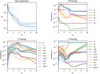 |
Fig. B.1 Comparison of temperature and chemical abundances between our thermochemical model (thick solid lines) and those from various PDR codes (thin dashed lines) from Röllig et al. (2007). |
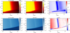 |
Fig. B.2 Comparison of gas temperature (top row) and H2 abundance (bottom row) between our model (left) and DALI (middle). Right panels: Ratio of our model to DALI. |
List of Chemical Reactions Included in Hydrodynamics Simulations
Appendix C Streamlines
Here, we present the details of our streamline analysis, following Section 3.1.
Appendix C.1 Definition of the base
A steady-state photoevaporative wind originates in a subsonic region and gradually accelerates to supersonic velocities. The flow is typically launched from a region with steep gradients in density, temperature, and heating rate, beginning with a very small - but nonzero - Mach number, as required by mass conservation (∇ · ρu = 0). Identifying the precise wind-launching point, or clearly distinguishing the wind from the underlying disk, is generally nontrivial. While one could define the wind base at the sonic surface or where the Bernoulli parameter (Etot defined in Appendix C.2) becomes positive, steady-state winds often appear to originate deeper, below these surfaces.
In this study, we define the wind base as the point where the Mach number reaches Mbase = 0.025. This value is somewhat arbitrary but chosen to ensure the wind exhibits (quasi-)steady features beyond the base (s ≥ 0, where s is the coordinate along the streamline), such as monotonically increasing velocity and Mach number, nearly conserved specific angular momentum, and consistent energy balance. As expected, the total heating rate Γ exceeds the total cooling rate Λ for s ≥ 0; otherwise, the energy input would be insufficient to sustain a wind.
For streamlines launched at larger radii (e.g., the red and cyan streamlines in Figure 3), these features are also observed for −3 au ≲ s ≲ 0 (i.e., where M < 0.025), but shifting the origin to s = −3 au does not significantly affect the profiles shown in Figures 3, 4, C.1, and C.2.
Appendix C.2 Physical properties
We provide additional details on the heating, cooling, and energetics along the representative streamlines in Figure 3. The top panels of Figure C.2 reproduce Figure 4 but include selected minor heating and cooling processes for reference.
The bottom panels show specific kinetic energy, enthalpy, gravitational potential, and centrifugal potential:

We also plot the total mechanical energy Etot = Ekin + h + Φ + El, which varies from negative to positive, along with the energy increment, ∆Etot = Etot(s) - Etot(0). This closely matches the net deposited energy

indicating the wind has reached a quasi-steady state. Also shown are the cumulative X-ray heating and H2 cooling:

for comparison.
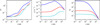 |
Fig. C.1 Same as Figure 3 but for Mach number M, X-ray ionization rate coefficient, and G0 along the three streamlines. |
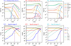 |
Fig. C.2 (top) Specific rates of major heating and cooling processes along the three streamlines in Figure 3, shown from left to right for the blue, red, and cyan streamlines. Labels indicate: EUV photoionization heating (“EUV”); FUV grain photoelectric heating (“Photoele”); X-ray photoionization heating (“X-ray”); H2 photodissociation heating (“Photodis”); H2 pumping followed by collisional deexcitation (“Pump”); chemical heating from dust-catalyzed H2 formation (“chem”); radiative recombination cooling (“rec”); line cooling from OI, H2, and CO; and adiabatic cooling (“adi”). (bottom) Specific energy components along the same streamlines. Blue, red, black, and orange lines show the poloidal kinetic energy, enthalpy, gravitational potential (absolute value), and centrifugal potential, respectively. The purple line indicates total mechanical energy Etot, which varies from negative to positive. Dashed pink line shows the total energy increment, ∆Etot = Etot(s) − Etot(0), which closely overlaps the dashed cyan line showing the total net deposited energy from heating and cooling. Thin green and dashed yellow lines represent energy input from X-ray heating and losses via H2 cooling. On the left panel, the green, cyan, and pink lines nearly coincide. |
Appendix D Mass-loss rates
Here, we evaluate the cumulative mass-loss rates Ṁ(R) and surface mass-loss rates Σ̇ from our fiducial simulation.
The cumulative mass-loss rate Ṁ(R) represents the total mass lost through gas launched from < R. To compute it, we first calculate the total mass flux through the outer computational boundary as a function of θ:

We then trace a streamline back from the outer boundary (rmax, θ) to identify the corresponding wind-launching radius R, defined following the method in Appendix C.1. The cumulative massloss rate Ṁ(R) is then given by Ṁout(θ). This estimate excludes contributions from gas that does not satisfy the unbound condition before reaching the outer boundary along the streamline: Etot > 0. The corresponding surface mass-loss rates is defined as

We similarly compute the cumulative and surface mass-loss rates for H2.
These results are shown in Figure D.1. Note that the total mass-loss rates (black lines) include helium contributions. Therefore, H2 is responsible for almost all the surface mass loss of hydrogen-bearing species at ≳40 au.
The sharp cutoff in Ṁ and Σ̇ at R ~ 220 au reflects the computational boundary, beyond which launched gas do not meet the unbound condition. This is a numerical artifact; a larger domain would likely extend the wind-launching region farther out.
Toward the inner disk, the total Σ̇ increases with decreasing radius. This again highlights a limitation of our computational domain, which does not resolve the critical radius (~1 au), where Σ̇ is expected to plateau and sharply drop inward.
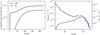 |
Fig. D.1 Cumulative (left) and surface (right) mass-loss rates, with black and blue lines indicating the total and H2 mass-loss contributions, respectively. Note that the total mass-loss rates include the contributions from helium-bearing species. |
All Tables
Comparison of model fluxes for different inclinations with and without disk obscuration.
All Figures
|
Fig. 1 Stellar spectrum adopted in our fiducial model. The vertical dashed lines mark the lower energy limits of the FUV and EUV bands. The lower limit of the X-ray band is 100 eV. (See also Table 1 for the integrated luminosities.) The thin green line shows the photospheric emission, which overlaps with the blue line below 6 eV, for reference. |
| In the text | |
|
Fig. 2 Snapshot of H2 density (top), gas temperature (second), H2 abundance (third), and poloidal velocity (bottom). Cyan contours indicate isosurfaces for each quantity: nH2 = 10, 102, 103, 104, 105, 106, 107cm−3; T = 200, 500, 1000, 2000, 3000, 5000K; yH2 = 10−4,10−3,10−2,10−1; and vp = 1,2,5,10,20,30km s−1. In all panels, the white and green dashed contours denote the H2 dissociation front (yH2 = 0.25) and the isothermal sonic surface, respectively. White arrows indicate the velocity field (direction only, not its magnitude) and are omitted where T < 100K. In the H2 abundance map, the dotted gray contour marks the HI ionization front (yHII = 0.5). |
| In the text | |
|
Fig. 3 Physical properties along streamlines. (a) H2 abundance map (same as Figure 2) with selected streamlines shown in gray. Three representative streamlines are marked in blue, red, and cyan. (b-f) Profiles of cylindrical radius, densities, temperature, poloidal velocity, and H2 abundance along the three streamlines, using consistent color coding. The horizontal axis indicates the distance along each streamline, with s = 0 defined at the base. In panel c, solid and dashed lines show H2 and hydrogen nucleus densities, respectively. |
| In the text | |
|
Fig. 4 Specific rates of major heating and cooling processes along the blue, red, and cyan streamlines in Figure 3, shown from left to right. Labels indicate: EUV photoionization heating (“EUV”); X-ray photoionization heating (“X-ray”); line cooling from O I, H2, and CO; and adiabatic cooling (“adi”). (See Figure C.2 in Appendix for the heating and cooling rates of other processes.) |
| In the text | |
|
Fig. 5 Intrinsic morphologies of the H2 pure rotational lines (S(1)-S(9)) for a disk viewed edge-on (i = 90°) without disk obscuration. The colors indicate the frequency-integrated intensities, with individual color bars scaled independently in each panel, Right ascension and declination offsets are shown assuming a source distance of d = 140 pc. |
| In the text | |
|
Fig. 6 Comparison of emission morphologies between the intrinsic and Gaussian-convolved S(2) images. Top panel: original image from Figure 5. Bottom panel: same image convolved with a Gaussian kernel of FWHM ∼72 au. |
| In the text | |
|
Fig. 7 Integrated fluxes of the S(1)-S(9) lines for the model with i = 90° without disk obscuration and assuming d = 140 pc (black dots). For reference, green crosses indicate the fluxes calculated under the assumptions of LTE and optically thin emission. Observed fluxes for SY Cha (blue; d = 180.7 pc) and Tau 042021 (red; d ~ 140 pc) are also shown for comparison. For SY Cha, we adopted the fluxes measured with a radius aperture of 0.5-2″. Since the spatial integration regions differ between our model and the observations of Tau 042021, and the SY Cha fluxes are not scaled by distance, care should be taken when making direct comparisons (see also Sections 4.4.1 and 4.4.2 and Figure 14). Open circles correspond to the model fluxes with i = 90° but including disk obscuration (Section 3.7; Table 5). |
| In the text | |
|
Fig. 8 Phase-space scatter plots of the normalized local integrated luminosity LJ/LJ,max for each H2 line. Each point corresponds to a computational cell in the simulation, with point size scaled by LJ/LJ,max to reduce overlap and emphasize more emissive regions. The reddish areas highlight the densities and temperatures ranges that most strongly contribute to the total emission. Solid black lines mark approximate contours of poloidal wind velocity (vp = 1, 3, and 5 km s−1), and the green contour indicates the isothermal sonic surface. Dashed blue lines represent the best-fit rotational temperatures (Table 4). |
| In the text | |
|
Fig. 9 Rotation diagram of the H2 lines. Black dots show the model results from non-LTE calculations with line transfer using RADMC-3D. The solid and dashed black lines are a two-component fit to the lower J lines S(1)-S(3) and the higher J lines S(4)-S(9), respectively. Green crosses indicate the values assuming LTE and optically thin emission -i.e., the maximum emission possible within our model setup. For reference, observational data for SY Cha are shown with a blue line (Schwarz et al. 2025a). Since the emitting area is not specified in Arulanantham et al. (2024), the data for Tau 042021 are omitted to avoid introducing additional uncertainties. |
| In the text | |
|
Fig. 10 Same as Figure 5, but including dust extinction within the disk. The panels show continuum-subtracted images. |
| In the text | |
|
Fig. 11 Same as Figures 5 and 10 but for an inclination of i = 60° including dust extinction within the disk. |
| In the text | |
|
Fig. 12 Velocity profiles of selected lines viewed at inclinations of i = 0° (purple), 30° (cyan), 45° (light green), 60° (yellow), and 90° (red). For i < 90°, the profiles were computed excluding emission from the far side of the disk, isolating the contribution from the near-side surface. |
| In the text | |
|
Fig. 13 Variations of fluxes and rotation diagrams depending on stellar parameters. Top left: same as Figure 7, but showing line fluxes for models with enhanced FUV and X-ray luminosities: 10 times (green) and 100 times (blue) the fiducial LX, and 4 times (yellow) and 40 times (pink) the fiducial LFUV. The lower-mass run (M* = 0.4 M⊙ with 10 times the fiducial LX) is also included (light green). All fluxes are computed with i = 90° and without disk obscuration. Note that the spatial integration regions and distance differ between our model and the observations (see the caption of Figure 7). Top right: same as the top-left panel, but with reduced fluxes due to disk obscuration. Bottom left: rotation diagram, same as Figure 9, but using the fluxes from the top-left panel. Bottom right: Rotation diagram using the fluxes with disk obscuration from the top-right panel. |
| In the text | |
|
Fig. 14 Morphology comparison between the models and observations of Tau 042021 for the S(2) line. Left panel: frequency-integrated continuum-subtracted JWST image from Arulanantham et al. (2024). Three right panels: model S(2) images from the fiducial model (see Figure 10), the ten times X-ray model (LX ≈ 3 × 1031 erg s−1; see Section 4.3), and the test model with M* = 0.4 M⊙ and ten times the X-ray luminosity. All model images are convolved with a 2D Gaussian (FWHM ∼72au) and rotated to match the observed position angle. The circles outlined with gray dots mark the extent of our computational domain. Dashed cyan contours indicate 35%, 10%, and 3% of the peak intensity in each convolved model image; those of the fiducial model are also overplotted on the observed image, which align well with the observed morphology. The green contour in the observed image shows 35% of the peak intensity, approximating the spatial integration domain used to measure the S(2) flux in Arulanantham et al. (2024). Note that the flux integration regions differ between our models and the observations (see Figure 7 and Section 4.4.1 for details). The color scale is shared for all the panels. |
| In the text | |
|
Fig. B.1 Comparison of temperature and chemical abundances between our thermochemical model (thick solid lines) and those from various PDR codes (thin dashed lines) from Röllig et al. (2007). |
| In the text | |
|
Fig. B.2 Comparison of gas temperature (top row) and H2 abundance (bottom row) between our model (left) and DALI (middle). Right panels: Ratio of our model to DALI. |
| In the text | |
|
Fig. C.1 Same as Figure 3 but for Mach number M, X-ray ionization rate coefficient, and G0 along the three streamlines. |
| In the text | |
|
Fig. C.2 (top) Specific rates of major heating and cooling processes along the three streamlines in Figure 3, shown from left to right for the blue, red, and cyan streamlines. Labels indicate: EUV photoionization heating (“EUV”); FUV grain photoelectric heating (“Photoele”); X-ray photoionization heating (“X-ray”); H2 photodissociation heating (“Photodis”); H2 pumping followed by collisional deexcitation (“Pump”); chemical heating from dust-catalyzed H2 formation (“chem”); radiative recombination cooling (“rec”); line cooling from OI, H2, and CO; and adiabatic cooling (“adi”). (bottom) Specific energy components along the same streamlines. Blue, red, black, and orange lines show the poloidal kinetic energy, enthalpy, gravitational potential (absolute value), and centrifugal potential, respectively. The purple line indicates total mechanical energy Etot, which varies from negative to positive. Dashed pink line shows the total energy increment, ∆Etot = Etot(s) − Etot(0), which closely overlaps the dashed cyan line showing the total net deposited energy from heating and cooling. Thin green and dashed yellow lines represent energy input from X-ray heating and losses via H2 cooling. On the left panel, the green, cyan, and pink lines nearly coincide. |
| In the text | |
|
Fig. D.1 Cumulative (left) and surface (right) mass-loss rates, with black and blue lines indicating the total and H2 mass-loss contributions, respectively. Note that the total mass-loss rates include the contributions from helium-bearing species. |
| In the text | |
Current usage metrics show cumulative count of Article Views (full-text article views including HTML views, PDF and ePub downloads, according to the available data) and Abstracts Views on Vision4Press platform.
Data correspond to usage on the plateform after 2015. The current usage metrics is available 48-96 hours after online publication and is updated daily on week days.
Initial download of the metrics may take a while.