| Issue |
A&A
Volume 706, February 2026
|
|
|---|---|---|
| Article Number | A370 | |
| Number of page(s) | 20 | |
| Section | Galactic structure, stellar clusters and populations | |
| DOI | https://doi.org/10.1051/0004-6361/202557920 | |
| Published online | 25 February 2026 | |
The stellar initial mass function of nearby young moving groups
1
Departamento de Astronomía, Facultad de Ciencias, Universidad de la República,
Iguá 4225,
Montevideo,
CP
11400,
Uruguay
2
Steward Observatory and Department of Astronomy, University of Arizona,
933 N. Cherry Avenue,
Tucson,
AZ
85721,
USA
3
American Museum of Natural History,
200 Central Park W,
New York,
NY
10024,
USA
4
Planétarium de Montréal,
Montréal,
Québec,
Canada
5
Trottier Institute for Research on Exoplanets, Université de Montréal, Département de Physique,
Montréal,
Québec,
Canada
6
Universidad Nacional Autónoma de México, Instituto de Astronomía,
AP 106,
Ensenada
22800,
BC,
Mexico
★ Corresponding author: This email address is being protected from spambots. You need JavaScript enabled to view it.
Received:
30
October
2025
Accepted:
27
December
2025
Abstract
Context. The solar neighbourhood is populated by nearby (<200 pc), young (<100 Myr) moving groups (NYMGs) of stars, whose origins are still a matter of debate. One plausible explanation is that they are remnants of individual stellar clusters and associations that are currently dispersing throughout the galactic disc.
Aims. We aim to derive the initial mass function (IMF) of a large sample of NYMGs.
Methods. We developed and applied an algorithm that uses photometric and astrometric data from Gaia DR3 to detect NYMGs as over-densities in a kinematic space, whose members distribute along young isochrones. We inferred individual masses from the photometry of both the detected and the previously known candidates. We estimated the IMFs for 33 groups, 30 of them for the first time, in an average mass range 0.1 < m/M⊙ < 5, with some groups going as low as 0.02 M⊙ and as high as 10 M⊙. We parameterised these IMFs using a log-normal for m < 1 M⊙ and a power-law for m > 1 M⊙.
Results. We detected 4166 source candidate members of 44 known groups, including 2545 new candidates. We recovered 44-54% of the literature candidates and estimated a contamination rate from old field stars of 16-24%. The candidates of the detected groups distribute along young isochrones, which suggests that they are potential members of NYMGs. Parameterisations of both the average of the 3 3 IMFs based on our detections (mc = 0.25 ± 0.17 M⊙, σc = 0.45 ± 0.17, and α = −2.26 ± 0.09) and the one based on the known candidates from the literature (mc = 0.22 ± 0.14 M⊙, σc = 0.45 ± 0.17, and α = −2.45 ± 0.06) are in agreement with the IMF parameterisation of the solar neighbourhood and young stellar associations.
Conclusions. Our parameterisation of the average IMF, together with the distribution of the detected group members along young isochrones offer strong evidence suggesting that the NYMGs are remnants of individual stellar associations and clusters. We confirm that there are no systematic biases in our detection and in the literature in the range of 0.1 < m/M⊙ < 10.
Key words: open clusters and associations: general / solar neighborhood / Galaxy: structure
© The Authors 2026
 Open Access article, published by EDP Sciences, under the terms of the Creative Commons Attribution License (https://creativecommons.org/licenses/by/4.0), which permits unrestricted use, distribution, and reproduction in any medium, provided the original work is properly cited.
This article is published in open access under the Subscribe to Open model. This email address is being protected from spambots. You need JavaScript enabled to view it. to support open access publication.
1 Introduction
The initial mass function (IMF) is the distribution of stellar and sub-stellar masses resulting from a single star formation event (e.g. Hopkins 2018). Despite extensive research since its first observational determination (Salpeter 1955), the central question about its universality, namely, the question of whether the IMF of all stellar populations originates from the same distribution, remains a subject of intense research. Reviews from Bastian et al. (2010), Offner et al. (2014), and Hopkins (2018), show that while the IMF in the mass range 0.1 < M/M⊙ < 10 is roughly consistent across different nearby populations in the Milky Way, there are exceptions, such as Upper Sco (Slesnick et al. 2008). The large uncertainties involved prevent the IMF from being adequately constrained, particularly in the sub-stellar mass domain. Furthermore, Dib (2023) found a correlation between the slope of the high-mass end of the IMF and the surface density of young clusters, suggesting a dependence of the massive star formation on the environment. Additionally, the extent to which observational and methodological biases have influenced our understanding of the IMF remains unclear (Hopkins 2018). Thus, more statistically robust observational studies of the IMF are needed to explore its universality.
Numerous stellar comoving groups have been found in the solar neighbourhood (e.g. Gagné & Faherty 2018) with ages varying from a few Myr to a Gyr. Among these groups are the nearby young moving groups (NYMGs), which we consider here as those younger than 100 Myr at distances shorter than 200 pc. Currently, 68 groups meet these characteristics according to the Montreal Open Clusters and Associations (MOCA; Gagné 2024) database, with a total of a few hundred known stellar and sub-stellar members extensively studied (e.g. Gagné et al. 2021 and references therein). The most widely accepted hypothesis regarding the origin of these groups suggests that they are remnants of stellar associations and disrupted clusters that are now being scattered across the galactic disc (Gagné et al. 2021) as a consequence of their stars having formed gravitationally unbound within their parental molecular cloud, as expected from most stellar populations (Lada & Lada 2003). Based on this idea, several efforts have been made to integrate the orbits of young comoving groups located as far as 1 kpc (e.g. Fernández et al. 2008; Quillen et al. 2020; Swiggum et al. 2024). Although these works present different spatial origin to these groups, they all suggest they formed from giant molecular clouds structures within or related to the passage of spiral arms.
The young ages and proximity of NYMGs make them natural targets for determining the IMF because they should have lost only their most massive stars as a consequence of stellar evolution, and their closeness allows for both the observation of the least massive members and the detection of some binary systems. However, there are some significant challenges in identifying the members of each NYMG: (i) their proximity make the NYMGs project onto extensive regions of the sky; (ii) most NYMGs are loose associations with a small number of members, producing subtle over-densities in phase-space; and (iii) if these groups are indeed scattering through the galactic disc, some members may have completely lost their kinematic memory, making it impossible to determine their membership.
The IMF of NYMGs is relevant in the description of the solar neighbourhood. Despite progress in identifying and characterising NYMGs and their members, there are, to our knowledge, only three studies of the IMF of NYMGs. The first corresponds to Gagné et al. (2017), who focused on the TW-Hya association. They inferred the IMF from 55 candidate members (0.01 < m/M⊙ < 2), finding a log-normal distribution with a characteristic mass,  , consistent with previous results for the solar neighbourhood (mc = 0.20 ± 0.05 M⊙; Chabrier 2005), and a width of
  dex, which they claim is significantly larger than the 0.3-0.55 dex usually found in young associations. However, the authors stress that their results could be biased by an unknown observational or physical effect, especially in the low-mass regime, which could explain the large σ. The second study corresponds to Gagné et al. (2018), who inferred the IMF of the Volans-Carina group in the mass range 0.15 < m/M⊙ < 3. In this work, they were able to identify 58 candidate members with parallaxes from Gaia Data Release 2, from which they inferred their mass distribution. They concluded that the mass distribution found is well described by a fiducial log-normal IMF with mc = 0.25 M⊙ and σc = 0.5 in the range m > 0.2 M⊙, suggesting their census of this group is almost complete. Finally, Kraus et al. (2014) inferred the IMF of Tucana-Horologium. They found that when compared to the typical solar neighbourhood IMF (Chabrier 2005; Salpeter 1955), there appear to be signs of incompleteness in the mass range 0.2 < m/M⊙ < 0.7. However, they claim that it is not clear if this is indeed the product of a true incompleteness in the data or the result of an error in the stellar models they used that could have pulled stars of spectral types M0-M1 to spectral types K7.5.
In this work, we present the development and application of a method to identify members of NYMGs and infer their IMFs in the mass range 0.02 < m/M⊙ < 10 based on photometric and astrometric data from Gaia Data Release 3 (Gaia Collaboration 2023) and the DBSCAN algorithm (Ester et al. 1996). We only focus on 44 of the 68 known NYMGs from the literature, which we were able to detect. In Sect. 2, we describe how we selected and completed the sample of all GDR3 sources within 200 pc from the Sun and the compilation of known NYMG members and bona fide candidates from the literature. In Sect. 3, we explain the detection algorithm to find NYMGs and the significance of the results. In Sect. 4, we apply Bayesian inference to estimate masses from photometry and parallaxes and present the resulting IMFs characterised in terms of their purity, completeness, and parameterisation. Finally, in Sect. 5, we summarise our results and present our conclusions.
2 The samples
We conducted our search using the GDR3 catalog, which offers the best combination to date of spatial and photometric completeness, as well as precision in photometric and astrometric data for the solar neighbourhood. As a validation sample, we compiled a list of known confirmed members and bona fide candidates of NYMGs from MOCA.
2.1 The Gaia sample in the solar neighbourhood
Our starting sample corresponds to the 5 244 458 GDR3 sources with parallaxes of ϖ ≥ 5 mas, after applying the zero-point correction for w provided by the gaiadr3_zeropoint Python package based on Lindegren et al. (2021). The resulting sample corresponds to distances d ≤ 200 pc, if we assume d = 1/ϖ. As shown in Appendix A, distances estimated in this way show good agreement (with different distance estimates for less than ~5% of the sample, almost all fainter than G = 17 mag) with the photo-geometric distances estimated by Bailer-Jones et al. (2021) if we impose a threshold of < 0.1 on parallax fractional error (mϖ/ϖ). Additionally, we estimated that only ~1.3% of the stars that truly belong to the solar neighbourhood are discarded with this method. Only 43% of the starting sample sources fulfill the condition mϖ/ϖ < 0.1, which corresponds to almost all sources from GDR3 with photo-geometric distances smaller than 200 pc.
We defined two subsets from the starting sample of GDR3 sources with ϖ ≥ 5 mas: S and SNYMG. The first sample is defined to select all the solar neighbourhood sources with precise magnitudes and parallaxes that could be potential NYMG members. The sample SNYMG is the result of applying additional photometric and astrometric cuts to the sources from S. The sample, S, was obtained by applying the following conditions to the GDR3 sources with ϖ ≥ 5 mas:
Precise parallaxes: We discarded sources with mϖ/ϖ > 0.1 to ensure that 1/ϖ is a good estimate of d.
Main sequence (MS) and pre-main sequence (PMS) stellar and substellar objects: We discarded all sources outside the MS and PMS locus in the MG vs BP - RP colour-absolute magnitude diagram (CMD), as shown in Fig. 1.
Precise G magnitudes: We discarded all sources with signal-to-noise ratio (S/N) in the G passband of log10(FG/σFG) < 2.2, where FG and σFG are the flux and the corresponding uncertainty, respectively. Most of the discarded sources appear in a non-physical position on the colour magnitude diagram (CMD) for stars (overdensity around BP - RP = 2 mag and MG = 14 mag in Fig. 1), probably due to unreliable parallaxes as a result of crowding for being near the galactic plane (Gaia Collaboration 2021b). Additionally, many of these sources show proper motions very close to zero, suggesting they could also be extragalactic sources.
Coherent tangential velocities: we discarded sources with tangential velocities
![Mathematical equation: $[v_{\alpha_{LSR}}^2+v_{\delta_{LSR}}^2]^{1/2} > 20$](/articles/aa/full_html/2026/02/aa57920-25/aa57920-25-eq3.png) km s−1, where vαLSR and vδLSR are the components of the tangential velocity in the local standard of rest (LSR) computed using d, the equatorial coordinates (α,δ), and the proper motions (μα,μδ). The 20 km s−1 corresponds to the maximum value for the NYMG members, as shown in Appendix D.
km s−1, where vαLSR and vδLSR are the components of the tangential velocity in the local standard of rest (LSR) computed using d, the equatorial coordinates (α,δ), and the proper motions (μα,μδ). The 20 km s−1 corresponds to the maximum value for the NYMG members, as shown in Appendix D.
Although the conditions on σϖ/ϖ and the photometric S/N might primarily exclude some faint objects and, as a result, affect the lower end of the IMF, in Appendix A.1, we estimate that this corresponds to only ~1.3% of the objects in the sample, S. The sample, SNYMG, was obtained by applying the following quality conditions to the S sample:
Uncontaminated photometry: we discarded sources whose photometry is affected by contamination from other sources and other effects by applying the condition suggested by Gaia Collaboration (2021a): log10(phot_bp_ rp_excess_factor) ≤ 0.001 + 0.039(GBP - GRP) or 0.012 + 0.039(GBP - GRP) ≤ log10(phot_bp_rp_excess_factor), where GBP and GRP are magnitudes in the Gaia passbands and phot_bp_rp_excess_factor = (FBP + FRP)/FG is the flux excess.
Reliable astrometry: we discarded sources with bad astrometry, often caused by multiplicity. To do so, we followed the prescription from Fabricius et al. (2021) and applied the condition ruwe ≥ 1.4, where ruwe is the re-normalised unit weighted error (Lindegren 2018). This condition affects the entire sample and removes potential multiple systems that will not be included in the IMFs. We show in Sect. 2.2 how we corrected the sample for these missing sources.
Figure 1 shows the CMD distribution of the starting sample as well as the S and SNYMG samples together with the corresponding number of sources. The isochrones in the figure were obtained from a combination of three sets of different stellar and substellar evolutionary models: (1) the ATMO 2020 models by Phillips et al. (2020) for masses 0.01 ≤ M/M⊙ ≤ 0.015 and ages younger than 20 Myr, as well as masses 0.01 ≤ M/M⊙ ≤ 0.03 and ages older than 20 Myr, following the conclusions of Sect. 5.5 from Phillips et al. (2020); (2) the Baraffe et al. (2015) models for ages and masses greater than the previous limits and up to 0.75 M⊙ ; and (3) the Marigo et al. (2017) models for masses 0.75 < M/M⊙ < 10.
Figure 1 also shows a reference extinction vector for an M4 dwarf star with AV = 0.22 mag, which corresponds to the average extinction for the known NYMG candidate members (Sect. 2.3), according to the 3D extinction maps from Gontcharov (2017). As Gaia’s photometric BP, RP, and G bands are very wide (effective widths ≳ 300 nm), the colour dependence on extinction laws in those bands cannot be ignored, as demonstrated in Appendix A from Ramos et al. (2020)1, who shows that Gaia’s extinction law in the G band drastically decreases with BP-RP from kG ~ 1 for BP-RP~0 to kG ~ 0.55 mag for BP-RP~4 mag. As the expressions E(RP -J)/E(J - H) ≃ 2.4, E(G - RP)/E(J - H) ≃ 0.6, and E(BP -RP)/E(J - H) ≃ 3 were estimated by Luhman (2021) for the overall associations of Upper Sco and Ophiuchus, they can be used to estimate an average extinction across spectral types. Using these equations together with the values kJ = 0.282, kH = 0.175 and kκ = 0.112 from Rieke & Lebofsky (1985), we were able to estimate that on average for an M4 dwarf in an NYMG ABP - ARP ≈ 0.11 mag and AG ≈ 0.13 mag. Since the value of AG is very small (and should be even smaller for fainter stars because of the previously mentioned colour dependence) only the faintest stars can be dimmed beyond the completeness photometric limit (G ~ 17 mag) as a consequence of extinction. The reddening component, ABP - ARP, of the extinction vector, however, is non-negligible and must be taken into account in the inference of mass based on photometry. Finally, we note that SNYMG may lack some of the brightest stars of the solar neighbourhood since sources with G < 3 mag are not included in Gaia (Gaia Collaboration 2021b). Although this may affect the high-mass end of the IMF, if these groups contain low numbers of members as suggested by the literature (see Sect. 2.3) and assuming that their IMF follows some power-law like any other stellar population, then they should contain very low numbers of high-mass stars, which we would expect to be comparable with Poisson’s noise. This means that although we might be missing some very massive stars, their absence should not significantly affect the statistical behaviour of the measured IMFs.
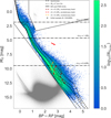 |
Fig. 1 CMD of the starting sample (grey points) and the SNYMG sample (coloured scale indicating the density of points). The solid lines indicate the limits of the MS and PMS locus, the black dashed curves show the isochrones from Phillips et al. (2020), Baraffe et al. (2015), and Marigo et al. (2017) stellar evolutionary models for 10 Myr, 30 Myr, 100 Myr, and 1 Gyr. The horizontal black dash-dotted lines indicate the MG values corresponding to the turn-on (see Sect. 3.5) for the labelled masses. The red, orange, and blue dashed lines indicate the 0.1, 0.2, and 0.3 Μ⊙ evolutionary tracks, respectively. The red arrow indicates twice the extinction vector for an M4 dwarf star with AV = 0.22 mag. |
2.2 Towards a complete Gaia sample of the solar neighbourhood
It is expected that SNYMG will suffer from some level of incompleteness due to the combination of the intrinsic biases of the GDR3 survey and potential biases introduced by the conditions we used to build it. This incompleteness could compromise the correct identification of some of the groups or some of their substructures and ultimately affect our measurement of their IMFs. We used the GaiaUnlimited selection functions (GSFs; Castro-Ginard et al. 2023) Python library and the prescription from Appendix B to estimate the real completeness of SNYMG, which we define as the number of stars that we are effectively studying, divided by the real number of stars that we wish to study.
The GSFs give us the tools to compute the general selection function of GDR3. This corresponds to a continuous map, F(q), defined in a four-dimensional (4D) space of observables, q = (α,δ, G - RP, G), that returns, for a given q, the probability F(q) = Pq(GDR3) that a source with q ∈ ∆q = (q - dq, q + dq) has made it into GDR3. As explained by Rix et al. (2021), for each q, F(q) is a dimensionless probability with values between 0 and 1, which is why F(q) is not a probability distribution over all q. The GSFs also contain tools to directly estimate the selection function of a sub-sample C based on some arbitrary conditions applied to the GDR3 catalogue. In other words, it allows us to estimate the probability FC(q) = Pq(C|GDR3) that a source with q ∈ (q - dq, q + dq) belongs to C, knowing that the source is in GDR3. Then, from Appendix B, the fraction of real completeness fq for q ∈ (q - dq, q + dq) can be estimated as
 (1)
(1)
where Sreal stands for the real sample of MS and PMS stars in the solar neighbourhood (i.e. the sample that we wish to study. The term Pq(GDR3) represents the probability that a star with observables q is in GDR3, while the term  approximates the probability that this star ends up in the final sample SNYMG, assuming that it belongs to ancillary sample S defined in Sect. 2.1. If these two probabilities are independent, their product should approximate the value of fq.
As discussed in Sect. 3.2, our work focuses on the fivedimensional (5D) kinematic space (X,Y,Z,vαLSR,vδLSR) that we call the restricted phase-space (RPS) and the CMD (BP-RP,MG). The RPS is defined as the union of the galactic Cartesian positions (X,Y,Z) and the equatorial tangential velocities in the LSR (vαLSR,vδLSR). We only need to increase the completeness of SNYMG in the RPS and the CMD. To do so, we first divide SNYMG into ∆q bins of 1 mag in G, 0.1 mag in G - RP and a HEALPix level of 4 for (α, δ). Then, we computed fq for each ∆q using Eq. (1), counted the number of stars NΔq in ∆q, and stochastically sampled NΔq/fq - NδQ stars from a model of the 7D kinematic and photometric distribution (X,Y,Z,vαLSR,vδLSR,G,BP-RP). Assuming that the dependence between the RPS and CMD distribution is negligible, we sampled these two spaces separately, using the full SNYMG for the RPS and only the sources from this sample within ∆q to model the CMD. We used a kernel density estimator (KDE) with a Gaussian kernel to model the RPS distribution. The KDE is built by multiplying all the velocities by 10 pc km−1 s, so the scale is the same for positions and velocities. In this rescaled space, we used a bandwidth equal to the 90th percentile of the kinematic errors of the SNYMG sample in that scaled RPS, which is ≈9.72 pc. For the CMD, we modelled the SNYMG sources in ∆q by sampling the cumulative distributions of MG within BP-RP bins of 0.1 mag across the entire BP-RP range of −0.5 to 5 mag.
The resulting catalogue Sc includes the SNYMG sample plus NΔq/fq - NΔq synthetic sources. We created ten realisations of Sc to achieve more statistically robust results. As expected, the number of added synthetic sources increases with G and G - RP because the completeness decreases for fainter sources.
As explained in Appendix B, Eq. (1) and the GSFs do not account for potential incompleteness in the S sample due to the quality conditions log10(S/N)>2.2 and σϖ/ϖ < 0.1. However, as explained in Appendix A, we estimated that these conditions only excluded ~7000 objects (~1.3% of final sample) that would have been part of S and that could belong to the solar neighbourhood, according to Bailer-Jones et al. (2021), which would have corresponded to only ~ 1% of S.
2.3 The catalogue of known members and candidates
In this study, we consider a source is a candidate member of a specific known NYMG if its photometry and kinematics from GDR3 are consistent with those of previously known members of the NYMG. We used the MOCA database (Gagné 2024) to compile most of the objects reported in the literature as members of the NYMGs following the prescription from Appendix C. This catalogue includes relevant information from most, if not all of the known groups in the literature. We only kept in the resulting sample candidate members from MOCA with a membership probability estimated by BANYAN in April 2025 p > 0.95.
The resulting sample consists of a total of 5926 sources distributed between 68 different NYMGs. In this work, and as discussed in Sect. 3.4, we were able to re-detect 46 of the 68 known groups, whose general statistics are summarised in Table 1. We refer to the subset of candidate members from the literature that belong to the mentioned 46 groups as the literature candidate sample (SLit), which includes a total of 4104 sources (~69% of the original 5926 sources).
3 Detecting NYMG member candidates
In this section, we present the procedure and algorithm designed to search for NYMGs based on GDR3 photometric and astrometric data. We explain how we evaluated the statistical significance of our detections and estimate the contamination and completeness of both the detected groups in this work and the recovered groups from SLit. From now on, we use the term field to refer to the stars that populate the solar neighbourhood but do not belong to any NYMG. The stars from the field can be classified into two categories: (i) members of stellar associations that are not NYMGs, such as massive and older moving groups or open clusters or (ii) old stars that do not belong to any stellar association. We refer to the latter subset of field stars as the Besançon field. We chose this name because our model of the RPS of the field is based on the Besançon galactic models, which correspond to an axisymmetric model of the Milky Way.
3.1 DBSCAN: Description and caveats
The procedure is grounded in the Density-Based Spatial Clustering of Applications with Noise (DBSCAN) algorithm (Ester et al. 1996), a clustering algorithm designed to detect point over-densities in an N-dimensional space. It operates based on two essential parameters: ε, which sets the maximum distance between two points to be considered neighbours, and Nmin, which defines the minimum number of neighbours required for a point to be labeled as a core point. DBSCAN identifies clusters as sets of neighbouring core points and their associated neighbours. Once ε and Nmin are chosen, the DBSCAN algorithm will only detect clusters denser than the threshold ρε,Nmin> = Nmin/Vε, where Vε is the volume of a hyper-sphere of dimension equal to the number of dimensions in which DBSCAN is being used. This makes the algorithm a density-based clustering algorithm (Malzer & Baum 2020; Ratzenböck et al. 2023).
In order to detect a set of groups with different densities in phase space without significantly increasing the contamination from the field, we need different combinations of (ε, Nmin) for each group. For this reason, it is necessary to explore the hyper-parameter space of (ε, Nmin) to ensure that all the clusters are detected. One possible way to do so is to use Hierarchical DBSCAN (HDBSCAN; Campello et al. 2013), which builds a dendrogram of clusters detected with DBSCAN at different density levels and uses different statistical methods to select the final clusters. Although HDBSCAN has been used to search for comoving groups (Kerr et al. 2021), it is computationally more costly than DBSCAN for large sets of data. Regarding sensitivity, it is not clear if DBSCAN is better or worse than HDBSCAN as Ratzenböck et al. (2023) found higher recovery rates when using DBSCAN instead of HDBSCAN in a study of substructures in the Sco-Cen association, while Hunt & Reffert (2021) found opposite results on a sample of open clusters. In terms of detecting real members however, Hunt & Reffert (2021) also found that DBSCAN presented more precise results (i.e. fewer false-positive detections) than HDBSCAN. Since our study is focussed on the statistical behaviour of the IMF of the NYMGs, rather than on the detection of all their members, and because of the cheaper computational cost of DBSCAN, we decided to use this algorithm instead of HDBSCAN for our study.
Relevant statistics for the NYMGs analysed in this study.
3.2 The core of the detection algorithm
It is expected that a NYMG forms an over-density in the sixdimensional (6D) phase-space of positions (X, Y, Z) and velocities (U, V, W) in the Cartesian galactic heliocentric coordinate system. This over-density might overlap the characteristic distribution of the field stars, and the members of the NYMGs also are distributed along their corresponding isochrone in the CMD. However, since only 44% of the sources in the SNYMG sample have measured radial velocities, we cannot search for NYMGs in the 6D phase-space without significantly reducing the completeness of the sample. Therefore, following Ratzenböck et al. (2023), we restrict our kinematic search to the RPS (X,Y,Z,vαLSR,vδLSR). In Appendix D, we show how the tangential velocities reduce the scattering that these groups have in the proper-motions space and how working in the LSR helps us avoid the Sun’s motion from causing scattering between groups or joining different groups together.
As shown by Ester et al. (1996), the performance of DBSCAN at both maximising the number of detected real members and minimising the number of detection of non-members increases as the difference between the RPS density of the cluster stars and the field increases. This is why, to build the SNYMG sample, we excluded all stars lying outside the MS and PMS loci and with vtan > 20 km s−1, which lowers the field density without affecting the NYMG densities. Following this reasoning - and based on the idea that if the NYMGs are remnants of stellar associations and clusters, then each NYMG should follow an isochrone on the CMD - we divided each of the Sc samples into ten sub-samples according to the isochrones in the MG vs GBP - GRP CMD. The first sub-sample, called Sc,10, includes all sources that fall above the curve which is 0.5 mag fainter than the 10 Myr isochrone. This way, the sample includes all sources younger than 10 Myr and accounts for photometric uncertainties. The selection did not include a brighter limit because this could bias the sample by excluding sources affected by extinction. We repeated the same procedure for nine additional isochrones with ages from 20 Myr up to 100 Myr at intervals of 10 Myr, and produced the corresponding sub-samples Sc,A, where A is the age of the isochrone used for the selection of each sample.
To run DBSCAN, all coordinates must be scaled and made dimensionless. Thus, we define the scaled restricted phase-space (SRPS) as  , where εr and εv are the scaling factors for the position and velocity spaces, respectively. Then, the core of the detection algorithm simply consists of running the DBSCAN algorithm in the SRPS using
  based on the analysis in Appendix E where we show how this approach approximates the separate use of DBSCAN in the position and velocity spaces. For each detected over-density, a hypothesis test is performed at a 99% significance level, where our null hypothesis H0 is this cluster is not a NYMG, but a stochastic fluctuation in the density of Besançon field stars. Finally, we only kept the clusters that are not ruled out by H0. The implementation of the hypothesis test is presented in Sect. 3.3.
The hyper-parameters of the core of the detection algorithm are: the age, A, of the isochrone used for the photometric selection, the scale parameters, εr and εv, and the minimum number of neighbours, Nmin. To explore the detection of NYMGs with different ages and densities in the SRPS, we ran the core of the detection algorithm over one hundred sub-samples Sc,A with a set of combinations for the hyper-parameters. Specifically, we used εr ranging from 5 pc up to 30 pc in steps of 2.5 pc; εv ranging from 0.25 km s−1 to 5 km s−1 in steps of 0.25 km s−1; and Nmin ranging from 2 to 30 in steps of 2.
The detection algorithm runs independently over each subsample Sc,A, which means that if a cluster is detected in a certain sample, it should also be detected in all the older ones. The advantage of this procedure is twofold: it confirms the detection of a given cluster from different sub-samples and it allows us to find the sub-sample Sc,A with the oldest age, A, that minimises contamination and maximises completeness.
3.3 Spurious over-densities from field fluctuations
To evaluate the statistical significance of the detections, we estimated the probability of identifying over-densities resulting from stochastic density fluctuations in the Besançon field of the solar neighbourhood. We ran the algorithm on a set of ten synthetic catalogues generated from a numeric model that mimics the distribution of the Besançon field in both the RPS and the MG vs BP - RP CMD.
We modelled the RPS and CMD distribution of the Besançon field using the same method and bandwidth values for the kernel widths and bin size described in Sect. 2.2 to model the RPS and CMD of SNYMG but using different samples for the RPS and CMD. In the case of the RPS, we utilised the Gaia Object Generator (GOG) synthetic catalogue (Antiche et al. 2014), which is generated by applying the GDR3 error models to the galactic stellar populations predicted by the Besançon models (Robin et al. 2012). We chose GOG for constructing a model of the distribution of Besançon field stars because it does not incorporate stellar clusters and NYMGs and includes GDR3 errors. We applied the conditions outlined in Sect. 2.1 to GOG and completed it by using the method described in Sect. 2.2 (using this sample from GOG instead of SNYMG). In the case of the CMD, we used the ten combined Sc samples.
As stated in Sect. 2.2, this method assumes that the dependence between the CMD and RPS distributions is negligible. Additionally, for this particular case (to model the Besançon field), we are assuming that the vast majority of stars in the Sc samples are field stars whose CMD distribution does not significantly change due to the presence of NYMGs or other young massive clusters. With this model, we can create a synthetic Besançon field for the SNYMG sample by simply sampling stochastically a number of sources from this model equal to the number of sources in any Sc.
Figure 2 shows the fractional residuals between ten synthetic fields and one of the Sc samples, which do not exceed 1% in both spaces. Notably, we found that the differences in the velocity space very likely correspond to certain known open clusters present in the SNYMG sample, according to the MOCA database. The remarkably small residuals underscore the effectiveness of GOG in accurately reproducing the GDR3 Besançon field, even within the limited volume of our study.
We generated ten synthetic fields and applied our detection algorithm to each of them for every hyper-parameter combination (A, Nmin, εr, εv). For each field, we obtained the number K of members detected in each over-density. Then, for each hyper-parameter combination and each synthetic field, we derived the distribution of K and identified Kmin,α, which is defined as the α-quantile of this distribution. Finally, we computed the mean value of Kmin,α across the ten synthetic fields for each hyper-parameter combination. This mean value represents the minimum number of members required for an over-density to be classified as a cluster with a significance level of α. In this work, we used α = 0.99.
Figure 3 shows the distribution of all final Kmin,0.99 as a function of the DBSCAN density threshold  for all the hyper-parameter combinations. As expected, Kmin,0.99 decreases as
  increases. Additionally, we note that the values of
  increase with the isochrone age A. This is due to the fact that the older the isochrone, the more sources are included in the sample and hence the higher the density of the field, which means higher density thresholds are needed in order to ensure statistical significance. Finally, we also note that for a given age A, we need to use high values of Nmin in order to use low values of
  . Overall, the trends in Fig. 3 indicate that, to confidently detect lower-number and/or older associations, we need to increase either the density threshold fixed by the hyper-parameters or Nmin, as expected.
It is important to notice that the statistical significance evaluated with this method is relative to the Besançon field only. This means that a statistically significant detection does not necessarily mean that it is real or not highly contaminated by stars from an older or more massive moving group or open cluster. This is discussed in Sect. 3.4.
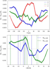 |
Fig. 2 Distribution of residuals between ten synthetic fields and SNYMG samples across the position space (top panel) and the LSR tangential velocity space (bottom panel). Dashed lines indicate the mean velocities of known open clusters according to the MOCA database. |
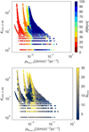 |
Fig. 3 Resulting Kmin,0.99 for all the hyper-parameter combinations as a function of the RPS density threshold |

3.4 Identifying NYMG candidates in real over-densities
We ran the detection algorithm on the ten Sc samples, considering over-densities with α ≥ 0.99 as significant detections, as explained in Sect. 3.3. The results consist of a list of statistically significant over-densities for each hyper-parameter combination. Some over-densities may be detected in several combinations of hyper-parameters, so we developed in this section a criterion to choose among the different detections.
We used the Bayesian Information Criterion (BIC; Schwarz 1978) to fit a set of multivariate Gaussians to each over-density in the RPS. This allows us to identify different substructures of a single NYMG in the RPS and reduce the level of field star contamination in the groups. Each star for the original overdensity is assigned to the Gaussian it most likely belongs to. Then, we compute for each member of the group the ratio rc = f (r, u)/f(rmean, υmean), where f (r, u) corresponds to the probability density function (PDF) of the fitted Gaussian evaluated on the RPS position of the member and f (rmean, υmean) to the PDF evaluated on the mean RPS position of the Gaussian. Although this ratio is not a probability, it tells us how likely it is that a star belongs to the distribution based on its RPS position relative to the mean position of the Gaussian, which has by definition the highest likelihood of belonging to the Gaussian. We can then compute for each group the score function as
 (2)
(2)
where N is the number of members in the group. The more tightly grouped the members of a group are and the more members a group has, the higher its score. We consider all the different groups detected in all the hyper-parameter combinations and identify the one with the highest C. Then, we discard all the other groups that contain at least one of the members of the group with maximum C. We iterate this process over the remaining groups until all the stars are either assigned to a group or discarded. Finally, we identify from our final list of groups the ones that contain at least ten members of one of the known NYMGs. We follow all the previous steps for each of the ten Sc samples and merge the results into one final list of detected NYMGs.
3.5 NYMG candidates from this work
Following the procedure presented in Sect. 3.4, we detected a total of 1705 over-densities. As discussed in Sect. 3.3, overdensities that are statistically significant when compared to the Besançon field might still not be significant relative to the full field, a result of the real non-axisymmetric potential of the Milky Way; alternatively, it might simply be substructures of other stellar associations different from the NYMGs. As shown in Appendix F and following the approach from Ratzenböck et al. (2023), we fitted a double Gaussian to the univariate distribution of over-density sizes from which we estimated that only 473 (~28%) of the detected over-densities are more likely to be real.
We found that 35 of the 1705 detected over-densities include members of 47 of the 68 groups from SLit. Only 2 of these 35 over-densities do not belong to the likely real 473 overdensities. The first of those over-densities corresponds to the group ETAC, while the other corresponds to a fragment of RATZSCO12. We detected however another over-density with members from RATZSCO12 that does belong to the likely real 473 over-densities. By discarding the 2 known over-densities corresponding to ETAC and the fragment of RATZSCO12, we end up with 33 over-densities corresponding to 44 known NYMGs (~65% of the 68 known groups), whose general statistics are shown in Table 1. Although the list of the remaining 440 over-densities is interesting, it is very likely that many are associated with sub-structures of massive old moving groups or star-forming regions. A more detailed analysis of these overdensities will be presented in a separate publication. In this work, we focus on studying only the 33 detected over-densities corresponding to the 44 recovered group candidates. As pointed out in the MOCA database, in numerous cases, it is not clear whether NYMGs with similar photometric and kinematic distribution are indeed separate associations or just sub-structures of a common association. This could be the reason why in many cases our detection algorithm classified different NYMGs from MOCA as part of a single group, leading to this shorter list of 33 group candidates instead of a list of 44 groups.
Our detection algorithm classified the known groups TAUMGLIU9 and GRTAUS9B from Slit as one group which we call TAUMGLIU-GRTAUS. This means that the sources classified by our algorithm as candidate members share a common region of the RPS. Similarly, our detection algorithm detected the following group candidates that merge different sets of known NYMGs from MOCA: RATZSCO23 and GRSCOS27C as GRSCOS-RATZSCO-A; ETAU and MUTAU as EMUTAU; TAUMGLIU7 and TAUMGLIU8 as TAUMGLIU-A; THOR and 118TAU as THOR-118TAU; GRTAUS9B and TAUMGLIU9 as TAUMGLIU-GRTAUS; RATZSCO-28 and GRSCOS10 as GRSCOS-RATZSCO-B; TAUMGLIU18, TAUMGLIU19 and HSC1368 as TAUMGLIU-HSC; GRTAUS3A and GRTAUS3B as GRTAUS3; and TAUMGLIU15, TAUMGLIU20 and TAUMGLIU21 as TAUMGLIU-B. In all of these cases, we find that the Slit members of the MOCA groups of each detected group share a common sequence in the CMD, likely corresponding to young isochrones.
In the specific case of EMUTAU, we notice that the Slit members of the MOCA group MUTAU are more scattered in the CMD than the members of EMUTAU. We observe a similar behaviour for TAUMGLIU9 within TAUMGLIU-GRTAUS, HSC1368 within TAUMGLIU-HSC, and GRTAUS3A within GRTAUS3. In each one of these cases, our detection algorithm alone does not provide the necessary tools to conclude if the different MOCA groups within each detected group are indeed separate physical associations or just sub-structures of the same association. In the case of RATZSCO23 and GRSCOS27C, for example, it has been shown that these are likely to be separate groups (Kerr et al. 2021; Ratzenböck et al. 2023); however, their similar ages and proximity in phase-space make it difficult for our algorithm to differentiate between them. Additionally, as a consequence of our algorithm prioritising purity over recovery by design, the spread of these two groups in the CMD along their respective potential isochrones may have been diminished, leading to an even more important degeneracy for our method.
We detected a total of 7530 candidate members across the identified groups. To lower the level of contamination from field stars, we discarded the source candidates with rc < 0.1, leaving only 4166 (55% of all detected candidates) source candidates in the final set of recovered NYMG candidates. The value of the threshold on rc was chosen by testing which value would maximise the amount of discarded MS stars that are photometrically older than 100 Myr and minimise the amount of discarded stars from the PMS. To identify stars older than a certain age A on the MS, we simply selected stars from the MS that are below the turn-on locus on the CMD where the isochrone of age, A, transitions from the PMS into the MS. Figure 1 shows the mass and MG of the turn-on of different isochrones as an example. The initial list of the 7530 candidate members including the final list of 4166 candidate members as well as the general statistics and information of the groups from Table 1 is available at the CDS.
Figure 4 shows a CMD distribution of all the 4166 detected candidate members from this work. We can see that the ages from MOCA correlate well with sequences that are very likely to be isochrones. This means that each of the detected NYMG candidates appears to follow an isochrone on the CMD, which strongly suggests that stars of a same NYMG were born together. We also notice that the group candidates are mostly distributed into three age categories: the youngest groups with ages around A ~ 10 Myr, the middle-aged groups with A ~ 40 Myr, and the old groups with A ~ 90 Myr.
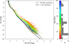 |
Fig. 4 CMD distribution of all the 4166 candidate members detected in this work. The colour map shows the age of the identified groups according to MOCA. The black solid and dashed curve show the 1 Gyr and 100 Myr isochrones, respectively. The rotated histogram shows the distribution of the detected NYMG ages according to MOCA. The ageaxis of the histogram is the same as the colour bar axis. |
3.6 Estimating the purity and recovery rates of the NYMGs
We estimated the recovery rate, fr, of each group candidate as the fraction, ndet,lit/nlit, where ndet,lit corresponds to the number of members of the group from Slit detected as members of the group with rc > 0.1 and nlit corresponds to the total number of members of the group from Slit. We found a total fr relative to the 44 recovered groups of 44% and an average fr per group of 59%. Figure 5 shows the fr of each group as a function of distance. If we ignore the groups that are part of the Sco-Cen complex, we see that on average, fr appears to increase with heliocentric distance. This can be explained partially by the fact that groups that are closer to the Sun appear more scattered in the sky, leading to a higher dispersion in sky tangential velocities, which makes the detection of their members more challenging. Although the values of fr may seem low for the closest recovered NYMGs, these values are based on the members from the literature, so the presence of any contamination in the literature members that would have survived the selection made in Sect. 2.3 will lower the real recovery rates. Regarding the groups from the Sco-Cen complex, we notice that they cover a large range of recovery rates (∆ fr ~ 0.6) for a short range of distances (∆d ~ 60 pc). However, we can notice that the mean fr of the groups from the Sco-Cen complex does follow the trend of the other groups.
Figure 6 shows the CMD of the candidates from Slit, the 7530 original source candidates from this work with rc > 0, and the recovered source candidates. We can see that many of the sources from Slit and the original 7530 candidates from our work are located in the MS locus, some of which are located below the turn-on of 100 Myr. Some of those stars might very likely correspond to field star contaminants. To test this possibility, we fitted a Gaussian to each NYMG from Slit in the RPS and selected the sources with rc > 0.1. In the case of the Slit members, we find that ~51% of the MS stars have rc < 0.1 while only ~38% of the PMS stars have rc < 0.1. Similarly, in the case of the original 7530 detected candidates from this work, we find that ~76% of the MS stars fulfil the condition rc < 0.1 and ~55% of the PMS stars have rc < 0.1. The latter statistic tells us that for both the Slit sample and the detections from this work, the rc parameter suggests that stars from the MS tend to be more scattered than the ones from the PMS. A first potential explanation could be that older groups tend to be more kinematically scattered than younger groups, but we do not notice from Table 1 any correlation between the age and the purity rate fp of the groups, which quantifies the fraction of candidate members that are true members. We present the method to estimate fp in Sect. 3.6. A second more likely explanation could be that these statistics are simply a consequence of the fact that the fraction of field contaminants in the MS is way higher than in the PMS. If this is the case, it means that the rc > 0.1 threshold is a good criterion to lower the level of contaminants within the detected groups.
Based on the previous analysis, we computed a likely less contaminated recovery rate  where the subindex 0.1 indicates the threshold rc > 0.1 on the Slit members. With this new recovery rate, we estimated a total fr,0.1 of 71% and an average fr,0.1 of 54% per cluster. Additionally, we can estimate the level of purity of each group according to the literature as fp,0.1 = ndet,lit,0.1/ndet,lit. This purity parameter measures the fraction of recovered sources with rc > 0.1 over the number of recovered sources. We obtained a total fp,0.1 of 76% and a mean fp,0.1 of 81% per group.
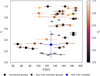 |
Fig. 5 Recovery rates, fr, as a function of the mean distance of each detected group. The colour indicates the purity rate, fp. The dots correspond to all the recovered groups that are not part of the Sco-Cen complex while the crosses correspond to the ones that do belong. The blue dot indicates the mean recovery of the Sco-Cen complex groups. |
4 IMF of selected NYMGs
In this section we infer the individual IMFs of the 33 detected NYMGs from the Sc samples as well as the individual IMFs of the 44 recovered groups based on their members from the Slit sample. This involves the estimation of masses for the member candidates and the stars added for completeness using the GSFs. We first show how to infer masses of the individual sources from their photometry and parallaxes. Then, we present the resulting IMFs of each group after correcting them for contamination due to field stars in each mass bin and compare them with the IMFs from the Slit members. Finally, we obtain the mean-normalised IMFs of the detected and recovered groups and compare them to each other and to results from the literature.
4.1 Inferring individual masses and ages
For a source with an apparent magnitude, G, colour BR = BP - RP, measured parallax ϖ, assumed extinction vector A = (ABR, AG), and assumed age A, we can infer its true parallax ϖ0, true extinction A0 and mass m by following Bayes’ rule:
 (3)
(3)
Assuming an agnostic prior on ϖ0 and A0 we have that P(m, ϖ0, A0) = P(m), which is by definition our a priori assumption of the IMF. We can then infer the mass alone by marginalising on ϖ0 and A0:
 (4)
(4)
Assuming that G, BP, RP, and ϖ have Gaussian errors, and that for a given NYMG the distribution of AG and ABR are Gaussian, we can then approximate the likelihood as a product of normal distributions:
 (5)
(5)
where oi ∈ {G, BR, ϖ, AG, ABR}. In this notation, oi corresponds to the measured or assumed parameter, while oi,0 corresponds to the value being inferred or integrated. In the particular cases of G0 and BR0, these are functions of m, ϖ0, A0, and the age A computed as

and

where MG,A(m), MBP,A(m), and MRP,A(m) are the mass-magnitude relations for Gaia passbands interpolated from the isochrone of age A resulting from the combination of the same models used for the isochrones presented in Sect. 2.1 (Baraffe et al. 2015; Marigo et al. 2017; Phillips et al. 2020).
To infer mass from observables {G, BR, ϖ, AG, ABR}, we used Eqs. (4) and (5) assuming for the prior the Chabrier (2005) system IMF, described by a log-normal distribution with a characteristic mass mc — 0.2 M⊙ and σ — 0.6 for masses lower than 1 M⊙, and a Salpeter (1955) power-law for higher masses. We consider this model because it is representative of disc stellar populations with unresolved stellar systems (Hennebelle & Grudić 2024). For the extinctions, we used the mean extinction AV and its standard deviation estimated for each NYMG from the 3D maps from Gontcharov (2017), and used it to estimate the corresponding values in Gaia bands following the same procedure presented in Sect. 2.1.
With this method, if we know the age, A, of a star, we can simply find the mass, m, that maximises the posterior. In this work, we used the ages from MOCA reported in Table 1 to infer the masses.
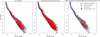 |
Fig. 6 MG vs BP-RP CMD of the candidate members of the NYMG candidates before applying the rc > 0.1 cut (grey dots), highlighting the sources that are discarded with this cut (red crosses). The dashed lines indicate the 100 Myr (blue line) and 1 Gyr (black line) isochrones. Top, middle, and bottom plots correspond, respectively, to the members according to the candidates of S lit, the candidates of the detected groups from this work, and the exact match between the two latter samples. |
4.2 Accounting for contamination
The Sc sample corresponds to SNYMG corrected for incompleteness due to most observational biases. Then, the resulting IMFs are already corrected for these incompletenesses. We present here the correction of the IMFs for contamination from the overlap of Besançon field stars and NYMGs in the RPS. To estimate the fraction of contaminants per mass bin for each group, we start by identifying the source candidate members of the group that were classified by the DBSCAN as core-points using the hyper-parameter combination used for the detection of the group. Then, we generate a synthetic field from the model built in Sect. 3.3 and select the synthetic sources that are classified by the DBSCAN as neighbours of the core points of the group. We infer the masses of these synthetic stars using the same isochrones used to infer the masses of the source candidates of the NYMG and measure in each bin of mass ∆m the purity fraction as  , where
  and nfield,∆m are the number of source candidates and synthetic sources, respectively. We interpolate the purity as a function of mass and repeat the whole process for 200 random synthetic fields. Finally, we compute the average purity function fp(m) of the 200 fields and smooth it using a Gaussian Kernel at 1-σ. As shown in Table 1, we estimated an average purity per NYMG of (fp) of 86% and a total purity of 84%, which are similar values to the values of fp,0.1 estimated from the Slit recovered members.
Figure 7 shows the purity curves fp(m) for each of the 33 detected NYMG candidates as well as the mean (fp)(m), which, in most cases, shows between one and three minima. More particularly, (fp) shows two local minima. For a given group, we expect to encounter higher contamination in mass ranges corresponding to the most populated loci of the CMD that survive the photometric isochrone selection of the detection algorithm. We observe in Fig. 1 that apart from the MS, there are two other loci with a high density of stars. The first is located in the locus between the 0.1 M⊙ and 0.3 M⊙ evolutionary tracks, which corresponds to the characteristic mass range of the typical IMF of field stars in the solar neighbourhood. This peak in density can be explained by the fact that since the magnitude M of a star is proportional to the logarithm of its luminosity, L, and if we assume that its luminosity is proportional to a power of the mass, then we have M ∝ log(m), which implies that if the typical IMF of the solar neighbourhood field stars shows a peak around the characteristic mass, we should also see a peak in the CMD around the locus associated with the evolutionary tracks of such mass. The second region of high density corresponds to the locus between the ~30 Myr turn-on and the 1 Gyr turn-off where many isochrones older than 1 Gyr intersect the isochrones younger than ~30 Myr. These two loci of high density in the CMD could explain why one of the minima of (fp)(m) is located around the peak of the field IMF and the other one right after the 30 Myr isochrone turn-on. Additionally, for a given isochrone, we should also expect contamination around its turn-on as it is the closest MS locus of that isochrone to the peak of the field IMF. Depending on the age of the isochrone and, thus, on how close its turn-on is to the peak of the IMF and the locus between the ~30 Myr turn-on and the 1 Gyr turn-off, the contamination caused by the turn-on may blend with the fp minimum associated with one of the other two highly dense loci or simply produce a new fp minimum.
We notice that some fp(m) curves predict very high rates of contamination with minima as low as ~0.2 in certain mass ranges. Although such contamination may be true, it could also be explained by the fact that the synthetic fields used to estimate fp(m) do not include the presence of RPS over-densities produced by massive moving groups and open clusters but have the same number of objects as in Sc, as discussed in Sect. 3.3. This means that in regions of the RPS where there are no massive stellar associations, our model of the field will over-estimate the density of stars. Similarly, fp(m) will tend to underestimate the contamination in regions of the RPS that are close to some massive stellar association. The impact of under-or overestimating fp(m) is hard to predict as it is case-dependent, but we discuss this in Sects. 4.3 and 4.4.
Finally, contamination can also be produced by extinction as some stars from the MS that share kinematics with a younger group could be reddened and dimmed in the CMD towards the isochrone of the group. However, since our model of the Besançon field of stars is based on GOG, whose distribution in the CMD and phase space is based on Gaia photometric errors, the effect of extinction is encoded in our model of the field. This means that our estimation of purity already considers the effect of extinction.
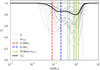 |
Fig. 7 Purity functions, fp(m), estimated from the simulated fields for all the detected NYMGs (grey curves) and the mean purity, (fp(m)) (black curve). The red, blue, and green vertical dashed lines indicate respectively the 0.08 M⊙, 0.2 M⊙, and the masses of the TO of the different ages used to photometrically select the NYMGs. |
4.3 Resulting IMFs
We estimated the IMF distribution by computing the KDE of the mass distribution of each group using a Gaussian kernel and a bandwidth of dlog10(m/M⊙) = 0.1. We consider this bandwidth because of a combination of factors: it corresponds to the typical mass bin size used in the literature to represent mass functions with histograms, and 95% of the errors on the inferred masses of all the source candidates are smaller than this value. We then estimated the IMF of each group as Φ(m) = Φ′(m)fp(m), where Φ′(m) corresponds to the KDE of the original mass distribution. The final reported IMF is the one corrected by the purity curves: Φ(m). Finally, we used the mean square error to fit a log-normal  to the KDE Φ(m) in the mass range mmin < m < 1 M⊙ and a power-law φ(m) ∝ mα in the mass range 1 M⊙ < m < mmax. Here, mmin and mmax are defined as the points where Φ(m) falls below ~0.54. This threshold is the result of the fact that, with a Gaussian KDE bandwidth of 0.1, a single object produces a normal distribution whose PDF at μ ± 2σ is ~0.54. Continuity was not imposed between the two parametrisations. Table 1 shows the fitted parameters mc, σc, and α of the inferred IMFs of the 33 detected groups.
Figure 8 shows the inferred IMFs for the particular cases of groups β-Pictoris (BPMG), EMUTAU, and TAUMGLIU-GRTAUS with their corresponding purity functions fp (m). As a comparison, we also show the IMFs we inferred considering only the members from Slit. We computed the KDEs of these mass distributions and parametrised them in the same way as we did for our detections. For each group, we show their respective purity function fp (m) as well as the recovery rates as a function of mass fr(m). These three individual cases illustrate some of the different cases found among the 33 groups. The same plots for the remaining 30 groups are shown in Appendix G.
For the specific case of BPMG, we detected only 56 candidate members, 36 of which are also reported in Slit as candidate members of BPMG. Meanwhile, this group according to Slit is made of 137 candidate members. Although we obtained similar parametrisations in the low-mass regime (m < 1 M⊙) using our detections and the members from Slit, we notice that in the high-mass range (m > 1 M⊙) the fitted power-law is steeper for the IMF inferred from the Slit members than for our detections. Moreover, the slope (α = −2.36 ± 0.13) obtained from our detections is much closer to the typical Salpeter (1955) slope of αSalpeter = −2.35 than the one estimated from the Slit candidates (α = −3.30 ± 0.13). The discrepancy in the high-mass regime between the parametrisations based on our detections and the candidate members from Slit could be explained by the fact that the IMF based on our detection was corrected using fp (m). Indeed, the latter function presents a minimum around 1 M⊙, preventing contaminants from the turn-ons of the isochrones with ages between 10 and 30 Myr mentioned in Sect. 4.2 from increasing the number of sources in that mass range, which would have led to a steepening of the slope. This means that the steepening of the slope in the case of using the candidates from Slit could be explained by the presence of contaminants forming a bump on the IMF around the solar mass. From now on, we refer to this bump as the 1 M⊙ bump.
In the case of EMUTAU, we found similar parametrisations between our detections and Slit in the whole mass range with similar number of candidate members. Moreover, we notice for the Slit members that the shape of the combined distribution of e-Tau and μ-Tau is representative of the distributions of the individual groups. Compared to the typical solar neighbourhood IMF (σc = 0.6), we found narrow characteristic widths (0.40 ± 0.17 and 0.35 ± 0.16 for our detections and the Slit members respectively) in the low mass regime. This is most likely due to a lack of brown dwarfs and other low mass objects. Such incompleteness is most likely due to the observational bias that we lack some of the faintest objects in SNYMG because of their low S/N, so that many of those sources did not make it through the selection process from Sect. 2.1. Indeed, if we directly interpolate the MG-mass relationship from the isochrone with the average age of e-Tau and μ-Tau (~55 Myr) and use it to estimate the mass of a star with the minimum G magnitude in SNYMG (~20 mag) and at the distance of EMUTAU’s closest member (~120 pc), we find that the minimum mass we could obtain this way for an EMUTAU member is ~0.05 M⊙. This explains why the IMF of this group based on both our detections and Slit drops very rapidly for masses m < 0.08 M⊙. In the high mass regime, we obtain shallow slopes (−1.76 ± 0.16 and −1.56 ± 0.15 for our detections and the Slit members respectively). This flattening can be explained by the presence of a higher amount of high mass stars than what is predicted by the typical αSalpeter. Although the fp(m) curve suggests that there is almost no contamination from the Besançon field, this does not necessarily imply that the potential excess of high mass stars we detected is real as it could simply be the product of contaminants from other more massive clusters.
Finally, the case of TAUMGLIU-GRTAUS is a typical case in which we may have over-estimated the contamination rate over the whole range of mass, as we can see from Fig. 8 where fp(m) gets as low as fp(m) ~ 0.4. This potential over-estimation of contamination could explain why we obtained for our detections a steeper slope (α = −2.55 ± 0.07) than αSalpeter. We also notice the presence of a bump on the IMF around m ~ 0.05 M⊙. This may be explained by the fact that the purity curve starts to drop at that mass to fp(m) ~ 0.5, which means that this bump is probably not real, but rather a consequence of an over-estimation of the contamination rate for masses higher than 0.05 M⊙ or an underestimation for lower masses. This potential over-estimation of contamination may be a consequence of the fact that this group covers a large region of the RPS, which makes it more likely to capture synthetic stars from our model of the Besançon field during our estimation of fp (m).
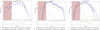 |
Fig. 8 Characteristic inferred IMFs which illustrate the different cases found among the 33 groups: β-Pictoris (left panel), EMUTAU (middle panel), and TAUMGLIU-GRTAUS (right panel). Solid and dashed lines in the bottom panels show respectively the purity and recovery functions. The dots with error bars correspond to the histogram of the distributions with Poisson error bars using log10(0.1 M⊙) bins. The smooth solid curves correspond to the KDEs of the masses using a Gaussian Kernel and bandwidth of log10(0.1 M⊙). The areas of both the histogram and the KDE are normalised to the total number of members of the group. The green solid line correspond to the IMF of the synthetic sources of Sc detected as members of the groups. The grey solid curves correspond to the IMFs of the individual MOCA groups for the cases of EMUTAU and TAUMGLIU-GRTAUS. The dashed lines in the top panels represent the log-normal and power-law parametrisation of the KDE. Black and blue colours correspond to the results based on the members from Slit and our detections respectively. The brown region represents the mass range of brown dwarfs (m ≲ 0.08 M⊙).The value of the fitted parameters are indicated in the legend. In the cases where more than one NYMG from MOCA was detected, we show their individual IMFs in grey, while the total IMF is in black. |
4.4 What the parametrised IMFs tell us
Although some maxima and minima in the inferred IMFs could be explained by potential contamination or incompleteness, others could simply be the result of Poisson noise since many groups present a low number of source candidates, which can highly affect the estimated parameters. Additionally, as shown with three different groups in Sect. 4.3, each group has its own specific reasons to show potential contamination or incompleteness in different mass ranges. To decrease the impact of Poisson noise and identify systematic behaviours in the IMFs of the NYMGs, we normalised the 33 inferred IMFs based on our detections to their respective areas and computed the mean-normalised IMF. The resulting IMF, together with its parametrisation and the individual normalised IMFs are shown in Fig. 9. We also show the mean-normalised IMF of the S lit members and as a visual guide the typical IMF of the solar neighbourhood as a Chabrier (2005) log-normal for m < 1 M⊙ and a Salpeter (1955) powerlaw for higher masses. The latter was built based on the 44 individual MOCA groups that we recovered rather than the 33 combined groups based on our detections. The mean-normalised IMF tells us on average what is the shape of the IMF of the NYMGs. We note that, given the ages and the typical number of members in the NYMGs, it is unlikely that they host massive stars which have already evolved off the main sequence. Therefore, the mean-normalised IMF provides a representative average shape without significant bias from evolutionary depletion at the high-mass end. Additionally, since the mean-normalised IMF of the NYMGs is well described by Salpeter (1955) slope in the high mass range, it is very likely that the number of high mass stars that are members of the NYMGs and that are not included in Gaia DR3 based on what was discussed in Sect. 2.1 is very low if not zero. Hence, our results suggest that these potentially missing O and B stars should not significantly affect our results.
As we can see in Fig. 9, the mean-normalised IMF of our detections is very smooth in the whole mass range. This is also the case of the mean-normalised IMF of the Slit members. However, we do notice in both cases a very slight bump between ~0.8 and ~1 M⊙. This bump may correspond to the 1 M⊙ bump that is the product of contamination from some of the turn-ons of the NYMGs as discussed in the specific case of β-Pictoris in Sect. 4.3. We notice that the bump for our detection is less significant than for the Slit members, which supports the idea that this bump is indeed the product of contamination since the IMFs based on our detections were corrected using the fp (m). This also suggests that our method to estimate contamination on average corrected well for the contamination from the turn-ons in our detections.
As in the cases of the individual IMFs, we fitted a log-normal and a power-law in the low (m < 1 M⊙) and high (m > 1 M⊙) mass ranges, respectively. We obtained parameter values mc = 0.25 ± 0.16 M⊙, σc = 0.45 ± 0.17, and α = −2.26 ± 0.09 for the mean-normalised IMF based on our detections and mc = 0.22 ± 0.14 M⊙, σc = 0.45 ± 0.17, and α = −2.45 ± 0.06 for the one based on the Slit members. We notice that the high mass range slope is slightly steeper for the Slit members than for our detections. This difference may be produced by the potential contamination of the 1 M⊙ bump, whose effect was lowered by the fp (m) curves in the case of our detections, as discussed previously. Additionally, the slope based on our detection may be shallower than αSalpeter because of cases similar to EMUTAU, as discussed in Sect. 4.3. However, the difference between the parametrisation of our detection and the one of the Slit members is still very small, and both cases are only one standard deviation away from αSalpeter. The combined IMF can also be decently described by a three-segment power-law function, analogous to Kroupa’s (Kroupa 2002) representation of the field IMF. For this parametrisation, we obtained slope values of 2.03 ± 0.02 in the low mass range m < 0.1 M⊙, −0.22 ± 0.05 in the intermediate mass range 0.1 < m/M⊙ < 1, and −2.26 ± 0.09 in the high mass range m > 1 M⊙. This parametrisation helps us uncover more accurately a potential incompleteness in the low mass range that is also visible from comparing the normalised typical solar neighbourhood IMF with the mean-normalised IMFs. Indeed, we notice that the estimated slope in the low mass range is much steeper than the one (−0.3) found by Kroupa (2002). The origin of this potential incompleteness may partially come from observational biases imposed by the selection process from Sect. 2.1. One example of this is shown for the case of EMUTAU in Sect. 4.3 where we show that the completeness in the lowest mass range is greatly affected by the distance of the group which leads to very low values of S/N for the apparent magnitude of the less massive objects of the group. Additionally, this potential incompleteness could also be partially explained by strong chromospheric activity from low mass objects. As summarised by Suárez et al. (2017) based on López-Morales (2007) and Stassun et al. (2014), intense chromospheric activity of low mass stars and brown dwarfs could either lead to underestimated masses due to lowered effective temperatures or to overestimated masses due to increased luminosities. However, the authors conclude that the mass differences should be of only ~5%, which is why we conclude that such phenomena should not have a significant impact on our estimation of the IMF.
Figure 10 shows Fig. 1 of the IMF review from Hennebelle & Grudić (2024) on top of which we have added the parametrisation of the mean-normalised IMF of both our detections and the Slit groups. In this figure, Γimf = α + 1. As discussed in Hennebelle & Grudić (2024), this plot shows that roughly seventy years of studying the IMF in the solar neighbourhood reveal a consistent trend. Although the inferred parametrisation of individual young stellar clusters and associations can vary significantly due to intrinsic differences or observational biases, the overall IMF exhibits a certain regularity. On average, it is well described by the parametrisation of the system IMF of field stars in the solar neighbourhood, as estimated by Chabrier (2005) in the low-mass range and by Salpeter (1955) in the high-mass range. Whether this behaviour is a consequence of a locally invariant IMF for populations in the solar neighbourhood or even the Milky-Way disc is not known. We do know, however, that it partially depends on whether the differences between individual IMFs are dominantly produced by intrinsic physical differences or by observational biases.
We notice in Fig. 10 that the mean-normalised IMF of both our detections and the S lit members are essentially identical to the average IMF of the solar neighbourhood, especially for the values of mc and α, while the parametrisation of the individual IMFs shown in Table 1 are consistent with the variety of estimations observed in Fig. 10 for young clusters. While the standard deviation for both mean-normalised IMFs (σc = 0.45 ± 0.17) is consistent with the typical value for the solar neighbourhood (σc ~ 0.6), we note that the slightly narrower absolute value could be due to incompleteness in the very low mass range 0.02 < m/M0 < 0.1 as it was previously discussed when comparing the fitted triple power-law with the parametrisation from Kroupa (2002). In the case of our detection, the potential overestimation of contaminants when using the purity rates fp (m) for some of the groups may have also contributed to narrowing the IMF. Apart from this small difference in σc and if we extrapolate the previously discussed statistical behaviour of the IMFs of young populations of the solar neighbourhood, we can conclude that the striking similarity between the parametrised mean-normalised IMF of our detections and the IMF of Chabrier (2005) and Salpeter (1955) is a strong argument in favour of the idea that, on average, there is no systematic bias in either our detections or the overall literature reflected by MOCA in the mass range 0.1 < m/M⊙ < 10 with the exception of the 1 M⊙ bump due to potential contamination discussed previously.
Figure 11 shows the distribution of the estimated parameters mc, σc, and α based on our detections, the Slit groups and their respective mean-normalised IMFs. As in the case of the mean-normalised IMFs, we observe that the distribution of parameters in the low-mass range from our detections (0.02 < m/M⊙ < 1) is similar to the one based on the Slit groups.
Regarding the high-mass range (m > 1 M⊙), we also notice similar distributions when using our detections and Slit. Additionally, we notice that in both cases the distribution is bimodal with a greater maximum around Salpeter (1955) slope and a lower maximum around α ~ −1. The maximum associated with shallower slopes is mainly the product of groups such as EMU-TAU that show an excess of massive stars, which could be the product of contamination from other stellar clusters. We also notice an extended tail with a third smaller local maximum around α 4.5. As discussed in the case of β-Pictoris, these steep slopes may be the product of contamination from the 1 M⊙ bump or from a lack of massive stars. However, we notice fewer cases with steep slopes for the IMFs based on our detections than for the ones based on Slit, which suggests that we have successfully reduced the contamination from the 1 M⊙ bump for the IMFs based on our detections.
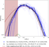 |
Fig. 9 Normalised individual IMF KDEs of the 33 groups (blue transparent curves), the mean-normalised IMF from our detections (blue solid curve), and from the Slit groups (black). The dots with Poisson error bars show the mean-normalised histogram of the masses of the groups and the dashed curves show the log-normal and power-law parametrisations of the mean-normalised IMFs. The green curve shows the mean-normalised IMF of the synthetic sources. The thick blue transparent lines show the triple power law fitted to the mean-normalised IMF of our detections. The brown dashed line shows the typical IMF of the solar neighbourhood: Chabrier (2005) log-normal for m < 1 M⊙ and Salpeter (1955) power-law for higher masses. |
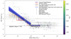 |
Fig. 10 Figure taken from Hennebelle & Grudić (2024) review on the IMF overlapped with the parametrisation of the mean-normalised IMF based on our detections (blue lines and shaded region) and the Slit members (black lines and shaded region). The plot shows the slope of different estimation of the IMFs of several populations in the Milky Way disc as a function of the stellar mass from the literature. The shadowed region corresponds to the propagated errors in the estimation of the parameters of the mean-normalised IMF of the NYMGs. |
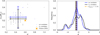 |
Fig. 11 Estimated parameters of the inferred IMFs from our detections (blue) and the groups from Slit (black). The thick, non-transparent blue and black dots on the left panel and the dashed lines on the right panel indicate the values of the mean-normalised IMFs. The left plot shows the estimated values (transparent dots with error bars) for the parameters of the log-normal with the values from the parametrisation made by Chabrier (2005). The right plot shows the distribution of the power-law slopes estimated through a KDE with the value found by Salpeter (1955). |
5 Summary, conclusions, and discussion
This work presents the first inference of the IMFs for a large set of NYMGs, a crucial step toward understanding the origin of these groups. In this section, we summarise and discuss our main conclusions, covering the tools and methods developed, the detected NYMG candidates, the inferred IMFs, and the implications for the origin of these groups.
5.1 Tools and methods
In this work, we developed the following methods and tools:
A general method to estimate the completeness of a sample within a given survey, based on the survey’s selection function and the criteria used to define the sample. We applied this method to enhance the completeness of our initial sample using the GaiaUnlimited selection functions.
A detection algorithm that combines the DBSCAN clustering method with GDR3 astrometric and photometric data to identify stellar co-moving groups and estimate the statistical significance of each detection through a comparison with the GOG synthetic catalogue.
A simple Bayesian method to infer the masses and ages of GDR3 sources classified as NYMG members, using their parallaxes, photometry, and extinction. Although the individual masses of the candidate members of the detected NYMGs were inferred assuming a mean extinction vector, we do not expect the inferred masses to differ significantly from those obtained using individual extinctions because the overall extinction is very small. Finally, we adopted stellar models that are typically employed in IMF studies. A systematic comparison with alternative models, while important, is beyond the scope of this work.
5.2 The detected NYMG candidates
Following our search for NYMGs using our detection algorithm, we report the following results:
We detected of a total of 473 over-densities in the RPS, 33 of which correspond to group candidates associated with at least one of the 44 of the 68 NYMGs listed in MOCA. Since this work focused only on the recovered known groups, the remaining over-densities will be studied in future works. The 33 NYMG candidates include a total of 4166 candidate members, of which 2545 are new members. In a few cases, different groups from the literature were detected as a single group candidate by our detection algorithm and our method cannot distinguish whether they are separate populations with similar properties or substructures of the same association. However, we do notice shared ages and CMD distribution for groups that were merged by our detection algorithm.
The 24 remaining NYMG candidates from the Slit sample that we did not recover present Slit members that are either too scattered in the RPS or have too few members, resulting in a low RPS density that our method could not detect.
We achieved a recovery rate relative to the literature between 44% and 54% with a mean recovery per group between 59% and 71%. We estimate that only 16% to 24% of our candidate members are contaminants. A conservative detection strategy was adopted by maximising the C score function and applying a threshold of rc > 0.1, due to the RPS scattering introduced by the use of tangential velocities. This likely reduced the recovery rates of the known groups but significantly minimised contamination. We prioritised purity over recovery with the aim of prioritising statistical representation over completeness in number, because the goal of this work is to infer the IMF shape of the NYMGs, rather than identify all members of these groups.
We found that the members of the detected NYMG candidates follow sequences likely associated with young isochrones in the CMD and that their ages are mostly distributed into three categories: young (~10 Myr), middleaged (~40 Myr), and old (~90 Myr).
We showed for all groups that for both our detections and the Slit members, MS candidate members tend to be more kinematically scattered than the PMS candidates. This is reflected in both cases by a higher percentage of stars with rc < 0.1 in the MS than in the PMS. This result could be a consequence of two non-excluding potential phenomena. The first is the possibility that older groups would tend to be more scattered than younger groups. The second is that older groups are more likely to have old star contaminants, as they are closer to the MS, and this contamination would increase the RPS dispersion of their host groups. Further information on radial velocities and chemistry is essential to confirm memberships of individual sources and, hence, to infer how the previously mentioned phenomena contribute to what we observe.
5.3 Inferred IMFs of NYMGs
For the 33 detected groups, we inferred the individual masses of their candidate members and their corresponding IMFs in the mass range 0.02 ≲ m/M⊙ ≲ 10. Our findings are as follows:
We present the IMFs of 33 NYMG candidates (Table 1). Previous studies have constructed IMFs for only three of the 68 known NYMGs listed in MOCA: TW-Hya (TWA), Volans-Carina (VCA), and Tucana-Horologium (THA). In addition to estimating the IMFs of these three groups, we provide the first IMF estimates for the remaining 30 detected NYMGs.
We parameterised the individual IMFs of the 33 detected groups, as well as the mean-normalised IMF, using a lognormal function for m < 1 M⊙ and a power-law for m > 1 M⊙. The parameters of the mean-normalised IMF from our detections (mc = 0.25 ± 0.17 M⊙, σc = 0.45 ± 0.17, and α = −2.26 ± 0.09) and the Slit candidate members (mc = 0.22 ± 0.14 M⊙, σc = 0.45 ± 0.17, and α = −2.45 ± 0.06) are both consistent with the typical system IMF of the solar neighbourhood estimated by Chabrier (2005) and Salpeter (1955). This result suggests that there is no significant systematic bias in our detections and the members from Slit based on our discussion of Fig. 10.
Our method to estimate and correct for contamination significantly reduced the 1 M⊙ bump around the turn-on of most of the NYMGs, which is likely associated with contamination as shown in Fig. 7. Importantly, while this method helps to identify contamination rates from the Besançon field within the inferred IMFs, it does not identify which specific candidate members are contaminants. This is why the presence of the bump is slightly more visible for the IMFs based on Slit, for which no contamination correction was applied. This translates into a slightly steeper slope for the IMF based on Slit than for the one based on our detections.
5.4 Hints on the origin of the NYMGs
Our results provide important insights into the origin of the NYMGs. The most significant conclusion is that the striking similarity between the mean-normalised IMF of the NYMGs and the typical system IMF of stellar clusters and field stars in the solar neighbourhood (e.g. Bastian et al. 2010), in the mass range 0.1 < m/M⊙ < 5, together with the fact that most NYMGs follow sequences in the CMD likely corresponding to young isochrones, supports the hypothesis that NYMGs are remnants of disrupted clusters or associations potentially in the process of dispersing.
The weak signatures of the NYMGs in the RPS and phasespace suggest that they could be unbound. To explore this possibility, we performed a simple estimation of the lower bounds, Qmin, for the virial ratio, Q = T/|U|, for each group, defined as Qmin = Tmin/|U|. Here, U denotes the total potential energy of the group, while Tmin is the total kinetic energy computed without the radial velocities of individual sources (using only vα,LSR and υδ,LSR). Since T > Tmin, it follows that Qmin < Q. For the detected groups we find 1.3 < Qmin < 1.4 × 10³, implying Q > 1 for all groups. This simple estimate of Qmin therefore suggests that the studied NYMGs are not gravitationally bound. A similar analysis was performed by Suárez et al. (2019) on the young (5 < age/Myr < 10) 25-Ori group, showing that it is gravitationally unbound. If the NYMGs are indeed unbound, this raises the intriguing possibility that younger groups such as 25-Ori could represent NYMG-like progenitors. Nevertheless, the present results are not sufficient to draw a firm conclusion on this matter, which will require a deeper analysis beyond the scope of this work.
Furthermore, the IMF similarities indicate that if dispersion is occurring in the NYMGs, it does not preferentially affect a specific stellar-mass range within 0.1 < m/M⊙ < 5. However, our results do not allow us to draw conclusions for m < 0.1 M⊙. If we assume that the IMF is invariant across the Galactic disc and resembles the system IMF of the solar neighbourhood, then, as discussed in Sect. 4.4, the estimated slope (2.03 ± 0.02) in the mass range, m < 0.1 M⊙, would imply a deficit of low-mass objects relative to the slope (0.3) from Kroupa & Bouvier (2003). Based on the discussion in Sect. 4.4, however, a substantial fraction of this apparent deficit is very likely due to observational biases. If, on the other hand, such an incompleteness proved to be real and independent of observational biases, it would imply that the scattering process of the NYMGs may have undergone a rapid mass-segregation phase. The present results are not sufficient to distinguish between these two scenarios.
Finally, it is important to note that the idea of the NYMGs being remnants of stellar clusters and associations does not rule out the possibility that they are also shaped by dynamical resonances with the Milky Way’s spiral arms or bar, such as other more massive and/or older groups (Antoja et al. 2010). An intriguing scenario to explore is that different stellar associations and clusters could be brought together in phase-space through such resonances in a short period of time. If this is the case for two populations of similar ages, distinguishing them from each other in the CMD should be difficult, if not impossible. If their ages differ significantly, this could result in double sequences in the CMD. In such cases, the second sequence produced by the MS stars that we observed in some cases might, in fact, correspond to genuine NYMG members rather than contaminants. Photometry alone would not suffice to determine whether this is the case or not. Even chemical abundances might fail to break this degeneracy if the two populations are chemically similar to begin with. These considerations will motivate future studies involving dynamical simulations of stellar clusters interacting with spiral arms and the bar to investigate whether resonant processes could indeed bring together remnants of different young stellar clusters or associations and produce NYMG-like associations.
Data availability
Table 1 and the catalogue of detected members are available at the CDS via https://cdsarc.cds.unistra.fr/viz-bin/cat/J/A+A/706/A370.
Acknowledgements
The author RB gratefully acknowledges the scholarship Becas de apoyo a docentes para estudios de posgrado en la Udelar, Maestría, 2022 from the Comisión Académica de Posgrado (CAP) as well as the McCarthy-Stoeger Fellowship from the Vatican Observatory Foundation for financially supporting and making possible this work. Likewise, RB and JJD thank the Programa de Desarrollo de Ciencias Básicas (PEDECIBA) and the Apoyo de Movilidad Individual Académica (MIA) of the Universidad de la República (UdelaR, Uruguay) for their financial support. RB and GS also thank the Heising-Simons Foundation for its support, particularly; RB acknowledges grant # 2022-3927 from the foundation. CRZ acknowledges support from programs UNAM-DGAPA-PAPIIT IN101723 and IN107226. This work made use of the high-performance computing facilities of ClusterUY (Nesmachnow & Iturriaga 2019), for which the authors are thankful. The authors extend their deep gratitude to Anthony Brown for the enriching comments and advice provided through their early review of this manuscript. The authors thank Ronan Kerr as well as the referee of this article for cautiously reviewing this work and providing very kind and helpful comments. Finally, they warmly thank Luis Aguilar, Mauro Cabrera, Bruno Domínguez, Pau Ramos, and Rodrigo Cabral for closely following this work from its early stages and for sharing their wisdom and insights, some of which were key to the development of this research.
References
- Antiche, E., Masana, E., Julbe, F., & Borrachero, R. 2014, in EAS Publications Series, 67-68, 355 [Google Scholar]
- Antoja, T., Figueras, F., Torra, J., Valenzuela, O., & Pichardo, B. 2010, in Lecture Notes and Essays in Astrophysics, 4 (ICE, Univ. Barcelona), 13 [Google Scholar]
- Astropy Collaboration (Price-Whelan, A. M., et al.) 2022, ApJ, 935, 167 [NASA ADS] [CrossRef] [Google Scholar]
- Bailer-Jones, C. A. L. 2015, PASP, 127, 994 [Google Scholar]
- Bailer-Jones, C. A. L., Rybizki, J., Fouesneau, M., Demleitner, M., & Andrae, R. 2021, AJ, 161, 147 [Google Scholar]
- Baraffe, I., Homeier, D., Allard, F., & Chabrier, G. 2015, A&A, 577, A42 [NASA ADS] [CrossRef] [EDP Sciences] [Google Scholar]
- Bastian, N., Covey, K. R., & Meyer, M. R. 2010, ARA&A, 48, 339 [Google Scholar]
- Campello, R. J. G. B., Moulavi, D., & Sander, J. 2013, in Advances in Knowledge Discovery and Data Mining, eds. J. Pei, V. S. Tseng, L. Cao, H. Motoda, & G. Xu (Berlin, Heidelberg: Springer Berlin Heidelberg), 160 [Google Scholar]
- Castro-Ginard, A., Brown, A. G. A., Kostrzewa-Rutkowska, Z., et al. 2023, A&A, 677, A37 [NASA ADS] [CrossRef] [EDP Sciences] [Google Scholar]
- Chabrier, G. 2005, in Astrophysics and Space Science Library, 327, The Initial Mass Function 50 Years Later, eds. E. Corbelli, F. Palla, & H. Zinnecker (Springer), 41 [Google Scholar]
- Danielski, C., Babusiaux, C., Ruiz-Dern, L., Sartoretti, P., & Arenou, F. 2018, A&A, 614, A19 [NASA ADS] [CrossRef] [EDP Sciences] [Google Scholar]
- Dib, S. 2023, ApJ, 959, 88 [NASA ADS] [CrossRef] [Google Scholar]
- Ester, M., Kriegel, H.-P., Sander, J., & Xu, X. 1996, in Proceedings of the Second International Conference on Knowledge Discovery and Data Mining, 226 [Google Scholar]
- Fabricius, C., Luri, X., Arenou, F., et al. 2021, A&A, 649, A5 [NASA ADS] [CrossRef] [EDP Sciences] [Google Scholar]
- Fernández, D., Figueras, F., & Torra, J. 2008, A&A, 480, 735 [NASA ADS] [CrossRef] [EDP Sciences] [Google Scholar]
- Gagné, J. 2024, PASP, 136, 063001 [Google Scholar]
- Gagné, J. 2024, PASP, accepted [arXiv:2405.12860] [Google Scholar]
- Gagné, J., & Faherty, J. K. 2018, ApJ, 862, 138 [Google Scholar]
- Gagné, J., Faherty, J. K., Mamajek, E. E., et al. 2017, ApJS, 228, 18 [CrossRef] [Google Scholar]
- Gagné, J., Faherty, J. K., & Mamajek, E. E. 2018, ApJ, 865, 136 [Google Scholar]
- Gagné, J., Faherty, J. K., Moranta, L., & Popinchalk, M. 2021, ApJ, 915, L29 [CrossRef] [Google Scholar]
- Gaia Collaboration (Antoja, T., et al.) 2021a, A&A, 649, A8 [EDP Sciences] [Google Scholar]
- Gaia Collaboration (Smart, R. L., et al.) 2021b, A&A, 649, A6 [EDP Sciences] [Google Scholar]
- Gaia Collaboration (Vallenari, A., et al.) 2023, A&A, 674, A1 [NASA ADS] [CrossRef] [EDP Sciences] [Google Scholar]
- Gontcharov, G. A. 2017, Astron. Lett., 43, 472 [NASA ADS] [CrossRef] [Google Scholar]
- Hennebelle, P., & Grudić, M. Y. 2024, ARA&A, 62, 63 [Google Scholar]
- Hopkins, A. M. 2018, PASA, 35, e039 [NASA ADS] [CrossRef] [Google Scholar]
- Hunt, E. L., & Reffert, S. 2021, A&A, 646, A104 [NASA ADS] [CrossRef] [EDP Sciences] [Google Scholar]
- Kerr, R. M. P., Rizzuto, A. C., Kraus, A. L., & Offner, S. S. R. 2021, ApJ, 917, 23 [NASA ADS] [CrossRef] [Google Scholar]
- Kraus, A. L., Shkolnik, E. L., Allers, K. N., & Liu, M. C. 2014, AJ, 147, 146 [Google Scholar]
- Kroupa, P. 2002, Science, 295, 82 [Google Scholar]
- Kroupa, P., & Bouvier, J. 2003, MNRAS, 346, 369 [NASA ADS] [CrossRef] [Google Scholar]
- Lada, C. J., & Lada, E. A. 2003, ARA&A, 41, 57 [Google Scholar]
- Lindegren, L. 2018, Re-normalising the astrometric chi-square in Gaia DR2, gAIA-C3-TN-LU-LL-124, http://www.rssd.esa.int/doc_fetch.php?id=3757412 [Google Scholar]
- Lindegren, L., Klioner, S. A., Hernández, J., et al. 2021, A&A, 649, A2 [EDP Sciences] [Google Scholar]
- López-Morales, M. 2007, ApJ, 660, 732 [Google Scholar]
- Luhman, K. L. 2021, AJ, 163, 24 [Google Scholar]
- Malzer, C. & Baum, M. 2020, in 2020 IEEE International Conference on Multisensor Fusion and Integration for Intelligent Systems (MFI) [Google Scholar]
- Marigo, P., Girardi, L., Bressan, A., et al. 2017, ApJ, 835, 77 [Google Scholar]
- Nesmachnow, S., & Iturriaga, S. 2019, in Supercomputing, eds. M. Torres, & J. Klapp (Cham: Springer International Publishing), 188 [Google Scholar]
- Offner, S. S. R., Clark, P. C., Hennebelle, P., et al. 2014, in Protostars and Planets VI, eds. H. Beuther, R. S. Klessen, C. P. Dullemond, & T. Henning, 53 [Google Scholar]
- Phillips, M. W., Tremblin, P., Baraffe, I., et al. 2020, A&A, 637, A38 [NASA ADS] [CrossRef] [EDP Sciences] [Google Scholar]
- Quillen, A. C., Pettitt, A. R., Chakrabarti, S., et al. 2020, MNRAS, 499, 5623 [CrossRef] [Google Scholar]
- Ramos, P., Mateu, C., Antoja, T., et al. 2020, A&A, 638, A104 [EDP Sciences] [Google Scholar]
- Ratzenböck, S., Großschedl, J. E., Möller, T., & et al. 2023, A&A, 677, A59 [NASA ADS] [CrossRef] [EDP Sciences] [Google Scholar]
- Rieke, G. H., & Lebofsky, M. J. 1985, ApJ, 288, 618 [Google Scholar]
- Rix, H.-W., Hogg, D. W., Boubert, D., et al. 2021, AJ, 162, 142 [NASA ADS] [CrossRef] [Google Scholar]
- Robin, A. C., Luri, X., Reylé, C., et al. 2012, A&A, 543, A100 [NASA ADS] [CrossRef] [EDP Sciences] [Google Scholar]
- Salpeter, E. E. 1955, ApJ, 121, 161 [Google Scholar]
- Schönrich, R., Binney, J., & Dehnen, W. 2010, MNRAS, 403, 1829 [NASA ADS] [CrossRef] [Google Scholar]
- Schwarz, G. 1978, Ann. Statist., 6, 461 [Google Scholar]
- Slesnick, C. L., Hillenbrand, L. A., & Carpenter, J. M. 2008, ApJ, 688, 377 [NASA ADS] [CrossRef] [Google Scholar]
- Stassun, K. G., Scholz, A., Dupuy, T. J., & Kratter, K. M. 2014, ApJ, 796, 119 [Google Scholar]
- Suárez, G., Downes, J. J., Román-Zúñiga, C., et al. 2017, AJ, 154, 14 [Google Scholar]
- Suárez, G., Downes, J. J., Román-Zúñiga, C., et al. 2019, MNRAS, 486, 1718 [CrossRef] [Google Scholar]
- Swiggum, C., Alves, J., Benjamin, R., et al. 2024, Nature, 631, 49 [NASA ADS] [CrossRef] [Google Scholar]
See also Danielski et al. (2018).
Appendix A Distance from the inverse of parallax
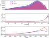 |
Fig. A.1 Top panel: Distribution of G magnitudes for the sample of stars with distances d = 1 /ϖ < 200 pc (solid line histograms) and distances dpg < 200 pc from Bailer-Jones et al. (2021) (shaded histograms). The blue histograms represent the S and Spg samples. The red histograms represent the SNYMG and SNYMGpg samples, as explained in Sect. 2.1. Middle panel: Residuals of the number of sources between SNYMG and S NYMGpg (red) and between S and Spg (blue) as a function of G. Bottom panel: Same residuals as the middle panel, shown as a function of the photometric S/N of G. All error bars correspond to the propagated Poisson error. |
Estimating distances using the inverse of parallax (dϖ = 1/ϖ) is the simplest but least precise method (Bailer-Jones 2015). On the other hand, the photo-geometric distances dpg estimated by Bailer-Jones et al. (2021) provide a more robust determination for the complete GDR3 catalog. We demonstrate in this section that these estimates show good agreement with dϖ = 1/ϖ when σϖ/ϖ < 0.1, where σϖ is the uncertainty in ϖ. Although smaller mean values of σϖ are expected for the solar neighbourhood compared to more distant regions due to the intrinsically larger ϖ and higher mean signal-to-noise ratio observations for nearby objects, the effect of the sample selection according to dϖ, particularly for the fainter sources, needs to be addressed.
We compare two samples: the one we call starting sample, which includes all stars having dϖ = 1/ϖ< 200 pc, and a sample we call GDR3dpg, which includes all stars having dpg < 200 pc. We applied the same procedures used to select the samples S and SNYMG from the starting sample (Sect. 2.1) to the GDR3dpg sample, producing the samples Spg and SNYMGpg, respectively. The number of sources for each sample is shown in Table A.1. The difference in number between the samples considering different distance estimations is smaller than 5% and occurs for stars with G > 17 mag, as shown in Fig. A.1. This difference increases with G as the S/N decreases. We conclude that, in our case, it is equivalent to estimate distances with either method.
Finally, we can estimate how many stars that truly belong to the solar neighbourhood MS and PMS with kinematics consistent with NYMGs are being discarded by the log10(S/NG) > 2.2 and σϖ/ϖ < 0.1 conditions mentioned in Sect. 2.1. To do so, we consider a new sample obtained by applying all the conditions used to build S with the exception of the σϖ/ϖ ≤ 0.1 and log10(FG/σFG) = 2.2 conditions to the match between the starting sample using dϖ and the GDR3dpg sample. Let  be the number of sources in that sample and Naux,match the number of sources in that sample after applying the S/N and σϖ/ϖ conditions. Then, we can roughly estimate the fraction of completeness after applying the S/N and σϖ/ϖ conditions as Naux,match/N*aux,match. We found that this ratio is equal to 0.987, which means that we are discarding only 1.3% of the sources of interest.
Number of solar neighbourhood sources from different samples selected from GDR3 following the prescription in Sect. 2.1 and using dϖ and dpg as estimates of distances as explained in Appendix A.
Appendix B Estimation of completeness
We present a general method to estimate the real completeness of a sample of stars based on the knowledge of the selection function of that sample. We consider a real and arbitrary set of stars called the real sample of interest, which in our particular case corresponds to the real solar neighbourhood MS and PMS stars with kinematics similar to that of the known NYMGs. Although the real sample of interest corresponds to the sample that we wish to study, it does not necessarily correspond to the one we end up studying in practice. The procedure for selecting candidate members of the real sample of interest from a given survey catalogue is generally made through the application of conditions that can be classified into two categories: selection conditions, which define the real sample of interest within the catalogue, and quality conditions, which do not define the sample of interest in itself but ensure some degree of quality in the data. In our specific case, one selection condition is ϖ ≥ 5 mas and one quality condition is ruwe ≤ 1.4.
If we assume that the number of contaminants in the sample resulting from applying all conditions is negligible, we can estimate the real completeness as  with ns∩q the number of sources selected using all the conditions and nreal the number of sources in the real sample of interest. An example of a contaminant source in our case could be a source with true parallax, ϖtrue < 5 mas, but with (poorly) measured parallax ϖobs > 5 mas, since it would not be excluded by the condition ϖ ≥ 5.
Although we do not know nreal and hence f, we can use the GSFs (Sect. 2.2) to estimate the real completeness in a given bin of observables ∆q, i.e. the fraction  . The real completeness fΔq can be estimated from the probability that a source within ∆q belongs to the studied sample resulting from applying selection and quality conditions, knowing that it belongs to the real sample of interest, by using Bayesian reasoning,
 (B.1)
(B.1)
Here, Sreal and Ss∩q represent the real sample of interest and the sample resulting from applying all conditions, respectively. In our case, Ss∩q corresponds to SNYMG.
Since we assumed the amount of contaminants in the studied sample Ss∩q is negligible, then almost all sources in Ss∩q ∩ Sreal should belong to the real sample, and hence the likelihood Pq(Sreal|Ss∩q) ~ 1. Regarding the prior Pq(Ss∩q), all sources from the studied sample belong to GDR3, hence Pq(Ss∩q) = Pq(Ss∩q ∩ GDR3) = Pq(Ss∩q|GDR3)Pq(GDR3). Finally, we can estimate the normalisation probability Pq(Sreal) as  , where
  is the real number of sources in the Universe (not only in the sample of interest) within Δq. We then notice that
  , where
  and
and  are the number of sources in Δq that belong to GDR3 and to the sample resulting from only applying the selection conditions, respectively. The latter ratio can be estimated as the probability Pq(Ssel|GDR3) with Ssel being the sample resulting from only applying selection conditions. In our case, Ssel corresponds to the ancillary sample S defined in Sect. 2.1. We can then rewrite Eq. (B.1) as
 (B.2)
(B.2)
All of the terms on the right side of Eq. (B.2) can be computed using the GSFs. Although this reasoning was made with the GSFs, we notice that the method can be generalised to any survey with a known selection function.
In practice, most quality conditions also act as selection conditions because they might discard sources that would have been wrongly included in the studied sample if they were not applied. In our case, for example, a source with true parallax ϖtrue < 5 mas but with (poorly) measured parallax ϖobs > 5 mas would not be excluded by the condition ϖ ≥ 5 mas but would be excluded after applying the condition σϖ/ϖ < 0.1. This means that the previously intended quality condition acted as a selection condition on this source in particular. We call conditions like this one mixed conditions. In the case of having mixed conditions, we cannot repeat the exact same reasoning because it would no longer be true that  . This is because we cannot know the number of contaminants that would have been included in the studied sample if we had only applied the selection conditions but that would have been discarded by a mixed condition. If we somehow know that this number is negligible, we can treat the mixed condition as a quality condition. If we cannot neglect such contaminants, we must treat the mixed condition as a selection condition and then use Eq. (B.2). In the latter case, this means we would not be accounting for the incompleteness produced by such mixed conditions.
Appendix C Selecting NYMGs from the MOCA database
We used the MOCA database to easily and efficiently identify known NYMGs from the literature. We started by querying all the associations in MOCA classified as moving groups with the query:
SELECT * FROM moca_associations WHERE physical_nature =’moving group’
The table moca_associations contains general information and comments on all the associations from MOCA. We then discarded groups when: their best estimated ages from the literature were above 100 Myr (age_myr > 100), their average distances to the Sun were greater than 200 pc (avg_dist > 200), or there existed another better definition of the group (subopti-mal_grouping ≠ 0), or the group could have been rejected for some reason (comments contains the strings Rejected, Not in BANYAN or Not included in BANYAN).
We then selected the individual sources of the identified NYMGs from the moca_associations table by querying calc_banyan_sigma using:
SELECT * FROM calc_banyan_sigma WHERE moca_bsmdid =23 AND max_observables = 1 AND moca_aid IN ({groupToSearch})
The calc_banyan_sigma table contains, for each source from MOCA, the results from running BANYAN, including membership probabilities. The condition moca_bsmdid =23 ensures selection of the latest results from BANYAN (ran in April 2025), and groupToSearch refers to the list of association names selected from moca_associations.
We discarded sources with membership probabilities lower than 0.95 (ya_prob < 95) and with distances to the Sun greater than 200 pc (d_opt > 200). We used unique source identifiers from different external surveys provided by MOCA to match the resulting sample to the following catalogues: Gaia DR1, DR2, and DR3, WISE, and 2MASS, prioritising in the case of multiple matches Gaia DR3 and DR2. Then, using Gaia proper motions, we propagated the sky positions of the Gaia sources from SNYMG back in time to the epochs of the other external surveys and sky-matched the catalogues. This allowed us to find sources from our query that had no GDR3 identifier but did have an identifier from another important survey. Only ~4% of the sources initially queried were not found in S NYMG.
Appendix D Kinematic biases and relevance of the LSR
Because the typical size of many NYMGs is similar to or even larger than their distance from the Sun, their proper motion distributions are expected to be affected by three phenomena: (i) NYMGs may cover very large regions of the sky, which means that even if all members of a NYMG share the exact same velocity vector, their proper motions may be different due to projection effects, (ii) two members of the same NYMG may be at different distances from the Sun, which means that even if they have the same sky position and Cartesian velocity vector, their proper motion vectors may differ, and (iii) the proper motions are also affected by the Sun’s motion in both the proper motion space and the tangential velocity space. Although it is not possible to correct the first bias without RV, the second bias can be addressed by computing the tangential velocity of each star using the parallax. To correct the third bias, it is necessary to work within the LSR.
Figure D.1 shows the distribution of proper motions and tangential velocities of known NYMGs from Slit in both the heliocentric frame and the LSR, obtained using the Astropy library (Astropy Collaboration 2022), which uses  km s−1 for the Sun’s motion from Schönrich et al. (2010). The kinematics in the heliocentric frame are more scattered than in the LSR, and the distribution of the NYMGs changes radically when going from proper motions to tangential velocities. Finally, we notice that the NYMGs tangential velocities in the LSR do not go beyond ~20 km s−1, which is consistent with the fact that these groups are made of very young stars deep within the disc kinematics. It is based on this plot that we decided in Sect. 2.1 to impose the condition
 ![Mathematical equation: $[v_{\alpha_{LSR}}^2+v_{\delta_{LSR}}^2]^{1/2} < 20$](/articles/aa/full_html/2026/02/aa57920-25/aa57920-25-eq35.png) km s−1.
km s−1.
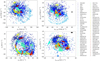 |
Fig. D.1 Distributions of proper motions (top panel) and tangential velocities (bottom panel) of known NYMGs in the heliocentric equatorial coordinate system (left panel) and the LSR equatorial coordinate (right panel). The black and grey filled ellipses on the right panels show how much the whole sample can be shifted due to respectively 1-σ and 2-σ uncertainties on the measurement of the LSR motion relative to the Sun, i.e. errors from Schönrich et al. (2010). |
Appendix E Setting the ε hyper-parameter in DBSCAN
Given that we are searching for NYMGs in both the position and the LSR tangential velocity space, we considered two different ε parameters: εr for the position space, and εv for the velocity space. Then, a possible approach, that we shall call approach A, is to apply the DBSCAN separately in the velocity space and then in the position space. In this approach, the two conditions that two stars with positions r0 and r1 and LSR tangential velocities υ0 and υ1 should meet to be considered neighbours are  and
and  . This approach is useful because it helps to reduce the field density by exploiting the fact that stellar groups in general are better defined in the velocity space than in the position space. Additionally, it allows us to estimate the minimum density of the detected group in both position (
 ) and velocity (
 ) spaces separately.
However, applying the DBSCAN separately is computationally more expensive than applying it only once to a fivedimensional space that combines positions and LSR tangential velocities. Fortunately, the conditions given by approach A can be approximated to a single condition by observing that both equations imply
 (E.1)
(E.1)
From here on, we call the approach that uses the DBSCAN in the SRPS through Eq. E.1 approach B.
We now introduce the similarity factor α that we use to define new scaling parameters  based on (εr,εv) through the equation
  . With these new parameters, we can now find the value of α that best approximates approach B using
  to the approach A with (εr, εv). We do so by finding the value of α that maximises the Jaccard similarity index defined as J = Vi/ Vu. Here, Vi and Vu correspond to the volumes of the intersection and the union, respectively, between the SRPS region defined by the equations of approach A using (εr, εv) and the SRPS region defined by Eq. E.1 through approach B using
  .
.
Using a Monte Carlo method to estimate the volumes Vi and Vu, we find that the value of α that maximises J is α = 0.847 with J = 0.654. With this change, we can re-write Eq. E.1 for approach B as
 (E.2)
(E.2)
Appendix F Over-density candidate rejection
To estimate which of the over-densities detected by our algorithm are more likely to be contaminants, we follow the approach described in Sect. 3.5.1 (see their figure 5) of Ratzenböck et al. (2023) and fitted a double-Gaussian to the uni-variate distribution of the over-density sizes. The Gaussian of lower mean value is likely to be dominated by contaminant detections while the second Gaussian is more likely to be dominated by real detections.
Figure F.1 shows the uni-variate distribution and the fitted normal distributions. As we can see, 1232 over-densities are rejected when using the intersection of the two normal distributions as criterion while 473 are not rejected. We also notice that only 5 of the over-densities associated with known NYMGs are rejected.
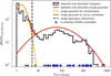 |
Fig. F.1 Uni-variate distribution of the over-density sizes (black histogram) with the double Gaussian fit (brown curve). The normal distributions of contaminants candidates and real over-density candidates are shown in orange and red respectively. The blue crosses indicate the number of members of the 33 detected group candidates associated with known NYMGs. The black dashed line shows where the two normal distributions intersect (Nover-densityy ~ 23). |
Appendix G IMFs of the detected NYMGs
All Tables
Number of solar neighbourhood sources from different samples selected from GDR3 following the prescription in Sect. 2.1 and using dϖ and dpg as estimates of distances as explained in Appendix A.
All Figures
|
Fig. 1 CMD of the starting sample (grey points) and the SNYMG sample (coloured scale indicating the density of points). The solid lines indicate the limits of the MS and PMS locus, the black dashed curves show the isochrones from Phillips et al. (2020), Baraffe et al. (2015), and Marigo et al. (2017) stellar evolutionary models for 10 Myr, 30 Myr, 100 Myr, and 1 Gyr. The horizontal black dash-dotted lines indicate the MG values corresponding to the turn-on (see Sect. 3.5) for the labelled masses. The red, orange, and blue dashed lines indicate the 0.1, 0.2, and 0.3 Μ⊙ evolutionary tracks, respectively. The red arrow indicates twice the extinction vector for an M4 dwarf star with AV = 0.22 mag. |
| In the text | |
|
Fig. 2 Distribution of residuals between ten synthetic fields and SNYMG samples across the position space (top panel) and the LSR tangential velocity space (bottom panel). Dashed lines indicate the mean velocities of known open clusters according to the MOCA database. |
| In the text | |
|
Fig. 3 Resulting Kmin,0.99 for all the hyper-parameter combinations as a function of the RPS density threshold |
| In the text | |
|
Fig. 4 CMD distribution of all the 4166 candidate members detected in this work. The colour map shows the age of the identified groups according to MOCA. The black solid and dashed curve show the 1 Gyr and 100 Myr isochrones, respectively. The rotated histogram shows the distribution of the detected NYMG ages according to MOCA. The ageaxis of the histogram is the same as the colour bar axis. |
| In the text | |
|
Fig. 5 Recovery rates, fr, as a function of the mean distance of each detected group. The colour indicates the purity rate, fp. The dots correspond to all the recovered groups that are not part of the Sco-Cen complex while the crosses correspond to the ones that do belong. The blue dot indicates the mean recovery of the Sco-Cen complex groups. |
| In the text | |
|
Fig. 6 MG vs BP-RP CMD of the candidate members of the NYMG candidates before applying the rc > 0.1 cut (grey dots), highlighting the sources that are discarded with this cut (red crosses). The dashed lines indicate the 100 Myr (blue line) and 1 Gyr (black line) isochrones. Top, middle, and bottom plots correspond, respectively, to the members according to the candidates of S lit, the candidates of the detected groups from this work, and the exact match between the two latter samples. |
| In the text | |
|
Fig. 7 Purity functions, fp(m), estimated from the simulated fields for all the detected NYMGs (grey curves) and the mean purity, (fp(m)) (black curve). The red, blue, and green vertical dashed lines indicate respectively the 0.08 M⊙, 0.2 M⊙, and the masses of the TO of the different ages used to photometrically select the NYMGs. |
| In the text | |
|
Fig. 8 Characteristic inferred IMFs which illustrate the different cases found among the 33 groups: β-Pictoris (left panel), EMUTAU (middle panel), and TAUMGLIU-GRTAUS (right panel). Solid and dashed lines in the bottom panels show respectively the purity and recovery functions. The dots with error bars correspond to the histogram of the distributions with Poisson error bars using log10(0.1 M⊙) bins. The smooth solid curves correspond to the KDEs of the masses using a Gaussian Kernel and bandwidth of log10(0.1 M⊙). The areas of both the histogram and the KDE are normalised to the total number of members of the group. The green solid line correspond to the IMF of the synthetic sources of Sc detected as members of the groups. The grey solid curves correspond to the IMFs of the individual MOCA groups for the cases of EMUTAU and TAUMGLIU-GRTAUS. The dashed lines in the top panels represent the log-normal and power-law parametrisation of the KDE. Black and blue colours correspond to the results based on the members from Slit and our detections respectively. The brown region represents the mass range of brown dwarfs (m ≲ 0.08 M⊙).The value of the fitted parameters are indicated in the legend. In the cases where more than one NYMG from MOCA was detected, we show their individual IMFs in grey, while the total IMF is in black. |
| In the text | |
|
Fig. 9 Normalised individual IMF KDEs of the 33 groups (blue transparent curves), the mean-normalised IMF from our detections (blue solid curve), and from the Slit groups (black). The dots with Poisson error bars show the mean-normalised histogram of the masses of the groups and the dashed curves show the log-normal and power-law parametrisations of the mean-normalised IMFs. The green curve shows the mean-normalised IMF of the synthetic sources. The thick blue transparent lines show the triple power law fitted to the mean-normalised IMF of our detections. The brown dashed line shows the typical IMF of the solar neighbourhood: Chabrier (2005) log-normal for m < 1 M⊙ and Salpeter (1955) power-law for higher masses. |
| In the text | |
|
Fig. 10 Figure taken from Hennebelle & Grudić (2024) review on the IMF overlapped with the parametrisation of the mean-normalised IMF based on our detections (blue lines and shaded region) and the Slit members (black lines and shaded region). The plot shows the slope of different estimation of the IMFs of several populations in the Milky Way disc as a function of the stellar mass from the literature. The shadowed region corresponds to the propagated errors in the estimation of the parameters of the mean-normalised IMF of the NYMGs. |
| In the text | |
|
Fig. 11 Estimated parameters of the inferred IMFs from our detections (blue) and the groups from Slit (black). The thick, non-transparent blue and black dots on the left panel and the dashed lines on the right panel indicate the values of the mean-normalised IMFs. The left plot shows the estimated values (transparent dots with error bars) for the parameters of the log-normal with the values from the parametrisation made by Chabrier (2005). The right plot shows the distribution of the power-law slopes estimated through a KDE with the value found by Salpeter (1955). |
| In the text | |
|
Fig. A.1 Top panel: Distribution of G magnitudes for the sample of stars with distances d = 1 /ϖ < 200 pc (solid line histograms) and distances dpg < 200 pc from Bailer-Jones et al. (2021) (shaded histograms). The blue histograms represent the S and Spg samples. The red histograms represent the SNYMG and SNYMGpg samples, as explained in Sect. 2.1. Middle panel: Residuals of the number of sources between SNYMG and S NYMGpg (red) and between S and Spg (blue) as a function of G. Bottom panel: Same residuals as the middle panel, shown as a function of the photometric S/N of G. All error bars correspond to the propagated Poisson error. |
| In the text | |
|
Fig. D.1 Distributions of proper motions (top panel) and tangential velocities (bottom panel) of known NYMGs in the heliocentric equatorial coordinate system (left panel) and the LSR equatorial coordinate (right panel). The black and grey filled ellipses on the right panels show how much the whole sample can be shifted due to respectively 1-σ and 2-σ uncertainties on the measurement of the LSR motion relative to the Sun, i.e. errors from Schönrich et al. (2010). |
| In the text | |
|
Fig. F.1 Uni-variate distribution of the over-density sizes (black histogram) with the double Gaussian fit (brown curve). The normal distributions of contaminants candidates and real over-density candidates are shown in orange and red respectively. The blue crosses indicate the number of members of the 33 detected group candidates associated with known NYMGs. The black dashed line shows where the two normal distributions intersect (Nover-densityy ~ 23). |
| In the text | |
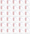 |
Fig. G.1 Same plots as Figure 8 for the remaining 30 detected groups. |
| In the text | |
Current usage metrics show cumulative count of Article Views (full-text article views including HTML views, PDF and ePub downloads, according to the available data) and Abstracts Views on Vision4Press platform.
Data correspond to usage on the plateform after 2015. The current usage metrics is available 48-96 hours after online publication and is updated daily on week days.
Initial download of the metrics may take a while.