| Issue |
A&A
Volume 707, March 2026
|
|
|---|---|---|
| Article Number | A252 | |
| Number of page(s) | 25 | |
| Section | Extragalactic astronomy | |
| DOI | https://doi.org/10.1051/0004-6361/202451460 | |
| Published online | 09 March 2026 | |
Detailed lens modeling and kinematics of the submillimeter galaxy G09v1.97
An analysis of CO, H2O, H2O+, and dust continuum emission
1
Department of Space, Earth & Environment, Chalmers University of Technology SE-412 96 Gothenburg, Sweden
2
Department of Physics, Institute for Computational Cosmology, Durham University South Road Durham DH 13LE, UK
3
School of Physics & Astronomy, University of Nottingham, University Park Nottingham NG7 2RD, UK
4
School of Mathematics, Statistics and Physics, Newcastle University Newcastle upon Tyne NE1 7RU, UK
5
School of Astronomy and Space Science, Nanjing University Nanjing 210093, China
6
Department of Physics & Astronomy, University of California Irvine Irvine CA 92697, USA
7
Sorbonne Université, UPMC Université Paris 6 and CNRS, UMR 7095, Institut d’Astrophysique de Paris 98bis Boulevard Arago 75014 Paris, France
8
Laboratoire d’Astrophysique de Marseille, Aix-Marseille Univ., CNRS, CNES Marseille, France
9
Instituto de Física y Astronomía, Universidad de Valparaíso Avda. Gran Bretaña 1111 Valparaíso, Chile
10
Astronomical Observatory Institute, Faculty of Physics, Adam Mickiewicz University ul. Słoneczna 36 60-286 Poznań, Poland
11
Leiden Observatory, Leiden University PO Box 9513 2300 RA Leiden, The Netherlands
12
National Radio Astronomy Observatory Charlottesville VA, USA
13
Millennium Nucleus for Galaxies (MINGAL) Santiago, Chile
★ Corresponding author: This email address is being protected from spambots. You need JavaScript enabled to view it.
Received:
11
July
2024
Accepted:
15
January
2026
Abstract
Context. While the formation mechanisms of intensely starbursting galaxies at high redshift remain unknown, one possible mechanism for producing these intense rates of star formation is via mergers and interactions. However, detecting these at high redshift remains a challenge. Observations of high-redshift gravitationally lensed galaxies provide a way to study the interstellar medium and environment of these extreme starbursts in detail.
Aims. We aim to use high angular resolution observations of dust continuum, CO(6−5), H2O(211 − 202), and H2O+(202 − 111) emission to constrain the ongoing processes in the z = 3.63 gravitationally lensed submillimeter galaxy H-ATLAS J083051.0+013224 (G09v1.97).
Methods. We used the sophisticated lens modeling software PYAUTOLENS to perform both parametric and nonparametric source modeling. We created a demagnified source plane CO(6−5) emission line cube and performed the kinematic modeling using 3DBAROLO. Additionally, we investigated the properties of the continuum and molecular line emission in the source plane.
Results. We find that the regions of CO(6−5) and H2O(211 − 202) emission are closely matched in the source plane, but that the dust continuum emission is more compact. We find that our lens modeling results do not require more than one source, contrary to what has been found in previous studies. Instead, we find that G09v1.97 resembles a rotating disk with Vmax/σ¯ = 2.8 ± 0.4, along with evidence of residual emission indicative of noncircular motions such as outflows, tidal tails, or an additional background galaxy.
Conclusions. We suggest that the origin of the noncircular motions might be associated with a biconical outflow or a tidal tail from an interaction; alternatively, this might indicate the possible presence of an additional galaxy. We calculated the dynamical mass, gas mass, star formation rate, and depletion time for G09v1.97, along with a high star formation rate and low gas depletion time. In combination, this suggests that G09v1.97 has recently undergone an interaction, triggering intense star formation, while also being in the process of settling into a disk.
Key words: galaxies: evolution / galaxies: high-redshift / galaxies: ISM / galaxies: kinematics and dynamics / galaxies: starburst
© The Authors 2026
 Open Access article, published by EDP Sciences, under the terms of the Creative Commons Attribution License (https://creativecommons.org/licenses/by/4.0), which permits unrestricted use, distribution, and reproduction in any medium, provided the original work is properly cited.
This article is published in open access under the Subscribe to Open model. This email address is being protected from spambots. You need JavaScript enabled to view it. to support open access publication.
1. Introduction
Some of the brightest and most strongly star-forming galaxies at high redshift are heavily dust-obscured galaxies (submillimeter galaxies, SMGs; Smail et al. 1997; Barger et al. 1998; Hughes et al. 1998; Dudzevičiūtė et al. 2020) and dusty star-forming galaxies (DSFGs; see reviews from Blain et al. 2002; Casey et al. 2014, and references therein). These galaxies have prodigious star formation rates (SFRs), prompting questions about the underlying formation mechanisms and the drivers behind such intense star formation. Overall, SMGs can reach total infrared (IR) luminosities of ∼1013 L⊙ and, in certain cases, they can maintain “maximum starbursts” of > 1000 M⊙ yr−1 (e.g., Barger et al. 2014; Simpson et al. 2015; Riechers et al. 2013). Consequently, these galaxies represent a crucial stage in the growth of massive galaxies, making them key to understanding the evolution of massive, high-redshift galaxies.
One process that is thought to lead to such intense SFRs and IR luminosities is mergers and/or interactions between high-redshift galaxies, where the molecular gas fuels the nuclear regions, triggering intense star formation (e.g., Mihos & Hernquist 1994; Hopkins et al. 2006; Engel et al. 2010). This is consistent with both simulations and observations of the high-redshift universe, which have shown the importance and high prevalence of mergers and interactions (e.g., Kereš et al. 2005; Hopkins et al. 2008; Genzel et al. 2010). However, some simulations suggest that these dusty starburst galaxies may form through more secular processes (e.g., Dekel et al. 2009; Davé et al. 2010). This is supported by observations of massive high-redshift galaxies that show no signs of merger or interaction activity, and only well-ordered rotation instead (e.g., Tacconi et al. 2013; Hodge et al. 2016; Jiménez-Andrade et al. 2018; Smit et al. 2018; Lelli et al. 2021; Roman-Oliveira et al. 2023). Although this phase represents a critical stage in galaxy growth, the formation mechanisms of these galaxies still remain uncertain.
One of the primary reasons for this lack of understanding is the difficulty inherent in observing high-redshift galaxies. Resolving the environment of high-redshift galaxies remains challenging, even for telescopes like the Atacama Large Millimeter Array (ALMA). SMGs have been shown to have an average redshift of ≈2.5 for those discovered at 870 μm (e.g., Chapman et al. 2005; Danielson et al. 2017), where an angular resolution of 1″ corresponds to ≈8.2 kpc. Even at an angular resolution of 0.1″, the physical scales probed within the galaxy would be at ≈800 pc scales. At this resolution, it is possible to begin to resolve the regions of denser and warmer gas (e.g., Tacconi et al. 2008; Riechers 2013; Spilker et al. 2015; Swinbank et al. 2015; Dye et al. 2015; Rybak et al. 2020, 2023), but surpassing this limit is challenging. Gravitational lensing circumvents the need for extremely high angular resolution observations. This phenomenon can, in effect, improve the angular resolution of observations by  , where μ is the lensing magnification factor (under the assumption that the magnification is static across the image), meaning that details within the interstellar medium (ISM) and environment can, in some cases, be resolved in the source plane.
To gain a better understanding of the processes governing SMGs, DSFGs, and other high-redshift galaxies with intense star formation rates, it is paramount to understand the internal ongoing processes in the ISM in detail, as well as the influence of the surrounding environment (i.e., mergers and interactions). In recent years, studies of the ISM of gravitationally lensed galaxies have shed considerable light on these processes (e.g., Amvrosiadis et al. 2025; Cañameras et al. 2018, 2021; Dye et al. 2022; Kade et al. 2023, 2024; Rybak et al. 2015, 2020, 2023; Spilker et al. 2022; Yang et al. 2019, 2023).
The strongly lensed SMG H-ATLAS J083051.0+013224 (hereafter, G09v1.97) at z = 3.63 is an ideal laboratory for studying the properties of high-redshift sub-millimeter galaxies. First reported in Bussmann et al. (2013), G09v1.97 is exceptionally bright in the IR with a lensing magnification factor of μ ∼ 6 − 10 and it has been studied in detail in a number of previous works (e.g., Bussmann et al. 2013; Yang et al. 2019; Maresca et al. 2022). G09v1.97 has an intrinsic IR luminosity of ∼1013 L⊙, and an SFR of > 1000 M⊙ yr−1, placing it among the most intense starbursts known to date. Yang et al. (2019) performed an in-depth study of G09v1.97 using ALMA data at an angular resolution of  and based on a parametric lensing model, they concluded that the source was composed of two merging and/or interacting galaxies.
The current paper utilizes very high angular-resolution ALMA observations ( ) of G09v1.97, achieving scales of a few hundred parsecs in the source plane, to study the ISM using the emission from the dust, CO(6−5), H2O(211 − 202), hereafter H2O and H2O+(202 − 111), hereafter H2O+. We present a nonparametric source plane reconstruction of the dust continuum emission and detected molecular line emission. Additionally, we discuss the implications of our findings as a result of the kinematic modeling we carried out. In Sect. 2, we describe the observations and data reduction steps. The results of the continuum and line analysis, lens modeling, and kinematic modeling are reported in Sect. 3. Section 4 provides a discussion of these results. Finally, our conclusions are presented in Sect. 5. Throughout this paper, we adopt a flat ΛCDM cosmology with H0 = 70 km s−1 Mpc−1, ΩΛ = 0.7, and Ωm = 0.3. At z = 3.63,
  corresponds to ≈740 pc in the image plane.
2. Observations and data reduction
G09v1.97 was observed in band 4 with ALMA as part of project ID 2018.1.01710.S (P.I. Yang). All calibrations and image processing were performed in the Common Astronomy Software Application package (CASA; McMullin et al. 2007). The band 4 observations were taken on 14-July-2019 using 41 antennas. The observations were performed using baselines between 138.5 m, and 8547.6 m, resulting in an angular resolution of  (using natural weighting). The on-source integration time was 47.2 minutes, with a total overhead time of 62.19 minutes. The overhead time includes the pointing, focusing, phase, flux density, and bandpass calibrations. J0825+0309 was used as the phase calibrator, J0725−0054 was used as the bandpass calibrator, and J0725−0054 was used as the flux calibrator. We report a conservative estimate of 10% to represent the uncertainty in the absolute flux calibration (noting that the fiducial value for band 4 is ∼5%)1. The weather conditions during the observations were good, with a mean precipitable water vapor of 0.8 mm and a phase root mean square (RMS) of 0.239°.
The data were calibrated using the ALMA interferometric pipeline (Hunter et al. 2023), including a calibration of the phase, bandpass, flux, and gain. The pipeline-reduced data were checked to ensure quality. The images produced by the pipeline data reduction of the calibrated data were inspected visually to ensure data quality and identify line-free channels to be used in continuum subtraction. Continuum subtraction was performed using the CASA task UVCONTSUB using a polynomial fit of order 1. Imaging of the calibrated data was performed in CASA using the TCLEAN task, cleaning in the region of expected emission using the mask encompassing the region of emission for the deep continuum and CO(6−5) emission images reported in Yang et al. (2019). Continuum images were created using the line-free channels and natural weighting. They were cleaned down to a 1σ level, where σ = 0.02 mJy/beam, at vsky = 154.5 GHz, corresponding to continuum emission at 1.94 mm. Similarly, spectral cubes were created from the continuum subtracted measurement set using natural weighting and were cleaned down to a 1σ level. The native spectral resolution of the observations was ≈7.8 MHz. To ensure a sufficient per-channel signal-to-noise ratio (S/N), we used a channel width of 20 km/s when cleaning the spectral cubes. We provide the details of the beam size, channel width, and image RMS in Table 1.
Details of the observations.
To be able to study the fainter H2O+ emission line, we combined the data presented above with lower-spatial-resolution observations (C36-5 configuration with baseline range 0.02−1.5 km) used in Yang et al. (2019, project ID: 2015.1.01320.S, P.I.: Omont). As the frequency setups for the two observational data sets differed, we searched for a common range of frequencies and then re-gridded the individual data sets to the common frequency range and a common spectral resolution of 15.625 MHz. Afterward, the individual data sets were combined to produce combined clean images. As a last step, and to correct for the intrinsic beam size differences in the combined data sets, we used the TP2VISTWEAK step from the Total Power to Visibilities tool (TP2VIS, Koda et al. 2011, 2019). Images from the combined data were cleaned and imaged using the CASA task TCLEAN using Briggs weighting with a robust factor of 0.5 to keep a reasonable balance between the S/N and angular resolution, while also maintaining an angular resolution as close to the higher resolution data as possible. We note that due to the significantly lower angular resolution of the combined dataset, it is only used to study the fainter H2O+ emission.
3. Results
3.1. Continuum emission
We detected strong continuum emission towards G09v1.97 at a ≈22σ level. We extracted the continuum from the region of expected emission from Yang et al. (2019), shown in Fig. 1. We find a 1.940 mm continuum flux of 7.00 ± 0.32 mJy. This value is lower than that found by Yang et al. (2019) of 8.8 ± 0.5 mJy, suggesting the possibility that some continuum emission has been resolved out in the high-resolution observations utilized in this paper. However, the extent of this discrepancy (20 ± 6%) is not large and, therefore, we did not consider it to have a significant impact on later results.
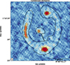 |
Fig. 1. Continuum image of G09v1.97, imaged using a natural weighting scheme. The contours are shown at −3, −2, 3, 4, 5, 6, 7, 8, 9, 10σ levels (σ = 0.02 mJy/beam). The black region shows the region from which the continuum emission was extracted. The synthesized beam is shown in the bottom- left of the image and corresponds to 0.11″ × 0.084″. |
3.2. Line emission
We detected CO(6−5), with a rest frequency of 691.4731 GHz, and H2O(211 − 202), with a rest frequency of 752.0331 GHz, in the high-resolution data. We did not detect H2O+(202 − 111)5/2 − 3/2 (rest frequency of 742.1531 GHz) in the high-resolution data and, thus, we used the combined dataset (as described in Sect. 2) for the analysis of the H2O+ line.
We performed a regional spectral extraction within the expected region of emission described in Yang et al. (2019). We used the same region of extraction for all species to enable consistent comparisons between them (region shown in black in Fig. 1). We did not detect any significant emission outside the region. We calculated the RMS for each species using a simple sampling method in which the RMS is sampled from distinct, emission-free regions of the cubes. We created moment-0 and moment-1 maps from the same region used to extract the spectra. For clarity, we removed flux at lower than 3σ levels in the moment-1 maps. The spectra for the H2O and CO(6−5), as well as the moment-0 and moment-1 maps, were created from the naturally weighted data to match images produced during the lens modeling, as described in Sect. 3.3. The H2O+ emission spectrum, moment-0, and moment-1 maps were created from Briggs-weighted images using a robust factor of 0.5 (see Sect. 2).
The integrated flux densities and line luminosities were calculated following Solomon et al. (1997) and expressed as
![Mathematical equation: $$ \begin{aligned} L_{\rm line} = (1.04 \times 10^{-3})\, I_{\rm obs}\, \nu _{\rm rest}\, D^{2}_{L}\, (1+z)^{-1} [L_{\odot }], \end{aligned} $$](/articles/aa/full_html/2026/03/aa51460-24/aa51460-24-eq7.gif) (1)
(1)
where Lline [L⊙] gives the luminosity of the emission line and Iobs is the velocity integrated flux density defined as Iobs = SlineΔV [Jy km/s], where Sline [mJy] is the observed flux density and ΔV [km/s] is the full width at half maximum (FWHM) of the emission line, νrest [GHz] is the rest-frame frequency of the line, DL is the luminosity distance [Mpc], and z is the redshift. Line properties for the emission lines detected towards G09v1.97 are provided in Table 2.
Line properties from our observations.
3.2.1. CO(6–5) emission
The spectrum of the CO(6−5) emission exhibits the same characteristic profiles as reported in Yang et al. (2019), with peaks in both the red (> 0 km/s) and blue (< 0 km/s) regions of the spectrum. The spectrum was fit with a double Gaussian profile to account for the asymmetric line shape. The ratio of the fitted peaks of the two emission lines from the Gaussian fitting is approximately peakred/peakblue ≈ 4.5 for CO(6−5). The flux of the CO(6−5) emission line was compared between the high-resolution ALMA dataset and the combined dataset, with no obvious difference observed (see Fig. A.1). This suggests that despite the very high resolution of the new CO(6−5) observations, no significant emission was resolved out.
A clear velocity gradient is seen in the moment-1 maps of the CO(6−5) data in the brightest regions of emission in the north and south of the image (see Fig. 3). This is further investigated later in the paper following lens modeling (see Sect. 3.4). We present the spectrum in Fig. 2 and the moment maps in Fig. 3.
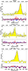 |
Fig. 2. Spectra of the detected molecular line species in G09v1.97. Top-left: CO(6−5) spectrum. Top-right: H2O spectrum. Bottom: H2O+ spectrum. Note: the H2O+ emission was not detected in the high-resolution data and, thus, the spectrum was taken from the combined data (as described in Sects. 2 and 3.2), resulting in a different spectral resolution than for the CO(6−5) and H2O emission. The spectrum for each molecule was extracted from a region corresponding to the region shown in Fig. 1. For each molecule, the spectrum is shown in the top panel, and the residuals from the Gaussian fits are shown in the lower panel. Single Gaussian profiles are shown in red, while double Gaussian profiles are shown in blue; similarly, in the lower panel, the residuals from fitting using a single Gaussian profile are shown in red and in blue for fits using two Gaussian profiles. It is clear that double Gaussian profiles offer a better fit of the spectra for all detected molecular line species. The dashed gray line in the top panel and the gray region in the lower panel represent the per-channel RMS. The top axis in the top panel for each spectrum shows the corresponding redshift. Note: the red residuals in the bottom panel are shown as slightly narrower (i.e., appearing to have a smaller channel width) than the blue, which is purely for clarity purposes. |
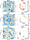 |
Fig. 3. Moment-0 and moment-1 maps of the molecular line emission detected towards G09v1.97. Top: CO(6−5). Middle: H2O. Bottom: H2O+. The contours are shown at −3, −2, 3, 4, 5, 6, 7, 8, 9, 10σ levels for the CO(6−5) and H2O emission and at −3, −2, 3, 4, 5σ levels for the H2O+ emission. The synthesized beam is shown in the bottom- left of every image, beam sizes can be found in Table 1 for each line. Note: the angular resolution is significantly lower for the H2O+ emission as it was imaged from the combined dataset as described in Sect. 2. A clear velocity gradient is visible in the moment-1 map of the CO(6−5) emission. |
3.2.2. H2O emission
The spectrum of the H2O emission also exhibits the same characteristic shape as previously reported (Yang et al. 2019) and closely matches the line profile of the CO(6−5) emission with the two peaks in the red and blue regions of the spectrum. We compare the normalized CO and H2O spectra in Fig. 4 to illustrate the similarity of the emission line profiles. Similarly to the approach taken for the CO(6−5) emission, we fit the spectrum with a double Gaussian profile to account for the asymmetric line shape. In comparison to the CO(6−5) spectrum, the peak in the blue part of the spectrum has significantly stronger flux. The ratio of the fitted peaks of the two emission lines from the Gaussian fitting is peakred/peakblue ≈ 2.3 for H2O. This is ∼1.5× smaller than the same ratio for the CO(6−5) emission, suggesting that the peak of the H2O emission in the red portion of the spectrum is lower, compared to its counterpart in the blue portion of the spectrum. This is further discussed in Sect. 4.1.
By contrast to the CO(6−5) emission, the velocity gradient in the image-plane moment-1 map of the H2O emission is much less prominent. This is likely due to the lower S/N of the H2O emission, in line with results reported in Yang et al. (2019), where similar velocity structures have been seen from a lower resolution data of CO(6−5) and the H2O data. Given the S/N of the CO data, we focus on the CO(6−5) emission when discussing the kinematics of G09v1.97. We present the spectrum in Fig. 2 and the moment maps in Fig. 3.
3.2.3. H2O+ emission
The spectrum of the H2O+ emission is at a sufficiently low S/N so as to be undetectable in the new, high-resolution observations. Instead, we used the combined data to improve on both the angular resolution and the S/N of the H2O+ emission. As in Yang et al. (2019), we found a similar line profile to that of the CO(6−5) and H2O emission with characteristic peaks in the red and blue regions of the spectrum, indicating that their spatial origins are comparable (Fig. 4). We show the normalized spectral comparison in Fig. 4. As with the CO(6−5) and H2O emission, we fit the spectrum using a double Gaussian profile to account for the asymmetric line shape. The ratio of the fitted peaks of the two emission lines from the Gaussian fitting is peakred/peakblue ≈ 7 for H2O+. This is about three times higher than the same ratio for the CO(6−5) emission and about five times than the same ratio for the H2O. However, it should be noted that the S/N of the blue component in the H2O+ spectrum is primarily below the noise level of the spectrum and, therefore, it is difficult to draw firm conclusions about the nature of this emission and the spectral shape.
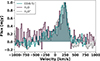 |
Fig. 4. Comparison of the normalized CO(6−5), H2O, and H2O+ emission. Note: the noise appears significantly higher in the H2O+ emission due to the line’s lower S/N value. The line profiles of all three emission lines are very similar. |
Similarly to the H2O emission, we do not detect a clear velocity gradient in the image-plane moment-1 map of the H2O+ emission. This is not surprising given the low S/N of the H2O+ emission and the low angular resolution of the images. Since the line profile of H2O+ is similar to that of the CO(6−5), we would expect to see an overall comparable kinematic structure. We present the spectrum in Fig. 2 and the moment maps in Fig. 3.
3.3. Lens modeling
Advanced lens modeling software, such as the publicly available Python-based code PYAUTOLENS (Nightingale 2016; Nightingale et al. 2018, 2021), allows for robust source-plane reconstructions of lensed galaxies. PYAUTOLENS has been used in a number of recent studies of high-redshift galaxies to determine the source-plane properties of the studied galaxies (Maresca et al. 2022; Zhang et al. 2023; Amvrosiadis et al. 2025). In this work, we utilized PYAUTOLENS to reconstruct the source plane emission of G09v1.97. PYAUTOLENS is capable of handling interferometric data and performing reconstructions directly on the visibilities, thereby minimizing the effect of correlated noise in interferometric images. Additionally, PYAUTOLENS can create source plane pixelizations from interferometric data, which eliminates the need to make assumptions on the background galaxy’s morphology. This approach is particularly advantageous for G09v1.97 as it does not require a priori assumptions to be made about whether the galaxy is a rotating disk or a merger. In its current form, intensity values from PYAUTOLENS fits performed on interferometric visibilities are in arbitrary units. While this does not impact our analysis, it is discussed in later sections when relevant. We also note that images produced by PYAUTOLENS are dirty images using approximately a natural weighting scheme.
3.3.1. Parametric source modeling
The SMG G09v1.97 is lensed by two galaxies with spectroscopic redshifts of z = 0.636 and z = 1.002, visible at optical wavelengths (Yang et al. 2019). We modeled these two galaxies as single isothermal ellipsoid (SIE) mass distributions. These mass profiles are characterized by their (x, y) offset from the phase center of the observations in arcseconds, Einstein radius, axis ratio (q), and position angle (PA). During the lens modeling, the redshifts of the lens galaxies were fixed, while we allowed all other parameters to vary, assuming uniform priors. The (x, y) offset and Einstein radius were allowed to vary around previously reported values from Yang et al. (2019) and Maresca et al. (2022). Although lens models have been successfully created for G09v1.97 using various lens modeling codes (e.g., Yang et al. 2019; Maresca et al. 2022), including PYAUTOLENS, discrepancies between different tools and observations necessitated allowing the parameters describing the lens mass models to vary rather than directly adopting values from previous works.
We modeled the source as a single Sérsic profile using a linear light profile, allowing the intensity parameters to be solved via linear algebra. This minimizes the degeneracy between parameters such as the intensity and the effective radius of the source. This model was parameterized by its (x, y) offset from the observation phase center, axis ratio (q), position angle (PA), effective radius, and Sérsic index. We note that the parametric modeling performed directly on the cleaned images reported in Yang et al. (2019) required multiple Sérsic source profiles to provide a good lens model. In this work, we do not find that we require more than a single source profile to obtain good lens models for each of the emission types, as described below.
We first modeled the dust continuum emission to obtain an optimized lens model and proceeded to use it to reconstruct the molecular line emission. We allowed all Sérsic parameters, including centroid coordinates, to vary in the fit to account for possible morphological differences between emission types. However, we note that the values found for different emission types are fairly consistent and are all within errors of each other. Further discussion regarding the extent of the different emission regions is reserved until Sect. 3.3.2 where the nonparametric source modeling is free from a priori assumptions.
We calculated the parametric modeling magnification errors through sampling the posterior distribution of the maximum likelihood solution for the lens mass model fit from the continuum data. We performed the sampling 1000 times for each emission type, obtained magnification factors for each of these samples, and calculated the standard deviation of the magnification factors from each sample, thus obtaining the magnification factor error. This approach is further utilized and described in Sect. 3.3.2.
3.3.1.1. Dust continuum emission.
We began by modeling the dust continuum emission using a parametric model for both lenses and the source to optimize the lens mass model. This optimized model is then extended to parametric models of the molecular line emission and nonparametric source modeling. The two lenses and the source profile were fitted as described above, with the best-fit lens mass model results provided in Table 3 and the best-fit source parameters in Table 4. The best-fit lens model yields a very good fit to the data, as shown in Fig. 5. Through this methodology, we obtain a lensing magnification factor of μcontinuum = 10.55 ± 0.26. This is in very good agreement with the magnification factor found by Yang et al. (2019) of μ = 10.2 − 10.5.
3.3.1.2. CO(6–5) emission.
To verify that our optimized lens mass model works well for the molecular line emission, we modeled the CO(6−5) emission using the continuum-optimized lens model (i.e., the lens model was fixed with parameters given in Table 3) and a single Sérsic profile for the source. The lens model derived from the dust continuum emission provided an excellent fit to the CO(6−5) emission, indicating that the lens model is optimal. We provide best-fit source parameters for the CO(6−5) emission in Table 4. We show the CO(6−5) image, model, and residual in Fig. 5. Through this methodology, we obtain a lensing magnification factor of μCO(6 − 5) = 9.72 ± 0.27.
Best-fit lens parameters, optimized from parametric models of the dust continuum emission.
Best-fit parametric source modeling results for continuum and detected molecular line species.
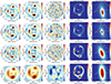 |
Fig. 5. Parametric lens and source modeling results for the detected emission towards G09v1.97. First row: Dust continuum. Second row: CO(6−5). Third row: H2O. Fourth row: H2O+ emission. The first column shows the dirty image as produced by PYAUTOLENS with contours shown at 3, 4, 5, 6, 7, 8, 9, 10σ levels, where 1σ is the rms of a blank region of the image. Note: this is not a cleaned image and structures may look slightly different than those shown in cleaned images. The second column shows the dirty model image as produced by PYAUTOLENS with contours shown at 3, 4, 5, 6, 7, 8, 9, 10σ levels. The third column shows the dirty residual image produced by PYAUTOLENS with contours shown at the −3, −2, 2, 3, 4, 5σ levels. The fourth column shows the image plane emission parametric model of the data produced by PYAUTOLENS. The white line represents the critical line. The fifth column shows the source plane emission parametric model of the data produced by PYAUTOLENS. The white line shows the caustic line. All images are centered around the ALMA phase center for each image. Note: the H2O+ emission is of significantly lower angular resolution as the lensing model was created using the combined data, as described in Sect. 2. |
We found a slight residual in both the northern and southern images of the source; see Fig. 5. These residuals are small, ≤3σ. We attempted to improve the model by including a second source, also described by a Sérsic profile and as motivated by Yang et al. (2019). However, the inclusion of this second source did not improve the residuals, and we discarded this model. We suggest that this residual is mainly due to the ‘clumpy’ nature of the CO(6−5) emission. Indeed, smoother image-plane emission in the dust continuum does not exhibit this residual emission. Therefore, we suggest that this residual is primarily due to limitations in the lens modeling itself, primarily the inability of a single, smooth (by definition) Sérsic profile to provide a fully realistic model of a galaxy. This is evident in the smoothness of the dirty model images from PYAUTOLENS; see Fig. 5. We suggest that nonparametric modeling would likely provide a better fit to the data and is explored in Sect. 3.3.2.
3.3.1.3. H2O emission.
Similarly to the CO(6−5) emission, we modeled the H2O emission using the continuum-optimized lens model and a single Sérsic profile for the source. We provide the best-fit source parameters in Table 4. We show the H2O image, model, and residual in Fig. 5. Through this methodology, we obtain a lensing magnification factor of μH2O = 11.60 ± 0.41.
Similarly to the CO(6−5) emission, we find a slight residual in the northern image of the source; see Fig. 5, at a ≈2σ level. We suggest the same explanation for this residual as for the CO(6−5) model and explore nonparametric models of the H2O emission in Sect. 3.3.2.
3.3.1.4. H2O+ emission.
Similarly to both the CO(6−5) and H2O emission, we modeled the H2O+ emission using the continuum-optimized lens model with a single Sérsic profile to describe the source. We show the H2O+ image, model, and residual in Fig. 5. Through this methodology, we obtained a lensing magnification factor of μH2O+ = 14.86 ± 0.48.
We note that the four different emission types have different magnification factors. The magnification factors reported here are the average across the source and are, therefore, dependent on the spatial extent of the source. Given that we did not impose constraints on the different emission types, the differential lensing between different emission types is to be expected2. A similar effect has been found in previous studies in which lens modeling was performed on both different line emission and dust continuum emission at different wavelengths (e.g., Giulietti et al. 2023; Perrotta et al. 2023).
3.3.2. Nonparametric source modeling
Previous studies of G09v1.97 have not included nonparametric source modeling results for molecular or atomic line emission. In this work, we use the optimized lens mass model derived from the dust continuum emission (described in Sect. 3.3.1) to create a pixelized reconstruction using a magnification weighted adaptive Voronoi pixel mesh. This approach has two main benefits: it imposes no constraints on the source morphology (apart from a regularization coefficient; see below) and maintains regions with higher magnification and, therefore, higher angular resolution. The reconstruction employs a regularization coefficient that corresponds to the smoothness of the image and attempts to balance between overfitting and oversmoothing (Nightingale et al. 2018). We used a constant regularization scheme parameterized by the regularization coefficient. This method has been employed in numerous recent studies to reconstruct high-redshift galaxies observed with ALMA and the James Webb Space Telescope (Maresca et al. 2022; Giulietti et al. 2023; Zhang et al. 2023; Perrotta et al. 2023; Amvrosiadis et al. 2025).
We used this methodology to create pixelized reconstructions of the dust continuum emission, CO(6−5), H2O, and H2O+ emission using a Voronoi mesh covering a circular region of radius 1.5 arcsec (11 kpc) in the image plane around G09v1.97. We show the images, models, and residuals for all modeled emission in Fig. 6. We find that the nonparametric source models provide a similarly good fit to the data as the parametric source models. We find small residuals at the same spatial regions as in the parametric models for the CO(6−5) and H2O emission. However, these residuals are found at lower significance (≈2σ levels) in the nonparametric models, suggesting that the nonparametric models provided an improved fit to the emission. Further, the discrepancies in the morphology between the parametric and nonparametric source plane models suggest that the parametric modeling should be viewed with caution as this is a likely indication that the emission contains structures not well represented by parametric models. We find that the nonparametric source plane morphology of the different emission types is very similar, with no indications of complex morphologies indicative of multiple sources. This provides further verification that there appears to be a single background source, not multiple sources, as found in Yang et al. (2019). We discuss the emission morphologies and extents further in Sect. 4.1.
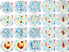 |
Fig. 6. Nonparametric source modeling results for the detected emission towards G09v1.97. First row: Dust continuum. Second row: CO(6−5). Third row: H2O. Fourth row: H2O+ emission. The first column shows the dirty image as produced by PYAUTOLENS with contours shown at 3, 4, 5, 6, 7, 8, 9, 10σ levels where 1σ is the rms of a blank region of the image. Note: this is not a cleaned image, and structures may look slightly different than those shown in cleaned images. The second column shows the dirty model image as produced by PYAUTOLENS with contours shown at 3, 4, 5, 6, 7, 8, 9, 10σ levels. The third column shows the dirty residual image produced by PYAUTOLENS with contours shown at −3, −2, 2, 3, 4, 5σ levels. The fourth column shows the image plane emission nonparametric model of the data produced by PYAUTOLENS. The black line shows the critical line. The fifth column shows the source plane emission nonparametric model of the data produced by PYAUTOLENS. The black lines show the caustic line. All images are centered around the ALMA phase center for each image. Note: the H2O+ emission is of significantly lower angular resolution as the lensing model was created using the combined data, as described in Sect. 2. |
Finally, we created source plane error maps for each of the emission sources. The source plane errors have two contributions: (i) the uncertainties on the lens mass model (σl) and (ii) the uncertainties on the source-plane pixelized reconstruction (σdata). The total source plane error map is then given by  . Here we describe how each contribution is determined.
We estimated the lens mass model errors (σl) by creating source plane pixelized emission maps for the CO(6−5) emission using lens mass models sampled from the posterior distribution of each of the lens parameters. We assume that the error on the lens mass model will not be significantly different for different emission types, and therefore only perform this sampling on the CO(6−5) emission3. Given that the formal statistical uncertainties in the lens mass model are small (see Table 3), we do not expect the contribution from (σl) to be significant. The reported errors on the parameters are comparable to those reported in Table 4 of Maresca et al. (2022), despite differences in the source modeling assumptions used in their analysis. Such small formal uncertainties are common in group-scale strong lenses like G09v1.97, particularly when adopting simple mass models, such as a singular isothermal ellipsoid (SIE), as they are prone to model misspecification. We sampled the posterior of the maximum-likelihood solution for the lens mass model (fit from the continuum data) 1000 times, thereby creating 1000 different samples of the CO(6−5) emission in the source plane. We then created the σl map by calculating the standard deviation of the brightness in each pixel across the 1000 samples. This approach is valid only if the lens model parameters form Gaussian distributions over the 1000 samples. We confirmed that this assumption holds.
We estimated the source-plane pixelized reconstruction error (σdata) by using PYAUTOLENS’s infrastructure. To estimate the uncertainty in our nonparametric source-plane reconstructions, we started by estimating the RMS noise for each pixel in the source plane. Assuming a fixed lens mass model, the RMS error in each pixel is derived from the diagonal elements of the covariance matrix, following Eq. (10) of Warren & Dye (2003). In our case, this matrix is computed directly from the interferometric visibilities in the uv-plane and corresponding visibility errors extracted using CASA’s STATWT task, as described in Eq. (8) of Enia et al. (2018). This approach gives us an RMS noise value for each Voronoi pixel in the source plane, which was then interpolated onto a regular square grid using the same method applied in the source reconstruction.
We show the total error map ( ) for each emission source in Fig. B.3. We have normalized the error maps by the maximum value in the intensity map, so the error maps can be effectively interpreted as a percentage error in each pixel. As expected, the contribution from the lens mass model errors (σl) are small and generally do not provide a meaningful contribution to the total error. The errors for both the continuum and H2O+ emission are, as expected due to the larger volume of data used for fitting, smaller than for the other emission types. Figure B.3 also provides signal-to-noise maps (i.e., intensity divided by intensity error) for clarity, in particular for later analyses performed in the paper. Generally, the emission in the source plane is at S/N ⪆ 3 meaning that the errors are generally modest. However, the outer regions of emission can be at significantly lower S/N. This is further discussed in Sect. 4.2.
Similarly to the parametric models, we calculated the magnification factor from the pixelized regime. The pixelization magnification factor error comes from sampling the maximum-likelihood lens model 100 times, and creating pixelized image and source plane emission maps for each sample where the magnification error is the standard deviation of the magnification factor across these 100 samples. We note that we only performed the posterior sampling 100 times due to time constraints when performing the reconstructions. Generally, the parametric vs. pixelized model magnification factors are similar, within ≈2σ, with the exception of the CO(6−5) emission where the magnification factor is stronger in the pixelized regime. We do not further investigate the magnification factor discrepancies from the two modeling regimes. For the purposes of this paper, we use the average of the magnification factors where relevant for magnification correction of physical properties.
3.3.3. Spectral cube reconstructions
We used the PYAUTOLENS’s nonparametric source modeling capabilities to create a source plane demagnified emission cube of the CO(6−5) emission. We limited this analysis to the CO(6−5) due to the very high per-channel S/N necessary to create robust demagnified cubes. Indeed, as the main goal of this analysis was to perform kinematic modeling on the demagnified cubes, the CO(6−5) emission was of primary interest.
To create demagnified source-plane emission cubes, we divided the emission line into bins of equivalent size and nonparametrically modeled the emission in each bin. We used a spectral resolution of ≈50 km/s, allowing for a reasonable balance between maintaining S/N in each bin while maintaining a high spectral resolution. The images for each bin were then interpolated onto a square pixel grid, a built-in capability of PYAUTOLENS, and combined to form a spectral cube. The interpolation to a square pixel grid resulted in the loss of nonstatic pixel size across the image, necessitating the adoption of a beam size for future kinematic modeling. We assumed a standard beam size of five pixels per source-plane beam, where the source-plane beam was defined as  , with μ given by the parametrically modeled CO(6−5) emission (see Table 4). Thus, the static angular resolution achieved in the source plane was approximately
  (≈260 × 200 pc) for the reconstructed CO(6−5) spectral cube.
The CO(6−5) reconstructed source plane cube was used to create moment-0 and moment-1 maps for the CO(6−5) emission, shown in Fig. B.2. These can be compared with moment-0 and moment-1 maps made on the nonstatic images, which utilize a Voronoi mesh. We computed moment-0 and moment-1 maps for the Voronoi pixels and visually verified that the interpolation to square pixels did not significantly affect the moment-0 or moment-1 maps. Therefore, for the remainder of the analysis, we use the reconstructed source plane cube with a static beam unless otherwise stated.
Similarly to the parametric modeling and the nonparametric models of the dust continuum and molecular line emission, we find no evidence of two sources in the moment-0 maps (Fig. B.2), contrary to the findings of Yang et al. (2019). Combined with the smooth velocity gradient seen in the moment-1 map (Fig. B.2), this indicates a single, rotating disk. This interpretation is further investigated in Sects. 3.4 and 4.2.
We show the error maps for the CO(6−5) emission line using the same method as described in Sect. 3.3.2. In this case, the σdata is a moment-0 map created from an error cube for the CO(6−5) using the visibility errors in each channel. We show the CO(6−5) source plane moment-0, total error moment-0, and S/N maps in Fig. B.3. We find that inner regions of the image are at ≥5 whereas the outer regions of the emission are at ≈2. This highlights the difficulty associated with creating source plane emission cubes of lensed sources as it is very important to have very high quality data with high signal to noise in each channel. Although the data used in this paper is very good, the results drawn from the source plane cube need to be interpreted carefully.
3.4. Kinematic modeling
To investigate the velocity gradient seen in the CO(6−5) data in both image plane and source plane moment-1 maps (see Figs. 3 and B.2), we use the kinematic modeling tool 3DBAROLO (Di Teodoro & Fraternali 2015). We perform all kinematic modeling on the CO(6−5) source plane demagnified cube (see Sect. 3.3.3), assuming a static beam in the source plane. As mentioned in Sect. 3.3, the brightness value of the source plane cube is arbitrary. This does not affect the kinematic modeling as the primary point of interest is the velocity associated with each channel, which is largely not affected by the lens modeling. In this section, we describe the methodology used to model the CO(6−5) emission and report our results from this modeling.
3.4.1. Modeling with 3DBAROLO
We used 3DBAROLO to model the kinematics of the CO(6−5) emission in the source plane. 3DBAROLO is a commonly used kinematic modeling tool that has been used across a wide redshift range (e.g., Di Teodoro & Fraternali 2015; Mancera Piña et al. 2019; Di Teodoro & Peek 2021; Mancera Piña et al. 2022; Roman-Oliveira et al. 2023; Gray et al. 2023; Amvrosiadis et al. 2025; Rowland et al. 2024). Rather than employing a parametric approach, this tool fits a user-specific number of tilted rings to the input emission line cube and returns the best-fit model for the rings through a Monte Carlo evaluation methodology. 3DBAROLO attempts to then correct for any beam-smearing effects by convolving the modeled rings to the resolution of the data.
We used 3DBAROLO’s SMOOTH & SEARCH algorithm to mask the data. This algorithm first smooths the data, performs a 3σ cut to the data to mask values at < 3σ, and then searches for sources in the smoothed and masked data. We used a radial separation of 0.0138″ for the individual rings, calculated by θmaj/2.5 where θmaj is the major axis of the source-plane static beam, resulting in 11 rings. We used a 2D Gaussian fitting to find the (x, y) center of the moment-0 emission and employed this value as the center while fitting the tilted rings. Hence, the free parameters in our model were the rotation velocity (Vrot), the dispersion (σ), the systemic velocity (Vsys), the inclination (i) of each ring, and the position angle (PA) of each ring.
We first ran the fitting procedure with both position angle and inclination free (together with the rotation velocity and dispersion). We then took the averages of the position angle and the inclination, respectively, and fixed those values to refit the disk. The ability of 3DBAROLO to adjust each ring individually allows for potential nonphysical adjustments to nonaxisymmetric motions and structures. By fixing the position angle and inclination, we ensure that the final fit most closely resembles a disk, and the residuals retain the ability to reveal the presence of nonaxisymmetric structures such as outflows, tidal tails, and so on. For the fitting of this particular galaxy, the variation of the position angle and inclination was small. The inclination (i), at 50°, did not vary at all, and the position angle varied from ≈1 to ≈19°, resulting in an average of (6.7 ± 1.7)°.
3.4.2. Modeling results
We show the velocity maps from the final model from 3DBAROLO Fig. 7 and the generated PV-diagrams in Fig. 8. The PV diagram and rotational velocity along the major axis show a clear S-shape, which is a characteristic of rotation. Additionally, the minor axis PV-diagram exhibits a diamond shape, which is also characteristic of rotation. However, we note that in both diagrams, emission in the negative velocities (i.e., the blue region of the CO(6−5) spectrum) is proportionally weaker. This is likely due in part to the offset kinematic center of the data with respect to the model and could be associated with other noncircular motions, discussed below and in Sect. 4.2. We note that in Fig. 7, we show regions outside the elliptical region used for the 3DBAROLO fitting as semi-transparent. While the mask used for the 3DBAROLO fitting masks regions below 3σ, the regions outside the elliptical fitting region are at lower S/N (< 2) regions of significance when considering the source plane S/N map in Fig. B.3. There is a delicate balance to consider when taking into account the different types of errors in the combined analyses, but we find that this method conveys the most information. We report the best-fit values from 3DBAROLO in Table 5. We calculate the maximum rotational velocity (Vmax), average velocity dispersion ( ), and
  for G09v1.97 and report these values in Table 5. We can interpret
  as a proxy for the overall turbulence in the galaxy, and hence
  provides a measure of the ordered motion to the turbulent motions in a galaxy. We note that we use Vmax, which peaks at the largest probed radii. We have ensured that Vmax probes regions of the emission with significant emission, those with S/N ≥ 2 when considering the source plane error and S/N maps, in the galaxy. We note that CO(6−5) might not trace large distances into the disk of the galaxy, given the high temperatures and densities necessary to excite mid-J transitions of the CO molecule, in comparison to those necessary for CO(1−0), HII, or [C II], and is likely to not trace the spatial extent of the bulk colder molecular gas in G09v1.97 (e.g., Carilli & Walter 2013; Madden et al. 2020). However, the rotation curve of the CO(6−5) emission does appear to flatten towards the edges of the CO(6−5) emission; therefore, we assume that using Vrot in the outermost ring is the best approximation of Vmax possible with the current data.
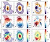 |
Fig. 7. Fitting results from 3DBAROLO with parameters set as described in Sect. 3.4. For all rows, the first column shows the data, the second the model, and the third the residual (data minus model). The first row shows the moment-0 emission (intensity), the second the velocity field (rotational velocity, Vrot), and the third the velocity dispersion (σ). The final 3DBAROLO ring is shown as the black ellipse and regions outside this ellipse are made semi-transparent to emphasize the region used for fitting. The major axis is shown in the first two rows by the dashed grey line. The kinematic center is shown by the green line in the first two columns of the second row. The approximate beam, assuming a static magnification factor across the image, is shown in the bottom-left of each image. |
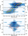 |
Fig. 8. PV diagrams from 3DBAROLO, upper: major axis, lower: minor axis. The blue contours show the contours of the data at 2, 3, 4, 5σ levels, and the red contours show the best-fit model to the data. In the major axis pv diagram, the yellow dots show the best fit rotational velocity in each of the rings. The right axis (VLOS) shows the velocities centered around the systemic velocity of the galaxy at the redshift of G09v1.97 (z = 3.63). The left axis (ΔVLOS) shows the velocities centered around the user-set systemic velocity, here 120 km/s (Table 5). |
Best-fit parametric from 3DBAROLO fitting.
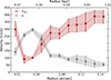 |
Fig. 9. Rotational velocity and dispersion as a function of radius for G09v1.97 for each ring in our 3DBAROLO fit. Red shows the rotational velocity and gray shows the dispersion. The errors are represented by the shaded regions for both. |
We plot Vrot and σ in each ring with increasing radius in Fig. 9. Excluding the innermost ring, Vrot rises steadily, and σ falls with increasing distance from the center of the galaxy, as expected for a rotating disk. Apart from this innermost ring, the decrease in σ with increasing radius is expected as the most turbulent motions mostly occur in the innermost regions of the galaxy (e.g., Fraternali et al. 2002; Boomsma et al. 2008; Tamburro et al. 2009; Sharda et al. 2019; Rizzo et al. 2023). The innermost ring exhibits what appears to be a ‘bump’ in Vrot and has a correspondingly lower σ value. This bump was also present in the fit where all parameters were left free and is significant (i.e., cannot be explained as an error). This elevated Vrot and lower σ could be indicative of an additional galaxy component such as a bar or a bulge (e.g., Amvrosiadis et al. 2025; Rowland et al. 2024). However, the elevated Vrot at the innermost ring does not appear as strong in the blue velocity portion major axis pv-diagram (Fig. 8), so it is possible that this is an asymmetric component in the galaxy, further discussed in Sect. 4.2. The corresponding increase in σ in the innermost ring is likely due to the strong emission in the eastern part of the dispersion map and dispersion residual (Fig. 7) and is likely dominating 3DBAROLO’s fitting procedure for the innermost ring. Given the limitations of the data and the inherent errors associated with both the lensing analysis and the kinematic modeling, we cannot make any conclusive statements about the cause of this bump.
The best-fit systemic velocity of the CO(6−5) emission from the kinematic fitting, Vsys = 109 km/s, corresponds to a redshift of z = 3.6300017, slightly higher than previously reported. This offset lies closer to the peak in the red portion of the spectrum, which occurs at 210 km/s in the image plane; see Fig. 2. This velocity offset from 0 is further discussed in Sects. 4.1.1 and 4.2.
Figure 7 shows an apparent offset in the kinematic center between the observed data and the model. We find a slight residual in the moment-0 map and in approximately the direction of the minor axis in the moment-1 map; see Fig. 7. Additionally, there is a residual in the velocity dispersion in the region corresponding to the residual in the moment-1 map. We further discuss these residuals in Sect. 4.2.
We note that although we assumed a static beam across the image (see Sect. 3.3.3), as has been done in previous kinematic studies of lensed galaxies (e.g., Amvrosiadis et al. 2025), the magnification across the image is not, in fact, static; this is easily seen in the differing sizes of the Voronoi cells in Fig. 6. In effect, the beam size should vary across the image, becoming larger in less magnified regions and vice versa in more magnified regions. The effect of this variation has been shown in previous studies (e.g., Dye et al. 2022), but remains difficult to quantify in the case of G09v1.974. This assumption primarily affects the number of rings used in the 3DBAROLO modeling, which is largely a user-defined preference.
We performed a simple investigation into the impact of the assumed static beam on our kinematic modeling results by varying the ring separation used in the 3DBAROLO modeling. We vary the separation from  (θmaj/5, corresponding to 23 rings) to
  (θmaj * 1.2, corresponding to 4 rings) in steps of a factor of two. We followed the same fitting procedure as described in Sect. 7. Through this investigation we found that the ring separation has a minimal impact on the results obtained for the fit. Figure C.1 shows the rotation curve and dispersion in each ring for the different ring separations and clearly shows that the variation of the number of used rings largely does not affect the shape of the curves and, thereby, the results of the kinematic modeling. We note that when using either four or five rings, we did not find the increase in rotational velocity or a corresponding decrease in dispersion found towards the center of the galaxy. We suggest that the feature in the center of the galaxy producing the increase is seen when using a higher number of rings and smoothed out if using an insufficient number of rings; however, we acknowledge that with the current data, it is difficult to determine the nature of this feature. We found that the
  varied between 2.6 − 3.5 with an average value of 3.2 ± 0.15. Given that the average value found in this investigation was is within errors of our initial fit using 11 rings, we conclude that the size of the beam, and thereby the assumed ring separation, does not largely affect the results of this work.
4. Discussion
4.1. G09v1.97 in the source plane
4.1.1. Spectral line shapes
Motivated by the clear velocity gradient seen in the source-plane reconstruction moment-1 map (Fig. B.2), we created channel maps across the reconstructed cube in 50 km/s bins. We masked these images to only show emission at locations above 5σ in the moment-0 map (i.e., emission in the region shown in the masked Voronoi moment-0 map shown in Fig. B.2); see Fig. 10. These channel maps clearly indicate a south-north velocity gradient across the line profile, possibly providing another indication of rotation. However, this could also be an indication of merger activity (e.g., Yang et al. 2019).
We investigate the emission line profiles, which are of particular interest given their asymmetric profiles. Yang et al. (2019) clearly demonstrated that there is differential magnification occurring across the emission line. This is also clear from the velocity maps (Fig. 10) as the emission in redder velocities is shifted north towards the caustic line, meaning that the magnification will be higher in that region of the spectrum. We investigate this through two different, respective, methodologies for the H2O and the CO(6−5) emission. In the case of the CO(6−5) emission, we used the source plane cube as described in Sect. 3.3.3. Since we did not create a source plane H2O spectral cube, we neede to investigate the emission line profile by parametrically modeling the red and blue portions of the emission line, as described below.
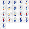 |
Fig. 10. Source plane channel maps for the CO(6−5) emission from the demagnified source plane emission cube described in Sect. 3.3.3. The velocities covered by each bin are shown at the top of the image. The background mesh shows the Voronoi mesh pixels prior to interpolation to a square grid. Black line shows the caustic line. A clear velocity gradient is evident across the emission line. |
We show the approximate source plane spectrum for the CO(6−5) emission in Fig. 11. Although units in the source plane reconstructions from PYAUTOLENS are arbitrary, qualitative investigations between source plane and image plane spectra can be performed by normalizing both spectra before comparison. We only reconstructed the channels with the brightest emission and, therefore, do not have a full spectrum across all velocities in the source plane. Further, note that both the image and source plane spectrum are normalized per-channel sums of the flux inside a region, and therefore, figures depicting the image-plane CO(6−5) spectrum in units of mJy may appear slightly different. The region used for the spectral extraction of the normalized image plane spectrum is the same as used previously to extract the source plane spectra for H2O and CO(6−5) as well as for extracting the underlying dust continuum (see Sect. 3) and is shown in Fig. 1. The region used to extract the source plane spectrum was the same region used in the 3DBAROLO modeling, shown by the black ellipse in Figs. 7 and 11. In addition, we extracted the source plane spectrum from a northern and southern region G09v1.97, corresponding to above/inside the caustic line and below the caustic line. We calculated the RMS in each channel using the same simple sampling method as described in Sect. 3.2.
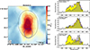 |
Fig. 11. Comparison between the approximate image plane spectrum and source plane spectrum of the CO(6−5) emission in G09v1.97. Left: Source plane moment-0 map of the CO(6−5) emission with the different regions used for the source plane spectral extraction. Right: Normalized source plane spectrum (in yellow) compared to the normalized image plane spectrum (in grey) extracted from the region used in 3DBAROLO modeling (top), a northern region of the source located inside the caustic line (middle), and a southern region of the source located outside the caustic line (bottom). Note: the per-channel values are the normalized sum in a specific region as described in Sect. 4.1.1 and not a standard flux. The error bars are shown for each channel. Single Gaussian profiles are shown in red, while double Gaussian profiles are shown in blue. |
We found that the source plane CO(6−5) spectrum from the 3DBAROLO region was significantly flatter than the image-plane spectrum and does not appear to have two clear red and blue components, as seen in the image plane spectrum. Instead, we find a profile that is more similar to a double-horned profile, indicative of rotation, and in good agreement with our results from 3DBAROLO. We investigated the systemic velocity offset of 109 km/s from the 3DBAROLO modeling by fitting the source plane spectrum with a single Gaussian profile and using two Gaussian profiles. We find that the systemic velocity in the source plane spectrum is 68 ± 29 km/s using a single Gaussian profile and that the red component peaks at 186 ± 18 when using two Gaussian profiles. This does not fully account for the offset in the systemic velocity in the 3DBAROLO modeling but provides an indication that the cause of this offset may be the asymmetric line profile.
We further investigated the two components seen in the image plane spectrum by considering the spectrum extracted from the northern and southern regions. It is clear that the red peak in the spectrum corresponds to emission in the north of the image and the blue peak in the spectrum to emission in the south of the image; see Fig. 11. The red region is located within the caustic lines and therefore subject to higher magnification than the blue region, which accounts for the discrepancy in the peak of the components in the image plane spectrum; see the bottom- right panels in Fig. 11. However, the source plane spectrum from the entire source (i.e., encompassed in the region used for 3DBAROLO region) still appears to be brighter in redder regions of the spectrum. This could be a residual effect of the lens modeling or an observational effect caused by, for example, inclination effects. Kohandel et al. (2019) shows that a change in inclination can have unexpected and asymmetric effects on the line profile when the source is not an ideal disk. Future observations and source plane analysis of additional bright, atomic, or molecular emission lines such as [C II] could assist in determining the cause of the asymmetric source plane line profile.
We now consider the line profile of the H2O emission. We divided the H2O lines into two bins, with each bin covering one of the two respective peaks in the spectrum of both molecules; these bins covered the velocity ranges of −300 to 175 km/s, corresponding to the peak in the blue region of the spectrum, and 175 to 500 km/s, corresponding to the peak in the red region of the spectrum. We found that the magnification factor is different in the red and blue regions of the spectrum with μblue = 8.87 and μred = 13.97, making the ratio of the emission, as described in Sect. 3.2.2, peakred/peakblue ≈ 1.5. Both the observed and corrected H2O ratios are lower than those found for the CO(6−5) emission, while the magnification factor in the blue part of the spectrum remains approximately constant between the two lines. This suggests that the majority of the differential lensing is occurring in redder portions of both spectra.
An alternative explanation for the differences in the peak strengths of the emission lines is an inclination effect. 3DBAROLO fitting results suggest that G09v1.97 lies at an inclination of i ≈ 50°. At this inclination, an asymmetric double-horned profile would be expected (e.g., Yttergren et al., in prep.). However, if this profile is consistent with rotation or interactions, it is unclear from the spectra alone (e.g., Rizzo et al. 2022). The spectrum of the CO(6−5) in the image plane is qualitatively similar to that of one component of the merger SMG HXMM01, while the source plane spectrum qualitatively resembles another component (Xue et al. 2018). Without additional observations, it is difficult to come to robust conclusions about the source of the asymmetric line profile.
4.1.2. Emission morphology and extent
We investigated G09v1.97 in the source plane primarily using the nonparametric source-plane reconstruction images, as described in Sect. 3.3.3. We did not include the H2O+ emission in this analysis due to the significantly lower angular resolution, which does not allow for a robust comparison. We opted to exclude the parametric source models from this investigation due to the a priori source morphology assumptions inherent to these models. We show the spatial extent of the continuum emission, CO(6−5), and H2O emission from the nonparametric source reconstruction of the emission (see Sect. 3.3.2) in Fig. 12. Rather than showing σ level contours, we show the contours at percentage levels (30%, 40%, 60%, 80%, and 100%) of the peak flux for the specific tracer with darker colors corresponding to higher percentages. We opt to show the extent in this manner due to the uncertainties in the lens modeling towards the edges of emission regions where the flux levels are lower. We primarily focus on the regions where the flux is at least 50% of the maximum value for that emission type. In addition, we show the enclosed flux in circular apertures increasing as a function of the beam size out to 80% of the total flux in the image. The noise in the image was sampled, similarly to the sampling performed for the spectra (see Sect. 3), corresponding to the size of the aperture.
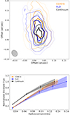 |
Fig. 12. Top: Source plane contour plots of the dust continuum, CO(6−5), and H2O emission in G09v1.97. The contours are at 30, 40, 60, 80, 100% levels of the maximum value of the individual tracer. The approximate beam, assuming a static magnification factor across the image, is shown in the bottom- left of the image. Bottom: Normalized enclosed flux in circular apertures increasing from the center of the CO(6−5), dust continuum, and H2O emission out to 80% of the total flux of the image. It is clear that the dust continuum emission is the most compact of the emission types, whereas the CO(6−5) and H2O emission closely match in emission extent. |
The dust continuum emission seems to be the most compact of the three tracers. We find that the distribution of the H2O and the CO(6−5) are very similar, with CO(6−5) exhibiting a slightly larger extent. CO(6−5) and H2O emission have previously been found to be correlated with regions of star formation within the galaxy (Greve et al. 2014; Liu et al. 2015; Yang et al. 2013, 2016; Omont et al. 2013; Jarugula et al. 2021; Pensabene et al. 2022), and therefore, their extents should be similar (e.g., Quinatoa et al. 2024). However, the H2O emission is expected to be produced in part by IR pumping (e.g., González-Alfonso et al. 2010, 2014, 2022) and is correlated with warm dust (Tdust ≈ 40 − 70 K Liu et al. 2015). Therefore, it is interesting that the continuum appears more compact than the H2O emission. However, a significant fraction of the H2O emission can originate from collisional excitation (e.g., Yang et al. 2013, 2019; González-Alfonso et al. 2022; Liu et al. 2017). In addition, even assuming that the bulk of the dust and H2O are physically distributed in the same region of the galaxy, the scale of the dust emission will appear smaller due to a temperature gradient. The larger spatial extents of the molecular gas compared to that of the dust continuum emission has previously been seen in studies of z ≈ 2 − 3 SMGs (e.g., Fu et al. 2012) with the proposed explanation of temperature and optical depth gradients (e.g., Calistro Rivera et al. 2018), which could indeed also be the case for G09v1.97. Overall, the distribution of the CO(6−5) emission closely matches that of the H2O while the continuum appears more compact. The H2O emission map in this paper is the highest angular resolution map to date at such a high redshift. We further note that the exact distribution of the different emission types is, in part, governed by the regularization coefficient described in Sect. 3.3.2, particularly with regard to the apparent smoothness of emission.
4.1.3. Lensing comparison to Yang et al. (2019)
Here, we further investigate the discrepancies between the lens modeling results between our analysis and Yang et al. (2019). As mentioned previously, Yang et al. (2019) found that the best-fit lens model of G09v1.97 required two parametric Sérsic sources. The authors postulated that the two peaks in the CO(6−5) (and other molecular line emission) corresponded to two different galaxies that were undergoing a merger or interaction. In this work, a single source was sufficient to produce successful lens modeling results for both the parametric and nonparametric source modeling performed. Of particular interest are the nonparametric models, which do not require morphological assumptions, but these models also do not provide any indication of two sources in the source plane (see Fig. 6).
To better compare our results to those of Yang et al. (2019) for the CO(6−5) emission, we performed nonparametric source reconstructions on the two peaks seen in the CO(6−5) spectrum. We used the two bins described in Sect. 4.1.1 covering velocities between −300 to 125 km/s and 125 to 500 km/s. These ranges correspond approximately to the blue and red components described in Yang et al. (2019)5. We used the same procedure as described in Sect. 3.3.2 to perform the nonparametric lensing.
We find that when the spectrum is broken into these two bins, there does indeed appear to be a southern component corresponding to the blue peak of the CO(6−5) emission and a northern component corresponding to the red peak of the CO(6−5) emission. However, unlike in Yang et al. (2019), these two components are co-spatial around the caustic line, meaning that they do not fully appear as separate sources. We show the images, models, and residuals for all modeled emission in Fig. B.1. We suggest that the primary reason for the discrepancy between our modeling results and those from Yang et al. (2019) is due to the velocity gradient seen in the demagnified CO(6−5) source plane emission cube channel maps (Fig. 10). Without the additional per-channel information available in the source plane, the results of the two-bin model could easily be interpreted as two separate sources. This highlights the importance of creating source plane emission cubes during the lens modeling process.
4.2. G09v1.97: Merger or disk
Studies in recent years have extended the redshift range of kinematic fitting significantly (e.g., Smit et al. 2018; Rizzo et al. 2020; Fujimoto et al. 2025; Rowland et al. 2024). This has led to further progress in understanding the kinematics of high-redshift massive galaxies. With regard to G09v1.97 and other DSFG/SMG galaxies, one of the primary motivations of kinematic studies is establishing whether DSFG/SMGs are largely merging or post-merger galaxies as they are often likened to ultraluminous IR galaxies (ULIRGs Sanders & Mirabel 1996) in the local universe due to their many shared properties (e.g., Tacconi et al. 2008; Engel et al. 2010; Riechers et al. 2011; Bothwell et al. 2013), which are primarily either undergoing or have recently undergone mergers (e.g., Kim et al. 2002; Veilleux et al. 2002). However, it has been shown that accurately distinguishing between mergers and disk galaxies at high redshift is very difficult, primarily for reasons relating to angular resolution and sensitivity challenges (Rizzo et al. 2022; Peng et al. 2023; Cathey et al. 2024). Although observations of gravitationally lensed galaxies typically have higher angular resolution and sensitivity due to the magnification effects of the lensing phenomenon, they also provide challenges in accurately determining the source plane properties of the lensed galaxy (e.g., Dye et al. 2014; Yang et al. 2019; Rybak et al. 2020). For example, Rizzo et al. (2022) simulated galaxies at high, mid, and low angular resolutions and demonstrated the difficulties in accurately distinguishing between disks versus mergers. Below, we discuss the characteristics of G09v1.97 and attempt to classify the source as either a merger or a disk. Further, we examine some of the limitations caused by the gravitational lens modeling.
We report  for G09v1.97, which suggests that the source is dominated by ordered motion rather than turbulence. We compare the Vmax/σ value found for G09v1.97 to other galaxies across a wide redshift range in Fig. 14. We find that G09v1.97 has a lower V/σ value than has been found for other sources at comparable redshifts (e.g., Hodge et al. 2012; Rizzo et al. 2023; Amvrosiadis et al. 2025) and instead lies closer to the turbulent disks found at comparable and higher redshifts (e.g., Turner et al. 2017; Parlanti et al. 2023). However, there are a number of important caveats to note when using this comparison sample. The first is the choice of a gas tracer. CO(6−5) emission traces warmer and denser gas than [C II] (Carilli & Walter 2013). The samples that use CO emission are limited to lower-J transitions and, therefore, trace colder and more diffuse gas than the CO(6−5) emission used in this work. Secondly, the V/σ values used in different studies are calculated differently. Some studies use
  , as is used in this paper, while others use rotational velocities extracted at, for example, re. Thirdly, there is a wide variety of data quality used for calculating the V/σ values plotted in the figure. Finally, Hα is known to exhibit systematic differences in V/σ compared to those found for [C II] and CO emission in the same galaxy (Rizzo et al. 2024). However, we argue this sample still provides a relevant and meaningful basis for comparison.
Rizzo et al. (2022) present a method called PVSPLIT that shows promise as a tool able to separate between disks and mergers. This method relies on three parameters, Pmajor, PV, and PR, obtained from the PV major axis diagram. The PVSPLIT method has been further investigated by Roman-Oliveira et al. (2023) with a sample of mergers and disk galaxies from ALMA mock observations of SERRA simulated (Pallottini et al. 2022) galaxies together with a random selection of 9 local WHISP (van der Hulst et al. 2001) survey disk galaxies. From this Roman-Oliveira et al. (2023) suggested a plane dividing disks from mergers following the equation: −0.63Pmajor − 0.27PV + 2.78PR − 2.72 = 0. PVSPLIT is a promising method, but has only been tested on a very limited sample without galaxies with known outflows. Nonetheless, we calculate the PVSPLIT parameters for G09v1.97 and find: Pmajor = −1.56, PV = −0.33, and PR = 0.50. Using the dividing line suggested by Roman-Oliveira et al. (2023), this places G09v1.97 on the side of mergers, albeit close to the dividing plane. The distance between G09v1.97 and the dividing plane is very small, only 0.08. This suggests that G09v1.97 may be a merger, but it may also be one of the sources subject to scattering around the dividing plane or this may be the region of the Pmajor − PV − PR parameter space where disks with outflows, or late stage minor mergers, will populate when they have been placed into the PVSPLIT scheme as the tool is tested on additional sources.
Using the classification scheme from Kohandel et al. (2024) for [C II] emission, G09v1.97 would be classified as a warm rotating disk. However, this classification scheme was developed for [C II] and Hα emission, and therefore, extrapolating to CO(6−5) emission could skew the interpretation of the Vmax/σ value. Both [C II] and CO(6−5) emission are thought to trace molecular gas, with [C II] likely tracing more extended emission (e.g., Carilli & Walter 2013).
It could be the case that the CO(6−5) emission has a higher dispersion value (σ) value since it is tracer warmer and therefore more turbulent gas, and thereby a lower Vmax/σ value (under the assumption that we are probing Vmax with the current data). On the other hand, we are likely not tracing the Vmax for the entire galaxy with such a warm gas tracer, and therefore even if the dispersion value turns out to be higher in CO(6−5) than other, colder gas tracers, the overall Vmax/σ ratio may remain unchanged. Additionally, observations of colder gas tracers that probe further into the disk may exhibit a smaller ratio due to larger Vmax values and a lower average dispersion. To verify which of these scenarios is occurring, a kinematic analysis would need to be performed on, for example, very high angular resolution observations of [C II] emission in G09v1.97.
We find that G09v1.97 also follows the classification scheme for a rotating disk used by Rizzo et al. (2022). In this scheme, to be classified as a rotating disk, the galaxy must have V/σ > 1.8 to maintain sufficient rotational support over the turbulence (e.g., Wisnioski et al. 2015, 2019). Additionally, the galaxy must exhibit a smooth velocity gradient in the moment-1 map. G09v1.97 fulfills both of these criteria. Similar criteria are commonly employed across a wide redshift range (e.g., Förster Schreiber et al. 2009; Wisnioski et al. 2015; Smit et al. 2018; Bakx et al. 2020; Rizzo et al. 2022).
We now turn to investigating the residuals found in the moment maps from our best-fit 3DBAROLO modeling. Figure 13 shows the zoomed-in moment-1 residual with a different colorscale and with the Voronoi grid along with the S/N map from the lens modeling as described in Sect. 3.3.3. We first note that the largest of these residuals in both the moment-0 and moment-1 maps are located outside of the region used for fitting in the 3DBAROLO models, meaning that the  ratio found for G09v1.97 is not affected by these residuals. Here we investigate different possibilities, primarily relating to the residuals inside this fitting ellipse where the significance of the emission is higher when considering the source plane error maps, to explain these residuals. We investigated the possibility that the residuals were caused by the interpolation from a Voronoi mesh onto a square pixel grid. We returned to the creation of the CO(6−5) source plane emission cube, described in detail in Sect. 3.3.3, and verify that the residuals are not caused by this interpolation through two methods. In the first, we used twice the number of pixels in the Voronoi mesh prior to interpolation to a square grid, and in the second, we used a rectangular mesh instead of a Voronoi mesh. In both cases, we found very similar residuals, suggesting that the interpolation from the Voronoi mesh to the square pixel grid was not the cause of the residuals. There does not appear to be a correlation between regions of high errors in the source plane error map (see Fig. B.3) and the strongest velocity residuals. We therefore conclude that there is no indication that the residuals result from a poorly fitting lens mass model. For the remainder of this paper, we consider only the residuals inside the region used for 3DBAROLO fitting, shown by the white ellipse in Fig. 13, due to the low S/N of regions outside this ellipse.
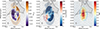 |
Fig. 13. Residual moment-0 and moment-1 maps from 3DBAROLO fitting and the S/N map of the emission using the source plane error map (i.e., source plane intensity/moment-0 divided by the source plane intensity error map) as described in Sect. 3.3.3. Note: the first two panels are a zoomed-in version of the same images shown as in Fig. 7 (rows 1 and 2, column 3), but with a different color scale. The grey grid shows the Voronoi pixels prior to interpolation to the square pixel grid, as described in Sect. 3.3.3. The black line shows the caustic line and the white ellipse shows the region used for 3DBAROLO fitting (i.e., the final ring). As in Fig. 7, any emission outside the fitting region is semi-transparent. The approximate beam, assuming a static magnification factor across the image, is shown in the bottom- left of the image. |
Under the assumption that these features are not caused by the lens modeling, they could instead be indicative of noncircular motions in G09v1.97. First, we consider the significance of the moment-1 residuals. We calculated the significance of the velocity residuals by considering the moment-0 emission in regions where the moment-1 residuals exceed 125 km/s (within the fitting region used by 3DBAROLO) by taking the ratio of the moment-0 flux to total error as a proxy for their significance. We note that the independent resolution element, i.e. the assumed source plane beam area, is propagated into the measurement by calculating the total area of pixels with velocity > 125 km/s in the fitting region. These residuals are statistically significant (∼6σ), and we therefore turn to investigating their nature and discussing possible physical interpretations.
One possibility to explain this emission is a biconical outflow approximately perpendicular to the major axis of the galaxy. In this scenario, the relative lack of a clear blue component could be explained by either interactions from this outflowing emission with the disk or simply an obscuration effect from the disk. We find no clear evidence of outflows in the CO(6−5) emission spectrum; however, the complex line profiles do not allow for a clear exclusion of this feature. Observations of specific outflow tracers (e.g., OH+) could help to establish if this explanation for the residual is correct.
Another explanation could be that of an additional galaxy located behind G09v1.97 at spatial offsets of > 100 km/s6. However, we find no clear signs of merger activity that would be expected from such a nearby companion galaxy and would expect a lower  ratio in the case of an on-going merger or interaction. Previous studies have shown some evidence of flattening rotation curves with V/σ > 2 while also exhibiting evidence of interactions and mergers (e.g., Xue et al. 2018). In the case of G09v1.97, should a background galaxy be present, it would be expected that the residual intensity map would show elevated values at the same spatial extents. We do find a residual in the moment-0 residual map from 3DBAROLO (Fig. 13) that is slightly offset from the moment-1 residual, which could be interpreted as an additional source of emission. A similar (and possibly more likely) scenario is that of a tidal tail as a remnant of a merger or interaction. Given that G09v1.97 appears to be more consistent with a warmer rotating disk than a fully settled, cold, rotating disk, this could explain the higher dispersion occurring in G09v1.97. This is further discussed in Sect. 4.3.
One final possibility for this residual is a bar, as has been suggested for similar residuals (e.g., Amvrosiadis et al. 2025). This could explain the features in the major axis pv-diagram (Fig. 8) and the bump in the Vrot and σ at the innermost radii (Fig. 14). However, the lack of a clear blue component in the moment-1 residual and the location of the moment-0 residual raise doubts about this possibility.
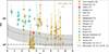 |
Fig. 14. Evolution of V/σ with redshift for G09v1.97 (shown by the pink star) and literature sources. The literature sample is taken from Amvrosiadis et al. (2025), Roman-Oliveira et al. (2023), Hodge et al. (2012), Fraternali et al. (2021), Lelli et al. (2023), Liu et al. (2023), Neeleman et al. (2023), Parlanti et al. (2023), Posses et al. (2023), Rizzo et al. (2020, 2021, 2023), Rowland et al. (2024), Turner et al. (2017). For the literature sample, we show atomic tracers (in this case [C II], [O III], Hα emission) in yellow and molecular gas tracers (in this case, different CO transitions) in blue. We show the semi-analytic model from Wisnioski et al. (2015) in gray with Q values ranging between 0.67 to 2 and the fiducial model of Q = 1 in the dashed gray line. |
Although these velocity residuals are statistically significant and indicative of noncircular motion in G09v1.97, their physical origin is not yet understood. Overall, we find that the results of the performed kinematic modeling are most consistent with G09v1.97 being a warm rotating disk, and suggest that the residual is likely some additional component to the galaxy, such as a tidal tail.
4.3. Physical properties of the warm rotating disk G09v1.97
G09v1.97 has previously been shown to be one of the most luminous dusty star-forming galaxies in the high-redshift universe with a total IR luminosity of LIR = (1.4 ± 0.7)×1013 L⊙ (Yang et al. 2019). Assuming a Chabrier initial mass function (IMF; Chabrier 2003) and the relation between SFR and LIR as SFR ∼ 10−10LIR[L⊙], this implies a SFR of 1400 ± 700 M⊙ yr−1. Fitting the CO(6−5) emission in the source plane, we find a spatial extent of  , corresponding to 1.5 kpc × 0.88 kpc at z = 3.63. This implies a surface star formation rate density of ΣSFR ≈ 340 M⊙ yr−1 kpc−2.
Following Wang et al. (2013), Venemans et al. (2016), and Yang et al. (2017), we calculate the dynamical mass of G09v1.97 assuming that the system is a rotating disk using the following,
![Mathematical equation: $$ \begin{aligned} M_{\mathrm{dyn} } = (2.35 \times 10^5) \left(\frac{V_{\mathrm{c} }}{\mathrm{km\,s^{-1}}}\right) \left(\frac{r}{\mathrm{kpc}}\right) [\mathrm{M}_{\odot }], \end{aligned} $$](/articles/aa/full_html/2026/03/aa51460-24/aa51460-24-eq62.gif) (2)
(2)
where Vc is the rotational velocity at radius r. We consider the radius and rotational velocity in the outermost ring from 3DBAROLO, corresponding to Vc = 386 km/s and r = 1.07 kpc, resulting in Mdyn = (3.7 ± 0.1)×1010 M⊙7. This is in good agreement with the dynamical mass found in Yang et al. (2017) for G09v1.97.
We estimate the gas mass fraction by first calculating the gas mass from the CO(6−5) emission. We use the conversion ratio between the CO(6−5) and CO(1−0) emission based on single component large velocity gradient (LVG) modeling of the observed CO spectral line energy distribution (SLED) performed in Yang et al. (2017), wherein the ratio is very similar to LVG modeling of z ≈ 2 galaxies using two-component CO SLEDs (Boogaard et al. 2020). This conversion assumes that the CO(6−5) and CO(1−0) emission come from the same spatial region, which is unlikely to be the case; however, it is the best approximation with the given data. We further note that, although conversions from higher-J transitions to CO(1−0) are commonly performed in high-redshift studies, where obtaining CO(1−0) observations can be difficult, this conversion is inherently uncertain and, therefore, the gas mass obtained here should be seen as an estimate. Assuming αCO = 0.8 (a typical value used for local ULIRGS Downes & Solomon 1998) and a helium contribution of 36% (Yang et al. 2017), we obtained a gas mass in the region of CO(6−5) emission of Mgas = (1.8 ± 0.74)×1010 M⊙. We note that the value chosen for αCO can strongly impact the gas mass estimate (see e.g., Dye et al. 2022) as this value can range from αCO = 0.8 − 4.0; therefore, we incorporated a larger error on the gas mass (approximately a factor 4) to represent this range. This implies a depletion time (defined as tdep = Mgas/SFR) for G09v1.97 of 13 ± 8 Myr, lower than the value found for G09v1.97 by Yang et al. (2017) but within the error range. Similarly, this value is lower, but within errors, than the depletion time that has been found for other strongly lensed SMGs at similar redshifts (e.g., Yang et al. 2017). This implies a gas mass fraction (Mgas/Mdyn) of 0.5 ± 0.02, lower than reported in Yang et al. (2017) but still within an expected range for strongly lensed SMGs (e.g., Yang et al. 2017).
One possibility to explain such a high SFR is that the IR luminosity could be contaminated by the presence of an AGN. However, Yang et al. (2019, 2020) argue that there is no clear evidence of an obscured AGN at the center of G09v1.97; this is supported by G09v1.97’s similar line-to-IR luminosity ratio for both CO(6−5) and H2O as well as the q parameter (Condon 1992) as discussed in Yang et al. (2016, 2020). The surface brightness distribution of the CO(6−5) emission (as shown by, e.g., kinematic modeling) does not reveal an additional compact, bright, central component in the residual intensity map (see Fig. 7). Such a feature, if present, could have been indicative of AGN activity. In addition, we do not observe any excess emission appearing as a bright central source in either the H2O or continuum maps. Hence, we find no evidence of an AGN in the observed frequencies. Should there be an AGN affecting the LIR and thereby SFR, an alternative method to determine the SFR is through the use of the CO(6−5) emission given that mid-J CO emission is thought to trace star-forming regions of the galaxy (e.g., Greve et al. 2014; Lu et al. 2015). Through this method, and assuming that the CO(6−5) and CO(7−6) emission are very similar, a reasonable estimate based on CO SLED modeling from Yang et al. (2017), we obtain SFRCO ≈ (2515 ± 260) M⊙ yr−1 using the conversion between CO(7−6) and SFR given in Lu et al. (2015), implying a two times smaller depletion time. Thus, we return to the question of how such a high SFR could be triggered.
Contrary to what was found by Yang et al. (2019), we find no clear evidence of merger activity in G09v1.97 and instead have demonstrated through kinematic modeling that G09v1.97 appears to be a warm rotating disk. However, we also find evidence in the residuals from 3DBAROLO modeling for an additional component such as a tidal tail or additional galaxy. In the former, G09v1.97, observed at its present epoch, is a post-merger coalescence galaxy that has relatively recently settled into a rotating disk. In the latter, given the close velocity separation between the additional component and G09v1.97, the additional component would be interpreted as an interaction. In both scenarios, the SFR of the galaxy is expected to increase due to the compression of the gas from ongoing or previous interactions. This is a similar finding to the results reported by Kade et al. (2024) and consistent with the commonly accepted theoretical paradigm of massive galaxy evolution (e.g., Hopkins et al. 2008).
5. Conclusions
We report high-resolution ALMA observations of CO(6−5), H2O(211 − 202), and the underlying dust continuum emission in the z = 3.63 gravitationally lensed object DSFG G09v1.97. We performed parametric and nonparametric source reconstructions of the different detected emission using the sophisticated, publicly available lens modeling code PYAUTOLENS (Nightingale et al. 2021). We performed source-plane kinematic modeling of the CO(6−5) emission using 3DBAROLO. Our conclusions are presented below.
-
We further improved the lensing model of G09v1.97 using the high-resolution dust continuum emission and applied this lens model to the line emission. The magnification factors from our lens model are in good agreement with those from Yang et al. (2019).
-
We used a nonparametric pixelated modeling of the CO(6−5) emission to create a source-plane emission line cube. We find no evidence that the CO(6−5) emission requires two sources to successfully model G09v1.97. Instead, we find a single source exhibiting a smooth velocity gradient across the CO(6−5) source-plane emission line cube. We suggest that the discrepancy between the results provided in Yang et al. (2019) and what has been found in this work stems primarily from the velocity gradient found in the source plane. Without creating a demagnified source plane emission cube, it is challenging to properly interpret the emission.
-
We compared the extent of the dust continuum, CO(6−5), and H2O emission in the source plane, finding that the dust continuum emission is the most compact of the three emission types. Although H2O emission is typically correlated with dust emission due to IR pumping, it appears more extended than the dust continuum in this work.
-
We performed a kinematic modeling on the source-plane CO(6−5) emission line cube using 3DBAROLO and find that the kinematics are well explained as a rotating disk with a maximum rotational velocity of
 km/s and an average dispersion of
  km/s, implying Vmax/σ = 2.8 ± 0.4. Therefore, ordered rotation dominates over turbulence in G09v1.97.
 -
We compared the V/σ value found for G09v1.97 with a representative comparison sample between 1 < z < 8 and find that G09v1.97 lies within predicted values from semi-analytic models but seems to exhibit relatively more turbulence than other disk galaxies at similar redshifts. According to a classification scheme developed from Kohandel et al. (2024), G09v1.97 should be classified as a warm disk. Alternatively, the in-development tool PVSPLIT provides an indication that G09v1.97 is undergoing a merger event.
-
We found evidence of noncircular motions in the velocity and dispersion residuals from the kinematic fitting. Similarly, we find evidence of a residual in the moment-0 map. These residuals cannot be explained by the lensing analysis and source plane cube reconstruction and are statistically significant (∼6σ). We therefore suggest that these residuals represent an additional component, such as a biconical outflow, tidal tail, or additional background galaxy.
-
We calculated the dynamical mass of G09v1.97 using the rotational velocity in the final ring from 3DBAROLO as a proxy for the turnover radius. We find that, within 1 kpc, the dynamical mass of G09v1.97 is Mdyn = (3.7 ± 0.1)×1010 M⊙. Furthermore, we calculated the gas mass and SFR from both the IR luminosity and CO emission; we find Mgas = (1.8 ± 0.74)×1010 M⊙, SFRLIR = (1400 ± 700) M⊙ yr−1, and SFRCO ≈ (2515 ± 260) M⊙ yr−1. Together, these values imply a very low depletion time (13 ± 8 Myr) in comparison to other galaxies at similar redshifts.
We suggest that G09v1.97 has either recently undergone or is currently undergoing an interaction or merger event, causing the residuals seen in the moment-1 emission from the 3DBAROLO modeling. Combined with the high SFR and a low depletion time, we suggest that the interaction triggered extreme star formation. In this scenario, G09v1.97 has recently settled into a turbulent, rotating disk that is rapidly consuming its gas and showing non-disk morphological features due to likely recent or on-going interactions or merger events.
Observations of a colder gas tracer, such as [C II], using similar or higher angular resolution observations, could help probe further into the disk of G09v1.97 and provide additional clues to the ongoing dynamical processes in the galaxy. Furthermore, observations of specific outflow tracers, such as OH+, could assist in a more robust identification of the additional feature seen in the 3DBAROLO modeling, in particular, to determine whether it is a biconical outflow or possible tidal tail. G09v1.97 remains a remarkable target for future observational campaigns aimed at understanding the ISM and dynamics of galaxies at this epoch.
Acknowledgments
The authors thank the anonymous referee for their useful comments which improved the quality of the manuscript. The authors also thank Ian Smail and Hai Fu for useful comments that improved the manuscript. K.K. acknowledges support from the Nordic ALMA Regional Centre (ARC) node based at Onsala Space Observatory. The Nordic ARC node is funded through Swedish Research Council grant No. 2019-00208. M.Y. acknowledges support via research grants from the Knut and Alice Wallenberg Foundation. K.Kn. acknowledges support from the Swedish Research Council and the Knut and Alice Wallenberg Foundation. S.K. and C.Y. gratefully acknowledge funding from the European Research Council (ERC) under the European Union’s Horizon 2020 research and innovation programme (grant agreement No. 789410). SD acknowledges support from the Science and Technology Facilities Council (grant: ST/X000982/1). AC acknowledges support from NASA Astrophysics Data Program. E.I. gratefully acknowledges financial support from ANID – MILENIO – NCN2024_112 and ANID FONDECYT Regular 1221846. M.J.M. acknowledges the support of the National Science Centre, Poland through the SONATA BIS grant 2018/30/E/ST9/00208 and the Polish National Agency for Academic Exchange Bekker grant BPN/BEK/2022/1/00110. The National Radio Astronomy Observatory is a facility of the National Science Foundation operated under cooperative agreement by Associated Universities, Inc. This paper makes use of the following ALMA data: ADS/JAO.ALMA#2018.1.01710.S and ADS/JAO.ALMA#2015.1.01320.S. ALMA is a partnership of ESO (representing its member states), NSF (USA) and NINS (Japan), together with NRC (Canada), NSTC and ASIAA (Taiwan), and KASI (Republic of Korea), in cooperation with the Republic of Chile. The Joint ALMA Observatory is operated by ESO, AUI/NRAO and NAOJ.
References
- Amvrosiadis, A., Lange, S., Nightingale, J. W., et al. 2025, MNRAS, 537, 1163 [Google Scholar]
- Bakx, T. J. L. C., Tamura, Y., Hashimoto, T., et al. 2020, MNRAS, 493, 4294 [NASA ADS] [CrossRef] [Google Scholar]
- Barger, A. J., Cowie, L. L., Sanders, D. B., et al. 1998, Nature, 394, 248 [Google Scholar]
- Barger, A. J., Cowie, L. L., Chen, C. C., et al. 2014, ApJ, 784, 9 [NASA ADS] [CrossRef] [Google Scholar]
- Blain, A. W., Smail, I., Ivison, R. J., Kneib, J. P., & Frayer, D. T. 2002, Phys. Rep., 369, 111 [Google Scholar]
- Boogaard, L. A., van der Werf, P., Weiss, A., et al. 2020, ApJ, 902, 109 [NASA ADS] [CrossRef] [Google Scholar]
- Boomsma, R., Oosterloo, T. A., Fraternali, F., van der Hulst, J. M., & Sancisi, R. 2008, A&A, 490, 555 [NASA ADS] [CrossRef] [EDP Sciences] [Google Scholar]
- Bothwell, M. S., Smail, I., Chapman, S. C., et al. 2013, MNRAS, 429, 3047 [Google Scholar]
- Bussmann, R. S., Pérez-Fournon, I., Amber, S., et al. 2013, ApJ, 779, 25 [NASA ADS] [CrossRef] [Google Scholar]
- Calistro Rivera, G., Hodge, J. A., Smail, I., et al. 2018, ApJ, 863, 56 [Google Scholar]
- Cañameras, R., Yang, C., Nesvadba, N. P. H., et al. 2018, A&A, 620, A61 [Google Scholar]
- Cañameras, R., Nesvadba, N. P. H., Kneissl, R., et al. 2021, A&A, 645, A45 [EDP Sciences] [Google Scholar]
- Carilli, C. L., & Walter, F. 2013, ARA&A, 51, 105 [NASA ADS] [CrossRef] [Google Scholar]
- Casey, C. M., Narayanan, D., & Cooray, A. 2014, Phys. Rep., 541, 45 [Google Scholar]
- Cathey, J., Gonzalez, A. H., Lower, S., et al. 2024, ApJ, 967, 11 [NASA ADS] [CrossRef] [Google Scholar]
- Chabrier, G. 2003, PASP, 115, 763 [Google Scholar]
- Chapman, S. C., Blain, A. W., Smail, I., & Ivison, R. J. 2005, ApJ, 622, 772 [NASA ADS] [CrossRef] [Google Scholar]
- Condon, J. J. 1992, ARA&A, 30, 575 [Google Scholar]
- Danielson, A. L. R., Swinbank, A. M., Smail, I., et al. 2017, ApJ, 840, 78 [NASA ADS] [CrossRef] [Google Scholar]
- Davé, R., Finlator, K., Oppenheimer, B. D., et al. 2010, MNRAS, 404, 1355 [NASA ADS] [Google Scholar]
- Dekel, A., Sari, R., & Ceverino, D. 2009, ApJ, 703, 785 [Google Scholar]
- Di Teodoro, E. M., & Fraternali, F. 2015, MNRAS, 451, 3021 [Google Scholar]
- Di Teodoro, E. M., & Peek, J. E. G. 2021, ApJ, 923, 220 [NASA ADS] [CrossRef] [Google Scholar]
- Downes, D., & Solomon, P. M. 1998, ApJ, 507, 615 [NASA ADS] [CrossRef] [Google Scholar]
- Dudzevičiūtė, U., Smail, I., Swinbank, A. M., et al. 2020, MNRAS, 494, 3828 [Google Scholar]
- Dye, S., Negrello, M., Hopwood, R., et al. 2014, MNRAS, 440, 2013 [NASA ADS] [CrossRef] [Google Scholar]
- Dye, S., Furlanetto, C., Swinbank, A. M., et al. 2015, MNRAS, 452, 2258 [NASA ADS] [CrossRef] [Google Scholar]
- Dye, S., Eales, S. A., Gomez, H. L., et al. 2022, MNRAS, 510, 3734 [NASA ADS] [CrossRef] [Google Scholar]
- Engel, H., Tacconi, L. J., Davies, R. I., et al. 2010, ApJ, 724, 233 [NASA ADS] [CrossRef] [Google Scholar]
- Enia, A., Negrello, M., Gurwell, M., et al. 2018, MNRAS, 475, 3467 [Google Scholar]
- Förster Schreiber, N. M., Genzel, R., Bouché, N., et al. 2009, ApJ, 706, 1364 [Google Scholar]
- Fraternali, F., van Moorsel, G., Sancisi, R., & Oosterloo, T. 2002, AJ, 123, 3124 [CrossRef] [Google Scholar]
- Fraternali, F., Karim, A., Magnelli, B., et al. 2021, A&A, 647, A194 [NASA ADS] [CrossRef] [EDP Sciences] [Google Scholar]
- Fu, H., Jullo, E., Cooray, A., et al. 2012, ApJ, 753, 134 [NASA ADS] [CrossRef] [Google Scholar]
- Fujimoto, S., Ouchi, M., Kohno, K., et al. 2025, Nat. Astron., 9, 1553 [Google Scholar]
- Genzel, R., Tacconi, L. J., Gracia-Carpio, J., et al. 2010, MNRAS, 407, 2091 [NASA ADS] [CrossRef] [Google Scholar]
- Giulietti, M., Lapi, A., Massardi, M., et al. 2023, ApJ, 943, 151 [NASA ADS] [CrossRef] [Google Scholar]
- González-Alfonso, E., Fischer, J., Isaak, K., et al. 2010, A&A, 518, L43 [NASA ADS] [CrossRef] [EDP Sciences] [Google Scholar]
- González-Alfonso, E., Fischer, J., Aalto, S., & Falstad, N. 2014, A&A, 567, A91 [NASA ADS] [CrossRef] [EDP Sciences] [Google Scholar]
- González-Alfonso, E., Fischer, J., Goicoechea, J. R., et al. 2022, A&A, 666, L3 [NASA ADS] [CrossRef] [EDP Sciences] [Google Scholar]
- Gray, L. M., Rhode, K. L., Leisman, L., et al. 2023, AJ, 165, 197 [NASA ADS] [CrossRef] [Google Scholar]
- Greve, T. R., Leonidaki, I., Xilouris, E. M., et al. 2014, ApJ, 794, 142 [NASA ADS] [CrossRef] [Google Scholar]
- Hodge, J. A., Carilli, C. L., Walter, F., et al. 2012, ApJ, 760, 11 [Google Scholar]
- Hodge, J. A., Swinbank, A. M., Simpson, J. M., et al. 2016, ApJ, 833, 103 [Google Scholar]
- Hopkins, P. F., Hernquist, L., Cox, T. J., et al. 2006, ApJS, 163, 1 [Google Scholar]
- Hopkins, P. F., Hernquist, L., Cox, T. J., & Kereš, D. 2008, ApJS, 175, 356 [Google Scholar]
- Hughes, D. H., Serjeant, S., Dunlop, J., et al. 1998, Nature, 394, 241 [Google Scholar]
- Hunter, T. R., Indebetouw, R., Brogan, C. L., et al. 2023, PASP, 135, 074501 [NASA ADS] [CrossRef] [Google Scholar]
- Jarugula, S., Vieira, J. D., Weiss, A., et al. 2021, ApJ, 921, 97 [NASA ADS] [CrossRef] [Google Scholar]
- Jiménez-Andrade, E. F., Magnelli, B., Karim, A., et al. 2018, A&A, 615, A25 [NASA ADS] [CrossRef] [EDP Sciences] [Google Scholar]
- Kade, K., Knudsen, K. K., Vlemmings, W., et al. 2023, A&A, 673, A116 [NASA ADS] [CrossRef] [EDP Sciences] [Google Scholar]
- Kade, K., Knudsen, K. K., Bewketu Belete, A., et al. 2024, A&A, 684, A56 [NASA ADS] [CrossRef] [EDP Sciences] [Google Scholar]
- Kereš, D., Katz, N., Weinberg, D. H., & Davé, R. 2005, MNRAS, 363, 2 [Google Scholar]
- Kim, D. C., Veilleux, S., & Sanders, D. B. 2002, ApJS, 143, 277 [Google Scholar]
- Koda, J., Sawada, T., Wright, M. C. H., et al. 2011, ApJS, 193, 19 [NASA ADS] [CrossRef] [Google Scholar]
- Koda, J., Teuben, P., Sawada, T., Plunkett, A., & Fomalont, E. 2019, PASP, 131, 054505 [Google Scholar]
- Kohandel, M., Pallottini, A., Ferrara, A., et al. 2019, MNRAS, 487, 3007 [NASA ADS] [CrossRef] [Google Scholar]
- Kohandel, M., Pallottini, A., Ferrara, A., et al. 2024, A&A, 685, A72 [NASA ADS] [CrossRef] [EDP Sciences] [Google Scholar]
- Lelli, F., Di Teodoro, E. M., Fraternali, F., et al. 2021, Science, 371, 713 [Google Scholar]
- Lelli, F., Zhang, Z.-Y., Bisbas, T. G., et al. 2023, A&A, 672, A106 [NASA ADS] [CrossRef] [EDP Sciences] [Google Scholar]
- Liu, D., Gao, Y., Isaak, K., et al. 2015, ApJ, 810, L14 [NASA ADS] [CrossRef] [Google Scholar]
- Liu, L., Weiß, A., Perez-Beaupuits, J. P., et al. 2017, ApJ, 846, 5 [Google Scholar]
- Liu, D., Förster Schreiber, N. M., Genzel, R., et al. 2023, ApJ, 942, 98 [NASA ADS] [CrossRef] [Google Scholar]
- Lu, N., Zhao, Y., Xu, C. K., et al. 2015, ApJ, 802, L11 [Google Scholar]
- Madden, S. C., Cormier, D., Hony, S., et al. 2020, A&A, 643, A141 [NASA ADS] [CrossRef] [EDP Sciences] [Google Scholar]
- Mancera Piña, P. E., Fraternali, F., Adams, E. A. K., et al. 2019, ApJ, 883, L33 [CrossRef] [Google Scholar]
- Mancera Piña, P. E., Fraternali, F., Oosterloo, T., et al. 2022, MNRAS, 512, 3230 [CrossRef] [Google Scholar]
- Maresca, J., Dye, S., Amvrosiadis, A., et al. 2022, MNRAS, 512, 2426 [NASA ADS] [CrossRef] [Google Scholar]
- McMullin, J. P., Waters, B., Schiebel, D., Young, W., & Golap, K. 2007, ASP Conf. Ser., 376, 127 [Google Scholar]
- Mihos, J. C., & Hernquist, L. 1994, ApJ, 437, L47 [NASA ADS] [CrossRef] [Google Scholar]
- Neeleman, M., Walter, F., Decarli, R., et al. 2023, ApJ, 958, 132 [NASA ADS] [CrossRef] [Google Scholar]
- Nightingale, J. J. N. 2016, Ph.D. Thesis, University of Nottingham, UK [Google Scholar]
- Nightingale, J. W., Dye, S., & Massey, R. J. 2018, MNRAS, 478, 4738 [Google Scholar]
- Nightingale, J., Hayes, R., Kelly, A., et al. 2021, J. Open Source Softw., 6, 2825 [NASA ADS] [CrossRef] [Google Scholar]
- Omont, A., Yang, C., Cox, P., et al. 2013, A&A, 551, A115 [NASA ADS] [CrossRef] [EDP Sciences] [Google Scholar]
- Pallottini, A., Ferrara, A., Gallerani, S., et al. 2022, MNRAS, 513, 5621 [NASA ADS] [Google Scholar]
- Parlanti, E., Carniani, S., Pallottini, A., et al. 2023, A&A, 673, A153 [NASA ADS] [CrossRef] [EDP Sciences] [Google Scholar]
- Peng, B., Vishwas, A., Stacey, G., et al. 2023, ApJ, 944, L36 [NASA ADS] [CrossRef] [Google Scholar]
- Pensabene, A., van der Werf, P., Decarli, R., et al. 2022, A&A, 667, A9 [NASA ADS] [CrossRef] [EDP Sciences] [Google Scholar]
- Perrotta, F., Giulietti, M., Massardi, M., et al. 2023, ApJ, 952, 90 [Google Scholar]
- Posses, A. C., Aravena, M., González-López, J., et al. 2023, A&A, 669, A46 [NASA ADS] [CrossRef] [EDP Sciences] [Google Scholar]
- Quinatoa, D., Yang, C., Ibar, E., et al. 2024, MNRAS, 527, 6321 [Google Scholar]
- Riechers, D. A. 2013, ApJ, 765, L31 [Google Scholar]
- Riechers, D. A., Carilli, L. C., Walter, F., et al. 2011, ApJ, 733, L11 [Google Scholar]
- Riechers, D. A., Bradford, C. M., Clements, D. L., et al. 2013, Nature, 496, 329 [Google Scholar]
- Rizzo, F., Vegetti, S., Powell, D., et al. 2020, Nature, 584, 201 [Google Scholar]
- Rizzo, F., Vegetti, S., Fraternali, F., Stacey, H. R., & Powell, D. 2021, MNRAS, 507, 3952 [NASA ADS] [CrossRef] [Google Scholar]
- Rizzo, F., Kohandel, M., Pallottini, A., et al. 2022, A&A, 667, A5 [NASA ADS] [CrossRef] [EDP Sciences] [Google Scholar]
- Rizzo, F., Roman-Oliveira, F., Fraternali, F., et al. 2023, A&A, 679, A129 [NASA ADS] [CrossRef] [EDP Sciences] [Google Scholar]
- Rizzo, F., Bacchini, C., Kohandel, M., et al. 2024, A&A, 689, A273 [NASA ADS] [CrossRef] [EDP Sciences] [Google Scholar]
- Roman-Oliveira, F., Fraternali, F., & Rizzo, F. 2023, MNRAS, 521, 1045 [NASA ADS] [CrossRef] [Google Scholar]
- Rowland, L. E., Hodge, J., Bouwens, R., et al. 2024, MNRAS, 535, 2068 [Google Scholar]
- Rybak, M., Vegetti, S., McKean, J. P., Andreani, P., & White, S. D. M. 2015, MNRAS, 453, L26 [NASA ADS] [CrossRef] [Google Scholar]
- Rybak, M., Hodge, J. A., Vegetti, S., et al. 2020, MNRAS, 494, 5542 [NASA ADS] [CrossRef] [Google Scholar]
- Rybak, M., van Marrewijk, J., Hodge, J. A., et al. 2023, A&A, 679, A119 [NASA ADS] [CrossRef] [EDP Sciences] [Google Scholar]
- Sanders, D. B., & Mirabel, I. F. 1996, ARA&A, 34, 749 [Google Scholar]
- Sharda, P., da Cunha, E., Federrath, C., et al. 2019, MNRAS, 487, 4305 [CrossRef] [Google Scholar]
- Simpson, J. M., Smail, I., Swinbank, A. M., et al. 2015, ApJ, 799, 81 [CrossRef] [Google Scholar]
- Smail, I., Ivison, R. J., & Blain, A. W. 1997, ApJ, 490, L5 [NASA ADS] [CrossRef] [Google Scholar]
- Smit, R., Bouwens, R. J., Carniani, S., et al. 2018, Nature, 553, 178 [Google Scholar]
- Solomon, P. M., Downes, D., Radford, S. J. E., & Barrett, J. W. 1997, ApJ, 478, 144 [NASA ADS] [CrossRef] [Google Scholar]
- Spilker, J. S., Aravena, M., Marrone, D. P., et al. 2015, ApJ, 811, 124 [NASA ADS] [CrossRef] [Google Scholar]
- Spilker, J. S., Hayward, C. C., Marrone, D. P., et al. 2022, ApJ, 929, L3 [NASA ADS] [CrossRef] [Google Scholar]
- Swinbank, A. M., Dye, S., Nightingale, J. W., et al. 2015, ApJ, 806, L17 [Google Scholar]
- Tacconi, L. J., Genzel, R., Smail, I., et al. 2008, ApJ, 680, 246 [Google Scholar]
- Tacconi, L. J., Neri, R., Genzel, R., et al. 2013, ApJ, 768, 74 [NASA ADS] [CrossRef] [Google Scholar]
- Tamburro, D., Rix, H. W., Leroy, A. K., et al. 2009, AJ, 137, 4424 [Google Scholar]
- Turner, O. J., Cirasuolo, M., Harrison, C. M., et al. 2017, MNRAS, 471, 1280 [Google Scholar]
- van der Hulst, J. M., van Albada, T. S., & Sancisi, R. 2001, ASP Conf. Ser., 240, 451 [Google Scholar]
- Veilleux, S., Kim, D. C., & Sanders, D. B. 2002, ApJS, 143, 315 [NASA ADS] [CrossRef] [Google Scholar]
- Venemans, B. P., Walter, F., Zschaechner, L., et al. 2016, ApJ, 816, 37 [Google Scholar]
- Wang, R., Wagg, J., Carilli, C. L., et al. 2013, ApJ, 773, 44 [Google Scholar]
- Warren, S. J., & Dye, S. 2003, ApJ, 590, 673 [Google Scholar]
- Wisnioski, E., Förster Schreiber, N. M., Wuyts, S., et al. 2015, ApJ, 799, 209 [Google Scholar]
- Wisnioski, E., Förster Schreiber, N. M., Fossati, M., et al. 2019, ApJ, 886, 124 [Google Scholar]
- Xue, R., Fu, H., Isbell, J., et al. 2018, ApJ, 864, L11 [NASA ADS] [CrossRef] [Google Scholar]
- Yang, C., Gao, Y., Omont, A., et al. 2013, ApJ, 771, L24 [NASA ADS] [CrossRef] [Google Scholar]
- Yang, C., Omont, A., Beelen, A., et al. 2016, A&A, 595, A80 [NASA ADS] [CrossRef] [EDP Sciences] [Google Scholar]
- Yang, C., Omont, A., Beelen, A., et al. 2017, A&A, 608, A144 [NASA ADS] [CrossRef] [EDP Sciences] [Google Scholar]
- Yang, C., Gavazzi, R., Beelen, A., et al. 2019, A&A, 624, A138 [NASA ADS] [CrossRef] [EDP Sciences] [Google Scholar]
- Yang, C., González-Alfonso, E., Omont, A., et al. 2020, A&A, 634, L3 [NASA ADS] [CrossRef] [EDP Sciences] [Google Scholar]
- Yang, C., Omont, A., Martín, S., et al. 2023, A&A, 680, A95 [NASA ADS] [CrossRef] [EDP Sciences] [Google Scholar]
- Zhang, L., Zhang, Z.-Y., Nightingale, J. W., et al. 2023, MNRAS, 524, 3671 [NASA ADS] [CrossRef] [Google Scholar]
The large spatial scale of the H2O+ emission is also expected due to the significantly lower angular resolution of those observations.
Note: this is also due to time limitations from the pixelization process. Using the CO(6−5) was the most logical choice given that the source plane error maps are of most interest in regard to the CO(6−5) source plane kinematics.
Note: the Voronoi cells are not a one-to-one mapping of the beam and therefore, for example, an average of the size of the cells cannot be directly employed as the beam size.
For simplicity here we assume that the two components ‘Rb’ and ‘Rr’ in Yang et al. (2019) correspond to a single red component.
Note: this would be > 100 km/s away from the best-fit systemic velocity of 109 km/s, meaning > 220 km/s away from the location of the 0 velocity in the CO(6−5) spectrum.
We note that this value may be over-estimated by a factor ∼1.5, as described in Engel et al. (2010).
Appendix A: Spectra
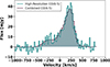 |
Fig. A.1. Comparison of the high-resolution CO(6−5) spectrum versus the spectrum from the combined dataset. Note: the spectral resolution between the two datasets was not the same. No significant difference is seen in the flux, suggesting that no emission has been filtered out in the high-resolution image. |
Appendix B: Lens modeling
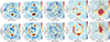 |
Fig. B.1. Nonparametric source modeling results for the blue and red bins of the CO(6−5) emission. First row: Blue peak in the CO(6−5) spectrum. Second row: Red peak in the CO(6−5) spectrum. The first column shows the dirty image as produced by PYAUTOLENS with contours shown at 3, 4, 5, 6, 7, 8, 9, 10σ levels. Note: this is not a cleaned image and structures may look slightly different than those shown in cleaned images. The second column shows the dirty model image as produced by PYAUTOLENS with contours shown at 3, 4, 5, 6, 7, 8, 9, 10σ levels. The third column shows the dirty residual image produced by PYAUTOLENS with contours shown at −3, −2, 2, 3, 4, 5σ levels. The fourth column shows the image plane emission nonparametric model of the data produced by PYAUTOLENS. The black line represents the critical line. The fifth column shows the source plane emission nonparametric model of the data produced by PYAUTOLENS. The black line represents the caustic line. All images are centered around the ALMA phase center for each image. Note: the H2O+ emission is of significantly lower angular resolution as the lensing model was created using the combined data, as described in Sect. 2. |
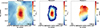 |
Fig. B.2. Source plane CO(6−5) masked and unmasked moment-0 and moment-1 maps created from the source plane emission cube described in Sect. 3.3.3. The first panel shows the full moment-0 map with contours shown at −3, −2, 3, 4, 5, 6, 7, 8, 9, 10σ levels. The middle panel shows the moment-0 map masked to show only values above 4σ levels where the contours are shown at 5, 6, 7, 8, 9, 10σ levels. The right panel shows the moment-1 map masked to show only values above 4σ levels. The intensity values are in arbitrary units for both the unmasked and masked moment-0 maps as output from PYAUTOLENS. The approximate beam, assuming a static magnification factor across the image, is shown in the bottom-left of each image. A clear velocity gradient is seen in the moment-1 emission map. |
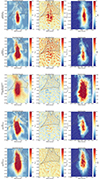 |
Fig. B.3. Source plane intensity (left panels), error map (middle panels), and S/N map (right panels) for the continuum (top), CO(6−5) (second row), CO(6−5) source plane emission cube (third row), H2O (fourth row), and H2O+ (bottom row) emission. The grey grid shows the Voronoi pixels prior to interpolation to the square pixel grid, as described in Sect. 3.3.3. The black line shows the caustic line. Note: the error maps have been normalized by the maximum value in the respective intensity map and, therefore, the error maps can be seen as a percentage error for each pixel. For the CO(6−5) source plane cube the intensity map is the source plane moment-0 map and the intensity map is a moment-0 map of the error cube as described in Sect. 3.3.3. Note: the S/N map is zoomed-in compared to the other two panels. |
Appendix C: Kinematic modeling
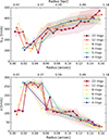 |
Fig. C.1. Rotational velocity and dispersion as a function of radius when varying the number of rings used in the 3DBAROLO kinematic modeling. The errors are represented by the shaded regions for both. |
All Tables
Best-fit lens parameters, optimized from parametric models of the dust continuum emission.
Best-fit parametric source modeling results for continuum and detected molecular line species.
All Figures
|
Fig. 1. Continuum image of G09v1.97, imaged using a natural weighting scheme. The contours are shown at −3, −2, 3, 4, 5, 6, 7, 8, 9, 10σ levels (σ = 0.02 mJy/beam). The black region shows the region from which the continuum emission was extracted. The synthesized beam is shown in the bottom- left of the image and corresponds to 0.11″ × 0.084″. |
| In the text | |
|
Fig. 2. Spectra of the detected molecular line species in G09v1.97. Top-left: CO(6−5) spectrum. Top-right: H2O spectrum. Bottom: H2O+ spectrum. Note: the H2O+ emission was not detected in the high-resolution data and, thus, the spectrum was taken from the combined data (as described in Sects. 2 and 3.2), resulting in a different spectral resolution than for the CO(6−5) and H2O emission. The spectrum for each molecule was extracted from a region corresponding to the region shown in Fig. 1. For each molecule, the spectrum is shown in the top panel, and the residuals from the Gaussian fits are shown in the lower panel. Single Gaussian profiles are shown in red, while double Gaussian profiles are shown in blue; similarly, in the lower panel, the residuals from fitting using a single Gaussian profile are shown in red and in blue for fits using two Gaussian profiles. It is clear that double Gaussian profiles offer a better fit of the spectra for all detected molecular line species. The dashed gray line in the top panel and the gray region in the lower panel represent the per-channel RMS. The top axis in the top panel for each spectrum shows the corresponding redshift. Note: the red residuals in the bottom panel are shown as slightly narrower (i.e., appearing to have a smaller channel width) than the blue, which is purely for clarity purposes. |
| In the text | |
|
Fig. 3. Moment-0 and moment-1 maps of the molecular line emission detected towards G09v1.97. Top: CO(6−5). Middle: H2O. Bottom: H2O+. The contours are shown at −3, −2, 3, 4, 5, 6, 7, 8, 9, 10σ levels for the CO(6−5) and H2O emission and at −3, −2, 3, 4, 5σ levels for the H2O+ emission. The synthesized beam is shown in the bottom- left of every image, beam sizes can be found in Table 1 for each line. Note: the angular resolution is significantly lower for the H2O+ emission as it was imaged from the combined dataset as described in Sect. 2. A clear velocity gradient is visible in the moment-1 map of the CO(6−5) emission. |
| In the text | |
|
Fig. 4. Comparison of the normalized CO(6−5), H2O, and H2O+ emission. Note: the noise appears significantly higher in the H2O+ emission due to the line’s lower S/N value. The line profiles of all three emission lines are very similar. |
| In the text | |
|
Fig. 5. Parametric lens and source modeling results for the detected emission towards G09v1.97. First row: Dust continuum. Second row: CO(6−5). Third row: H2O. Fourth row: H2O+ emission. The first column shows the dirty image as produced by PYAUTOLENS with contours shown at 3, 4, 5, 6, 7, 8, 9, 10σ levels, where 1σ is the rms of a blank region of the image. Note: this is not a cleaned image and structures may look slightly different than those shown in cleaned images. The second column shows the dirty model image as produced by PYAUTOLENS with contours shown at 3, 4, 5, 6, 7, 8, 9, 10σ levels. The third column shows the dirty residual image produced by PYAUTOLENS with contours shown at the −3, −2, 2, 3, 4, 5σ levels. The fourth column shows the image plane emission parametric model of the data produced by PYAUTOLENS. The white line represents the critical line. The fifth column shows the source plane emission parametric model of the data produced by PYAUTOLENS. The white line shows the caustic line. All images are centered around the ALMA phase center for each image. Note: the H2O+ emission is of significantly lower angular resolution as the lensing model was created using the combined data, as described in Sect. 2. |
| In the text | |
|
Fig. 6. Nonparametric source modeling results for the detected emission towards G09v1.97. First row: Dust continuum. Second row: CO(6−5). Third row: H2O. Fourth row: H2O+ emission. The first column shows the dirty image as produced by PYAUTOLENS with contours shown at 3, 4, 5, 6, 7, 8, 9, 10σ levels where 1σ is the rms of a blank region of the image. Note: this is not a cleaned image, and structures may look slightly different than those shown in cleaned images. The second column shows the dirty model image as produced by PYAUTOLENS with contours shown at 3, 4, 5, 6, 7, 8, 9, 10σ levels. The third column shows the dirty residual image produced by PYAUTOLENS with contours shown at −3, −2, 2, 3, 4, 5σ levels. The fourth column shows the image plane emission nonparametric model of the data produced by PYAUTOLENS. The black line shows the critical line. The fifth column shows the source plane emission nonparametric model of the data produced by PYAUTOLENS. The black lines show the caustic line. All images are centered around the ALMA phase center for each image. Note: the H2O+ emission is of significantly lower angular resolution as the lensing model was created using the combined data, as described in Sect. 2. |
| In the text | |
|
Fig. 7. Fitting results from 3DBAROLO with parameters set as described in Sect. 3.4. For all rows, the first column shows the data, the second the model, and the third the residual (data minus model). The first row shows the moment-0 emission (intensity), the second the velocity field (rotational velocity, Vrot), and the third the velocity dispersion (σ). The final 3DBAROLO ring is shown as the black ellipse and regions outside this ellipse are made semi-transparent to emphasize the region used for fitting. The major axis is shown in the first two rows by the dashed grey line. The kinematic center is shown by the green line in the first two columns of the second row. The approximate beam, assuming a static magnification factor across the image, is shown in the bottom-left of each image. |
| In the text | |
|
Fig. 8. PV diagrams from 3DBAROLO, upper: major axis, lower: minor axis. The blue contours show the contours of the data at 2, 3, 4, 5σ levels, and the red contours show the best-fit model to the data. In the major axis pv diagram, the yellow dots show the best fit rotational velocity in each of the rings. The right axis (VLOS) shows the velocities centered around the systemic velocity of the galaxy at the redshift of G09v1.97 (z = 3.63). The left axis (ΔVLOS) shows the velocities centered around the user-set systemic velocity, here 120 km/s (Table 5). |
| In the text | |
|
Fig. 9. Rotational velocity and dispersion as a function of radius for G09v1.97 for each ring in our 3DBAROLO fit. Red shows the rotational velocity and gray shows the dispersion. The errors are represented by the shaded regions for both. |
| In the text | |
|
Fig. 10. Source plane channel maps for the CO(6−5) emission from the demagnified source plane emission cube described in Sect. 3.3.3. The velocities covered by each bin are shown at the top of the image. The background mesh shows the Voronoi mesh pixels prior to interpolation to a square grid. Black line shows the caustic line. A clear velocity gradient is evident across the emission line. |
| In the text | |
|
Fig. 11. Comparison between the approximate image plane spectrum and source plane spectrum of the CO(6−5) emission in G09v1.97. Left: Source plane moment-0 map of the CO(6−5) emission with the different regions used for the source plane spectral extraction. Right: Normalized source plane spectrum (in yellow) compared to the normalized image plane spectrum (in grey) extracted from the region used in 3DBAROLO modeling (top), a northern region of the source located inside the caustic line (middle), and a southern region of the source located outside the caustic line (bottom). Note: the per-channel values are the normalized sum in a specific region as described in Sect. 4.1.1 and not a standard flux. The error bars are shown for each channel. Single Gaussian profiles are shown in red, while double Gaussian profiles are shown in blue. |
| In the text | |
|
Fig. 12. Top: Source plane contour plots of the dust continuum, CO(6−5), and H2O emission in G09v1.97. The contours are at 30, 40, 60, 80, 100% levels of the maximum value of the individual tracer. The approximate beam, assuming a static magnification factor across the image, is shown in the bottom- left of the image. Bottom: Normalized enclosed flux in circular apertures increasing from the center of the CO(6−5), dust continuum, and H2O emission out to 80% of the total flux of the image. It is clear that the dust continuum emission is the most compact of the emission types, whereas the CO(6−5) and H2O emission closely match in emission extent. |
| In the text | |
|
Fig. 13. Residual moment-0 and moment-1 maps from 3DBAROLO fitting and the S/N map of the emission using the source plane error map (i.e., source plane intensity/moment-0 divided by the source plane intensity error map) as described in Sect. 3.3.3. Note: the first two panels are a zoomed-in version of the same images shown as in Fig. 7 (rows 1 and 2, column 3), but with a different color scale. The grey grid shows the Voronoi pixels prior to interpolation to the square pixel grid, as described in Sect. 3.3.3. The black line shows the caustic line and the white ellipse shows the region used for 3DBAROLO fitting (i.e., the final ring). As in Fig. 7, any emission outside the fitting region is semi-transparent. The approximate beam, assuming a static magnification factor across the image, is shown in the bottom- left of the image. |
| In the text | |
|
Fig. 14. Evolution of V/σ with redshift for G09v1.97 (shown by the pink star) and literature sources. The literature sample is taken from Amvrosiadis et al. (2025), Roman-Oliveira et al. (2023), Hodge et al. (2012), Fraternali et al. (2021), Lelli et al. (2023), Liu et al. (2023), Neeleman et al. (2023), Parlanti et al. (2023), Posses et al. (2023), Rizzo et al. (2020, 2021, 2023), Rowland et al. (2024), Turner et al. (2017). For the literature sample, we show atomic tracers (in this case [C II], [O III], Hα emission) in yellow and molecular gas tracers (in this case, different CO transitions) in blue. We show the semi-analytic model from Wisnioski et al. (2015) in gray with Q values ranging between 0.67 to 2 and the fiducial model of Q = 1 in the dashed gray line. |
| In the text | |
|
Fig. A.1. Comparison of the high-resolution CO(6−5) spectrum versus the spectrum from the combined dataset. Note: the spectral resolution between the two datasets was not the same. No significant difference is seen in the flux, suggesting that no emission has been filtered out in the high-resolution image. |
| In the text | |
|
Fig. B.1. Nonparametric source modeling results for the blue and red bins of the CO(6−5) emission. First row: Blue peak in the CO(6−5) spectrum. Second row: Red peak in the CO(6−5) spectrum. The first column shows the dirty image as produced by PYAUTOLENS with contours shown at 3, 4, 5, 6, 7, 8, 9, 10σ levels. Note: this is not a cleaned image and structures may look slightly different than those shown in cleaned images. The second column shows the dirty model image as produced by PYAUTOLENS with contours shown at 3, 4, 5, 6, 7, 8, 9, 10σ levels. The third column shows the dirty residual image produced by PYAUTOLENS with contours shown at −3, −2, 2, 3, 4, 5σ levels. The fourth column shows the image plane emission nonparametric model of the data produced by PYAUTOLENS. The black line represents the critical line. The fifth column shows the source plane emission nonparametric model of the data produced by PYAUTOLENS. The black line represents the caustic line. All images are centered around the ALMA phase center for each image. Note: the H2O+ emission is of significantly lower angular resolution as the lensing model was created using the combined data, as described in Sect. 2. |
| In the text | |
|
Fig. B.2. Source plane CO(6−5) masked and unmasked moment-0 and moment-1 maps created from the source plane emission cube described in Sect. 3.3.3. The first panel shows the full moment-0 map with contours shown at −3, −2, 3, 4, 5, 6, 7, 8, 9, 10σ levels. The middle panel shows the moment-0 map masked to show only values above 4σ levels where the contours are shown at 5, 6, 7, 8, 9, 10σ levels. The right panel shows the moment-1 map masked to show only values above 4σ levels. The intensity values are in arbitrary units for both the unmasked and masked moment-0 maps as output from PYAUTOLENS. The approximate beam, assuming a static magnification factor across the image, is shown in the bottom-left of each image. A clear velocity gradient is seen in the moment-1 emission map. |
| In the text | |
|
Fig. B.3. Source plane intensity (left panels), error map (middle panels), and S/N map (right panels) for the continuum (top), CO(6−5) (second row), CO(6−5) source plane emission cube (third row), H2O (fourth row), and H2O+ (bottom row) emission. The grey grid shows the Voronoi pixels prior to interpolation to the square pixel grid, as described in Sect. 3.3.3. The black line shows the caustic line. Note: the error maps have been normalized by the maximum value in the respective intensity map and, therefore, the error maps can be seen as a percentage error for each pixel. For the CO(6−5) source plane cube the intensity map is the source plane moment-0 map and the intensity map is a moment-0 map of the error cube as described in Sect. 3.3.3. Note: the S/N map is zoomed-in compared to the other two panels. |
| In the text | |
|
Fig. C.1. Rotational velocity and dispersion as a function of radius when varying the number of rings used in the 3DBAROLO kinematic modeling. The errors are represented by the shaded regions for both. |
| In the text | |
Current usage metrics show cumulative count of Article Views (full-text article views including HTML views, PDF and ePub downloads, according to the available data) and Abstracts Views on Vision4Press platform.
Data correspond to usage on the plateform after 2015. The current usage metrics is available 48-96 hours after online publication and is updated daily on week days.
Initial download of the metrics may take a while.