| Issue |
A&A
Volume 708, April 2026
|
|
|---|---|---|
| Article Number | A194 | |
| Number of page(s) | 23 | |
| Section | Interstellar and circumstellar matter | |
| DOI | https://doi.org/10.1051/0004-6361/202557365 | |
| Published online | 08 April 2026 | |
Warps survive beyond fly-by encounters in protoplanetary disks
RW Aur A as a case study
1
Dipartimento di Fisica, Università degli Studi di Milano,
via Celoria 16,
20133
Milano,
Italy
2
Zentrum für Astronomie, Heidelberg University,
Albert-Ueberle-Str. 2,
69120
Heidelberg,
Germany
3
Departamento de Física, Universidad de Santiago de Chile,
Av. Víctor Jara 3493,
Santiago,
Chile
4
Millennium Nucleus on Young Exoplanets and their Moons (YEMS),
Chile
5
Center for Interdisciplinary Research in Astrophysics Space Exploration (CIRAS), Universidad de Santiago,
Chile
★ Corresponding author: This email address is being protected from spambots. You need JavaScript enabled to view it.
Received:
22
September
2025
Accepted:
29
January
2026
Abstract
Aims. Stellar fly-bys can have multiple dynamical effects on protoplanetary disks, including warping and the excitation of spiral arms. Since observations indicate that warps are common, we aim to investigate these effects for different fly-by trajectories. We further link our models to observations by applying them to the RW Aur system, which is a fly-by candidate with a well-constrained trajectory.
Methods. We investigated the disk dynamics in grid-based hydrodynamical simulations, which allow for a lower disk viscosity than in commonly used smoothed particle hydrodynamics models. We post-processed our simulations of the RW Aur system with radiative transfer models to create synthetic images of the dust continuum and gas kinematics.
Results. Fly-bys inclined with respect to the original disk plane can excite warps of a few degrees, but the exact outcome depends on the specific geometry of the encounter. Specifically, we find that the position of the periastron with respect to the initial disk plane plays a role in the resulting warp strength. Within our parameter set, the strongest warp is excited for a retrograde fly-by with a periastron that is not in the same plane as the disk. Our models show that the warp can persist even after the perturber can no longer be clearly linked to the system, implying that past fly-bys are a possible origin of observed warps. Excited spirals arms, on the other hand, are much more short-lived than a warp. We performed a simulation of the recent close encounter in the observed disk around RW Aur A, one of the few systems with a well-constrained trajectory. We find that a warp of about 5° can be excited and that the strong spiral arms have already disappeared at the current time of observation (300 yr after periastron). This compares well with existing continuum observations, and our synthetic kinematic evaluations hint at remnant structures in the gas density that may be detectable.
Key words: hydrodynamics / radiative transfer / methods: numerical / protoplanetary disks
© The Authors 2026
 Open Access article, published by EDP Sciences, under the terms of the Creative Commons Attribution License (https://creativecommons.org/licenses/by/4.0), which permits unrestricted use, distribution, and reproduction in any medium, provided the original work is properly cited.
This article is published in open access under the Subscribe to Open model. This email address is being protected from spambots. You need JavaScript enabled to view it. to support open access publication.
1 Introduction
Most stars are not born in isolated environments. Usually, they form in large star-forming regions, often in clusters of many thousand stars (Draine 2011; Krause et al. 2020). Observations have shown that these star-forming regions are highly dynamic, with significant relative velocities between stars (Karnath et al. 2019; Kuhn et al. 2019; Yang et al. 2025). Thus, young stars are likely to encounter other young stars (see, e.g., Pfalzner 2013; Bate 2018; Lebreuilly et al. 2021; Rawiraswattana & Goodwin 2023; Lebreuilly et al. 2024). These stars commonly host planet-forming disks, and therefore the interactions in a stellar cluster can affect the disk shape and morphology and in turn influence the process of planet formation (Kobayashi & Ida 2001; Fragner & Nelson 2009; Thies et al. 2010; Breslau & Pfalzner 2019; Cuello et al. 2019; Aly & Lodato 2020; Aly et al. 2021; Longarini et al. 2021).
Close encounters of stars on unbound orbits are commonly referred to as stellar fly-bys. Often, a fly-by is defined as having a separation between the two stars of less than 1000 au (Cuello et al. 2023). As the occurrence rate of fly-bys is highest when the objects are still spatially confined to their star-forming region, the probability at which disk-hosting stars experience close gravitational interactions with other stars in their lifetime can be as high as 70%, depending on the stellar density (Winter et al. 2018, see their Fig. 7). Cuello et al. (2023) conclude in their review, that more than half of young stars hosting a disk experience a fly-by with a separation of less than 1000 au.
Stellar fly-bys have a significant impact on the dynamics and morphology of the disks around either one or both of the fly-by components. One of the first numerical studies of the effect of fly-bys on circumstellar disks was performed by Clarke & Pringle (1993), and the topic has been extensively investigated since. These effects include spiral arms due to tidal perturbations (Ostriker 1994; Pfalzner 2003; Cuello et al. 2019; Smallwood et al. 2023); truncation of disk sizes (Breslau et al. 2014; Rosotti et al. 2014; Muñoz et al. 2015; Vincke et al. 2015; Bhandare et al. 2016); ejection and capture of disk material by the fly-by object (Heller 1995; Jílková et al. 2016; Cuello et al. 2019, 2020; Smallwood et al. 2024); and misalignment and warping of disks (Terquem & Bertout 1993; Picogna & Marzari 2014; Xiang-Gruess 2016; Nealon et al. 2020).
The resulting shape of the disk depends on the geometry of the fly-by orbit with respect to the disk. Fly-by trajectories are typically classified as prograde, retrograde, or polar, depending on the direction of the angular momentum vectors of the orbit and the disk. For prograde fly-bys, both vectors are in the same hemisphere, and in retrograde fly-bys, they are in opposite hemispheres. Mutual orientations of these vectors close to 90° are referred to as polar. Prograde orbits have been found to be the most disruptive (Clarke & Pringle 1993; Xiang-Gruess 2016; Winter et al. 2018). In prograde cases, the spirals caused by the tidal torques are the strongest, and the truncation of the disks is the most effective. For example, Bhandare et al. (2016) find for retrograde orientations that disk sizes after truncation can be twice as large as for prograde fly-bys. A characteristic signature of retrograde non-coplanar fly-bys is a warp due to the misaligned gravitational torque (Terquem & Bertout 1993; Xiang-Gruess 2016; Nealon et al. 2020; Cuello et al. 2023), although disks can also become warped in inclined prograde fly-bys (see, e.g., Larwood 1997).
Warps in protoplanetary disks have gained importance throughout recent years, as an ever-increasing amount of observations have revealed indications that a significant fraction of disks are warped (Ansdell et al. 2020; Kluska et al. 2020; Bohn et al. 2022; Garufi et al. 2022; Benisty et al. 2023; Winter et al. 2025). For example, non-axisymmetric shadows can hint at a misaligned inner region of the disk that blocks the light from the star (Marino et al. 2015; Benisty et al. 2017; Debes et al. 2017; Stolker et al. 2017; Muro-Arena et al. 2020; Villenave et al. 2024; Zurlo et al. 2024, and many more). Indications for warps can also be found in kinematic observations (Walsh et al. 2017; Mayama et al. 2018; Phuong et al. 2020; Garg et al. 2021; see also Pinte et al. 2023 for a review). After initial excitation, the evolution of the warp shape is controlled by internal torques. These torques arise from pressure gradients and resonant motions that form due to the mutual misalignment of radially adjacent orbits (Ogilvie & Latter 2013a,b; Dullemond et al. 2022). The evolution of the warp depends on the viscosity and the disk thickness, characterized by the Shakura-Sunyaev parameter α (Shakura & Sunyaev 1973) and the aspect ratio h, respectively. In thick disks with low viscosity (α < h), the warp travels in a wave through the disk (Papaloizou & Lin 1995; Lubow & Ogilvie 2000; Nixon & King 2016; Martin et al. 2019; Kimmig & Dullemond 2024). In more viscous disks, where α > h, the warp evolves diffusively (Papaloizou & Pringle 1983; Pringle 1992; Ogilvie 1999). In typical protoplanetary disks, the viscosity is low relative to the aspect ratio, placing them in the wave-like regime.
Most numerical studies investigate the effects of fly-bys utilizing smoothed particle hydrodynamics (SPH) simulations (see Picogna & Marzari 2014; Xiang-Gruess 2016; Cuello et al. 2019; Ménard et al. 2020; Nealon et al. 2020, etc.) because these simulations do not rely on a specific geometry for the discretization. However, SPH methods usually need to include an artificial viscosity that is often higher than the physical viscosities found in protoplanetary disks (for example by Villenave et al. 2024). In light of the recent development (Rabago et al. 2023, 2024; Kimmig & Dullemond 2024), we take the opportunity to focus on grid-based hydrodynamic models of low-viscosity disks subjected to a stellar fly-by. Stellar fly-bys provide an ideal laboratory for investigating the evolution of warps, as they create a physically motivated warp shape instead of a parameterized assumption and only distort the disk once, without further influence of external torques.
As an additional motivation for our work, we aim to explore different orientations of trajectories with respect to the disk plane. Recent studies have mainly investigated orientations where the trajectory is inclined in such a way that the periastron remains in the same plane as the disk (Cuello et al. 2019; Nealon et al. 2020; Cuello et al. 2023). This is likely motivated by the fact that Xiang-Gruess (2016) found that for the final mean tilt of the disk, the inclination of the trajectory with respect to the disk is more relevant than the relative position of the periastron. However, the radial inclination profile could be strongly affected by the position of the periastron. In young stellar clusters, there is no physical constraint that the periastron should be in the same plane as the disk. In fact, a scenario with the periastron outside the disk plane should be statistically more likely.
In the first part of this work, we therefore revisit a limited set of disk-orbit orientations to compare the effects on the warping of the disk. We describe our numerical setup in Section 2 and present the results of the hydrodynamical investigations in Section 3. In the second part, we apply the models to the observed RW Aur system and present synthetic observations in Section 4. We discuss our work in Section 5 and conclude in Section 6.
2 Numerical method
2.1 Hydrodynamic simulations
If a nearby star approaches a disk close enough, its gravitational pull begins to notably impact the dynamics of the disk. In cases where the fly-by trajectory is inclined relative to the disk plane, this interaction can generate a warp. To investigate the dynamical effect of fly-bys on low-viscosity disks, we performed 3D hydrodynamic simulations using the grid-based code FARGO3D (Benítez-Llambay & Masset 2016; Masset 2000), where we include a gravitational perturber on a parabolic orbit modeled with the built-in orbit solver.
We ran gas-only simulations and did not make use of the multi-fluid or magnetohydrodynamic features of the code. For the viscosity, we used an α-viscosity model (Shakura & Sunyaev 1973) with the dimensionless parameter α = 10−3. The capability of the code to model warps and disk planes inclined with respect to the grid geometry was extensively tested in Kimmig & Dullemond (2024).
We modeled the hydrodynamics on a spherical grid (r, θ, ϕ). Radially, the grid extends from 2.6 au to 41.6 au with 120 logarithmically spaced grid cells. In the azimuthal direction, we use 100 cells. Vertically, we capped off the poles in order to save computation time and include a range of θmin = 44.2° to θmax = 135.8° (where θ = 90° corresponds to the initial disk midplane) with 256 vertical grid cells.
We set up an initially planar (unwarped) disk, which is aligned with the grid midplane. To ensure the disk remains unaffected by the outer radial boundary, we taper its density profile so that it lies well within the computational domain. We therefore adopted for the initial surface density Σ profile
![Mathematical equation: $\[\Sigma(r)=\Sigma_0\left(\frac{r}{r_0}\right)^{-p}\left[1+\exp \left(\frac{r-r_{\text {out }}}{0.05 r_{\text {out }}}\right)\right]^{-1}\left[1+\exp \left(\frac{r_{\text {in }}-r}{0.05 r_{\text {in }}}\right)\right]^{-1},\]$](/articles/aa/full_html/2026/04/aa57365-25/aa57365-25-eq1.png) (1)
(1)
where Σ0 is the surface density at the reference radius r0, for which we used r0 = 5.2 au. The equation includes exponential cut-offs at both disk edges, where rin and rout are the inner and outer edge of the disk, respectively. Unless specified otherwise, we use rin = 3.12 au to rout = 26 au, a slope of p = 1, and a total disk mass of Mdisk = 0.02 M⊙, which leads to a surface density Σ0 = 209 g/cm2 at r0. Since the disk-to-star mass ratio lies below 0.5, gravitational instability is not expected to be relevant. Earlier work demonstrates that self-gravity can modify the warp evolution and damping in low-viscosity disks (Papaloizou & Lin 1995). Yet, wave-like warp propagation is also expected when self-gravity is negligible (Papaloizou & Terquem 1995). To avoid additional complexity, we neglect self-gravity in our models. To vertically expand the surface density, we use the default setup of the example p3disof from FARGO3D.
We assumed a locally isothermal model, where we set the temperature structure so that the aspect ratio h takes the form
![Mathematical equation: $\[h(r)=h_0\left(\frac{r}{r_0}\right)^f,\]$](/articles/aa/full_html/2026/04/aa57365-25/aa57365-25-eq2.png) (2)
(2)
with h0 being the aspect ratio at r0 and the flaring index f. For all our models, we use the values h0 = 0.05 and f = 0.25. The initial azimuthal velocity is set to the Keplerian velocity with a correction for pressure gradients, as described in Appendix A.
In all simulations, we adopted outflow boundaries for the radial direction, where we allowed mass to leave the grid domain but not to enter. This means that the radial velocity is copied from the active domain edge to the ghost cells if positive, but forced to zero if negative. This helps to avoid unphysical influx of gas, which has sometimes been found to occur in fly-by scenarios especially at the inner boundary. Vertically, we set reflective boundaries and azimuthally periodic conditions.
We set the grid origin to the central star hosting the disk. Therefore, we needed to account for non-inertial motion of the reference frame due to the fly-by. This is taken care of with the build-in indirect term in FARGO3D. However, we did not treat any non-inertial effects imposed by a possible acceleration from the disk onto the star, for example due to asymmetries in the disk. As disks in fly-bys can become very asymmetric due to the spirals and the warping, this could potentially have an effect on the dynamics. However, the detailed physics and the correct implementation of this indirect term are still under investigation (Crida et al. 2025; Jordan & Rometsch 2025), and we decided to neglect this effect for now.
2.2 Fly-by geometry
The trajectory of the fly-by is described in Cartesian coordinates. We define the x-y-plane to coincide with the initial disk midplane. A convenient way to describe the trajectory orientation are the orbital elements, which are the three angles indicated in Figure 1. We call the inclination between trajectory and disk plane θ. The longitude of ascending node Ω is the angle between the x-axis and the intersection line between the plane of the trajectory within the x-y-plane, and the argument of periapsis ω is the angle between the intersection line and the connecting line of origin to periapsis. We note that physically, the longitude of ascending node Ω does not make a difference in our simulations, as the disk is initially axisymmetric, which means that the setup would lead to the same result for different Ω, only rotated.
The trajectory of the fly-by is calculated by FARGO3D with a fifth-order Runge-Kutta N-body solver and we only set the initial position and velocity of the star on the fly-by trajectory, called perturber from here on. In addition to the orbital elements, the trajectory is characterized by the distance of periapsis (or closest approach) rp and the orbit eccentricity e. For the simulations, we choose the initial distance dini between the two stars and then calculate the initial position and velocity of the perturber using the hyperbolic equation. More details are given in Appendix B.
3 Parameter exploration
In this section, we explore a limited set of fly-by configurations. We aim to investigate the dynamical effects of a fly-by on the disk, where we focus on disk warping. We do not intend to cover the full parameter space, nor do we intend to maximize the warp strength of the disk, but instead choose a set of representative test cases.
Specifically, we decided on two different geometric configurations, depicted in Figure 2. For simplicity, we define the trajectories in both configurations such that the perturber comes from the positive x-direction, leading to a periapsis in the negative x-regime. For the first configuration, the periapsis lies in the same plane as the disk and the trajectory is rotated about the x-axis, corresponding to a longitude of ascending node of Ω1 = 0° and an argument of periapsis ω1 = 180° (see Figure 1 for the definition of these angles). The second configuration is rotated about the y-axis, and therefore Ω2 = 90° and ω2 = 90°. We set the inclination of the trajectories in both cases to θ1,2 = 30°.
For both configurations, we perform both a prograde and a retrograde fly-by. Here we note that technically, the definition of the longitude of ascending node Ω would change for the retrograde orbit, as the ascending node flips by 180°. However, for simplicity, we use the same angles to describe both prograde and retrograde orbits and simply flip the starting point of the perturber. For comparison, we additionally perform a coplanar orbit (with Ω = 90°, ω = 90°, and θ = 0°), also both prograde and retrograde.
Throughout this work, we define t = 0 to be the moment of the closest approach between the two stars. We initialized our simulations at t = −2012 yr, which allows for about 15 orbits at the outer disk edge (r = 26 au) before the closest approach. Most simulations end at t = 1995 yr, when the perturber has roughly reached the same distance as in the beginning.
In all six simulations, we set the distance of the closest approach at the periapsis to rp = 104 au. We model parabolic fly-bys with an eccentricity of e = 1, and set the initial distance of the perturber from the disk-hosing star to dini = 1040 au, so that the disk has enough time to relax from the initial conditions. All six simulations model an equal mass fly-by, where q = Mfl/M* = 1. Here, M* corresponds to the disk-hosting star and Mfl to the mass of the perturber. We set M* = Mfl = 1 M⊙ for both stars.
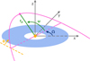 |
Fig. 1 Schematics of the definition for the geometry of the fly-by trajectory with respect to the disk plane. Indicated are the inclination of the trajectory, θ; the longitude of the ascending node, Ω; and the argument of periapsis, ω. The distance of the closest approach (i.e., the periapsis) is rp. |
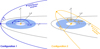 |
Fig. 2 Trajectory configurations for our fly-by simulations. The disk lies in the x-y-plane at the origin of the coordinate system with a counter-clockwise rotation. Configuration 1 is shown in blue on the left, where the trajectory is rotated about the x-axis with a periapsis in the same plane as the disk. Configuration 2 (orange, right) is rotated about the y-axis with a periapsis out of the disk plane. |
3.1 Disk warping
We can characterize the warping of the disk by studying the evolution of the inclination profile. Analogously to Kimmig & Dullemond (2024), we computed the angular momentum vector of each radial shell of the grid and computed the inclination at each radius as the angle between the local angular momentum vector and the z-axis.
Figure 3 shows the inclination evolution for both configurations for pro- and retrograde orbits. We checked that the inclination of the disk for a coplanar fly-by does not change, which means that the disk does not warp in these cases, as expected.
Fly-bys on an inclined trajectory, however, all induce a change of the disk inclination with a small warp in most cases. Only the retrograde case for Configuration 1, where the trajectory is tilted about the x-axis (but the periastron is in the disk’s midplane), inhibits almost no warp. Here, the disk tilts rigidly by about 2°. In the other three simulations, the disk becomes warped, and the warp travels in a wave through the disk. This wave shows the typical standing wave behavior of the global bending modes with a wavelength of 2 rout. In addition to the warp, we find a twist, or in other words, a differential precession of the disk. Details are given in Appendix C.1.
Both prograde simulations show features in addition to the warp wave that are excited around the time of the closest approach. These features move outward and dissipate quickly and are likely linked to the spiral arms that are excited more strongly in prograde fly-bys. We take a closer look at the spiral arms in Section 3.2.
To investigate the mean tilt of the disk due to the fly-by, we evaluated the mean inclination in each simulation by computing the angle of the total angular momentum vector with respect to the z-axis. Figure 4 shows the evolution of the mean tilt for all simulations. All inclined fly-bys induce a mean tilt of close to 2°, irrespective of the exact geometry of the trajectory. This is consistent with the results by Xiang-Gruess (2016), who find that the absolute value of the inclination, θ, of the orbit with respect to the disk is the decisive quantity determining the final mean tilt of the disk. From looking at the inclination profiles, however, we find that the warping of the disk very much depends on the exact orientation of the trajectory. In particular, the warp is stronger for the retrograde case in Configuration 2, where the periapsis does not lie in the same plane as the disk. Because the warp is strongest in this simulation (a maximum misalignment of about 4°), we decided to investigate this simulation on longer timescales. In this way, we can study the decay of the warp after the perturber has left the system. Figure 5 shows the evolution of the orbital plane inclination at r = 23.9 au, which is close to the outer edge of the disk.
The decay of the warp can be estimated by fitting
![Mathematical equation: $\[f(t)=A ~\cos (\omega t-b) \times \exp \left(-\lambda_{\mathrm{d}} t\right)+c+d ~t,\]$](/articles/aa/full_html/2026/04/aa57365-25/aa57365-25-eq3.png) (3)
(3)
where A is the amplitude parameter, ω is the frequency, λd is the decay rate, b is a possible phase shift, c is an offset that corresponds to the mean tilt, and d is a linear damping in overall inclination. The last parameter is included for possible inclination damping due to the grid, as found in Kimmig & Dullemond (2024). However, in our simulations with such a low warp amplitude, we find almost no damping, that is, d = 10−5 deg yr−1. For the fit, we used the scipy-function curve_fit (Virtanen et al. 2020).
We find that some level of warping is still present after the perturber is already long gone. The mean lifetime of the warp is around τ = 1/λd ≈ 1.4 × 10⁴ yr and the period of the warp wave about T = 103 yr. This aligns with theoretical estimates, as the damping of the warp can be approximated with linear theory τliner theory = 1/(αΩout) ≈ 2 × 10⁴ yr, where Ωout is the Keplerian frequency evaluated at the outer edge of the disk (Lubow & Ogilvie 2000). In addition to viscosity, a hydrodynamic instability called “parametric instability” (Gammie et al. 2000) is known to enhance the dissipation of the warp amplitude (Deng et al. 2021; Fairbairn & Ogilvie 2023; Held & Ogilvie 2026). Our analysis of the vertical velocity in our simulations suggests that the parametric instability may be present at early times before the close encounter (see Appendix D). At later times, however, the perturbation in the vertical velocity induced by the fly-by becomes so strong that it would mask any such instability, even if it were present. Additionally, the resolution in our simulation is too low to resolve the parametric instability in detail. Thus, we are unable to conclusively determine whether the instability is present.
The period of the warp can be estimated with the wave speed of the warp τwarp wave = Δr/vwarp ≈ 700 yr, where Δr = rout − rin and vwarp = cs/2 (e.g., Nixon & King 2016). Specifically, the fact that the warp period found in our simulation is longer means that the warp wave is propagating slower than the propagation speed predicted by analytical theory. This difference partly arises as the analytic prediction was derived under the assumption of a completely inviscid disk (Papaloizou & Terquem 1995; Ogilvie 2006). Further nonlinear effects might contribute to the difference.
We noticed a period change after about 1.6 × 10⁴ yr and stopped the fit of the warp decay at that time. A period change is not physically expected in the evolution of an undriven warp (see, e.g., Kimmig & Dullemond 2024). In this case of a fly-by event, the change could be caused by a change in disk structure. However, it could also be a numerical effect.
In summary, inclined fly-bys can excite warps and twists that remain even after the perturber has reached a distance greater than 1000 au. This can mean for observations that for warps triggered by a fly-by, the fly-by object is not necessarily associated with the perturbed system. We find moderate warp strengths of ≤ 4°. However, the warp can be stronger for different fly-by parameters, i.e., a shorter distance of closest approach, a more massive fly-by object, or more inclined trajectories. Although it would be interesting to find parameters to maximize the excited warp, it is not the focus of this study.
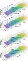 |
Fig. 3 Inclination evolution of the fly-by simulations with the prograde and retrograde fly-by of Configuration 1 (periastron in the same plane as the disk) in the top two panels and Configuration 2 (periastron out of disk plane) in the bottom two panels. Time t = 0 indicates the moment of closest approach. The color corresponds to time, and the blue and orange vertical dashed lines indicate the times when the perturber crosses the (initial) disk midplane. We note that we plot the inclination profile only up to the outer radius of the disk rout = 26 au, but the computational domain extends further out. |
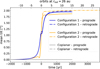 |
Fig. 4 Mean tilt defined as the angle between the total angular momentum vector of the disk and the z-axis for all six trajectory configurations. |
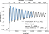 |
Fig. 5 Evolution of the orbital plane at r = 23.9 au in the retrograde simulation in Configuration 2 (see Figure 2, right). We started the fit according to Equation (3) (blue dashed line) at the first maximum of the curve (dashed gray line) and stopped the fit at t = 1.58 × 10⁴ yr, where the period seems to change. We note that this figure shows the evolution over a longer time period than Figure 3. |
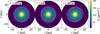 |
Fig. 6 Surface density snapshots of the prograde fly-by in Configuration 2. Time t = 0 yr is the point of the closest approach. The gray dashed circle indicates a radius of 15 au, where we performed further analysis of the spirals. Further snapshots are shown in Appendix C.3. |
3.2 Spirals
Fly-bys are known to create spirals due to tidal effects (Clarke & Pringle 1993; Ostriker 1994). Figure 6 shows snapshots of the vertically integrated density (per radial shell) before, during, and after the close encounter of the prograde simulation in Configuration 2. In addition to spirals, fly-bys are also known to truncate the disk. However, the disk in our simulation is already compact in the beginning, which is why we do not find truncation (see Appendix C.2).
We investigated the spirals in more detail by measuring the strength of the spirals in all six different setups. For that, we extracted the maximum value of the surface density Σpeak at a single radial location over time, analogous to Smallwood et al. (2023), and scaled it with the mean surface density Σmean at that radius. Figure 7 shows the evolution of this peak surface density, which indicates the strength of the spirals, in all of our simulations at r = 15 au.
We find that strong spirals occur for all three prograde setups. The retrograde simulations, on the other hand, show little or no spirals, consistent with previous findings (e.g., Clarke & Pringle 1993; Cuello et al. 2019, 2023). We thus focus on the prograde simulations for the further evaluation in this section.
The strongest spirals occur for the coplanar prograde orbit. The simulation with the orbit tilted with respect to the x-axis (Configuration 1), where the periastron is in-plane, follows with the second strongest spirals. Configuration 2, with a periastron outside of the disk plane, shows the weakest of the three prograde fly-bys. This is consistent with the findings of Smallwood et al. (2023), see their Figure 14 (but we note that their setup is defined rotated by 90°, so that their rotation about the x-axis corresponds to the case with the periastron out-of plane).
We then investigated the azimuthal evolution of the spirals in Figure 8, where we plot an azimuthal cut at the same radius, r = 15 au, over time. In all simulations, the spirals are extremely short-lived and only last about 500 yr. At the time where the spirals dissolve, the perturber is located at a distance of about 370 au from the disk-hosting star, which are roughly 3.6 rp.
In comparison to Smallwood et al. (2023), the spirals in our simulations dissolve faster on physical timescales. As the disk in their simulations has properties different from our setup, we perform a quick analysis of timescale estimations here. Smallwood et al. (2023) find a lifetime of about 5000 yr for a disk ranging from 10–100 au. The outer disk has an orbital time scale of about 1000 yr, which means that the outer disk performs about five orbits during the lifetime of the spirals. In our simulations, the spirals live roughly 500 yr in a disk ranging from 2–26 au, leading to an orbital period of 130 yr at the outer disk edge, which is slightly fewer than four orbits during the spiral lifetime. This compares well with the five orbits found by Smallwood et al. (2023). In this context, we want to point out that the fact that the spirals live longer than the longest orbital timescale in the disk indicates that the spiral shape is not purely caused by the Keplerian shear of a density wave.
Additional differences between our simulations and Smallwood et al. (2023) are the disk viscosity, which is smaller by at least a factor of two in our simulations and the flaring of the disk. Smallwood et al. (2023) set up an unflared (often called flat) disk with a constant aspect ratio of Hp/r = 0.05, whereas we set our temperature structure such that the disk is flared with an index of 0.25. These factors could also have an impact on the lifetime of the spirals. Furthermore, Smallwood et al. (2023) focus on less massive perturbers than we do, but for the lifetime of the spirals they do not find any strong dependency on the perturber mass.
The lifetime of the spirals in our simulations coincides with the lifetime of the additional features in the inclination profile for the prograde simulations (as seen in Figure 3). If the spirals are warped, they could cast shadows. As the spirals significantly change on observable timescales, this could possibly lead to an evolution of shadow features on short timescales, as observed in a few disks, for example in TW Hya (Debes et al. 2017), HD 135344B (Stolker et al. 2017), or MWC 758 (Ren et al. 2020).
All in all, we find that the spirals are much more short-lived than the warp. For observations this means that the fly-by scenario cannot be ruled out as the origin for observed warps, even in the absence of a nearby companion or an accompanying spiral pattern.
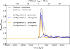 |
Fig. 7 Time evolution of the peak surface density at r = 15 au in all six simulations. Prograde simulations are shown with solid lines, while retrograde simulations are indicated with dash-dotted lines. |
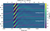 |
Fig. 8 Azimuthal cut of the vertically integrated surface density at r = 15 au for all three prograde simulations. The pink line indicates the angle to the perturber projected to the x–y-plane. The time axis is scaled such that t = 0 yr indicates the point of the closest approach. |
4 Observational signatures: Models of RW Aur
In this part of this work, we aspire to create links between our numerical models and observations. Observationally, ongoing stellar fly-bys are proposed for quite a few systems, for example in SR 24 (Weber et al. 2023; Mayama et al. 2010, 2020; Fernández-López et al. 2017), FU Ori (Takami et al. 2018; Pérez et al. 2020; Borchert et al. 2022), Z CMa (Dong et al. 2022), UX Tau (Ménard et al. 2020; Zapata et al. 2020), AS 205 (Kurtovic et al. 2018), and more (see Tab. 1 and Fig. 6 in Cuello et al. 2023). Because a general investigation of observational signatures of fly-bys requires a large parameter space of disk orientations with respect to the observer (which would go beyond the scope of this work), we decided to apply our models to a specific observed system: RW Aur (Ghez et al. 1993).
The RW Aur system is a two-star system where both stars host a disk (Cabrit et al. 2006; Rodriguez et al. 2018; Long et al. 2019), and the projected separation between the stars is about 233 au. A recent study by Kurtovic et al. (2024, hereafter Kur24) performed a detailed orbital fitting using astrometric data from different epochs, which offers good constraints for our models. Kur24 find an eccentricity close to e ≈ 1, which could either be a highly eccentric bound orbit or a close-to-parabolic unbound orbit. For the sake of this work, we assumed an unbound trajectory, even though Kur24 find that bound orbits are slightly favored.
The work by Kur24 presented ALMA dust continuum observations with high angular resolution of the two disks around A and B. For the geometry of the disks, they performed Markov chain Monte Carlo fitting and found disk inclinations of iA = 55° and iB = 64°. Both disks have a position angle of about PAB = 39.5°, and under the assumption that the near side is the same for both disks, the mutual inclination can be determined from the difference of inclinations to be about 9°.
In their analysis of the observations, Kur24 find indications of a warp in the disk around RW Aur A, as they find a peculiar pattern in the residuals between the observations and a planar (unwarped) parametric model. Kur24 are able to minimize the residuals with a model including a misaligned inner disk1 of 3 au with an inclination of iA,inn = 60.8° and a position angle of PAA,inn = 35.5°. This results in a misalignment between inner and outer disk of roughly 6°. A warp in RW Aur A was even suspected prior to this study (Bozhinova et al. 2016; Facchini et al. 2016b), as observations suggested a mismatch between the inclination of the inner and outer disks (inner disk2: 77° by Eisner et al. 2007, >60° by McJunkin et al. 2013; outer disk: 45° − 60° by Woitas et al. 2001 and Rodriguez et al. 2013).
Millimeter observations of CO gas in the system additionally reveal a large-scale structure connecting the two stars (Cabrit et al. 2006) and a chaotic environment (Rodriguez et al. 2018, Kur24). Cabrit et al. (2006) proposed this large-scale structure to be a tidal arm caused by a recent close encounter of star B with the disk around star A, which has later been supported by hydrodynamical simulations (Dai et al. 2015).
4.1 Hydrodynamic models
In this section, we present hydrodynamic models as described in Section 2. For the disk around RW Aur A, we set up an initially planar disk with a range from 1.2–20 au and an inner grid domain extended to 1 au. In order to keep the resolution consistent with the simulations in Section 3, we increased the number of radial cells to 160. The orbital period at the outer edge of the disk is 80 yr. The chosen disk size corresponds to the size of the observed dust disk at λ = 1.3 mm in the system (Kur24), as we aim for radiative transfer models in the millimeter wavelength range tracing the dust continuum. We note, however, that the size of the observed gas disk is larger by a factor of about two. Additionally, observations suggest that the disk extends to an inner edge at 0.1 au, while our inner radius is set to 1.2 au. However, smaller cavities become computationally costly in grid-based simulations, which is why we settled for a larger inner radius.
For the masses of the stars, we used MA = 1.238 M⊙ and MB = 0.995 M⊙ of star A and B, respectively, leading to a mass ratio of q = MB/MA = 0.8037. For the gas disk mass, we assumed Mgas = 0.01 MA. We kept the slope of the surface density and the temperature structure (and hence the vertical shape of the disk) the same as in our previous models. This gave a surface density of Σ0 = 179 g/cm2 at the reference radius of r0 = 5.2 au. As in the previous models, we set the disk viscosity to α = 10−3.
For the geometric setup of the fly-by, we use the parameters for disk and orbit reported by Kur24 with inclination id, out = 54.8 deg and position angle of PAd, out = 39.4° for the outer edge of the disk and an orbit inclination io = 129.8°, a position angle Ωo = 73.8°, and an argument of periapsis ωo = 42.3°. The distance of closest approach is rp = 55 au. We note that these orbital parameters are given in the reference frame of the sky. For the grid-based hydrodynamical simulations, however, it is best for the disk to initially lie in the x-y-plane. We therefore needed to compute the respective geometry of the orbital parameters with respect to the disk plane3. The detailed steps for the calculation of the angles can be found in Appendix E. For the eccentricity, Kur24 report e= 0.787 for their best fit. In our models, we set e = 1 for an unbound orbit.
We find a mutual inclination between the orbit and the outer disk plane to be θmut = −27.5°, where the minus sign indicates that the periastron is below the disk plane in our simulations. This value for the mutual inclination is also reported by Kur24. For the argument of periastron with respect to the disk plane, we find ωmut = 86.3°. At this point, we can set the longitude of ascending node arbitrarily, as the disk is initially axisymmetric. However, this angle will become important for the radiative transfer simulations, where we need to project the model to the sky plane in order to calculate synthetic observations. Because we do not expect a mean disk tilt of more than a few degrees, we set up the models such that the disk initially lies in the plane of the observed outer disk.
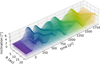 |
Fig. 9 Evolution of the inclination profile for the simulation of the disk around RW Aur A. The color indicates the time; time t = 0 indicates the point of the closest approach. |
4.1.1 Warping of the disk
Figure 9 shows the evolution of the inclination profile for the simulation adapted to RW Aur. The disk develops a warp with a maximum misalignment of about 5°, which aligns nicely with the observed indications of a 6° misalignment between inner and outer disk found by Kur24. As expected, the warp travels as a wave through the disk in our simulations. We find a final mean inclination (defined as the angle between the total angular momentum vector and the z-axis) of 2.6°. The evolution of the inclination profile shows a pattern that suggests that multiple superimposed bending waves are present.
Compared to Figure 3, the warp is slightly stronger and the wave evolves on shorter timescales. Although the geometry of the fly-by trajectory is similar to Configuration 2 in the previous part of this work, there are some important differences. First, the disk is smaller in size, with an outer radius of rout = 20 au instead of 26 au. This for example influences the warp timescale, which is sensitive to the disk size because of the reflection of the warp wave at the disk edges. Further, the host star has a larger mass, whereas the perturber has a lower mass than in the previous simulations. The distance of closest approach is shorter with rp = 55 au instead of 104 au. Figure 10 shows a cross-section through the disk at the current point of time, where the warped structure is visible.
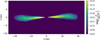 |
Fig. 10 Cross-section of the gas density in the model of RW Aur A at the current time (295 yr after periastron). |
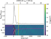 |
Fig. 11 Peak surface density (top panel) and azimuthal profile evolution (bottom panel) of the RW Aur simulation at r = 15 au. As in Figure 8, the pink line indicates the angle to the perturber. The dashed yellow line highlights the current point of time at t = 295 yr after periastron. |
4.1.2 Spirals
As the fly-by in the RW Aur system is prograde, we expect the excitation of spiral arms. Figure 11 shows the peak surface density (top), as well as the azimuthal density evolution (bottom) in the disk at a radius of r = 15 au.
We find that strong spirals are excited roughly at the point of the closest approach. As before, the spirals are short-lived. They disappear after roughly 200 yr, which corresponds to 2.5 orbits at the outer disk edge. At this time, the perturber is about 200 au away from the disk-hosting star. This is slightly shorter than the four orbits of the outer disk edge we found in Figure 8. The likely reason for this is the aforementioned differences in the model setup of disk size, disk and stellar masses, and trajectory parameters. We emphasize that the absolute strength of the spirals in the top panel is not trivially comparable to the previous simulations, as we chose the same plotting radius of r = 15 au for both parts, but the disk size differs.
4.1.3 Comparison to other work
Hydrodynamic models of a fly-by in the RW Aur system were performed a decade ago by Dai et al. (2015) using SPH. Their focus was the observed large-scale tidal arm that seems to link star A and B. One of their main results was that a prograde encounter was necessary in order to produce such a tidal arm, which aligns very well with the findings of the astrometric orbit fitting by Kur24. In order to produce the tidal arm, they set up an initially larger disk of 60 au, which is then truncated by the fly-by. When comparing the orbital parameters, their best model is similar to the result of the astrometric fit, and therefore to the setup in our work, as shown in Table 1. The good match of the orbital parameters is not a given, as Dai et al. (2015) fitted the orbital parameters so that their model matched the observed large-scale tidal arm.
Comparing the hydrodynamic results of the disk in detail is difficult, as the disk properties differ strongly, also shown in Table 1. A similarity we find are the excited spirals, which is not surprising given the prograde nature of both fly-by setups. Looking at their Figure 4, the spirals also seem to be short-lived and seem to dissolve within 200 yr after periastron passage. A direct comparison of the warping is not possible, as they did not explicitly analyze the warp. However, we expect the warp evolution to differ for models of different viscosity (Kimmig & Dullemond 2024). In the simulations by Dai et al. (2015), the viscosity is larger by at least a factor of two. However, the fact that the trajectory parameters are similar might indicate that if our initial disk size (and the computational domain) were larger, we would reproduce a similar large-scale tidal structure in our simulations.
Comparison of simulation setups.
4.2 Radiative transfer models of the dust continuum
In this section, we aim to compare our models to the observations. For this, we run Monte Carlo simulations using the radiative transfer code RADMC-3D (Dullemond et al. 2012). The dust temperature is calculated consistently with the radiative transfer model using the Monte Carlo Bjorkman & Wood (2001) method implemented in RADMC-3D, where we use the modified random walk option (Fleck & Canfield 1984), that accelerates the computation of photon packages in optically very thick regions by applying the analytical solution of the diffusion equation. We use 108 photon packages to compute the temperature. We then compute the sky model of the system with ray-tracing (also 108 photon packages) and produce synthetic images by convolving the fluxes with a two-dimensional Gaussian imitating the corresponding telescope’s finite resolution. We use a beam size of 18 × 30 mas and a position angle of 8.186°, as reported for the observational data. We note that to remain consistent with the observations by Kur24, we use a value of 154 pc for the distance to RW Aur A (Gaia Collaboration 2016, 2021), instead of the 156.1 pc found in the Gaia Data Release 3 (Gaia Collaboration 2023).
We compared the simulation with the ALMA dust continuum observations. For the composition of the dust, we assumed the DIANA standard composition of 87% carbon and 13% pyroxene, where the pyroxene is composed of molecule bonds with 70% magnesium and 30% iron. The porosity was set to 25% (Woitke et al. 2016). We computed the dust opacity and scattering matrices with optool (Dominik et al. 2021).
Since the hydrodynamic simulation only models gas, we needed to assume a spatial dust distribution in the disk. Because the behavior of larger dust particles in warping disks is not well known yet, we assumed small dust grains of a singular size a = 1 μm that are perfectly coupled to the gas. The choice of a singular dust size in contrast to a dust size distribution was motivated by the lack of good observational constraints on the actual size distribution. Additionally, it allowed us to ensure that the dust follows the dynamics of the gas.
For the dust-to-gas ratio, we aimed to match the total flux of the observation, which Kur24 reported to be 34.5 ± 0.01 mJy. With a dust-to-gas ratio of 10−2 (and a distance of 154 pc to the source), our radiative transfer model results in a total flux of 31.5 mJy, and we therefore adopted this dust-to-gas ratio. However, we note that our choice of a single grain size of small dust could underestimate the flux. We also note that the dust-to-gas ratio is somewhat flexible, as the total gas disk mass in our hydrodynamic simulations is scalable, as we do not treat self-gravity nor the indirect term from the disk onto the star. This means that the same total flux can also be reached when the gas disk mass and dust-to-gas ratio are scaled differently.
According to the fit by Kur24, the time of observation was t = 295 yr after the periastron. We confirmed in our simulation that the position of the perturber matches the observed position of RW Aur B. Figure 12 shows a comparison of the model next to the observation by Kur24. Both images are observed at a wavelength of λ = 1.3 mm. Overall, the images compare well. In the observations, the emission in the central beam is stronger roughly by a factor of 1.5, which could be because of our choice of a larger cavity in the simulation for reasons of computation time. We present the comparison between the convolved and unconvolved model in Appendix F.2, which shows that a few spiral features close to the inner edge are visible, which are then hidden by the beam resolution. A fine-tuned quantitative match is out of the scope of this work, as many parameters, such as disk characteristics, fly-by trajectory and dust models, have an impact on the result of the model.
In Figure 13, we present radiative transfer simulations at different times of the hydrodynamic simulation. During the point of closest approach (t = 0 yr), the spiral structure excited by the fly-by is indeed visible, but quickly disappears. The system is (synthetically) observed from the same location at each time, which corresponds to inclination and position angle of the initial setup of the simulation. The warp only changes the disk plane by a few degrees throughout the simulation, and therefore the observed inclination of the disk does not vary strongly. However, a slight variation of the inclination and position angle on a time scale of a few tens of years could be observable.
One of the objectives of the comparison between the simulations and the real observation is whether the spiral structures produced by the fly-by should be observable with state-of-the-art instruments. At t = 295 yr in our simulations, the strongest spirals have already dissolved, as we show in Figure 11. In the simulations by Dai et al. (2015), the spirals seem to be weak as well at the time of comparison. However, some weak spiral structures are still residue in our simulations, also seen in the unconvolved image in Figure F.3. After the convolution (Figure 12), however, we find that these structures are not discernible, leading to the good match between model and observation.
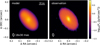 |
Fig. 12 Synthetic observation of our hydrodynamic simulation at t = 295 yr after periastron at a wavelength of λ = 1.3 mm (left panel) next to the ALMA Band 6 observation of RW Aur (right panel, Kurtovic et al. 2024), which is also at λ = 1.3 mm. The ellipse in the bottom-left corner indicates the beam and is the same for both images. |
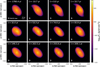 |
Fig. 13 Synthetic observations at λ = 1.3 mm of the RW Aur A simulation at different times. The first panel shows the initial setup of the simulation, time t = 0 yr is the time of the closest approach, and the current time step lies between the second last and last panels. The images were convolved with the same beam as Figure 12. |
4.3 Synthetic gas kinematics
Observations of molecular lines can give insight into the gas dynamics of protoplanetary disks (see, e.g., Pinte et al. 2023). The kinematic structure can be highly complex (Teague et al. 2025). We investigate the kinematic structures in the RW Aur system due to the recent close encounter in line radiative transfer models using RADMC-3D.
We chose the J=2–1 rotational transition of 12CO at λ = 1.3 mm and computed 200 channels in a window of ±20 km/s around the molecular line. For the molecular abundance, we assumed a number density fraction 12CO/H2 = 10−4. We took into account the CO-depletion via freeze-out for temperatures lower than 20 K (Williams & Best 2014). For that, we assumed the gas to be thermally coupled with the dust and computed the dust temperature using the Bjorkmann & Wood method. We further included the photodissociation effect for column number densities lower than a threshold value (Visser et al. 2009). We chose a threshold of Ndissoc = 5 × 10¹⁹ H2/cm2, which is in alignment with the range found by Trapman et al. (2023) and Rosotti et al. (2025). To compute the vertical column density, we used an interpolation from our spherical grid. Then, we set the abundance to zero wherever the column density drops below the threshold. To save computation time, we neglect scattering effects for the line radiative transfer.
Unfortunately, a detailed comparison to actual observations of the RW Aur system is not useful at this point, as the currently available kinematic observations do not possess sufficient spectral resolution to show details in the kinematics (see, e.g., Kur24). We keep the kinematic images unconvolved for now, and all moment maps were created with the unclipped data. In this section, we focus on the current time at 295 yr after periastron passage.
Figure 14 shows some of the resulting velocity channels from the line radiative transfer model. Recall that the upper right side (north-west) is the near side of the disk. Many channels show interesting “wiggly” features that clearly deviate from a usual model of a smooth disk. We investigate these features further by computing moment maps.
The left panel of Figure 15 shows the Moment 0 map. In contrast to the dust continuum images presented in Section 4.2, it clearly shows a disturbed structure. The emission of the observed 12CO-line originates in the upper layers of the disk, as opposed to the dust continuum, which typically traces the disk midplane. This indicates that the disk surfaces are more disturbed than the disk midplane. In the map of the velocity of the peak intensity (also called Moment 9 map, Figure 15, right), the v = 0 km/s-line (white) also appears to be wiggly. To investigate this in more detail, we subtracted a Keplerian disk model to reveal the residuals, shown in Figure 16. For the Keplerian disk model, we used the initial setup of our hydrodynamic simulation, for which we computed a kinematic data cube in the same way using RADMC-3D. The velocity of the peak intensity of this is shown in Appendix F.2, Figure F.4.
The deviation from a Keplerian model is significant and we find complex dynamical features in the residuals. Some of these features might originate from remnants of the spirals that were excited during the fly-by event. The warped morphology of the disk may also affect the kinematic structure. While a further detailed analysis to disentangle these effects is highly relevant in the current development of the field (e.g., Pinte et al. 2023; Teague et al. 2025), it would go beyond the scope of this work, and we thus have to leave it for future work. At this point, we also want to note that the observed gas disk of RW Aur A is larger than in our hydrodynamic model. We chose the more compact size in order to match the dust continuum observations when assuming that the dust is evenly distributed. For a better analysis of the kinematics in the RW Aur system with predictions for observations, considering a larger gas disk could be helpful. However, the results of this section show that better kinematic observations of the RW Aur system could very well reveal remnant features of the recent close encounter and provide further insight into the dynamics of the system.
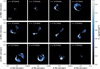 |
Fig. 14 Intensity of different velocity channels of the RW Aur A model at the current time of 295 yr after periastron passage. |
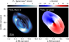 |
Fig. 15 Moment 0 map (left) and velocity of the peak intensity (Moment 9, right) of the gas in the hydrodynamic model of the disk around RW Aur A at 295 yr after periastron. The line is centered at v = 0 km/s, which corresponds to proper motion corrected observations. |
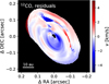 |
Fig. 16 Deviation from a Keplerian profile of the Moment 9 map shown in the right panel of Figure 15. |
5 Discussion
5.1 Fly-bys as potential origin of moderate warps
Our hydrodynamical models show that warps of a few degrees are a natural consequence of fly-bys with an inclined trajectory with respect to the disk plane. The persistence of the warp beyond the actual fly-by encounter raises the fly-by scenario as possibility for the origin of observed moderate warps, even if no perturber can be dynamically associated with the system. In fact, moderate warps might be the rule rather than the exception in protoplanetary disks. For example, Winter et al. (2025) found indications of warps in the kinematics of almost all disks of the exoALMA sample (Teague et al. 2025). In alignment with that, Villenave et al. (2024) observed asymmetries in near IR observations in 15/20 disks observed edge-on. These asymmetries are likely created by moderate warps of a few degrees (Kimmig & Villenave 2025).
That said, the damping of the warp highly depends on the disk viscosity (Nixon & King 2016; Kimmig & Dullemond 2024, see also Appendix F.1). This means that the warp persists longer than the fly-by event only in low-viscosity disks (α ≤ 10−3 as rough reference). Therefore, it is crucial to account for low-viscosity scenarios in models, which highlights the need for grid-based simulations to complement SPH models, that usually cannot represent physical viscosities of α below a few times 10−3 (see Lodato & Price 2010; Meru & Bate 2012).
However, an inclined stellar fly-by is not the only possible cause for a warped disk and the origin of moderate warps remains unknown. Alternative formation scenarios include misaligned infall of material onto the disk (Thies et al. 2011; Dullemond et al. 2019; Kuffmeier et al. 2024), misaligned magnetic fields with respect to the disk plane (Foucart & Lai 2011; Romanova et al. 2021), radiation-induced warping (for stars with L ≳ 10 L⊙) (Pringle 1996; Armitage & Pringle 1997), misaligned binaries (Facchini et al. 2013; Lodato & Facchini 2013; Deng & Ogilvie 2022; Rabago et al. 2024), or outer bound companions such as stars or planets (Papaloizou & Lin 1995; Nealon et al. 2018; Zanazzi & Lai 2018; Zhu 2019).
5.2 Implications and caveats in the RW Aur case
For the application to RW Aur, we assumed an unbound fly-by trajectory, even though Kurtovic et al. (2024) find that bound orbits are more likely by a factor of 0.28. In general, the effect of highly eccentric orbits is expected to be similar to that of unbound orbits (Cuello et al. 2023). We performed a quick timescale estimation. The best fit of Kurtovic et al. (2024) includes an eccentricity of e = 0.78 and leads to an orbital period of approximately 2800 yr. In our simulations, the excited warp is expected to still be present after this time, which means that a repeated encounter due to the bound nature of the orbit could create a different warp structure than a single fly-by. However, since the maximum amplitude of the warp is only of a few degrees and strongly dampened during one orbital period, our results might still be viable even for the bound case.
In the event of a close encounter, strong UV radiation from the fly-by perturber can influence the dynamics of the disk (Guarcello et al. 2023). This UV radiation radiation can cause photoevaporation (Winter & Haworth 2022), which plays a decisive role in disk evolution (e.g., Clarke 2007; Facchini et al. 2016a; Winter et al. 2018; Keyte & Haworth 2025). However, in the case of RW Aur A, we do not expect strong radiation onto the disk, as the perturber is of relatively low mass. Nevertheless, shadows in the disk due to the warp could influence the dynamics by changing the temperature structure of the disk (Su & Bai 2024; Zhang & Zhu 2024; Ziampras et al. 2025).
Interestingly, a jet is observed in the RW Aur system (Hirth et al. 1994; Alencar et al. 2005; Melnikov et al. 2009). Jets are thought to be linked to magnetic fields and could indicate magnetohydrodynamic winds launched from the disk. Magnetic fields likely influence the dynamics of warped disks. So far, warping of protoplanetary disks under the influence of magnetic fields has not been well studied. Jets can also replenish the interstellar material in these environments, which can affect nearby disks that accrete this material for example through streamers (Pineda et al. 2020; Ginski et al. 2021; Codella et al. 2024; Cacciapuoti et al. 2024).
An interesting fact worth mentioning is that RW Aur A is found to have an unusually high accretion rate of about 10−7 M⊙/yr (Hartigan et al. 1995). Cabrit et al. (2006) suggested the recent fly-by as possible explanation, as fly-bys could be able to trigger episodes of increased accretion (so-called FU Orionis events Bonnell & Bastien 1992; Pfalzner 2008; Forgan & Rice 2010). Even though strictly speaking RW Aur A is not an FU Orionis object, according to the formal definition (see, e.g., Connelley & Reipurth 2018), accretion episodes could still play a role for the star and disk. Additionally, several dimming events have been observed for RW Aur A (Rodriguez et al. 2013, 2016; Antipin et al. 2015; Petrov et al. 2015) which have been suggested to be caused by surrounding disrupted material (Rodriguez et al. 2013; Dodin et al. 2019) or a warp in the disk (Bozhinova et al. 2016; Facchini et al. 2016b).
6 Conclusion
In this work, we have performed simulations of inclined fly-bys passing a protoplanetary disk, and our focus was placed on the warping of the disk. In our simulations, we chose to model parabolic orbits (e = 1) where the velocity at the periastron is lowest in comparison to other unbound orbits. This means that parabolic fly-bys are expected to have the largest influence on the disk. Our main findings are outlined as follows:
we find that inclined fly-bys can trigger a warp of a few degrees, which evolves in a wave-like manner through the disk and lasts much longer than the fly-by itself. The warping is the most prominent in fly-bys where the periastron is not in the same plane as the disk, especially in a retrograde fly-by. This is particularly interesting since the warping in such fly-by configurations is not well studied yet;
the lifetime of spirals, which are excited especially in prograde configurations, is much shorter than that of the warp, with the spirals lasting only about four orbits of the outer disk. Observationally, this means that a warp triggered by a fly-by could still be observed when the fly-by object is long out of sight and no obvious spiral structures are observed in the disk. In other words, fly-bys may provide an explanation for some of the observed moderate warps;
we applied the stellar fly-by scenario to the RW Aur system, where a recent (about 300 yr ago) close encounter between two stars hosting a disk is suspected to have occurred. Recent orbital fitting by Kurtovic et al. (2024) gives good constraints on the mutual geometry of the fly-by trajectory with respect to the disk, which we used to set up our simulations. We find that the trajectory of RW Aur B around the RW Aur A is likely to induce a warp of around 5° in the disk around star A, which is consistent with observational indications of a misalignment between inner and outer disk regions of 6°;
radiative transfer simulations of our hydrodynamic model enabled a comparison of the resulting dust continuum to the observations. We find that in the dust continuum wavelengths (λ = 1.3 mm), the disk in our model looks smooth and the spirals are not visible, which compares well to the observation of the dust continuum of RW Aur A. Further, we found interesting features in the synthetic CO-line images that hint toward valuable insights that can be gained from future kinematic observations of this system.
In summary, this work shows that fly-bys might be able to explain frequently observed warps and shadow features in protoplanetary disks. Depending on the disk properties, the warp can remain present for longer timescales so that the perturber might not always be observable.
Acknowledgements
We kindly thank N. Kurtovic, T. Rometsch, L.-A. Hühn, I. Rabago, M. Leemker, G. Lodato, H. Klahr, and R. Klessen for their support and helpful comments. We remember the legacy of Prof. Willy Kley, who passed away in 2021, and would have been a part of this work. We acknowledge funding from the DFG research group FOR 2634 “Planet Formation Witnesses and Probes: Transition Disks” under grant DU 414/23-2 and KL 650/29-1, 650/29-2, 650/30-1. GR and CK acknowledge support from the European Union (ERC Starting Grant DiscEvol, project number 101039651) and from Fondazione Cariplo, grant No. 2022-1217. SF acknowledges financial contribution from the European Union (ERC, UNVEIL, 101076613) and from PRIN-MUR 2022YP5ACE. Views and opinions expressed are, however, those of the author(s) only and do not necessarily reflect those of the European Union or the European Research Council. Neither the European Union nor the granting authority can be held responsible for them. PW acknowledges support from FONDECYT grant 3220399 and ANID – Millennium Science Initiative Program – Center Code NCN2024_001. Additionally, we acknowledge support by the High Performance and Cloud Computing Group at the Zentrum für Datenverarbeitung of the University of Tübingen, the state of Baden-Württemberg through bwHPC and the German Research Foundation (DFG) through grant INST 37/935-1 FUGG. This paper makes use of the following ALMA data: ADS/JAO.ALMA#2018.1.00973.S ALMA is a partnership of ESO (representing its member states), NSF (USA) and NINS (Japan), together with NRC (Canada), MOST and ASIAA (Taiwan), and KASI (Republic of Korea), in cooperation with the Republic of Chile. The Joint ALMA Observatory is operated by ESO, AUI/NRAO and NAOJ. Parts of this work were included in a PhD thesis. Plots in this paper were made with the Python (Van Rossum & Drake 2009) library matplotlib (Hunter 2007). We acknowledge also the usage of numpy (Harris et al. 2020), scipy (Virtanen et al. 2020) and astropy (Astropy Collaboration 2022). We acknowledge the use of CARTA (Comrie et al. 2018) for preliminary visualization and exploration of data.
References
- Alencar, S. H. P., Basri, G., Hartmann, L., & Calvet, N. 2005, A&A, 440, 595 [NASA ADS] [CrossRef] [EDP Sciences] [Google Scholar]
- Aly, H., & Lodato, G. 2020, MNRAS, 492, 3306 [Google Scholar]
- Aly, H., Gonzalez, J.-F., Nealon, R., et al. 2021, MNRAS, 508, 2743 [NASA ADS] [CrossRef] [Google Scholar]
- Ansdell, M., Gaidos, E., Hedges, C., et al. 2020, MNRAS, 492, 572 [Google Scholar]
- Antipin, S., Belinski, A., Cherepashchuk, A., et al. 2015, Inform. Bull. Variable Stars, 6126, 1 [Google Scholar]
- Armitage, P. J., & Pringle, J. E. 1997, ApJ, 488, L47 [Google Scholar]
- Astropy Collaboration (Price-Whelan, A. M., et al.) 2022, ApJ, 935, 167 [NASA ADS] [CrossRef] [Google Scholar]
- Bate, M. R. 2018, MNRAS, 475, 5618 [Google Scholar]
- Benisty, M., Stolker, T., Pohl, A., et al. 2017, A&A, 597, A42 [NASA ADS] [CrossRef] [EDP Sciences] [Google Scholar]
- Benisty, M., Dominik, C., Follette, K., et al. 2023, in Astronomical Society of the Pacific Conference Series, Vol. 534, Protostars and Planets VII, eds. S. Inutsuka, Y. Aikawa, T. Muto, K. Tomida, & M. Tamura, 605 [Google Scholar]
- Benítez-Llambay, P., & Masset, F. S. 2016, APJS, 223, 11 [CrossRef] [Google Scholar]
- Bhandare, A., Breslau, A., & Pfalzner, S. 2016, A&A, 594, A53 [NASA ADS] [CrossRef] [EDP Sciences] [Google Scholar]
- Bjorkman, J. E., & Wood, K. 2001, ApJ, 554, 615 [NASA ADS] [CrossRef] [Google Scholar]
- Bohn, A. J., Benisty, M., Perraut, K., et al. 2022, A&A, 658, A183 [NASA ADS] [CrossRef] [EDP Sciences] [Google Scholar]
- Bonnell, I., & Bastien, P. 1992, ApJ, 401, L31 [Google Scholar]
- Borchert, E. M. A., Price, D. J., Pinte, C., & Cuello, N. 2022, MNRAS, 510, L37 [Google Scholar]
- Bozhinova, I., Scholz, A., Costigan, G., et al. 2016, MNRAS, 463, 4459 [NASA ADS] [CrossRef] [Google Scholar]
- Breslau, A., & Pfalzner, S. 2019, A&A, 621, A101 [NASA ADS] [CrossRef] [EDP Sciences] [Google Scholar]
- Breslau, A., Steinhausen, M., Vincke, K., & Pfalzner, S. 2014, A&A, 565, A130 [NASA ADS] [CrossRef] [EDP Sciences] [Google Scholar]
- Cabrit, S., Pety, J., Pesenti, N., & Dougados, C. 2006, A&A, 452, 897 [CrossRef] [EDP Sciences] [Google Scholar]
- Cacciapuoti, L., Macias, E., Gupta, A., et al. 2024, A&A, 682, A61 [NASA ADS] [CrossRef] [EDP Sciences] [Google Scholar]
- Clarke, C. J. 2007, MNRAS, 376, 1350 [NASA ADS] [CrossRef] [Google Scholar]
- Clarke, C. J., & Pringle, J. E. 1993, MNRAS, 261, 190 [Google Scholar]
- Codella, C., Podio, L., De Simone, M., et al. 2024, MNRAS, 528, 7383 [NASA ADS] [CrossRef] [Google Scholar]
- Comrie, A., Wang, K.-S., Hwang, Y.-H., et al. 2018, https://doi.org/10.5281/zenodo.18477253 [Google Scholar]
- Connelley, M. S., & Reipurth, B. 2018, ApJ, 861, 145 [NASA ADS] [CrossRef] [Google Scholar]
- Crida, A., Baruteau, C., Griveaud, P., et al. 2025, Open J. Astrophys., 8, 84 [Google Scholar]
- Cuello, N., Dipierro, G., Mentiplay, D., et al. 2019, MNRAS, 483, 4114 [Google Scholar]
- Cuello, N., Louvet, F., Mentiplay, D., et al. 2020, MNRAS, 491, 504 [Google Scholar]
- Cuello, N., Ménard, F., & Price, D. J. 2023, Eur. Phys. J. Plus, 138, 11 [NASA ADS] [CrossRef] [Google Scholar]
- Dai, F., Facchini, S., Clarke, C. J., & Haworth, T. J. 2015, MNRAS, 449, 1996 [Google Scholar]
- Debes, J. H., Poteet, C. A., Jang-Condell, H., et al. 2017, ApJ, 835, 205 [NASA ADS] [CrossRef] [Google Scholar]
- Deng, H., & Ogilvie, G. I. 2022, MNRAS, 512, 6078 [NASA ADS] [CrossRef] [Google Scholar]
- Deng, H., Ogilvie, G. I., & Mayer, L. 2021, MNRAS, 500, 4248 [Google Scholar]
- Dewberry, J. W., Latter, H. N., Ogilvie, G. I., & Fromang, S. 2025, Open J. Astrophys., 8, 158 [Google Scholar]
- Dodin, A., Grankin, K., Lamzin, S., et al. 2019, MNRAS, 482, 5524 [NASA ADS] [CrossRef] [Google Scholar]
- Dominik, C., Min, M., & Tazaki, R. 2021, OpTool: Command-line driven tool for creating complex dust opacities, Astrophysics Source Code Library [record ascl:2104.010] [Google Scholar]
- Dong, R., Liu, H. B., Cuello, N., et al. 2022, Nat. Astron., 6, 331 [NASA ADS] [CrossRef] [Google Scholar]
- Draine, B. T. 2011, Physics of the Interstellar and Intergalactic Medium (Princeton University Press) [Google Scholar]
- Dullemond, C. P., Juhasz, A., Pohl, A., et al. 2012, RADMC-3D: A multi-purpose radiative transfer tool, Astrophysics Source Code Library [record ascl:1202.015] [Google Scholar]
- Dullemond, C. P., Küffmeier, M., Goicovic, F., et al. 2019, A&A, 628, A20 [NASA ADS] [CrossRef] [EDP Sciences] [Google Scholar]
- Dullemond, C. P., Isella, A., Andrews, S. M., Skobleva, I., & Dzyurkevich, N. 2020, A&A, 633, A137 [EDP Sciences] [Google Scholar]
- Dullemond, C. P., Kimmig, C. N., & Zanazzi, J. J. 2022, MNRAS, 511, 2925 [NASA ADS] [CrossRef] [Google Scholar]
- Eisner, J. A., Hillenbrand, L. A., White, R. J., et al. 2007, ApJ, 669, 1072 [NASA ADS] [CrossRef] [Google Scholar]
- Facchini, S., Lodato, G., & Price, D. J. 2013, MNRAS, 433, 2142 [Google Scholar]
- Facchini, S., Clarke, C. J., & Bisbas, T. G. 2016a, MNRAS, 457, 3593 [Google Scholar]
- Facchini, S., Manara, C. F., Schneider, P. C., et al. 2016b, A&A, 596, A38 [NASA ADS] [CrossRef] [EDP Sciences] [Google Scholar]
- Fairbairn, C. W., & Ogilvie, G. I. 2021a, MNRAS, 505, 4906 [Google Scholar]
- Fairbairn, C. W., & Ogilvie, G. I. 2021b, MNRAS, 508, 2426 [Google Scholar]
- Fairbairn, C. W., & Ogilvie, G. I. 2023, MNRAS, 520, 1022 [NASA ADS] [CrossRef] [Google Scholar]
- Fernández-López, M., Zapata, L. A., & Gabbasov, R. 2017, ApJ, 845, 10 [CrossRef] [Google Scholar]
- Fleck, Jr., J. A., & Canfield, E. H. 1984, J. Computat. Phys., 54, 508 [Google Scholar]
- Forgan, D., & Rice, K. 2010, MNRAS, 402, 1349 [CrossRef] [Google Scholar]
- Foucart, F., & Lai, D. 2011, MNRAS, 412, 2799 [NASA ADS] [CrossRef] [Google Scholar]
- Fragner, M. M., & Nelson, R. P. 2009, A&A, 505, 873 [NASA ADS] [CrossRef] [EDP Sciences] [Google Scholar]
- Gaia Collaboration (Brown, A. G. A., et al.) 2016, A&A, 595, A2 [NASA ADS] [CrossRef] [EDP Sciences] [Google Scholar]
- Gaia Collaboration (Brown, A. G. A., et al.) 2021, A&A, 649, A1 [NASA ADS] [CrossRef] [EDP Sciences] [Google Scholar]
- Gaia Collaboration (Vallenari, A., et al.) 2023, A&A, 674, A1 [NASA ADS] [CrossRef] [EDP Sciences] [Google Scholar]
- Gammie, C. F., Goodman, J., & Ogilvie, G. I. 2000, MNRAS, 318, 1005 [NASA ADS] [CrossRef] [Google Scholar]
- Garg, H., Pinte, C., Christiaens, V., et al. 2021, MNRAS, 504, 782 [Google Scholar]
- Garufi, A., Dominik, C., Ginski, C., et al. 2022, A&A, 658, A137 [NASA ADS] [CrossRef] [EDP Sciences] [Google Scholar]
- Ghez, A. M., Neugebauer, G., & Matthews, K. 1993, AJ, 106, 2005 [NASA ADS] [CrossRef] [Google Scholar]
- Ginski, C., Facchini, S., Huang, J., et al. 2021, ApJ, 908, L25 [NASA ADS] [CrossRef] [Google Scholar]
- Gonzalez, J.-F., van der Plas, G., Pinte, C., et al. 2020, MNRAS, 499, 3837 [Google Scholar]
- Guarcello, M. G., Drake, J. J., Wright, N. J., et al. 2023, ApJS, 269, 13 [NASA ADS] [CrossRef] [Google Scholar]
- Harris, C. R., Millman, K. J., van der Walt, S. J., et al. 2020, Nature, 585, 357 [NASA ADS] [CrossRef] [Google Scholar]
- Hartigan, P., Edwards, S., & Ghandour, L. 1995, in Revista Mexicana de Astronomia y Astrofisica Conference Series, 3, eds. M. Pena, & S. Kurtz, 93 [Google Scholar]
- Held, L. E., & Ogilvie, G. I. 2026, MNRAS, 546, stag245 [Google Scholar]
- Heller, C. H. 1995, ApJ, 455, 252 [NASA ADS] [CrossRef] [Google Scholar]
- Hirth, G. A., Mundt, R., Solf, J., & Ray, T. P. 1994, ApJ, 427, L99 [NASA ADS] [CrossRef] [Google Scholar]
- Hunter, J. D. 2007, Comput. Sci. Eng., 9, 90 [NASA ADS] [CrossRef] [Google Scholar]
- Jílková, L., Hamers, A. S., Hammer, M., & Portegies Zwart, S. 2016, MNRAS, 457, 4218 [Google Scholar]
- Jordan, L. M., & Rometsch, T. 2025, A&A, 693, A177 [NASA ADS] [CrossRef] [EDP Sciences] [Google Scholar]
- Karnath, N., Prchlik, J. J., Gutermuth, R. A., et al. 2019, ApJ, 871, 46 [NASA ADS] [CrossRef] [Google Scholar]
- Keyte, L., & Haworth, T. J. 2025, MNRAS, 537, 598 [Google Scholar]
- Kimmig, C. N., & Dullemond, C. P. 2024, A&A, 689, A45 [NASA ADS] [CrossRef] [EDP Sciences] [Google Scholar]
- Kimmig, C. N., & Villenave, M. 2025, A&A, 698, A146 [NASA ADS] [CrossRef] [EDP Sciences] [Google Scholar]
- Kluska, J., Berger, J. P., Malbet, F., et al. 2020, A&A, 636, A116 [NASA ADS] [CrossRef] [EDP Sciences] [Google Scholar]
- Kobayashi, H., & Ida, S. 2001, Icarus, 153, 416 [NASA ADS] [CrossRef] [Google Scholar]
- Krause, M. G. H., Offner, S. S. R., Charbonnel, C., et al. 2020, Space Sci. Rev., 216, 64 [CrossRef] [Google Scholar]
- Kuffmeier, M., Pineda, J. E., Segura-Cox, D., & Haugbølle, T. 2024, A&A, 690, A297 [NASA ADS] [CrossRef] [EDP Sciences] [Google Scholar]
- Kuhn, M. A., Hillenbrand, L. A., Sills, A., Feigelson, E. D., & Getman, K. V. 2019, ApJ, 870, 32 [CrossRef] [Google Scholar]
- Kurtovic, N. T., Pérez, L. M., Benisty, M., et al. 2018, ApJ, 869, L44 [Google Scholar]
- Kurtovic, N. T., Facchini, S., Benisty, M., et al. 2024, A&A, 692, A155 [NASA ADS] [CrossRef] [EDP Sciences] [Google Scholar]
- Larwood, J. D. 1997, MNRAS, 290, 490 [NASA ADS] [Google Scholar]
- Lebreuilly, U., Hennebelle, P., Colman, T., et al. 2021, ApJ, 917, L10 [NASA ADS] [CrossRef] [Google Scholar]
- Lebreuilly, U., Hennebelle, P., Colman, T., et al. 2024, A&A, 682, A30 [NASA ADS] [CrossRef] [EDP Sciences] [Google Scholar]
- Lodato, G., & Facchini, S. 2013, MNRAS, 433, 2157 [NASA ADS] [CrossRef] [Google Scholar]
- Lodato, G., & Price, D. J. 2010, MNRAS, 405, 1212 [NASA ADS] [Google Scholar]
- Long, F., Herczeg, G. J., Harsono, D., et al. 2019, ApJ, 882, 49 [Google Scholar]
- Longarini, C., Lodato, G., Toci, C., & Aly, H. 2021, MNRAS, 503, 4930 [Google Scholar]
- Lubow, S. H., & Ogilvie, G. I. 2000, ApJ, 538, 326 [CrossRef] [Google Scholar]
- Marino, S., Perez, S., & Casassus, S. 2015, ApJ, 798, L44 [Google Scholar]
- Martin, R. G., Lubow, S. H., Pringle, J. E., et al. 2019, ApJ, 875, 5 [NASA ADS] [CrossRef] [Google Scholar]
- Masset, F. 2000, A&ASS, 141, 165 [NASA ADS] [CrossRef] [EDP Sciences] [Google Scholar]
- Mayama, S., Tamura, M., Hanawa, T., et al. 2010, Science, 327, 306 [NASA ADS] [CrossRef] [Google Scholar]
- Mayama, S., Akiyama, E., Panić, O., et al. 2018, ApJ, 868, L3 [NASA ADS] [CrossRef] [Google Scholar]
- Mayama, S., Pérez, S., Kusakabe, N., et al. 2020, AJ, 159, 12 [NASA ADS] [CrossRef] [Google Scholar]
- McJunkin, M., France, K., Burgh, E. B., et al. 2013, ApJ, 766, 12 [Google Scholar]
- Melnikov, S. Y., Eislöffel, J., Bacciotti, F., Woitas, J., & Ray, T. P. 2009, A&A, 506, 763 [NASA ADS] [CrossRef] [EDP Sciences] [Google Scholar]
- Ménard, F., Cuello, N., Ginski, C., et al. 2020, A&A, 639, L1 [EDP Sciences] [Google Scholar]
- Meru, F., & Bate, M. R. 2012, MNRAS, 427, 2022 [NASA ADS] [CrossRef] [Google Scholar]
- Muñoz, D. J., Kratter, K., Vogelsberger, M., Hernquist, L., & Springel, V. 2015, MNRAS, 446, 2010 [CrossRef] [Google Scholar]
- Muro-Arena, G. A., Benisty, M., Ginski, C., et al. 2020, A&A, 635, A121 [NASA ADS] [CrossRef] [EDP Sciences] [Google Scholar]
- Nealon, R., Dipierro, G., Alexander, R., Martin, R. G., & Nixon, C. 2018, MNRAS, 481, 20 [Google Scholar]
- Nealon, R., Cuello, N., & Alexander, R. 2020, MNRAS, 491, 4108 [NASA ADS] [Google Scholar]
- Nixon, C., & King, A. 2016, in Lecture Notes in Physics, 905 (Berlin Springer Verlag), eds. F. Haardt, V. Gorini, U. Moschella, A. Treves, & M. Colpi, 45 [Google Scholar]
- Ogilvie, G. I. 1999, MNRAS, 304, 557 [NASA ADS] [CrossRef] [Google Scholar]
- Ogilvie, G. I. 2006, MNRAS, 365, 977 [Google Scholar]
- Ogilvie, G. I., & Barker, A. J. 2014, MNRAS, 445, 2621 [NASA ADS] [CrossRef] [Google Scholar]
- Ogilvie, G. I., & Latter, H. N. 2013a, MNRAS, 433, 2420 [Google Scholar]
- Ogilvie, G. I., & Latter, H. N. 2013b, MNRAS, 433, 2403 [Google Scholar]
- Ostriker, E. C. 1994, ApJ, 424, 292 [NASA ADS] [CrossRef] [Google Scholar]
- Papaloizou, J. C. B., & Lin, D. N. C. 1989, ApJ, 344, 645 [Google Scholar]
- Papaloizou, J. C. B., & Lin, D. N. C. 1995, ApJ, 438, 841 [NASA ADS] [CrossRef] [Google Scholar]
- Papaloizou, J. C. B., & Pringle, J. E. 1983, MNRAS, 202, 1181 [NASA ADS] [Google Scholar]
- Papaloizou, J. C. B., & Terquem, C. 1995, MNRAS, 274, 987 [NASA ADS] [Google Scholar]
- Pérez, S., Hales, A., Liu, H. B., et al. 2020, ApJ, 889, 59 [CrossRef] [Google Scholar]
- Petrov, P. P., Gahm, G. F., Djupvik, A. A., et al. 2015, A&A, 577, A73 [NASA ADS] [CrossRef] [EDP Sciences] [Google Scholar]
- Pfalzner, S. 2003, ApJ, 592, 986 [Google Scholar]
- Pfalzner, S. 2008, A&A, 492, 735 [NASA ADS] [CrossRef] [EDP Sciences] [Google Scholar]
- Pfalzner, S. 2013, A&A, 549, A82 [NASA ADS] [CrossRef] [EDP Sciences] [Google Scholar]
- Phuong, N. T., Dutrey, A., Di Folco, E., et al. 2020, A&A, 635, L9 [NASA ADS] [CrossRef] [EDP Sciences] [Google Scholar]
- Picogna, G., & Marzari, F. 2014, A&A, 564, A28 [NASA ADS] [CrossRef] [EDP Sciences] [Google Scholar]
- Pineda, J. E., Segura-Cox, D., Caselli, P., et al. 2020, Nat. Astron., 4, 1158 [NASA ADS] [CrossRef] [Google Scholar]
- Pinte, C., Teague, R., Flaherty, K., et al. 2023, in Astronomical Society of the Pacific Conference Series, 534, Protostars and Planets VII, ed. S. Inutsuka, Y. Aikawa, T. Muto, K. Tomida, & M. Tamura, 645 [Google Scholar]
- Pringle, J. E. 1992, MNRAS, 258, 811 [NASA ADS] [CrossRef] [Google Scholar]
- Pringle, J. E. 1996, MNRAS, 281, 357 [NASA ADS] [Google Scholar]
- Rabago, I., Zhu, Z., Martin, R. G., & Lubow, S. H. 2023, MNRAS, 520, 2138 [NASA ADS] [CrossRef] [Google Scholar]
- Rabago, I., Zhu, Z., Lubow, S., & Martin, R. G. 2024, MNRAS, 533, 360 [NASA ADS] [CrossRef] [Google Scholar]
- Rawiraswattana, K., & Goodwin, S. P. 2023, ApJ, 947, 12 [Google Scholar]
- Ren, B., Dong, R., van Holstein, R. G., et al. 2020, ApJ, 898, L38 [NASA ADS] [CrossRef] [Google Scholar]
- Rodriguez, J. E., Pepper, J., Stassun, K. G., et al. 2013, AJ, 146, 112 [NASA ADS] [CrossRef] [Google Scholar]
- Rodriguez, J. E., Reed, P. A., Siverd, R. J., et al. 2016, AJ, 151, 29 [NASA ADS] [CrossRef] [Google Scholar]
- Rodriguez, J. E., Loomis, R., Cabrit, S., et al. 2018, ApJ, 859, 150 [Google Scholar]
- Romanova, M. M., Koldoba, A. V., Ustyugova, G. V., et al. 2021, MNRAS, 506, 372 [NASA ADS] [CrossRef] [Google Scholar]
- Rosotti, G. P., Dale, J. E., de Juan Ovelar, M., et al. 2014, MNRAS, 441, 2094 [NASA ADS] [CrossRef] [Google Scholar]
- Rosotti, G. P., Longarini, C., Paneque-Carreño, T., et al. 2025, ApJ, 984, L20 [Google Scholar]
- Shakura, N. I., & Sunyaev, R. A. 1973, A&A, 24, 337 [NASA ADS] [Google Scholar]
- Smallwood, J. L., Yang, C.-C., Zhu, Z., et al. 2023, MNRAS, 521, 3500 [NASA ADS] [CrossRef] [Google Scholar]
- Smallwood, J. L., Nealon, R., Cuello, N., Dong, R., & Booth, R. A. 2024, MNRAS, 527, 2094 [Google Scholar]
- Stolker, T., Sitko, M., Lazareff, B., et al. 2017, ApJ, 849, 143 [Google Scholar]
- Su, Z., & Bai, X.-N. 2024, ApJ, 975, 126 [Google Scholar]
- Takami, M., Fu, G., Liu, H. B., et al. 2018, ApJ, 864, 20 [Google Scholar]
- Teague, R., Benisty, M., Facchini, S., et al. 2025, ApJ, 984, L6 [Google Scholar]
- Terquem, C., & Bertout, C. 1993, A&A, 274, 291 [NASA ADS] [Google Scholar]
- Thies, I., Kroupa, P., Goodwin, S. P., Stamatellos, D., & Whitworth, A. P. 2010, ApJ, 717, 577 [NASA ADS] [CrossRef] [Google Scholar]
- Thies, I., Kroupa, P., Goodwin, S. P., Stamatellos, D., & Whitworth, A. P. 2011, MNRAS, 417, 1817 [NASA ADS] [CrossRef] [Google Scholar]
- Trapman, L., Rosotti, G., Zhang, K., & Tabone, B. 2023, ApJ, 954, 41 [NASA ADS] [CrossRef] [Google Scholar]
- van der Plas, G., Ménard, F., Gonzalez, J. F., et al. 2019, A&A, 624, A33 [NASA ADS] [CrossRef] [EDP Sciences] [Google Scholar]
- Van Rossum, G., & Drake, F. L. 2009, Python 3 Reference Manual (Scotts Valley, CA: CreateSpace) [Google Scholar]
- Villenave, M., Stapelfeldt, K. R., Duchêne, G., et al. 2024, ApJ, 961, 95 [NASA ADS] [CrossRef] [Google Scholar]
- Vincke, K., Breslau, A., & Pfalzner, S. 2015, A&A, 577, A115 [NASA ADS] [CrossRef] [EDP Sciences] [Google Scholar]
- Virtanen, P., Gommers, R., Oliphant, T. E., et al. 2020, Nat. Methods, 17, 261 [Google Scholar]
- Visser, R., van Dishoeck, E. F., & Black, J. H. 2009, A&A, 503, 323 [NASA ADS] [CrossRef] [EDP Sciences] [Google Scholar]
- Walsh, C., Daley, C., Facchini, S., & Juhász, A. 2017, A&A, 607, A114 [NASA ADS] [CrossRef] [EDP Sciences] [Google Scholar]
- Weber, P., Pérez, S., Guidi, G., et al. 2023, MNRAS, 518, 5620 [Google Scholar]
- Williams, J. P., & Best, W. M. J. 2014, ApJ, 788, 59 [Google Scholar]
- Winter, A. J., & Haworth, T. J. 2022, Eur. Phys. J. Plus, 137, 1132 [NASA ADS] [CrossRef] [Google Scholar]
- Winter, A. J., Clarke, C. J., Rosotti, G., et al. 2018, MNRAS, 478, 2700 [Google Scholar]
- Winter, A. J., Benisty, M., Izquierdo, A. F., et al. 2025, ApJ, 990, L10 [Google Scholar]
- Woitas, J., Leinert, C., & Köhler, R. 2001, A&A, 376, 982 [NASA ADS] [CrossRef] [EDP Sciences] [Google Scholar]
- Woitke, P., Min, M., Pinte, C., et al. 2016, A&A, 586, A103 [NASA ADS] [CrossRef] [EDP Sciences] [Google Scholar]
- Xiang-Gruess, M. 2016, MNRAS, 455, 3086 [NASA ADS] [CrossRef] [Google Scholar]
- Yang, L., Liu, D., Hao, C., et al. 2025, ApJS, 276, 22 [Google Scholar]
- Zanazzi, J. J., & Lai, D. 2018, MNRAS, 478, 835 [NASA ADS] [CrossRef] [Google Scholar]
- Zapata, L. A., Rodríguez, L. F., Fernández-López, M., et al. 2020, ApJ, 896, 132 [Google Scholar]
- Zhang, S., & Zhu, Z. 2024, ApJ, 974, L38 [Google Scholar]
- Zhu, Z. 2019, MNRAS, 483, 4221 [Google Scholar]
- Ziampras, A., Dullemond, C. P., Birnstiel, T., Benisty, M., & Nelson, R. P. 2025, MNRAS, 540, 1185 [Google Scholar]
- Zurlo, A., Weber, P., Pérez, S., et al. 2024, A&A, 686, A309 [NASA ADS] [CrossRef] [EDP Sciences] [Google Scholar]
Appendix A Initial azimuthal velocity in the hydrodynamical simulations
The initial azimuthal velocity follows a Keplerian profile with a correction for pressure gradients. Because of the exponential cut-offs in the density, we need to adjust the implementation of the azimuthal velocity in FARGO3D, as the cut-offs introduce additional pressure gradients that are not accounted for in the default implementation. For that, we set the initial azimuthal velocity to
![Mathematical equation: $\[v_\phi(r)=v_{\mathrm{k}}\left(\frac{r}{r_{\mathrm{cyl}}}\right)^f+\frac{r_{\mathrm{cyl}}}{\rho} \frac{\partial p\left(r_{\mathrm{cyl}}, z\right)}{\partial r_{\mathrm{cyl}}},\]$](/articles/aa/full_html/2026/04/aa57365-25/aa57365-25-eq4.png) (A.1)
(A.1)
where ![Mathematical equation: $\[v_{\mathrm{k}}=\sqrt{G M_{*} / r}\]$](/articles/aa/full_html/2026/04/aa57365-25/aa57365-25-eq5.png) is the Keplerian velocity, r the spherical radius and rcyl the cylindrical radius in the coordinate system where the central star is at the origin, ρ the density, and p the pressure. As in Dullemond et al. (2020), Equation C.6, we use the cylindrical radius in this pressure gradient correction. We solve the differential quotient in the initial setup numerically with the first-order midpoint method on a fine grid. Without this adjustment for the azimuthal velocity, the disk would spread and quickly smooth out the surface density cut-off especially at the outer disk edge, as the material would possess too much angular momentum. This effect can be seen in Kimmig & Dullemond (2024), Figure B.3, where the pressure gradient due to the cut-off had not yet been accounted for.
is the Keplerian velocity, r the spherical radius and rcyl the cylindrical radius in the coordinate system where the central star is at the origin, ρ the density, and p the pressure. As in Dullemond et al. (2020), Equation C.6, we use the cylindrical radius in this pressure gradient correction. We solve the differential quotient in the initial setup numerically with the first-order midpoint method on a fine grid. Without this adjustment for the azimuthal velocity, the disk would spread and quickly smooth out the surface density cut-off especially at the outer disk edge, as the material would possess too much angular momentum. This effect can be seen in Kimmig & Dullemond (2024), Figure B.3, where the pressure gradient due to the cut-off had not yet been accounted for.
Appendix B Hyperbolic trajectories
This section provides a reminder on the parameters to describe unbound orbits (hyperbolae) and an overview over the implementation of the initial position and velocity of the star on the fly-by trajectory, called perturber from here on, in our simulations.
The eccentricity of hyperbolic orbits is e ≥ 1. Orbits with e = 1 are called parabolic. The eccentricity is related to the external angle between the asymptotes θ∞ with e = −1/cos(θ∞). The distance between the periastron (also called periapsis) to the focal point is typically denoted with rp. In the scenario of a fly-by, this distance is often referred to as the distance of closest approach. When eccentricity and the distance of closest approach are given, the semi-major and -minor axes can be calculated as
![Mathematical equation: $\[a=-\frac{r_{\mathrm{p}}}{(e-1)} \qquad\qquad\qquad b=-a \sqrt{e^2-1}.\]$](/articles/aa/full_html/2026/04/aa57365-25/aa57365-25-eq6.png) (B.1)
(B.1)
Here, the semi-major axis a is negatively defined, as indicated in Figure B.1. The hyperbolic trajectory can be expressed in the form
![Mathematical equation: $\[r=\frac{l}{1-e ~\cos \left(\theta_{\mathrm{ta}}\right)},\]$](/articles/aa/full_html/2026/04/aa57365-25/aa57365-25-eq7.png) (B.2)
(B.2)
where l = −b2/a is the semi-latus rectum and θta is the true anomaly, an angular parameter indicating the current position of the object along the trajectory.
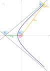 |
Fig. B.1 Schematics of a hyperbolic trajectory (dark blue line) for a coplanar fly-by viewed from above. The host star with a disk (indicated by the purple circle) is placed at the origin of the coordinate system. Black dotted lines indicate the asymptotes. |
The code FARGO3D takes the initial position and velocity vector as the fly-by object as input and integrates the trajectory using a fifth-order Runge-Kutta N-body solver. We therefore needed to calculate these quantities from the parameters of the hyperbola. For that, we fix the initial distance dini between the perturber and the disk hosting star (indicated in Figure B.1).
From this initial distance, we can calculate the initial true anomaly using the hyperbolic trajectory equation
![Mathematical equation: $\[\theta_{\mathrm{ta}, \mathrm{ini}}=\arccos \left(-\frac{1}{e}\left[\frac{b^2}{a ~d_{\mathrm{ini}}}+1\right]\right).\]$](/articles/aa/full_html/2026/04/aa57365-25/aa57365-25-eq8.png) (B.3)
(B.3)
For a coplanar fly-by, the plane of the trajectory coincides with the plane of the disk, which lies in the x-y-plane in our setup. In this case, the initial position can be calculated from the true anomaly with
![Mathematical equation: $\[x=-\cos \left(\theta_{\mathrm{ta}}\right) ~d_{\mathrm{ini}}, \qquad\qquad y=\sin \left(\theta_{\mathrm{ta}}\right) ~d_{\mathrm{ini}}, \qquad\qquad z=0.\]$](/articles/aa/full_html/2026/04/aa57365-25/aa57365-25-eq9.png) (B.4)
(B.4)
The initial velocity vector can be determined with the flight path angle φ:
![Mathematical equation: $\[\tan (\varphi)=\frac{e ~\sin \left(\theta_{\mathrm{ta}}\right)}{1+e ~\cos \left(\theta_{\mathrm{ta}}\right)},\]$](/articles/aa/full_html/2026/04/aa57365-25/aa57365-25-eq10.png) (B.5)
(B.5)
leading to the velocity components
![Mathematical equation: $\[v_x=-v_{\mathrm{abs}} ~\cos \left(\varphi-\theta_{\mathrm{ta}}+\pi / 2\right) \qquad\qquad v_y=-v_{\mathrm{abs}} ~\sin \left(\varphi-\theta_{\mathrm{ta}}+\pi / 2\right) \qquad\qquad v_z=0,\]$](/articles/aa/full_html/2026/04/aa57365-25/aa57365-25-eq11.png) (B.6)
(B.6)
where vabs is the absolute value of the velocity. The absolute value can be calculated using the vis-viva equation
![Mathematical equation: $\[v_{\mathrm{abs}}=\sqrt{\mu\left(\frac{2}{d_{\mathrm{ini}}}-\frac{1}{a}\right)},\]$](/articles/aa/full_html/2026/04/aa57365-25/aa57365-25-eq12.png) (B.7)
(B.7)
where μ = GMtot is the standard gravitational parameter with Mtot as sum of the mass of the fly-by object and the mass of the host star.
Inclined fly-by trajectories can then be achieved by rotating the original in-plane hyperbola according to the orbital elements.
To test the configuration of the trajectory, we performed a couple of test simulations with different trajectory configurations. Because we were mainly interested in the fly-by trajectory in these tests, we set the disk resolution very low, which speeds up the computation time. This is reasonable, as the N-body integrator of FARGO3D does not depend on the grid resolution for the disk. The resulting trajectory from FARGO3D perfectly matches the analytical solution of the hyperbola in all our test cases, which confirms that our implementation of the initial position and velocity works correctly.
Appendix C Further evaluation of the hydrodynamic models
C.1 Twist
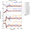 |
Fig. C.1 Precession angles for different radii in all four inclined simulations. The black dashed line indicates the precession angle for the total angular momentum vector of the disk. We only show times for where the inclination is ≥ 0.1°, as the precession angle is undefined otherwise. The blue and orange dashed lines highlight the times when the perturber crosses the initial disk midplane. For a good comparison, the range of the y-axis is the same in all panels. |
In addition to a warp, the disk can twist, a differential precession described analogously to Kimmig & Dullemond (2024) by the angle between the angular momentum vector of a disk annulus, projected to the x-y-plane, and the x-axis. Twists have been found to occur in fly-by scenarios, for example in Cuello et al. (2019). Figure D.2 shows the time evolution of the precession angle, p, which we calculated as the angle between the x-axis from the projection of the angular momentum vector to the x-y-plane:
![Mathematical equation: $\[p=\arctan \left(L_y, L_x\right),\]$](/articles/aa/full_html/2026/04/aa57365-25/aa57365-25-eq13.png) (C.1)
(C.1)
where Lx,y are the x, y-components of the angular momentum vector.
We find a differential precession, i.e., a twist, after the disk is warped, consistent with Kimmig & Dullemond (2024). This twist likely occurs due to pressure forces in the disk that influence the warp evolution. This is currently under investigation (Aly et al., in prep.). We note that the differential precession of the disk occurs on a full circular motion, even though Figure D.2 may suggest a motion rocking back and forth. This is due to our definition of the precession angle with respect to the static coordinate system instead of the precession axis. However, as the precession axis changes over time, there is no unambiguous definition for the precession motion, and we therefore decided to stay consistent with the definition of Kimmig & Dullemond (2024). Both prograde fly-bys show a more complicated pattern in the time between 0 − 500 yr, which is likely due to the spirals. If we compare Configuration 1 (with a periastron in plane) to Configuration 2, we see that the twist occurs slightly earlier for Configuration 2. This likely occurs because the perturber crosses the disk plane already prior to the periastron. To highlight this, we included the blue and orange dashed lines in Figure D.2. At these times, the gravitational force in vertical direction changes sign, leading to a strong perturbation. The twisting is strongest for the retrograde case of Configuration 2, where the warp is also strongest.
C.2 Disk truncation
Fly-bys are known to truncate the disk. We therefore briefly discuss this phenomenon in our simulations. Breslau et al. (2014) found an empirical relation of final disk sizes after a fly-by
![Mathematical equation: $\[r_{\text {final}} \approx 0.28 ~q^{-0.32} ~r_{\text {peri}},\]$](/articles/aa/full_html/2026/04/aa57365-25/aa57365-25-eq14.png) (C.2)
(C.2)
where q is the mass ratio between the two stars and rperi the distance of the closest approach. Disks experiencing a prograde fly-by are affected more strongly than retrograde fly-bys, where disks can be up to twice as large (Bhandare et al. 2016; Cuello et al. 2019).
In our simulations, q = 1 and rperi = 104 au, and therefore we would expect a disk size of 29 au. However, our disks are already compact from the beginning, with 26 au, and we therefore do not expect the fly-by to affect the size of the disk.
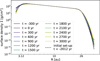 |
Fig. C.2 Evolution of the surface density in the retrograde simulation in Configuration 2. The time t = 0 yr corresponds to the time of closest approach. The black dashed line indicates the initial surface density setup according to Equation 1. |
Figure C.2 shows the surface density evolution for the retrograde Configuration 2 as an example. Indeed, the disk does not show truncation effects and only spreads slightly due to viscous evolution. We find this behavior in all of our simulations. This allowed us to keep the main focus on the warp evolution of the disks discussed above.
C.3 Spirals
Here, we present the spiral structure excited by the stellar fly-by in the prograde simulation of Configuration 2. In Figure C.3, we show the 2D surface density, which we obtain by vertically integrating the density in each radial shell. We show different snapshots within the lifetime of the spirals of about 500 yr, as suggested by Figure 8. We note that for more massive disks, the lifetime of the spirals could be prolonged if self-gravity becomes important (Papaloizou & Lin 1989).
In agreement with Smallwood et al. (2023), the pitch angle decreases over time as the spirals wind up. A detailed measurement of pitch angle and pattern speed is not trivial and would go beyond the scope of this work.
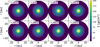 |
Fig. C.3 Snapshots of the simulation with an inclined prograde fly-by in Configuration 2 (periastron out of the disk plane). The closest approach occurs at t = 0 yr. The color scale for the surface density is linear, which highlights the spirals better than a logarithmic scale. |
Appendix D Parametric instability
Warped disks with low viscosity are suspected to be prone to the parametric instability (Gammie et al. 2000), which is a hydrodynamic instability that arises due to a parametric resonance of inertial waves and is enhanced by the free energy in oscillating shear flows. Such shear flows, often called sloshing and breathing motions, are known to occur in warped disks (see, e.g.,, Lubow & Ogilvie 2000; Ogilvie & Latter 2013a,b; Fairbairn & Ogilvie 2021a,b; Dullemond et al. 2022). Previous studies have shown that the parametric instability can operate already for small warp amplitudes and can enhance the dissipation of the warp (Deng et al. 2021; Fairbairn & Ogilvie 2023; Held & Ogilvie 2026). It is also known to operate in disks containing eccentricities (Ogilvie & Barker 2014; Dewberry et al. 2025). This parametric instability can enhance the dissipation of the warp amplitude.
We attempt to investigate if the parametric instability is operational in our simulations. For this, we continue to focus on the retrograde simulation in Configuration 2. We first transform the velocity field to a warped coordinate system, which aligns the midplane, meaning that the midplane is flat in these rotated coordinates. As the parametric instability is expected to be most prominent in the vertical velocity, we we focus on this velocity in a regime around the disk midplane. We note that we subtract the value of the vertical velocity of the midplane from the data, which is likely a motion of the disk plane arising from the warp evolution. In Section D.1, we verify that the resulting subtracted vertical velocity agrees with the expected vertical velocity from linear warp theory.
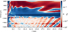 |
Fig. D.1 Radial profile of the vertical velocity at θ = 0.15 (at a specific azimuthal location) evolving over time (vertical axis). Time t = 0 yr indicates the point of closest approach of the fly-by. The vertical velocity is normalized by the maximum at each time step, similar to Fairbairn & Ogilvie 2023, Figure 10. We kept the rasterized grid appearance intentionally, as it highlights our resolution in space and time. |
We then plot the time evolution of the radial profile of one specific altitude (θ = 0.15 rad, ϕ = 0°) in Figure D.1. This representation of the vertical velocity is similar to Fairbairn & Ogilvie 2023, Figure 10, or Dewberry et al. 2025, for example Figure 4.
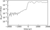 |
Fig. D.2 Warp amplitude ψ at r = 20 au in the disk. |
What is clearly visible in Figure D.1 is that the fly-by event adds strong distortions in the vertical directions that overpower any details that might result from the parametric instability. However, before the point of closest approach, structures appear similar to the results of Fairbairn & Ogilvie 2023, who investigated the parametric instability in detail on very small scales. Motivated by this, we evaluated the warp amplitude to estimate how much the disk is warped before the periastron of the perturber. The warp amplitude is defined by
![Mathematical equation: $\[\psi=\left|\frac{\mathrm{d} \boldsymbol{l}}{\mathrm{~d} ~\ln (r)}\right|,\]$](/articles/aa/full_html/2026/04/aa57365-25/aa57365-25-eq15.png) (D.1)
(D.1)
where l(r) is the local angular momentum vector.
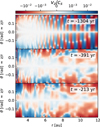 |
Fig. D.3 Cross-section of the vertical velocity vz scaled by the local sound speed cs at three different times before the moment of closest approach. The times are negative, as t = 0 yr. Note that this is zoomed in to the inner region of the disk r ≤ 12 au. |
Figure D.2 shows that the disk already slightly warps before the moment of closest approach (t = 0 yr) up to ψ = 10−3. This could already be enough to trigger the parametric instability (Fairbairn & Ogilvie 2023). We thus show the full vertical cross-sections of the vertical velocities at different times in Figure D.3.
Figure D.3 shows an oscillating vertical structure that resembles the structure found in a simulation by Deng et al. 2021 (see their Figure 6). In their work, they find indications that the parametric instability is at work in their simulations. This structure could be a signature of the parametric instability. However, our simulations do not contain enough resolution to resolve the very fine structure found by Fairbairn & Ogilvie 2023, and further, more detailed analysis and simulations with a much higher resolution would be required to strongly claim the presence of the parametric instability in our simulations.
Deng et al. 2021 find an increase in vertical kinetic energy in their simulations as an indication of the parametric instability. Evaluating the vertical kinetic energy in our simulations, we also find an increase. However, as our simulation includes an external perturber, the increase in vertical kinetic energy is connected to the perturber and therefore cannot straightforwardly be interpreted as a signature of the parametric instability.
D.1 Breathing motions
In this section, we take a closer look at the breathing motions occurring in the disk (Ogilvie & Latter 2013a; Fairbairn & Ogilvie 2021b). The purpose of this is mainly to verify our evaluation of the vertical velocity in Section D. We evaluate the retrograde simulation in Configuration 2 and aim to look at a stage when the disk is significantly warped. For that, we arbitrarily choose t = 320 yr after the closest approach. We present a cross-section through the vertical velocity in the rotated coordinate system in Figure D.4, left panel.
To investigate this pattern more closely, we compute the vertical velocity component vz = VzΩz according to linear analysis, given the exact warp shape at this snapshot of our simulation. Here, Vz is the velocity coefficient in the linear approximation as for example in Ogilvie & Latter 2013b and Dullemond et al. 2022. For details on the extraction of Vz from the 3D model, we refer the reader to Kimmig & Dullemond 2024, Appendix D. This reconstructed vertical velocity from linear theory is shown in Figure D.4, right panel. The two panels agree well in the regions close to the midplane, where the linear theory is applicable. We find some deviations at higher altitudes, especially close to the outer edge of the disk (rout = 26 au), which likely result from nonlinear effects in the 3D simulation.
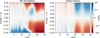 |
Fig. D.4 Cross-section of the velocity vz scaled by the local sound speed at t = 320 yr after the closest approach, shown in the rotated coordinate system. Left: velocity field in the 3D simulation, where the vertical velocity of the midplane is subtracted. Right: Reconstructed breathing motions from linear theory. |
Appendix E Calculation of the mutual geometry between orbit and disk
In this section, we derive the equations to find the mutual geometry of disk and orbit, in the case that the geometry of the disk plane and the orbit is given in the reference frame of the sky. We performed this consideration on the basis of the RW Aur geometry system, which is why we chose some definitions that are convenient for this specific case. However, this geometry consideration can be applied to other systems if careful attention is brought on these definitions. We define a left-handed coordinate system for the sky frame4, with the zsky-axis pointing away along the line of sight, as shown in Figure E.1.
An observed disk is characterized by a position angle Ωd, which corresponds to the longitude of ascending node in the plane of the sky, and an inclination θd with respect to the sky plane. From these angles, we can construct the normal vector of the disk in the reference frame of the sky
![Mathematical equation: $\[\boldsymbol{n}_{\mathbf{d}}=\left(\begin{array}{c}-\sin \left(\theta_{\mathrm{d}}\right) ~\cos \left(\Omega_{\mathrm{d}}\right) \\-\sin \left(\theta_{\mathrm{d}}\right) ~\sin \left(\Omega_{\mathrm{d}}\right) \\\cos \left(\theta_{\mathrm{d}}\right)\end{array}\right),\]$](/articles/aa/full_html/2026/04/aa57365-25/aa57365-25-eq16.png) (E.1)
(E.1)
where Ωd is the longitude of ascending node of the disk, corresponding to the crossing line of the disk with the plane of the sky. This angle is defined from North, or positive y-axis, as indicated in Figure E.1.
It is important to note that according to the geometry definition of trajectory to disk in Figure 1, the inclination angle θd is not the same angle as the inclination typically given in observations ![Mathematical equation: $\[\theta_{\mathrm{d}}^{\text {obs}}\]$](/articles/aa/full_html/2026/04/aa57365-25/aa57365-25-eq17.png) . This
. This ![Mathematical equation: $\[\theta_{\mathrm{d}}^{\text {obs}}\]$](/articles/aa/full_html/2026/04/aa57365-25/aa57365-25-eq18.png) is defined as the angle between the normal vector and the part of the line of sight pointing toward us (see Figure E.1). By this definition,
is defined as the angle between the normal vector and the part of the line of sight pointing toward us (see Figure E.1). By this definition, ![Mathematical equation: $\[\theta_{\mathrm{d}}=\pi-\theta_{\mathrm{d}}^{\text {obs }}\]$](/articles/aa/full_html/2026/04/aa57365-25/aa57365-25-eq19.png) . When we plug this into the normal vector in Equation E.1, with sin(π − θ) = sin(θ) and cos(π − θ) = − cos(θ) we see that the third component is negative for
. When we plug this into the normal vector in Equation E.1, with sin(π − θ) = sin(θ) and cos(π − θ) = − cos(θ) we see that the third component is negative for ![Mathematical equation: $\[\left|\theta_{\mathrm{d}}^{\text {obs }}\right|<\pi\]$](/articles/aa/full_html/2026/04/aa57365-25/aa57365-25-eq20.png) . This aligns with our definition of a left-handed coordinate system.
. This aligns with our definition of a left-handed coordinate system.
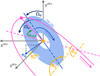 |
Fig. E.1 Geometry of the disk and fly-by orbit of the RW Aur system in the reference frame of the sky. Light blue indicates the disk, pink indicates the orbit, where the pink dashed line shows the crossing line of the plane of the orbit with the x-y-plane and the periastron (pink dot) is “in front,” meaning closer to us than the x-y-plane. The position angles Ωd,o, inclinations θd,o and the argument of the periapsis of the orbit ωo are defined consistently with our definition in Figure 1. Note that this coordinate system is left-handed. |
The orbit is characterized by a position angle Ωo, an inclination θo, and an argument of periapsis ωo. Here, the definition of inclination extracted from observations usually aligns with the inclination definition in Figure 1, which is why we can use the value from observations directly. The normal vector of the plane can be described analogously to the disk’s normal vector:
![Mathematical equation: $\[\boldsymbol{n}_{\mathbf{o}}=\left(\begin{array}{c}-\sin \left(\theta_{\mathrm{o}}\right) ~\cos \left(\Omega_{\mathrm{o}}\right) \\-\sin \left(\theta_{\mathrm{o}}\right) ~\sin \left(\Omega_{\mathrm{o}}\right) \\\cos \left(\theta_{\mathrm{o}}\right)\end{array}\right).\]$](/articles/aa/full_html/2026/04/aa57365-25/aa57365-25-eq21.png) (E.2)
(E.2)
E.1 Mutual inclination
The mutual inclination between the disk plane and the orbital plane then simply corresponds to the angle between the two normal vectors nd and no. This can be calculated by
![Mathematical equation: $\[\cos \left(\theta_{\mathrm{mut}}\right)=\frac{\boldsymbol{n}_{\mathrm{d}} \cdot \boldsymbol{n}_{\mathrm{o}}}{\left|\boldsymbol{n}_{\mathrm{d}}\right|\left|\boldsymbol{n}_{\mathrm{o}}\right|}=\boldsymbol{n}_{\mathrm{d}} \cdot \boldsymbol{n}_{\mathrm{o}},\]$](/articles/aa/full_html/2026/04/aa57365-25/aa57365-25-eq22.png) (E.3)
(E.3)
where the last term holds true because both vectors are unit vectors. This results in
![Mathematical equation: $\[\cos \left(\theta_{\mathrm{mut}}\right)=\sin \left(\theta_{\mathrm{d}}\right) ~\sin \left(\theta_{\mathrm{o}}\right) ~\cos \left(\Omega_{\mathrm{d}}-\Omega_{\mathrm{o}}\right)+\cos \left(\theta_{\mathrm{d}}\right) ~\cos \left(\theta_{\mathrm{o}}\right).\]$](/articles/aa/full_html/2026/04/aa57365-25/aa57365-25-eq23.png) (E.4)
(E.4)
The same expression can for example be found in van der Plas et al. (2019), their Equation 4 or Gonzalez et al. (2020), their Equation 2.
E.2 Argument of periapsis of the orbit with respect to the disk plane
Finding the argument of periapsis with respect to the disk plane is not trivial. Gonzalez et al. (2020) consider a similar geometric problem in the disk of HD 100453. However, in their SPH simulations, they were able to measure this angle. Here, we aim to derive an expression to calculate the angle from the given orientations of disk and orbit on the sky.
To derive the equation for this, we construct a vector along the longitude of ascending node of the orbit along the disk plane in the frame of the sky coordinate system, and a vector pointing to the periapsis. The argument of periapsis of the orbit with respect to the disk plane (which we call the mutual argument of periapsis in the following) then corresponds to the angle between those two constructed vectors.
First, we construct the vector along the longitude of ascending node of the orbit within the disk plane in the coordinate system of the sky. We call this vector d and calculate it with the cross product of the two normal vectors
![Mathematical equation: $\[\boldsymbol{d}^{\text {sky }}=\boldsymbol{n}_{\mathrm{d}} \times \boldsymbol{n}_{\mathrm{o}}=\left(\begin{array}{c}-\sin \left(\theta_{\mathrm{d}}\right) ~\sin \left(\Omega_{\mathrm{d}}\right) ~\cos \left(\theta_{\mathrm{o}}\right)+\cos \left(\theta_{\mathrm{d}}\right) ~\sin \left(\theta_{\mathrm{o}}\right) ~\sin \left(\Omega_{\mathrm{o}}\right) \\-\cos \left(\theta_{\mathrm{d}}\right) ~\sin \left(\theta_{\mathrm{o}}\right) ~\cos \left(\Omega_{\mathrm{o}}\right)+\sin \left(\theta_{\mathrm{d}}\right) ~\cos \left(\Omega_{\mathrm{d}}\right) ~\cos \left(\theta_{\mathrm{o}}\right) \\\sin \left(\theta_{\mathrm{d}}\right) ~\sin \left(\theta_{\mathrm{o}}\right) ~\sin \left(\Omega_{\mathrm{o}}-\Omega_{\mathrm{d}}\right)\end{array}\right).\]$](/articles/aa/full_html/2026/04/aa57365-25/aa57365-25-eq24.png) (E.5)
(E.5)
Second, we need to construct the vector pointing to the periapsis. For this, we define a new coordinate system in the plane of the orbit. We define it such that the periapsis lies on the ypf-axis. We use the index pf for this coordinate system, as it is sometimes called perifocal frame (see Figure E.2).
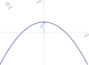 |
Fig. E.2 Our definition of the perifocal frame, which lies in the plane of the orbit. |
In this perifocal frame, the coordinates of the unit vector pointing to the periapsis are trivial: ppf = (0, 1, 0). To construct the coordinates of this vector in the reference frame of the sky, we need to rotate the coordinate system along all three angles that characterize the orientation of the orbit. As these characterizing angles are defined counter-clockwise, we need to rotate the coordinate system clockwise in order to find the correct coordinates. In a left-handed coordinate system, the following rotation matrices describe clockwise rotations:
![Mathematical equation: $\[R_\omega=\left(\begin{array}{ccc}\cos \left(\omega_{\mathrm{o}}\right) & -\sin \left(\omega_{\mathrm{o}}\right) & 0 \\\sin \left(\omega_{\mathrm{o}}\right) & \cos \left(\omega_{\mathrm{o}}\right) & 0 \\0 & 0 & 1\end{array}\right), \qquad R_\theta=\left(\begin{array}{ccc}\cos \left(\theta_{\mathrm{o}}\right) & 0 & \sin \left(\theta_{\mathrm{o}}\right) \\0 & 1 & 0 \\-\sin \left(\theta_{\mathrm{o}}\right) & 0 & \cos \left(\theta_{\mathrm{o}}\right)\end{array}\right), \quad \text { and } \qquad R_{\Omega}=\left(\begin{array}{ccc}\cos \left(\Omega_{\mathrm{o}}\right) & -\sin \left(\Omega_{\mathrm{o}}\right) & 0 \\\sin \left(\Omega_{\mathrm{o}}\right) & \cos \left(\Omega_{\mathrm{o}}\right) & 0 \\0 & 0 & 1\end{array}\right).\]$](/articles/aa/full_html/2026/04/aa57365-25/aa57365-25-eq25.png) (E.6)
(E.6)
Using these matrices, we can determine the coordinates of p in the frame of the sky:
![Mathematical equation: $\[\boldsymbol{p}^{\mathrm{sky}}=R_{\Omega} ~R_\theta ~R_\omega ~\boldsymbol{p}^{\mathrm{pf}}=\left(\begin{array}{c}-\cos \left(\Omega_{\mathrm{o}}\right) ~\cos \left(\theta_{\mathrm{o}}\right) \sin \left(\omega_{\mathrm{o}}\right)-\sin \left(\Omega_{\mathrm{o}}\right) ~\cos \left(\omega_{\mathrm{o}}\right) \\-\sin \left(\Omega_{\mathrm{o}}\right) ~\cos \left(\theta_{\mathrm{o}}\right) \sin \left(\omega_{\mathrm{o}}\right)+\cos \left(\Omega_{\mathrm{o}}\right) ~\cos \left(\omega_{\mathrm{o}}\right) \\\sin \left(\theta_{\mathrm{o}}\right) ~\sin \left(\omega_{\mathrm{o}}\right)\end{array}\right).\]$](/articles/aa/full_html/2026/04/aa57365-25/aa57365-25-eq26.png) (E.7)
(E.7)
We note that the rotations do not change the length of this vector, meaning that it still is a unit vector. With this, we can finally calculate the angle between dsky and psky, which gives the mutual argument of periapsis:
![Mathematical equation: $\[\cos \left(\omega_{\text {mut}}\right)=\boldsymbol{d}^{\text {sky}} \cdot \boldsymbol{p}^{\text {sky}}=\sin \left(\omega_{\mathrm{o}}\right) ~\sin \left(\theta_{\mathrm{d}}\right) ~\cos \left(2 \theta_{\mathrm{o}}\right) ~\sin \left(\Omega_{\mathrm{d}}-\Omega_{\mathrm{o}}\right)+\cos \left(\omega_{\mathrm{o}}\right)\left[\sin \left(\theta_{\mathrm{d}}\right) ~\cos \left(\theta_{\mathrm{o}}\right) \cos \left(\Omega_{\mathrm{o}}-\Omega_{\mathrm{d}}\right)-\cos \left(\theta_{\mathrm{d}}\right) ~\sin \left(\theta_{\mathrm{o}}\right)\right].\]$](/articles/aa/full_html/2026/04/aa57365-25/aa57365-25-eq27.png) (E.8)
(E.8)
Appendix F Further evaluation of the RW Aur models
F.1 Different disk viscosities
Because spirals might have different lifetimes for different disk viscosities, we investigate the hydrodynamical results in one simulation with a larger (α = 10−2) and one with a lower disk viscosity (α = 10−4). All other parameters, including the trajectory of the fly-by, remain exactly the same.
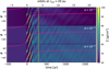 |
Fig. F.1 Azimuthal surface density profile evolution at r = 15 au for the simulations with different disk viscosities. The yellow dashed line indicates the current time and the pink line indicates the angle to the perturber. |
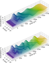 |
Fig. F.2 Evolution of the inclination profile in the simulation with α = 10−2 (top) and α = 10−4 (bottom). |
Figure F.1 shows the evolution of the azimuthal profile at r = 15 au for the simulations with different viscosities. The middle panel here shows the fiducial simulation presented before. The lifetime of the spirals does not depend strongly on the viscosity. As expected, the spirals dissolve slightly faster for higher viscosity. However, for lower viscosity, no significant difference in spiral lifetime is visible. This means that we do not expect to see strong spirals at the current time of observations, even if different assumptions on viscosity are taken. The lifetime of the spirals could, however, be dependent on other disk properties, such as initial disk size and vertical density structure (inter alia, flaring).
Investigating the warp in these simulations in Figure F.2, we find that the amplitude of the excited warp also does not depend on the disk viscosity. However, the viscosity influences the evolution of the warp after the fly-by. This is especially visible for the largest viscosity simulation as the warp is dampened rapidly. The two low-viscosity simulations show no strong differences on the short simulated timescales. However, we expect a longer lifetime of the warp for the lowest viscosity.
F.2 Additional radiative transfer data
Figure F.3 shows the convolved and unconvolved radiative transfer simulation in comparison to each other. In the unconvolved image, weak spiral structures close to the inner edge of the disk are visible. However, they disappear with the convolution.
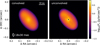 |
Fig. F.3 Similar to Figure 12, but both panels are the radiative transfer model. The left panel is convolved with a Gaussian beam, the right panel shows the unconvolved, raw output from the radiative transfer model. |
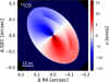 |
Fig. F.4 Velocity of the peak intensity of the initial setup of the hydrodynamic simulation of RW Aur A. We note that a part of the backside of the disk is visible at the near side of the disk in the upper right corner of the image. |
In Figure F.4, we show the velocity of the peak intensity we used to compute the residuals presented in Figure 16. We created this map using the initial setup of our hydrodynamic simulation of RW Aur A, which is a Keplerian disk model with corrections for pressure gradients.
Kur24 fit both the inner and outer disk freely. However, the outer disk inclination and position angle remain almost the same as for their original Markov chain Monte Carlo fitting.
The inner disk radius here is determined from near-IR observations and is closer in than the 3 au by Kur24.
Due to the definition of the angles as shown in Figure 1, we need to take the inclination θd, calc = 180° − θd, measured to calculate the mutual angles.
This left-handed coordinate system is motivated by the fact that East and West are typically flipped in observational coordinate systems.
All Tables
All Figures
|
Fig. 1 Schematics of the definition for the geometry of the fly-by trajectory with respect to the disk plane. Indicated are the inclination of the trajectory, θ; the longitude of the ascending node, Ω; and the argument of periapsis, ω. The distance of the closest approach (i.e., the periapsis) is rp. |
| In the text | |
|
Fig. 2 Trajectory configurations for our fly-by simulations. The disk lies in the x-y-plane at the origin of the coordinate system with a counter-clockwise rotation. Configuration 1 is shown in blue on the left, where the trajectory is rotated about the x-axis with a periapsis in the same plane as the disk. Configuration 2 (orange, right) is rotated about the y-axis with a periapsis out of the disk plane. |
| In the text | |
|
Fig. 3 Inclination evolution of the fly-by simulations with the prograde and retrograde fly-by of Configuration 1 (periastron in the same plane as the disk) in the top two panels and Configuration 2 (periastron out of disk plane) in the bottom two panels. Time t = 0 indicates the moment of closest approach. The color corresponds to time, and the blue and orange vertical dashed lines indicate the times when the perturber crosses the (initial) disk midplane. We note that we plot the inclination profile only up to the outer radius of the disk rout = 26 au, but the computational domain extends further out. |
| In the text | |
|
Fig. 4 Mean tilt defined as the angle between the total angular momentum vector of the disk and the z-axis for all six trajectory configurations. |
| In the text | |
|
Fig. 5 Evolution of the orbital plane at r = 23.9 au in the retrograde simulation in Configuration 2 (see Figure 2, right). We started the fit according to Equation (3) (blue dashed line) at the first maximum of the curve (dashed gray line) and stopped the fit at t = 1.58 × 10⁴ yr, where the period seems to change. We note that this figure shows the evolution over a longer time period than Figure 3. |
| In the text | |
|
Fig. 6 Surface density snapshots of the prograde fly-by in Configuration 2. Time t = 0 yr is the point of the closest approach. The gray dashed circle indicates a radius of 15 au, where we performed further analysis of the spirals. Further snapshots are shown in Appendix C.3. |
| In the text | |
|
Fig. 7 Time evolution of the peak surface density at r = 15 au in all six simulations. Prograde simulations are shown with solid lines, while retrograde simulations are indicated with dash-dotted lines. |
| In the text | |
|
Fig. 8 Azimuthal cut of the vertically integrated surface density at r = 15 au for all three prograde simulations. The pink line indicates the angle to the perturber projected to the x–y-plane. The time axis is scaled such that t = 0 yr indicates the point of the closest approach. |
| In the text | |
|
Fig. 9 Evolution of the inclination profile for the simulation of the disk around RW Aur A. The color indicates the time; time t = 0 indicates the point of the closest approach. |
| In the text | |
|
Fig. 10 Cross-section of the gas density in the model of RW Aur A at the current time (295 yr after periastron). |
| In the text | |
|
Fig. 11 Peak surface density (top panel) and azimuthal profile evolution (bottom panel) of the RW Aur simulation at r = 15 au. As in Figure 8, the pink line indicates the angle to the perturber. The dashed yellow line highlights the current point of time at t = 295 yr after periastron. |
| In the text | |
|
Fig. 12 Synthetic observation of our hydrodynamic simulation at t = 295 yr after periastron at a wavelength of λ = 1.3 mm (left panel) next to the ALMA Band 6 observation of RW Aur (right panel, Kurtovic et al. 2024), which is also at λ = 1.3 mm. The ellipse in the bottom-left corner indicates the beam and is the same for both images. |
| In the text | |
|
Fig. 13 Synthetic observations at λ = 1.3 mm of the RW Aur A simulation at different times. The first panel shows the initial setup of the simulation, time t = 0 yr is the time of the closest approach, and the current time step lies between the second last and last panels. The images were convolved with the same beam as Figure 12. |
| In the text | |
|
Fig. 14 Intensity of different velocity channels of the RW Aur A model at the current time of 295 yr after periastron passage. |
| In the text | |
|
Fig. 15 Moment 0 map (left) and velocity of the peak intensity (Moment 9, right) of the gas in the hydrodynamic model of the disk around RW Aur A at 295 yr after periastron. The line is centered at v = 0 km/s, which corresponds to proper motion corrected observations. |
| In the text | |
|
Fig. 16 Deviation from a Keplerian profile of the Moment 9 map shown in the right panel of Figure 15. |
| In the text | |
|
Fig. B.1 Schematics of a hyperbolic trajectory (dark blue line) for a coplanar fly-by viewed from above. The host star with a disk (indicated by the purple circle) is placed at the origin of the coordinate system. Black dotted lines indicate the asymptotes. |
| In the text | |
|
Fig. C.1 Precession angles for different radii in all four inclined simulations. The black dashed line indicates the precession angle for the total angular momentum vector of the disk. We only show times for where the inclination is ≥ 0.1°, as the precession angle is undefined otherwise. The blue and orange dashed lines highlight the times when the perturber crosses the initial disk midplane. For a good comparison, the range of the y-axis is the same in all panels. |
| In the text | |
|
Fig. C.2 Evolution of the surface density in the retrograde simulation in Configuration 2. The time t = 0 yr corresponds to the time of closest approach. The black dashed line indicates the initial surface density setup according to Equation 1. |
| In the text | |
|
Fig. C.3 Snapshots of the simulation with an inclined prograde fly-by in Configuration 2 (periastron out of the disk plane). The closest approach occurs at t = 0 yr. The color scale for the surface density is linear, which highlights the spirals better than a logarithmic scale. |
| In the text | |
|
Fig. D.1 Radial profile of the vertical velocity at θ = 0.15 (at a specific azimuthal location) evolving over time (vertical axis). Time t = 0 yr indicates the point of closest approach of the fly-by. The vertical velocity is normalized by the maximum at each time step, similar to Fairbairn & Ogilvie 2023, Figure 10. We kept the rasterized grid appearance intentionally, as it highlights our resolution in space and time. |
| In the text | |
|
Fig. D.2 Warp amplitude ψ at r = 20 au in the disk. |
| In the text | |
|
Fig. D.3 Cross-section of the vertical velocity vz scaled by the local sound speed cs at three different times before the moment of closest approach. The times are negative, as t = 0 yr. Note that this is zoomed in to the inner region of the disk r ≤ 12 au. |
| In the text | |
|
Fig. D.4 Cross-section of the velocity vz scaled by the local sound speed at t = 320 yr after the closest approach, shown in the rotated coordinate system. Left: velocity field in the 3D simulation, where the vertical velocity of the midplane is subtracted. Right: Reconstructed breathing motions from linear theory. |
| In the text | |
|
Fig. E.1 Geometry of the disk and fly-by orbit of the RW Aur system in the reference frame of the sky. Light blue indicates the disk, pink indicates the orbit, where the pink dashed line shows the crossing line of the plane of the orbit with the x-y-plane and the periastron (pink dot) is “in front,” meaning closer to us than the x-y-plane. The position angles Ωd,o, inclinations θd,o and the argument of the periapsis of the orbit ωo are defined consistently with our definition in Figure 1. Note that this coordinate system is left-handed. |
| In the text | |
|
Fig. E.2 Our definition of the perifocal frame, which lies in the plane of the orbit. |
| In the text | |
|
Fig. F.1 Azimuthal surface density profile evolution at r = 15 au for the simulations with different disk viscosities. The yellow dashed line indicates the current time and the pink line indicates the angle to the perturber. |
| In the text | |
|
Fig. F.2 Evolution of the inclination profile in the simulation with α = 10−2 (top) and α = 10−4 (bottom). |
| In the text | |
|
Fig. F.3 Similar to Figure 12, but both panels are the radiative transfer model. The left panel is convolved with a Gaussian beam, the right panel shows the unconvolved, raw output from the radiative transfer model. |
| In the text | |
|
Fig. F.4 Velocity of the peak intensity of the initial setup of the hydrodynamic simulation of RW Aur A. We note that a part of the backside of the disk is visible at the near side of the disk in the upper right corner of the image. |
| In the text | |
Current usage metrics show cumulative count of Article Views (full-text article views including HTML views, PDF and ePub downloads, according to the available data) and Abstracts Views on Vision4Press platform.
Data correspond to usage on the plateform after 2015. The current usage metrics is available 48-96 hours after online publication and is updated daily on week days.
Initial download of the metrics may take a while.