| Issue |
A&A
Volume 708, April 2026
|
|
|---|---|---|
| Article Number | A54 | |
| Number of page(s) | 13 | |
| Section | Extragalactic astronomy | |
| DOI | https://doi.org/10.1051/0004-6361/202557912 | |
| Published online | 25 March 2026 | |
Where giants dwell: Probing the environments of early massive quiescent galaxies
1
INAF – Astronomical Observatory of Trieste, via G.B. Tiepolo 11, I-34143, Trieste, Italy
2
IFPU – Institute for Fundamental Physics of the Universe, via Beirut 2, 34151, Trieste, Italy
3
Tianjin Normal University, Binshuixidao 393, 300387, Tianjin, People’s Republic of China
4
Institute for Physics, Laboratory for Galaxy Evolution, EPFL, Observatoire de Sauverny, Chemin Pegasi 51, 1290, Versoix, Switzerland
★ Corresponding author: This email address is being protected from spambots. You need JavaScript enabled to view it.
Received:
30
October
2025
Accepted:
11
February
2026
Abstract
We investigated the environments of massive quiescent galaxies at 3 ≲ z ≲ 5 using the GAlaxy Evolution and Assembly (GAEA) theoretical model. We selected galaxies with stellar mass above 1010.8 M⊙ and specific star formation rates below 0.3 × t−1+460Hubble, thus yielding a sample of about 5000 galaxies within a simulated volume of ∼685 Mpc. These galaxies have formation times that cover the range inferred from recent observational data well, including a few rare objects with very short formation timescales and early formation epochs. Model high-z quiescent galaxies are α-enhanced and exhibit a wide range of stellar metallicity, which is in broad agreement with current observational estimates. Massive high-z quiescent galaxies in our model occupy a wide range of environments, from void-like regions to dense knots at the intersections of filaments. Quiescent galaxies in under-dense regions typically reside in halos that collapsed early and grew rapidly at high redshift, though this trend becomes difficult to identify observationally due to large intrinsic scatter in star formation histories. The descendants of high-z massive quiescent galaxies display a broad distribution in mass and environment by z = 0, reflecting the stochastic nature of mergers. About one-third of these systems remain permanently quenched, while most rejuvenation events are merger-driven and more common in overdense regions. Our results highlight the diversity of early quiescent galaxies and caution against assuming that all such systems trace the progenitors of present day most massive clusters.
Key words: galaxies: abundances / galaxies: evolution / galaxies: formation / galaxies: high-redshift / galaxies: star formation / galaxies: stellar content
© The Authors 2026
 Open Access article, published by EDP Sciences, under the terms of the Creative Commons Attribution License (https://creativecommons.org/licenses/by/4.0), which permits unrestricted use, distribution, and reproduction in any medium, provided the original work is properly cited.
This article is published in open access under the Subscribe to Open model. This email address is being protected from spambots. You need JavaScript enabled to view it. to support open access publication.
1. Introduction
The assembly and quenching of massive galaxies are central questions in modern astrophysics. In the local Universe, where star formation can be measured accurately for large samples of galaxies using a variety of indicators, galaxies are found to follow a ‘bimodal’ distribution (e.g., Blanton et al. 2003; Kauffmann et al. 2003; Baldry et al. 2004). This bimodality exhibits a well-defined red sequence dominated by low star formation rates (SFRs), and a blue cloud populated by galaxies that are still actively forming stars at non-negligible rates. The wealth of observational information available in the local Universe has allowed us to characterize how the distribution in the specific SFR and/or color versus stellar mass plane depends on the environment, defined either in terms of local galaxy density or through a more “global” environmental proxy such as halo mass or large-scale overdensity. The fraction of passive galaxies is found to be larger in overdense regions (e.g., Kauffmann et al. 2004; Balogh et al. 2004; Baldry et al. 2006), indicating that environmental processes had a significant impact on at least a fraction of the quenched galaxy population observed today.
At earlier cosmic epochs, accurate measurements of the star formation are more difficult to obtain for statistical samples of galaxies, and a less accurate environmental characterization is typically possible due, for example, to only photometric redshift information being available or sparse spectroscopic sampling rates. Yet, available data lead to general trends that are similar to those observed in the local Universe, with an overall decrease of the fraction of quiescent galaxies at earlier cosmic epochs (Brammer et al. 2009; Whitaker et al. 2011; Muzzin et al. 2013; Weaver et al. 2023). The measured quiescent fractions remain very large among massive galaxies in clusters up to z ∼ 1 (e.g., Mei et al. 2009; van der Burg et al. 2020), and quiescent galaxies are still found in the cores of massive systems up to z ∼ 2, albeit with a relatively large cluster-to-cluster variation (Andreon et al. 2014; Strazzullo et al. 2019; Willis et al. 2020).
The recent advent of the James Webb Space Telescope (JWST) has significantly advanced our ability to identify and characterize quiescent galaxies at very early cosmic epochs. Thanks to its unprecedented sensitivity and resolution in the near- and mid-infrared, deep surveys such as the Cosmic Evolution Early Release Science programme (CEERS – Finkelstein et al. 2023) and the JWST Advanced Deep Extragalactic Survey (JADES – Eisenstein et al. 2023) have revealed a population of massive quiescent galaxies that significantly outnumber expectations from theoretical models (Carnall et al. 2023; Valentino et al. 2023; Baker et al. 2025a,b, and references therein). While the number of spectroscopically confirmed massive quiescent galaxies at early epochs increases steadily, their environments remain poorly constrained from an observational point of view. A few studies report evidence of galaxy overdensities around massive quiescent galaxies at z ≳ 3 (Kubo et al. 2021; McConachie et al. 2022; Ito et al. 2023; Jin et al. 2024), suggesting that at least a fraction of these can be found in overdense regions that potentially trace the earliest cluster progenitors. Given the challenges involved in a robust determination of the environment at these redshifts, it remains unclear if these few existing case studies are representative of the global population.
From a theoretical perspective, a strong correlation with environment would align with expectations from a biased hierarchical formation scenario in which early quenching preferentially occurs in the densest regions of the cosmic web. However, it remains an open question whether environmental processes are causally linked to quenching at these early times, or whether environment merely correlates with early halo collapse while internal mechanisms dominate the suppression of star formation. The latter scenario is more likely to apply to the most massive galaxies, which are expected to experience only internal physical processes for most of their lifetime (De Lucia et al. 2012).
A few recent studies have examined the environmental properties of quenched high-z massive galaxies within theoretical models of galaxy formation, and the results are somewhat contradictory. Kimmig et al. (2025) used the Magneticum Pathfinder1 simulation and find that the 36 quiescent galaxies with stellar masses larger than 3 × 10¹⁰ M⊙ identified at z ∼ 3.4 reside in underdense regions relative to galaxies of similar stellar mass. Kimmig et al. (2025) argued that, in the framework of the physical model implemented in Magneticum for feedback from stars and Active Galactic Nuclei (AGN), this is a consequence of more efficient gas ejection and lack of new gas replenishment in underdense regions. In contrast, Kurinchi-Vendhan et al. (2024, see also Weller et al. 2025), used the IllustrisTNG2 simulations and found that the ∼70 massive3 quiescent galaxies identified at z ∼ 3.7 in the TNG100 and TNG300 volumes are preferentially located in more massive halos and denser regions. These regions provide larger initial reservoirs of infalling gas, which promotes black hole (BH) mass growth and leads to quenching via AGN feedback4. Similar trends are reported in Szpila et al. (2025) for the SIMBA-C simulation. These studies suggest that investigating the environmental properties of massive quiescent galaxies at early cosmic epochs can offer valuable insights into their formation pathways, and into the physical processes shaping galaxy evolution in the early Universe.
In this study, we carried out a thorough study of the local and large-scale environment of massive quiescent galaxies at 3 < z < 5, taking advantage of our GAlaxy Evolution and Assembly (GAEA) model. This is a state-of-the-art theoretical model that includes an updated treatment for both stellar and AGN feedback and, as we have shown in previous work, reproduces the observed quiescent fractions as well as number densities of massive quiescent galaxies out to z ∼ 3 − 4. It therefore represents an ideal tool for the detailed study presented below. The layout of the paper is as follows. In Section 2, we introduce the GAEA model and the simulation used in this study. In Sections 3 and 4, we characterize the environment of high-z quiescent model galaxies, and in Section 5 we analyze to what extent the physical properties of high-z quiescent galaxies depend on their environment. In Section 6, we characterize the future evolution of galaxies in our model sample and its dependence on the environment. Finally, we summarize our results and give our conclusions in Section 7.
2. The simulation and the galaxy formation model
GAEA5 is a state-of-the-art theoretical model of galaxy formation that couples prescriptions for the evolution of different baryonic components with substructure-based merger trees extracted from high-resolution cosmological N-body simulations. The model builds on that presented in the original work by De Lucia & Blaizot (2007), but it has been updated significantly over the past few years. Topical developments include the following:
-
(i)
A detailed treatment of the non-instantaneous recycling of gas, energy, and metals, which enables the tracing of individual metal abundances (De Lucia et al. 2014).
-
(ii)
An updated parametrization of stellar feedback partially based on results from hydrodynamical simulations, tuned to reproduce the observed galaxy stellar mass function up to z ∼ 3 (Hirschmann et al. 2016)
-
(iii)
A treatment for partitioning the cold gaseous phase of model galaxies in its atomic and molecular components, tuned to reproduce the measured HI and H2 galaxy mass functions in the local Universe (Xie et al. 2017).
-
(iv)
A careful tracing of the angular momentum exchanges between different components, and a treatment for the non-instantaneous stripping of the cold and hot gaseous components associated with satellite galaxies (Xie et al. 2020).
-
(v)
An improved model for cold-gas accretion onto supermassive BHs and AGN driven outflows that is tuned to reproduce the measured evolution of the AGN luminosity function up to z ∼ 4 (Fontanot et al. 2020).
In previous works, we have shown that our model is able to reproduce a broad range of observational measurements including the observed multiphase gas content of central and satellite galaxies (Xie et al. 2020), the observed secondary dependence of the local galaxy mass–gas metallicity relation (De Lucia et al. 2020), and its evolution to higher redshift (Hirschmann et al. 2016; Fontanot et al. 2021). Notably for this work, the latest GAEA rendition (De Lucia et al. 2024; Xie et al. 2024) nicely reproduces the observed galaxy quenched fractions and the estimated number densities of massive quiescent galaxies (when accounting for cosmic variance) up to z ∼ 3 − 4. As discussed in De Lucia et al. (2024, see also De Lucia et al. 2025), GAEA also performs significantly better than other recently published theoretical models in reproducing the estimated quenched fractions in galaxy clusters at z ∼ 1.
The results presented in this paper are based on the Millennium Simulation (Springel et al. 2005). This simulation follows 21603 dark-matter particles in a cubic box of 500 Mpc h−1 on a side, and assumes cosmological parameters consistent with WMAP1 (ΩΛ = 0.75, Ωm = 0.25, Ωb = 0.045, n = 1, σ8 = 0.9, and H0 = 73 km s−1 Mpc−1). More recent estimations provide slightly different values for a few of these parameters, and in particular, a larger value for Ωm and a lower value for σ8. However, we do not expect these differences to significantly affect our model predictions; in fact, our recent work based on the P-Millennium Simulation (Fontanot et al. 2025) showed that results from the latest rendition of our model converge very well when run on different simulations from the Millennium suite (e.g., Wang et al. 2008; Guo et al. 2013).
For the analysis presented below, we selected massive quiescent galaxies at z ≳ 3.1 and z ≲ 5.3. Specifically, we considered all model galaxies in the redshift range of interest with stellar masses larger than 1010.8 M⊙6, after accounting for an observational uncertainty of 0.25 dex, and with a specific SFR lower than  , where tHubble is the age of the Universe at the corresponding redshift. We note that the assumed uncertainty is rather conservative at these redshifts and that a different selection would not change the results presented in this work qualitatively. Whenever appropriate, we discuss below how results depend on this convolution. We find a total of 4788 galaxies in the entire Millennium Simulation box satisfying these criteria. We did not prevent the descendant or progenitor of the same galaxies from being counted at different snapshots. About 87% of the selected galaxies are centrals, and about 7% are orphans; i.e., galaxies whose parent dark-matter substructure has been tidally stripped below the resolution limit of the simulation. In our model, these galaxies survive for a residual merger time before merging (this is justified by the fact that baryons are much more concentrated than dark matter). Since the number density of massive quiescent galaxies decreases rapidly with increasing redshift, the sample is dominated by galaxies at the lowest end of the redshift range considered: 2195 galaxies are found at z ∼ 3.1, 1287 at z ∼ 3.3, and 668 at z ∼ 3.6. There are only 12 massive quiescent galaxies at z ∼ 5.3 – the snapshot at the highest redshift considered.
As a point of comparison for part of the analysis presented below, we also considered a corresponding star forming sample, i.e., galaxies that are above the same stellar mass cut but have specific SFRs higher than the threshold assumed for quiescent galaxies. Our star forming sample is composed of 23 656 galaxies; ∼88% of these are centrals, and only ∼4% are orphans.
3. Possibility of the first quiescent galaxies sitting in the most massive halos
The first question we address relates to which halos host the most massive quiescent galaxies at z ≳ 3. The naive expectation (however, see discussion in Section 1) is that these galaxies can be considered as the signposts of significant overdensities in the early Universe, which might eventually collapse in the most massive systems at lower redshifts. However, the stellar-to-halo mass relation tends to be rather flat for halo masses larger than ∼ 1013 M⊙ (e.g. Girelli et al. 2020), suggesting that a broader distribution of halo masses should be expected. Figure 1 shows the correlation between galaxy stellar mass and parent halo mass for all model galaxies in our samples. Gray and cyan contours show the regions enclosing (from thicker to thinner lines) 30, 60, and 90% of the quiescent and star forming galaxies, respectively. To compute the distributions shown, we combined galaxies in the entire redshift range considered (3 ≲ z ≲ 5.3), but we verified that the trends were the same when considering narrower redshift bins. The figure shows that massive quiescent galaxies reside in halos that cover a broad range of masses, from Milky Way-like systems to the most massive systems that can be identified at these high redshifts. In this sense, they are not ‘special’ when compared to star forming galaxies of similar mass, that cover a similar range of parent halo masses. However, the distributions obtained for star forming galaxies tend to be shifted to lower halo masses with respect to those corresponding to quiescent galaxies, and the most massive halos tend to host primarily quiescent galaxies. This is in agreement with findings from Kurinchi-Vendhan et al. (2024) based on the IllustrisTNG simulation, and can be understood as a consequence of an accelerated growth of galaxies sitting at the center of very massive halos, and suppression of their star formation activity either because of mergers or because of AGN feedback. In our previous work, we showed that the dominant quenching channel for massive galaxies in GAEA is, in fact, AGN feedback (Xie et al. 2024). Similar conclusions have been reached by independent studies based on both hydro-dynamical simulations and semi-analytic models (Kurinchi-Vendhan et al. 2024; Szpila et al. 2025; Lagos et al. 2025), with the exception of the study by Kimmig et al. (2025) mentioned above and based on the Magneticum simulation.
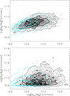 |
Fig. 1. Top panel: Relation between stellar mass and parent halo virial mass for all galaxies selected at z ≳ 3.1 and z ≲ 5.3 (trends are similar when considering galaxies in smaller redshift ranges). Gray and cyan contours show the regions enclosing (from thicker to thinner lines) 30, 60, and 90% of the quiescent and star forming galaxies, respectively. Bottom panel: same as above, but including an estimate of the observational uncertainty (0.25 dex) in the galaxy stellar mass. |
Figure 1 shows that there is a weak correlation between the intrinsic galaxy stellar mass and parent halo mass (top panel), both for quiescent and star forming massive galaxies. However, such a correlation is completely washed out when convolving the intrinsic galaxy mass with a (rather optimistic) estimate of the observational uncertainties (bottom panel). Being rather flat as a function of virial mass, the distributions shown in the bottom panel of Fig. 1 do not vary significantly when also including an estimate for the observational uncertainty on the parent halo’s mass.
Figure 2 shows, for all cosmic epochs considered, how the distributions of halo masses corresponding to the massive quiescent galaxies in our sample (solid lines) compare to the halo mass functions at the same cosmic epoch (dashed lines). Different colors correspond to different redshifts, from ∼3.1 (blue) to ∼5.3 (brown). The top and bottom panels are for all quiescent galaxies and for quiescent satellite galaxies in our sample, respectively. The figure confirms that, while the most massive halos at each cosmic epoch tend to host central quiescent galaxies, many central galaxies in halos more massive than ∼ 1013 M⊙ are forming stars at non-negligible rates and therefore are not counted in the solid histograms in the top panel of Fig. 2. The few satellite galaxies (∼620 out of 4788) in our sample do not exclusively reside in the most massive halos, but are distributed in the entire halo mass range covered by our sample. Combining the two panels, the figure also shows that the fraction of quiescent galaxies increases with halo mass, as observed at least in the local Universe (for a quantitative comparison between our model predictions and observational data, see De Lucia et al. 2019), and that this is not simply due to an increase of the satellite fraction.
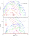 |
Fig. 2. Halo mass distribution for quiescent model galaxies (solid lines) and the corresponding halo mass function (dashed lines). Different colors correspond to different redshifts (as indicated in the legend in the bottom panel), ranging from ∼3.1 (blue) to ∼5.3 (brown). The top and bottom panels are for all quiescent galaxies and for quiescent satellites only, respectively. |
4. The environment of high-z quiescent galaxies
A measurement of parent halo mass is generally not easily accessible, in particular for the massive quiescent systems that are being observed at z > 3. In this section, we introduce different estimates that might be more easily obtained from observational data. In particular, for each galaxy in our sample, we computed the following:
-
(i)
-
A “local-density” estimate, corresponding to the density of galaxies inside the projected circular region enclosing the three closest neighbors. We refer to this density as n3 in the following.
-
(ii)
An “overdensity” estimate, corresponding to the mean overdensity of galaxies measured within a projected circular region of radius equal to 3 Mpc. This was normalized to the average value obtained at each redshift by randomly drawing 1000 spheres with radii equal to 3 Mpc in the entire volume of the simulation. We refer to this overdensity as o3 in the following.
In both cases, we considered projected physical distances and only galaxies within ∼20 Mpc depth slices and stellar masses larger than 109 M⊙. We verified that the results discussed below do not vary significantly when increasing the number of neighbors (up to 5 or 7) or the scale considered (we considered overdensities on scales of 5 and 8 Mpc).
For illustrative purposes, in Fig. 3 we show the projected spatial distribution of eight galaxies, all at z ∼ 4.5, from our sample of quiescent galaxies. The galaxies were selected to emphasize the variety of environments in which model high-z quiescent galaxies live. The top panels correspond to four galaxies in the lowest 15 percentiles of the distribution of the overdensities over 3 Mpc, while the bottom panels correspond to galaxies in the highest 85 percentiles of the same distribution. Selected galaxies are marked by a red cross and are shown at the center of the boxes, corresponding to a depth of 20 Mpc along the line of sight. We show the projected distribution of all galaxies more massive than 109 M⊙ at the same redshift; symbol size scales with galaxy stellar mass, while color scales with the galaxy SFR, as indicated by the color bars on the right of the figure. We note that we plot the most massive galaxies at the end, so they might hide smaller galaxies at close projected distances; this happens, for example, in the third panel in the bottom rom, where the massive quiescent galaxy at the center of the box is behind another massive star forming galaxy (see Figs. A.1 and A.2 in Appendix A for a similar plot, but only showing the distribution of the galaxies with low and high SFRs in the same regions). The mean overdensity, which is indicated in the top left corner of each box, increases from left to right in each row.
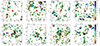 |
Fig. 3. Spatial distribution of galaxies selected at z ∼ 4.5 and with overdensities over a 3 Mpc scale in the lowest 15 (top panels) and highest 85 (bottom panels) percentiles of the distribution. Galaxies in our sample of massive quiescent galaxies are at the center of each panel and are marked by a red cross, while the other symbols mark the position of all galaxies more massive than 109 M⊙ in a projected region of 100 × 100 comoving Mpc, with a depth of 20 comoving Mpc. The o3 value corresponding to each field is indicated in the top left corner of each box. The color of the symbols scales with the galaxy SFR as indicated by the color bar on the right, while the symbol size scales with galaxy stellar mass. We note that we plot the most massive galaxies at the end to emphasize their position, so they may hide other galaxies that lie close in projection. |
Figure 3 shows that there is a wide range of environments in which early massive quiescent galaxies live, ranging from regions in which the closest massive galaxies reside at projected distances larger than ∼20 Mpc from the quiescent galaxy under consideration (top left panel) to regions with many other massive galaxies at relatively small projected distances from the target galaxy (e.g., first and third bottom panels). In a few cases, massive quiescent galaxies appear to reside on clear filamentary structures (e.g., third top panel), toward the center of a void-like structure (e.g., second top panel), or at the knot connecting different filaments (e.g., the bottom right panel; incidentally, this region contains two of the massive quiescent galaxies selected, the second being in the top right corner of the projected box). The SFRs of the galaxies residing in the projected regions considered ranges from very low levels consistent with zero to ∼ 250 M⊙ yr−1, with a non-negligible number of massive actively forming stars in each region (see Fig. A.2).
Although a direct comparison is difficult, the range of environments visible in Fig. 3 is much broader than that depicted in Fig. 4 of Remus & Kimmig (2025), showing the projected surface brightness of the gas at z = 3.4, with the position of the six most massive quiescent galaxies in the Magneticum Simulation Box3 superimposed. In this simulation, massive quiescent galaxies at high-z do inhabit different regions of the cosmic web, as is also in the case in our model, but none of them are found at the center (or close to the center) of the hottest regions (the most massive halos). As discussed in Section 1, this qualitative difference in the spatial distribution of massive quiescent galaxies is interesting because it suggests that it can be used, in principle, to constrain different physical mechanisms driving galaxy quenching at high z.
As discussed in previous work (Xie et al. 2024, see also Lagos et al. 2025), in our model the star formation in massive galaxies is suppressed by AGN-driven winds that are primarily driven by mergers. Fig. 4 shows the evolution of the parent halo mass, galaxy stellar mass, SFR, and BH mass for the same massive galaxies at z ∼ 4.5 considered in Fig. 3 (green and magenta lines are used for the lowest and highest percentiles of the o3 distribution, with line thickness and color shade increasing with increasing overdensity value). The figure shows that, already in this relatively small sample of galaxies, there is a large variety of evolutionary histories. The most massive galaxies do not necessarily reside in the most massive halos at the epoch of observation, as already discussed in the previous section, although the stellar mass assembly history parallels that of the parent dark-matter halos, as expected. The most striking trend as a function of overdensity is that galaxies residing in the least overdense regions tend to sit in halos that started growing earlier than their counterparts residing in regions that are overdense at the epoch of the observation. The earlier stellar and halo mass growth translates into an earlier growth of the BH mass that can lead to an earlier quenching of the star formation. Therefore, in this subsample of galaxies, lower overdensities are explained by an accelerated growth of halo and stellar mass before the epoch of the observations. It is important to stress that these galaxies were not selected randomly, but to emphasize the variety of the environments at these early cosmic epochs. We show later that the trend just discussed becomes insignificant when considering large samples of galaxies and large-scale overdensities as a proxy for the environment. However, it remains significant when considering local densities.
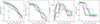 |
Fig. 4. Evolution of parent halo mass, galaxy stellar mass, SFR, and BH mass for the massive quiescent galaxies at z ∼ 4.5 considered in Fig. 3. Green and magenta lines refer to the top and bottom panels, respectively, with the thickness of the lines and color shade increasing with overdensity values as indicated in the legend included in the left panel. Different line styles are used to show different galaxies for clearer visualization. M200 and MBH are shown for the main progenitor at each previous cosmic epoch, while for the galaxy stellar mass and SFR we show the sum of all progenitors at the corresponding epoch. |
A more quantitative characterization of the environment of the quiescent galaxies in our sample is given in Fig. 5 showing the correlation between two different estimates of the galaxy environment and the parent halo mass (left column), the intrinsic galaxy stellar mass (middle column), and the same quantity convolved with an uncertainty of 0.25 dex (right column). The top panels correspond to the local density estimated considering the three closest neighbors for each model galaxy (n3), while the bottom panels correspond to an overdensity estimated over a 3 Mpc scale (o3). Black and cyan lines show the distributions for quiescent and star forming galaxies, respectively. The numbers in the top left and bottom right of each panel correspond to the Spearman correlation coefficient and relative significance (a small value indicates a significant correlation) for the two galaxy samples. The top left panel shows that there is a good although broad correlation between n3 and the parent halo mass, both for star forming and quiescent galaxies. A weak correlation is also visible between n3 and the intrinsic stellar mass (top middle panel); the most massive galaxies tend to have larger local densities, but the scatter is very large, and large values of n3 can be found for a quite broad range of galaxy stellar masses. This already weak correlation is almost entirely washed out when including an (optimistic) estimate of the uncertainty on the galaxy stellar mass (top right panel). The correlations with o3 are overall weaker, and an uncertainty regarding galaxy stellar mass can even invert the correlation with galaxy stellar mass (bottom right panel). The trends discussed here are very similar for quiescent and star forming galaxies, but for a small shift toward lower halo and stellar masses for the star forming galaxies. This shift appears to be more evident when considering local densities than larger scale overdensities. Results are qualitatively similar when considering local densities based on a larger number of neighbors or overdensities computed on larger scales.
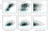 |
Fig. 5. Correlation between two different estimates of galaxy environment and the parent halo mass (left column), the intrinsic galaxy stellar mass (middle column), and the galaxy stellar mass including an estimate for its uncertainty (right column). The top panels are for n3, i.e., the local density (in physical Mpc−2) estimated considering the three closest neighbors for each galaxy in our quiescent (black) and star forming (cyan) samples. The bottom panels are for o3, i.e., the overdensity estimated considering a scale of 3 Mpc. The numbers in each panel correspond to the Spearman correlation coefficient and relative significance (a small value indicates a significant correlation) for quiescent galaxies (top left) and for star forming galaxies (bottom right). |
5. Physical properties of high-z quiescent galaxies depending on the environment
Having characterized the environments in which massive quiescent galaxies live, we can then ask to what extent their physical properties depend on their local or global environment. In this section, we focus on two different quantities for which observational measurements are rapidly being collected and/or will rapidly increase in the future: star formation histories and the stellar metallicities.
Galaxies in our sample of model quiescent systems are old, metal-rich, and α-enhanced. Figure 6 shows the distributions of the formation times, defined as the age of the Universe when half of the stellar mass had formed7, and the [O/Fe] abundances as a function of galaxy stellar mass. The color-coding indicates the redshift (as in Fig. 2). Open symbols with error bars in the top panel correspond to the observational estimates by Carnall et al. (2024) for five massive quiescent galaxies between z ∼ 3.2 and z ∼ 4.6. Filled symbols correspond to measurements by Nanayakkara et al. (2025) based on a sample of 19 quiescent galaxies with a median redshift of ∼3.55. For all these galaxies, JWST/NIRSpec spectroscopy is available. The two pairs of symbols connected by dashed lines correspond to the galaxies: ZF-UDS-6496 at z ∼ 4, with an estimated formation redshift of ∼5.6 in Carnall et al. (2024) and ∼5.9 in Nanayakkara et al. (2025); and ZF-UDS-7329 at z ∼ 3.2, with an estimated formation redshift of ∼11.2 in Carnall et al. (2024) and ∼8.8 in Nanayakkara et al. (2025). The range of estimated formation times for the same systems clearly shows the large systematic uncertainties, which are potentially more relevant than the reported statistical errors, associated with these measurements. One obvious source of systematic uncertainty is a different (e.g., more top-heavy) stellar initial mass function; this is something that we plan to address in future work.
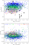 |
Fig. 6. Formation time (top panel) and [O/Fe] (bottom panel) as a function of galaxy stellar mass. The former is defined as the age of the Universe at which half of the stars in the galaxies were formed. Color coding is as a function of redshift, as indicated in the legend in the bottom panel. Open and filled symbols with error bars in the top panel correspond to observational measurements by Carnall et al. (2024, 5 galaxies between z ∼ 3.2 and z ∼ 4.6) and Nanayakkara et al. (2025, 19 galaxies with a median redshift of ∼3.55), respectively. Contours in the bottom panel show the regions enclosing (from thickest to thinnest) 30, 60, and 90% of the model sample. |
Our model predictions cover the entire range of formation times inferred from the data quite well. Note that in Fig. 6 we show the predicted intrinsic stellar masses on the x-axis to account for the better accuracy of the estimates based on spectroscopic information. However, even with spectroscopy, observational uncertainties are not negligible, and accounting for them would move many points to the right of the figure. At least a few would end up close to the massive galaxies in the observed sample with very high formation redshifts. The lower panel of Fig. 6 shows that all model quiescent galaxies in our sample are α-enhanced, with no significant trend as a function of stellar mass, but a trend as a function of redshift: quiescent galaxies identified at higher redshifts are more α-enhanced, as expected given the shorter formation times. To date, the only available measurement of α enhancement at these high redshifts was reported by Carnall et al. (2024); for the galaxy ZF-UDS-7329 at z ∼ 3.2, they reported a value of [Mg/Fe] =  . Considering an average positive offset of ∼0.10 − 0.15 between [O/Fe] and [Mg/Fe], this estimate is significantly higher than what is predicted for the bulk of our model galaxies at the same redshift, indicating that for most of the model galaxies star formation occurs over a longer timescale than inferred for this particular system. The relatively large uncertainties on these observational measurements ease concerns about the disagreement, and a top-heavy IMF would also lead to larger [α/Fe] ratios for model galaxies. In addition, we note that a few galaxies do exist in the simulated volume with intrinsic stellar masses larger than ∼ 1010.8 M⊙ and [O/Fe] larger than ∼0.40. Therefore, it is not impossible to have galaxies with properties similar to those inferred for ZF-UDS-7329 in the framework of our model.
Figure 7 shows the average star formation histories of the galaxies in our sample in the 25th (dark cyan) and 75th (dark magenta) percentiles of the distribution of n3. We omitted the very few galaxies in the highest redshift snapshots considered because of the low number statistics, and we matched8 the distributions of parent halo masses for the galaxies in the two extreme environments considered. The number of galaxies used at each redshift and for each environment bin is shown in the top left corner. The figure shows that there is a clear difference between galaxies residing in the regions corresponding to the highest and lowest values of n3. The trends reflect those described for Fig. 4: star formation tends to start earlier, proceed at faster rates, and decline earlier in regions corresponding to the lowest percentiles of the n3 distribution. No strong difference is observed for the timescale of quenching, which is very short in all cases (see Fig. 11 in Lagos et al. 2025). We verified that the differences evident in Fig. 7 are largely unaffected when considering local estimates based on a larger number of neighbors (n5 and n7). The different star formation histories corresponding to galaxies in regions with different (local) densities do not translate into a systematic difference in the ages of the stellar populations (when using the formation time as a proxy) of galaxies residing in these different environments. This is due to the very large scatter of the individual star formation histories as indicated by the thin lines (to avoid overcrowding the panels, we show a maximum of 50 randomly selected galaxies in each subsample at each redshift). We also verified that, when considering a global estimate of the environment, the differences between the median star formation histories corresponding to the two extremes is significantly reduced (see Fig. A.3 in Appendix A).
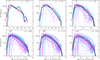 |
Fig. 7. Star formation histories of quiescent galaxies in the bottom 25 (cyan) and highest 75 (magenta) percentiles of the distribution of n3, considering matched distributions of parent halo mass. Thicker lines show the median star formation histories for each subsample. The numbers of galaxies in each subsample at each snapshot are given in the top left corner. A maximum of 50 individual star formation histories in each subsample are shown to avoid overcrowding the panels. |
Figure 8 shows the mass–metallicity relation for all quiescent galaxies in our sample, color-coded as a function of log(n3). In the top panel, the intrinsic galaxy stellar mass has been used, while in the bottom panel the galaxy stellar mass includes an uncertainty of 0.25 dex. The figure shows that there is a very weak trend with local density that is more evident for the galaxies with lowest masses in our sample; stellar metallicity is larger for galaxies in regions of lower local density as a consequence of the more prolonged star formation histories. However, this trend is completely washed out when an (optimistic) uncertainty on the galaxy stellar mass is included. We verified that no significant trend is visible in case a global density environment is considered. In absolute values, the available observational estimates of stellar metallicity reach larger values than those shown in Fig. 8, but they cover a wide range and are affected by large uncertainties: Nanayakkara et al. (2025) reported values of stellar metallicity ranging between ∼ − 0.55 and ∼0.54; for three of the galaxies in Carnall et al. (2024), the estimated metallicity is 0.32 − 0.35, while for the other two the estimated values are  and
and  . In fact, these measurements for high-redshift quiescent galaxies are very challenging because of the very weak metal absorption features due to young (in absolute terms) ages and the highly α-enhanced stellar populations. We refrained from adding observational estimates to Fig. 8 because of the very large estimated uncertainties, but note that model predictions also cover a wide range of metallicities.
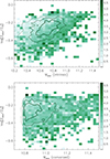 |
Fig. 8. Mass-(stellar)metallicity relation color-coded as a function of local density (n3). The upper panel shows the correlation between stellar metallicity and intrinsic galaxy stellar mass, while in the bottom panel model masses have been perturbed assuming an uncertainty of 0.25 dex on the galaxy mass. |
6. Descendants of early quiescent galaxies
One last question we can ask, taking advantage of our model results, is related to what the descendants of high-z quiescent galaxies are and if their future fate depends on the environments in which they reside. As noted above, about 88% of the galaxies selected at high z are centrals. Tracing their descendants down to z = 0, we find that about 77% are still centrals, while about 11% are orphans. Fig. 9 shows the distribution of parent halo mass (top panel) and stellar mass (middle panel), both for the galaxies selected at high redshifts (solid lines) and their descendants at z = 0 (dashed histograms). The purple and cyan lines correspond to the galaxies that are at two extremes in terms of percentiles (15th and 85th) of the distribution of o3 at high z. The bottom panel shows the correlation between the parent halo mass at z = 0 and the overdensity of o3 at the time of observation. The figure clearly shows that the distributions of halo masses and stellar masses of the z = 0 descendants of high-z quiescent galaxies are very broad, broader than the distribution found at the redshift of observation. This can be understood as a natural consequence of the stochasticity of merger events. The effect, which is stronger the higher the redshift, has been noted in earlier works and recognized as a generic prediction of hierarchical growth (e.g., De Lucia & Blaizot 2007; Trenti et al. 2008; Angulo et al. 2012). Fig. 9 also shows that the large-scale overdensity has a significant impact on the fate of the high-z quiescent galaxies; galaxies that are sitting in the largest overdensities are more likely be in a massive cluster today. There is a clear and rather strong correlation between the overdensity at the time of the observation and the halo mass at z = 0, which makes the latter a good predictor of the environment in which the descendants of high-z passive galaxies live at present. A clear but less significant difference appears when considering a local estimate of the environment. The latter is a more powerful indicator of the halo mass at the redshift of observations, but a less powerful indicator of the z = 0 halo mass (see Fig. A.4 in Appendix A). Similar results have been found in the recent work by Remus & Kimmig (2025). Their Fig. 15 shows a broad correlation between more dense environments at z = 3.4 and larger z = 0 halo masses. However, 75% of their high-z quiescent galaxies lie in underdense environments according to their definition. As noted above, this is likely related to how AGN feedback was implemented in their simulation, and it is worth noting that their particular implementation of stellar and AGN feedback does not lead to a good agreement with the observed evolution of the galaxy stellar mass function at lower redshifts (Hirschmann et al. 2014; Steinborn et al. 2015).
 |
Fig. 9. Solid histograms show the distribution of parent halo mass (top panel) and stellar mass (middle panel) for all quiescent model galaxies. Dashed histograms are the corresponding distributions for their descendants at z = 0. Cyan and magenta are used for galaxies that are in the extremes (15th and 85th percentiles) of the distribution of o3. The bottom panel shows the correlation between the virial mass of the halos in which descendants of galaxies in our sample reside at z = 0 and the overdensity at the time of the observation. Contours in the bottom panel show the regions enclosing (from thicker to thinner) 30, 60, and 90% of the galaxies. |
A more detailed characterization of the future star formation history of high-z quiescent galaxies is shown in Fig. 10. For each model galaxy, we followed the descendant to z = 0 and identified all snapshots where the specific SFR is above the threshold used to identify a galaxy as quiescent ( – see Section 2). We merged adjacent snapshots when counting these “rejuvenation” episodes. The top panels of Fig. 10 show the distributions of the number of rejuvenation episodes, the SFR during each episode, and the associated timescale. The bottom panels show the distributions of the total number of mergers in the last snapshot just before the rejuvenation episodes, the number of mergers with a mass ratio of at least 1/10, and the associated increase of stellar mass (excluding the stellar mass that is accreted through mergers). Magenta and cyan lines are for the 15th and 85th percentiles of the o3 distributions, as in previous figures.
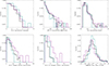 |
Fig. 10. Top panels: Distributions of the number of rejuvenation episodes, of the SFR during each episode, and of the associated timescale. Bottom panels: Distributions of the total number of mergers in the last snapshot just before the rejuvenation episodes, of the number of mergers with a mass ratio of at least 1/10, and of the associated fractional increase of stellar mass (excluding the stellar mass that is accreted through mergers). Magenta and cyan are for the 15th and 85th percentiles of the o3 distributions. |
In the framework of our model, rejuvenation is not a common event in the future lifetime of a massive quiescent galaxy at high z. About 36% of the quiescent galaxies in the selected sample remain passive down to z = 0, experiencing no rejuvenation events. For the rest of the galaxies in the sample, the mean number of rejuvenation episodes is ∼1.6 (with a median number of 1). Only very few galaxies experience more than four rejuvenation episodes (15 galaxies in total out of 4788). The overall fraction of galaxies experiencing rejuvenation in our model is larger than that quoted in Szpila et al. (2025), but very close to that estimated in Remus & Kimmig (2025). However, we note that these numbers are very sensitive to the exact definitions adopted. The galaxies with more frequent episodes of rejuvenation events tend to reside in the less overdense regions at the time of observations, but the number statistics are very low.
About 34% of the rejuvenation episodes are associated with a SFR lower than 10 M⊙ yr−1, but ∼5% of the galaxies in our sample have rejuvenation episodes with associated rates over 100 M⊙ yr−1. A larger number of these episodes are associated with galaxies that reside in the overdense regions at the epoch of observations. The vast majority of the rejuvenation episodes correspond to events occurring over only one snapshot of the simulation; the interval between subsequent snapshots varies between ∼110 and ∼270 Myr at z ∼ 5 and z = 0, respectively. Only a few episodes last much longer; i.e., the galaxy accretes significant amounts of gas to sustain star formation over several snapshots. Rejuvenation episodes are typically associated with recent mergers. A few of the galaxies in our sample experience a relatively large number of mergers, but many of these have very low mass ratios (see bottom left and bottom middle panels). For about 15% of the galaxies in the sample, the increase in mass associated with the rejuvenation episodes (subtracting the mass accreted through mergers) is non-negligible (larger than 1010 M⊙). The fractional mass increase with respect to the present stellar mass tends to be larger for galaxies in underdense environments (bottom right panel), due to the large difference between the present-day stellar mass of galaxies residing in overdense and underdense environments (see middle panel of Fig. 9).
7. Summary and conclusions
In this work, we analyzed the environment of massive quiescent galaxies at 3 ≲ z ≲ 5 using our GAEA theoretical model of galaxy formation. We selected galaxies with stellar masses larger than 1010.8 M⊙ and specific SFRs below  , resulting in a sample of about 5000 galaxies within a cubic simulated volume of ∼685 Mpc comoving on one side. In previous work, we showed that the latest rendition of our model reproduces a wide range of observational results, including the observed quiescent fractions and number densities up to z ∼ 3 − 4, providing an ideal tool for the analysis presented in this paper. We show that the formation times derived for model galaxies at z ≳ 3 cover the range inferred from recent observational work well (Carnall et al. 2024; Nanayakkara et al. 2025). Galaxies with very short formation timescales and early formation epochs are present in our model, though they are rare. Systems such as ZF-UDS-7329 are therefore not impossible in the framework of our model, though their true abundance in the Universe remains uncertain.
Model high-z quiescent galaxies are α-enhanced and exhibit a wide range of stellar metallicity broadly consistent with observational trends, though they do not reach the highest metallicities recently inferred. These measurements remain challenging due to the weakness of diagnostic spectral lines and the lack of well-tested, α-enhanced stellar population models for young (≲1 Gyr) ages. More accurate observational constraints will be essential for using these chemical signatures to test and refine our current galaxy formation model.
Our main conclusions are summarised below.
(i) Environmental diversity: massive quiescent high-z galaxies inhabit a wide range of environments, spanning from underdense regions resembling voids, to filaments, walls, and dense knots at the intersections of filaments. Their environment, whether characterized by halo mass, local neighbor counts, or large-scale overdensity, are far from uniform.
(ii) Environmental trends and halo history: quiescent galaxies that live in underdense regions at the epochs of the observation tend to reside in halos that collapsed earlier and experienced rapid early growth. This trend is most evident when considering a local estimate for the environment, and it becomes less clear when using large-scale overdensity. In addition, these correlations can be diluted or even inverted if halo mass is not controlled, making their observational detection challenging given current uncertainties and the intrinsic large scatter in star formation histories.
(iii) Descendant diversity: the descendants of high-z massive quiescent galaxies span a broad range of halo and stellar masses by z = 0 due to the stochastic nature of mergers. Some galaxies evolve little and remain in group-sized halos, while others grow significantly and end up in cluster-sized halos by z = 0. The large-scale overdensity measured at the epoch of the observations serves as a useful, though not perfect, predictor of the descendant halo mass at z = 0.
(iv) Rejuvenation: about 36% of the massive quiescent galaxies in our sample do not experience any subsequent rejuvenation, and only a few galaxies undergo multiple (> 4) rejuvenation events accompanied by strong bursts of star formation. Most rejuvenation episodes are merger-driven and occur more frequently in overdense environments at the epoch of observation.
These findings have important implications for current and future observational programs aimed at using environmental diagnostics to test quenching mechanisms or to identify the progenitors of present-day massive clusters. Both the number densities and environmental properties of massive quiescent galaxies at z ≳ 3 are expected to exhibit significant cosmic variance. Furthermore, such galaxies do not necessarily reside in the most massive halos of their epoch, nor do they always trace the sites that will evolve into the most massive clusters by z = 0. This is only partly due to uncertainties in stellar mass estimates and largely reflects the stochastic nature of mass accretion, as discussed in previous work (e.g., De Lucia & Blaizot 2007; Trenti et al. 2008; Overzier et al. 2009; Angulo et al. 2012, see also Fontanot et al. in preparation).
Acknowledgments
We acknowledge the use of INAF-OATs computational resources within the framework of the CHIPP project (Taffoni et al. 2020). MH acknowledges funding from the Swiss National Science Foundation (SNSF) via a PRIMA grant PR00P2-193577 ‘From cosmic dawn to high noon: the role of BHs for young galaxies’.
References
- Andreon, S., Newman, A. B., Trinchieri, G., et al. 2014, A&A, 565, A120 [NASA ADS] [CrossRef] [EDP Sciences] [Google Scholar]
- Angulo, R. E., Springel, V., White, S. D. M., et al. 2012, MNRAS, 425, 2722 [NASA ADS] [CrossRef] [Google Scholar]
- Baker, W. M., Lim, S., D’Eugenio, F., et al. 2025a, MNRAS, 539, 557 [Google Scholar]
- Baker, W. M., Valentino, F., Lagos, C. d. P., et al. 2025b, arXiv e-prints [arXiv:2506.04119] [Google Scholar]
- Baldry, I. K., Glazebrook, K., Brinkmann, J., et al. 2004, ApJ, 600, 681 [Google Scholar]
- Baldry, I. K., Balogh, M. L., Bower, R. G., et al. 2006, MNRAS, 373, 469 [Google Scholar]
- Balogh, M. L., Baldry, I. K., Nichol, R., et al. 2004, ApJ, 615, L101 [Google Scholar]
- Blanton, M. R., Hogg, D. W., Bahcall, N. A., et al. 2003, ApJ, 594, 186 [NASA ADS] [CrossRef] [Google Scholar]
- Brammer, G. B., Whitaker, K. E., van Dokkum, P. G., et al. 2009, ApJ, 706, L173 [Google Scholar]
- Carnall, A. C., McLeod, D. J., McLure, R. J., et al. 2023, MNRAS, 520, 3974 [NASA ADS] [CrossRef] [Google Scholar]
- Carnall, A. C., Cullen, F., McLure, R. J., et al. 2024, MNRAS, 534, 325 [NASA ADS] [CrossRef] [Google Scholar]
- De Lucia, G., & Blaizot, J. 2007, MNRAS, 375, 2 [Google Scholar]
- De Lucia, G., Weinmann, S., Poggianti, B. M., Aragón-Salamanca, A., & Zaritsky, D. 2012, MNRAS, 423, 1277 [NASA ADS] [CrossRef] [Google Scholar]
- De Lucia, G., Tornatore, L., Frenk, C. S., et al. 2014, MNRAS, 445, 970 [Google Scholar]
- De Lucia, G., Hirschmann, M., & Fontanot, F. 2019, MNRAS, 482, 5041 [Google Scholar]
- De Lucia, G., Xie, L., Fontanot, F., & Hirschmann, M. 2020, MNRAS, 498, 3215 [NASA ADS] [CrossRef] [Google Scholar]
- De Lucia, G., Fontanot, F., Xie, L., & Hirschmann, M. 2024, A&A, 687, A68 [NASA ADS] [CrossRef] [EDP Sciences] [Google Scholar]
- De Lucia, G., Fontanot, F., Hirschmann, M., & Xie, L. 2025, arXiv e-prints [arXiv:2502.01724] [Google Scholar]
- Eisenstein, D. J., Willott, C., Alberts, S., et al. 2023, arXiv e-prints [arXiv:2306.02465] [Google Scholar]
- Finkelstein, S. L., Bagley, M. B., Ferguson, H. C., et al. 2023, ApJ, 946, L13 [NASA ADS] [CrossRef] [Google Scholar]
- Fontanot, F., De Lucia, G., Hirschmann, M., et al. 2020, MNRAS, 496, 3943 [CrossRef] [Google Scholar]
- Fontanot, F., Calabrò, A., Talia, M., et al. 2021, MNRAS, 504, 4481 [CrossRef] [Google Scholar]
- Fontanot, F., De Lucia, G., Xie, L., et al. 2025, A&A, 699, A108 [NASA ADS] [CrossRef] [EDP Sciences] [Google Scholar]
- Girelli, G., Pozzetti, L., Bolzonella, M., et al. 2020, A&A, 634, A135 [NASA ADS] [CrossRef] [EDP Sciences] [Google Scholar]
- Guo, Q., White, S., Angulo, R. E., et al. 2013, MNRAS, 428, 1351 [NASA ADS] [CrossRef] [Google Scholar]
- Hirschmann, M., Dolag, K., Saro, A., et al. 2014, MNRAS, 442, 2304 [Google Scholar]
- Hirschmann, M., De Lucia, G., & Fontanot, F. 2016, MNRAS, 461, 1760 [Google Scholar]
- Ito, K., Tanaka, M., Valentino, F., et al. 2023, ApJ, 945, L9 [NASA ADS] [CrossRef] [Google Scholar]
- Jin, S., Sillassen, N. B., Magdis, G. E., et al. 2024, A&A, 683, L4 [NASA ADS] [CrossRef] [EDP Sciences] [Google Scholar]
- Kauffmann, G., Heckman, T. M., White, S. D. M., et al. 2003, MNRAS, 341, 33 [Google Scholar]
- Kauffmann, G., White, S. D. M., Heckman, T. M., et al. 2004, MNRAS, 353, 713 [Google Scholar]
- Kimmig, L. C., Remus, R.-S., Seidel, B., et al. 2025, ApJ, 979, 15 [Google Scholar]
- Kubo, M., Umehata, H., Matsuda, Y., et al. 2021, ApJ, 919, 6 [NASA ADS] [CrossRef] [Google Scholar]
- Kurinchi-Vendhan, S., Farcy, M., Hirschmann, M., & Valentino, F. 2024, MNRAS, 534, 3974 [NASA ADS] [CrossRef] [Google Scholar]
- Lagos, C. d. P., Valentino, F., Wright, R. J., et al. 2025, MNRAS, 536, 2324 [Google Scholar]
- McConachie, I., Wilson, G., Forrest, B., et al. 2022, ApJ, 926, 37 [NASA ADS] [CrossRef] [Google Scholar]
- Mei, S., Holden, B. P., Blakeslee, J. P., et al. 2009, ApJ, 690, 42 [NASA ADS] [CrossRef] [Google Scholar]
- Muzzin, A., Marchesini, D., Stefanon, M., et al. 2013, ApJ, 777, 18 [NASA ADS] [CrossRef] [Google Scholar]
- Nanayakkara, T., Glazebrook, K., Schreiber, C., et al. 2025, ApJ, 981, 78 [Google Scholar]
- Overzier, R. A., Guo, Q., Kauffmann, G., et al. 2009, MNRAS, 394, 577 [NASA ADS] [CrossRef] [Google Scholar]
- Remus, R.-S., & Kimmig, L. C. 2025, ApJ, 982, 30 [Google Scholar]
- Springel, V., White, S. D. M., Jenkins, A., et al. 2005, Nature, 435, 629 [Google Scholar]
- Steinborn, L. K., Dolag, K., Hirschmann, M., Prieto, M. A., & Remus, R.-S. 2015, MNRAS, 448, 1504 [Google Scholar]
- Strazzullo, V., Pannella, M., Mohr, J. J., et al. 2019, A&A, 622, A117 [NASA ADS] [CrossRef] [EDP Sciences] [Google Scholar]
- Szpila, J., Davé, R., Rennehan, D., Cui, W., & Hough, R. T. 2025, MNRAS, 537, 1849 [Google Scholar]
- Taffoni, G., Becciani, U., Garilli, B., et al. 2020, in Astronomical Data Analysis Software and Systems XXIX, eds. R. Pizzo, E. R. Deul, J. D. Mol, J. de Plaa, & H. Verkouter, ASP Conf. Ser., 527, 307 [NASA ADS] [Google Scholar]
- Trenti, M., Santos, M. R., & Stiavelli, M. 2008, ApJ, 687, 1 [Google Scholar]
- Valentino, F., Brammer, G., Gould, K. M. L., et al. 2023, ApJ, 947, 20 [NASA ADS] [CrossRef] [Google Scholar]
- van der Burg, R. F. J., Rudnick, G., Balogh, M. L., et al. 2020, A&A, 638, A112 [NASA ADS] [CrossRef] [EDP Sciences] [Google Scholar]
- Wang, J., De Lucia, G., Kitzbichler, M. G., & White, S. D. M. 2008, MNRAS, 384, 1301 [CrossRef] [Google Scholar]
- Weaver, J. R., Davidzon, I., Toft, S., et al. 2023, A&A, 677, A184 [NASA ADS] [CrossRef] [EDP Sciences] [Google Scholar]
- Weller, E. J., Pacucci, F., Ni, Y., Hernquist, L., & Park, M. 2025, ApJ, 979, 181 [Google Scholar]
- Whitaker, K. E., Labbé, I., van Dokkum, P. G., et al. 2011, ApJ, 735, 86 [Google Scholar]
- Willis, J. P., Canning, R. E. A., Noordeh, E. S., et al. 2020, Nature, 577, 39 [NASA ADS] [CrossRef] [Google Scholar]
- Xie, L., De Lucia, G., Hirschmann, M., Fontanot, F., & Zoldan, A. 2017, MNRAS, 469, 968 [Google Scholar]
- Xie, L., De Lucia, G., Hirschmann, M., & Fontanot, F. 2020, MNRAS, 498, 4327 [NASA ADS] [CrossRef] [Google Scholar]
- Xie, L., De Lucia, G., Fontanot, F., et al. 2024, ApJ, 966, L2 [NASA ADS] [CrossRef] [Google Scholar]
They only selected galaxies with stellar mass larger than 1010.6 M⊙.
It is the radiatively inefficient regime that leads, in the framework of this model, to an efficient momentum injection by AGN feedback. TNG assumes a switch from the radiatively efficient to the inefficient mode that depends on the BH mass. Therefore, the faster BH growth, promoted in overdense regions, leads to earlier gas accretion in the inefficient regime.
Details about the model and access to a selection of data products can be found at: https://sites.google.com/inaf.it/gaea/.
The stellar mass cut adopted is rather arbitrary, and it represents a compromise between the large estimated stellar mass quoted in recent observational studies (e.g., Carnall et al. 2024) and the goal of having a large enough statistical sample of model galaxies.
For our model galaxies, this is computed by linearly interpolating the predicted stellar mass at the outputs available.
Due to the significant correlation between n3 and halo mass (top left panel of Fig. 5), there is still a small yet systematic difference between the median halo mass in the two distributions of ∼0.1 dex.
Appendix A: Additional figures
Figs. A.1 and A.2 show the projected positions of galaxies with SFRs lower than ∼ 5 M⊙ yr−1 and larger than ∼ 80 M⊙ yr−1, respectively. The boxes correspond to those in Fig. 3, with gray symbols showing all galaxies with stellar mass larger than 109 M⊙ independently of their SFR. A certain number of galaxies forming stars at large rates can be found in all boxes considered. In most cases these tend to avoid the central regions of the boxes but in a few cases, due to projection effects and to the large projected volumes shown, they appear to lie very close to the central regions.
Fig. A.3 is the equivalent of Fig. 7 but showing the average star formation histories of galaxies in our quiescent sample in the 25th (dark cyan) and 75th (dark magenta) percentiles of the distribution of o3. While there is a clear different (albeit with a very large scatter) between the extremes considering the n3 distribution as discussed in the main body of the paper, this difference is largely removed when considering larger scale overdensities.
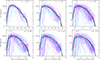 |
Fig. A.3. The star formation histories of galaxies in the bottom 25th (cyan) and highest 75th (magenta) percentiles of the distribution of o3. Ticker lines show the median star formation histories. The numbers of galaxies in each sub-sample at each snapshot is given in the top left corner. A maximum of 50 individual star formation histories in each subsample is shown to avoid overcrowding the panels. |
Fig. A.4 is the equivalent of Fig. 9 but for galaxies in the extremes of the n3 distribution. The figure shows that n3 is a less powerful indicator of the z = 0 halo mass: the scatter shown in the bottom panel is significantly larger than that discussed in Sec. 6 when considering o3. However, the correlation is still present so that galaxies in the extreme of the distribution still have offsetted distributions of virial mass and stellar mass, as shown in the top and middle panels.
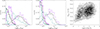 |
Fig. A.4. As in Fig. 9, but cyan and magenta histograms in the top and middle panel corresponds to galaxies in the extreme of the n3 distribution. The bottom panel shows the correlation between the halo mass in which descendants of quiescent high-z galaxies reside at z = 0 and n3 at the time of observation. |
All Figures
|
Fig. 1. Top panel: Relation between stellar mass and parent halo virial mass for all galaxies selected at z ≳ 3.1 and z ≲ 5.3 (trends are similar when considering galaxies in smaller redshift ranges). Gray and cyan contours show the regions enclosing (from thicker to thinner lines) 30, 60, and 90% of the quiescent and star forming galaxies, respectively. Bottom panel: same as above, but including an estimate of the observational uncertainty (0.25 dex) in the galaxy stellar mass. |
| In the text | |
|
Fig. 2. Halo mass distribution for quiescent model galaxies (solid lines) and the corresponding halo mass function (dashed lines). Different colors correspond to different redshifts (as indicated in the legend in the bottom panel), ranging from ∼3.1 (blue) to ∼5.3 (brown). The top and bottom panels are for all quiescent galaxies and for quiescent satellites only, respectively. |
| In the text | |
|
Fig. 3. Spatial distribution of galaxies selected at z ∼ 4.5 and with overdensities over a 3 Mpc scale in the lowest 15 (top panels) and highest 85 (bottom panels) percentiles of the distribution. Galaxies in our sample of massive quiescent galaxies are at the center of each panel and are marked by a red cross, while the other symbols mark the position of all galaxies more massive than 109 M⊙ in a projected region of 100 × 100 comoving Mpc, with a depth of 20 comoving Mpc. The o3 value corresponding to each field is indicated in the top left corner of each box. The color of the symbols scales with the galaxy SFR as indicated by the color bar on the right, while the symbol size scales with galaxy stellar mass. We note that we plot the most massive galaxies at the end to emphasize their position, so they may hide other galaxies that lie close in projection. |
| In the text | |
|
Fig. 4. Evolution of parent halo mass, galaxy stellar mass, SFR, and BH mass for the massive quiescent galaxies at z ∼ 4.5 considered in Fig. 3. Green and magenta lines refer to the top and bottom panels, respectively, with the thickness of the lines and color shade increasing with overdensity values as indicated in the legend included in the left panel. Different line styles are used to show different galaxies for clearer visualization. M200 and MBH are shown for the main progenitor at each previous cosmic epoch, while for the galaxy stellar mass and SFR we show the sum of all progenitors at the corresponding epoch. |
| In the text | |
|
Fig. 5. Correlation between two different estimates of galaxy environment and the parent halo mass (left column), the intrinsic galaxy stellar mass (middle column), and the galaxy stellar mass including an estimate for its uncertainty (right column). The top panels are for n3, i.e., the local density (in physical Mpc−2) estimated considering the three closest neighbors for each galaxy in our quiescent (black) and star forming (cyan) samples. The bottom panels are for o3, i.e., the overdensity estimated considering a scale of 3 Mpc. The numbers in each panel correspond to the Spearman correlation coefficient and relative significance (a small value indicates a significant correlation) for quiescent galaxies (top left) and for star forming galaxies (bottom right). |
| In the text | |
|
Fig. 6. Formation time (top panel) and [O/Fe] (bottom panel) as a function of galaxy stellar mass. The former is defined as the age of the Universe at which half of the stars in the galaxies were formed. Color coding is as a function of redshift, as indicated in the legend in the bottom panel. Open and filled symbols with error bars in the top panel correspond to observational measurements by Carnall et al. (2024, 5 galaxies between z ∼ 3.2 and z ∼ 4.6) and Nanayakkara et al. (2025, 19 galaxies with a median redshift of ∼3.55), respectively. Contours in the bottom panel show the regions enclosing (from thickest to thinnest) 30, 60, and 90% of the model sample. |
| In the text | |
|
Fig. 7. Star formation histories of quiescent galaxies in the bottom 25 (cyan) and highest 75 (magenta) percentiles of the distribution of n3, considering matched distributions of parent halo mass. Thicker lines show the median star formation histories for each subsample. The numbers of galaxies in each subsample at each snapshot are given in the top left corner. A maximum of 50 individual star formation histories in each subsample are shown to avoid overcrowding the panels. |
| In the text | |
|
Fig. 8. Mass-(stellar)metallicity relation color-coded as a function of local density (n3). The upper panel shows the correlation between stellar metallicity and intrinsic galaxy stellar mass, while in the bottom panel model masses have been perturbed assuming an uncertainty of 0.25 dex on the galaxy mass. |
| In the text | |
|
Fig. 9. Solid histograms show the distribution of parent halo mass (top panel) and stellar mass (middle panel) for all quiescent model galaxies. Dashed histograms are the corresponding distributions for their descendants at z = 0. Cyan and magenta are used for galaxies that are in the extremes (15th and 85th percentiles) of the distribution of o3. The bottom panel shows the correlation between the virial mass of the halos in which descendants of galaxies in our sample reside at z = 0 and the overdensity at the time of the observation. Contours in the bottom panel show the regions enclosing (from thicker to thinner) 30, 60, and 90% of the galaxies. |
| In the text | |
|
Fig. 10. Top panels: Distributions of the number of rejuvenation episodes, of the SFR during each episode, and of the associated timescale. Bottom panels: Distributions of the total number of mergers in the last snapshot just before the rejuvenation episodes, of the number of mergers with a mass ratio of at least 1/10, and of the associated fractional increase of stellar mass (excluding the stellar mass that is accreted through mergers). Magenta and cyan are for the 15th and 85th percentiles of the o3 distributions. |
| In the text | |
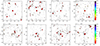 |
Fig. A.1. As in Fig. 3 but showing in color only galaxies with SFRs lower than ∼ 5 M⊙ yr−1. |
| In the text | |
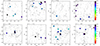 |
Fig. A.2. As in Fig. 3 but showing in color only galaxies with SFRs larger than ∼ 80 M⊙ yr−1. |
| In the text | |
|
Fig. A.3. The star formation histories of galaxies in the bottom 25th (cyan) and highest 75th (magenta) percentiles of the distribution of o3. Ticker lines show the median star formation histories. The numbers of galaxies in each sub-sample at each snapshot is given in the top left corner. A maximum of 50 individual star formation histories in each subsample is shown to avoid overcrowding the panels. |
| In the text | |
|
Fig. A.4. As in Fig. 9, but cyan and magenta histograms in the top and middle panel corresponds to galaxies in the extreme of the n3 distribution. The bottom panel shows the correlation between the halo mass in which descendants of quiescent high-z galaxies reside at z = 0 and n3 at the time of observation. |
| In the text | |
Current usage metrics show cumulative count of Article Views (full-text article views including HTML views, PDF and ePub downloads, according to the available data) and Abstracts Views on Vision4Press platform.
Data correspond to usage on the plateform after 2015. The current usage metrics is available 48-96 hours after online publication and is updated daily on week days.
Initial download of the metrics may take a while.