| Issue |
A&A
Volume 700, August 2025
|
|
|---|---|---|
| Article Number | A46 | |
| Number of page(s) | 26 | |
| Section | Extragalactic astronomy | |
| DOI | https://doi.org/10.1051/0004-6361/202553708 | |
| Published online | 07 August 2025 | |
The SRG/eROSITA all-sky survey
Subaru/HSC-SSP weak-lensing mass measurements for eRASS1 galaxy clusters
1
Physics Program, Graduate School of Advanced Science and Engineering, Hiroshima University, 1-3-1 Kagamiyama, Higashi-Hiroshima, Hiroshima 739-8526, Japan
2
Hiroshima Astrophysical Science Center, Hiroshima University, 1-3-1 Kagamiyama, Higashi-Hiroshima, Hiroshima 739-8526, Japan
3
Core Research for Energetic Universe, Hiroshima University, 1-3-1, Kagamiyama, Higashi-Hiroshima, Hiroshima 739-8526, Japan
4
Argelander-Institut für Astronomie (AIfA), Universität Bonn, Auf dem Hügel 71, 53121 Bonn, Germany
5
Universität Innsbruck, Institut für Astro- und Teilchenphysik, Technikerstr. 25/8, 6020 Innsbruck, Austria
6
Department of Physics, National Cheng Kung University, No.1, University Road, Tainan City 70101, Taiwan
7
Center for Frontier Science, Chiba University, 1-33 Yayoi-cho, Inage-ku Chiba 263-8522, Japan
8
Department of Physics, Graduate School of Science, Chiba University, 1-33 Yayoi-Cho, Inage-Ku, Chiba 263-8522, Japan
9
Institute of Astronomy and Astrophysics, Academia Sinica, P.O. Box 23-141 Taipei 10617, Taiwan
10
Max Planck Institute for Extraterrestrial Physics, Giessenbachstrasse 1, 85748 Garching, Germany
11
IRAP, Université de Toulouse, CNRS, UPS, CNES, Toulouse, France
12
INAF, Osservatorio di Astrofisica e Scienza dello Spazio, Via Piero Gobetti 93/3, I-40129 Bologna, Italy
13
Institute for Frontiers in Astronomy and Astrophysics, Beijing Normal University, Beijing 102206, China
⋆ Corresponding author: This email address is being protected from spambots. You need JavaScript enabled to view it.
Received:
9
January
2025
Accepted:
12
June
2025
Abstract
We performed individual weak-lensing (WL) mass measurements for 78 eROSITA’s first All-Sky Survey (eRASS1) clusters in the footprint of Hyper Suprime-Cam Subaru Strategic Program (HSC-SSP) S19A. We did not adopt priors on the eRASS1 X-ray quantities or assumption of the mass and concentration relation. In the sample, we found three clusters are misassociated with optical counterparts and 12 clusters are poorly fitted with an NFW profile. The average mass for the 12 poor-fit clusters changes from ∼ 1014 h70−1 M⊙ to ∼ 2 × 10¹³ h70−1 M⊙ when lensing contamination from surrounding mass structures is taken into account. The scaling relations between the true mass and cluster richness and X-ray count-rate agree well with the results of the eRASS1 western Galactic hemisphere region based on count-rate-inferred masses, which were calibrated with the HSC-SSP, DES, and KiDS surveys. We developed a Bayesian framework for inferring the mass-concentration relation of the cluster sample, explicitly incorporating the effects of weak-lensing mass calibration in the mass-concentration parameter space. The redshift-dependent mass and concentration relation is in excellent agreement with predictions of dark-matter-only numerical simulations and previous studies using X-ray-selected clusters. Based on the two-dimensional (2D) WL analysis, the offsets between the WL-determined centers and the X-ray centroids for 36 eRASS1 clusters with high WL S/N can be described by two Gaussian components. We find that the miscentering effect with X-ray centroids is smaller than that involving peaks in the galaxy maps. Stacked mass maps support a small miscentering effect, even for clusters with a low WL S/N. The projected halo ellipticity is ⟨ε⟩ = 0.45 at M200 ∼ 4 × 10¹⁴ h70−1 M⊙, which is in agreement with the results of numerical simulations and previous studies of clusters characterized by masses greater than twice the mass treated here.
Key words: gravitational lensing: weak / galaxies: clusters: general / galaxies: clusters: intracluster medium / X-rays: galaxies: clusters
© The Authors 2025
 Open Access article, published by EDP Sciences, under the terms of the Creative Commons Attribution License (https://creativecommons.org/licenses/by/4.0), which permits unrestricted use, distribution, and reproduction in any medium, provided the original work is properly cited.
This article is published in open access under the Subscribe to Open model. This email address is being protected from spambots. You need JavaScript enabled to view it. to support open access publication.
1. Introduction
The evolution of the cluster mass function provides powerful constraints on cosmological parameters, in particular, the energy density of the total matter, normalization of density fluctuation, and dark energy (e.g., Chiu et al. 2023; Ghirardini et al. 2024; Artis et al. 2024, 2025). Since the X-ray emissivity of thermal bremsstrahlung is proportional to the square of the electron number density, X-ray observations, which are less sensitive to projection effects, serve as a powerful tool for searching for galaxy clusters. The eROSITA (extended ROentgen Survey with an Imaging Telescope Array; Merloni et al. 2012; Predehl et al. 2021) instrument on board the Spectrum Roentgen Gamma (SRG) mission (Sunyaev et al. 2021) is a unique tool that enables the discovery of galaxy clusters on an order of 105. Indeed, the eROSITA Final Equatorial Depth Survey (eFEDS) in a footprint with an area of ∼140 deg2, significantly overlapping the Subaru/HSC-SSP footprint (Aihara et al. 2018, 2022), found 542 cluster candidates (Liu et al. 2022) and confirmed an optical counterpart of 477 clusters and groups (Klein et al. 2022). Recently, the Western Galactic Hemisphere of the eROSITA’s first All-Sky Survey (the eRASS1; Bulbul et al. 2024; Kluge et al. 2024) discovered 12 247 optically confirmed galaxy groups and clusters detected in the 0.2–2.3 keV over 13 116 deg2 and constructed a sample for cosmology (Bulbul et al. 2024), with a high purity level of ∼95%, comprising 5259 optically confirmed clusters over an area of 12 791 deg2.
Accurate mass measurements of galaxy clusters are vitally important for cluster cosmology. Thanks to deep and wide optical surveys of ground-based telescopes of Subaru/HSC-SSP, DES, and KiDS (Chiu et al. 2022, 2025; Grandis et al. 2024; Kleinebreil et al. 2025), the weak gravitational lensing effect can measure mass structures without assumptions of dynamical states. The weak-lensing (WL) mass measurements for eROSITA utilize a hierarchical Bayesian approach to simultaneously fit the tangential shear profiles, accounting for the mass and count-rate relation in individual clusters. (Chiu et al. 2022, 2025; Grandis et al. 2024). The resulting WL mass is, therefore, a kind of count-rate-related mass. The adopted mass model assumes the mass and concentration relation for a Navarro-Frenk-White (NFW) model (Navarro et al. 1996, 1997) statistically treats miscentering effects by convolving a probability function, using the relationship between the true and WL masses based on numerical simulations.
In contrast, the individual cluster WL analysis allows for the concurrent determination of the two parameters of mass and concentration; however, it does necessitate a large number of background galaxies (e.g., Okabe & Smith 2016; Umetsu et al. 2020). Furthermore, two-dimensional WL analyses (Oguri et al. 2010) enable us to measure central positions for the assumed mass models to assess the miscentering effect utilized in the statistical WL mass measurement. The lensing information also independently provides us with the purity of the detected clusters. Therefore, individual cluster lensing measurement is complementary to statistical cluster-lensing analysis.
Thanks to the deep imaging of the Subaru/HSC-SSP, we were able to perform cluster mass measurements for the eRASS1 clusters to understand and control WL systematics. The paper is organized as follows. We describe the WL mass measurement techniques in Sect. 2, followed by our results in Sect. 3, a discussion in Sect. 4, and conclusions in Sect. 5, respectively. Throughout the paper, we use Ωm, 0 = 0.3, ΩΛ, 0 = 0.7, and H0 = 70 h70 km s−1 Mpc−1 = 100 h km s−1 Mpc−1, with h70 = 1 and h = 0.7.
2. Weak-lensing analysis
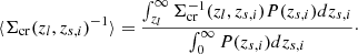
We selected 78 clusters (Table E.1 and Fig. 1) for weak-lensing mass measurements from the 103 eRASS1 clusters in the HSC-SSP S19A footprint, according to the following criteria; the area fraction within  centering the eRASS1 primary clusters (Ghirardini et al. 2024), where an HSC-Y3 shape catalog (see details in Li et al. 2022) is available, is greater than 70% and the innermost radius is less than
  . For instance, 23 clusters were removed because they are located around the edge of the HSC-Y3 footprint, so the galaxies in the shape catalog are not distributed in all azimuthal directions but only on one side or a small patch region. The central areas of the other two clusters are unavailable due to star masks, rendering them inaccessible.
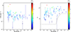 |
Fig. 1. Left: Count-rate (CR) versus redshift (z). Right: Richness (λ) versus redshift (z). The dotted line is the threshold described by a function connecting two constants with a linear function. Colors in all the panels denote the S/N of the reduced tangential shear profile. The circles, diamonds, squares, and up-triangles denote the clusters with 1D WL analysis only, 1D and 2D WL analysis, non-WL analysis, and misassociation, respectively. |
2.1. Background selection
The HSC-Y3 shape catalog uses a method based on point spread function (PSF) correction known as re-Gaussianization (Hirata & Seljak 2003), which is implemented in the HSC pipeline (see details in Mandelbaum et al. 2018a; Li et al. 2022). In weak-lensing mass measurements, we utilize galaxies from the HSC galaxy catalog that meet the full-color and full-depth criteria, ensuring accurate shape measurement and reliable photometric redshift estimation. We selected background galaxies behind each cluster based on the condition (Medezinski et al. 2018):
 (1)
(1)
where P(z) is the probability of the photometric redshift from the machine learning method (MLZ; Carrasco Kind & Brunner 2014) calibrated with spectroscopic data (Tanaka et al. 2018; Nishizawa et al. 2020) and zl is a cluster redshift. After the background selection, the number density of background galaxies has a strong redshift dependence, varying from ∼2 to ∼12 [arcmin−2], with an average of 7.0 ± 2.5 [arcmin−2] (Figs. 2 and B.1).
2.2. Mass estimation
The reduced tangential shear ΔΣ+ was computed by the azimuthal averaging the measured tangential ellipticity, e+, for i-th galaxy in a given k-th annulus,
 (2)
(2)
where e+ is the tangential ellipticity (e+ = −(e1cos2φ + e2sin2φ), wi is the weighting function, ⟨Σcr(zl, zs, i)−1⟩ is the inverse of the mean critical surface mass density, ℛ is the shear responsivity, and K is the calibration factor. The weighting function is given by
 (3)
(3)
where erms and σe are the root mean square of intrinsic ellipticity and the measurement error per component (α = 1 or 2), respectively. The inverse of the mean critical surface mass density is computed by the probability function, P(z), following
 (4)
(4)
Here, zl and zs are the cluster and source redshift, respectively. The critical surface mass density is Σcr = c2Ds/4πGDlDls, where Ds and Dls are the angular diameter distances from the observer to the sources and from the lens to the sources, respectively. The shear responsivity is expressed as (see Mandelbaum et al. 2005; Reyes et al. 2012):
 (5)
(5)
The measured values are corrected by the shear calibration factor (m, c) for individual objects (Li et al. 2022), where m is a multiplicative calibration bias and c an additive residual shear offset in the relation between the input and output shear component, γoutput, α = (1 + mα)γinput, α + cα, as defined by STEP (Shear TEsting Programme) simulations (Heymans et al. 2006; Massey et al. 2007). The calibration factor, K, is computed by
 (6)
(6)
where mi for individual galaxies are estimated based on GREAT3-like simulations (Mandelbaum et al. 2018b, 2014, 2015) as a part of the GREAT (GRavitational lEnsing Accuracy Testing) project. We then subtract
 (7)
(7)
from ⟨ΔΣ+⟩(ri) (Eq. (2)). The additional offset term is negligible 𝒪(< 10−4) compared to 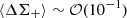 . The effective radius utilized to characterize the tangential shear in each annulus is shifted from the intermediate radius since parts of the galaxy distributions are partially missing due to the presence of a star mask. We thus adopted the weighted harmonic mean as the radius positions,
 (8)
(8)
which aptly explains a power-law tangential shear profile (Okabe & Smith 2016).
We employed an NFW profile (Navarro et al. 1996) for model fitting. The NFW mass density profile is described as
 (9)
(9)
where ρs is the central density parameter and rs is the scale radius. We used two parameters of the spherical mass, MΔ, and the halo concentration, cΔ, instead of ρs and rs. The spherical mass and the halo concentration are defined by
 (10)
(10)
respectively. Here, ρcr(z) is the critical mass density at the cluster redshift and Δ is the overdensity. The reduced shear model, fmodel, is described using the differential surface mass density  and the local surface mass density Σ as follows,
 (11)
(11)
where  . The log-likelihood is expressed as
 (12)
(12)
where the covariance matrix, C, is composed of the uncorrelated large-scale structure (LSS), CLSS, along the line of sight (Schneider et al. 1998), the shape noise, Cg, and the error of photometric redshift, Cs. We also adopted the maximum likelihood estimation (MLE).
When we compute the reduced tangential shear from a small number of background galaxies, any internal substructures or surrounding clusters might accidentally affect mass measurements. In such cases, we can adopt the adaptive choice of binning scheme (e.g., Okabe & Smith 2016) via the following procedure. We first fit the NFW model to 270 radial combinations of the measured ΔΣ+ profile; the innermost radii ![Mathematical equation: $ r_{\mathrm{in}}=[0.1{-}0.2]\,{{h_{70}^{-1}\,\mathrm{Mpc}}} $](/articles/aa/full_html/2025/08/aa53708-25/aa53708-25-eq21.gif) stepped by 0.05
stepped by 0.05 , the outermost radii
 ![Mathematical equation: $ r_{\mathrm{out}}=[2{-}3.6] \,{{h_{70}^{-1}\,\mathrm{Mpc}}} $](/articles/aa/full_html/2025/08/aa53708-25/aa53708-25-eq23.gif) stepped by 0.2
stepped by 0.2  , and the number of bins Nbin = [4 − 8] stepped by 1. We then estimated the mean masses of the suite of MΔ within the overdensities of Δ = 2500, 100, 500, 200, and vir and chose a radial bin set closest to the mean values. If the innermost galaxy is farther away than rin, the first radius of rin is taken as its position without changing the annulus width. To minimize lensing contamination from the nearest clusters in the reduced tangential shear profile, we computed the distance between the target cluster and the nearest one from the eRASS1 cluster catalog. If the distance between two clusters is smaller than the maximum radius rout, the maximum radius is set to half this distance. It is important to note that we refrain from utilizing any external catalogs to identify neighboring clusters when aiming to achieve mass measurements in a self-consistent way.
2.3. Weak-lensing mass reconstruction
After background selection, we pixelize the shear distortion data in a regular grid of pixels using a Gaussian kernel, G ∝ exp[−θ2/(2σg2)] with  . In the mass reconstruction, we assumed the WL limit as
  where α = 1, 2. The dimensional shear field at angular position θ is obtained by
 (13)
(13)
where  and
and  are computed with a lensing weight added by the Gaussian kernel, that is, wi is replaced by wiG(θi − θ) in Eqs. (5) and (6). Since the above Gaussian smoothing is the convolution integral, we performed it in the Fourier space at the same time as the Kaiser & Squires (KS) inversion method (Kaiser & Squires 1993) to invert the pixelized shear field to the mass map. If there were blank areas due to the bright star mask in a map-making field, we filled in dummy data in the region and mask it after the mass reconstruction. The spatial positions of the dummy are generated from a random uniform distribution. The shape and photo-z data of the dummy are taken randomly from the real data and the ellipticities were then randomly rotated. We estimated the mass reconstruction errors by the bootstrapping method. We fixed the positions of background galaxies and randomly rotated an ellipticity component taken from other galaxies. This was repeated for 500 realizations and the error is estimated as the standard error of the mock mass maps. The S/N for the mass map is obtained by dividing the reconstructed mass maps by the noise maps. As for the stacked mass maps (Sects. 3.7 and 3.9), we first combined the background shape catalogs, converting the celestial positions and ellipticities to those measured at the reference coordinates (Okabe et al. 2013, 2019), and then we ran the KS inversion method. We adopted FWHM
  and 1′ for the individual and stacked map making, respectively.
2.4. 2D WL analysis
The mass modeling using the 2D shear pattern enables us to parameterize both the central positions and the mass parameters of clusters (Oguri et al. 2010). The miscentering effect is one of the important parameters for the simultaneous analysis of ensemble samples of clusters (Chiu et al. 2022, 2025; Grandis et al. 2024). For this purpose, we computed the shear grids every 1.5 arcmin in a square box of half-size 3  Mpc, centering the eRASS1 positions. The ensemble averages of the ellipticity components and positions are calculated similarly to Eqs. (2) and (8), respectively. The log-likelihood is expressed as
 (14)
(14)
where the indices α and β are the two components of shear distortion. We considered shape noise only in the covariance matrix to reduce the computation time. We employed three distinct mass models: the spherical NFW model, an elliptical NFW mass model, and a multi-component model of the spherical NFW model (Okabe et al. 2011). The spherical NFW model is the same as that used in the 1D WL analysis.
The elliptical NFW model (see also Oguri 2021, for fast computation) takes into account the ellipticity of the mass distribution on the sky plane (Oguri et al. 2010; Golse & Kneib 2002). The 2D halo ellipticity, ε, is defined by 1 − b/a, where a and b are the major and minor axes of the mass distribution on the sky plane, respectively. The distances from the centers to the iso-contours are calculated by
 (15)
(15)
Here, ϕe is an orientation angle of the major axis measured from the north to the east.
If there are multiple clusters in the data field, the center of a single NFW model might be affected. In this case, we consider the multi-component spherical NFW model. If the mass map has a peak of more than 4σ, which is the FWHM away from the eRASS1 centroids, we would add mass components other than the target clusters at its peak-finding position to investigate how much the WL-determined central positions are changed. We assumed the mass-concentration relation (Diemer & Kravtsov 2015) for clusters that are not being specifically targeted.
We used the Markov chain Monte Carlo (MCMC) method and treated the logarithmic quantities for M200 and c200 as parameters because they are positive. We used flat priors for all the parameters; ![Mathematical equation: $ |\mathrm{RA}-\mathrm{RA}_{\mathrm{eRASS1}}| < 3\,[h_{70}^{-1}\,\mathrm{Mpc}]/D_l $](/articles/aa/full_html/2025/08/aa53708-25/aa53708-25-eq34.gif) ,
, ![Mathematical equation: $ |\mathrm{Dec}-\mathrm{Dec}_{\mathrm{eRASS1}}| < 3\,[h_{70}^{-1}\,\mathrm{Mpc}]/D_l $](/articles/aa/full_html/2025/08/aa53708-25/aa53708-25-eq35.gif) ,
,  , and ln1 < lnc200 < ln30. Regarding halo ellipticity and orientation angle, we used −1 < e < 1 and 0 < ϕe < 2π to avoid an artificial boundary around e = 0 and ϕe = 0, π and then used absolute values for e and superimposed a double-peak posterior distribution for ϕe in the estimation. All parameters were estimated using a central bi-weight estimation from marginalized posterior distributions to down-weight outliers in skewed distributions.
3. Results
3.1. Cluster sample
The X-ray count-rate (CR) was estimated in the soft-band (0.2–2.3 keV) with correction of Galactic absorption (Bulbul et al. 2024). The CR of the eRASS1-HSC clusters has a weak dependence on redshift (the left panel of Fig. 1), as expected by the CR selection function. The average and median CRs are  and 0.56, respectively. When we remove the first two with the highest CR, the average drops to 0.66. The richness is measured by an adapted version of the redMaPPer (Rykoff et al. 2014) algorithm (Kluge et al. 2024). The lower boundary of the cluster richness λ (the right panel of Fig. 1) at high redshift (z ≳ 0.6) is higher than at low redshift (z ≲ 0.4). This indicates that less massive clusters are harder to detect at higher redshifts (Clerc et al. 2024). We effectively adopted the detection threshold λ = 3 at z < 0.45 and 30 at z > 0.6 and a linear function between the two redshifts to consider the selection function in the mass-richness scaling relation.
We matched the eRASS1 clusters in the HSC footprint to existing cluster catalogs (Abell 1958; Zwicky et al. 1961; Wen et al. 2009; Oguri et al. 2018; Koester et al. 2007; Gal et al. 2009; Goto et al. 2002; Von Der Linden et al. 2007; Dietrich et al. 2007; Popesso et al. 2004; Mehrtens et al. 2012; Hilton et al. 2021), as summarized in Table E.1. The tolerance of cross-matching is 3 arcmin for the spatial separation and |z − zeRASS1|< 0.05. If there are multiple associations of optically selected clusters, the priority is given to putting WHL clusters (Wen et al. 2009) or HSC CAMIRA clusters (Oguri et al. 2018). From the well-known cluster catalogs, we found 12 Abell clusters (Abell 1958), 2 Zwicky clusters (Zwicky et al. 1961), 2 X-ray clusters, and 5 SZ clusters (Hilton et al. 2021) in the sample. As one of the samples, Fig. 3 shows the mass map overlaid with X-ray contours from eRASS1 and XMM-Newton data for J141507.1-002905 and J141457.8-00205 field, which is known as MCXC J1415.2-0030 (Piffaretti et al. 2011).
We carried out a visual inspection of the purity using HSC images, publicly available spectroscopic redshifts, and the spatial distribution of red-sequence galaxies. It would be difficult to do this with each of the over 5000 clusters of the primary sample (Ghirardini et al. 2024), but it is practically possible in the current HSC sample. The HSC images were extracted with 4′×4′ centered on the centroid of the eRASS1 cluster. We overlaid spectroscopic redshifts from the publicly available catalogs (Baldry et al. 2018; Aguado et al. 2019; Lilly et al. 2009; Colless et al. 2003) and monitored the difference with the eRASS1 redshifts. We constructed Gaussian smoothing maps (FWHM  ) of the number distribution of red sequence galaxies selected in the color-magnitude plane following Nishizawa et al. (2018), Okabe et al. (2019). The apparent z-band magnitudes of the red-sequence galaxies are brighter than the observer-frame magnitude with the constant z-band absolute magnitude of Mz = −18 ABmag and the limiting apparent magnitude mz = 25.5. We employed K-correction to convert between apparent and absolute magnitudes, considering passive evolution. Henceforth, clusters possessing and lacking optical counterparts are referred to as association clusters and misassociation clusters, respectively.
Based on the spectroscopic redshifts, we found three misassociation clusters: J114647.4-012428, J123108.4+003653, and J124503.8-002823 (Fig. 4). Although we examined the galaxy overdensities sliced by each redshift, we could not find any significant excess, as shown by the white contours. The X-ray centroid of J114647.4-012428 (left panel, z = 0.33) is associated with two ellipticals at z ∼ 0.14. WHL J1146416-012324, with a close redshift of z = 0.3318, is 1.9 arcmin away from J114647.4-012428. The X-ray emission of J123108.4+003653 (middle panel, z = 0.47) is associated with two galaxies identified as MCXC J1231.0+0037 at z ∼ 0.023. WHL J123122.9+003718 at z = 0.4354 is 3.6 arcmin away from J123108.4+003653 outside the HSC image (Fig. 4). The X-ray emission from J124503.8-002823 (right panel, z = 0.23) apparently comes from a nearby spiral galaxy, NGC 4666. WHL J124454.5-002640 at z = 0.231 is 3.3 arcmin away from J124503.8-002823 and its galaxy concentration is found.
We note that the fraction of the misassociation clusters in the HSC-SSP field, 3/78 ∼ 4%, is consistent with the ∼95% purity of the primary clusters (Clerc et al. 2024; Kluge et al. 2024).
3.2. Weak-lensing mass measurements
We first calculated the signal-to-noise ratio (S/N) of the reduced tangential shear profile by  , where the indexes i and j denote the i-th and j-th radial bins, respectively. The average and median S/N are 4.5 and 4.3, respectively. In the CR and z plane (left panel in 1), the S/N is higher for clusters with higher CR around z ∼ 0.1 − 0.4, because the clusters have good lensing efficiency and a large number of background galaxies. The clearer feature is found in the richness and z plane (right panel of Fig. 1). The S/N tends to be higher for the clusters in the upper left corner of the figure.
The individual WL masses for the 72 association clusters are shown in Table E.1. Among all the 78 clusters, we cannot measure WL masses of the three association clusters and the three misassociation clusters. The number of non-measurable clusters in the 75 association clusters is consistent with the expectation computed by mock catalogs using a realistic number density of background galaxies (see Appendix B and Fig. B.1). The measurement uncertainties for nine association clusters are too large. Thus, only an upper limit on the WL masses can be constrained. We refer to the 12 association clusters above, whose WL masses at Δ = 500 are difficult or impossible to measure, as poor-fit clusters (Table E.1). The WL masses as a function of the redshift are shown in Fig. 2. With increasing redshifts, the WL masses tend to be larger and at lower redshifts (z ≲ 0.2), they span a broad range of values. The modeled distribution of the WL masses in the parent population obtained via a scaling relation analysis (see the details in Sect. 3.4) follows this trend.
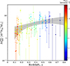 |
Fig. 2. Weak-lensing masses ( |


3.3. Stacked tangential shear profiles
We computed the stacked tangential shear profiles for the 3 misassociation clusters, the 12 poor-fit clusters, and 63 other association clusters (Fig. 5). The number of bins was set to six because of the small number of background galaxies for the three misassociation clusters. To visualize the null signal for the misassociation clusters, we used r times the tangential shear, ⟨Σ+⟩, or the 45-degree rotated component, ⟨Σ×⟩, for the y axis. The tangential shear component for the misassociation clusters is comparable to the 45-degree rotated component and consistent with the null, supporting the visual inspection result (Sect. 3.1). In contrast, the lensing signals for the poor-fit and remaining 63 clusters are significantly detected with S/N = 7.0 and 34.0, respectively.
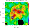 |
Fig. 3. Mass map for the J141507.1-002905 and J141457.8-00205 field (30′×30′). The black contours represent the reconstructed WL mass map spaced in units of 1σ bootstrapping error. The diameter of the black circle in the lower left corner represents the Gaussian smoothing FWHM = 400 kpc in the mass reconstruction. Blacked-out areas are the masked regions of bright stars. The blue + and × are positions of J141507.1-002905 and J141457.8-00205, respectively. The system is MCXC J1415.2-0030 (Piffaretti et al. 2011). The blue and cyan contours are the eRASS1 and XMM-Newton X-ray contours (Miyaoka et al. 2018), respectively. An X-ray bright point source in the western component is removed in the XMM-Newton contours. It was properly identified when the eRASS1 cluster catalog was constructed. At the same time, diffuse X-ray emission in the XMM-Newton image appeared even after removing the X-ray point source thanks to a higher angular resolution. The system is composed of three components with S/N ∼ 6.7σ for J141457.8-00205, ∼4.7σ for J141507.1-002905, and ∼5.3σ for the western component. |
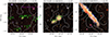 |
Fig. 4. HSC images for misassociation clusters. Overlaid with white contours representing red galaxy distribution, stepped by two galaxies per each pixel above two galaxies. |
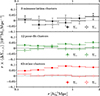 |
Fig. 5. Stacked profiles for the three misassociation clusters (top), the 12 poor-fit clusters (middle), and the 63 other clusters (bottom). The y-axis represents r × ⟨Σ+⟩ (filled colors) or r × ⟨Σ×⟩ (open colors). The + components for the 63 other clusters and the 12 poor-fit clusters are higher than the × components, while both the + and × components for the 3 misassociation clusters are consistent with the null. |
We divided the remaining 63 clusters into three samples by redshift: 0.4 < z, 0.2 < z ≤ 0.4, and 0.1 < z ≤ 0.2 (Fig. 6). The S/Ns are 12.9, 19.1, and 23.6 in the order of higher redshift, respectively. The tangential shear profile distinctly exhibits curvature. The tangential shear profile for the poor-fit clusters shows a depletion in an intermediate radius of 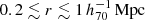 (Sect. 3.8).
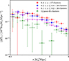 |
Fig. 6. Stacked tangential profiles for 3 subsamples divided by redshift ranges of 0.4 < z (red diamonds), 0.2 < z ≤ 0.4 (blue squares), and 0.1 < z ≤ 0.2 (magenta upward triangles), and the 12 poor-fit clusters (green downward triangles). The filled and open symbols denote positive and negative values, respectively. |
3.4. Mass-richness-CR relation
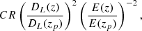
We computed the scaling relations between the extinction corrected CR and the WL masses and between the richness of the cluster and the WL masses of the 72 individual clusters, excluding 3 clusters with no mass measurements (Fig. 7). The CR is multiplied by the square of the luminosity distance, DL(z), and the inverse square of  to correct the redshift evolution (Chiu et al. 2022; Ghirardini et al. 2024), specified as
 (16)
(16)
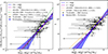 |
Fig. 7. Scaling relations between the count-rate (left) the richness (right) and the WL ( |

where zp is a pivot redshift 0.21 as a lensing weight average from stacked lensing analysis. For the logarithmic quantity, we express the correction term as

Both the corrected CR and the richness are highly correlated with the WL masses (Fig. 7). To quantify the relationships between mass, CR, and richness, we adopt the trivariate scaling relations, including the relation between the WL masses ( ), and the true masses (
 ), the so-called WL mass calibration. In general, the WL mass calibration consists of two effects: astrophysical (intrinsic) properties and observational conditions. The former is mainly due to the orientation of elliptical halos, the presence of subhalos, and their surroundings (Meneghetti et al. 2010; Becker & Kravtsov 2011; Giocoli et al. 2012; Euclid Collaboration: Giocoli et al. 2024). The adaptive choice of radial bins could reduce these effects as much as possible (Okabe et al. 2016). The latter is associated with the number of background galaxies. When combining the gravitational lensing effect with the intrinsic ellipticity of a small number of background galaxies, the resulting S/N exhibits random variation and the measurable masses are restricted to those exhibiting a notably high bias. Since the number density of our background galaxies strongly depends on cluster redshifts (Figs. 2 and B.1), we cannot rule out such a selection bias in successful individual WL mass measurements. To quantify selection bias, we performed mock simulations empirically representing observational conditions using a spherical NFW model (see details in Sect. B). We made 9000 mock shape catalogs and repeated our analysis without lensing effect from large-scale structure. The measurable fraction decreases as the cluster redshift increases and the mass decreases, so the measured WL mass has a higher positive bias as the cluster redshift increases and the mass decreases. With a selection function, the WL mass calibration is well described by a redshift-dependent linear equation of the logarithmic quantities (Eq. (17)) and is used as a prior in a regression analysis. We note that our WL mass calibration based on two parameters is different from the one-parameter case (Chiu et al. 2022; Grandis et al. 2024).
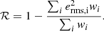
We used a hierarchical Bayesian regression method (Akino et al. 2022; Sereno 2016) to infer the true mass distribution of the parent population, taking into account the selection effect. We assume that the logarithm of the true mass follows a Gaussian distribution 𝒩(μ(z),σ(z)) of which mean (μ) and standard error (σ) are a polynomial function of F(z) = ln((1 + z)/(1 + zp)). We used the second-order and first-order polynomial functions for the mean and standard error, respectively. As shown in Akino et al. (2022), the model realizes well the input of multivariate scaling relations in samples of ∼ 𝒪(100) clusters, regardless of the shape of the parent population, such as the Gaussian distribution and the cluster mass function. Its advantage is that it is independent of the cluster mass function or cosmological parameters. We adopted the lower limits for the corrected CR and the richness as 0.01 and the line in Fig. 1, respectively. In the regression analysis, we use the following equations (see also Ghirardini et al. 2024; Grandis et al. 2024):
 (17)
(17)
 (18)
(18)
 (19)
(19)
where Mp, CRp, and λp are a pivot mass  , a pivot count-rate 1 cnt s−1, and a pivot richness 40, respectively. The normalization, the mass-dependent slope, the redshift-dependent slope in the normalization, and the redshift-dependent slope in the mass-related slope are expressed by α, β, γ, and δ, respectively. The deviation from the self-similar model is quantified by γ and δ (e.g., Bulbul et al. 2019; Chiu et al. 2022; Ghirardini et al. 2024).
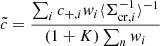
The intrinsic covariance (Okabe et al. 2010) is described by
 (20)
(20)
where σ and r are the intrinsic scatter of the left-hand-side quantities of Eqs. (17)–(19) and the intrinsic coefficient between two variables, respectively. We assume that the intrinsic covariance is independent of the redshift. We use the WL mass bias parameters as priors (Appendix. B), taking into account their error covariance matrix.
We first performed a regression analysis for three cases:(1) rCR, WL = rλ, WL = 0, (2) δ = 0, and (3) all the free parameters. The resulting parameters are shown in Table 1. The intrinsic coefficients, rCR, WL and rλ, WL, are not well constrained in the three cases and are consistent with 0. In contrast to Ghirardini et al. (2024), the errors of redshift-dependent slopes δ and γ are large because of our small sample size. We then fix rCR, WL = rλ, WL = 0 and δ = 0, which is referred to as (4).
Best-fit parameters for the mass-richness-CR relation.
We assessed the models by employing the Akaike’s information criterion (AIC) and Bayesian information criterion (BIC) to determine which model aligns most closely with reality. The deviations of the AIC and BIC of (1)–(3) from (4) give larger values with +5 ∼ +22. When we additionally fixed γ = 0, ΔAIC and ΔBIC worsened even by +9 and +3, respectively. Therefore, we chose to focus on the result of (4), as shown in Fig. 7. The blue and magenta solid lines represent the best-fit scaling relations concerning the WL and true masses (Fig. 7), respectively.
The mass-dependent slope for CR and mass scaling relation is consistent with 1. The mass-dependent slope for the richness and mass scaling relation confirms that the number of cluster galaxy members is proportional to the cluster mass. Although the redshift dependencies of the normalization are not well constrained, the normalization for the CR and the richness are likely to increase and decrease as the redshift increases, respectively. The intrinsic scatter for the two scaling relations is ∼30%. We find that the intrinsic coefficient between the CR and richness is consistent with zero.
Stacked lensing results are indicated by blue diamonds, regardless of the success of individual mass measurements. The three sub-samples are divided by the richness with λ ≤ 40, 40 < λ < 70, and 70 ≤ λ. Since the number of background galaxies and the lensing efficiency for individual clusters are different from each other, we computed the average values with a lensing weight of  , where i and j are the indexes for the clusters and their background galaxies, respectively. The stacked quantities coincide with the baseline with the WL mass.
The Bayesian analysis also gives us the parent population of the true mass  , which leads to the
  distribution of the parent population. As shown in Fig. 2, the
  distribution represents well the measured
  of the observed sample. When we change the order of the polynomial function to either 1 or 3, the result does not change. When we use the 2nd order polynomial function for the standard error, both the AIC and BIC get worse by +1 and +4, respectively. The current model is thus sufficient to describe the sample.
We artificially change the intrinsic scatter of the WL mass calibration to σWL = 0.214 calibrated with synthetic weak-lensing observations (Umetsu et al. 2020) of 639 cluster halos in a dark-matter-only realization of BAHAMAS simulations (McCarthy et al. 2017) at a single redshift z = 0.25. The analysis was repeated with just σWL adjusted to this redshift-independent value, while keeping the other parameters the same. We find that γ and σint for the two scaling relations change by ∼ + 20% and ∼ − 10%, respectively.
Since our WL mass measurements do not use informative priors, it is easy to find out the outliers, such as the poor-fit clusters. When we remove the 12 poor-fit clusters, we find that the baseline parameters do not change significantly and the intrinsic scatter of the CR and the richness become ∼8% lower, though they are consistent with each other within 1σ.
3.5. Mass-concentration relation
Numerical simulations (e.g., Bullock et al. 2001; Bhattacharya et al. 2013; Child et al. 2018; Diemer & Joyce 2019; Ishiyama et al. 2021) predict that the halo concentration for the NFW mass model increases with decreasing halo mass and redshift. Such an anti-correlation between mass and concentration can be explained by hierarchical structure formation. The progenitors of less massive halos form first and their characteristic central mass density is reflected by a critical density at higher redshifts. More massive halos form later, with lower mass densities than the less massive halos, and grow by mass accretion and mergers of smaller objects. Some simulations show that the concentration turns upward for the most massive halos (e.g., Prada et al. 2012; Klypin et al. 2016). This upturn feature is still controversial (e.g., Prada et al. 2012; Diemer & Kravtsov 2015; Klypin et al. 2016; Child et al. 2018). The concentration also depends on the dynamical state, that is, relaxed halos have a higher concentration than unrelaxed halos (e.g., Dutton & Macciò 2014; Klypin et al. 2016; Ishiyama et al. 2021).
The mass and concentration give us a unique opportunity to test how structures form at cluster scales. Thanks to X-ray emissivity, X-ray centroid determination does not suffer from projection effects as in the case of optically selected clusters (e.g., Okabe & Smith 2016; Umetsu et al. 2016, 2020; Okabe et al. 2019).
The mass and concentration of the 72 association clusters for which WL masses were measured are shown in Fig. 8. Since these errors are correlated, the 1σ banana-shaped regions are shown in transparent gray. To model the mass and concentration relation, we adopted the following relation
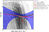 |
Fig. 8. WL mass and concentration relation at Δ = 200. The transparent gray banana regions represent the 1σ constraint on mass and halo concentration for the 72 association clusters. The orange and red shaded regions represent the 1σ constraints by stacked lensing analysis for the 53 clusters with single galaxy peaks and the 22 clusters with multiple galaxy peaks, respectively. The best-fit line and its 1σ uncertainty are shown as the blue solid line and region, respectively. The magenta line is the best-fit for the true mass and the true concentration. The brown, pink, red, and green lines are the results of numerical simulations of Bhattacharya et al. (2013), Child et al. (2018), Diemer & Joyce (2019), and Ishiyama et al. (2021), respectively. |
 (21)
(21)
with cp = 4 and an intrinsic scatter of σc. The reference redshift is set to be the lensing weight average of zp = 0.21 for the 72 association clusters. We considered the correlation between the errors in mass and concentration, as well as the WL mass calibration, during the fitting process (see Appendix A). Since the mass and concentration parameters were measured simultaneously, we evaluated the WL mass calibration as a mass and concentration plane with the intrinsic covariance (Appendix B) and used it as a prior. Table 2 lists the best-fit parameters with and without the WL calibration, where we fixed δ = 0 because we could not constrain it. In Fig. 8, the best-fit and its 1σ uncertainty for the WL mass and concentration relation are shown as the blue solid line and the shaded region. The normalization of the WL mass and concentration relation is overestimated by ∼12% compared to the true one (the magenta line). The mass-dependent slope is in good agreement with the predictions of recent numerical simulations (Bhattacharya et al. 2013; Child et al. 2018; Diemer & Joyce 2019; Ishiyama et al. 2021), although the uncertainties are too large to distinguish between negative and positive values. Figure 9 shows the redshift evolution of the normalization of the true mass and concentration relation. The error is too large to make a strong conclusion, but the normalization decreases as the redshift increases, which is consistent with the numerical simulation (Bhattacharya et al. 2013). In contrast, when we do not apply the WL mass calibration, the normalization increases as the redshift increases (blue dotted lines in Fig. 9). When we remove the poor-fit clusters, we find that our results are not changed; namely, we have  ,
,  , and
, and  .
.
Best-fit parameters for the mass and concentration relation.
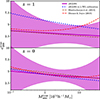 |
Fig. 9. Redshift evolution for the mass-concentration relation. The best-fit line and its 1σ uncertainty are shown as the magenta solid line and region, respectively. The blue dotted lines are the results without the WL calibration. The brown and red dashed lines denote the normalizations of numerical simulations of Bhattacharya et al. (2013) and Diemer & Joyce (2019), respectively. |
We divided the clusters into two subsamples using the number of peaks in the galaxy map. We selected clusters containing massive galaxy subhalos by applying the criterion that the ratio of the peak height of the most massive subhalo to that of the main cluster exceeds 0.5. We refer to these as multiple-peak clusters and the remaining clusters as single-peak clusters. In the analysis, we considered 75 association clusters, including those for which the WL masses have not been successfully measured, to focus on their average characteristics. The halo concentration for the multiple-peak clusters is  , which is about 0.63 times that of the single-peak clusters
  . The halo concentration for the single-peak clusters is in good agreement with the numerical simulations, while the result for the multiple-peak clusters is ∼3.5σ lower than those for the given mass. The two clusters (J141507.1-002905 and J141457.8-002050) in multiple-peak clusters are members of a three-cluster system. When we exclude the two clusters, the resulting
 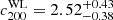 does not change significantly. This characteristic agrees with the lower concentration for merging clusters (e.g., Dutton & Macciò 2014; Klypin et al. 2016; Ishiyama et al. 2021). The same result was reported in optically selected clusters (Okabe et al. 2019).
3.6. Miscentering effect from 2D WL analysis
In the 2D analysis, the central positions are treated as a free parameter, allowing the calculation of the distance between the eRASS1 centroids and WL-determined centers, which offers crucial insights into the mis-centering effect. Since the S/N of the WL signals is not high enough (Fig. 1), the centers and masses of some clusters are not well determined from the marginalized posterior distributions. If the WL-determined centers are associated with other clusters, we removed them from the results. The sample of the 2D WL analysis using the spherical NFW model is limited to 36 clusters. The S/N of the lensing signal of the 36 clusters is S/N ≳ 4, with mean and median values of 5.4 and 5.1, respectively, belonging to a high S/N population in the parent samples (Sect. 3.2).
Figure 10 shows the probability distribution of the best-fit distance from the eRASS1 centroids. The errors are estimated by randomly drawing from the posterior distributions. The distribution has a peak around  and a tail at larger distances. To quantify the distribution, we introduced a model composed of two Gaussian components (Rayleigh distributions), as done in previous studies (Oguri et al. 2010, 2018; Ota et al. 2023):
![Mathematical equation: $$ \begin{aligned} \frac{dP}{dr}= f_{\rm cen}p_1(r)+(1-f_{\rm cen})p_2, p_i(r)=\frac{r}{\sigma _i^2}\exp \left[-\frac{r^2}{2r\sigma _i^2}\right]. \end{aligned} $$](/articles/aa/full_html/2025/08/aa53708-25/aa53708-25-eq117.gif) (22)
(22)
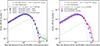 |
Fig. 10. Left: Best-fit distance from the eRASS1 centroids. The blue diamonds, green down-triangles, and magenta up-triangles represent the results of the spherical NFW model, the elliptical NFW model, and the inclusion of the multiple spherical NFW components, respectively. The red solid line, the light-blue dashed line, and the green dotted line are the best-fit for all the components, the inner Gaussian and the outer Gaussian, respectively. Right: Magenta up-triangles represent the distance from galaxy map peaks. The blue diamonds are the same as in the left panel. |
Here, fcen is the fraction of the inner Gaussian and σi is a scale parameter (standard error). Since there are the measurement uncertainties of the WL-determined centers, we convolved the function (Eq. (22)) with the typical measurement error of  . The best-fit result is shown in Table 3. The scale parameters of the inner and outer components are at most
  and
and  , respectively.
Parameters of the miscentering effect.
Due to the presence of several mass structures within certain cluster fields, we additionally conducted a multi-component analysis. Compared to the result of the single NFW model, J141457.8-002050 and J141507.1-002905 (Fig. 3) are added to the result. The probability distribution for the multiple-halo model is almost the same as that for the single-halo model (left panel of Fig. 10). The probability distribution for the single elliptical NFW model is also similar to those used for the single and multiple NFW models. The best-fit results do not change. However, the errors for the two clusters become 103 times larger and the tail over  is found (left panel of Fig. 10). Therefore, the WL centers do not change significantly with a choice of mass models and the miscentering effect is small.
We also computed the probability distribution for the single NFW model centering the peaks in the galaxy maps, as shown in the right panel of Fig. 10 and Table 3. The scale parameter of the inner component is about three times higher than that for the X-ray centroids. It shows that the X-ray centroids are a better tracer of the mass centers than the center of optical galaxies, thanks to the X-ray emissivity of ne2.
3.7. Stacked mass map
Since the measurement of mis-centering effect by the 2D WL analysis is limited to clusters with high WL S/N (Sect. 3.6), the effect is unclear for clusters with low WL S/N. We make stacked mass maps for the subsamples (Fig. 11), centering the eRASS1 X-ray centroids to visually investigate the mis-centering effect. The smoothing FWHM is 1 arcmin. The top three rows of Fig. 11 show the S/N maps for different bins of richness, redshift, and S/N in the tangential shear profile, respectively. The subsamples do not include the poor-fit or misassociation clusters. The central region above 6σ has an almost concentric distribution. All of the peak centers coincide with the X-ray centroids within the smoothing scale. The average redshifts are about the same at ∼0.2, suggesting a similar lensing efficiency. The peak S/N increases with increasing richness and WL S/N, as expected from the mass-richness correlation described in Sect. 3.4. The peak S/N in the redshift bins is highest at 0.2 ≤ z < 0.4, due to good lensing efficiency and a larger number of background galaxies. The peak SN for the poor-fit clusters has only a ∼3.6σ peak and no clear concentration. Even when we remove the substructure of the multiple-component cluster, J141457.8-002050 (Fig. 3), the result does not change significantly. The SN map for the misassociation clusters shows no lensing signal.
We compare the peak S/N ((S/N)peak) in the mass maps with the S/N in the stacked tangential shear ((S/N)⟨ΔΣ + ⟩) in the range of 100–3000  . They are highly correlated for the S/N subsamples ln(S/N)peak = 1.06 + 0.91ln(S/N)⟨ΔΣ + ⟩. The subsample with S/N < 4, which could not be analyzed in the 2D WL, has a peak height similar to that expected from the S/N of the other two subsamples. Therefore, by analogy with the results of the 2D WL analysis of the other two samples, a subsample with S/N < 4 would have a similar level of mis-centering effect as the result of the 2D WL analysis.
The peak height is also weakly correlated with the cluster richness ⟨λ⟩; ln(S/N)peak = 8.40 + 0.15ln⟨λ⟩. All the peaks expected from the richness are consistent with each other.
In contrast, the peak height of the poor-fit clusters is only 60 and 30 percent of those expected from (S/N)ΔΣ+ ≃ 4.1 and ⟨λ⟩≃30, respectively. As a result, the mass distribution of clusters with poor fits significantly differs from that of the remaining 63 clusters.
3.8. Poor-fit clusters
3.8.1. WL mass measurements
Both the stacked tangential shear profile (Fig. 6) and the stacked mass map (Fig. 11) for the 12 poor-fit clusters have different characteristics from the other 63 association clusters. Here, the 12 poor-fit clusters are composed of 5 clusters including J141457.8-002050 (Fig. 3) at z < 0.2, 5 clusters at 0.2 < z < 0.5, and 2 clusters at 0.5 < z, respectively. Since the lensing-weighted redshift is ⟨z⟩ = 0.19, these average lensing properties are affected by the clusters at z < 0.2 because the number of background galaxies at z > 0.4 is much smaller than that at z < 0.2. Since the mass parameters of the subsamples split by redshifts are poorly constrained and their difference is not statistically significant, we examined the average characteristics for the poor-fit clusters.
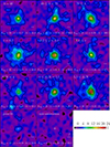 |
Fig. 11. S/N of stacked mass maps for the subsamples (12′×12′). The black contours represent the reconstructed WL mass map spaced in units of 2σ bootstrapping error starting from 2σ. The first, second, and third rows from the top show the maps for the subsamples divided by richness, redshift, and the S/N in the tangential shear, respectively. These samples exclude the poor-fit and misassociation clusters. The left and right panels in the bottom row show the mass maps for the poor-fit and misassociation clusters, respectively. The selection criteria are described in the upper part of each panel. The white crosses denote the eRASS1 centroids. The white horizontal line corresponds to the smoothing FWHM of 1′. The number of clusters, the average redshift, and the average richness are described in the lower part of each panel. |
When we fit the stacked tangential shear profile with a single NFW model, we obtain the extremely low concentration parameter of 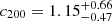 (Figs. 12 and 13). Indeed, the best-fit line is lower than the lensing signal observed in the central region of
 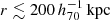 . To understand the discrepancy, we first add the point source at the center to the lensing model, but the best-fit point mass is too massive
  and the concentration parameter remains below 1. Since the lensing signals in the intermediate radius are low, the lensing profiles might be affected by the surrounding mass structures. Since the lensing signals for the poor-fit clusters are relatively low, we cannot identify the mass structure in the individual mass maps or find the eRASS1 clusters around the poor-fit clusters, except for J141457.8-002050 (Fig. 3). Therefore, we instead used the galaxy maps as a proxy to compute the lensing signal from the surrounding halos. We fixed the multi-halo positions and the best-fit WL masses for J141457.8-002050 obtained by 2D WL analysis and the offset positions of the galaxy peaks. The surrounding halos are distributed over
  for six clusters. The lensing-weighted average of the distance is
  . We parameterize the average mass associated with the galaxy peaks. Here, we assume that all the masses for the galaxy peaks are the same. Taking into account lensing weight in the stacked tangential shear profile, we computed the lensing signal from the surrounding halos as a function of M200, where c200 = 4 or c500 = 2.6 is fixed. The modeled tangential shear profiles are computed by synthesizing the NFW mass model of the main cluster and the surrounding halos.
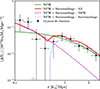 |
Fig. 12. Stacked tangential shear profile for the 12 poor-fit clusters (same as Fig. 6). The green solid line denotes the best-fit model for a single NFW model, but showing |

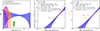 |
Fig. 13. Comparison of the baselines and the results of the poor-fit clusters. The green region and up-triangles are the results of the single NFW model for the 12 poor-fit clusters. The magenta region and squares are the results of the eRASS1 clusters considering the surrounding mass halos in the model fitting. The gray circles are the results of the total components, including the surrounding mass. The orange region and down-triangles are the results of the single NFW model for the six poor-fit clusters with a single galaxy peak. Left: Mass-concentration relation. Middle: Mass and the corrected CR relation. Right: Mass and richness relation. The lensing contribution from the surrounding halos cannot be ignored for the poor-fit clusters. Once we consider the surrounding halos, the concentration agrees with the baseline, but the masses expected from the count-rate or the richness are significantly overestimated. |
The constraints on the NFW parameters are weak, but not in contradiction with the baseline (left panel of Fig. 13). The halo masses for the main cluster and its surroundings are  and
and  , respectively. Given the masses, we obtain
 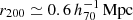 and
and 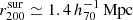 , respectively. Since the lensing-weighted average of the offset distances of the surrounding structures is
  , r200 slightly overlaps with each other. We rerun fitting for the 5 multi-halo clusters (excluding J141457.8-002050), and obtain
  and
and  , respectively. The results do not change significantly. Since the surrounding halos are more massive than the eRASS1 clusters, the eRASS1 clusters are likely to be subhalos or halos accompanied by the surrounding halos. We note that the surrounding structures are not listed by the main eRASS1 X-ray catalog (Merloni et al. 2024) except for J141457.8-002050. As for the single-peak clusters, we obtained a slightly higher mass of
  , along with
  .
.
As mentioned above, the poor-fit clusters are less massive objects at  . They are categorized into two categories: one includes structures with surrounding mass structures, while the other comprises those without. As for the clusters without the surrounding mass structures, the S/N in the stacked lensing profile is only 3.4. The WL mass measurements for these clusters are difficult simply because of the less massive objects. As for the clusters with the surrounding mass structures, the S/N in the stacked lensing profile is 9.4 but the lensing contamination from the surrounding structures cannot be ignored.
3.8.2. Scaling relations
We computed the stacked λ and the corrected CR for the 12 poor-fit clusters. The WL masses taken with and without the surrounding halos are shown by magenta squares and green triangles in Fig. 13. In the mass-CR relation, the WL masses estimated with and without the surroundings are ∼8σint and ∼4σint lower than those expected from the CR, respectively. Here, σint = σCR/βCR is the intrinsic scatter for the mass. Similarly, in the mass-richness relation, the WL masses with and without the surroundings are ∼7σint and ∼3σint lower, where σint = σλ/βλ. These results are similar to the results of the stacked mass maps showing the different mass distribution (Sect. 3.7). When we consider the total mass derived by modeling the eRASS1 clusters along with the surrounding mass structures, we find that the mass is marginally above the expectation from the mass-CR baseline, yet it aligns well with the expectation from the mass-λ baseline. This suggests that although galaxies within the surrounding structures are included in the richness calculation, the centrally concentrated X-ray count-rate is excluded from the surrounding mass structure.
This result highlights the importance of taking the surrounding mass structure into account when dealing with less massive clusters, for WL mass measurements, richness estimations, and X-ray count-rate analyses.
3.9. 2D halo ellipticity
The probability distribution of the 2D halo ellipticity (ε) measured by the 2D WL analysis is shown in Fig. 14. The number of clusters is 34. The errors are estimated by 50 000 Monte Carlo redistribution of the ellipticity parameter of each cluster. The average and median ellipticities are 0.45 and 0.47, respectively. The average measurement error for each cluster is 0.29. The probability distribution is slightly skewed; the probability at the lowest ellipticity bin is 1.4 times higher than that at the highest ellipticity bin. This is because we considered avoiding the zero bound by treating the absolute value but do not the bound at ε = 1. It is, therefore, difficult to conclude whether the skewed distribution is intrinsic or is due to the measurement technique. We fit the Gaussian distribution by convolving the average measurement error and obtain the mean ellipticity, 0.47, and the standard error 0.16.
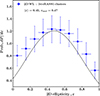 |
Fig. 14. 2D halo ellipticity distribution. The solid line is the best-fit Gaussian distribution convolved with the average measurement error. |
We simultaneously obtained the orientation angle with measurement error of a few percent. The small errors enable us to make a stacked mass map aligning the major axis with the y-axis (Fig. 15), which gives a sanity check to our measurement. We adopted X-ray centroids as the center. Since the miscentering effect is small, the choice of centers does not change the result. The 2D mass distribution is elongated along the y-axis, as expected by the 2D WL analysis. The degree and orientation angle of the elongation in the model-independent mass map are consistent with the result derived through the elliptical NFW model using discrete shear data. As a control sample, we made a stacked mass map with random orientations as shown in the top panel of Fig. 15. The mass distribution is almost concentric, in contrast to the aligned mass map.
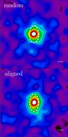 |
Fig. 15. Stacked mass maps for the 34 clusters analyzed with the elliptical NFW model. Top: Random orientations. Bottom: Aligned the major axis with the y-axis. The white dashed lines are auxiliary lines reflecting the median ellipticity. The white solid lines at the bottom right represent the 1 arcmin smoothing scale. |
We stacked eRASS1 soft-band (0.6–2.3 keV) images aligned with the major axis obtained by the 2D NFW fitting. We made X-ray images for individual clusters by subtracting the corresponding backgrounds and dividing them by the exposure maps. Here, we did not consider Galactic absorption at each cluster field because the clusters are located in a low Galactic column density region. We excluded X-ray images within 30 arcsec from X-ray point-sources in the main eRASS1 X-ray catalog (Merloni et al. 2024). The stacking weight, expressed in Eq. (16), was used to standardize the flux to its expectation at the average redshifts (zp = 0.19) of the 34 clusters. The resulting map is shown in the top panel of Fig. 16. We fit it with an elliptical β model; SX = S0(1 + (r/rc)2)−2β + 0.5 where r is an iso-contour computed with the ellipticity (Eq. (15)) and obtain the ellipticity εX ≃ 0.1. As expected, the best-fit major axis is aligned along the y axis. We stack the red galaxy maps, as shown in the bottom panel of Fig. 16. We fit it with the elliptical β model added to a background component and obtain ellipticity εG ≃ 0.1. When we use the galaxy map within 1 arcmin, the ellipticity becomes slightly higher εG ≃ 0.2. The best-fit major axis is aligned with the y-axis. Thus, the ellipticities of the hot and cold baryonic components are smaller than that of the mass (mainly dark matter) component.
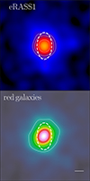 |
Fig. 16. Stacked eRASS1 (top) and galaxy (bottom) maps for the 34 clusters analyzed with the elliptical NFW model. The alignment is the same as Fig. 15. The white dashed lines are auxiliary lines reflecting the median ellipticity. The white solid lines at the bottom right represent the 1 arcmin smoothing scale. |
4. Discussion
4.1. Mass-richness-CR relation comparison
Figure 7 shows the baselines of eRASS1 (red dotted line; Ghirardini et al. 2024), eRASS-DES (green dot-dashed line; Grandis et al. 2024) and eFEDS (orange dashed line; Chiu et al. 2022) clusters. The mass-dependent slopes for the CR and the richness,  and
and 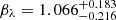 , are consistent with the slope in the soft-band X-ray luminosity and mass relation (LsoftX ∝ M) and the idea that the number of cluster members is proportional to the cluster masses. In contrast, our constraints on δ in the mass-dependent slope are poor due to the small number of our sample, while the literature (Chiu et al. 2022; Ghirardini et al. 2024; Grandis et al. 2024) constrains it well. Therefore, we computed the mass-dependent slopes in the literature (Chiu et al. 2022; Ghirardini et al. 2024; Grandis et al. 2024) at our lensing-weighted average redshift (zp = 0.21) for the following comparison. As the error covariance matrix for regression parameters is not fully detailed in the literature, we opted for the best-fit baseline. This choice does not impact the following discussion because our measurement errors are larger than those reported in the literature.
The best-fit slope of the mass-CR scaling relation is 1 ∼ 2σ lower than βCR = 1.69 (Chiu et al. 2022), βCR = 1.42 (Ghirardini et al. 2024) and βCR = 1.71 (Grandis et al. 2024). The intrinsic scatter of the count rate, 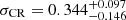 , is comparable to the eFEDS-HSC result of
 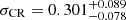 (Chiu et al. 2022), while
 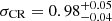 (Ghirardini et al. 2024) and σCR = 0.61 ± 0.19 (Grandis et al. 2024) are more than twice as large as ours. Ghirardini et al. (2024) discussed the very large intrinsic scatter by introducing the mass-dependent slope in the intrinsic scatter and contamination of the active galactic nuclei and random sources. We concluded that a further study is needed to understand the causes of very large intrinsic scatter. Ultimately, we did not find such a large intrinsic scatter in the eFEDS-HSC and eRASS1-HSC analyses.
Our result of the mass and richness scaling relation agrees with the results of eRASS1 (Ghirardini et al. 2024) and eFEDS (Chiu et al. 2022), although the richness measurement of (Ghirardini et al. 2024) is different. Our mass-dependent slope agrees well with βλ = 0.98 (Ghirardini et al. 2024) and βλ = 0.94 Chiu et al. (2022). The intrinsic scatter of the richness,  , agrees well with
  Chiu et al. (2022) and
  (Ghirardini et al. 2024).
4.2. Miscentering effect
The results of the 2D WL analysis (Sect. 3.6) show that the probability distribution of the offset distance (Fig. 10) is composed of a double peak structure. The standard error (scale parameter) of the inner component of the X-ray centroids is at most  , which indicates that the X-ray centroids are a good tracer of the bottom of the gravitational potential projected on to the sky.
To confirm this result independently, we also fit the stacked lensing profile for the 36 clusters used in the 2D WL analysis and the 75 association clusters with the mis-centering NFW model. We chose X-ray centroids as the centers. Here we assume that the concentration parameter follows Diemer & Joyce (2019) and that the offset distances, doff, are the same for all the clusters. In other words, the fitting procedure determines doff to represent the concentration parameter (Diemer & Joyce 2019). We used the flat prior, ![Mathematical equation: $ [\ln 0.02, \ln 0.5]\,h_{70}^{-1}\,\mathrm{Mpc} $](/articles/aa/full_html/2025/08/aa53708-25/aa53708-25-eq156.gif) , for lndoff. We obtained
, for lndoff. We obtained  and
and  for the 36 and 75 association clusters, respectively. They are consistent with the result obtained in the 2D WL analysis. Therefore, the miscentering effect with the X-ray centroids is, on average, negligible when describing the lensing properties.
The scale parameter of the inner component using the galaxy peaks,  , is about three times larger than that using the X-ray centroids. In the stacked lensing analysis, we chose the innermost radius as
  , the miscentering effect would appear in the concentration parameter derived by the stacked lensing analysis. We repeated the stacked lensing analysis for the 36 clusters used in the 2D WL analysis using the galaxy peaks and obtained
  , which is about ∼12.7% lower than that using the eRASS1 centroids. The discrepancy is at the 1σ uncertainty level. Similarly, we computed the stacked lensing profiles for the 27 non-poor-fit clusters that were not suitable for study using the 2D WL analysis. The resulting concentration parameters using the galaxy peak centers and the eRASS1 centroids agree within the error. Hence, it is difficult to identify that the galaxy peaks are statistically more misaligned than the eRASS1 centroids for the less massive clusters.
We calculated the distance between galaxy peaks and the eRASS1 X-ray centroids. The resulting parameters of the 75 association clusters are 
 , and
, and  . The resulting parameters of the 36 clusters used in the 2D WL analysis are similar to those for the 75 association clusters. Interestingly, the scale parameter of the inner component is smaller than that of the inner one between the WL-determined centers and galaxy peaks. Figure 17 presents a comparison of the deconvolved separations among three distinct components. The X-ray centroids are the best tracer of the WL centers. The directions in which the galaxy peaks are offset from the eRASS1 centroids differ from the offset directions of the WL centers. As a result, the offset distance between the WL centers and the galaxy peaks is the largest.
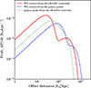 |
Fig. 17. Offset distances between the WL centers and the eRASS1 centroids (red solid line), between the WL centers and the galaxy peaks (blue dashed line), and between the galaxy peaks and the eRASS1 centroids (green dotted line). It indicates that the offset directions of the galaxy peaks are different from those of the WL centers. |
Among the 12 poor-fit clusters, 6 clusters have surrounding halos. The average mass for the surrounding halos is more massive than that for the eRASS1 clusters (Sect. 3.8). Since these surrounding structures, except for J141457.8-002050, are not identified by X-ray, it causes a possible source of mis-centering effect. We computed the probability distribution of the offset distance (Fig. 10) including the five poor-fit clusters accompanied by the undetected surrounding structures, assuming that the true centers are in the surrounding halos and their uncertainty of the center determination is the mean value obtained by the 2D WL analysis. The scale parameters, σ1 and σ2 (Eq. (22)), change by only ∼ + 5 and ∼ + 7%, respectively. Therefore, the mis-centering effect is statistically small in the whole sample.
Chiu et al. (2022) have computed the offset distribution between X-ray centroids and optical BCGs for the 313 eFEDS clusters and characterize it by a combination of a Rayleigh distribution for the outer component and a modified Rayleigh distribution for the inner component. The best-fit scale parameters for the inner and outer components are  and
and  , and the fraction for the inner component is fcen = 1 − 0.54 ± 0.02 = 0.46 ± 0.02. These parameters for the outer component are used as Gaussian priors for a simultaneous WL fit. The scale parameters are larger than our results between the galaxy peaks and the eRASS1 centroids. It might be due to the following feature that the galaxy peaks are insensitive to bright galaxies but sensitive to the number of member galaxies.
Grandis et al. (2024) have studied an intrinsic miscentering using the hydrodynamical cosmological simulations. With 100 random viewing angles for the simulated 191 clusters (116 clusters at z = 0.252 and 75 clusters at z = 0.518), the offset between the peak of X-ray surface brightness distribution in 0.5–2 keV and the center-of-mass on the sky is well described by a single Rayleigh distribution with mean  and σint = 0.104 ± 0.016. Given the mean value, we obtain the scale parameter,
  and
and  when we insert r500 for our sample. They also studied the observational miscentering effect using the offset between input and output position of clusters in the “eROSITA all-sky survey twin” Seppi et al. (2022). Taking into account a realistic active galactic nucleus and cluster properties under the eRASS1 observational conditions, they obtained a typical miscentering ∼11 arcsec (see Sect. 4.2.2 in Grandis et al. 2024). They synthesized the two miscentering effects in the WL mass measurement. Their miscentering effect corresponds to our inner component.
Ota et al. (2023) studied the offset distribution between X-ray centroids and NFW-determined centers by 2D WL analysis for the 23 HSC-CAMIRA clusters (Oguri et al. 2018) of which richness is higher than N > 40 in the eFEDS field. They obtained  ,
,  and fcen = 0.56 for X-ray centroids of the CAMIRA clusters, where they did not consider the typical measurement errors for the WL centers. We refit it with the double-peak structure convolved with the typical measurement error of
  and obtain
 and
and  . The scale parameter of the inner component is similar to ours. However, the scale parameter of the outer component is seven times larger than ours. It might be caused by the fact that they did not check whether the WL-determined centers belong to other clusters. The scale parameters of the inner component from the CAMIRA centers and the galaxy peaks are
  and
and  , respectively. Similarly, the central positions identified by galaxies are further away from the WL centers.
Melchior et al. (2017) carried out the WL mass calibration of redMaPPer clusters, using the DES Science Verification field. They compared the centers of the redMaPPer clusters with X-ray data and SZ data from the South Pole Telescope. They considered the uncertainty of the X-ray and SZ centers (Rykoff et al. 2016) and found that the fraction of the central component is fcen = 0.76 and the scale parameter is about 35% of the cluster radius determined by richness. Their results are similar to what we found in our study.
Bocquet et al. (2024) evaluated the miscentering effect by combining the optical data of the DES and the Hubble Space Telescope and the SZ data from the South Pole Telescope. The central fractions for the SZ and optical distributions are 0.88 and 0.89. The scale parameters for the optical distribution are  and
and  . The SZ distribution has similar properties. They also investigate the mis-centering effect using 70 clusters from Chandra X-ray data and found fcen = 0.8,
  and
and  . Their results are similar to our findings from the 2D WL analysis.
4.3. Background selection
The main systematics of cluster mass measurements is a background selection. If cluster members are included in the shape catalog, the concentration parameter, c200, or the masses, MΔ (Δ ≳ 500), within inner radii, are underestimated because the fraction of member galaxies to background galaxies increases with decreasing radius. The effect is known as a dilution effect (e.g., Broadhurst et al. 2005; Umetsu et al. 2014; Okabe & Smith 2016; Ziparo et al. 2016; Medezinski et al. 2018). Historically, the number of available imaging bands was limited, and background galaxies were selected in the color-magnitude plane (Okabe & Smith 2016) or the color-color plane (Umetsu et al. 2014), which is referred to as the color-color (CC) selection. The advantage of the CC selection is independent of the photometric redshifts. In the multi-band survey era, background galaxies can be selected using photometric redshifts, which is referred to as the Pz selection.
Medezinski et al. (2018) have developed a new CC selection using the HSC five-band imaging through a monitor of colors and lensing signals. They also have found that the masses estimated with the CC and Pz selections are in good agreement. We repeat the same analysis using the CC selection as the Pz selection. A mass comparison is shown in Fig. 18. We perform a regression analysis with  and obtain
  and
and  . The intrinsic scatter is < 0.138. When we fix βCC, Pz = 1 and no intrinsic scatter, we obtain
  , that is, the weighted geometric mean of the mass ratio of
  . The masses of the two background selections are therefore in excellent agreement.
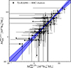 |
Fig. 18. Mass comparison with the Pz and CC selections. The blue solid line and the blue region are the best-fit and the 1σ uncertainty. |
4.4. Mass-concentration relation
As discussed in Sect. 4.2, the miscentering effect is statistically negligible and thus does not affect the estimation of the halo concentration. The mass and concentration relation for the eRASS1 clusters agrees well with the numerical simulations as shown in Fig. 8, which supports the assumptions of the mass-concentration relation adopted in the simultaneous WL mass measurements for the eRASS1 clusters (Chiu et al. 2022; Grandis et al. 2024; Kleinebreil et al. 2025).
Since the mass and concentration relation provides us with an opportunity to test hierarchical structure formation on a scale of Mpc, it has been relatively well investigated in previous studies. (Fig. 19; e.g., Umetsu et al. 2014, 2016, 2020; Okabe & Smith 2016; Cibirka et al. 2017; Sereno et al. 2017; Okabe et al. 2019). The cluster catalog of the ROSAT All Sky Survey (RASS; e.g., Voges et al. 1999; Böhringer et al. 2004) were used for the WL analyses (Umetsu et al. 2014, 2016; Okabe & Smith 2016; Cibirka et al. 2017). The Subaru/Suprime-cam WL analyses of CLASH (Umetsu et al. 2014, 2016) and LoCuSS (Okabe & Smith 2016) selected massive ROSAT clusters 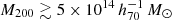 at a redshift slice z ∼ 0.2. Since the number densities of background galaxies are more than twice that of our paper, they did not apply WL calibration. They found a negative mass-dependent slope but could not constrain the redshift evolution because of narrow redshift ranges. Cibirka et al. (2017) measured stacked mass and concentration for 27 massive clusters
  at a redshift slice of z ∼ 0.5 using the Canada-France-Hawaii Telescope (CFHT) data. Using the HSC-SSP shape catalog, the XXL survey covers less massive clusters and groups, whose masses cover a range down to
  (Umetsu et al. 2020) in the wide redshift range of 0.031 ≤ z ≤ 1.033. Our result agrees well with the mass-concentration relation for the RASS clusters (Umetsu et al. 2014, 2016; Okabe & Smith 2016; Cibirka et al. 2017) and the XXL clusters (Umetsu et al. 2020). The concentration for the PSZ2 clusters from the Planck mission is somewhat lower than our concentration (Sereno et al. 2017).
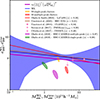 |
Fig. 19. Comparison with the literature. The blue solid line and the blue region are the best-fit and the 1σ uncertainty (Fig. 8), respectively. The magenta line is the true mass and concentration relation. The red and brown lines are the best-fit lines of Okabe & Smith (2016) and Umetsu et al. (2020), respectively, where the redshift zref = 0.3 of Umetsu et al. (2020) is converted to z = 0.21. The orange and red shaded regions represent the 1σ constraints by stacked lensing analysis for the 53 clusters with single galaxy peak, and the 22 clusters with multiple galaxy peaks, respectively. The green and pink shaded regions represent the 1σ constraints by stacked lensing analysis for the HSC-CAMIRA clusters (Okabe et al. 2019) with single galaxy peak and multiple galaxy peaks, respectively. The pink square, up-triangle and down-triangle are the results of stacked lensing analyses of Umetsu et al. (2016), Cibirka et al. (2017) and Sereno et al. (2017), respectively. |
As for optically selected clusters, (Okabe et al. 2019) performed a stacked lensing analysis for the HSC-CAMIRA clusters (Oguri et al. 2018) to compare the concentration parameter for the single and multiple peaks in the galaxy maps. They did not consider the miscentering effect in the mass modeling. The concentration parameter for the single-peak clusters is about 60% of the baseline. Since the mass measurement techniques are the same as our analysis, the miscentering effect for the optically selected clusters cannot be ignored, as found in Ota et al. (2023) and Sect. 4.2. in Okabe et al. (2019) have also shown that the halo concentration for the multiple-peak clusters is ∼33% lower than that for the single-peak clusters. Similar results are found in our analysis; the ratio between the concentration parameters for the eRASS1 clusters with multiple-peak and single-peak is ∼0.63.
The cluster catalog covering a wide redshift range enables us to measure the redshift evolution of normalization. (Umetsu et al. 2020) have shown the slope γ = −0.03 ± 0.47. Our result gives a similar result, namely,  . Since both measurement errors are still large, we need a larger sample of clusters over wide redshift ranges.
As shown in Fig. 8, the resulting baseline is in good agreement with dark matter-only numerical simulations (Bhattacharya et al. 2013; Child et al. 2018; Diemer & Joyce 2019; Ishiyama et al. 2021). Similar results have been reported in the literature (Umetsu et al. 2014, 2016; Okabe & Smith 2016; Cibirka et al. 2017). For instance, Child et al. (2018) have shown that the concentration parameter for the unrelaxed clusters is 69% of that for the relaxed clusters at z = 0. The feature is similar to our results. The redshift evolution is similar to the numerical simulations (Fig. 9). However, the concentration parameters of different numerical simulations at z = 1 vary by up to ≳50% at the high mass end. To further constrain the redshift evolution in future studies, we need a large number of clusters at high redshifts and carefully treat the WL mass bias caused by a small number of background galaxies.
4.5. 2D halo ellipticity
We do not adopt any WL mass calibration in the halo ellipticity measurement. We leave this as next task using numerical simulations.
Our result agrees well with ⟨ε⟩ = 0.46 ± 0.04 of the pilot 2D WL study (Oguri et al. 2010). Umetsu et al. (2018) measured 2D halo ellipticity for 20 high-mass galaxy clusters selected from the CLASH survey and found ⟨ε⟩ = 0.33 ± 0.07 at Mvir ≃ 1015 M⊙. They discussed the CLASH selection function based on X-ray morphological regularity, with its average value being slightly lower than theoretical predictions. Chiu et al. (2018) constrained the minor-to-major axis ratio to a mass scaling relation for the 20 CLASH clusters by a decomposition method using a strong and weak lensing dataset. Their result using the informative prior from dark matter simulations (Bonamigo et al. 2015) shows ⟨ε3D⟩≃0.50 at a stacked WL mass  for the 34 clusters measured with the elliptical NFW model. Their result is similar to ours. The findings impose constraints on the halo ellipticity within a mass range of about a half or less compared to previous studies; for example,
  (Oguri et al. 2010) and
  (Umetsu et al. 2018; Chiu et al. 2018). Although it is difficult to make a direct comparison with the 3D halo ellipticity, our results are similar to ε ∼ 0.45 − 0.55 from numerical simulations (Despali et al. 2014; Bonamigo et al. 2015; Bett et al. 2007).
Okabe et al. (2018) studied the projected ellipticity and orientation distributions for gas, stars, and dark matter using Horizon-AGN Simulation (Dubois et al. 2014). They found the mean projected ellipticities measured within 1 Mpc radius are 0.33 for the total mass, 0.48 for the galaxies, and 0.17 for the gas, respectively. Their findings are consistent with ours, except for the galaxies. Given that we stacked galaxies based on WL-determined orientations, any mis-centering between galaxies and mass could obscure the ellipticities of the stacked galaxies map. When we choose optical centers, the project ellipticity of the galaxies becomes εG ∼ 0.35, which marginally agrees with Okabe et al. (2018). Furthermore, if the orientation angles of different components are misaligned, our measurements of gas and galaxy ellipticities would be underestimated. Individual analysis for massive nearby clusters would be suitable for more detailed studies because of good statistics of photon and member counts.
4.6. eRASS1 mass comparison
We compared the individual WL masses with the eRASS1 masses (Bulbul et al. 2024). The eRASS1 masses have been computed with the posterior distributions obtained by a simultaneous fit for the target cluster with priors of count-rate and mis-centering effect under an assumption of the mass and concentration relation (Chiu et al. 2022; Grandis et al. 2024; Kleinebreil et al. 2025). It is important to compare masses in a complementary way to our analysis.
The number of clusters for the comparison is 76 in total because the two misassociation clusters, J114647.4-012428 and J124503.8-002823, are listed in the cosmology sample (Ghirardini et al. 2024), but not in the primary sample (Bulbul et al. 2024). Among them, the masses of four clusters, including a misassociation cluster and two poor-fit clusters, are not listed in the primary sample, and our analysis cannot measure the WL masses for the two clusters. Thus, the number of samples is 70 clusters. Figure 20 shows a mass comparison, showing a good agreement. We perform the regression analysis with no redshift evolution of the normalization. The mass ratio between  and
and  is shown in the bottom panel of Fig. 20. The baseline is consistent with unity within the 1σ level, though the best-fit value is −5% at
  and −5% at
  . As mentioned in Sect. 3.8, a treatment of surrounding halos at
  from the poor-fit clusters of which masses are
  is important. Even when we exclude the poor-fit clusters, the results do not change significantly. When we set the mass-dependent slope to unity, we obtain the ratio
  and
and  for all the clusters and the sample excluding the poor-fit clusters, respectively.
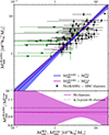 |
Fig. 20. Top: Mass comparison between |


5. Conclusions
In this work, we present the individual WL mass measurements for 78 eRASS1 clusters in the HSC-SSP footprint. In our analysis, we did not adopt any priors for the eRASS1 X-ray quantities and the richness and the assumption of the mass and concentration relation, which is complementary to other WL mass measurements employed for the eFEDS or eRASS1 clusters (Chiu et al. 2022; Grandis et al. 2024; Kleinebreil et al. 2025).
The cluster sample was selected from the 103 eRASS1 clusters within the HSC-SSP footprint in order to ensure a sufficient number of background galaxies were available. Specifically, clusters lacking a uniform azimuthal distribution of background galaxies were excluded. By visual inspection of the HSC-SSP optical images, we found that 3 out of the 78 eRASS1 clusters do not exhibit a match with the optical counterparts (Fig. 4). This finding was further supported by the null-lensing signal in its stacked lensing profile (Fig. 5).
Taking into account the WL mass calibration, the scaling relations between the true mass and cluster richness and X-ray count-rate are in good agreement with the results of the eRASS1 Western Galactic Hemisphere region based on count-rate-inferred masses, which have been calibrated with the HSC-SSP, DES, and KiDS surveys.
We developed a Bayesian framework to measure the true mass and concentration relation, considering the WL mass calibration in the mass and concentration plane. The redshift-dependent mass and concentration measurements are in excellent agreement with numerical simulations and previous studies.
Based on the 2D WL analysis, the offsets between the WL-determined centers and X-ray centroids for the 36 eRASS1 clusters with high WL S/N are described by two Gaussian components. The miscentering effect with the X-ray centroids is small, as also assumed in the previous studies (Chiu et al. 2022; Grandis et al. 2024). The stacked mass maps support it even for less massive clusters. In contrast, when we use the galaxy peaks, the miscentering effect becomes slightly larger.
The projected halo ellipticity driven by the 2D WL analysis shows ⟨ε⟩ = 0.45, which agrees with the results of numerical simulations and previous studies. The stacked mass map, aligned with the major axes, represents the elongated structure obtained from the 2D WL analysis. The optical and X-ray ellipticities are ε ≃ 0.1 − 0.2 and smaller than the result from the dark matter distribution.
The average mass for the 12 poor-fit clusters changes from  to
to  when lensing contamination from surrounding mass structures is taken into account. In that case, the concentration parameter is significantly improved from ∼1 by including lensing contamination. An accurate WL mass measurement would require the modeling procedure to include the surrounding halos or a choice of the maximum radius in the tangential shear profile.
Acknowledgments
The Hyper Suprime-Cam (HSC) collaboration includes the astronomical communities of Japan and Taiwan, and Princeton University. The HSC instrumentation and software were developed by the National Astronomical Observatory of Japan (NAOJ), the Kavli Institute for the Physics and Mathematics of the Universe (Kavli IPMU), the University of Tokyo, the High Energy Accelerator Research Organization (KEK), the Academia Sinica Institute for Astronomy and Astrophysics in Taiwan (ASIAA), and Princeton University. Funding was contributed by the FIRST program from the Japanese Cabinet Office, the Ministry of Education, Culture, Sports, Science and Technology (MEXT), the Japan Society for the Promotion of Science (JSPS), Japan Science and Technology Agency (JST), the Toray Science Foundation, NAOJ, Kavli IPMU, KEK, ASIAA, and Princeton University. This paper makes use of software developed for the Large Synoptic Survey Telescope. We thank the LSST Project for making their code available as free software at http://dm.lsst.org This paper is based [in part] on data collected at the Subaru Telescope and retrieved from the HSC data archive system, which is operated by Subaru Telescope and Astronomy Data Center (ADC) at NAOJ. Data analysis was in part carried out with the cooperation of Center for Computational Astrophysics (CfCA), NAOJ. We are honored and grateful for the opportunity of observing the Universe from Maunakea, which has the cultural, historical and natural significance in Hawaii. The Pan-STARRS1 Surveys (PS1) and the PS1 public science archive have been made possible through contributions by the Institute for Astronomy, the University of Hawaii, the Pan-STARRS Project Office, the Max Planck Society and its participating institutes, the Max Planck Institute for Astronomy, Heidelberg, and the Max Planck Institute for Extraterrestrial Physics, Garching, The Johns Hopkins University, Durham University, the University of Edinburgh, the Queen’s University Belfast, the Harvard-Smithsonian Center for Astrophysics, the Las Cumbres Observatory Global Telescope Network Incorporated, the National Central University of Taiwan, the Space Telescope Science Institute, the National Aeronautics and Space Administration under grant No. NNX08AR22G issued through the Planetary Science Division of the NASA Science Mission Directorate, the National Science Foundation grant No. AST-1238877, the University of Maryland, Eotvos Lorand University (ELTE), the Los Alamos National Laboratory, and the Gordon and Betty Moore Foundation. This work is based on data from eROSITA, the soft X-ray instrument aboard SRG, a joint Russian-German science mission supported by the Russian Space Agency (Roskosmos), in the interests of the Russian Academy of Sciences represented by its Space Research Institute (IKI), and the Deutsches Zentrum für Luft- und Raumfahrt (DLR). The SRG spacecraft was built by Lavochkin Association (NPOL) and its subcontractors, and is operated by NPOL with support from the Max Planck Institute for Extraterrestrial Physics (MPE). The development and construction of the eROSITA X-ray instrument was led by MPE, with contributions from the Dr. Karl Remeis Observatory Bamberg & ECAP (FAU Erlangen-Nuernberg), the University of Hamburg Observatory, the Leibniz Institute for Astrophysics Potsdam (AIP), and the Institute for Astronomy and Astrophysics of the University of Tübingen, with the support of DLR and the Max Planck Society. The Argelander Institute for Astronomy of the University of Bonn and the Ludwig Maximilians Universität Munich also participated in the science preparation for eROSITA. N. Okabe and M. Oguri acknowledge JSPS KAKENHI Grant Number JP19KK0076. K.U. acknowledges support from the National Science and Technology Council of Taiwan (grant NSTC 112-2112-M-001-027-MY3) and the Academia Sinica Investigator Award (grant AS-IA-112-M04). E. Bulbul, A. Liu, V. Ghirardini, and X. Zhang acknowledge financial support from the European Research Council (ERC) Consolidator Grant under the European Union’s Horizon 2020 research and innovation program (grant agreement CoG DarkQuest No 101002585). VG acknowledges the financial contribution from the contracts Prin-MUR 2022 supported by Next Generation EU (M4.C2.1.1, n.20227RNLY3 The concordance cosmological model: stress-tests with galaxy clusters). This paper is dedicated to our late friend, Dr. Yuying Zhang, who had hoped to pursue research using eROSITA and to contribute to the eROSITA–HSC collaboration, but sadly passed away before this could be realized; we will always cherish our shared aspirations.
References
- Abell, G. O. 1958, ApJS, 3, 211 [NASA ADS] [CrossRef] [Google Scholar]
- Aguado, D. S., Ahumada, R., Almeida, A., et al. 2019, ApJS, 240, 23 [Google Scholar]
- Aihara, H., Arimoto, N., Armstrong, R., et al. 2018, PASJ, 70, S4 [NASA ADS] [Google Scholar]
- Aihara, H., AlSayyad, Y., Ando, M., et al. 2022, PASJ, 74, 247 [NASA ADS] [CrossRef] [Google Scholar]
- Akino, D., Eckert, D., Okabe, N., et al. 2022, PASJ, 74, 175 [NASA ADS] [CrossRef] [Google Scholar]
- Artis, E., Ghirardini, V., Bulbul, E., et al. 2024, A&A, 691, A301 [NASA ADS] [CrossRef] [EDP Sciences] [Google Scholar]
- Artis, E., Bulbul, E., Grandis, S., et al. 2025, A&A, 696, A5 [NASA ADS] [CrossRef] [EDP Sciences] [Google Scholar]
- Baldry, I. K., Liske, J., Brown, M. J. I., et al. 2018, MNRAS, 474, 3875 [Google Scholar]
- Becker, M. R., & Kravtsov, A. V. 2011, ApJ, 740, 25 [NASA ADS] [CrossRef] [Google Scholar]
- Bett, P., Eke, V., Frenk, C. S., et al. 2007, MNRAS, 376, 215 [NASA ADS] [CrossRef] [Google Scholar]
- Bhattacharya, S., Habib, S., Heitmann, K., & Vikhlinin, A. 2013, ApJ, 766, 32 [Google Scholar]
- Bocquet, S., Grandis, S., Bleem, L. E., et al. 2024, Phys. Rev. D, 110, 083509 [NASA ADS] [CrossRef] [Google Scholar]
- Böhringer, H., Schuecker, P., Guzzo, L., et al. 2004, A&A, 425, 367 [NASA ADS] [CrossRef] [EDP Sciences] [Google Scholar]
- Bonamigo, M., Despali, G., Limousin, M., et al. 2015, MNRAS, 449, 3171 [NASA ADS] [CrossRef] [Google Scholar]
- Broadhurst, T., Takada, M., Umetsu, K., et al. 2005, ApJ, 619, L143 [NASA ADS] [CrossRef] [Google Scholar]
- Bulbul, E., Chiu, I. N., Mohr, J. J., et al. 2019, ApJ, 871, 50 [Google Scholar]
- Bulbul, E., Liu, A., Kluge, M., et al. 2024, A&A, 685, A106 [NASA ADS] [CrossRef] [EDP Sciences] [Google Scholar]
- Bullock, J. S., Kolatt, T. S., Sigad, Y., et al. 2001, MNRAS, 321, 559 [Google Scholar]
- Carrasco Kind, M., & Brunner, R. J. 2014, MNRAS, 438, 3409 [NASA ADS] [CrossRef] [Google Scholar]
- Child, H. L., Habib, S., Heitmann, K., et al. 2018, ApJ, 859, 55 [NASA ADS] [CrossRef] [Google Scholar]
- Chiu, I. N., Umetsu, K., Sereno, M., et al. 2018, ApJ, 860, 126 [NASA ADS] [CrossRef] [Google Scholar]
- Chiu, I. N., Ghirardini, V., Liu, A., et al. 2022, A&A, 661, A11 [NASA ADS] [CrossRef] [EDP Sciences] [Google Scholar]
- Chiu, I. N., Klein, M., Mohr, J., & Bocquet, S. 2023, MNRAS, 522, 1601 [NASA ADS] [CrossRef] [Google Scholar]
- Chiu, I.-N., Ghirardini, V., Grandis, S., et al. 2025, A&A, submitted [arXiv:2504.01076] [Google Scholar]
- Cibirka, N., Cypriano, E. S., Brimioulle, F., et al. 2017, MNRAS, 468, 1092 [Google Scholar]
- Clerc, N., Comparat, J., Seppi, R., et al. 2024, A&A, 687, A238 [NASA ADS] [CrossRef] [EDP Sciences] [Google Scholar]
- Colless, M., Peterson, B. A., Jackson, C., et al. 2003, ArXiv e-prints [arXiv:astro-ph/0306581] [Google Scholar]
- Despali, G., Giocoli, C., & Tormen, G. 2014, MNRAS, 443, 3208 [Google Scholar]
- Diemer, B., & Joyce, M. 2019, ApJ, 871, 168 [NASA ADS] [CrossRef] [Google Scholar]
- Diemer, B., & Kravtsov, A. V. 2015, ApJ, 799, 108 [Google Scholar]
- Dietrich, J. P., Erben, T., Lamer, G., et al. 2007, A&A, 470, 821 [NASA ADS] [CrossRef] [EDP Sciences] [Google Scholar]
- Dubois, Y., Pichon, C., Welker, C., et al. 2014, MNRAS, 444, 1453 [Google Scholar]
- Dutton, A. A., & Macciò, A. V. 2014, MNRAS, 441, 3359 [Google Scholar]
- Euclid Collaboration (Giocoli, C., et al.) 2024, A&A, 681, A67 [NASA ADS] [CrossRef] [EDP Sciences] [Google Scholar]
- Gal, R. R., Lopes, P. A. A., de Carvalho, R. R., et al. 2009, AJ, 137, 2981 [NASA ADS] [CrossRef] [Google Scholar]
- Ghirardini, V., Bulbul, E., Artis, E., et al. 2024, A&A, 689, A298 [NASA ADS] [CrossRef] [EDP Sciences] [Google Scholar]
- Giocoli, C., Meneghetti, M., Ettori, S., & Moscardini, L. 2012, MNRAS, 426, 1558 [NASA ADS] [CrossRef] [Google Scholar]
- Golse, G., & Kneib, J. P. 2002, A&A, 390, 821 [NASA ADS] [CrossRef] [EDP Sciences] [Google Scholar]
- Goto, T., Sekiguchi, M., Nichol, R. C., et al. 2002, AJ, 123, 1807 [NASA ADS] [CrossRef] [Google Scholar]
- Grandis, S., Ghirardini, V., Bocquet, S., et al. 2024, A&A, 687, A178 [NASA ADS] [CrossRef] [EDP Sciences] [Google Scholar]
- Heymans, C., Van Waerbeke, L., Bacon, D., et al. 2006, MNRAS, 368, 1323 [Google Scholar]
- Hilton, M., Sifón, C., Naess, S., et al. 2021, ApJS, 253, 3 [Google Scholar]
- Hirata, C., & Seljak, U. 2003, MNRAS, 343, 459 [Google Scholar]
- Ishiyama, T., Prada, F., Klypin, A. A., et al. 2021, MNRAS, 506, 4210 [NASA ADS] [CrossRef] [Google Scholar]
- Kaiser, N., & Squires, G. 1993, ApJ, 404, 441 [Google Scholar]
- Klein, M., Oguri, M., Mohr, J. J., et al. 2022, A&A, 661, A4 [NASA ADS] [CrossRef] [EDP Sciences] [Google Scholar]
- Kleinebreil, F., Grandis, S., Schrabback, T., et al. 2025, A&A, 695, A216 [NASA ADS] [CrossRef] [EDP Sciences] [Google Scholar]
- Kluge, M., Comparat, J., Liu, A., et al. 2024, A&A, 688, A210 [NASA ADS] [CrossRef] [EDP Sciences] [Google Scholar]
- Klypin, A., Yepes, G., Gottlöber, S., Prada, F., & Heß, S. 2016, MNRAS, 457, 4340 [Google Scholar]
- Koester, B. P., McKay, T. A., Annis, J., et al. 2007, ApJ, 660, 239 [NASA ADS] [CrossRef] [Google Scholar]
- Li, X., Miyatake, H., Luo, W., et al. 2022, Publ. Astron. Soc. Jpn., 74, 421 [Google Scholar]
- Lilly, S. J., Le Brun, V., Maier, C., et al. 2009, ApJS, 184, 218 [Google Scholar]
- Liu, A., Bulbul, E., Ghirardini, V., et al. 2022, A&A, 661, A2 [NASA ADS] [CrossRef] [EDP Sciences] [Google Scholar]
- Mandelbaum, R., Hirata, C. M., Seljak, U., et al. 2005, MNRAS, 361, 1287 [Google Scholar]
- Mandelbaum, R., Rowe, B., Bosch, J., et al. 2014, ApJS, 212, 5 [Google Scholar]
- Mandelbaum, R., Rowe, B., Armstrong, R., et al. 2015, MNRAS, 450, 2963 [Google Scholar]
- Mandelbaum, R., Miyatake, H., Hamana, T., et al. 2018a, PASJ, 70, S25 [Google Scholar]
- Mandelbaum, R., Lanusse, F., Leauthaud, A., et al. 2018b, MNRAS, 481, 3170 [NASA ADS] [CrossRef] [Google Scholar]
- Massey, R., Heymans, C., Bergé, J., et al. 2007, MNRAS, 376, 13 [Google Scholar]
- McCarthy, I. G., Schaye, J., Bird, S., & Le Brun, A. M. C. 2017, MNRAS, 465, 2936 [Google Scholar]
- Medezinski, E., Oguri, M., Nishizawa, A. J., et al. 2018, PASJ, 70, 30 [NASA ADS] [Google Scholar]
- Mehrtens, N., Romer, A. K., Hilton, M., et al. 2012, MNRAS, 423, 1024 [NASA ADS] [CrossRef] [Google Scholar]
- Melchior, P., Gruen, D., McClintock, T., et al. 2017, MNRAS, 469, 4899 [CrossRef] [Google Scholar]
- Meneghetti, M., Fedeli, C., Pace, F., Gottlöber, S., & Yepes, G. 2010, A&A, 519, A90 [NASA ADS] [CrossRef] [EDP Sciences] [Google Scholar]
- Merloni, A., Predehl, P., Becker, W., et al. 2012, ArXiv e-prints [arXiv:1209.3114] [Google Scholar]
- Merloni, A., Lamer, G., Liu, T., et al. 2024, A&A, 682, A34 [NASA ADS] [CrossRef] [EDP Sciences] [Google Scholar]
- Miyaoka, K., Okabe, N., Kitaguchi, T., et al. 2018, PASJ, 70, S22 [NASA ADS] [Google Scholar]
- Navarro, J. F., Frenk, C. S., & White, S. D. M. 1996, ApJ, 462, 563 [Google Scholar]
- Navarro, J. F., Frenk, C. S., & White, S. D. M. 1997, ApJ, 490, 493 [Google Scholar]
- Nishizawa, A. J., Oguri, M., Oogi, T., et al. 2018, PASJ, 70, S24 [CrossRef] [Google Scholar]
- Nishizawa, A. J., Hsieh, B.-C., Tanaka, M., & Takata, T. 2020, ArXiv e-prints [arXiv:2003.01511] [Google Scholar]
- Oguri, M. 2021, PASP, 133, 074504 [NASA ADS] [CrossRef] [Google Scholar]
- Oguri, M., Takada, M., Okabe, N., & Smith, G. P. 2010, MNRAS, 405, 2215 [NASA ADS] [Google Scholar]
- Oguri, M., Lin, Y.-T., Lin, S.-C., et al. 2018, PASJ, 70, S20 [NASA ADS] [Google Scholar]
- Okabe, N., & Smith, G. P. 2016, MNRAS, 461, 3794 [Google Scholar]
- Okabe, N., Zhang, Y.-Y., Finoguenov, A., et al. 2010, ApJ, 721, 875 [NASA ADS] [CrossRef] [Google Scholar]
- Okabe, N., Bourdin, H., Mazzotta, P., & Maurogordato, S. 2011, ApJ, 741, 116 [NASA ADS] [CrossRef] [Google Scholar]
- Okabe, N., Smith, G. P., Umetsu, K., Takada, M., & Futamase, T. 2013, ApJ, 769, L35 [NASA ADS] [CrossRef] [Google Scholar]
- Okabe, N., Umetsu, K., Tamura, T., et al. 2016, MNRAS, 456, 4475 [NASA ADS] [CrossRef] [Google Scholar]
- Okabe, T., Nishimichi, T., Oguri, M., et al. 2018, MNRAS, 478, 1141 [NASA ADS] [CrossRef] [Google Scholar]
- Okabe, N., Oguri, M., Akamatsu, H., et al. 2019, PASJ, 71, 79 [Google Scholar]
- Ota, N., Nguyen-Dang, N. T., Mitsuishi, I., et al. 2023, A&A, 669, A110 [NASA ADS] [CrossRef] [EDP Sciences] [Google Scholar]
- Piffaretti, R., Arnaud, M., Pratt, G. W., Pointecouteau, E., & Melin, J. B. 2011, A&A, 534, A109 [NASA ADS] [CrossRef] [EDP Sciences] [Google Scholar]
- Popesso, P., Böhringer, H., Brinkmann, J., Voges, W., & York, D. G. 2004, A&A, 423, 449 [NASA ADS] [CrossRef] [EDP Sciences] [Google Scholar]
- Prada, F., Klypin, A. A., Cuesta, A. J., Betancort-Rijo, J. E., & Primack, J. 2012, MNRAS, 423, 3018 [NASA ADS] [CrossRef] [Google Scholar]
- Predehl, P., Andritschke, R., Arefiev, V., et al. 2021, A&A, 647, A1 [EDP Sciences] [Google Scholar]
- Reyes, R., Mandelbaum, R., Gunn, J. E., et al. 2012, MNRAS, 425, 2610 [NASA ADS] [CrossRef] [Google Scholar]
- Rykoff, E. S., Rozo, E., Busha, M. T., et al. 2014, ApJ, 785, 104 [Google Scholar]
- Rykoff, E. S., Rozo, E., Hollowood, D., et al. 2016, ApJS, 224, 1 [NASA ADS] [CrossRef] [Google Scholar]
- Schneider, P., van Waerbeke, L., Jain, B., & Kruse, G. 1998, MNRAS, 296, 873 [NASA ADS] [CrossRef] [Google Scholar]
- Seppi, R., Comparat, J., Bulbul, E., et al. 2022, A&A, 665, A78 [NASA ADS] [CrossRef] [EDP Sciences] [Google Scholar]
- Sereno, M. 2016, MNRAS, 455, 2149 [Google Scholar]
- Sereno, M., Covone, G., Izzo, L., et al. 2017, MNRAS, 472, 1946 [Google Scholar]
- Sunyaev, R., Arefiev, V., Babyshkin, V., et al. 2021, A&A, 656, A132 [NASA ADS] [CrossRef] [EDP Sciences] [Google Scholar]
- Tanaka, M., Coupon, J., Hsieh, B.-C., et al. 2018, PASJ, 70, S9 [Google Scholar]
- Umetsu, K., Medezinski, E., Nonino, M., et al. 2014, ApJ, 795, 163 [NASA ADS] [CrossRef] [Google Scholar]
- Umetsu, K., Zitrin, A., Gruen, D., et al. 2016, ApJ, 821, 116 [Google Scholar]
- Umetsu, K., Sereno, M., Tam, S.-I., et al. 2018, ApJ, 860, 104 [Google Scholar]
- Umetsu, K., Sereno, M., Lieu, M., et al. 2020, ApJ, 890, 148 [NASA ADS] [CrossRef] [Google Scholar]
- Voges, W., Aschenbach, B., Boller, T., et al. 1999, A&A, 349, 389 [NASA ADS] [Google Scholar]
- Von Der Linden, A., Best, P. N., Kauffmann, G., & White, S. D. M. 2007, MNRAS, 379, 867 [Google Scholar]
- Wen, Z. L., Han, J. L., & Liu, F. S. 2009, ApJS, 183, 197 [NASA ADS] [CrossRef] [Google Scholar]
- Ziparo, F., Smith, G. P., Okabe, N., et al. 2016, MNRAS, 463, 4004 [Google Scholar]
- Zwicky, F., Herzog, E., Wild, P., Karpowicz, M., & Kowal, C. T. 1961, Catalogue of Galaxies and of Clusters of Galaxies, Vol. I (Pasadena: California Institute of Technology) [Google Scholar]
Appendix A: Bayesian analysis for the mass-concentration relation
Taking into account the WL calibration on mass and concentration, a Bayesian framework for the mass and concentration analysis is slightly different from that for the multivariate scaling relations. To specify it, we summarize the formulation of the Bayesian analysis for the mass-concentration relation.
We define the terms for the logarithms pertaining to the true and actual WL mass, as well as the true and actual WL concentration, as follows:  ,
,  ,
,  ,
,  . We assume a linear regression between the true mass and the true concentration,
 (A.1)
(A.1)
 (A.2)
(A.2)
where α, β, γ, and δ are the normalization, the mass-dependent slope, the redshift-dependent slope in the normalization, and the redshift-dependent slope in the mass-dependent slope, respectively. The true concentration, Yn, of the n-th cluster is randomly varied with the intrinsic scatter, σY(zn) = exp((lnσY)(1 + γσYF(zn))), from the baseline Y. Here, since the intrinsic scatter is a positive quantity, lnσY is utilized as a parameter, and its redshift dependence is proportional to lnσY to avoid negative values in σY. The probability of Yn given by Xn is written by
 (A.3)
(A.3)
where 𝒩(μ, σ) is a Gaussian distribution with a mean, μ, and a standard error, σ, and θ is parameters in the mass and concentration relation composed of {α, β, γ, δ, lnσY, γσY}, respectively. The parent population of X assumes a Gaussian distribution, 𝒩(μX(z),σX(z)), with a redshift-dependent hyper-parameters, ψ = (μX(z),σX(z)). Here, ψ(z) = αψ + ∑kγψ, kF(z)k. The WL calibration between the true values and the actual WL values is described by
where  , Xn = (Xn, Yn), the WL mass calibrations (αWL, βWL, δWL, and γWL), and the intrinsic WL covariance ΣWL, respectively. The observed WL mass and concentration,
  , are related to the actual WL values with the error covariance matrix Σerr, specified by
 (A.4)
(A.4)
The likelihood function is obtained by the Bayesian chain rule, as follows:
 (A.5)
(A.5)
![Mathematical equation: $$ \begin{aligned}&\propto \prod _n^N \int d^2\tilde{\boldsymbol{x}}_n \int d^2\boldsymbol{X}_n p(\boldsymbol{x}_n|\tilde{\boldsymbol{x}}_n)p(\tilde{\boldsymbol{x}}_n|\boldsymbol{X}_n)p(Y_n|X_n,\boldsymbol{\theta })p(X_n|\boldsymbol{\psi }), \nonumber \\&\propto \prod _n^N \frac{1}{2\pi \mathrm{det}(\Sigma _{\mathrm{tot},n})^{1/2}}\exp \left[-\frac{1}{2}\boldsymbol{v}_n^\top \Sigma _{\mathrm{tot},n}^{-1}\boldsymbol{v}_n\right], \end{aligned} $$](/articles/aa/full_html/2025/08/aa53708-25/aa53708-25-eq221.gif) (A.6)
(A.6)
Here, the vector, v, and the total covariance matrix, Σtot, are given by
and
 (A.7)
(A.7)
 (A.8)
(A.8)
 (A.9)
(A.9)
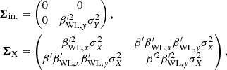
respectively.
Then, the posterior distribution is given by
 (A.10)
Here, p(θ) and p(ψ) are priors. We adopted a flat prior [ − 104, 104] to the normalization and a student’s t1 distribution with one degree of freedom on the slopes so that the slope angles become uniformly distributed. As for a noninformative prior distribution on the normalization of the variance of the parent distribution, a scaled inverse χ2 distribution as a conjugate prior, satisfying that posterior distributions have the same probability distribution family as the prior distribution.
Appendix B: WL mass calibrations
Cluster WL analysis extracts masses by an ensemble average of galaxy ellipticity which is composed of coherent WL signals synthesized to the intrinsic ellipticity. Thus, measurement accuracy depends on the number of background galaxies. For instance, there is no mass bias if an infinite number of background galaxies is available. In contrast, if the number of background galaxies was not sufficient, given the WL signal, each measured mass would be accidentally overestimated or underestimated. With the secure background selection using P(z) in the HSC-SSP Survey, the number density of background galaxies depends strongly on the cluster redshift (Figs. 2 and B.1), varying from ∼10 to 1 [arcmin−2] by changing the cluster redshift from 0.1 to 0.8. Even though we measure individual cluster masses, there might be bias and scatter in the measured WL masses.
We evaluated such systematics using a mock shape catalog, realizing our observing conditions. We assume a spherical NFW model and no lensing effect from the large-scale structure. Other effects (e.g., miscentering effect and halo triaxiality) as appeared in numerical simulations are not included. WL calibrations using numerical simulations are reported in the literature (e.g., Meneghetti et al. 2010; Becker & Kravtsov 2011; Giocoli et al. 2012; Umetsu et al. 2020; Euclid Collaboration: Giocoli et al. 2024). The quantitative details are not comparable due to differences in the redshift range, the mass range, the overdensities, the fitting method, the number of samples, and simulation types. However, the overall trend of the bias in the relationship between WL mass and true mass is negative by several per cent and approaches zero as the true mass increases. This could be explained mainly by the fact that the probability of the major axes of halo mass distributions aligning with the sky plane is higher than in the line-of-sight direction. Although our tests include minimal effects, we placed more emphasis on a catalog that represents the observational conditions and our analysis. To asses the bias and scatter in the WL mass measurement, the sufficient number of clusters in each mass and redshift bin is required, otherwise, an accidental over- or underestimation cannot be ruled out. The mock clusters are uniformly distributed in the logarithmic space of mass range of ![Mathematical equation: $ [0.8,30]h_{70}^{-1}10^{14}M_\odot $](/articles/aa/full_html/2025/08/aa53708-25/aa53708-25-eq228.gif) and in the linear space of the redshift range of [0.1, 1]. The concentration parameter uses Bhattacharya et al. (2013). The adopted number density of the background galaxies follows our result (bottom panel of Fig. B.1). We randomly pick up galaxies from the whole HSC catalog (Li et al. 2022; Nishizawa et al. 2020), used in our analysis by satisfying eq. (1) as background galaxies. The catalog contains the photometric redshift, its probability, and ellipticity. The spatial distributions of background galaxies are uniformly distributed, where we do not consider star mask effects. The intrinsic shape ellipticity is calculated by randomly rotating the catalog ellipticity. We then synthesize the lensing signal to the intrinsic ellipticity. We make 9000 mock clusters and then repeat the same tangential shear analysis.
and in the linear space of the redshift range of [0.1, 1]. The concentration parameter uses Bhattacharya et al. (2013). The adopted number density of the background galaxies follows our result (bottom panel of Fig. B.1). We randomly pick up galaxies from the whole HSC catalog (Li et al. 2022; Nishizawa et al. 2020), used in our analysis by satisfying eq. (1) as background galaxies. The catalog contains the photometric redshift, its probability, and ellipticity. The spatial distributions of background galaxies are uniformly distributed, where we do not consider star mask effects. The intrinsic shape ellipticity is calculated by randomly rotating the catalog ellipticity. We then synthesize the lensing signal to the intrinsic ellipticity. We make 9000 mock clusters and then repeat the same tangential shear analysis.
The upper panel of Fig. B.1 shows a measurable fraction in the z and M200 plane. For a visual purpose, we smoothed it with a Gaussian kernel with dz = 0.1 and  . We successfully measure cluster WL masses at z ≲ 0.4 and
  with more than 95%. In contrast, the higher the redshift and the lower the mass, the more difficult it is to measure WL masses. Therefore, our measured clusters selectively have a positive bias in the WL mass. The gray shadow region represents the z and
  distribution for our sample of the eRASS1 clusters, obtained by the scaling relation analysis (Sec. 3.4). The sample is distributed around ∼95% measurable fraction. Given the 75 association clusters, the number of the measurable clusters is ∼0.95 × 75 ∼ 71, which agrees with our case of the 72 clusters.
There are two proposed WL mass calibrations. First is to calibrate between  and
and  used in the scaling relations. The second is to calibrate the mass and concentration relation.
For the WL mass calibration of M500, we use the x parameters only. Figure B.2 shows the mass bias (black circles),  , for the mock clusters without the measurement errors and its average values (green boxes) in each mass and redshift bin. The measurable fraction (red solid lines) decreases as the mass is lower and the redshift is higher. In the region around the true mass where the measurable fraction is generally lower than 50%, the black points show a selective deviation from unity, and the average values exhibit positive biases. In contrast, the mass bias where the measurable fraction is more than ∼75% is close to unity. The mass dependence of the mass bias is likely to be non-linear. Thus, it is essential to reflect our mass distribution so that a linear equation can describe the WL mass calibration. We first performed the scaling relation analysis without the WL mass calibration and measured the parent population. We then excluded the mass range where the probability of the target clusters being present is less than 10−6. The magenta hatched boxes in the Fig. B.2 illustrate the excluded ranges for mass and redshift where the mass bias changes non-linearly. The resulting baseline parameters ( blue solid lines in Fig. B.2 ) are listed in Table B.1. There is no significant alteration in the results when we either apply the minimum threshold of 10−5 or choose a random 90% sample of the clusters.
For  and
and  , we select the clusters with the condition that the probability of the target clusters being present is larger than 10−6. The WL biases in M200 and c200 are correlated, as shown in Fig. C.1. We evaluated the WL mass calibration parameters by simultaneously fitting all the measurements with the covariance error matrix. The result is shown in Table B.1. Since the intrinsic WL scatter in the mass and concentration is highly coupled, the intrinsic WL scatter becomes large. In the regression analysis, we used the parameters of the WL mass calibration as priors, taking into account its error covariance matrix.
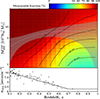 |
Fig. B.1. Top: Fraction of 9000 synthetic clusters for which WL masses can be measured in the |


WL mass calibrations for  ,
,  and
and  , where σWL = exp(lnσWL).
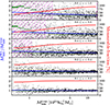 |
Fig. B.2. Mass bias, |

Appendix C: Mass-richness-CR relation with E(z)
Since the redshift dependence of the overdensity masses follows MΔ ∝ ρcr(z)rΔ3 ∝ E(z)−1 and the soft-band luminosity follows LX ∝ ρcr(z)2rΔ3 ∝ E(z), we here replace M500, CR, and λ by M500E(z), CRE(z)−1, and λE(z) in the scaling relation analysis, respectively. The result changes only the normalization in response to the replacement (the first column in Table C.1).
Scaling relation parameters using M500E(z), CRE(z)−1, and λE(z) or CAMIRA richness, N.
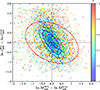 |
Fig. C.1. The points represent the logarithmic WL biases ( |
Appendix D: Mass-richness-CR relation with the CAMIRA richness
We cross-match the HSC CAMIRA clusters (Oguri et al. 2018, Oguri et al. in prep.) with the eRASS1 clusters. We used the internal CAMIRA catalog with the S21A version. The tolerances for the spatial and redshift differences are 4 arcmin and 0.1 in the crossmatching. The 68 clusters out of the 78 eRASS1 clusters are matched. In the scaling relation analysis, we replace the richness, λ, by the CAMIRA richness Ncamira. Since the masses of two clusters are not measurable, the number of clusters is 66 in the scaling relation analysis. The resulting parameters are described in the second column in Table C.1. The result changes little except for the redshift-dependent slope in the richness.
 |
Fig. D.1. The CAMIRA richness and mass scaling relation. The black circles denote the overlapped 66 clusters. The orange solid and magenta dotted lines are the best-fit scaling relations concerning the WL and true masses, respectively. The orange region is the 1σ uncertainty of the scaling relation with the WL masses. The blue solid line and region are the best-fit and 1σ uncertainty with the eRASS1 richness (Fig. 7), respectively. |
Appendix E: WL Mass table
Table E.1 presents the WL masses and concentrations of the eRASS1 clusters.
Cluster properties and their NFW weak-lensing parameters of  ,
,  , and
, and  .
.
All Tables
Scaling relation parameters using M500E(z), CRE(z)−1, and λE(z) or CAMIRA richness, N.
All Figures
|
Fig. 1. Left: Count-rate (CR) versus redshift (z). Right: Richness (λ) versus redshift (z). The dotted line is the threshold described by a function connecting two constants with a linear function. Colors in all the panels denote the S/N of the reduced tangential shear profile. The circles, diamonds, squares, and up-triangles denote the clusters with 1D WL analysis only, 1D and 2D WL analysis, non-WL analysis, and misassociation, respectively. |
| In the text | |
|
Fig. 2. Weak-lensing masses ( |
| In the text | |
|
Fig. 3. Mass map for the J141507.1-002905 and J141457.8-00205 field (30′×30′). The black contours represent the reconstructed WL mass map spaced in units of 1σ bootstrapping error. The diameter of the black circle in the lower left corner represents the Gaussian smoothing FWHM = 400 kpc in the mass reconstruction. Blacked-out areas are the masked regions of bright stars. The blue + and × are positions of J141507.1-002905 and J141457.8-00205, respectively. The system is MCXC J1415.2-0030 (Piffaretti et al. 2011). The blue and cyan contours are the eRASS1 and XMM-Newton X-ray contours (Miyaoka et al. 2018), respectively. An X-ray bright point source in the western component is removed in the XMM-Newton contours. It was properly identified when the eRASS1 cluster catalog was constructed. At the same time, diffuse X-ray emission in the XMM-Newton image appeared even after removing the X-ray point source thanks to a higher angular resolution. The system is composed of three components with S/N ∼ 6.7σ for J141457.8-00205, ∼4.7σ for J141507.1-002905, and ∼5.3σ for the western component. |
| In the text | |
|
Fig. 4. HSC images for misassociation clusters. Overlaid with white contours representing red galaxy distribution, stepped by two galaxies per each pixel above two galaxies. |
| In the text | |
|
Fig. 5. Stacked profiles for the three misassociation clusters (top), the 12 poor-fit clusters (middle), and the 63 other clusters (bottom). The y-axis represents r × ⟨Σ+⟩ (filled colors) or r × ⟨Σ×⟩ (open colors). The + components for the 63 other clusters and the 12 poor-fit clusters are higher than the × components, while both the + and × components for the 3 misassociation clusters are consistent with the null. |
| In the text | |
|
Fig. 6. Stacked tangential profiles for 3 subsamples divided by redshift ranges of 0.4 < z (red diamonds), 0.2 < z ≤ 0.4 (blue squares), and 0.1 < z ≤ 0.2 (magenta upward triangles), and the 12 poor-fit clusters (green downward triangles). The filled and open symbols denote positive and negative values, respectively. |
| In the text | |
|
Fig. 7. Scaling relations between the count-rate (left) the richness (right) and the WL ( |
| In the text | |
|
Fig. 8. WL mass and concentration relation at Δ = 200. The transparent gray banana regions represent the 1σ constraint on mass and halo concentration for the 72 association clusters. The orange and red shaded regions represent the 1σ constraints by stacked lensing analysis for the 53 clusters with single galaxy peaks and the 22 clusters with multiple galaxy peaks, respectively. The best-fit line and its 1σ uncertainty are shown as the blue solid line and region, respectively. The magenta line is the best-fit for the true mass and the true concentration. The brown, pink, red, and green lines are the results of numerical simulations of Bhattacharya et al. (2013), Child et al. (2018), Diemer & Joyce (2019), and Ishiyama et al. (2021), respectively. |
| In the text | |
|
Fig. 9. Redshift evolution for the mass-concentration relation. The best-fit line and its 1σ uncertainty are shown as the magenta solid line and region, respectively. The blue dotted lines are the results without the WL calibration. The brown and red dashed lines denote the normalizations of numerical simulations of Bhattacharya et al. (2013) and Diemer & Joyce (2019), respectively. |
| In the text | |
|
Fig. 10. Left: Best-fit distance from the eRASS1 centroids. The blue diamonds, green down-triangles, and magenta up-triangles represent the results of the spherical NFW model, the elliptical NFW model, and the inclusion of the multiple spherical NFW components, respectively. The red solid line, the light-blue dashed line, and the green dotted line are the best-fit for all the components, the inner Gaussian and the outer Gaussian, respectively. Right: Magenta up-triangles represent the distance from galaxy map peaks. The blue diamonds are the same as in the left panel. |
| In the text | |
|
Fig. 11. S/N of stacked mass maps for the subsamples (12′×12′). The black contours represent the reconstructed WL mass map spaced in units of 2σ bootstrapping error starting from 2σ. The first, second, and third rows from the top show the maps for the subsamples divided by richness, redshift, and the S/N in the tangential shear, respectively. These samples exclude the poor-fit and misassociation clusters. The left and right panels in the bottom row show the mass maps for the poor-fit and misassociation clusters, respectively. The selection criteria are described in the upper part of each panel. The white crosses denote the eRASS1 centroids. The white horizontal line corresponds to the smoothing FWHM of 1′. The number of clusters, the average redshift, and the average richness are described in the lower part of each panel. |
| In the text | |
|
Fig. 12. Stacked tangential shear profile for the 12 poor-fit clusters (same as Fig. 6). The green solid line denotes the best-fit model for a single NFW model, but showing |
| In the text | |
|
Fig. 13. Comparison of the baselines and the results of the poor-fit clusters. The green region and up-triangles are the results of the single NFW model for the 12 poor-fit clusters. The magenta region and squares are the results of the eRASS1 clusters considering the surrounding mass halos in the model fitting. The gray circles are the results of the total components, including the surrounding mass. The orange region and down-triangles are the results of the single NFW model for the six poor-fit clusters with a single galaxy peak. Left: Mass-concentration relation. Middle: Mass and the corrected CR relation. Right: Mass and richness relation. The lensing contribution from the surrounding halos cannot be ignored for the poor-fit clusters. Once we consider the surrounding halos, the concentration agrees with the baseline, but the masses expected from the count-rate or the richness are significantly overestimated. |
| In the text | |
|
Fig. 14. 2D halo ellipticity distribution. The solid line is the best-fit Gaussian distribution convolved with the average measurement error. |
| In the text | |
|
Fig. 15. Stacked mass maps for the 34 clusters analyzed with the elliptical NFW model. Top: Random orientations. Bottom: Aligned the major axis with the y-axis. The white dashed lines are auxiliary lines reflecting the median ellipticity. The white solid lines at the bottom right represent the 1 arcmin smoothing scale. |
| In the text | |
|
Fig. 16. Stacked eRASS1 (top) and galaxy (bottom) maps for the 34 clusters analyzed with the elliptical NFW model. The alignment is the same as Fig. 15. The white dashed lines are auxiliary lines reflecting the median ellipticity. The white solid lines at the bottom right represent the 1 arcmin smoothing scale. |
| In the text | |
|
Fig. 17. Offset distances between the WL centers and the eRASS1 centroids (red solid line), between the WL centers and the galaxy peaks (blue dashed line), and between the galaxy peaks and the eRASS1 centroids (green dotted line). It indicates that the offset directions of the galaxy peaks are different from those of the WL centers. |
| In the text | |
|
Fig. 18. Mass comparison with the Pz and CC selections. The blue solid line and the blue region are the best-fit and the 1σ uncertainty. |
| In the text | |
|
Fig. 19. Comparison with the literature. The blue solid line and the blue region are the best-fit and the 1σ uncertainty (Fig. 8), respectively. The magenta line is the true mass and concentration relation. The red and brown lines are the best-fit lines of Okabe & Smith (2016) and Umetsu et al. (2020), respectively, where the redshift zref = 0.3 of Umetsu et al. (2020) is converted to z = 0.21. The orange and red shaded regions represent the 1σ constraints by stacked lensing analysis for the 53 clusters with single galaxy peak, and the 22 clusters with multiple galaxy peaks, respectively. The green and pink shaded regions represent the 1σ constraints by stacked lensing analysis for the HSC-CAMIRA clusters (Okabe et al. 2019) with single galaxy peak and multiple galaxy peaks, respectively. The pink square, up-triangle and down-triangle are the results of stacked lensing analyses of Umetsu et al. (2016), Cibirka et al. (2017) and Sereno et al. (2017), respectively. |
| In the text | |
|
Fig. 20. Top: Mass comparison between |
| In the text | |
|
Fig. B.1. Top: Fraction of 9000 synthetic clusters for which WL masses can be measured in the |
| In the text | |
|
Fig. B.2. Mass bias, |
| In the text | |
|
Fig. C.1. The points represent the logarithmic WL biases ( |
| In the text | |
|
Fig. D.1. The CAMIRA richness and mass scaling relation. The black circles denote the overlapped 66 clusters. The orange solid and magenta dotted lines are the best-fit scaling relations concerning the WL and true masses, respectively. The orange region is the 1σ uncertainty of the scaling relation with the WL masses. The blue solid line and region are the best-fit and 1σ uncertainty with the eRASS1 richness (Fig. 7), respectively. |
| In the text | |
Current usage metrics show cumulative count of Article Views (full-text article views including HTML views, PDF and ePub downloads, according to the available data) and Abstracts Views on Vision4Press platform.
Data correspond to usage on the plateform after 2015. The current usage metrics is available 48-96 hours after online publication and is updated daily on week days.
Initial download of the metrics may take a while.