| Issue |
A&A
Volume 703, November 2025
|
|
|---|---|---|
| Article Number | A193 | |
| Number of page(s) | 16 | |
| Section | Galactic structure, stellar clusters and populations | |
| DOI | https://doi.org/10.1051/0004-6361/202554967 | |
| Published online | 18 November 2025 | |
Internal dynamics and structure of Cepheus OB4
The asymmetric expansion of Berkeley 59
1
Fakultät für Physik und Erdsystemwissenschaften, Universität Leipzig,
Linnéstraße 5,
04103
Leipzig,
Germany
2
Departamento de Física, Faculdade de Ciências, Universidade de Lisboa,
Edifício C8, Campo Grande,
1749-016
Lisbon,
Portugal
3
Instituto de Astrofísica e Ciências do Espaço, Faculdade de Ciências, Universidade de Lisboa,
Ed. C8, Campo Grande,
1749-016
Lisbon,
Portugal
4
Istituto Nazionale di Astrofisica (INAF) – Osservatorio Astronomico di Palermo,
Piazza del Parlamento 1,
90134
Palermo,
Italy
★ Corresponding author: This email address is being protected from spambots. You need JavaScript enabled to view it.
Received:
1
April
2025
Accepted:
18
September
2025
Abstract
Context. Accurate measurements of the internal dynamics of young stellar clusters can be used to extract crucial information about their formation process. With Gaia, we are now able to trace stellar motions and study the dynamics of star clusters with unprecedented precision. A fundamental requirement for this analysis is a well-defined and reliable list of probable members.
Aims. We examined a region with a radius of 2° in Cepheus OB4, centered on the young cluster Berkeley 59, to build a reliable candidate member list. Our catalog enables the determination of structural and kinematic parameters of the cluster and other properties of its stellar population.
Methods. We compiled a catalog of optical and near-infrared photometry, along with precise positions and proper motions from Gaia DR3, for sources in the Cepheus OB4 field. The membership probabilities were determined using a probabilistic random forest algorithm and were further refined by requiring positions in the Hertzsprung-Russel diagram consistent with a young age. Based on a list of 1030 probable members, we estimate that the distance to Berkeley 59 is 1009 ± 12 pc. Masses, extinction, and ages were derived by fitting the spectral energy distributions to atmospheric and evolutionary models, and internal dynamics was analyzed using proper motions relative to the mean motion of the cluster.
Results. Berkeley 59 exhibits an asymmetric expansion pattern. The velocity increases outward, and the preferred motion is toward the north. The initial mass function between 0.4 and 7 M⊙ follows a single power law (dN/dM ∝ M−α) with a slope α = 2.3 ± 0.3, which is consistent with Salpeter’s slope and previous studies in the region. We estimated the median age of the region based on the Hertzsprung-Russel diagram as 2.9 Myr. The velocity dispersion of Berkeley 59 exceeds the virial velocity dispersion derived from its total mass (650 ± 30 M⊙) and half-mass radius (1.71 ± 0.13 pc). The two-dimensional motions of a stellar group located ~1° north of Berkeley 59 provide further support for the previously proposed scenario of triggered star formation.
Key words: stars: kinematics and dynamics / stars: pre-main sequence / open clusters and associations: individual: Berkeley 59 / open clusters and associations: individual: Cepheus OB4
© The Authors 2025
 Open Access article, published by EDP Sciences, under the terms of the Creative Commons Attribution License (https://creativecommons.org/licenses/by/4.0), which permits unrestricted use, distribution, and reproduction in any medium, provided the original work is properly cited.
This article is published in open access under the Subscribe to Open model. This email address is being protected from spambots. You need JavaScript enabled to view it. to support open access publication.
1 Introduction
Stars predominantly form in clusters and associations and emerge within giant molecular clouds through fragmentation and gravitational collapse (Lada & Lada 2003; Gutermuth et al. 2009; Wright 2020). These young stellar groups often retain the turbulent and substructured nature of their parent clouds, which might reflect large-scale dynamical processes (Tan 2000; Inutsuka et al. 2015; Sills et al. 2018). The subsequent evolution may be strongly affected by the formation of massive stars that expel the surrounding gas through intense radiation and stellar winds, thus reducing the gravitational binding of the system (Goodwin & Bastian 2006). The extent to which embedded clusters and their substructures survive this phase and merge into bound stellar systems remains an open question, but kinematic signatures of expansion can provide key evidence of ongoing dispersal (Parker et al. 2014; Sills et al. 2018; Armstrong & Tan 2024).
One of the primary challenges in studying the early phases of star cluster formation has been to obtain precise kinematic xmeasurements of young stars. The data from the Gaia space mission (Gaia Collaboration 2016) have revolutionized our ability to trace stellar motions and study the dynamics of star clusters with unprecedented precision (e.g. Kuhn et al. 2019; Cantat-Gaudin et al. 2019; Meingast et al. 2021). In particular, expansion has been reported for a number of young clusters (Pang et al. 2021; Guilherme-Garcia et al. 2023; Della Croce et al. 2024), star-forming regions, and OB associations (Zari et al. 2019; Armstrong et al. 2022). The analysis of Della Croce et al. (2024) revealed that a significant fraction of clusters younger than 30 Myr appears to be expanding, while the older clusters are mostly consistent with an equilibrium configuration. Most of these studies did not include very young populations (a few million years), however, which is crucial for investigating the kinematic patterns linked to the early dynamical evolution of these systems. The younger clusters and star-forming regions are affected by (often differential) reddening, which complicates the membership determination and typically requires a more individual approach. Kuhn et al. (2019) reported that 75% of the 28 clusters that were younger than 5 Myr showed expansion, and those that are still embedded in molecular clouds were less likely to expand than those that were partially or fully revealed. Additionally, the authors found no evidence of subgroup or multiple cluster mergers, which suggests that if hierarchical cluster assembly occurs, it must take place quickly during the embedded phase. In λ Ori, Armstrong & Tan (2024) reported evidence of a significant substructure, but this is preferentially located away from the central cluster core, which is smooth and likely remains bound. They reported strong evidence for expansion, which also appears asymmetric. The highest expansion rate was directed nearly parallel to the Galactic plane. In their 3D kinematic study of 18 star clusters and associations, Wright et al. (2019) and Wright et al. (2024) reported that the vast majority (~95%) of groups show expansion, also predominantly asymmetrically. These findings challenge the simple residual gas expulsion models that predict a radial expansion pattern. On the other hand, the observed expansion in NGC 2244 (Lim et al. 2021; Mužić et al. 2022) appears to be radially symmetric.
We concentrate on the Cepheus OB4 region (Kun et al. 2008; Rossano et al. 1983), which is dominated by the central cluster Berkeley 59. The age of the cluster is ~2 Myr (Pandey et al. 2008; Majaess et al. 2008), and its distance is ~1.1 kpc (Kuhn et al. 2019). The cluster hosts several OB stars in its core (Skiff 2014), and it is situated within the surrounding H II region Sharpless 171 (S 171). S 171 is expanding through interaction with hot stars of Berkeley 59 (Gahm et al. 2022). To the north of Berkeley 59 lies the nebula NGC 7822, which is also labeled as bright-rimmed cloud 2 (BRC2) by Sugitani et al. (1991), which is an integral part of S 171. Previous studies investigated the cluster at optical bands (Pandey et al. 2008; Eswaraiah et al. 2012; Panwar et al. 2018) and by X-ray and in the near- and mid-infrared (Koenig et al. 2012; Rosvick & Majaess 2013; Getman et al. 2017; Mintz et al. 2021). Kuhn et al. (2019) combined these methods with astrometric data from Gaia; the results relative to the expansion (or contraction) state of the cluster remain ambiguous because the uncertainties are large. Recently, Panwar et al. (2024) presented the first substellar initial mass function (IMF) in Berkeley 59. We performed a new membership analysis of Cepheus OB4 using the supervised machine-learning algorithm called probabilistic random forest (PRF; Reis et al. 2019). The same method was tested before on the Rosette Nebula (Mužić et al. 2022), which doubled the number of known members of the region and allowed us to detect a clear expansion pattern of the central cluster NGC 2244 and the motions of other groups in its vicinity.
This paper is structured as follows. In Section 2, we present the details of the dataset we used, including the photometric and astrometric catalogs. The primary membership selection method using the PRF algorithm is given in Section 3, followed by the additional constraints on the membership in Section 4. We present the analysis of spatial and kinematic properties of the selected members (Section 5). Section 6 focuses on the properties of Berkeley 59, including its mass function, and we discuss its dynamical state. Finally, Section 7 summarizes the work and lists the main conclusions.
2 Dataset
2.1 Catalog assembly
The primary catalog was based on Gaia DR3 (Gaia Collaboration 2016, 2023), which offers high-precision astrometric data along with optical photometry. A cone search with a radius of 2° about the center of Berkeley 59, (α, δ)=(00: 02 : 16.8, +67 : 26 : 28), as resolved by SIMBAD (Wenger et al. 2000), yields about half a million sources. We used a radius of 2° to include other structures of the Cepheus OB4 association that may be related to Berkeley 59 (Mintz et al. 2021). Additional optical and near-infrared photometry was queried from 2MASS (Skrutskie et al. 2006) and Pan-STARRS data (Flewelling 2017) in the same region on the sky. The catalogs were then cleaned to ensure that only high-quality measurements were included. For the Gaia data, we only accepted sources with a valid proper motion measurement. The 2MASS data were restricted by using the ph_qual flag, for which only values A, B, or C were allowed. These quality flags ensure that the detection of a source is above a certain sensitivity level1. In the Pan-STARRS data, we disregarded any measurements with quality flags 1, 2, 64, and 1282. The three catalogs were then joined in TopCat (Taylor 2005) using Gaia DR3 as the base catalog: We kept all the sources from Gaia and added information from the other two catalogs. This means that all the sources in the final catalog have proper motions, but may not have measurements in a complete set of photometric filters. This is an important point to consider when applying machine-learning techniques, as we discuss below. The matching radius used in TopCat was 1″. The resulting catalog of the region after filtering contains 443 212 sources.
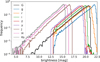 |
Fig. 1 Density of sources in our final catalog as a function of magnitude. |
Photometric completeness intervals.
2.2 Catalog completeness
The completeness limit of each photometric band was defined as the magnitude at which the density of the sources reached maximum (Fig. 1). In Table 1 we present the completeness intervals. The faint end is equivalent to masses between 0.1 and 0.6 M⊙, depending on the filter, for an age of 2 Myr, a distance of ~1000 pc, and an average extinction of AV=4 mag (Panwar et al. 2018), according to the BHAC15 models (Baraffe et al. 2015). The shallowest filter (in terms of mass; Pan-STARRS g) was not used in the final run of the selection, and our results are therefore limited by the Gaia G and Pan-STARRS r bands, that is, by about 0.4 M⊙. We adopted this limit for the analysis below.
3 Membership determination using the probabilistic random forest classifier
In this section, we describe the method for membership determination using the PRF algorithm. In Section 3.1, we describe the training set in detail, and in Section 3.2 we present details of the model construction and its evaluation.
3.1 Construction of the training set
Our classification problem has two classes: members of the cluster, and other sources, which we call nonmembers. Thus, the training set consisted of the lists of probable members and non-members, which were combined to form the final training set. In the following, we describe the creation of these two lists. This step is critical because the quality of the model is defined by the quality of the training set in supervised machine-learning problems.
3.1.1 Member list
To construct a high-probability member list, we combined the member catalogs from Getman et al. (2017), Mintz et al. (2021), and Panwar et al. (2018). The selection in the first two catalogs was performed based on the X-ray and/or mid-infrared properties of the sources, and the third catalog used optical color-magnitude diagrams for the selection. We limited our selection of members to sources within 30′ of the center, where the concentration of sources belonging to Berkeley 59 is highest. After cross-matching the list of previously reported members with our catalog, we had 860 common sources in this area.
Next, we applied a cut to this member list based on the proper motions of the stars. Fig. 2 shows the proper motions of the sources in a field of 30′ around Berkeley 59, along with the probable members from the literature. The mean proper motion (3σ clipped) of the members from the literature is μα cos δ = −1.62 ± 0.59 mas yr−1 and μδ = −1.79 ± 0.69 mas yr−1. The semimajor axes of the orange ellipse are equivalent to 1.2σ in α and δ and are centered on the mean proper motion. The 500 sources inside this ellipse were retained in the training set. The extent of the ellipse is somewhat arbitrary and was chosen with the intention to be conservative rather than complete.
This list can be further refined by using the position of the stars in a color-magnitude-diagram (CMD; Fig. 3). Young stars are expected to have redder colors and therefore to appear to the right of the main bulk of stars. The three colors we used were determined visually by comparing various diagrams in TopCat (Taylor 2005) and observing which separated the members (redder colors) and nonmembers (bluer colors) best. The dashed lines mark our selection criteria, roughly aided by the shape of the 2 Myr PARSEC isochrone (Bressan et al. 2012; Pastorelli et al. 2020) shifted to a distance of 1100 pc. The sources located to the right of the lines marking the selection criteria in all three CMDs were retained in the member training sample. Stars that lacked some of the photometric points were retained if they passed the cuts in the remaining diagrams. This cut reduced the member list to 468 sources.
A final cut was applied using parallaxes. We rejected any source that was located at a distance that differed from the cluster distance using the parallax measurement of Gaia. All sources with a score ![Mathematical equation: $\[\zeta=|\varpi-\bar{\varpi}| / \sqrt{\sigma_{\varpi}^{2}+\sigma^{2}}>3\]$](/articles/aa/full_html/2025/11/aa54967-25/aa54967-25-eq1.png) were removed from the member list, where ϖ and σϖ represent the parallax measurement and uncertainty for each star, and
were removed from the member list, where ϖ and σϖ represent the parallax measurement and uncertainty for each star, and ![Mathematical equation: $\[\bar{\varpi}\]$](/articles/aa/full_html/2025/11/aa54967-25/aa54967-25-eq2.png) and σ are the weighted mean and standard deviation of the entire sample, correspondingly. The 6 excluded sources are marked with red crosses in Fig. 4. This left 462 probable member sources for the final training set.
and σ are the weighted mean and standard deviation of the entire sample, correspondingly. The 6 excluded sources are marked with red crosses in Fig. 4. This left 462 probable member sources for the final training set.
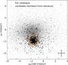 |
Fig. 2 Gaia DR3 proper motions of objects in Cepheus OB4 (gray dots). The black dots represent the 860 candidate members from the literature within a radius of 30′ from the center of Berkeley 59. The orange ellipse indicates the proper motion selection criterion for constructing the member training set. In the lower right corner, we show the mean proper motion uncertainty. |
3.1.2 Nonmember list
The nonmember list was sampled from the annulus with an inner radius of 1° and an outer radius of 2° from the center. This region was selected to avoid the densest part of Berkeley 59, and thus, to minimize the inclusion of potential members while staying close enough to sample similar extinction properties. We used two criteria to construct the nonmembers lists: (1) sources whose individual proper motion did not intersect the orange ellipse in Fig. 2 within 1σ; and (2) blue sources located to the left of the dashed selection lines shown in Fig. 3. The final nonmember list obtained by this procedure contained 282 714 unique sources.
3.2 Training and evaluation of the model
In this section, we describe the parameters we used to construct the model (Section 3.2.1). Next, we proceed with the evaluation of the model and a comparison between different runs (Section 3.2.2).
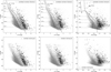 |
Fig. 3 Color–magnitude diagrams we used to select the training set. The black dots in the top panels show candidate members from the literature, and the gray dots mark all the sources in the field. The dashed lines show the selection criteria, and the solid lines represent the 2 Myr PARSEC isochrones, shifted to a distance of 1100 pc (Kuhn et al. 2019). In the lower panels, the black dots represent the probable members we selected for the training set after the proper motion, color, and parallax filters. |
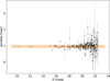 |
Fig. 4 Parallax measurements for the candidates of the member training set, selected based on proper motions and colors (black dots). The dotted orange line represents the weighted average of the parallaxes, and the shaded area marks the ±1σ range. The red crosses mark the sources that were excluded from the final member training set (see text for the details of the criterion we applied). |
3.2.1 Characteristics of the PRF
There are several important points to discuss before an PRF model is constructed. They are listed below. During the construction of the training set, we saw that the main distinguishing features are their proper motions, their positions in CMDs, and the parallax measurements. Therefore, the main features that we used were the proper motions, parallaxes, magnitudes, and colors constructed from the differences of magnitude pairs. In total, there were 39 available features. Generally speaking, it is desirable to select features in order to reduce the computation time and to potentially improve the performance of the model by avoiding overfitting. To this end, we used the recursive feature-elimination procedure, in which an initial run of the model (as described in Section 3.2.2) was performed to extract the feature importance. Next, the model was run again after the least relevant feature was removed, and it was run again after the two least relevant features were removed. This was repeated until the lowest number of features was reached, which we set to 5. At each step, the training set was split ten times in the same way as described in Section 3.2.2. From this, we calculated an average performance metric in the form of Matthews correlation coefficient (Matthews 1975). The performance of the model steeply increased until it reached maximum at 16 features. After this, it continued to decrease slightly, with some oscillations. We therefore kept the 16 most important features, to which we added the J − KS color. This color was specifically included because the infrared data at the bright end are very important, where the optical filters are largely saturated. The number of objects in this region is significantly smaller than at the faint end, and infrared colors are therefore deemed less important by the model. After inspecting the resulting infrared CMDs, we decided to add this feature manually, however.
The PRF algorithm contains various adjustable hyperparameters, but their effect on the results is found to be insignificant. To assess this, we altered individual parameters while maintaining others unchanged at their default settings. We varied the parameter n_estimators (number of trees) from 1 to 1000, max_depth (representing the depth of each tree in the forest) from 1 to 50, and max_features (maximum number of features considered at each node split) from 3 to 17 (all possible features). The accuracies varied by no more than 1% from the mean value in the tested range. As a result, we chose to adopt the default parameter values (n_estimators=100, max_depth=10, max_features= ![Mathematical equation: $\[\sqrt{N}\]$](/articles/aa/full_html/2025/11/aa54967-25/aa54967-25-eq3.png) , where N=17 is the total number of available features).
, where N=17 is the total number of available features).
While it is a requirement for all objects in our catalog to possess proper motion measurements, some of them lacked one or more photometric measurements. A notable advantage of the PRF algorithm lies in its ability to handle missing data without requiring any specific treatment of the data because feature measurements are represented as PDFs. During the training and prediction stages, we assigned an object with a missing value for a particular feature a probability of 0.5 to propagate to either the member or nonmember tree nodes.
To create the training set, we combined the member list, consisting of 462 sources, with the nonmember catalog, containing 282 714 sources. To compensate for this imbalance, we resampled the two classes by either oversampling the member class, undersampling the nonmember class, or a mixture of both. For this task, we used the Python package imbalanced-learn (Lemaitre et al. 2016). The sampling_strategy keyword was used to control the extent of random over- or undersampling. For instance, setting sampling_strategy=0.5 resulted in either under-sampling the majority class or oversampling the minority class such that we obtained a ratio of 1:2 between minority and majority class. The combinations we used are detailed in Table A.1. We selected the sampling parameters so that a reasonably balanced training set was assembled, that is, we kept the numbers in the same order of magnitude.
3.2.2 Evaluation and comparison of PRF runs
The PRF was run six times (runs A to F in Table A.1) with different sampling strategies and the same default hyperparameters. We evaluated the performance of these runs using a cross-validation. The main training data were split into a set of test and train data with a ratio of 1:4, and we used stratified sampling in order to preserve the ratio of the two classes. For each classifier, 50 test and train split samples were created randomly, and the PRF was rerun for each of them.
We used four different metrics to compare the outcome of the various runs. These were the F1 score, the area below the receiver operating characteristic curve (ROC_AUC), the area below the precision recall curve (PR_AUC), and the Matthews correlation coefficient. The results are given in Table A.1 and are shown in Fig. A.1. The error bars were calculated as the standard deviation of the resulting scores from 50 random split samples.
Fig. A.1 shows that run C (the run with the smallest training set) performed worst in all four metrics. The remaining five runs performed similarly well (above 99% in all metrics). We maintained these five runs and used them to classify the full catalog. Each run assigned a certain membership probability to each source: The final probability was calculated as the arithmetic mean of the five values.
In Fig. A.2, we show the relative feature importance for the 17 features in run F. The distribution looks similar for the other runs. The proper motion in Dec is by far the most significant feature because the proper motion of the cluster differs most in this direction from the field population. Next follow two optical-NIR colors, then the proper motion in RA, and parallax is in fifth place. The proper motion of the cluster in the RA direction is relatively similar to the field motion, and this feature is therefore slightly less informative than proper motion in Dec. The strong performance of the classifier is primarily due to the careful construction of the training set, where we applied informed cuts in proper motion, colors, and parallax (Figs. 2, 3, 4), which allowed us to clearly separate the classes. Moreover, the deliberate selection of the 17 most informative features further enhanced the performance.
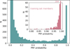 |
Fig. 5 Distribution of the membership probability of the final catalog limited to objects 30′ from the center for clarity. The four leftmost columns are capped for better readability. The inset diagram shows the prediction for all objects labeled as members in the training set. The rightmost column of the inset diagram is capped, and its value is depicted next to it. |
4 Further constraints on the membership
4.1 High-probability candidates from the PRF
The outcome of the procedure described in the previous section was a membership probability for each source. The green histogram in Fig. 5 shows a distribution of these probabilities for the inner 30′ from the cluster center (the limit was set for plotting clarity), while the inset diagram shows the prediction for all the objects that were identified as members in the training set. We recovered 454 out of 462 (98%) with a probability higher than 90%, and all of them with a probability higher than 79%. Considering the high recovery rate and with the aim of a cleaner classification, we considered objects with a probability ≥90% to be members of the region. This resulted in a total number of 1224 candidate members. In the following, we further refine this selection.
To estimate the contamination rate in our sample, we applied the same PRF classifier as described in Section 3.2.2 to a nearby control field that was not related to Berkeley 59 and centered at (α, δ)=(23:44:20.5, +71:10:07), with a radius of 1°. The catalog for this control field was constructed using the same procedure as outlined in Section 2.1, and it contained ~127 000 objects. None of these objects was classified as a member with a probability higher than 80%, and only 47 (~0.04%) were assigned a probability of 50% or higher. These findings suggest that the contamination rate in our sample is likely to be very low.
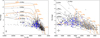 |
Fig. 6 Hertzsprung-Russell diagram showing the candidates with membership probabilities ≥90% (black dots). The blue crosses mark candidates located in the southern filaments (see Sect. 4.3). The isochrones (solid gray lines) and the lines of constant mass (dashed orange lines) are from the PARSEC series (Bressan et al. 2012; Pastorelli et al. 2020). A typical error bar is shown in the lower left corner. Objects located below the 30 Myr isochrone are considered contaminants. The right panel is the zoomed-in version of the left panel. |
4.2 SED fitting and HR diagram
Using the optical and infrared photometry, we constructed spectral energy distributions (SED) for the PRF-selected candidate members and used the stellar synthetic atmosphere models to derive the effective temperature (Teff), extinction (AV), and surface gravity (log(g)). For objects with excess emission in WISE photometry, we fit the SED based only the optical and near-infrared portions of the spectrum. Otherwise, the full available wavelength range was included in the fit. The metallicity was set to the solar value. We used BT-Settl models (Allard et al. 2011) and explored a Teff between 2000 K and 20 000 K in 100 K increments. The AV was varied between 0 and 10 mag in steps of 0.25 mag, and log(g) between 3.5 and 5.0, which is appropriate for young low-mass stars as well as field stars3. To obtain the best-fitting model, we performed a least-squares minimization using the square of the photometric uncertainties as weights. Before this, we modified the uncertainties to 5% of the flux value when the catalog values were lower than this. Otherwise, we noted a systematic bias in the majority of our fits, where the best-fit model provided a consistently poor fit to the infrared photometry. The model SEDs were scaled to match the median object fluxes.
In Fig. 6, we show the Hertzsprung-Russell (HR) diagram constructed using the Teff and AV derived from the SED fitting, assuming a distance of 1009 pc. The majority of the PRF-selected objects appear consistent with young ages, which validates our selection method. A group of sources is located below the 30 Myr isochrone, however, and the sources are likely background contaminants. These sources are all at the faint end of the apparent magnitude distribution (G ≳ 19) and have large parallax errors (mean ϖ/σϖ ~ 2, compared to ~9 for the full sample shown in the HRD). These sources comprise 10% of the PRF-selected member candidates and were removed from the further analysis. At this stage, we had 1106-member candidates.
4.3 Spatial distribution and distances
In Fig. 7. we show the high-probability candidate members from the PRF with ages younger than 30 Myr (black dots and blue crosses) overlaid on a Planck 857 GHz image (Planck Collaboration 2016). A zoomed-in version of the plot is shown in the right panel overlaid on an image from the Digitized Sky Survey (DSS4). The region is dominated by the central cluster Berkeley 59. At the northern edge of the left panel in Fig. 7, a small concentration of sources lies at the border of the HII region. It was previously called cluster 0 by Mintz et al. (2021) and BRC2 by Sugitani et al. (1991); Ogura et al. (2002) and was associated with the nebula NGC 7822 (Lozinskaya et al. 1987). Outside the Berkeley 59 region, we find sources in regions associated with the higher dust concentration. In the lower half of the left panel, the sources follow the filamentary structure of the molecular cloud.
The distance to the cluster was recalculated using the Gaia DR3 parallax measurements and applying the maximum-likelihood procedure following Mužić et al. (2019) and Cantat-Gaudin et al. (2018). Furthermore, Gaia parallaxes were shown to contain a bias that was discovered and characterized via quasar measurements. This bias depends in a nontrivial way on the position, color, and magnitude (Lindegren et al. 2021). To estimate the value of the parallax bias, we used the Python package5 based on the prescription given by Lindegren et al. (2021). The bias was removed from all the sources for which it could be calculated (~65% of the high-probability sources).
The distances are given in Table 2. The first row quotes the distance obtained using all the high-probability sources. We also calculated the distance to different subregions of our field of view, including the cluster Berkeley 59 (centered at (α, δ)=(00:02:16.0, +67:24:52) and within a radius of 18′; see Section 5.1), the clump in the northern part (cluster 0 in Mintz et al. 2021), and to the sources associated with the two dust filaments to the south of Berkeley 59. While the northern clump appears to be at a similar distance as the cluster, the sources associated with the southern dust filaments seem to be farther away by more than 700 pc. Although their proper motions and colors are similar to those of the other cluster members, their parallaxes agree significantly less well. Notably, the mean ϖ/σϖ for these sources is 2.4, indicating that their large parallax uncertainties allowed them to be classified as high-probability members. Interestingly, if we were to apply a distance modulus corresponding to 1800 pc, the southern sources would shift upward by 1.3 mag in the HR diagram, placing them in the 0.1–5 Myr region. This suggests that while these sources are likely genuinely young, they are situated well beyond the region of Berkeley 59. We excluded the 76 sources in the southern filaments (δ < 66.8°; blue crosses in Fig. 7) from the further analysis of this paper because they are probably located well behind Berkeley 59 and are not associated with it. We also recalculated the distance to the region (second row in Table 2).
The distance to Berkeley 59 we obtained is slightly shorter than 1100 ± 50 pc from Kuhn et al. (2019) and ~1.1 kpc from Gahm et al. (2022), and it agrees with 1.00 ± 0.06 kpc found by Panwar et al. (2024). For the remainder of this paper, we adopt the bias-corrected distance of Berkeley 59 of 1009 pc.
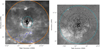 |
Fig. 7 Sources with membership probabilities ≥90% and consistent with ages <30 Myr (black dots) overplotted on the Planck 857 GHz image (left) and DSS red image (right) of the region around Berkeley 56. The sources that are likely located in the background, associated with the southern filaments, are marked with blue crosses. The solid orange circle encompasses the entire region (r=2°), the dashed blue circle shows the region in which the training sample was selected (r=30′), and the dotted black circle shows an extent of the cluster as derived from the radial profile (r=18′). The white star shows the position of the center of Berkeley 59 derived in Section 5.1. |
Distances to various structures in the region.
Selected members along with the Teff and AV from the SED fitting.
4.4 Summary of the member selection
We summarize the remaining sources in the final sample after applying various member selection cuts below.
Sources with the PRF probability ≥90%: 1224;
after removing objects below the 30 Myr isochrone: 1106;
after removing objects in the south (δ < 66.8°): 1030.
The following analysis was based on these final 1030 member candidates, which are listed in Table 3.
5 Spatial and kinematic properties of the candidate members
5.1 Center and radial distribution of Berkeley 59
We estimated the stellar surface density distribution of the cluster using a two-dimensional Gaussian kernel density estimator (KDE). The point of maximum density was taken as the center of the cluster, which is located at (α, δ)=(00:02:16.0, +67:24:52). The field was then divided into concentric annuli around the central point, and the radial profile (Fig. 8) was derived by counting the stars inside each annulus and dividing by the respective area. At a radius of about 18′, the density distribution decreases sharply, which we took as an indication that the outer radius of the cluster was reached. This radius corresponds to ~5.3 pc at the distance of Berkeley 59.
Limiting the extent of the cluster to r = 18′, we fit the radial distribution by a generalized radial profile known as the Elson-Fall-Freeman (EFF; Elson et al. 1987) in the following form:
![Mathematical equation: $\[\Sigma(r)=\Sigma_0\left[1+\left(\frac{r}{a}\right)^2\right]^{-\gamma / 2},\]$](/articles/aa/full_html/2025/11/aa54967-25/aa54967-25-eq4.png) (1)
(1)
where r stands for the projected distance from the center of the cluster, Σ0 is the central surface density, and a is a scale parameter. The core radius rc of the King profile (King 1966) is then given by
![Mathematical equation: $\[r_c=a\left(2^{2 / \gamma}-1\right)^{1 / 2}.\]$](/articles/aa/full_html/2025/11/aa54967-25/aa54967-25-eq5.png) (2)
(2)
The parameters of the best-fit profile (orange line in Fig. 8) are Σ0 = 14.0 ± 1.9 stars arcmin−2, a = 1.62 ± 0.23′, and γ = 1.83 ± 0.09. With this, we obtained the core radius rc = 1.72 ± 0.25′ = 0.50 ± 0.07 pc, depicted as the dashed gray line in Fig. 8. The core radius agrees with the radius derived by Pandey et al. (2008), which ranges between 1′ and 1.9′, depending on the selection of the sources included in the calculation. The slope γ is close to that of a modified Hubble model (γ=2; Binney & Tremaine 2008) and is similar to that of several other young clusters (Portegies Zwart et al. 2010; Kuhn et al. 2014, 2017; Miret-Roig et al. 2019). The mean surface density of the cluster, Σmean, is ~3.0 stars arcmin−2, which is equivalent to 35 stars pc−2 at a distance of 1009 pc.
In Table 4 we summarize various physical parameters of Berkeley 59, including those derived in this section.
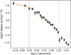 |
Fig. 8 Radial profile of Berkeley 59 in logarithmic scale. Each black dot shows the surface density of its corresponding annulus about the center. The dashed orange line is the best-fit EFF profile (Elson et al. 1987) up to a radius of 30′ (dotted gray line). The vertical dashed line represents the core radius derived from the profile fitting, and the dotted line marks the approximate outer radius of the cluster (r=18′). |
Summary of various kinematic and structural parameters of Berkeley 59.
5.2 Internal kinematics
To study the internal kinematics of the region, we started by calculating the error-weighted mean proper motion of Berkeley 59 within a radius of 18′. The mean proper motion was then subtracted from all individual sources in the region. Next, we corrected for the effect of perspective expansion (or contraction), which is caused by the projection of the radial cluster velocity onto the proper motion depending on the position of a star relative to the projection center (van Leeuwen 2009; Gaia Collaboration 2018; Kuhn et al. 2019). The radial velocity we used was vr = −13 km s−1, calculated as the weighted average of the numbers from Conrad et al. (2017) and Kharchenko et al. (2007), who gave RV = −14.9 ± 10.7 kms−1 and −12.5 ± 7.0 kms−1, respectively. As the center, we used the position calculated in Section 5.1. The effect of perspective expansion is weak on average (~0.02 mas yr−1), and it is more pronounced at the edges of the studied region (~0.15 mas yr−1).
5.2.1 Relative proper motions on the sky
In Fig. 9, we show the relative proper motion of high-probability members. In this plot, we show the central part of the studied region. A color-coded bar extends from each star to show the direction of its internal proper motion. There is no clear circular outward expansion pattern, which would reveal itself by resembling the color distribution similar to the disk shown in the lower right corner (see, e.g., Fig. 12 in Mužić et al. 2022). North of the center, however, predominant orange-reddish hues indicating motion in the northeast direction, while to the south of the cluster center lie more blue-shaded lines that signal a southwest motion. This indicates some level of expansion, roughly along the declination axis. To investigate this effect further, we introduced another color scheme that helps visualize expansion or contraction. To this end, we calculated the angle Φ, which is defined as the angle between the relative stellar proper motion and the line connecting the star to the cluster center. Φ = 0° translates into the proper motion vector that points away from the center, and Φ = 180° toward it. Fig. 10 shows the same region on the sky as Fig. 9, but the proper motion vector is color-coded according to the value of Φ. Purple hues indicate an outward motion from the center, and green hues indicate an inward motion toward the center. In this representation of the proper motions, the asymmetric expansion is seen more clearly, and it agrees with the interpretation of Fig. 9. Wright et al. (2024) examined the 3D dynamics of 18 star clusters and OB associations and found that the majority of the expanding groups expand asymmetrically. They suggested that in the absence of external forces that affect the stellar motion, this asymmetry likely arises from nonspherical initial conditions or anisotropic velocity dispersions prior to expansion.
In Fig. B.2, we zoom into the pillar to the north of the main cluster (cluster 0 in Mintz et al. (2021). As we showed in Section 4.3, the sources in this clump share a distance with Berkeley 59. The sources in the clump predominantly move away from the cluster. Moreover, Mintz et al. (2021) reported that cluster 0 contains a higher proportion of Class I than Class II sources than the central cluster Berkeley 59. These two findings speaks in favor of the scenario of triggered star formation that was previously suggested by Mintz et al. (2021). Inspecting the number ratio of Class I and Class II sources as a function of the distance from Berkeley 59 center, Mintz et al. (2021) reported that the ratio remains roughly constant out to ~1° and increases steeply farther away from the cluster. Taking the ClassI/ClassII ratio as a proxy for age, the authors suggested that the sources closer to Berkeley 59 (basically all sources in our Figs. 9 and 10) were once likely cluster members. Their predominant outward motions speaks in favor of this hypothesis.
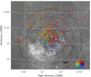 |
Fig. 9 Relative proper motion vectors of the stars in Berkeley 59 shown overplotted on a DSS red image. The color and direction of the bars extending from the black dots (the sources) indicate the direction of the movement. The concentric circles mark radii of (10, 20, 30, 40)′ from the center. The white star marks the highest surface density, which we took as the center. For a zoomed-in version see Fig. B.1. |
5.2.2 Radial component of the relative proper motion vector
Next, we estimated the behavior of the radial component of the relative proper motion vector (μr), defined as a projection of the relative proper motion vector onto the vector connecting the cluster center with the star in question. Positive values of μr indicate the radial stellar component pointing away from the center. In Fig. 11 we show μr as a function of distance from the cluster center. The sources are binned by radial distance with a bin size of 2′. The weighted mean and corresponding standard deviation of μr in each bin are shown in red. μr increases outward from the center up to a radius of about 20′. After this, the mean μr drops and remains roughly constant up to a radius of 30′. The change in behavior occurs at a similar distance from the cluster center, where the radial profile (Fig. 8) also shows a discontinuity. The increase in μr suggests a radially dependent expansion velocity in which more stars move faster outward the farther away they are from the center. We fit a line to the observed increasing trend and obtained a slope 0.022 ± 0.003 mas yr−1 arcmin−1 =0.37 ± 0.04 km s−1 pc−1. This is significantly higher than 0.1 ± 0.4 km s−1 pc−1 previously found by Kuhn et al. (2019), who performed a similar analysis, but only in the inner 3 pc (~10′) and based on only four bins.
In Fig. 12 we show the distribution of μr for the stars in the inner 18′. The median is found at 0.11 ± 0.02 mas yr−1 =0.52 ± 0.08 km s−1, indicating an expansion. Previously, Kuhn et al. (2019) derived a value of 0.34 ± 0.24 km s−1, or 0.33 ± 0.22 km s−1 if rescaled to the distance of 1009 pc. Because the uncertainties were large, Kuhn et al. (2019) concluded that the results on expansion/contraction for Berkeley 59 are ambiguous. Our member sample, which is several times larger than that used by Kuhn et al. (2019), yields a result with >6σ significance in favor of cluster expansion. The distribution is also asymmetric, with a small secondary peak to the right of the median, a hint of which can also be seen in Fig. 5.1 of Kuhn et al. (2019).
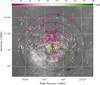 |
Fig. 10 Similar to Fig. 9. Here, the proper motion vectors are colored according to the angle between the line connecting the star to the center (white star) and its proper motion vector. Purple hues indicate a motion away from the center, and green hues a motion toward the center. White bars mark motion perpendicular to the line connecting the star to the center. White stars may move in opposite directions with respect to each other. |
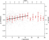 |
Fig. 11 Radial component of the relative proper motion (μr) as a function of distance from the center of Berkeley 59. The red points and error bars show the values of μr in 2′ bins, calculated as the weighted mean and standard deviation, respectively. A distance of 1009 pc was assumed for the top and right axes. Positive values of μr indicate expansion. The black line shows a linear fit to the red points inside the radius of 18′ and has a slope of 0.022 ± 0.003 mas yr−1 arcmin−1 and an intercept of 0.013 ± 0.028 mas yr−1. |
6 Properties of Berkeley 59
In this section, we concentrate on the central cluster of the region, Berkeley 59, and limit the analysis to the 18′ radius around the central position, as determined in Section 5.1.
6.1 Masses and ages from the HR diagram
We determined stellar ages and masses using the HR diagram (Fig. 6). To achieve this, we interpolated PARSEC isochrones for ages ranging from 0.1 Myr to 100 Myr in steps of 0.05 dex. To estimate the uncertainties in the derived parameters, we conducted a Monte Carlo simulation in which Teff and MJ were resampled based on their uncertainties. In the SED fittig procedure (Section 4.2), we assigned the uncertainties in Teff and AV equal to the step in the fitting grid (100 K and 0.25 mag, respectively). Teff and AV from the SED fitting appear to be correlated, however, as shown in Appendix C. We quantified this correlation using the global Pearson correlation coefficient computed across the full dataset. This coefficient was then used to construct a bivariate normal distribution for each star, centered on its derived (Teff, AV) values and incorporating the corresponding uncertainties. We drew 100 random samples per star from this distribution, and independently sampled the apparent J–band magnitudes using their reported errors. With this, we calculated a sample of 100 MJ values for each star. The uncertainty in distance was not considered in this calculation.
The Monte Carlo simulation described above resulted in mass and age distributions for each object. They were often non-Gaussian and can be significantly asymmetric. For the mass, we stored the derived distributions and later used them to generate random samples for deriving the IMF. For the age, we recorded the median values from 100 Monte Carlo iterations for each object. In total, we derived masses for 920 objects out of the 1030 high-probability candidate members. The remaining 110 objects either did not have a J–band measurement or had a poor SED fit.
As is commonly seen in HR diagrams of star-forming regions, objects in Berkeley 59 show a significant span in ages, with mean and median ages of 4.6 Myr and 2.9 Myr, respectively. The result is similar for the entire region or for the radius of 18′ around the center. The median age agrees with the age of ~2 Myr that is typically assumed for Berkeley 59 (Pandey et al. 2008).
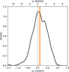 |
Fig. 12 Distribution of the radial component of the relative proper motion vector for Berkeley 59 (r ≤ 18′). The dashed gray line marks the velocity of zero, the vertical solid orange line represents the median of the distribution, and the orange shaded area spans a 3σ range around the median. |
6.2 Initial mass function
The IMF was derived using a procedure identical to that from Mužić et al. (2022), where the masses for each star were randomly sampled from the respective mass distributions obtained in Sect. 6.1, with additional bootstrapping. This resulted in 10 000 mass distributions, which were binned onto the same grid and then averaged. The bins were selected to contain a significant number of stars (typically 80–100), except for the highest-mass bin, which was more sparsely populated (~20 stars).
The IMF was derived for the mass range between 0.4 M⊙ and 7 M⊙. The low-mass limit was set by the estimated completeness limit (Section 2.2), and the high-mass limit stemmed from the upper Teff limit in the SED fitting (Section 4.2). In Appendix D, we examine the potential impact of the selection steps on the IMF derivation and conclude that within the chosen mass range, the selection process is not expected to introduce significant biases.
In Fig. 13, we show the derived IMF. We also show the standard IMF from Kroupa (2001), which is identical to the Salpeter (1955) IMF down to 0.5 M⊙. The fit to the data is in excellent agreement with the standard IMF. A power-law fit in the form dN/dM ∝ M−α yields the slope α = 2.3 ± 0.3. A similar slope (α = 2.33 ± 0.11.) was previously derived for the same cluster for a mass range between 0.2 and 28 M⊙ by Panwar et al. (2018).
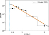 |
Fig. 13 Initial mass function of Berkeley 59. The solid orange line shows a power-law fit with a slope α = 2.3±0.2. The standard mass function from Kroupa (2001) normalized to match the total number of objects in our IMF derivation is shown by the dotted black line. The vertical dashed blue line marks the completeness limit. |
6.3 Velocity dispersion and relaxation timescale
We obtained a one-dimensional velocity dispersion σ1D by combining the velocity dispersions in right ascension and declination in quadrature (see Eq. (3) in Mužić et al. 2022). These were determined as the weighted standard deviations of the measured proper motions in the two directions. To ensure a robust velocity dispersion measurement, the proper motions were resampled 104 times, incorporating proper motion uncertainties, their correlations, and bootstrapping. This yielded σ1D = 0.25±0.03 mas yr−1, which is equivalent to 1.18±0.12 km s−1. This value agrees with σ1D=1.2±0.2 km s−1 derived by Kuhn et al. (2019).
The total mass of Berkeley 59 (out to the radius of 18’) and half-mass radius can be estimated using an MC simulation similar to the one we used to derive the IMF. We obtained a total mass of 650±30 M⊙, which is in principle a lower limit because of the completeness at the lower-mass end and the lack of sensitivity of the optical data to the more obscured YSO population. The half-mass radius rh=5.8 ± 0.4′, which is equivalent to 1.71 ± 0.13 pc at the distance of 1009 pc. Using the mass and the half-mass radius, we calculated the virial velocity dispersion σvir (Eq. (4) in Mužić et al. 2022). Assuming η=10, we obtained σvir=0.41 ± 0.02 km s−1. Lower values of η may be appropriate for clusters with γ < 3, however (Portegies Zwart et al. 2010). For η=5, we obtained σvir=0.57 ± 0.02 km s−1. In any case, the cluster currently appears to be supervirial.
Using the half-mass radius and the one-dimensional velocity dispersion, we calculated the crossing time (Binney & Tremaine 2008) as tcross ~ rh/σ1D = 1.4 ± 0.2 Myr. Combined with N=707 (number of probable members within r=18′), we derived the relaxation time (see Eq. (5) in Mužić et al. 2022) trelax ~15 ± 2 Myr. The relaxation time is significantly longer than the estimated cluster age. This suggests that the mass segregation reported by Panwar et al. (2018, 2024) is probably primordial and not a consequence of dynamical relaxation.
To assess whether the cluster might be affected by the Galactic potential, we compared its radius with its Jacobi (or Hill) radius (Binney & Tremaine 2008). To do this, we used Eq. (6) in Mužić et al. (2022), which requires the knowledge if the cluster mass and the Oort constants at its Galactic position. The latter can be estimated using the relations from Piskunov et al. (2007). We obtained a Jacobi radius rJ ~ 12.5 pc, which is more than twice as large as the outer cluster radius we determined in Section 5.1.
7 Summary and conclusions
We have studied a region with a radius of 2° in Cepheus OB4, centered on the young cluster Berkeley 59. Using a catalog that includes optical and near-infrared photometry, along with precise positions and proper motions from Gaia DR3, we applied the PRF algorithm to estimate the membership probabilities for each source within our field of view. The stellar masses and extinctions were determined by fitting SEDs to atmospheric models, and the membership was further refined by requiring a position in the HR diagram compatible with youth. Based on a list of 1030 probable members, we investigated the internal dynamics of the region relative to the mean proper motion of Berkeley 59. The main findings of this work are summarized below.
Most of the sources are concentrated within the cluster Berkeley 59 or scattered around it. Additionally, a small but distinct group of stars is found about 1° north of Berkeley 59, associated with the nebula NGC 7822 and located at a similar distance. We also identified a number of potentially young sources south of Berkeley 59 that roughly follow the filamentary structure of the molecular gas, but appear to be situated significantly behind Cepheus OB4;
The distance to Berkeley 59 estimated from Gaia DR3 parallaxes is 1009 ± 12 pc, and the median age is 2.9 Myr. This agrees with previous age estimates;
The radial profile of Berkeley 59 was fit with the EFF profile (Elson et al. 1987), which returned a peak stellar surface density Σ0 = 14 ± 1.9 stars arcmin−2 and a (King profile) core radius rc = 0.50 ± 0.07 pc. We estimate that the cluster extends out to a radius of ~18 arcmin, which is equivalent to ~5 pc at a distance of 1009 pc;
Berkeley 59 shows an expansion pattern with an expansion velocity that increases with radius. The median of the distribution of the radial component of the relative proper motion vector (μr) out to r= 18′ is at 0.11 ± 0.02 mas yr−1, which is equivalent to vr = 0.52 ± 0.08 km s−1 at a distance of 1009 pc, that is, the expansion is confirmed with a statistical significance of > 6σ. Moreover, the detected expansion pattern is asymmetric, with the preferred direction toward the north. This agrees with the findings of Wright et al. (2024), who reported that most expanding young clusters and OB associations exhibit asymmetric expansion;
The IMF between 0.4 and 7 M⊙ is well represented by a single power law (dN/dM ∝ M−α), with the slope α = 2.3±0.3, close to Salpeter’s slope and in agreement with previous works in the same region;
The velocity dispersion of Berkeley 59 is well above the virial velocity dispersion derived from the total mass (650 ± 30 M⊙) and half-mass radius (1.71 ± 0.13 pc);
The relaxation timescale is several times longer than the estimated age of Berkeley 59, suggesting that the cluster is still not dynamically relaxed;
The proper motions of the sources in the nebula NGC 7822 (cluster 0 in Mintz et al. 2021) point away from Berkeley 59. This region also contains a larger fraction of Class I sources than Berkeley 59 (Mintz et al. 2021), suggesting that it may have been triggered by expansion of the HII region.
Data availability
Table 3 is available at the CDS via https://cdsarc.cds.unistra.fr/viz-bin/cat/J/A+A/703/A193.
Acknowledgements
We thank Santiago González Gaitán and the anonymous referee for valuable discussions and insightful suggestions that improved the quality of this work. K.M. acknowledges support from the Fundação para a Ciência e a Tecnologia (FCT) through the CEEC-individual contract 2022.03809.CEECIND and research grants UIDB/04434/2020 and UIDP/04434/2020, and the Scientific Visitor Programme of the European Southern Observatory (ESO) in Chile. V.A-A acknowledges support from the INAF grant 1.05.12.05.03. This work has made use of data from the European Space Agency (ESA) mission Gaia (https://www.cosmos.esa.int/gaia), processed by the Gaia Data Processing and Analysis Consortium (DPAC, https://www.cosmos.esa.int/web/gaia/dpac/consortium). Funding for the DPAC has been provided by national institutions, in particular the institutions participating in the Gaia Multilateral Agreement. This publication makes use of VOSA, developed under the Spanish Virtual Observatory (https://svo.cab.inta-csic.es) project funded by MCIN/AEI/10.13039/501100011033/ through grant PID2020-112949GB-I00. VOSA has been partially updated by using funding from the European Union’s Horizon 2020 Research and Innovation Programme, under Grant Agreement no. 776403 (EXOPLANETS-A).
References
- Allard, F., Homeier, D., & Freytag, B. 2011, in Astronomical Society of the Pacific Conference Series, 448, 16th Cambridge Workshop on Cool Stars, Stellar Systems, and the Sun, eds. C. Johns-Krull, M. K. Browning, & A. A. West, 91 [Google Scholar]
- Armstrong, J. J., & Tan, J. C. 2024, A&A, 692, A166 [NASA ADS] [CrossRef] [EDP Sciences] [Google Scholar]
- Armstrong, J. J., Wright, N. J., Jeffries, R. D., Jackson, R. J., & Cantat-Gaudin, T. 2022, MNRAS, 517, 5704 [NASA ADS] [CrossRef] [Google Scholar]
- Bailer-Jones, C. A. L. 2011, MNRAS, 411, 435 [Google Scholar]
- Baraffe, I., Homeier, D., Allard, F., & Chabrier, G. 2015, A&A, 577, A42 [NASA ADS] [CrossRef] [EDP Sciences] [Google Scholar]
- Bayo, A., Barrado, D., Allard, F., et al. 2017, MNRAS, 465, 760 [Google Scholar]
- Binney, J., & Tremaine, S. 2008, Galactic Dynamics, 2nd edn. (Princeton, NJ: Princeton University Press) [Google Scholar]
- Bressan, A., Marigo, P., Girardi, L., et al. 2012, MNRAS, 427, 127 [NASA ADS] [CrossRef] [Google Scholar]
- Cantat-Gaudin, T., Jordi, C., Vallenari, A., et al. 2018, A&A, 618, A93 [NASA ADS] [CrossRef] [EDP Sciences] [Google Scholar]
- Cantat-Gaudin, T., Jordi, C., Wright, N. J., et al. 2019, A&A, 626, A17 [NASA ADS] [CrossRef] [EDP Sciences] [Google Scholar]
- Conrad, C., Scholz, R. D., Kharchenko, N. V., et al. 2017, A&A, 600, A106 [NASA ADS] [CrossRef] [EDP Sciences] [Google Scholar]
- Della Croce, A., Dalessandro, E., Livernois, A., & Vesperini, E. 2024, A&A, 683, A10 [NASA ADS] [CrossRef] [EDP Sciences] [Google Scholar]
- Elson, R. A. W., Fall, S. M., & Freeman, K. C. 1987, ApJ, 323, 54 [Google Scholar]
- Eswaraiah, C., Pandey, A. K., Maheswar, G., et al. 2012, MNRAS, 419, 2587 [NASA ADS] [CrossRef] [Google Scholar]
- Flewelling, H. 2017, in American Astronomical Society Meeting Abstracts, 229, American Astronomical Society Meeting Abstracts #229, 237.07 [Google Scholar]
- Gahm, G. F., Wilhelm, M. J. C., Persson, C. M., Djupvik, A. A., & Portegies Zwart, S. F. 2022, A&A, 663, A111 [NASA ADS] [CrossRef] [EDP Sciences] [Google Scholar]
- Gaia Collaboration (Prusti, T., et al.) 2016, A&A, 595, A1 [NASA ADS] [CrossRef] [EDP Sciences] [Google Scholar]
- Gaia Collaboration (Helmi, A., et al.) 2018, A&A, 616, A12 [NASA ADS] [CrossRef] [EDP Sciences] [Google Scholar]
- Gaia Collaboration (Vallenari, A., et al.) 2023, A&A, 674, A1 [NASA ADS] [CrossRef] [EDP Sciences] [Google Scholar]
- Getman, K. V., Broos, P. S., Kuhn, M. A., et al. 2017, ApJS, 229, 28 [Google Scholar]
- Goodwin, S. P., & Bastian, N. 2006, MNRAS, 373, 752 [Google Scholar]
- Guilherme-Garcia, P., Krone-Martins, A., & Moitinho, A. 2023, A&A, 673, A128 [NASA ADS] [CrossRef] [EDP Sciences] [Google Scholar]
- Gutermuth, R. A., Megeath, S. T., Myers, P. C., et al. 2009, ApJS, 184, 18 [Google Scholar]
- Inutsuka, S.-i., Inoue, T., Iwasaki, K., & Hosokawa, T. 2015, A&A, 580, A49 [NASA ADS] [CrossRef] [EDP Sciences] [Google Scholar]
- Kharchenko, N. V., Scholz, R. D., Piskunov, A. E., Röser, S., & Schilbach, E. 2007, Astron. Nachr., 328, 889 [Google Scholar]
- King, I. R. 1966, AJ, 71, 276 [NASA ADS] [CrossRef] [Google Scholar]
- Koenig, X. P., Leisawitz, D. T., Benford, D. J., et al. 2012, ApJ, 744, 130 [Google Scholar]
- Kroupa, P. 2001, MNRAS, 322, 231 [NASA ADS] [CrossRef] [Google Scholar]
- Kun, M., Kiss, Z. T., & Balog, Z. 2008, in Handbook of Star Forming Regions, Volume I, 4, ed. B. Reipurth, 136 [Google Scholar]
- Kuhn, M. A., Feigelson, E. D., Getman, K. V., et al. 2014, ApJ, 787, 107 [Google Scholar]
- Kuhn, M. A., Getman, K. V., Feigelson, E. D., et al. 2017, AJ, 154, 214 [NASA ADS] [CrossRef] [Google Scholar]
- Kuhn, M. A., Hillenbrand, L. A., Sills, A., Feigelson, E. D., & Getman, K. V. 2019, ApJ, 870, 32 [CrossRef] [Google Scholar]
- Lada, C. J., & Lada, E. A. 2003, ARA&A, 41, 57 [Google Scholar]
- Lemaitre, G., Nogueira, F., & Aridas, C. K. 2016, arXiv e-prints [arXiv:1609.06570] [Google Scholar]
- Lim, B., Nazé, Y., Hong, J., et al. 2021, AJ, 162, 56 [NASA ADS] [CrossRef] [Google Scholar]
- Lindegren, L., Bastian, U., Biermann, M., et al. 2021, A&A, 649, A4 [EDP Sciences] [Google Scholar]
- Lozinskaya, T. A., Sitnik, T. G., & Toropova, M. S. 1987, Soviet Ast., 31, 493 [NASA ADS] [Google Scholar]
- Majaess, D. J., Turner, D. G., Lane, D. J., & Moncrieff, K. E. 2008, The Journal of the American Association of Variable Star Observers, 36, 90 [Google Scholar]
- Matthews, B. 1975, Biochim. Biophys. Acta Protein Struct., 405, 442 [Google Scholar]
- Meingast, S., Alves, J., & Rottensteiner, A. 2021, A&A, 645, A84 [NASA ADS] [CrossRef] [EDP Sciences] [Google Scholar]
- Mintz, A., Hora, J. L., & Winston, E. 2021, AJ, 162, 236 [NASA ADS] [CrossRef] [Google Scholar]
- Miret-Roig, N., Bouy, H., Olivares, J., et al. 2019, A&A, 631, A57 [NASA ADS] [CrossRef] [EDP Sciences] [Google Scholar]
- Mužić, K., Scholz, A., Peña Ramírez, K., et al. 2019, ApJ, 881, 79 [Google Scholar]
- Mužić, K., Almendros-Abad, V., Bouy, H., et al. 2022, A&A, 668, A19 [NASA ADS] [CrossRef] [EDP Sciences] [Google Scholar]
- Ogura, K., Sugitani, K., & Pickles, A. 2002, AJ, 123, 2597 [Google Scholar]
- Pandey, A. K., Sharma, S., Ogura, K., et al. 2008, MNRAS, 383, 1241 [Google Scholar]
- Pang, X., Li, Y., Yu, Z., et al. 2021, ApJ, 912, 162 [NASA ADS] [CrossRef] [Google Scholar]
- Panwar, N., Pandey, A. K., Samal, M. R., et al. 2018, AJ, 155, 44 [NASA ADS] [CrossRef] [Google Scholar]
- Panwar, N., Rishi, C., Sharma, S., et al. 2024, arXiv e-prints [arXiv:2406.08261] [Google Scholar]
- Parker, R. J., Wright, N. J., Goodwin, S. P., & Meyer, M. R. 2014, MNRAS, 438, 620 [Google Scholar]
- Pastorelli, G., Marigo, P., Girardi, L., et al. 2020, MNRAS, 498, 3283 [Google Scholar]
- Piskunov, A. E., Schilbach, E., Kharchenko, N. V., Röser, S., & Scholz, R. D. 2007, A&A, 468, 151 [NASA ADS] [CrossRef] [EDP Sciences] [Google Scholar]
- Planck Collaboration XI. 2016, AAP, 594, A11 [Google Scholar]
- Portegies Zwart, S. F., McMillan, S. L. W., & Gieles, M. 2010, ARA&A, 48, 431 [NASA ADS] [CrossRef] [Google Scholar]
- Reis, I., Baron, D., & Shahaf, S. 2019, AJ, 157, 16 [Google Scholar]
- Rossano, G. S., Grayzeck, E. J., & Angerhofer, P. E. 1983, AJ, 88, 1835 [NASA ADS] [CrossRef] [Google Scholar]
- Rosvick, J. M., & Majaess, D. 2013, AJ, 146, 142 [NASA ADS] [CrossRef] [Google Scholar]
- Salpeter, E. E. 1955, ApJ, 121, 161 [Google Scholar]
- Sills, A., Rieder, S., Scora, J., McCloskey, J., & Jaffa, S. 2018, MNRAS, 477, 1903 [Google Scholar]
- Skiff, B. A. 2014, VizieR Online Data Catalog: Catalogue of Stellar Spectral Classifications (Skiff, 2009–2014), VizieR On-line Data Catalog: B/mk. Originally published in: 2014yCat....1.2023S [Google Scholar]
- Skrutskie, M. F., Cutri, R. M., Stiening, R., et al. 2006, AJ, 131, 1163 [NASA ADS] [CrossRef] [Google Scholar]
- Sugitani, K., Fukui, Y., & Ogura, K. 1991, ApJS, 77, 59 [NASA ADS] [CrossRef] [Google Scholar]
- Tan, J. C. 2000, ApJ, 536, 173 [NASA ADS] [CrossRef] [Google Scholar]
- Taylor, M. B. 2005, in Astronomical Society of the Pacific Conference Series, 347, Astronomical Data Analysis Software and Systems XIV, eds. P. Shopbell, M. Britton, & R. Ebert, 29 [Google Scholar]
- van Leeuwen, F. 2009, A&A, 497, 209 [CrossRef] [EDP Sciences] [Google Scholar]
- Wenger, M., Ochsenbein, F., Egret, D., et al. 2000, A&AS, 143, 9 [NASA ADS] [CrossRef] [EDP Sciences] [Google Scholar]
- Wright, N. J. 2020, New A Rev., 90, 101549 [NASA ADS] [CrossRef] [Google Scholar]
- Wright, N. J., Jeffries, R. D., Jackson, R. J., et al. 2019, MNRAS, 486, 2477 [CrossRef] [Google Scholar]
- Wright, N. J., Jeffries, R. D., Jackson, R. J., et al. 2024, MNRAS, 533, 705 [NASA ADS] [CrossRef] [Google Scholar]
- Yu, J., Khanna, S., Themessl, N., et al. 2023, ApJS, 264, 41 [NASA ADS] [CrossRef] [Google Scholar]
- Zari, E., Brown, A. G. A., & de Zeeuw, P. T. 2019, A&A, 628, A123 [NASA ADS] [CrossRef] [EDP Sciences] [Google Scholar]
As noted before by Bayo et al. (2017); Mužić et al. (2022), for instance, the SED fitting process is not highly sensitive to log(g), resulting in flat probability density distributions in the range we examined.
Appendix A PRF scores and feature importance
In Table A.1 we show the details of the 6 PRF runs, along with the scores obtained through cross-validation (see Section 3.2.2). The scores are also shown in Fig. A.1. In Fig. A.2, we show the relative importance of the 17 used features as returned by the classifier in run F. Corresponding plots from other runs look very similar to this one. The uncertainties correspond to the standard deviation of the 50 split values.
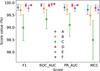 |
Fig. A.1 Metrics of the six different runs of the PRF (see Table A.1 for IDs, run details and the exact score values). Points are offset on the x-axis for clarity. |
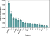 |
Fig. A.2 Relative feature importance, evaluated for the classifier of run F. The error bars are the standard deviation of the 50 random split samples used to evaluate each classifier. |
Parameters of the sampling strategy for each run of the PRF and the corresponding scores.
Appendix B Relative Proper Motions in various regions
In Figs. B.1 and B.2, we show the zoom-in versions of Fig. 9, which allows appreciation of details in relative proper motions for Berkeley 59 and the region ~1° north of it, associated with the nebula NGC 7822 (Cluster 0 in Mintz et al. 2021 and BLR2 in Sugitani et al. 1991; Ogura et al. 2002).
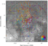 |
Fig. B.1 Same as Fig. 9, but focused on the cluster Berkeley 59. The circle marks the 18′ radius, which we adopted as the cluster radius. |
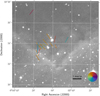 |
Fig. B.2 Same as Fig. 9, but focused on the small region associated with the nebula to the north of the cluster. |
Appendix C Correlation between Teff and AV from SED fitting
In Section 4.2, we derived Teff and AV by fitting each star’s SED to the atmosphere models. As shown in Fig C.1, these two parameters show some degree of correlation, which is commonly seen in SED fitting using optical/near-infrared multiband photometry (Bailer-Jones 2011; Bayo et al. 2017; Yu et al. 2023).
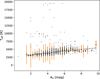 |
Fig. C.1 The relationship between the Teff and AV obtained from the SED fitting in Section 4.2 (black dots). The orange points represent the median value Teff values at each step of the extinction grid, with error bars indicating the standard deviation. The blue dashed line corresponds to a linear fit to the orange points. |
Appendix D IMF selection function
Figure D.1 summarizes how the number of objects evolves through successive selection steps, shown as a function of J–band magnitude. For this analysis, we excluded sources with declination below 66.8°, as they are not included in the IMF calculation, which is the main focus here. We use the J–band magnitude because our mass estimates are derived from the HR diagram constructed in that band.
The top panel shows the fraction of sources that pass the PRF-based selection, identifying high-probability members (Section 4.1. The middle and right panels present statistics relative to this sample: the middle panel shows the percentage of PRF-selected sources that also meet the HRD age cut (30 Myr limit; see Section 4.2, orange) and have mass estimates (gray; see Section 6.1). The bottom panel shows the corresponding absolute number of these surviving sources per magnitude bin.
The decrease in the number of objects at J ≲ 11 mag results from the upper limit on effective temperature during the SED fitting (Section 4.2). At the low-mass end, there is a sharp drop in the number of objects at J > 16, which corresponds to masses ≲ 0.25 M⊙ for the distance of Berkeley 59, age of 2 Myr, and the average extinction of AV = 4 mag. For the lowest-mass bin in our IMF calculation (0.4-0.6 M⊙), the number of the removed objects is small, at most about 20%.
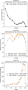 |
Fig. D.1 Selection effects as a function of J–band magnitude across different stages of the sample construction. For this plot, we removed the southern part of the field (δ < 66.8°). Top: Fraction of objects surviving the main selection step (PRF classification). Middle: Percentage of objects remaining at each magnitude step relative to the sample of probable members from the PRF run. The orange symbols show the percentage of surviving objects after removing the objects older than 30 Myr (Section. 4.2), and the gray symbols show those with valid mass estimates (Section. 6.1). Bottom: Same as the middle panel, but showing the number of objects instead of percentages. Tick marks on the top x-axis indicate approximate stellar masses corresponding to J–band magnitudes at the distance of Berkeley 59, age of 2 Myr and extinction AV = 4 mag. |
All Tables
Parameters of the sampling strategy for each run of the PRF and the corresponding scores.
All Figures
|
Fig. 1 Density of sources in our final catalog as a function of magnitude. |
| In the text | |
|
Fig. 2 Gaia DR3 proper motions of objects in Cepheus OB4 (gray dots). The black dots represent the 860 candidate members from the literature within a radius of 30′ from the center of Berkeley 59. The orange ellipse indicates the proper motion selection criterion for constructing the member training set. In the lower right corner, we show the mean proper motion uncertainty. |
| In the text | |
|
Fig. 3 Color–magnitude diagrams we used to select the training set. The black dots in the top panels show candidate members from the literature, and the gray dots mark all the sources in the field. The dashed lines show the selection criteria, and the solid lines represent the 2 Myr PARSEC isochrones, shifted to a distance of 1100 pc (Kuhn et al. 2019). In the lower panels, the black dots represent the probable members we selected for the training set after the proper motion, color, and parallax filters. |
| In the text | |
|
Fig. 4 Parallax measurements for the candidates of the member training set, selected based on proper motions and colors (black dots). The dotted orange line represents the weighted average of the parallaxes, and the shaded area marks the ±1σ range. The red crosses mark the sources that were excluded from the final member training set (see text for the details of the criterion we applied). |
| In the text | |
|
Fig. 5 Distribution of the membership probability of the final catalog limited to objects 30′ from the center for clarity. The four leftmost columns are capped for better readability. The inset diagram shows the prediction for all objects labeled as members in the training set. The rightmost column of the inset diagram is capped, and its value is depicted next to it. |
| In the text | |
|
Fig. 6 Hertzsprung-Russell diagram showing the candidates with membership probabilities ≥90% (black dots). The blue crosses mark candidates located in the southern filaments (see Sect. 4.3). The isochrones (solid gray lines) and the lines of constant mass (dashed orange lines) are from the PARSEC series (Bressan et al. 2012; Pastorelli et al. 2020). A typical error bar is shown in the lower left corner. Objects located below the 30 Myr isochrone are considered contaminants. The right panel is the zoomed-in version of the left panel. |
| In the text | |
|
Fig. 7 Sources with membership probabilities ≥90% and consistent with ages <30 Myr (black dots) overplotted on the Planck 857 GHz image (left) and DSS red image (right) of the region around Berkeley 56. The sources that are likely located in the background, associated with the southern filaments, are marked with blue crosses. The solid orange circle encompasses the entire region (r=2°), the dashed blue circle shows the region in which the training sample was selected (r=30′), and the dotted black circle shows an extent of the cluster as derived from the radial profile (r=18′). The white star shows the position of the center of Berkeley 59 derived in Section 5.1. |
| In the text | |
|
Fig. 8 Radial profile of Berkeley 59 in logarithmic scale. Each black dot shows the surface density of its corresponding annulus about the center. The dashed orange line is the best-fit EFF profile (Elson et al. 1987) up to a radius of 30′ (dotted gray line). The vertical dashed line represents the core radius derived from the profile fitting, and the dotted line marks the approximate outer radius of the cluster (r=18′). |
| In the text | |
|
Fig. 9 Relative proper motion vectors of the stars in Berkeley 59 shown overplotted on a DSS red image. The color and direction of the bars extending from the black dots (the sources) indicate the direction of the movement. The concentric circles mark radii of (10, 20, 30, 40)′ from the center. The white star marks the highest surface density, which we took as the center. For a zoomed-in version see Fig. B.1. |
| In the text | |
|
Fig. 10 Similar to Fig. 9. Here, the proper motion vectors are colored according to the angle between the line connecting the star to the center (white star) and its proper motion vector. Purple hues indicate a motion away from the center, and green hues a motion toward the center. White bars mark motion perpendicular to the line connecting the star to the center. White stars may move in opposite directions with respect to each other. |
| In the text | |
|
Fig. 11 Radial component of the relative proper motion (μr) as a function of distance from the center of Berkeley 59. The red points and error bars show the values of μr in 2′ bins, calculated as the weighted mean and standard deviation, respectively. A distance of 1009 pc was assumed for the top and right axes. Positive values of μr indicate expansion. The black line shows a linear fit to the red points inside the radius of 18′ and has a slope of 0.022 ± 0.003 mas yr−1 arcmin−1 and an intercept of 0.013 ± 0.028 mas yr−1. |
| In the text | |
|
Fig. 12 Distribution of the radial component of the relative proper motion vector for Berkeley 59 (r ≤ 18′). The dashed gray line marks the velocity of zero, the vertical solid orange line represents the median of the distribution, and the orange shaded area spans a 3σ range around the median. |
| In the text | |
|
Fig. 13 Initial mass function of Berkeley 59. The solid orange line shows a power-law fit with a slope α = 2.3±0.2. The standard mass function from Kroupa (2001) normalized to match the total number of objects in our IMF derivation is shown by the dotted black line. The vertical dashed blue line marks the completeness limit. |
| In the text | |
|
Fig. A.1 Metrics of the six different runs of the PRF (see Table A.1 for IDs, run details and the exact score values). Points are offset on the x-axis for clarity. |
| In the text | |
|
Fig. A.2 Relative feature importance, evaluated for the classifier of run F. The error bars are the standard deviation of the 50 random split samples used to evaluate each classifier. |
| In the text | |
|
Fig. B.1 Same as Fig. 9, but focused on the cluster Berkeley 59. The circle marks the 18′ radius, which we adopted as the cluster radius. |
| In the text | |
|
Fig. B.2 Same as Fig. 9, but focused on the small region associated with the nebula to the north of the cluster. |
| In the text | |
|
Fig. C.1 The relationship between the Teff and AV obtained from the SED fitting in Section 4.2 (black dots). The orange points represent the median value Teff values at each step of the extinction grid, with error bars indicating the standard deviation. The blue dashed line corresponds to a linear fit to the orange points. |
| In the text | |
|
Fig. D.1 Selection effects as a function of J–band magnitude across different stages of the sample construction. For this plot, we removed the southern part of the field (δ < 66.8°). Top: Fraction of objects surviving the main selection step (PRF classification). Middle: Percentage of objects remaining at each magnitude step relative to the sample of probable members from the PRF run. The orange symbols show the percentage of surviving objects after removing the objects older than 30 Myr (Section. 4.2), and the gray symbols show those with valid mass estimates (Section. 6.1). Bottom: Same as the middle panel, but showing the number of objects instead of percentages. Tick marks on the top x-axis indicate approximate stellar masses corresponding to J–band magnitudes at the distance of Berkeley 59, age of 2 Myr and extinction AV = 4 mag. |
| In the text | |
Current usage metrics show cumulative count of Article Views (full-text article views including HTML views, PDF and ePub downloads, according to the available data) and Abstracts Views on Vision4Press platform.
Data correspond to usage on the plateform after 2015. The current usage metrics is available 48-96 hours after online publication and is updated daily on week days.
Initial download of the metrics may take a while.