| Issue |
A&A
Volume 707, March 2026
|
|
|---|---|---|
| Article Number | A296 | |
| Number of page(s) | 22 | |
| Section | Interstellar and circumstellar matter | |
| DOI | https://doi.org/10.1051/0004-6361/202557408 | |
| Published online | 23 March 2026 | |
The role of detailed gas and dust opacities in shaping the evolution of the inner disc edge subject to episodic accretion
1
Max Planck Institute for Astronomy (MPIA),
Königstuhl 17,
69117
Heidelberg,
Germany
2
Fakultät für Physik und Astronomie, Universität Heidelberg,
Im Neuenheimer Feld 226,
69120
Heidelberg,
Germany
3
Fakultät für Physik, Universität Duisburg-Essen,
Lotharstraße 1,
47057
Duisburg,
Germany
4
Ludwig-Maximilians-Universität München, Universitäts-Sternwarte,
Scheinerstr 1,
81679
München,
Germany
★ Corresponding author: This email address is being protected from spambots. You need JavaScript enabled to view it.
Received:
25
September
2025
Accepted:
11
February
2026
Abstract
Context. The transition in turbulence in the inner regions of protoplanetary discs and the closely connected dust sublimation front lead to a periodic instability, manifesting as episodic accretion outbursts. For the corresponding interplay between heating and cooling, the opacity of the material needs to be treated carefully.
Aims. We investigated the effects of different dust and gas opacity descriptions on the structure and evolution of the inner regions of protoplanetary discs. The effect on the episodic instability of the inner disc edge is of central interest here.
Methods. Two-dimensional (2D) axisymmetric radiation hydrodynamic models were employed to simulate the evolution of the inner disc over the course of several thousand years. Our simulations greatly expand on previously published models by implementing detailed descriptions of the gas and dust opacities in terms of their mean and frequency-dependent values. This allowed us to also consider binned frequency-dependent irradiation from the central star.
Results. The adaptive opacity description affects the structure of the inner disc rim to a great extent, and the contribution of the gas opacities is the most significant effect. The resulting effects include the shift in position of the dust sublimation front and the dead zone inner edge (DZIE), a significantly altered temperature in the dust-free region, and the manifestation of the equilibrium temperature degeneracy as a sharp temperature transition. The episodic instability due to the activation of the magneto-rotational instability in the dead zone still occurs, but at lower inner disc densities. While the gas opacities set the initial conditions for the instability by determining the location of the DZIE, the evolution of the outburst itself is mainly governed by the dust opacities. The analysis of criteria for non-axisymmetric instabilities reveals a possible breaking of the density peaks that is produced during the burst phase. However, due to the periodicity of the instability cycle, the DZIE itself may remain stable throughout the quiescent phases according to linear criteria applied to our axisymmetric models.
Conclusions. Although the thermal structure of the inner disc is crucially affected by different opacity descriptions, especially by the contribution of gas, the mechanism of the periodic instability of the DZIE remains active and is only marginally affected by the gas opacities. The observational consequences of the severely altered temperatures can be significant and require further investigation.
Key words: accretion, accretion disks / hydrodynamics / opacity / radiative transfer / protoplanetary disks / stars: protostars
© The Authors 2026
 Open Access article, published by EDP Sciences, under the terms of the Creative Commons Attribution License (https://creativecommons.org/licenses/by/4.0), which permits unrestricted use, distribution, and reproduction in any medium, provided the original work is properly cited.
This article is published in open access under the Subscribe to Open model.
Open Access funding provided by Max Planck Society.
1 Introduction
A substantial number of previous investigations has shown that the structure of the inner regions of protoplanetary discs is subject to extensive variability, originating from various processes and often manifesting as periodic outbursts of accretion onto the central star (Lin et al. 1985; Kley et al. 1999; Wunsch et al. 2006; Vorobyov & Basu 2006; Bae et al. 2013; Audard et al. 2014; Kadam et al. 2019; Steiner et al. 2021). A compilation of observed variable young stellar objects is provided in the Outbursting Young Stellar Objects Catalogue (OYCAT, Contreras Peña et al. 2025). The instabilities underlying the variability, and the potential luminosity feedback from the accretion burst, can significantly affect the thermal and chemical disc structure (Rab et al. 2017; Vorobyov et al. 2020; Laznevoi et al. 2025). While most previous studies focused on modelling observational signatures of outbursting young stellar objects such as FU Orionis (Herbig 1977), our previous work (Cecil & Flock 2024, hereafter Paper I) investigated the instability of the inner disc as an intrinsic consequence of the dynamic and thermal evolution of the region around the dead zone inner edge (DZIE) over long periods of time. A particular focus was thereby laid on the potential effects on the formation of planetesimals and planets in the inner disc.
The mechanism emerging in our radiation hydrodynamic simulations causes thermal instability (TI) by activating the magneto-rotational instability (MRI; Balbus & Hawley 1991) within the dead zone. While multiple previous studies have investigated such MRI-triggered outbursts (Zhu et al. 2009b; Kadam et al. 2020; Vorobyov et al. 2021; Cleaver et al. 2023; Das et al. 2025), Paper I showed that they can naturally arise from the turbulence transition between the irradiation-dominated gaseous inner disc and the optically thick outer domain. After activating the MRI beyond the DZIE, heating fronts travel into the dead zone, expanding the highly turbulent region and flushing large amounts of material onto the star. The burst phase is hereby substructured into multiple reflares of the instability. After the density of the inner regions has been lowered enough to prevent further MRI activation, the disc enters a quiescent phase, during which the inner dead zone is refilled with matter accreted from the outer regions. A new outburst cycle commences as soon as the combination of viscous heating and heat trapping again raises the midplane temperature above the MRI activation threshold beyond the DZIE. The temperatures reached during this burst process are not high enough to induce the classical TI by hydrogen ionisation (Bell & Lin 1994; Zhu et al. 2009a; Nayakshin et al. 2024; Elbakyan et al. 2024, 2025).
The type of accretion burst analysed in Paper I followed a limit cycle and could be tracked on S-curves of thermal stability, as was done in studies of cataclysmic variables (Lasota 2001; Hameury 2020; Jordan et al. 2024), but also for instabilities in protoplanetary discs (Martin & Lubow 2011; Nayakshin et al. 2024). Additionally, the burst cycle produced multiple pressure maxima, in which dust might accumulate and grow (Taki et al. 2016; Dullemond et al. 2018; Lee et al. 2022). On the other hand, the pebble- and planet-trapping pressure bump at the DZIE (Dzyurkevich et al. 2010; Flock et al. 2019; Chrenko et al. 2022) was periodically destroyed.
In Paper I, we used a simplified description of the opacities by fixing a single value for the gas contribution and two constant values for the mean and irradiation opacities for the dust coefficients. However, in the context of instability cycles, the opacities govern the critical surface densities for activating ( ) and shutting down (
 ) the underlying physical mechanism (MRI, in the case of Paper I; Lodato & Clarke 2004; Wunsch et al. 2006; Nayakshin et al. 2024). Furthermore, in regions in which dust sublimation becomes relevant, the gas opacity can be dominant in describing heating and cooling as well as determining the optical thickness of the disc material and the shape of the inner dust rim (Muzerolle et al. 2004; Isella & Natta 2005; Isella et al. 2006; Zhang & Tan 2011; Kuiper & Yorke 2012; Flock et al. 2016). Therefore, we expand our previous models by implementing detailed descriptions of the dust and gas opacities in this work. While several versions of relevant gas opacity calculations were presented in the literature (Helling et al. 2000; Ferguson et al. 2005; Marigo et al. 2024), Malygin et al. (2014) provided frequency-dependent opacities in addition to the Planck and Rosseland means. This allowed us to treat the irradiation in a frequency-dependent manner with contributions from the gas in addition to the frequency-dependent dust opacities, which have already been shown to result in a more accurate description of radiative transport in irradiated discs (Kuiper & Klessen 2013). The mean gas opacities by Malygin et al. (2014) were also used by Pavlyuchenkov et al. (2023) to show the multivalued equilibrium temperature solution leading to variable accretion, similar to the classical TI.
The density structure resulting from the burst cycle can be favourable for convergent migration of planetesimals, which has been proposed as a possible origin of the terrestrial planet distribution in the Solar System (Ogihara et al. 2018; Broz et al. 2021). However, the sharpness of the density features produced by the outburst mechanism calls their dynamic stability into question, especially regarding the Rossby wave instability (RWI; Lovelace et al. 1999). The RWI can lead to the emergence of large-scale vortices (Lyra & Low 2012; Bae et al. 2015; Flock et al. 2015), which can affect the dynamic disc structure, and which have been suggested as origins of dusty non-axisymmetric structures in discs observed with ALMA (e.g. Pérez et al. 2018; Ziampras et al. 2025b). Therefore, a careful investigation of the dynamic stability of spikes and bumps in the density structure during the burst and post-burst phases is warranted.
Our study intends to broaden our understanding of the inner disc structure and dynamic evolution under the effect of periodic instability by carefully treating dust and gas opacities in their mean and frequency-dependent form. Analogously to Paper I, we used 2D axisymmetric radiation hydrodynamic simulations, which were additionally complemented by the consideration of accretion luminosity feedback from the central host star. By subsequently activating the different descriptions in our simulations, we analysed their direct or combined impact. Additionally, we investigated the possibility of a non-axisymmetric instability of the density features produced by the burst cycles.
The paper is structured as follows. In Sect. 2, we describe the physical and numerical configuration of our models. We present the results of the simulations in Sect. 3 and discuss and analyse them further in Sect. 4. Our conclusions are summarised in Sect. 5.
2 Method
The set-up and execution of the simulations we conducted followed the same strategy as presented in Paper I. Section 2.1 gives a brief overview of the governing equations and summarises the main parts of the modelling procedure. The subsequent sections are mainly concerned with the extension of the models of Paper I by implementing new physical prescriptions. Section 2.2 presents the descriptions of gas and dust opacities, which are then included in the formulation of the frequency-dependent irradiation flux in Sect. 2.3. Section 2.4 describes the implementation of the turbulent viscosity and Sect. 2.5 addresses the numerical details. All simulations were conducted with the PLUTO code (Mignone et al. 2007), including the flux-limited diffusion (FLD) description of radiative transport presented in Flock et al. (2013).
2.1 Governing equations
The initial model of the 2D axisymmetric disc in spherical co-ordinates (r,θ,φ) was constructed by solving the equations of vertical hydrostatic equilibrium in conjunction with the two radiative transport equations in the FLD approximation, including viscous heat dissipation as a source term,
![Mathematical equation: \frac{1}{\gamma -1} \, \pder[P_\mathrm{g}]{t}=-\kappa_\mathrm{P} \, \rho \, c \, (a_\mathrm{R} \, T_\mathrm{g}^4 - E_\mathrm{R}) - \nabla \cdot F_\mathrm{irr} + Q_\mathrm{acc} , \label{eq:rad1} \\](/articles/aa/full_html/2026/03/aa57408-25/aa57408-25-eq3.png) (1)
(1)
![Mathematical equation: &\pder[E_\mathrm{R}]{t} - \nabla \cdot \left ( \frac{c \, \lambda}{\kappa_\mathrm{R} \, \rho} \, \nabla E_\mathrm{R} \right ) = \kappa_\mathrm{P} \, \rho\, c \, (a_\mathrm{R} \, T_\mathrm{g}^4 - E_\mathrm{R}) , \label{eq:rad2}](/articles/aa/full_html/2026/03/aa57408-25/aa57408-25-eq4.png) (2)
(2)
with the adiabatic factor γ, the gas thermal pressure Pg, the mass density ρ, the gas temperature Tg (which we assume to be equivalent to the dust temperature), the radiation energy density ER, the azimuthal component of the viscous stress tensor Qacc, the flux-limiter function λ (Levermore & Pomraning 1981), the radiation constant aR and the speed of light c. The description of the Planck and Rosseland mean opacities, κP and κR, is given in Sect. 2.2 and the form of the irradiation flux Firr is presented in Sect. 2.3.
For creating the initial surface density profile Σ, which is then used to determine the 2D density structure according to the hydrostatic equilibrium, we used
 (3)
(3)
where Ṁinit is a radially constant mass flux through the disc and νvisc is the kinematic viscosity of a standard α-disc model (Shakura & Sunyaev 1973),
 (4)
(4)
with α being the temperature-dependent stress-to-pressure ratio, the structure of which is described in Sect. 2.4. We defined the speed of sound as  and the orbital frequency1 as Ω = vφ/r, where vφ is the azimuthal component of the velocity field. The scale height H is defined as H = cs/Ω.
The hydrostatic initial model was then evolved in time by solving the coupled equations of continuity, motion and total energy,
![Mathematical equation: &\pder[\rho]{t} \, + \nabla \cdot ( \rho \, \vec v ) = 0, \label{eq:cont}&& \\](/articles/aa/full_html/2026/03/aa57408-25/aa57408-25-eq8.png) (5)
(5)
![Mathematical equation: &\pder[\rho \, \vec v]{t} + \nabla \cdot (\rho \, \vec v \, \vec v^T) + \nabla P_\mathrm{g} = -\rho \, \nabla \Phi + \nabla \cdot \vec \Pi , \label{eq:mot} &&](/articles/aa/full_html/2026/03/aa57408-25/aa57408-25-eq9.png) (6)
(6)
![Mathematical equation: \begin{multline} \pder[E]{t} + \nabla \cdot [(E + P_\mathrm{g}) \, \vec v] = -\rho \, \vec v \cdot \nabla \Phi - \vec \Pi : \nabla \vec v \\ - \kappa_\mathrm{P} \, \rho \, c \, (a_\mathrm{R} \, T_\mathrm{g}^4 - E_\mathrm{R}) - \nabla \cdot F_\mathrm{irr} , \label{eq:ene} \end{multline}](/articles/aa/full_html/2026/03/aa57408-25/aa57408-25-eq10.png) (7)
(7)
together with the equations for radiative transport (Eqs. (1) and (2)), omitting the viscous heating term in Eq. (1) since it was already considered in the hydrodynamics equations through Π. The velocity vector is denoted with υ = (υr, υθ, υφ), E is the total energy, Φ the gravitational potential and Π the viscous stress tensor.
As a closure relation, we used the ideal gas equation of state in both the hydrostatic and dynamic calculations,
 (8)
(8)
with the mean molecular weight μg = 2.35, the Boltzmann constant kB and the atomic mass unit u.
As was the case in Paper I, due to the inclusion of viscous heat dissipation and the temperature-dependence of α in the establishment of Σ, we expect the initial hydrostatic model to be unstable to the TI by MRI activation in the dead zone. Consequently, the hydrodynamic simulations always start with a full TI accretion burst cycle. This initial phase can be regarded as a process of relaxation towards the beginning of the quiescent state, representing the disc structure equivalent to the state after subsequent burst cycles, as presented in Paper I.
2.2 Opacities
The mean and frequency-dependent opacities for both gas and dust were interpolated from tabulated values in logarithmic space (assuming underlying power-law relations between opacities and disc quantities) at each timestep and in every cell of the computational domain. The dependencies on disc properties and corresponding parameter spaces covered by the respective opacity tables are summarised in Table 1.
For the dust component, we used the DIANA standard opacities (Woitke et al. 2016), calculated with optool (Dominik et al. 2021), with a minimum and maximum grain size of amin = 0.05 μm and amax = 10 μm, respectively, and a power-law index of apow = −3.5 (Mathis et al. 1977) for the dust size distribution. The frequency-dependent dust opacities κd(ν) from the optool output were then used to calculate the Planck and Rosseland means, κP,d and KR,d.
The mean and frequency-dependent gas opacities were based on Malygin et al. (2014) and provided in separate tables (we refer to the data availability statement at the end of the paper for access to the tables). The Planck and Rosseland means, κP,g and κR,g, were calculated on a grid of gas temperatures and pressures with ranges listed in Table 1. Additionally, the table included values of the gas density for each temperature-pressure pair, based on an ideal gas equation of state with varying mean molecular weight μg. The frequency-dependent gas opacities, κg(ν), were tabulated on a slightly different, coarser grid of temperatures and pressures2 in addition to a range of wavelength bins3. The opacity was given in the table as both a direct and harmonic average of the underlying fine-resolution spectrum within a wavelength bin. Our handling of the frequency-dependent opacities is elaborated on further in Sect. 2.3.
Panels a and c of Fig. 1 show the maps of the Planck and Rosseland mean gas opacities, respectively, in the temperaturepressure space relevant for the models in this work, together with the temperature-dependent dust mean opacities. While the gas pressure values in our simulations lie well within the grid ranges, the temperatures can drop significantly below 700 K. In regions where this was the case, we extrapolated the opacities by adopting the values at the lower temperature grid boundary. This extrapolation has no effect in the optically thick regions of the disc near the midplane, where the diffusive radiative transport is primarily governed by the Rosseland mean opacities. Since the gas Rosseland mean is very low compared to its dust counterpart (panel c of Fig. 1) and dust will always be present at Tg < 700 K, the effective Rosseland mean opacity will be dominated by the dust component. As a consequence, the extrapolation might only be relevant for the Planck mean opacities. We inferred from Fig. 4 in Malygin et al. (2014) that the Planck means remain approximately constant below 700 K, which is consistent with our extrapolation, at least down to about 200 K, according to Freedman et al. (2008). Furthermore, the extrapolated Planck mean opacities only have an effect in intermediate disc layers above approximately two scale heights (where the Rosseland means become subdominant, with temperatures typically exceeding 200 K) and below the hot disc atmosphere. Therefore, we do not expect this extrapolation to significantly affect the main findings of this work.
Panels b and d show the effective total opacities κP,R = κP,R,g + fD2GκP,R,d (with the dust-to-gas mass ratio fD2G) including the vaporisation of dust at a sublimation temperature Ts (green contour). We refer to Appendix A for the parametrisations of Ts and fD2G. Panels b and d also visualise all combinations of gas temperature and pressure extracted from a representative simulation in states of quiescence (white dots) and outburst (black dots). The noticeable gap in the coverage of the dots along the ridge of the Planck mean opacity transition is due to the equilibrium temperature degeneracy, the effects of which are investigated in Sect. 3.4.
Parameter ranges for the different opacity tables.
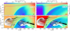 |
Fig. 1 Planck (panels a and b) and Rosseland (panels c and d) mean opacities. Panels a and c: maps of the temperature- and pressure-dependent gas mean opacities. The pink lines represent the dust mean opacities as functions of temperature. Panels b and d: final effective mean opacities, with the lime-coloured contour indicating the dust sublimation temperature, TS, for each pressure value. The white and black dots mark the temperaturepressure pairs that occur in our simulations, representing a snapshot of the quiescent and the outburst stage, respectively. |
2.3 Irradiation flux
The method used in our models to efficiently describe the frequency dependence of the stellar irradiation was based on Kuiper et al. (2010). In the following, we review the specific implementation of the method in our models. We hereby expand upon the description used by Sudarshan et al. (2026) by including the frequency-dependent gas opacities.
We calculated the total irradiation flux at every radius with (we refer to Appendix B for a derivation),
 (9)
(9)
with the stellar radius R*, the Stefan-Boltzmann constant σSB, the number of frequency bins n, the central frequency of a bin νi, its spectral weight wi and its radial optical depth τrad(νi, r). The effective stellar temperature T*,eff takes the contribution of accretion shock luminosity (following the description given in Appendix C) into account. The spectral region considered for the frequency-dependent opacities extended from 0.1 μm to 10 μm and was separated into 50 bins as a compromise between computational efficiency and accuracy. Since the absorption of irradiation is typically governed by the Planck means, we chose the direct averages within the frequency bins for the gas opacities. A visualisation of the binned frequency-dependent opacities for both gas and dust, in relation to the irradiating stellar spectrum, is given in Fig. 2. The temperatures of the displayed blackbody spectra include contributions from both the stellar and accretion shock luminosity. The colour coding of the bins corresponds to their relative spectral weight wi/max(wi). Following the definition of wi in Appendix B, the bin with the largest weight (i.e. carrying most of the energy) is located at the maximum of Bν(ν, T*,eff), which shifts only slightly under the influence of the maximum accretion luminosity. The wavelength range beyond 10 μm, which we did not consider in our irradiation description, only incorporates ~0.2% of the total irradiation energy and could therefore be neglected. The gas opacities are displayed for two different temperatures, with the density being kept constant. When considering the effect of the dust-to-gas mass ratio, the contribution of the gas to the total opacity can significantly exceed the impact of the dust, especially at small wavelengths and low temperatures.
Without frequency-dependent irradiation, we can set n = 1 and wi = w = 1 in Eq. (9), τrad(ν, r) becomes the total radial optical depth τrad(r), and we arrive at the usual expression for the grey irradiation flux,
 (10)
(10)
2.4 Viscosity
For most models in this work, we used the same description for the temperature-dependent viscous α parameter as in Paper I,
![Mathematical equation: \alpha=(\alpha_\mathrm{MRI}-\alpha_\mathrm{DZ}) \frac{1}{2} \left [1 - \mathrm{tanh}\left ( \frac{T_\mathrm{MRI}-T_\mathrm{g}}{T_\Delta}\right)\right]+\alpha_\mathrm{DZ} , \label{eq_alpha}](/articles/aa/full_html/2026/03/aa57408-25/aa57408-25-eq14.png) (11)
(11)
where αMRI and αDZ describe the viscosity of the MRI active and dead zone regions, respectively, and TMRI represents the threshold temperature around which the MRI becomes active. Following Flock et al. (2019) and Paper I and the motivations given therein, we set αMRI = 0.1, αDZ = 10−3 and TMRI = 900 K. While we implemented a narrow transition between αMRI and αDZ with a smoothing parameter TΔ = 25 K for the models in Paper I, we expanded the transition range for the new models of this work to TΔ = 70 K. The influence of this parameter, together with the effects of a lower value of αDZ, is investigated in Appendix D.
Previous studies have suggested that the effective viscosity does not respond instantaneously to changes in disc properties (e.g. Hirose et al. 2009; Flock et al. 2017; Ross et al. 2017; Held & Latter 2022). Instead, there might be a significant delay in α adapting to alterations of the thermal and ionisation structure. We analysed the effects of a delay like this by adapting Eq. (11) accordingly and by incorporating this description in additional models. We present the modelling procedure and its consequences in Appendix E.
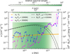 |
Fig. 2 Frequency-dependent gas and dust opacities in relation to the irradiating blackbody spectrum of the central star. The black lines indicate the Planck function of the irradiation, where the dash-dotted line represents the star during the quiescent phase (with negligible contribution from the accretion luminosity), whereas the dashed line shows the irradiating spectrum that includes the effect of the maximum accretion luminosity occurring in our models. The separation of the frequency space into the 50 bins is indicated by the thin vertical lines, where each bin is coloured according to its relative spectral weight. The orange crosses mark the dust opacities in their respective bins, multiplied by the maximum dust-to-gas mass ratio f0. The gas opacities in each bin were evaluated for a density of 10−10 g cm−3 and are shown for two representative temperatures: 1000 K (blue crosses) and 3000 K (magenta crosses). |
2.5 Numerical considerations
The majority of the numerical parameters and boundary conditions were directly adopted from Paper I. We briefly present the relevant differences.
To allow efficient radiative cooling, the vertical domain must be large enough to capture the transition from the optically thick disc to the optically thin atmosphere at every radius. Additionally, the polar boundary conditions should not inhibit the cooling process. In ensuring that, taking into account the new opacity descriptions of the models of this work, the polar domain was expanded to Nθ = 192 linearly spaced cells and covered a range in θ of π/2 ± 0.22, in contrast to π/2 ± 0.15 considered in our previous models. The radial domain remained separated into Nr = 2048 logarithmically spaced cells and extended from rin = 0.05 AU to rout = 10 AU. As a polar boundary condition for the temperature, we set
 (12)
(12)
which is very similar to the condition used in Paper I. We ensured that the resulting values are lower than the typical boundary temperatures in our models, enabling the disc to cool efficiently.
The sensitive temperature- and pressure-dependence of both the mean and frequency-dependent opacities necessitated the application of an under-relaxation scheme to the solver algorithm to maintain numerical stability. To exclude any impact on the onset and evolution of the episodic accretion events, the under-relaxation scheme was only applied in the optically thin disc atmosphere, where numerical instabilities are most prevalent. The detailed strategy and consequences of this method are explored in Appendix F.
3 Results
We conducted a multitude of 2D radiation hydrodynamic simulations with different combinations of the newly implemented physical effects. Table 2 lists the names and configurations of the various models presented in this section, including MREF* from Paper I as a reference. While the model DUST only considered the effects of the DIANA standard dust opacities for both the mean values and the frequency-dependent irradiation, NOFREQIRR combined the new descriptions for mean opacities of both the dust and the gas, but the irradiation was treated as frequency-integrated (i.e. grey irradiation), using the Planck means as absorption coefficients. The FULL model incorporated the new mean opacities and frequency-dependent irradiation, taking into account the contributions of both gas and dust. Additionally, the models DUST and FULL were simulated with and without the effect of accretion luminosity feedback. The values of the remaining physical and numerical parameters used in all simulations are listed in Table 3.
3.1 Effect of dust opacities
To isolate the effect of the new description of dust opacities using the DIANA standards, we analyse the initial outbursts in the models MREF* and DUST, starting from essentially the same initial hydrostatic structure. Figure 3 shows a comparison between these two models in the initial configuration, the outburst stage and the post-burst structure. The small difference in the gradient of the initial surface density profiles at the DZIE, recognisable in panel b, is due to the discrepancy between the values of TΔ of the two models. The vertical optical depths of the initial models shown in panel c reveal that the DIANA opacity description results in a higher optical thickness of the disc compared to the constant opacity values in MREF*. For instance, at a radius of 1 AU, τvert differs by a factor of 1.5 between DUST and MREF*. Since the surface density is equal outside a radius of ~0.2 AU, the heat produced by viscous accretion near the midplane can become trapped more efficiently in the case of DUST. This has a variety of consequences for the evolution of the TI cycle. Comparing the MRI activation fronts in panel a (black contours) reveals that a considerably larger portion of the dead zone is heated up and made MRI active in the DUST model. The heating front, launched after activating the MRI near the DZIE, is able to travel further outwards compared to the optically thinner disc in MREF*, where radiative cooling is more efficient. Consequently, the outermost density- and pressure bump emerging from the burst cycle (i.e. the peak in the surface density in the post-burst state) lies at a larger radius in the DUST model. Furthermore, the MRI active region becomes hotter, allowing for a larger fraction of the dust content to be sublimated. Hence, the upper equilibrium branch of the S-curve describing the instability cycle shifts to higher temperatures (as explored further in Sect. 4.3).
The magenta lines in panel a of Fig. 3 mark the τrad = 1 surfaces for the stellar irradiation. In the case of DUST, τrad has to be understood as the optical depth considering the total irradiation flux, τrad,tot. Hereby, τrad,tot = 1 was calculated as the radius at each height at which Firr(r) (Eq. (9)) has decreased to Firr(R★)e−1. The surface lies at larger heights compared to MREF*, which creates the drop in relative temperature between the two magenta lines because the stellar irradiation is absorbed sooner behind the dust sublimation front in DUST.
Another consequence of the higher dust opacities in DUST becomes discernible in the comparison of the post-burst states. Since the MRI can be kept active even at lower surface densities than in MREF*, the TI cycle in DUST not only engulfs a greater part of the dead zone, but also removes more mass from the affected regions. As a consequence, although the overall shape of the surface density profile in the post-burst state is the same in both models (including the positive gradient in the burst region), the absolute values of Σ in DUST are lower. Despite the lower surface density, the vertical optical depth in the post-burst state is still higher. This can be understood by considering that the minimum surface density necessary to keep the MRI active ( ) depends on the balance between heating and cooling efficiency, both of which depend on the surface density. In the DUST model, the more potent heat trapping near the midplane has to be compensated for by a greater diminishment of the surface density to enable effective cooling. However, a lower surface density also decreases the viscous heating efficiency, as a consequence of which, the equilibrium at
  allows for a larger vertical optical depth.
Sections 3.2 and 4.3 show that the evolution of the disc during burst cycles is mainly determined by the dust opacities, while the contribution of gas is only marginal. Therefore, the analysis of the onset, progression, and consequences of the outburst under the effect of the DIANA opacities was conducted in the context of the FULL model in the following sections.
Model names and configurations.
Model parameters.
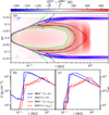 |
Fig. 3 Comparison between the models MREF* and DUST. Panel a: map of the temperature difference between the two models at a stage when the MRI active region has reached its largest extent during a burst. The black, green, and magenta contour lines represent the MRI transition, the dust sublimation front, and the τrad = 1 surface, respectively, where the dashed lines correspond to DUST and the solid lines to MREF*. Panels b and c: surface density and total vertical optical depth, respectively, of both models at two different stages: the initial hydrostatic structure (blue), and the state after the initial burst, when most of the density bumps have diffused (red). |
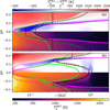 |
Fig. 4 Differences between the models DUST and FULL during quiescence (panel a) and outburst (panel b). The coloured contour lines represent the same transitions as in Fig. 3, with the solid lines corresponding to DUST and the dashed lines to FULL. The upper halves of the panels show the differences in temperature between the two models, while the lower halves depict the absolute temperature of DUST. |
3.2 Effect of gas opacities
The FULL model incorporates the mean and frequencydependent gas opacities, as calculated by Malygin et al. (2014), in addition to the DIANA standard dust opacities. We start the analysis of their combined effects by comparing FULL to the previously investigated DUST model. Figure 4 displays the discrepancies between these two configurations for both the quiescent (panel a) and the outburst phase (panel b). Additionally, the lower hemispheres of the two depicted snapshots show the temperature map of DUST. In both models, the accretion shock luminosity feedback is included.
The structure of the quiescent inner disc shows several remarkable differences. The temperature in the optically thin, gaseous atmosphere is significantly higher (by up to 2000 K) in the case of the FULL model. While we assumed a constant value of 10−3cm2g−1 for the irradiation and the Planck mean gas opacity in the DUST model, the corresponding opacities in FULL adapted freely to the conditions in the atmosphere, typically exceeding 0.1 cm2 g−1 (see Fig. 1), leading to a higher temperature in the equilibrium between heating and cooling. For the definition and evaluation of the equilibrium temperature, we refer to Appendix G and Sect. 3.4.
The shapes and positions of the MRI transition, the dust sublimation front, and the τrad,tot = 1 surface are strongly altered by the adaptive gas opacities. Due to the typically higher irradiation opacity of the FULL model compared to DUST, the stellar radiation is absorbed much sooner in the vicinity of the midplane, shifting the τrad,tot = 1 surface significantly closer towards the star. Consequently, the midplane temperature decreases below the dust sublimation and MRI activation thresholds much sooner, placing these transitions at the midplane at smaller radii as well. As a result, there is only a very small region (<0.015AU) at the disc midplane that can be considered to be dust-free, assuming that the magnetic truncation radius lies approximately at the inner boundary. This is the case even though we neglected the attenuation of the stellar irradiation between the stellar surface and our computational domain.
Similar to what we explored in Fig. 3, the region between the two τrad,tot = 1 surfaces is significantly cooler in the FULL model. At a height of z/r ~ ±0.1, the gaseous atmosphere is optically thin enough in both models such that the τrad,tot = 1 surfaces approximately coincide again outside of 0.2 AU, where the optical depth is mainly determined by the dust.
While the shapes of the transitional surfaces show a pointy feature at the midplane in the DUST model, they form a more rounded structure and become very shallow at a height of z/r ~ ±0.05 in the case of FULL. The MRI activation front and the inner dust rim become vertical just outside 0.2 AU in DUST, whereas they approach the polar boundaries only slowly in FULL, maintaining a hot, gaseous atmosphere at much larger radii.
Analogous to panel a of Fig. 3, panel b of Fig. 4 compares the structure of DUST and FULL at the respective times when the MRI active region has reached its greatest extent during an accretion event. The depicted outbursts are again part of the initial cycle, starting from the same hydrostatic initial model. The comparison of the MRI transitions (black contours) and dust sublimation fronts (green lines) indicates that the instability affects almost exactly the same region of the dead zone in both models, hinting at the dominance of the dust opacity, rather than the gas contribution, during the burst. Within the MRI active region near the midplane, the temperatures only start to diverge very close to the star, where the material becomes hot enough to sublimate the dust content to an extent at which the gas opacity (especially κR,g) becomes influential again. The similarities in the optically thick parts of the disc during the outburst, as well as the slight differences, manifest themselves in the shapes and positions of the S-curves, which are investigated further in Sect. 4.3.
In front of the inner dust rim, the τrad,tot = 1 lines differ between the two models, similar to what was observed in the quiescent phase. Due to the large amounts of material being accreted inwards during the outburst cycle, the midplane becomes optically thick enough to allow for the τrad,tot = 1 surfaces to reach the inner boundary in both models.
3.3 Temporal evolution of the outburst phase
As a next step in analysing the effect of the new opacity descriptions, we compared the structure and evolution of the MRI-activated TI burst cycle following the quiescent phase between the models FULL and MREF*. Figure 5 shows five snapshots in time illustrating the evolution of a complete outburst cycle. The top row presents the 2D temperature structure of FULL, analogous to that shown for MREF in Paper I, but on a logarithmic temperature scale. At t = tTI, the MRI is activated in the dead zone at the midplane, just outside the DZIE. The sudden increase in heating efficiency by viscous dissipation launches heating fronts into the dead zone, progressively activating the MRI. The front stalls when the surface density valley trailing it reaches  (at t = tc1), below which the MRI can no longer be sustained. It is then reflected into a cooling front that travels back towards the star, shutting down the MRI activity. This process repeats several times as smaller reflares (the first of which is ignited at t = trefl and expands until t = tc2) until enough material has drained from the inner disc onto the star to prevent further MRI activation in the dead zone. The quiescent phase is then re-established at t = tquies.
The second row of Fig. 5 depicts the corresponding surface densities and radial profiles of  for both the FULL and MREF* models. The first panel shows that at t = tTI, FULL requires less overall mass in the inner disc for the conditions of MRI activation to be fulfilled. The reason for this difference is twofold: On the one hand, the DZIE and, consequently, the location of the first MRI activation in the dead zone reside at smaller radii, where the viscous heat dissipation is more efficient (despite the different choice of TΔ, the effects of which are explored in Appendix D). On the other hand, the higher dust Rosseland mean opacities in the dead zone increase the effectiveness of heat trapping near the midplane, which also shifts the profile of
  to lower values. However, the slope of
  remains mostly unchanged. Remarkably, the combination of a less massive inner disc at t = t and the shift of
  results in the outermost density- and pressure bump produced by the TI cycle being placed at the same location (r ~ 0.7 AU) in both models.
At t = trefl, the density between the retreating cooling front and the star has to be much lower in the FULL model in order for the heating by irradiation to become dominant and stop the retreat of the cooling front. This inability for further cooling closer to the star ultimately leads to the reignition of the MRI behind the stalled cooling front and the development of the reflares. After each reflare has placed a density maximum within the inner dead zone, the surface density retains an overall increasing slope in the regions affected by the burst at the beginning of the quiescent phase.
The third row of Fig. 5 reveals that the aspect ratio is very similar in both models during the evolution of the outburst. In the regions where the equilibrium on the upper branch of the Scurve is established (see Sect. 4.3), H/r adopts a radial power law with an exponent of 0.48, as already recognised in Paper I. This relation is a consequence of the temperature on the upper branch being roughly constant with radius (with a small dependence on surface density, as discernible in the S-curve shown and analysed in Sect. 4.3). Following the definition of H, H/r ∝ T1/2r3/2r−1 ∝ r1/2, which is consistent with our finding. With this scaling, the aspect ratio at a radius of 0.5 AU can be increased by a factor of up to two during the burst phase.
A more detailed evolution of the surface densities, as well as the accretion rates of the models FULL and MREF*, is illustrated in Fig. 6. Comparing the space-time diagrams in panels a and c shows that while the individual flares occupy more time in the case of FULL, the duration of the entire burst cycle is approximately equal in both models. As investigated in Paper I, the pressure bump at the DZIE in the quiescent phase is destroyed by the TI cycle and re-established after the burst has ended. During the accretion event, multiple pressure bumps are placed throughout the inner disc by the individual flares. The new opacity description does not have any significant effect on the placement and evolution of these maxima.
Panel b of Fig. 6 displays the evolution of the accretion rates of both models over their entire simulation time, which includes the initial TI cycle, the quiescent phase in which the inner disc is refilled by accretion and the viscous evolution of the dead zone, and the subsequent outburst. For the FULL model, the simulation of the quiescent phase had to be partly interpolated between the burst cycles due to computation time restrictions. We lay out the details as well as the consequences for the timescales of the quiescent phases in Appendix H. It is expected, however, that the refilling of the material at the DZIE is slower in the FULL model due to the smaller extent and lower temperature of the MRI active region at the midplane in the quiescent phase compared to MREF* (and, equivalently, DUST, as shown in panel a of Fig. 4). As a consequence, the total amount of angular momentum being transported outwards and taken over by the material behind the DZIE is decreased as well, making the accumulation of mass in the inner dead zone less efficient and prolonging the quiescent phase.
Panel d provides a more resolved view of the accretion rates during the episodic accretion events occurring in both models. The times at which the snapshots shown in Fig. 5 were extracted are marked as vertical dotted lines for the example of FULL. As was already discernible in panels a and c, the duration of the individual flares is increased in FULL due to the necessity of more material having to be accreted onto the star in the case of an optically thicker disc. The larger diminishment of density between the cooling front and the star, explained above in the context of Fig. 5, manifests in panel d as the more pronounced dips in accretion rate between the reflares. Although the evolution of the accretion rates during the burst cycles differs between the two models, the maximum accretion rate is approximately the same, as is the total mass accreted onto the star with a value of ~10−5 M⊙.
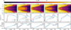 |
Fig. 5 Evolution of the outburst in the FULL model compared to MREF*. The different columns correspond to different evolutionary stages, starting from the ignition of the burst at t = tTI, chronologically proceeding through the burst stage and ending with the beginning of the next quiescent state at t = tquies. The top row shows the temperature maps of FULL with the black and green contour lines marking the MRI-transition and the dust sublimation front. The middle row depicts the surface densities for both MREF* and FULL at the same stages during their respective evolution. The vertical dotted lines in the first panel indicate the locations of the DZIE in the corresponding model of the same colour. The panels in the second, third, and fourth column also show the respective profiles of |

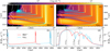 |
Fig. 6 Evolution of the surface densities and accretion rates. Panels a and c: space-time diagrams of MREF* and FULL, respectively. The displayed time spans have the same length. The white contours mark the positions of local pressure maxima, while the cyan line indicates the DZIE at the midplane. Panel b: accretion rates for both models over their entire simulation times. The dashed section of the blue line represents the interpolation between the two bursts. Panel d: magnification of the burst occurring in FULL. The vertical dashed lines mark the time of the ignition of the outburst (tTI), the first and second reflections of the heating front (tc1, tc2), the launching of the first reflare (trefl) and the beginning of the quiescent phase (tquies) for FULL. For comparison, the accretion rate resulting from the burst in MREF* is overplotted, shifted in time so that the respective tTI for both models align. |
3.4 Effect of frequency-dependent irradiation and manifestation of the equilibrium temperature degeneracy
Figure 4 and the top row of Fig. 5 include a remarkable detail inherent to the FULL model: a sudden drop in temperature, especially noticeable in the disc atmosphere near the polar boundaries, that does not necessarily coincide with either of the transitions marked in the figures. Intuitively, it stands to reason that this feature might be a consequence of either the effects of frequency-dependent irradiation or the transition to an opacity dominated by dust. In order to show that this temperature drop is an inherent property of the gas Planck mean opacities, we compare the quiescent structure of FULL to the NOFREQIRR model in which we only consider the Planck mean opacities for the absorption of the irradiation flux. We aim to confront the temperature structures resulting from our numerical calculations with the expected equilibrium temperature Teq of the optically thin medium in both models. A derivation of the analytic expression for Teq is presented in Appendix G.
The effect of frequency-dependent irradiation is illustrated in panels a and c of Fig. 7. While the midplane of the inner disc is largely unaffected, the 2D temperature structure is altered significantly. In the FULL model shown in panel a, the hot, gaseous atmosphere reaches higher temperatures close to the star and extends to much larger radii when compared to the temperature map of NOFREQIRR displayed in panel c. However, the temperature drop is still manifested in NOFREQIRR, indicating already that its presence is not a consequence of frequency-dependent irradiation. The shape of the dust sublimation front (green contour) is affected as well by the altered position of the temperature jump. Additionally, the vertical temperature profile in the cool regions is more smoothed-out in FULL, in contrast to the very noticeable transition from the optically thick disc to the warmer atmosphere in NOFREQIRR.
Figure 7 also analyses the origin of the temperature jump, which effectively separates the inner disc into a low and high temperature regimes. To efficiently calculate the analytic equilibrium temperature for comparison to the numerical values, we define the function f (r, Tg, Pg) on the basis of Eq. (G.3),
 (13)
(13)
The roots of f (r, Tg, Pg) represent the solutions for Teq. Panels a and c of Fig. 7 compare the radial profiles of the temperatures of the underlying models at a height of z/r = 0.2 (to ensure optical thinness) with the analytic equilibrium solution. We applied a root finding algorithm of the secant method to solve f (r, Tg, Pg) = 0 at every radius. In order to isolate the consequences of the gas mean opacities, we excluded the effect of dust (fD2G = 0), the varying profile of the gas pressure (Pg = const.), and the attenuation of the irradiation (τrad(νi, r) = 0) in the calculation of Teq. For the constant Pg, we chose the mean value at z/r = 0.2 of 6 ∙ 10−7 dyn cm−2. A full evaluation of Teq with all contributions included in Eq. (G.3) is demonstrated in Appendix F.
The temperature profiles of our numerical models fit the analytic solution reasonably well in both the FULL and the NOFREQIRR models, considering the neglected effects described above in the analytic calculations. Most notably, the presence and location of the temperature jump can be exactly recreated in both models by the simplified analytic considerations. For further analysis, panels b and d show f (r, Tg, Pg) as a function of Tg for four different radii, respectively, calculated with the same simplifications as indicated above. The gold lines depict f (r, Tg, Pg) at a radius just before the location of the temperature jump. In this case, the only available solution for the equilibrium temperature is in the high-temperature regime. The blue curves were calculated at a larger radius where a second root becomes available, which is the solution adopted by our numerical solver algorithm. Starting from the blue profile, f (r, Tg, Pg) allows for three solutions until the radius of the purple curve, after which only one solution for Teq is allowed again. Consequently, for radii between the blue and the purple curves, the solution for the equilibrium temperature is degenerate. This phenomenon is equivalent to the equilibrium temperature degeneracy described by Malygin et al. (2014).
The star markers indicate that our models immediately switch to the low-temperature solution as soon as it becomes available and do not revert to the high-temperature regime at larger radii. Arguably, this is a consequence of our chosen method of setting up the initial model. Since we start from a cool disc and let the temperature increase by radiative transport, the low-temperature solutions are conserved. Conversely, if we chose to start from a hot disc and let it cool down radiatively towards the initial model, the temperature jump would occur just before reaching the radius of the purple curves. As argued by Malygin et al. (2014), the available intermediate solutions are always unstable and will therefore not be adopted by our solver algorithm. This is the reason for the visible gap in panels b and d of Fig. 1 in the coverage of the temperature-pressure pairs occurring in our simulations. Regardless of the choice of the initial model creation, the temperature jump intrinsically has to manifest at a radial range bounded by the blue and purple curves shown in panels b and c of Fig. 7 in all models that include the gas mean opacities of Malygin et al. (2014).
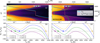 |
Fig. 7 Temperature jump as a consequence of the equilibrium temperature degeneracy. Panels a and c: temperature maps of the quiescent phase for the models FULL and NOFREQIRR, respectively. The dashed red lines show the radial profiles of the temperatures at a height of z/r = 0.2 (indicated by the dotted white line). The solution of Eq. (G.3) for Teq at every radius is represented by the blue line. The green contours mark the dust sublimation fronts. Panels b and d: function given in Eq. (13), evaluated at four different radii for both models, respectively. The star-shaped markers indicate which of the available solutions is adopted by the solver at each radius. The same markers were used to locate the respective evaluation radii in panels a and c. |
3.5 Locations of radial and vertical τ = 1 surfaces
The availability of frequency-dependent opacities for both gas and dust enabled us to calculate optical depths at different wavelengths. Figure 8 presents the profiles of the radial (τrad(ν), panels c and d) and vertical (τvert(ν), panels a and b) τ = 1 surfaces for selected wavelengths in the upper hemisphere of the FULL model, including accretion shock luminosity feedback. Both the quiescent (panels a and c) and outburst phases (panels b and d) are represented.
For the τvert(v) = 1 surfaces, the optical depth was integrated along the (Cartesian) z-direction, starting from the upper polar boundary down towards the midplane. The positions of the surfaces for the different wavelengths can be understood by comparing them to the wavelength-dependent opacities shown in Fig. 2. At smaller wavelengths, radiation is more readily absorbed, especially due to the higher gas opacities. Remarkably, the disc can become optically thick even without the contribution of dust at the shortest wavelengths. Starting from about 1 μm and going to longer wavelengths, the surfaces lie deep within the disc at approximately the same position (for clarity, only τvert(1 μm) = 1 is shown). During a burst (panel b), the MRI active region inflates the disc significantly, pushing all τvert(ν) = 1 surfaces to greater heights. The effect of accretion luminosity feedback is clearly evident in the higher temperatures in the atmosphere near the star. However, its effect on the dynamics and position of the τvert(ν) = 1 lines remains mostly marginal. A small effect of the higher irradiation flux is the disturbance of the temperature jump caused by the equilibrium temperature degeneracy analysed in Sect. 3.4. The effective increase in stellar temperature slightly shifts the temperature jump to larger radii. After the burst phase, these new equilibrium solutions remain conserved (as also evident in comparing the first and last panels in the first row of Fig. 5).
In panels c and d, the τrad(ν) = 1 were calculated for the central wavelengths of a number of selected frequency bins. Generally, radiation in wavelength bins with high spectral weight can penetrate deeper into the disc, while radiation at small wavelengths is already mostly absorbed by the gas before reaching the dust sublimation front. As a consequence, the transition between optically thin and thick, considering the total stellar irradiation flux, τrad,tot = 1, lies deeper within the disc as well. Similar to the case for the τvert(ν) = 1 lines, the τrad(ν) = 1 surfaces are shifted away from the midplane during the outburst phase. Consequently, the surfaces become horizontal in the region beyond the MRI active zone up to several AU, indicating the shadowing effect of the puffed-up, hot inner disc.
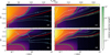 |
Fig. 8 Different τ = 1 lines for a disc in quiescence (panels a and c) and in outburst (panels b and d) shown atop the underlying temperature structure for the model FULL. In panels a and b, the dashed blue lines mark the τvert(ν) = 1 surfaces for different wavelengths, which are indicated in the labels in units of μm. The dashed lines in panels c and d show the locations of the τrad(ν) = 1 transitions for the stellar irradiation for several representative wavelength bins with the respective central wavelengths in μm marked in the labels. The colour of the dashed lines indicates the relative spectral weight of the bin. Additionally, each panel includes the dust sublimation front as the green line and the τrad,tot = 1 line for the total radial optical depth in red. |
3.6 Stability of burst features
The emergence of steep density features during a burst cycle (e.g. middle row of Fig. 5) raises questions about their dynamic stability. We emphasise that the RWI cannot be manifested in our axisymmetric models. For the analysis of the stability of the DZIE and the burst features, we relied on criteria that assess the linear RWI. A complete investigation of this aspect of the inner disc evolution, including non-linear effects, would require non-axisymmetric simulations, ideally, in 3D. Figure 9 shows an analysis of the density bumps that develop during the burst in the FULL model with respect to a potential Rossby wave and Rayleigh instability. In this context, we considered the Lovelace criterion (Lovelace et al. 1999; Lovelace & Romanova 2014) as a necessary condition for RWI, the halfway-to-Rayleigh limit (Chang & Youdin 2024) as a sufficient criterion, and the condition resulting from the fit to the amplitude of marginally stable features according to Ono et al. (2016) for comparison.
For the Lovelace criterion to be fulfilled, extrema in the vortensity profile q of the disc have to be present, while the halfway-to-Rayleigh condition is given as  −0.6, with κef the epicyclic frequency. In order to compare the density bumps occurring in our models with the descriptions of marginally stable features given in Table 2 of Ono et al. (2016), we approximated them by Gaussian bumps with corresponding amplitudes and widths. For the definitions of the relevant quantities for the three considered criteria, we refer to Appendix I.
The first expansion of the heating front during the accretion event occurring in the FULL model is analysed in the top three panels of Fig. 9. At t = tTI, no extrema in the vorten-sity profile are present. Even the DZIE does not fulfil any of the three criteria. If the density contrast at the DZIE increased further, the RWI might still become active. However, this is prevented by the emergence of the accretion event. The density peak travelling outwards alongside the heating front produces sharp minima in both the vortensity and  profiles, fulfilling both the Lovalace and halfway-to-Rayleigh criteria. Since
  becomes negative, these features can even be considered to be Rayleigh unstable. After the heating front has stalled, Rayleigh stability is quickly restored and the density feature starts to diffuse on the viscous timescale. A part of this process is shown in the bottom three panels of Fig. 9. The time between the density feature reaching its outermost position and the transition to stability according to the upper limit of the halfway-to-Rayleigh criterion (orange line) is around seven years, which corresponds to ~12 local orbits at the central radius of the bump. During this time period, the amplitude of the feature is large enough to also render it unstable according to the criterion proposed by Ono et al. (2016). Regarding this condition, the RWI remains even after the halfway-to-Rayleigh threshold is crossed. However, the width of the density bump is always larger than the local scale height, which should make the halfway-to-Rayleigh criterion more accurately applicable in this time frame (Chang & Youdin 2024).
By the time the burst cycle has completed (at t = tquies), the vortensity profile still shows minima at the locations of the density bumps. However, the inner disc is stable to the RWI throughout its entire extent according to both the halfway-to-Rayleigh and Ono et al. (2016) criteria.
Although these conditions should not directly be influenced by the levels of turbulence (Lin 2013), the steepness of the density structure at the DZIE and the evolutionary timescale of the features placed within the dead zone are subject to the description of the viscous α parameter. An investigation of the effect of a lower value of αDZ and a sharper transition at the DZIE on the RWI of the inner disc is presented in Appendix D.
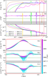 |
Fig. 9 Analysis of the stability criteria for the density maxima generated during the outburst in the FULL model. Top three panels: temporal evolution of the surface density Σ (panel a), the parameter κ2/Ω2 (panel b), and the vortensity q (panel c). These are shown as snapshots during the time frame starting from the ignition of the burst (t = tTI, blue line) until the first density bump has reached its outermost position and κ2/Ω2 becomes positive (brown line). Additionally, the pink line represents the disc at t = tquies. The dashed green line in panels b and (b1) indicates the halfway-to-Rayleigh stability threshold. Bottom three panels: Same three quantities, but zoomed into the radial region where the first density bump is located. The colour-coded time frame begins at the moment when min(κ2/Ω2) > 0 and includes the transition from instability to stability according to the halfway-to-Rayleigh criterion, reached at t = 3877.7 yr (orange line in panels a1, b1, and c1 and in the colour bar). Quantities in panel b, (b1), panel c, and (c1) are depicted on a logarithmic scale with a linear transition around zero, indicated by the grey shaded region. |
4 Discussion
The models analysed in this work show that although the thermal structure of the inner disc is crucially affected by the careful treatment of dust and gas opacities, the periodic instability mechanism disrupting the inner disc and leading to accretion outbursts is operational in all cases, and hence denotes a robust feature of disc evolution. In this section we discuss the potential observational prospects expected from our simulations and address the possible consequences of the RWI and Rayleigh instability of burst features. We further analyse the dominance of the dust opacities during the burst evolution, indicated by our results, by investigating the S-curves of different models. Finally, we assess the importance of considering detailed dust and gas opacities for our understanding of the inner disc structure and its evolution before describing the limitations of our models.
4.1 Preview of potential observational consequences
The significant changes in the temperature structure of the inner disc resulting from our treatment of the gas opacities might have considerable implications for the observational signatures produced. While a more detailed analysis will be part of future work, we aim to provide a first estimate of the expected observational effects in this section.
Concerning the spectral energy distribution (SED), we expect a higher flux in the near-infrared from the hot gas atmosphere, which fills the spectral region in which dust does not contribute due to sublimation. In the mid- to far-infrared, changes in the SED may be insignificant, as these regions are primarily dominated by dust emission. The implementation of temperature- and density-dependent gas opacities in radiative transfer codes, such as RADMC-3D (Dullemond et al. 2012), is non-trivial and warrants a dedicated study. To still assess the influence of the altered inner disc structure by the new opacity descriptions on the resulting SEDs, we adopted a simplified approach in the following.
Instead of determining the absolute values of the SEDs, we only intend to estimate the differences in the emissions of the MREF* and FULL models by calculating
 (14)
(14)
where the frequency-dependent flux is evaluated for each model with (Chiang & Goldreich 1997).
 (15)
(15)
with z being the cylindrical height and k a constant factor that is cancelled when evaluating Eq. (14). For the calculation of τvert(ν, r, z), we took the contributions of both the dust and gas opacities into account. This method assumes that both the gas and dust components are radiating as blackbodies at their respective local temperatures.
Figure 10 shows the results of Eq. (14) for both the quiescent and outburst phases in the near- to mid-infrared spectral region, with markings for the main infrared bands. The flux in the nearinfrared is significantly enhanced in the FULL model compared to MREF by virtue of the hotter disc atmosphere. Starting from the M-band, the flux in MREF is slightly increasing above the flux emerging from FULL due to the less massive inner disc in FULL and the rise in influence of the dust opacities at larger wavelengths. The differences between the quiescent and outburst phases are only marginal, with the dominance of the FULL model shifting slightly towards the mid-infrared region. This simplified approach presents a first idea of the significance of the change in the structure of the inner disc by considering (primarily) the detailed gas opacities on the spectral emissions. However, to determine the precise shape of the SEDs resulting from our models, dedicated radiative transfer calculations with careful implementation of the gas opacities and, ideally, thermochemical considerations in the hot disc corona are necessary.
Apart from effects on the SEDs, the hot gas in the disc atmosphere might lead to the emergence of several line emissions. For instance, CO overtone emissions have previously been associated with a hot gas component with temperatures of 3500 K in the innermost regions of Class I discs (Lee et al. 2016; Rudy et al. 2023). This temperature regime might be reached in our models in the thin disc atmosphere (e.g. Fig. 8).
The disc regions close to the τrad,tot = 1 surface with temperatures in the range of 1500-3000 K could fulfil the conditions for producing H2 rovibrational line emission in the NIR by collisional excitation in the dense, hot gas (Beck & Bary 2019). Furthermore, the hot, thin gas atmosphere may also enable forbidden line emissions, particularly of [OI], which, for instance, has been observed to originate from the inner regions within the disc of ET Cha (Woitke et al. 2011). However, forbidden line emissions are typically also expected to be produced in jets and winds emerging from the inner disc (e.g. Flores-Rivera et al. 2023). The true origin might be discernible by disentangling different velocity components of the lines.
The high-resolution spectrum of the frequency-dependent gas opacities calculated by Malygin et al. (2014) might allow us to track the strength and origin of specific line emissions in the near- and mid-infrared, as would be observable by instruments such as NIRSpec or MIRI of the James Webb Space Telescope. A detailed investigation of the implications for the SEDs and the line emission spectra using tools for radiative transfer modelling, such as RADMC-3D, goes beyond the scope of this study and is left for future work.
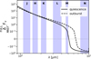 |
Fig. 10 Differences in the SEDs between the MREF* and FULL models during the quiescent and outburst phases. The shaded areas mark the wavelength regions covered by the various infrared bands. |
4.2 Possible implications of the instability of density features
As shown in Sect. 3.6, the density spikes travelling outwards alongside the expanding MRI active region are prone to the Rayleigh instability, while the bumps left behind in the inner disc continue to fulfil the conditions for RWI for more than ten local orbits. The RWI has been recognised as an effective production mechanism for vortices at the edges of planetary gaps (e.g. Li et al. 2005; Hammer et al. 2019; Ziampras et al. 2025b) or at strong transitions in turbulence, such as the edges of dead zones (e.g. Faure et al. 2014; Flock et al. 2015; Roberts et al. 2025). The duration of the linear growth phase of the RWI is on the order of ten local orbits, after which vortices are readily formed (Lyra & Low 2012; Bae et al. 2015). However, this mechanism is intrinsically non-axisymmetric and does not manifest in our models. Based on the analysed RWI criteria and the timescales of linear growth and saturation of the instability, we conclude that the density bumps placed by the outburst mechanism, including its reflares, might lead to the emergence of vortices in a non-axisymmetric geometry. However, these vortices typically merge together quickly to form a single vortex (e.g. Bae et al. 2015) and can decay on short timescales due to processes such as viscous diffusion (governed by αDZ), slow cooling or dust dynamics (Rometsch et al. 2021; Ziampras et al. 2025a,b). Vortices produced by RWI at the edges of dead zones might survive longer (Regály et al. 2017), but the results of our work indicate that the DZIE seems to be mostly stable. Therefore, we expect the vortices resulting from RWI in the density bumps to decay on a short timescale while new vortices are continuously produced by the ongoing burst mechanism. A lower value of αDZ might allow the vortices to linger in the dead zone for a longer time.
Rayleigh instability of density features effectively results in their radial diffusion on a dynamic timescale (e.g. Yang & Menou 2010). Since the formation of vortices would also effectively smooth out sharp density features, it is reasonable to assume that the bumps placed in the inner disc by the burst mechanism are not as pronounced as our models predict (Fig. 5).
The question remains of whether the Rayleigh or Rossby wave unstable, outward-moving density spikes pose an impediment to the expansion of the heating front. The progression of the heating front relies in part on the activation of the MRI by increasing the density ahead of the front above a critical value. Consequently, if the timescale of the dispersion of the density spikes by the instabilities is comparable to the timescale of the expansion of the MRI active region, the heating front may be slowed down and could possibly be stalled sooner. However, neither the possible impediment of the heating front nor the quicker dispersion of the density bumps will significantly affect the emergence of the burst cycles and the resulting density structure within the quiescent phase. Non-axisymmetric simulations are needed to investigate the interplay between these different instability dynamics in more detail.
4.3 Alteration of S-curves
A major part of Paper I revolved around the tracing of the episodic accretion events along S-curves of thermal stability. Panel a of Fig. 11 illustrates the effect of the new opacity descriptions on the shapes and positions of the curves in the Tg,mid-∑ plane. The S-curves are shown for the MREF*, DUST, and FULL models, calculated at a radius of 0.2 AU. They include the first flare of the burst cycle4, omitting the reflares for clarity.
The discrepancies between the MREF* and FULL curve are another manifestation of what we described in Sects. 3.1-3.3. In FULL, the TI is initiated at lower surface densities, the temperature in the MRI active region (high-state upper branch of the S-curve) is higher, and  lies at lower values. As described in Paper I and also discussed in other studies (e.g. Woitke et al. 2024), the upper branch of the S-curve is shaped by a thermostat effect. Thereby, a continuous rise in temperature is prevented by the sublimation of dust, allowing the increased radiative cooling to counteract the viscous heat dissipation and establishing the high-state equilibrium. The slopes of the upper branches only change at temperatures well below the dust sublimation threshold, where the dust-to-gas mass ratio is constant.
Curiously, the curves for DUST and FULL overlap exactly at the chosen radius. The underlying reason has already been mentioned in the context of Fig. 4. In the optically thick MRI active region, the radiative cooling is determined by the Rosseland mean opacities, which is always dominated by the dust contribution as long as a sufficient amount of dust is still present (see Fig. 1). Since this is the case at 0.2 AU, the gas opacities do not affect the S-curve at this location. They only become relevant when the temperatures reach values high enough for the majority of the dust to be sublimated, such that the values of κR,g and fD2GκR,d become comparable. This effect is revealed when calculating the S-curves closer to the star, where heating becomes more efficient. Panel a of Fig. 11 includes the upper branches of DUST and FULL at r = 0.08 AU, showing that they indeed start to diverge at high temperatures. The same effect would manifest even at larger radii if the disc were chosen to be more massive.
Along the lower branches, the discs evolve slowly on the viscous timescale, tν = r2/ν, determined by αDZ. Panel b of Fig. 11 shows the evolution of the surface density during the quiescent phase of the FULL model. It illustrates the refilling of the inner disc by accretion of material from larger radii and the diffusion of the density bumps produced by the previous accretion event. If no further burst cycles were to occur, the refilling would proceed until a hydrostatic, steady-state solution is reached, an estimate of which is shown as the dashed yellow line. However, the conditions for TI are fulfilled at t = tTI and the surface density structure is reset by the burst to approximately what is shown in panel b at t = tquies.
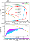 |
Fig. 11 S-curve behaviour with respect to the MRI-activated TI and evolution of the inner disc during quiescence. Panel a: S-curves of MREF*, DUST, and FULL, extracted from the respective quiescent phases (for MREF* and FULL) compared with the main flares of the accretion events (for all three models) at a radius of 0.2 AU. The arrows along the curves indicate the direction of evolution. The dashed black lines mark the critical values of the surface densities at which the respective upper branches end. The panel also includes the upper branches of the S-curves for the DUST and FULL models at r = 0.08 AU. Panel b: evolution of the surface density during the quiescent phase of FULL. The dashed yellow line is the approximate profile of the hydrostatic structure the disc would adopt if no TI were to occur. |
4.4 The necessity of including detailed opacity descriptions
Section 3 provides comparisons of simulations with different opacity descriptions. The confrontation of these models with each other allows us to gauge the necessity of complex and computationally expensive opacity descriptions for different use cases.
Sections 3.1−3.3 and 4.3 make clear that the evolution and extent of the episodic accretion event caused by MRI activation in the dead zone is only influenced by the mean dust opacity description, while the gas opacities and the frequency dependence of the irradiation do not play a major role. However, the position of the DZIE, and consequently, the location of the ignition of the outburst and the efficiency of the density pile-up during quiescence, is strongly affected by the gas contribution. Therefore, it cannot be assumed that the duration of the quiescent phase and the shape of the disc at t = tTI are independent of the gas opacities. Furthermore, as indicated in Sect. 4.3, for more massive discs and stronger viscous heating during the burst, the gas mean opacities could become the dominant contributor to the cooling efficiency if dust is sufficiently sublimated. Therefore, concerning the burst mechanism investigated in this work and Paper I, we propose that if the duration of the quiescent phase and the structure of the inner disc at the ignition of the TI are of interest, the gas mean opacities should not be neglected. For the burst phase itself, the careful treatment of just the mean dust opacities should suffice, but only as long as the thermostat effect on the upper branch of the S-curve can be sustained throughout the majority of the burst region.
The axisymmetric temperature structure of the inner disc is strongly affected by the gas opacities. As displayed in Fig. 4, the temperature in the disc atmosphere increases drastically when gas opacities are properly accounted for. The frequencydependent irradiation exacerbates this behaviour even further (Fig. 7). The radial temperature profile in the very inner disc in the vicinity of the midplane is strongly affected as well. While in the simpler MREF* model, the dust sublimation front is located outside 0.1 AU, it shifts to smaller radii (0.06-0.07 AU) in the FULL model, which agrees better with recent estimates of inner dust wall locations in discs around classical T Tauri stars (Pittman et al. 2022). Furthermore, the gas mean opacities evoke the manifestation of the equilibrium temperature degeneracy as a sharp jump in temperature, as analysed in Fig. 7. The location of the transition between the high- and low-temperature regimes is significantly affected by frequency-dependent irradiation. Additionally, determining the positions of different τ = 1 surfaces using frequency-dependent opacities allows us to gauge where observed radiation of different wavelengths originates. Therefore, for investigating the 2D temperature structure of the inner disc and analysing its observational consequences, gas opacities with both their mean and frequency-dependent values are of significant importance.
However, it is worth noting that including detailed opacity descriptions in simulations can entail considerable computational costs. Considering that the gas opacities depend on temperature and pressure in both their mean and frequencydependent versions, the necessary interpolations in each cell for each frequency bin can severely increase the computational load. For instance, all aspects of the computational setup being equal, the computational time for the FULL model was larger by a factor of around 2.4 in comparison to MREF*.
4.5 Model limitations
A major part of the limitations of the models of Paper I has been addressed in this work. However, several physical factors that may have an influence on our results were not taken into account.
In the equation of state (Eq. (8)), we assumed a constant value for μg of 2.35 for a mixture of hydrogen and helium with solar abundance, following Flock et al. (2019). The same assumption was used for fixing the first adiabatic index γ. However, μg and γ typically depend on the ionisation state of the material in addition to the chemical composition (e.g. D’Angelo & Bodenheimer 2013). While our assumption may still be reasonable for models with maximum temperatures around the dust sublimation limit (as in MREF*), it breaks down in the hot gaseous regions occurring in simulations with detailed gas opacities. In our models, the absorbed energy in the thin atmosphere translates directly into an increase in temperature, rather than being also invested in the partial ionisation of the gas at high temperatures. Additionally, energy may be expended for the endothermic process of H2 dissociation at temperatures higher than 2000 K. These simplifications could result in an overestimation of the temperatures in the atmospheres of the FULL and NOFREQIRR models. However, the ionisation state and its effect on the equation of state were taken into account in the calculations of the gas opacities by Malygin et al. (2014).
In addition to alterations in the equation of state in the thin, irradiated disc atmosphere, several important heating and cooling processes in this region were not captured by our radiative transport scheme. The optical thinness and consequential rarity of collisions result in weak coupling between the radiation field and the gas, leading to the prevalence of non-local thermodynamic equilibrium effects. In those cases, line cooling by atoms, ions and molecules can dominate the cooling process (Woitke et al. 2009; Sellek et al. 2024). On the other hand, photodissociation by the stellar irradiation can destroy relevant coolants, while photoionisation, photoelectric effects and absorption of ultraviolet radiation by, for instance, polycyclic aromatic hydrocarbons can significantly contribute to heating of the optically thin gas (e.g. Woitke et al. 2009; Wang & Goodman 2017). Additionally, gas and dust temperatures tend to decouple in the upper layers of the disc, warranting a more detailed treatment of the energetic exchanges between the radiation field, the dust and the gas component (e.g. Muley et al. 2023). Since the self-consistent thermochemical modelling exceeds the intentions of this work, the temperatures achieved in the thin irradiated disc atmosphere in our models should be regarded as approximate. The consideration of chemical processes in the thin gas and dust components, as performed by codes like GGchem (Woitke et al. 2018) or PRIZMO (Grassi et al. 2020) and implemented in hydrostatic disc structure models like ProDiMo (Woitke et al. 2009), in combination with the hydrodynamic evolution presented in our work, would result in a more complete picture of the thermodynamics of the inner disc.
As was the case for Paper I, the consideration of non-ideal magnetohydrodynamic (MHD) effects might change the evolution of the inner disc. For instance, Iwasaki et al. (2024) conclude that the region around the DZIE incorporates a transition zone, in which the radial mass transport is halted, effectively leading to an accumulation of mass, similar to the refilling of the inner disc shown in panel b of Fig. 11. Other works by Latter & Balbus (2012) and Faure et al. (2014) do not find a limit-cycle behaviour similar to our results in their MHD considerations of the dynamics of the DZIE. Consequently, the structure found in their models is prone to RWI (Faure et al. 2015; Roberts et al. 2025). Additionally, Roberts et al. (2025) find that the dead zone features a particular magnetic field topology as a result of magnetic flux transport near the DZIE. This field could possibly account for radial mass transport in the inner dead zone by driving a magnetic wind. Although a self-consistent treatment of non-ideal MHD in combination with the set-up of our work is computationally challenging, a reasonable compromise could consist of determining the MRI activity based on large-scale magnetic field structures, such as determined, for instance, by Steiner et al. (2025), in combination with tabulated values of ambipolar and ohmic diffusivities, as calculated in works of Desch & Turner (2015) or Williams & Mohanty (2025).
The values of the physical and numerical parameters entering our simulations (Table 3) were chosen for consistency with previous work and were motivated by observational and theoretical literature. Different choices of parameter values can affect the details of our simulation results, especially concerning the timescales of the quiescent and outburst phases. For instance, previous studies have indicated that the location of the inner boundary rin can affect the magnitude of accretion events caused by TI to a significant extent (Steiner et al. 2021 ; Elbakyan et al. 2025). However, since the main focus of this work is the effect of opacity descriptions, detailed further parameter and resolution studies go beyond the intention of our investigations.
The calculations of the gas opacities by Malygin et al. (2014) considered a wide range of atomic and molecular lines. Recent investigations of gas mean opacities use slightly different line lists and treatments of the line pressure broadening (Marigo et al. 2024). This can lead to discrepancies between the different approaches, especially in the low-temperature regime. However, we do not expect these differences to significantly affect the qualitative results of this study.
The equilibrium state during quiescence, especially in the vicinity of the DZIE, is considerably delicate. Small disturbances in the density or thermal structure, such as planet-disc interactions, vortices, gravitational disturbances or changes in the effective stellar luminosity, can launch the burst cycle far sooner than our models predict. Since such disturbances are not included in our models, the state of the disc at t = tTI, as displayed in the first column of Fig. 5, has to be understood as the latest possible quiescent structure. Non-axisymmetric 2D or 3D models, allowing for the emergence and evolution of vortices or gravitationally bound clumps, as well as consideration of embedded planets or interaction with the stellar environment, could reveal different timescales of quiescence between burst cycles.
5 Conclusion
The models we presented greatly expand on previously published results for the structure and radiation hydrodynamic evolution of the inner region of protoplanetary discs that include the inner permanently MRI-active region, the dust sublimation front, and the transition to the dead zone. We investigated the effect of detailed frequency-dependent and mean opacity descriptions for gas and dust on the 2D thermal structure of the inner disc and the emergence, evolution, and consequences of periodic accretion burst cycles caused by the activation of the MRI in the inner regions of the dead zone. Additionally, we included the stellar accretion shock luminosity and analysed the stability of features produced by the burst cycles with respect to the Rossby wave and Rayleigh instability. We summarise the main results below:
The consideration of the gas opacities as calculated by Malygin et al. (2014) significantly affects the structure of the inner disc. The dust sublimation front and the DZIE at the midplane are closer to the star than previously predicted. Consequently, the inner MRI active region during quiescent phases is restricted to smaller radii;
In the FLD approximation of radiative transport, the gas opacities additionally lead to a significantly higher equilibrium temperature in the optically thin gaseous regions;
The equilibrium temperature degeneracy, inherent to the gas mean opacities, manifests itself as a sharp temperature transition, effectively separating the thermal structure of the disc into a high- and low-temperature regime and shaping the vertical structure of the MRI transition and dust sublimation front;
The inclusion of the frequency dependence of the gas opacities in the irradiation shifts the equilibrium temperature transition and adds substructure to the thermal state of the inner disc, especially in front of the inner dust rim;
The dust-free regions can already become optically thick through the effect of gas opacities, especially at small wavelengths (<0.5 μm);
The mechanism leading to accretion burst cycles by activation of the MRI behind the DZIE is still functional in different treatments of opacity descriptions;
The effect of the gas opacities determines the initial conditions for the accretion outburst by setting the location of the DZIE. However, the thermodynamic evolution of the burst cycle itself is mainly determined by the Rosseland mean opacities of the dust. The equilibrium temperature in the viscously heated burst region on the upper branch of the S-curve is governed by a thermostat effect, where the decrease in optical thickness by sublimation of dust balances the enhanced heating by viscous energy dissipation. Only when the dust is (close to) being completely sublimated in regions with strong viscous heating do the gas opacities start to dominate the radiative cooling;
Higher dust opacities lead to lower values of the critical surface densities
 and
and  . As a consequence, the burst cycle can be initiated in less massive inner discs. However, the maximum accretion rate and total mass accreted during the burst remain independent of the opacity description;
The density spikes travelling outwards alongside the expanding MRI active region during burst cycles fulfil the conditions of the Rayleigh and Rossby wave instability. The viscously evolving density and pressure bumps placed in the inner disc by the burst can remain prone to RWI long enough to produce vortices in non-axisymmetric settings;
The burst cycles reset the density structure at the DZIE before the linear criteria for RWI are fulfilled, which might keep the DZIE stable during quiescent phases.
Our study highlighted the importance of considering detailed opacity descriptions, especially for the gas, in the inner regions of protoplanetary discs where temperatures become high enough to sublimate dust. Depending on the physical processes or structures of interest, a careful treatment of gas opacities can crucially affect the relevant results. This work provides an additional contribution to our understanding of the structure, evolution, and planet-forming conditions of the regions in protoplanetary discs in which the terrestrial planets of our Solar System and the majority of newly detected planets are located.
Data availability
The mean gas opacity tables have been published alongside Malygin et al. (2014) and are available at the CDS via https://cdsarc.cds.unistra.fr/viz-bin/cat/J/A+A/568/A91.
The frequency-dependent gas opacity tables are available on Zenodo via https://doi.org/10.5281/zenodo.18610649.
Acknowledgements
This research was supported by Deutsche Forschungsgemeinschaft (DFG, German Research Foundation) under grant no. 517644750. RK acknowledges financial support via the Heisenberg Research Grant funded by the Deutsche Forschungsgemeinschaft (DFG) under grant no. KU 2849/9, project no. 445783058. AZ acknowledges funding from the European Union under the European Union’s Horizon Europe Research and Innovation Programme 101124282 (EARLYBIRD). PS acknowledges the support of the Deutsche Forschungsgemeinschaft (DFG) through grant no. 495235860. Views and opinions expressed are those of the authors only.
References
- Audard, M., Ábrahám, P., Dunham, M. M., et al. 2014, Protostars and Planets VI, 387 [Google Scholar]
- Bae, J., Hartmann, L., Zhu, Z., & Gammie, C. 2013, ApJ, 764, 141 [NASA ADS] [CrossRef] [Google Scholar]
- Bae, J., Hartmann, L., & Zhu, Z. 2015, ApJ, 805, 15 [NASA ADS] [CrossRef] [Google Scholar]
- Balbus, S. A., & Hawley, J. F. 1991, ApJ, 376, 214 [Google Scholar]
- Beck, T. L., & Bary, J. S. 2019, ApJ, 884, 159 [NASA ADS] [CrossRef] [Google Scholar]
- Bell, K. R., & Lin, D. N. C. 1994, ApJ, 427, 987 [NASA ADS] [CrossRef] [Google Scholar]
- Broz, M., Chrenko, O., Nesvornÿ, D., & Dauphas, N. 2021, Nat. Astron., 5, 898 [CrossRef] [Google Scholar]
- Cecil, M., & Flock, M. 2024, A&A, 692, A171 [NASA ADS] [CrossRef] [EDP Sciences] [Google Scholar]
- Chang, E., & Youdin, A. N. 2024, ApJ, 976, 100 [Google Scholar]
- Chiang, E. I., & Goldreich, P. 1997, ApJ, 490, 368 [Google Scholar]
- Chrenko, O., Chametla, R. O., Nesvornÿ, D., & Flock, M. 2022, A&A, 666, A63 [NASA ADS] [CrossRef] [EDP Sciences] [Google Scholar]
- Cleaver, J., Hartmann, L., & Bae, J. 2023, MNRAS, 523, 5522 [NASA ADS] [CrossRef] [Google Scholar]
- Commerçon, B., Teyssier, R., Audit, E., Hennebelle, P., & Chabrier, G. 2011, A&A, 529, A35 [NASA ADS] [CrossRef] [EDP Sciences] [Google Scholar]
- Contreras Peña, C., Lee, J. E., Herczeg, G., et al. 2025, JKAS, 58, 209 [Google Scholar]
- D’Angelo, G., & Bodenheimer, P. 2013, ApJ, 778, 77 [Google Scholar]
- Das, I., Vorobyov, E., & Basu, S. 2025, ApJ, 983, 163 [Google Scholar]
- Desch, S. J., & Turner, N. J. 2015, ApJ, 811, 156 [NASA ADS] [CrossRef] [Google Scholar]
- Dominik, C., Min, M., Tazaki, R., et al. 2021, Astrophysics Source Code Library [record ascl:2104.010] [Google Scholar]
- Dullemond, C. P., Juhasz, A., Pohl, A., et al. 2012, Astrophysics Source Code Library [record ascl:1202.015] [Google Scholar]
- Dullemond, C. P., Birnstiel, T., Huang, J., et al. 2018, ApJ, 869, L46 [NASA ADS] [CrossRef] [Google Scholar]
- Dzyurkevich, N., Flock, M., Turner, N. J., Klahr, H., & Henning, T. 2010, A&A, 515, A70 [NASA ADS] [CrossRef] [EDP Sciences] [Google Scholar]
- Elbakyan, V. G., Nayakshin, S., o Garatti, A. C., Kuiper, R., & Guo, Z. 2024, A&A, 692, A256 [NASA ADS] [CrossRef] [EDP Sciences] [Google Scholar]
- Elbakyan, V., Wehner, D., Kuiper, R., et al. 2025, A&A, 701, A91 [NASA ADS] [CrossRef] [EDP Sciences] [Google Scholar]
- Faure, J., Fromang, S., & Latter, H. 2014, A&A, 564, A22 [NASA ADS] [CrossRef] [EDP Sciences] [Google Scholar]
- Faure, J., Fromang, S., Latter, H., & Meheut, H. 2015, A&A, 573, A132 [NASA ADS] [CrossRef] [EDP Sciences] [Google Scholar]
- Ferguson, J. W., Alexander, D. R., Allard, F., et al. 2005, ApJ, 623, 585 [Google Scholar]
- Flock, M., Dzyurkevich, N., Klahr, H., & Mignone, A. 2010, A&A, 516, A26 [NASA ADS] [CrossRef] [EDP Sciences] [Google Scholar]
- Flock, M., Fromang, S., González, M., & Commerçon, B. 2013, A&A, 560, A43 [NASA ADS] [CrossRef] [EDP Sciences] [Google Scholar]
- Flock, M., Ruge, J. P., Dzyurkevich, N., et al. 2015, A&A, 574, A68 [NASA ADS] [CrossRef] [EDP Sciences] [Google Scholar]
- Flock, M., Fromang, S., Turner, N. J., & Benisty, M. 2016, ApJ, 827, 144 [CrossRef] [Google Scholar]
- Flock, M., Fromang, S., Turner, N. J., & Benisty, M. 2017, ApJ, 835, 230 [CrossRef] [Google Scholar]
- Flock, M., Turner, N. J., Mulders, G. D., et al. 2019, A&A, 630, A147 [NASA ADS] [CrossRef] [EDP Sciences] [Google Scholar]
- Flores-Rivera, L., Flock, M., Kurtovic, N. T., et al. 2023, A&A, 670, A126 [NASA ADS] [CrossRef] [EDP Sciences] [Google Scholar]
- Freedman, R. S., Marley, M. S., & Lodders, K. 2008, ApJS, 174, 504 [NASA ADS] [CrossRef] [Google Scholar]
- Grassi, T., Ercolano, B., Szucs, L., Jennings, J., & Picogna, G. 2020, MNRAS, 494, 4471 [NASA ADS] [CrossRef] [Google Scholar]
- Hameury, J. M. 2020, ASR, 66, 1004 [Google Scholar]
- Hammer, M., Pinilla, P., Kratter, K. M., & Lin, M. K. 2019, MNRAS, 482, 3609 [NASA ADS] [CrossRef] [Google Scholar]
- Hartmann, L., Herczeg, G., Calvet, N., et al. 2016, ARA&A, 54, 135 [Google Scholar]
- Hawley, J. F., & Balbus, S. A. 1991, ApJ, 376, 223 [NASA ADS] [CrossRef] [Google Scholar]
- Held, L. E., & Latter, H. N. 2022, MNRAS, 510, 146 [Google Scholar]
- Helling, C., Winters, J. M., & Sedlmayr, E. 2000, A&A, 358, 651 [NASA ADS] [Google Scholar]
- Herbig, G. H. 1977, ApJ, 217, 693 [NASA ADS] [CrossRef] [Google Scholar]
- Hirose, S., Krolik, J. H., & Blaes, O. 2009, ApJ, 691, 16 [NASA ADS] [CrossRef] [Google Scholar]
- Isella, A., & Natta, A. 2005, A&A, 438, 899 [NASA ADS] [CrossRef] [EDP Sciences] [Google Scholar]
- Isella, A., Testi, L., & Natta, A. 2006, A&A, 451, 951 [NASA ADS] [CrossRef] [EDP Sciences] [Google Scholar]
- Iwasaki, K., Tomida, K., Takasao, S., Okuzumi, S., & Suzuki, T. K. 2024, PASJ, 76, 616 [Google Scholar]
- Jordan, L. M., Wehner, D., & Kuiper, R. 2024, A&A, 689, A354 [NASA ADS] [CrossRef] [EDP Sciences] [Google Scholar]
- Kadam, K., Vorobyov, E., Regály, Z., Kóspál, Á., & Ábrahám, P. 2019, ApJ, 882, 96 [NASA ADS] [CrossRef] [Google Scholar]
- Kadam, K., Vorobyov, E., Regály, Z., Kóspál, Á., & Ábrahám, P. 2020, ApJ, 895, 41 [NASA ADS] [CrossRef] [Google Scholar]
- Kley, W., Lin, D. N. C., Kley, W., & Lin, D. N. C. 1999, ApJ, 518, 833 [NASA ADS] [CrossRef] [Google Scholar]
- Kuiper, R., & Yorke, H. W. 2012, ApJ, 763, 104 [Google Scholar]
- Kuiper, R., & Klessen, R. S. 2013, A&A, 555, A7 [NASA ADS] [CrossRef] [EDP Sciences] [Google Scholar]
- Kuiper, R., Klahr, H., Dullemond, C., Kley, W., & Henning, T. 2010, A&A, 511, A81 [NASA ADS] [CrossRef] [EDP Sciences] [Google Scholar]
- Lasota, J. P. 2001, New Astron. Rev., 45, 449 [CrossRef] [Google Scholar]
- Latter, H. N., & Balbus, S. 2012, MNRAS, 424, 1977 [Google Scholar]
- Laznevoi, S. I., Akimkin, V. V., Pavlyuchenkov, Y. N., et al. 2025, A&A, 700, L24 [NASA ADS] [CrossRef] [EDP Sciences] [Google Scholar]
- Lee, S., Lee, J.-E., Park, S., et al. 2016, ApJ, 826, 179 [NASA ADS] [CrossRef] [Google Scholar]
- Lee, E. J., Fuentes, J. R., & Hopkins, P. F. 2022, ApJ, 937, 95 [CrossRef] [Google Scholar]
- Levermore, C. D., & Pomraning, G. C. 1981, ApJ, 248, 321 [NASA ADS] [CrossRef] [Google Scholar]
- Li, H., Li, S., Koller, J., et al. 2005, ApJ, 624, 1003 [NASA ADS] [CrossRef] [Google Scholar]
- Lin, M. K. 2013, MNRAS, 437, 575 [Google Scholar]
- Lin, D. N. C., Papaloizou, J., Faulkner, J., et al. 1985, MNRAS, 212, 105 [NASA ADS] [CrossRef] [Google Scholar]
- Lodato, G., & Clarke, C. J. 2004, MNRAS, 353, 841 [NASA ADS] [CrossRef] [Google Scholar]
- Lovelace, R. V., & Romanova, M. M. 2014, FlDyR, 46, 041401 [Google Scholar]
- Lovelace, R. V. E., Li, H., Colgate, S. A., & Nelson, A. F. 1999, ApJ, 513, 805 [NASA ADS] [CrossRef] [Google Scholar]
- Lyra, W., & Low, M.-M. M. 2012, ApJ, 756, 62 [Google Scholar]
- Malygin, M. G., Kuiper, R., Klahr, H., Dullemond, C. P., & Henning, T. 2014, A&A, 568, A91 [NASA ADS] [CrossRef] [EDP Sciences] [Google Scholar]
- Marigo, P., Addari, F., Bossini, D., et al. 2024, ApJ, 976, 39 [Google Scholar]
- Martin, R. G., & Lubow, S. H. 2011, ApJ, 740, L6 [NASA ADS] [CrossRef] [Google Scholar]
- Mathis, J. S., Rumpl, W., Nordsieck, K. H., et al. 1977, ApJ, 217, 425 [NASA ADS] [CrossRef] [Google Scholar]
- Mignone, A., Bodo, G., Massaglia, S., et al. 2007, ApJS, 170, 228 [Google Scholar]
- Muley, D., Fuksman, J. D. M., & Klahr, H. 2023, A&A, 678, A162 [NASA ADS] [CrossRef] [EDP Sciences] [Google Scholar]
- Muzerolle, J., D’Alessio, P., Calvet, N., & Hartmann, L. 2004, ApJ, 617, 406 [CrossRef] [Google Scholar]
- Nayakshin, S., de Miera, F. C. S., Kóspál, Á., et al. 2024, MNRAS, 530, 1749 [NASA ADS] [CrossRef] [Google Scholar]
- Ogihara, M., Kokubo, E., Suzuki, T. K., & Morbidelli, A. 2018, A&A, 612, L5 [NASA ADS] [CrossRef] [EDP Sciences] [Google Scholar]
- Ono, T., Muto, T., Takeuchi, T., & Nomura, H. 2016, ApJ, 823, 84 [NASA ADS] [CrossRef] [Google Scholar]
- Pavlyuchenkov, Y. N., Akimkin, V. V., Topchieva, A. P., & Vorobyov, E. I. 2023, ARep, 67, 470 [NASA ADS] [Google Scholar]
- Pittman, C. V., Espaillat, C. C., Robinson, C. E., et al. 2022, AJ, 164, 201 [NASA ADS] [CrossRef] [Google Scholar]
- Pérez, L. M., Benisty, M., Andrews, S. M., et al. 2018, ApJ, 869, L50 [CrossRef] [Google Scholar]
- Rab, C., Elbakyan, V., Vorobyov, E., et al. 2017, A&A, 604, A15 [NASA ADS] [CrossRef] [EDP Sciences] [Google Scholar]
- Regály, Z., Juhász, A., & Nehéz, D. 2017, ApJ, 851, 89 [CrossRef] [Google Scholar]
- Roberts, M. J., Latter, H. N., & Lesur, G. 2025, MNRAS, 544, 1284 [Google Scholar]
- Rometsch, T., Ziampras, A., Kley, W., & Béthune, W. 2021, A&A, 656, A130 [NASA ADS] [CrossRef] [EDP Sciences] [Google Scholar]
- Ross, J., Latter, H. N., Tehranchi, M., et al. 2017, MNRAS, 468, 2401 [NASA ADS] [CrossRef] [Google Scholar]
- Rudy, R. J., Russell, R. W., Sitko, M. L., et al. 2023, RNAAS, 7, 283 [Google Scholar]
- Sellek, A. D., Grassi, T., Picogna, G., et al. 2024, A&A, 690, A296 [NASA ADS] [CrossRef] [EDP Sciences] [Google Scholar]
- Shakura, N. I., & Sunyaev, R. A. 1973, A&A, 24, 337 [NASA ADS] [Google Scholar]
- Steiner, D., Gehrig, L., Ratschiner, B., et al. 2021, A&A, 655, A110 [NASA ADS] [CrossRef] [EDP Sciences] [Google Scholar]
- Steiner, D., Gehrig, L., & Güdel, M. 2025, A&A, 703, A163 [NASA ADS] [CrossRef] [EDP Sciences] [Google Scholar]
- Sudarshan, P., Flock, M., Ziampras, A., Fuksman, D. M., & Birnstiel, T. 2026, A&A, 706, A198 [NASA ADS] [CrossRef] [EDP Sciences] [Google Scholar]
- Taki, T., Fujimoto, M., & Ida, S. 2016, A&A, 591, A86 [NASA ADS] [CrossRef] [EDP Sciences] [Google Scholar]
- Vorobyov, E. I., & Basu, S. 2006, ApJ, 650, 956 [CrossRef] [Google Scholar]
- Vorobyov, E. I., Elbakyan, V., Takami, M., & Liu, H. B. 2020, A&A, 643, A13 [NASA ADS] [CrossRef] [EDP Sciences] [Google Scholar]
- Vorobyov, E. I., Elbakyan, V. G., Liu, H. B., & Takami, M. 2021, A&A, 647, A44 [EDP Sciences] [Google Scholar]
- Wang, L., & Goodman, J. 2017, ApJ, 847, 11 [Google Scholar]
- Williams, M., & Mohanty, S. 2025, MNRAS, 536, 1518 [Google Scholar]
- Woitke, P., Kamp, I., & Thi, W. F. 2009, A&A, 501, 383 [NASA ADS] [CrossRef] [EDP Sciences] [Google Scholar]
- Woitke, P., Riaz, B., Duchene, G., et al. 2011, A&A, 534, A44 [NASA ADS] [CrossRef] [EDP Sciences] [Google Scholar]
- Woitke, P., Min, M., Pinte, C., et al. 2016, A&A, 586, A103 [NASA ADS] [CrossRef] [EDP Sciences] [Google Scholar]
- Woitke, P., Helling, C., Hunter, G. H., et al. 2018, A&A, 614, A1 [NASA ADS] [CrossRef] [EDP Sciences] [Google Scholar]
- Woitke, P., Drazkowska, J., Lammer, H., Kadam, K., & Marigo, P. 2024, A&A, 687, A65 [NASA ADS] [CrossRef] [EDP Sciences] [Google Scholar]
- Wunsch, R., Gawryszczak, A., Klahr, H., & Rozyczka, M. 2006, MNRAS, 367, 773 [NASA ADS] [CrossRef] [Google Scholar]
- Yang, C.-C., & Menou, K. 2010, MNRAS, 402, 2436 [NASA ADS] [CrossRef] [Google Scholar]
- Zhang, Y., & Tan, J. C. 2011, ApJ, 733, 55 [Google Scholar]
- Zhu, Z., Hartmann, L., & Gammie, C. 2009a, ApJ, 694, 1045 [Google Scholar]
- Zhu, Z., Hartmann, L., Gammie, C., & McKinney, J. C. 2009b, ApJ, 701, 620 [CrossRef] [Google Scholar]
- Zhu, Z., Hartmann, L., Gammie, C. F., et al. 2010, ApJ, 713, 1134 [Google Scholar]
- Ziampras, A., Dullemond, C. P., Birnstiel, T., Benisty, M., & Nelson, R. P. 2025a, MNRAS, 540, 1185 [Google Scholar]
- Ziampras, A., Sudarshan, P., Dullemond, C. P., et al. 2025b, MNRAS, 536, 3322 [NASA ADS] [CrossRef] [Google Scholar]
We defined r as the spherical radius. However, since z/r is small in our models, we can assume r ~ R with R being the cylindrical radius.
In fact, the table included density values instead of the pressure grid. However, with the three grids (Tg, Pg,ρ) given in the gas mean opacity table, the underlying ideal gas equation of state is uniquely defined, which allowed for an interpolation and simple transformation between the gas pressure and density values.
Consistency between the mean and frequency-dependent opacity tables was confirmed by recalculating the mean opacities from the frequency-dependent ones and comparing them to the tabulated values.
While the curve originates from the initial TI cycle for DUST, the MREF* and FULL curves result from the burst after the quiescent phase. The upper branch of DUST therefore extends to higher surface densities.
The position of the DZIE and the efficiency of mass accumulation in the inner dead zone is governed by the ratio αMRI/αDZ, which remained unchanged.
Appendix A Description of the dust-to-gas ratio
The dust sublimation temperature was parametrised analogous to Isella & Natta (2005) as
 (A.1)
(A.1)
For simulations without frequency-dependent irradiation, the dust-to-gas ratio fD2G was smoothed around Ts and centred at a radial optical depth for grey irradiation (see Sect. 2.3) of τrad = 2/3 according to (see Paper I, Sect. 4.2)
![Mathematical equation: \begin{split} f_\mathrm{D2G}= & \left \{ f_{\Delta \tau} \frac{1}{8} \left [ 1- \mathrm{tanh}\left ( \frac{T_\mathrm{g}-T_\mathrm{S}}{50 \, \mathrm{K}} \right)\right] \left [ 1- \mathrm{tanh}(2/3-\tau_\mathrm{rad})\right ] \right \}\\ & \cdot \left \{ 1+ \mathrm{tanh}\left (\frac{3.0-\tau_\mathrm{rad}}{0.6} \right ) \right \} \\ & +\left \{ f_0\frac{1}{4}\left [ 1-\mathrm{tanh} \left ( \frac{T_\mathrm{g}-T_\mathrm{S}}{50 \, \mathrm{K}} \right) \right ] \right \} \left \{ 1-\mathrm{tanh}\left (\frac{3.0-\tau_\mathrm{rad}}{0.6} \right ) \right \} \; , \end{split}](/articles/aa/full_html/2026/03/aa57408-25/aa57408-25-eq42.png) (A.2)
(A.2)
with ![Mathematical equation: $f_{\Delta \tau}=0.2/[\rho \, \kappa_\mathrm{P,d}(T_{\star,\mathrm{eff}}) \, \Delta r]-\kappa_\mathrm{P,g}(T_{\star,\mathrm{eff}},P_\mathrm{g})/\kappa_\mathrm{P,d}(T_{\star,\mathrm{eff}})$](/articles/aa/full_html/2026/03/aa57408-25/aa57408-25-eq43.png) , where T*,eff is the effective temperature of the irradiating star (see Appendix C), f0 is the maximum dust-to-gas mass ratio and ∆r is the radial width of a computational cell.
, where T*,eff is the effective temperature of the irradiating star (see Appendix C), f0 is the maximum dust-to-gas mass ratio and ∆r is the radial width of a computational cell.
When including frequency-dependent irradiation, the inner dust rim is intrinsically less sharp and better resolved. In those cases, a simple smoothing around the dust sublimation temperature sufficed,
![Mathematical equation: f_\mathrm{D2G}^{\mathrm{freqirr}}=f_0\frac{1}{2}\left [ 1-\mathrm{tanh} \left ( \frac{T_\mathrm{g}-T_\mathrm{S}}{50 \, \mathrm{K}} \right) \right ] \; .](/articles/aa/full_html/2026/03/aa57408-25/aa57408-25-eq44.png) (A.3)
(A.3)
Appendix B Derivation of the binned frequency-dependent irradiation flux
In general, the irradiation flux can be evaluated at every distance r to the host star with
 (B.1)
(B.1)
where
 (B.2)
(B.2)
 (B.3)
(B.3)
Equation (B.1) should be understood as the flux passing through an infinitesimal surface located at a distance r from the star. I(ν, θ′, φ′) is the specific intensity, dependent on the frequency ν and the polar and azimuthal angle, θ′ and φ′, of the direction of the incoming radiation. Ω′s represents the solid angle, the origin of which lies at the location of evaluation of Firr. τrad(ν, r, θ′, φ′) is the optical depth of a specific frequency at radius r in the direction given by θ′ and φ′. It consists of the optical depth at the inner boundary τ0 and the optical thickness σ(ν, r, θ′, φ′), composed of contributions from both gas and dust, integrated from the inner boundary at rin to r. For the models presented in this work, we neglected the effect of the regions between the star and the inner boundary of the simulated domain on the optical depth and set τ0 = 0.
Following the assumption that the central star radiates uniformly as a blackbody and r ≫ R*, with R* being the stellar radius, we can equate I(ν, θ′, φ′) = Bν(ν, T*,eff) (where Bν(ν, T*,eff) is the Planck function) and the solid angle covered by the central star is small. Hence, the optical depth can also be assumed to be uniform across the stellar disc, and the irradiation flux can be expressed as
 (B.4)
(B.4)
In the numerical implementation, the spectral range of the irradiation was split into a number n of discrete bins, where each bin had its respective optical depth. Therefore, we can write
 (B.5)
(B.5)
For practical purposes, it is useful to utilise  , with σSB being the Stefan-Boltzmann constant, and define the spectral weight of a frequency bin as
 (B.6)
(B.6)
Hence, the final expression for the irradiation flux becomes
 (B.7)
(B.7)
In this derivation, we neglected the dependence of the flux on the polar and azimuthal coordinates of the evaluation point for clarity. In practice, τrad in Eq. (B.7) has to be evaluated at every θ and φ in the spherical coordinate system of the simulation, resulting in  , or
, or  in axisymmetric settings.
Appendix C Accretion shock luminosity feedback
When considering energy dissipation by the accretion process on the stellar surface, the total luminosity affecting the disc is composed of the intrinsic luminosity of the star L* and the luminosity originating from the accretion shock Lacc and can be calculated with Ltot = L* + Lacc, where
 (C.1)
(C.1)
The parameter ε incorporates the efficiency of the transformation of gravitational energy to luminosity and the factor resulting from the distance from which the material can be considered to be in free fall onto the star (typically the inner magnetic truncation radius of the disc; Hartmann et al. 2016). Although Lacc can become larger than L* by a factor of a few during the burst cycles, it is not expected that the accretion luminosity has a crucial influence on the dynamics of interest in our models. Hence, for simplicity, we set ε = 0.75.
The total luminosity was then converted back to an effective stellar temperature for evaluating the irradiation flux in Eqs. (9) and (10),
 (C.2)
(C.2)
Appendix D Effects of a lower αDZ and different smoothing ranges around TMRI
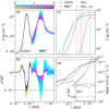 |
Fig. D.1 Effect of different viscosity parameters on the location and evolution of pressure bumps. Panels (a) and (b): Comparison between the models alDZ4 and MREF* (separated by the dotted grey line) in terms of the evolution of the surface density and κ2/Ω2 for a density bump placed by the respective outburst cycles. The depicted time frame is the same for both models and begins at a time t0 at which both models have roughly the same minimum value of κ2/Ω2. The time t1 = t0 + ∆t has been chosen arbitrarily. Panels (c) and (d): Surface density and the radial gradient of the vortensity for four different models in the radial range of the DZIE. The vertical dashed lines in panel (c) mark the positions of the inner pressure bumps in the respective models of the same colour. The inset panel (d1 ) presents κ2/Ω2 for the model alDZ4 around the position of the vortensity minimum. The dashed green lines in panels (b) and (d1) indicate the upper limit for the halfway-to-Rayleigh criterion. |
To investigate the effect of different parameters describing the behaviour of α, we constructed two additional models. alDZ4 has the same configuration as MREF* but with a lower value of αDZ of 10−4, and FULL_25 is equivalent to the FULL model, but with a sharper transition at the DZIE with TΔ = 25 K in Eq. (11). Both models show the same phenomenology concerning the MRI-triggered outburst as the other simulations analysed in this work and Paper I. Panels (a) and (b) of Fig. D.1 compare the evolution of a density bump placed in the respective inner discs of the models alDZ4 and MREF* by burst cycles. The time frame shown from t0 to t1 corresponds to around 95 orbits at 0.5 AU. At this location, the time frame is equivalent to 6 · 10−4tν and 4.8 ∙ 10−5tν for MREF* and alDZ4, respectively, with tν = r2/ν being the viscous timescale. While the density bump disperses significantly during this time in MREF*, there is no visible change in alDZ4. However, panel (b) shows that even for the slowly evolving alDZ4, the bump becomes stable to RWI after approximately 1/3 of the displayed time frame.
Panel (c) compares the surface density structure and the locations of the midplane pressure maxima at the DZIE during the quiescent phases for the four models. As expected, the FULL model exhibits a smaller gradient and a more smoothed-out transition between the MRI active and dead zone. Consequently, the inner pressure bump is placed at almost the same location as in the MREF* model, although the inner dust rim is much closer to the star in FULL. Only if the transition range is reset to the same width as in MREF*, the pressure bump emerges at smaller radii, as modelled in FULL_25. A possible consequence of this shift in the location of the pressure bump could be that the MRI can be activated (and the burst cycle initiated) even sooner than in the FULL model due to the critical surface density being lower.
In alDZ4, the DZIE and the corresponding pressure maximum move further outwards in the quiescent phase than in models with a higher αDZ. Since MREF* and alDZ4 have the same opacity description and equal values of αMRI,  is also very similar since its value depends on the balance between the viscous heating of the MRI active disc and the radiative cooling. Consequently, the surface density profiles at the beginning of the quiescent phase are also approximately the same in both models. However, since the ratio αMRI/αDZ is larger by an order of magnitude in alDZ4, the density in the irradiated MRI active region during quiescence is much lower, decreasing its optical thickness, allowing the stellar radiation to penetrate deeper into the disc and to push the DZIE further outwards.
Another consequence of the larger αMRI/αDZ ratio is a higher efficiency of the mass accumulation in the inner dead zone due to the exacerbated difference in angular momentum transport between the MRI active and inactive zones. This results in a stronger pressure and density bump, which could bring the DZIE closer to RWI. Panel (d) of Fig. D.1 shows the radial gradient of the vortensity of the four different models. The alDZ4 model does indeed exhibit a vortensity minimum at the DZIE, fulfilling the Lovelace criterion. However, the inset panel (d1) indicates that this structure is still far away from meeting the halfway-to-Rayleigh condition and possibly remains stable. However, lower values of αDZ require higher surface densities to trigger a burst cycle, which could possibly also facilitate the onset of RWI. In the snapshot of alDZ4 shown in Fig. D.1, the model has not reached t = tTI after the quiescent phase due to computation time restrictions. Therefore, the susceptibility of the DZIE to RWI in this model is possibly underestimated. A proper assessment of these results requires simulations in non-axisymmetry.
Appendix E Delayed MRI saturation
To analyse the interplay between the non-instantaneous saturation of the MRI and the outburst mechanism, we adopted an approach similar to the method used by Zhu et al. (2010). We constructed additional simulations in which the prescription of the stress-to-pressure ratio was complemented with a delay factor ξ,
 (E.1)
(E.1)
where ξ follows the evolution equation,
![Mathematical equation: \frac{\partial \xi}{\partial t}= \begin{cases} \frac{1}{\alpha_\mathrm{MRI}-\alpha_\mathrm{DZ}} \, \left [ \mathrm{exp} \left ( 6.253 \, \frac{\Omega}{2\pi m} \alpha_\mathrm{del} \right ) -1 \right ] \vspace{0.1cm}\\ \hspace{2.5cm} \cdot \frac{1}{2} \left [ 1+ \mathrm{tanh} \left ( \frac{0.8 \alpha_1-\alpha_\mathrm{del}}{0.25 \alpha_1} \right ) \right ] &\text{for $\xi < \xi_1$} \\ & \\ -\frac{1}{\alpha_\mathrm{MRI}-\alpha_\mathrm{DZ}} \vspace{0.1cm} \\ \hspace{0.3cm} \cdot \left ( \mathrm{exp} \left [ 4.57 \, \frac{\Omega}{2\pi m} (\alpha_\mathrm{MRI}+\alpha_\mathrm{DZ} -\alpha_\mathrm{del}) \right ]-1 \right ) &\text{for $\xi > \xi_1$} \\ & \\ 0 & \text{for $\xi = \xi_1$} \end{cases}\; ,](/articles/aa/full_html/2026/03/aa57408-25/aa57408-25-eq59.png) (E.2)
(E.2)
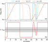 |
Fig. E.1 Demonstration of the effect of delayed MRI-saturation. Panel (a): Temporal evolution of α between its minimum (dead zone) value αDZ and its maximum (fully MRI active) value αMRI in response to an artificial temperature evolution shown in panel (b). The dashed black line in panel (b) marks the MRI activation temperature TMRI, while the grey shaded area indicates the smoothing range around TMRI, determined by TΔ. |
with
![Mathematical equation: \xi_1 = \frac{1}{2} \left [1 - \mathrm{tanh}\left ( \frac{T_\mathrm{MRI}-T_\mathrm{g}}{T_\Delta}\right)\right] ,](/articles/aa/full_html/2026/03/aa57408-25/aa57408-25-eq60.png) (E.3)
(E.3)
and
 (E.4)
(E.4)
In this context, ξ acts as a weight function that changes its value towards ξ1, which is the standard smoothing factor included in Eq. (11). ξ ensures that the time it takes for α to transition between αMRI and αDZ after a rapid change in temperature is equal to m orbits. As initial values, we set ξ = ξ1.
Figure E.1 visualises the behaviour of α in time according to Eq. (E.1) for saturation timescales of zero, three and ten orbits. After a quick increase of the temperature above TMRI, α increases exponentially with varying slopes, dependent on the chosen timescale. The increase tapers off shortly before saturation is reached. This behaviour mimics the growth of the MRI, as investigated in e.g. Hawley & Balbus (1991) and Flock et al. (2010). Rapid oscillations in temperature may remain mostly unrecognised by the viscosity in models with long MRI saturation timescales.
We investigated the consequences of the gradual saturation of the MRI by setting up two additional models, FULL_DEL(3) and FULL_DEL(10), which incorporated the description of α via Eq. (E.1) with saturation times of three and ten local orbits, respectively. Since the MRI transition stays approximately static during quiescence, the following analysis focuses on the burst phase.
Figure E.2 shows the temporal evolution of the bursts occurring in models with various MRI saturation timescales. Panel (a) indicates that the FULL_DEL models still involve a reflare behaviour. However, the individual flares last longer with increasing saturation time due to the advancements of both the heating and the cooling fronts being slowed down. Since the high-state of the burst phase is governed by the same αMRI in all cases, a larger total amount of mass is accreted onto the star per flare in the FULL_DEL models. Hence, fewer reflares occur as the saturation time increases.
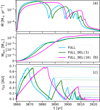 |
Fig. E.2 Effect of different MRI saturation times during a burst cycle. Panels (a), (b), and (c): Accretion rate, the total accreted mass, and the position of the midplane DZIE, respectively, for models with instantaneous saturation (FULL) and saturation over the course of three (FULL_DEL(3)) and ten (FULL_DEL(10)) local orbits. The small dots in panel (c) mark the positions of midplane pressure maxima. |
The same is also discernible in panel (b), where the cumulative total mass accreted on the star is displayed. While the differences between FULL and FULL_DEL(3) are small, the significant delay in MRI saturation in FULL_DEL(10) leads to more total mass having been accreted at the end of the burst cycle.
The MRI activation front at the midplane of the first flare of the accretion event reaches approximately the same distance in all three models, as illustrated in panel (c). Consequently, the outermost pressure bumps are located at the same radii as well. Due to the decreased number of reflares, the models with larger MRI saturation times produce fewer pressure maxima in the dead zone, with only two being created during the burst in the FULL_DEL(10) model.
Appendix F Under-relaxation scheme
The non-linearities introduced in the radiative transport equations by the temperature- and pressure-dependence of the opacities can lead to large oscillations in the solutions found for the total energy and, ultimately, the temperature. Since resolving these non-linear effects by significantly reducing the timestep while still allowing long-term simulations is unfeasible, it was necessary to suppress these oscillations in time. Furthermore, our numerical scheme included a linearisation of the terms proportional to  appearing in Eqs. 1 and 2 (adopted from Commerçon et al. 2011), which is only valid if the relative change in temperature between two subsequent timesteps is small (for details, we refer to Flock et al. 2013, Appendix A). For these purposes, we implemented an under-relaxation scheme for the temperature and both mean opacities in the following way,
 (F.1)
(F.1)
 (F.2)
(F.2)
where δt is the timestep and  and
and  are the solutions for the temperature and opacities for the next timestep as found by the numerical solver. ιT,κ can be regarded as a percentage of the offset between the current values and the newly evaluated solution. With this description, the solver algorithm was forced to adopt values that do not deviate from the current solutions to an extreme extent, while still allowing the quantities to evolve towards any value without numerical restriction. We chose the constant factor ι0 to be between 1/5 and 2/5 for all models.
The oscillations only occur in the optically thin, dust-free regions of the disc. Therefore, the under-relaxation scheme is only applied in numerical cells where fD2G ≈ 0 and ρ < 7.5 ∙ 10−11g cm−3. The effect of this method is illustrated in Fig. F.1. Panel (a) shows the manifestation of the strong oscillations in temperature in the optically thin regions by comparing two models with and without the effect of the under-relaxation scheme, respectively. The radial temperature profiles of these two models at a height of z/r = 0.125 are depicted in panel (b) as the red and orange lines, respectively. The blue profile shows an intermediate state with a less restrictive under-relaxation description, where small oscillations still occur in specific regions (displayed in the inset panel b1). The analytical equilibrium temperature solution shown in green was calculated with Eq. (G.3), considering all of the included terms (contribution of dust, pressure-dependence of the opacities and optical depth effects). The numerical temperature profile resulting from the under-relaxed model with ι0 = 1/5 is in excellent agreement with the analytical solution.
Appendix G Equilibrium temperature with binned frequency-dependent irradiation
In order to find an analytic expression for the equilibrium temperature in the optically thin, irradiated medium in the most general case, we equate the heating rate Q+ = ρκirrFirr to the cooling rate Q− = ρκpFem, with κP being the total effective Planck mean opacity (Sect. 2.2), κirr the irradiation opacity and Fem the emission flux. Considering the binned frequency dependence of the irradiation, the product κirrFirr has to be evaluated in every bin separately before summing over all bins. Using the spectral weights of the frequency bins introduced in Eq. (B.6) and considering the attenuation of the irradiation up to the evaluation radius r, the heating rate is expressed as
 (G.1)
(G.1)
where κ(νi, Tg, Pg) = Kg(νi, Tg, Pg) + fD2GκD(νi) takes the contribution of both gas and dust into account. With F0 = (R*/r)2 σSBT*4, we define the irradiation opacity κirr(Tg, Pg) as
 (G.2)
(G.2)
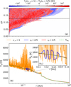 |
Fig. F.1 Visualisation of the effect of the under-relaxation scheme. Panel (a): Map of the temperature residuals between states calculated with (ι0 = 1/5) and without (ιT,κ = 1) under-relaxation for the upper hemisphere of the FULL model in quiescence. Radial temperature profiles for these two states have been extracted at a height of z/r = 0.125 (dashed black line) and are shown in panel (b). The blue curve represents an additional state resulting from a larger under-relaxation parameter ι0 = 2/5. The profile of the equilibrium temperature evaluated at every radius with Eq. (G.3) is shown as the dashed green line. Panel (b1): Magnification of the region where the more generous underrelaxation description still deviates from the equilibrium solution. |
In the case of grey irradiation, the irradiation opacity can be simplified to κirr(Tg, Pg) = κP(T*, Pg). Identifying the volumetric emission rate of the medium, assuming black-body behaviour and no re-absorption of emitted radiation, with  , setting Q+ = Q− and solving for Tg = Teq, we arrive at the final expression for the equilibrium temperature (analogous to Chiang & Goldreich 1997),
 (G.3)
(G.3)
Appendix H Comments on timescales
As described in Sect. 4.4, the inclusion of mean and frequencydependent dust and gas opacities significantly increases the computational cost of the models. While it was possible to include the entire quiescent phase in addition to the two burst phases in the MREF* model, the simulation of the long quiescent phase had to be artificially accelerated in FULL. For that purpose, we let the model relax into the quiescent state after the initial burst cycle before we accelerated the computation by switching to a simple Euler solver (in contrast to the second-order Runge-Kutta method normally used for all models) and shortening the viscous evolution timescale by increasing both5 αMRI and αDZ by a factor of 1.3. Since the disc structure is not subject to any rapid changes during quiescence, the simpler solver algorithm still captured the relevant processes to sufficient accuracy.
We used the slope of the accretion rate evolution depicted in panel (b) of Fig. 6 as a diagnostic for when the relaxation after the initial burst cycle has been completed. Taking the MREF* model as a template, we switched on the acceleration as soon as the slope of the accretion rate evolution became constant in time. The acceleration was stopped when the model entered the next burst phase. At this point, we reverted to our standard computational method, restored the α parameters to their normal values, and let the model relax again until the accretion rate evolution resumed the same slope as before the acceleration. The next burst cycle then emerged soon after this relaxation phase was completed at a critical accretion rate. The dashed line in panel (b) of Fig. 6 shows the interpolated accretion rate, having the slope of the relaxed quiescent model, during the time frame of the acceleration.
This method of shortening the computational time might alter the actual timescale of the quiescent phase between burst cycles. However, as elaborated on in Sect. 4.5, the duration of the quiescent phase may also be subject to other processes or interactions that are not considered in our models but could disturb the equilibrium state in the inner dead zone and ignite bursts at different stages. Therefore, predicting the quiescent timescale is a complex endeavour, especially in non-isolated systems.
Appendix I Relevant expressions for RWI conditions
The vortensity q is given as the fraction between the vorticity and the surface density,
 (I.1)
(I.1)
with the squared epicyclic frequency being defined as
 (I.2)
(I.2)
The Gaussian profile fitted to the density bumps in our models is given as (analogous to Ono et al. 2016)
![Mathematical equation: \Sigma=\Sigma_\mathrm{bg}\left [1+A\;\mathrm{exp}\left(-\frac{(r-r_\mathrm{bump})^2}{2W^2} \right) \right] \; ,](/articles/aa/full_html/2026/03/aa57408-25/aa57408-25-eq73.png) (I.3)
(I.3)
with Σbg = ∑0rb being the background surface density profile (without bumps), where Σ0 and b are the background surface density at the bump location rbump and the slope of the background profile, respectively.
All Tables
All Figures
|
Fig. 1 Planck (panels a and b) and Rosseland (panels c and d) mean opacities. Panels a and c: maps of the temperature- and pressure-dependent gas mean opacities. The pink lines represent the dust mean opacities as functions of temperature. Panels b and d: final effective mean opacities, with the lime-coloured contour indicating the dust sublimation temperature, TS, for each pressure value. The white and black dots mark the temperaturepressure pairs that occur in our simulations, representing a snapshot of the quiescent and the outburst stage, respectively. |
| In the text | |
|
Fig. 2 Frequency-dependent gas and dust opacities in relation to the irradiating blackbody spectrum of the central star. The black lines indicate the Planck function of the irradiation, where the dash-dotted line represents the star during the quiescent phase (with negligible contribution from the accretion luminosity), whereas the dashed line shows the irradiating spectrum that includes the effect of the maximum accretion luminosity occurring in our models. The separation of the frequency space into the 50 bins is indicated by the thin vertical lines, where each bin is coloured according to its relative spectral weight. The orange crosses mark the dust opacities in their respective bins, multiplied by the maximum dust-to-gas mass ratio f0. The gas opacities in each bin were evaluated for a density of 10−10 g cm−3 and are shown for two representative temperatures: 1000 K (blue crosses) and 3000 K (magenta crosses). |
| In the text | |
|
Fig. 3 Comparison between the models MREF* and DUST. Panel a: map of the temperature difference between the two models at a stage when the MRI active region has reached its largest extent during a burst. The black, green, and magenta contour lines represent the MRI transition, the dust sublimation front, and the τrad = 1 surface, respectively, where the dashed lines correspond to DUST and the solid lines to MREF*. Panels b and c: surface density and total vertical optical depth, respectively, of both models at two different stages: the initial hydrostatic structure (blue), and the state after the initial burst, when most of the density bumps have diffused (red). |
| In the text | |
|
Fig. 4 Differences between the models DUST and FULL during quiescence (panel a) and outburst (panel b). The coloured contour lines represent the same transitions as in Fig. 3, with the solid lines corresponding to DUST and the dashed lines to FULL. The upper halves of the panels show the differences in temperature between the two models, while the lower halves depict the absolute temperature of DUST. |
| In the text | |
|
Fig. 5 Evolution of the outburst in the FULL model compared to MREF*. The different columns correspond to different evolutionary stages, starting from the ignition of the burst at t = tTI, chronologically proceeding through the burst stage and ending with the beginning of the next quiescent state at t = tquies. The top row shows the temperature maps of FULL with the black and green contour lines marking the MRI-transition and the dust sublimation front. The middle row depicts the surface densities for both MREF* and FULL at the same stages during their respective evolution. The vertical dotted lines in the first panel indicate the locations of the DZIE in the corresponding model of the same colour. The panels in the second, third, and fourth column also show the respective profiles of |
| In the text | |
|
Fig. 6 Evolution of the surface densities and accretion rates. Panels a and c: space-time diagrams of MREF* and FULL, respectively. The displayed time spans have the same length. The white contours mark the positions of local pressure maxima, while the cyan line indicates the DZIE at the midplane. Panel b: accretion rates for both models over their entire simulation times. The dashed section of the blue line represents the interpolation between the two bursts. Panel d: magnification of the burst occurring in FULL. The vertical dashed lines mark the time of the ignition of the outburst (tTI), the first and second reflections of the heating front (tc1, tc2), the launching of the first reflare (trefl) and the beginning of the quiescent phase (tquies) for FULL. For comparison, the accretion rate resulting from the burst in MREF* is overplotted, shifted in time so that the respective tTI for both models align. |
| In the text | |
|
Fig. 7 Temperature jump as a consequence of the equilibrium temperature degeneracy. Panels a and c: temperature maps of the quiescent phase for the models FULL and NOFREQIRR, respectively. The dashed red lines show the radial profiles of the temperatures at a height of z/r = 0.2 (indicated by the dotted white line). The solution of Eq. (G.3) for Teq at every radius is represented by the blue line. The green contours mark the dust sublimation fronts. Panels b and d: function given in Eq. (13), evaluated at four different radii for both models, respectively. The star-shaped markers indicate which of the available solutions is adopted by the solver at each radius. The same markers were used to locate the respective evaluation radii in panels a and c. |
| In the text | |
|
Fig. 8 Different τ = 1 lines for a disc in quiescence (panels a and c) and in outburst (panels b and d) shown atop the underlying temperature structure for the model FULL. In panels a and b, the dashed blue lines mark the τvert(ν) = 1 surfaces for different wavelengths, which are indicated in the labels in units of μm. The dashed lines in panels c and d show the locations of the τrad(ν) = 1 transitions for the stellar irradiation for several representative wavelength bins with the respective central wavelengths in μm marked in the labels. The colour of the dashed lines indicates the relative spectral weight of the bin. Additionally, each panel includes the dust sublimation front as the green line and the τrad,tot = 1 line for the total radial optical depth in red. |
| In the text | |
|
Fig. 9 Analysis of the stability criteria for the density maxima generated during the outburst in the FULL model. Top three panels: temporal evolution of the surface density Σ (panel a), the parameter κ2/Ω2 (panel b), and the vortensity q (panel c). These are shown as snapshots during the time frame starting from the ignition of the burst (t = tTI, blue line) until the first density bump has reached its outermost position and κ2/Ω2 becomes positive (brown line). Additionally, the pink line represents the disc at t = tquies. The dashed green line in panels b and (b1) indicates the halfway-to-Rayleigh stability threshold. Bottom three panels: Same three quantities, but zoomed into the radial region where the first density bump is located. The colour-coded time frame begins at the moment when min(κ2/Ω2) > 0 and includes the transition from instability to stability according to the halfway-to-Rayleigh criterion, reached at t = 3877.7 yr (orange line in panels a1, b1, and c1 and in the colour bar). Quantities in panel b, (b1), panel c, and (c1) are depicted on a logarithmic scale with a linear transition around zero, indicated by the grey shaded region. |
| In the text | |
|
Fig. 10 Differences in the SEDs between the MREF* and FULL models during the quiescent and outburst phases. The shaded areas mark the wavelength regions covered by the various infrared bands. |
| In the text | |
|
Fig. 11 S-curve behaviour with respect to the MRI-activated TI and evolution of the inner disc during quiescence. Panel a: S-curves of MREF*, DUST, and FULL, extracted from the respective quiescent phases (for MREF* and FULL) compared with the main flares of the accretion events (for all three models) at a radius of 0.2 AU. The arrows along the curves indicate the direction of evolution. The dashed black lines mark the critical values of the surface densities at which the respective upper branches end. The panel also includes the upper branches of the S-curves for the DUST and FULL models at r = 0.08 AU. Panel b: evolution of the surface density during the quiescent phase of FULL. The dashed yellow line is the approximate profile of the hydrostatic structure the disc would adopt if no TI were to occur. |
| In the text | |
|
Fig. D.1 Effect of different viscosity parameters on the location and evolution of pressure bumps. Panels (a) and (b): Comparison between the models alDZ4 and MREF* (separated by the dotted grey line) in terms of the evolution of the surface density and κ2/Ω2 for a density bump placed by the respective outburst cycles. The depicted time frame is the same for both models and begins at a time t0 at which both models have roughly the same minimum value of κ2/Ω2. The time t1 = t0 + ∆t has been chosen arbitrarily. Panels (c) and (d): Surface density and the radial gradient of the vortensity for four different models in the radial range of the DZIE. The vertical dashed lines in panel (c) mark the positions of the inner pressure bumps in the respective models of the same colour. The inset panel (d1 ) presents κ2/Ω2 for the model alDZ4 around the position of the vortensity minimum. The dashed green lines in panels (b) and (d1) indicate the upper limit for the halfway-to-Rayleigh criterion. |
| In the text | |
|
Fig. E.1 Demonstration of the effect of delayed MRI-saturation. Panel (a): Temporal evolution of α between its minimum (dead zone) value αDZ and its maximum (fully MRI active) value αMRI in response to an artificial temperature evolution shown in panel (b). The dashed black line in panel (b) marks the MRI activation temperature TMRI, while the grey shaded area indicates the smoothing range around TMRI, determined by TΔ. |
| In the text | |
|
Fig. E.2 Effect of different MRI saturation times during a burst cycle. Panels (a), (b), and (c): Accretion rate, the total accreted mass, and the position of the midplane DZIE, respectively, for models with instantaneous saturation (FULL) and saturation over the course of three (FULL_DEL(3)) and ten (FULL_DEL(10)) local orbits. The small dots in panel (c) mark the positions of midplane pressure maxima. |
| In the text | |
|
Fig. F.1 Visualisation of the effect of the under-relaxation scheme. Panel (a): Map of the temperature residuals between states calculated with (ι0 = 1/5) and without (ιT,κ = 1) under-relaxation for the upper hemisphere of the FULL model in quiescence. Radial temperature profiles for these two states have been extracted at a height of z/r = 0.125 (dashed black line) and are shown in panel (b). The blue curve represents an additional state resulting from a larger under-relaxation parameter ι0 = 2/5. The profile of the equilibrium temperature evaluated at every radius with Eq. (G.3) is shown as the dashed green line. Panel (b1): Magnification of the region where the more generous underrelaxation description still deviates from the equilibrium solution. |
| In the text | |
Current usage metrics show cumulative count of Article Views (full-text article views including HTML views, PDF and ePub downloads, according to the available data) and Abstracts Views on Vision4Press platform.
Data correspond to usage on the plateform after 2015. The current usage metrics is available 48-96 hours after online publication and is updated daily on week days.
Initial download of the metrics may take a while.