| Issue |
A&A
Volume 707, March 2026
|
|
|---|---|---|
| Article Number | A327 | |
| Number of page(s) | 18 | |
| Section | Interstellar and circumstellar matter | |
| DOI | https://doi.org/10.1051/0004-6361/202558285 | |
| Published online | 18 March 2026 | |
The GUAPOS project
VII. Physical structure and molecular environment of the G31.41+0.31 HII region★
1
INAF, Osservatorio Astrofisico di Arcetri,
Largo E. Fermi 5,
50125
Firenze,
Italy
2
Centro de Astrobiología (CAB), CSIC-INTA,
Carretera de Ajalvir km 4, Torrejón de Ardoz,
28850
Madrid,
Spain
3
Institut de Ciències de l’Espai (ICE), CSIC,
Campus UAB, Carrer de Can Magrans s/n,
08193
Bellaterra,
Barcelona,
Spain
4
Institut d’Estudis Espacials de Catalunya (IEEC),
E-08860,
Castelldefels,
Barcelona,
Spain
5
INAF, Istituto di Astrofisica e Planetologia Spaziale,
Via Fosso del Cavaliere 100,
00133
Roma,
Italy
★★ Corresponding author: This email address is being protected from spambots. You need JavaScript enabled to view it.
Received:
27
November
2025
Accepted:
18
February
2026
Abstract
Context. Ionised regions around OB-type stars, formed at an early stage of their evolution, are important in the investigation of the formation processes of these objects. Thus far, however, only a few observations of their physical structure and interaction with the parental molecular cloud have been carried out. The high resolution and high sensitivity of new instruments such as ALMA and the upgraded VLA allow us to fill in this knowledge gap.
Aims. We investigate the well-known core-halo ultracompact HII region G31.41+0.31 and the surrounding molecular clump to determine the density and temperature of both the ionised and neutral gas, and to possibly obtain a 3D picture of their spacial distribution.
Methods. We took advantage of the full-band frequency coverage at 3 mm obtained with ALMA for the GUAPOS project to image the emission of a plethora of hydrogen recombination lines towards the G31.41+0.31 HII region, as well as several molecular transitions that serve as tracers of medium-density (~104−106 cm−3) gas. The line data are complemented by continuum measurements obtained with the VLA at 1 cm and 7 mm. By fitting these lines with a model that takes into account non-local thermal equilibrium (NLTE) effects, we were able to investigate the density and temperature structure and the velocity field of the region.
Results. Our findings, based on a model fit accounting for NLTE effects, indicate that the electron temperature of the HII region mostly spans a range between 5000 and 6000 K, while the density varies between 2500 and 7500 cm−3. All in all, the distribution of these parameters, along with the corresponding velocity field hint at a cometary shaped HII region expanding away from the observer to the NW. The molecular gas appears to be still infalling towards the peak of the UC HII region, while its density and temperature are consistent with pressure confinement of the ionised gas to the SE.
Key words: stars: formation / stars: massive / HII regions / ISM: supernova remnants / ISM: individual objects: G31.41+0.31
Based on observations carried out with ALMA and the VLA.
© The Authors 2026
 Open Access article, published by EDP Sciences, under the terms of the Creative Commons Attribution License (https://creativecommons.org/licenses/by/4.0), which permits unrestricted use, distribution, and reproduction in any medium, provided the original work is properly cited.
This article is published in open access under the Subscribe to Open model. This email address is being protected from spambots. You need JavaScript enabled to view it. to support open access publication.
1 Introduction
Ultracompact (UC) HII regions are early manifestations of newly formed early-type stars, which ionise the surrounding environment with their powerful Lyman continuum flux, shortward of 912 Å. The pivotal Very Large Array (VLA) survey by (Wood & Churchwell 1989a) and their subsequent study on the far-infrared (IR) colours of UC HII regions (Wood & Churchwell 1989b) made it possible to identify a conspicuous number of these sources and propose a classification based on their morphology. Since then, a number of observations have been performed to investigate the structure and evolution of these intriguing objects, but the limited sensitivity, uv coverage, and frequency coverage of the available interferometers (especially at millimetre and submillimetre wavelengths) hindered the simultaneous observation of both the ionised gas and its molecular surroundings. Measuring many different tracers at the same time allows us to obtain very accurate relative positions and intensities, which are instead affected by significant uncertainties when comparing data obtained with different instruments and/or at different times. It is important to investigate not only the structure of the ionised and molecular components, but also their mutual interaction to understand the evolution of UC HII regions in such a complex environment, as suggested by theoretical studies (e.g. Peters et al. 2010a,b,c).
The advent of new-generation instruments such as the upgraded Karl Jansky Very Large Array (VLA) and the Atacama Large Millimeter and submillimeter Array (ALMA) has dramatically improved the situation. It is now possible to cover broad frequency ranges in a reasonable observing time, thereby allowing us to obtain simultaneous measurements via many different molecular tracers and recombination lines (tracing the ionised gas) as well as high-sensitivity continuum images. With this in mind, we decided to carry out an in-depth study of the well known high-mass star-forming region G31.41+0.31, located at a distance of 3.75 kpc (Immer et al. 2019). This star-forming region contains an UC HII region, classified as a ‘core-halo’ by (Wood & Churchwell 1989a), and a bright hot molecular core (HMC). The latter has been the subject of a series of articles aimed
at investigating its physical structure and chemical composition (Cesaroni et al. 1994a,b, 1998, 2010, 2011, 2017; Beltrán et al. 2004, 2005; Beltrán et al. 2009, 2018, 2019, 2021, 2022a,b, 2024; Rivilla et al. 2017). The goal of our ALMA project G31.41+0.31 Unbiased ALMA sPectral Observational Survey (GUAPOS) is to cover the whole bandwidth of the 3 mm receivers of the interferometer, which allow for the detection of a plethora of transitions from a variety of molecular species (Mininni et al. 2020, 2023; Colzi et al. 2021; Fontani et al. 2024; López-Gallifa et al. 2024, 2025). While it was mainly intended to be a line survey for studying the rich chemistry of HMCs, the detection of many hydrogen recombination lines and several rotational transitions tracing the extended molecular gas also allows us to shed light on the internal physical structure of the HII region and its parental molecular clump.
In this article, we present the observations performed with ALMA and the VLA (Sect. 2). We describe the results obtained (Sect. 3), derive a number of physical parameters of the ionised and neutral gas (Sect. 4), and examine the complex structure of the region with a special focus on the interaction between the HII region and its molecular surroundings (Sect. 5).
2 Observations and data reduction
In the following, we describe the observations performed towards G31.41+0.31 with the ALMA and VLA interferometers, including data from the VLA archive as well.
2.1 Atacama Large Millimeter and submillimeter Array
The data used in this study are part of the GUAPOS project (2017.1.00501.S, PI: M. T. Beltrán) and we refer to (Mininni et al. 2020) for the observational details and the data reduction procedures adopted. Here, we only provide the basic information.
The ALMA observations of G31.41+0.31 were performed in band 3 with a phase centre of α(ICRS)=18h47m34s315 and δ(ICRS)=−01°12′45″.9. Source J1751+0939 was used as bandpass and flux calibrator, while the phase calibrator was J1851+0035. Nine correlator configurations, each consisting of four units of 1.875 GHz, were necessary to cover the whole receiver bandwidth between 84.05 and 115.91 GHz, with a spectral resolution of 0.488 MHz, corresponding to −1.3-1.7 km s−1 depending on the frequency. Calibration and data reduction were performed with the Common Astronomy Software Appli-cations1 (CASA; McMullin et al. 2007) and the maps were all cleaned with Briggs robust=0.5 weighting and a circular synthesised beam with full width at half power (FWHP) of 1″.2, corresponding to 4500 au. The continuum maps and corresponding continuum-subtracted channel maps were created with the software STATCONT2 (Sánchez-Monge et al. 2018).
2.2 Karl Jansky Very Large Array
The Ka band observations of G31.41+0.31 (project 16A-181, PI: V. M. Rivilla) were performed on March 3, 8, and 22, 2016 in the C-array configuration. The equatorial coordinates of the phase centre were α(J2000)=18h47m34s.315 and δ(J2000)=−01°12′45″.9. The total observing bandwidth (per polarisation) used to measure the continuum emission was ~1.8 GHz.
The primary flux calibrator and the phase calibrator were 3C286 and J1851+0035, respectively. The CASA software was used for calibration and data reduction and the data were calibrated with the VLA pipeline. The maps were made with task tclean of CASA using Briggs robust=0.5 weighting. For the sake of comparison with the ALMA data, we also selected the uv range 4.9-257 klambda and a circular clean beam with FWHP=1″.2. The resulting root-mean-square (RMS) noise was ~0.1 mJy/beam.
We also made use of archival data at 7 mm (Project 23A-066, PI: H. Liu). In this case, the observations were performed in the B-array configuration on January 14 and May 3, 6, 9, 10, and 12 2023. The phase centre was α(J2000)=18h47m34S308 and δ(J2000)=−01°12′45″.9. The total observing bandwidth (per polarisation) used to measure the continuum emission was −7 GHz. The flux and phase calibrator swere, respectively, 3C286 and J1851+0035. The calibrated data were obtained directly from the NRAO archive and the continuum maps were made with the CASA software using task tclean with Briggs robust=0.5 weighting. The resulting image has a synthesised beam FWHP of 0″.210×0″.169 and PA= −0°.51. The 1σ RMS noise is −0.01 mJy/beam.
3 Results
In the following, we present the outcome of our observations separately for the continuum, recombination lines, and molecular lines.
3.1 Continuum emission
The 1 cm and 7 mm continuum maps shown in Fig. 1a trace the free-free emission from the ionised gas, confirming the core-halo morphology identified by (Wood & Churchwell 1989a). Hereafter, we refer to the ‘core’ as the ‘UC HII region’ to distinguish it from the ‘halo’, namely, the extended ionised component; we use the more generic term ‘HII region’ to indicate the whole core+halo system. In particular, the sub-arcsecond resolution of the 7 mm image reveals the inner structure of the UC HII region, which presents an asymmetry hinting at a cometary shape (see Fig. 1b) with the head pointing approximately eastwards. Another interesting feature seen at 7 mm is the presence of four emission peaks inside the HMC, whose approximate border is outlined by the dotted contour in the figure. The latter corresponds to the 10% contour level of the C33S(2-1) integrated emission (see Sects. 3.3 and 4.2). These sources correspond to those revealed by (Cesaroni et al. 2010) and (Beltrán et al. 2021) and might be associated with newly formed deeply embedded massive stars, as discussed by these authors.
From the ALMA data, we obtained a continuum map by averaging the emission over the frequency range covered by the GUAPOS project after removing the line emission as explained in Sect. 2.1. In the 3 mm map presented in Fig. 1c, we can clearly see a pronounced peak of emission corresponding to the HMC, which proves that the observed flux is mostly contributed by dust thermal emission.
It is interesting to compare our maps with FIR images tracing the emission from the dusty molecular clump enshrouding the HII region. Figure 2 presents an overlay between the 1 cm map and images of the region at 8 μm from the Spitzer/GLIMPSE database (Werner et al. 2004; Fazio et al. 2004; Benjamin et al. 2003) and at 70 μm from the Herschel/Hi-GAL survey (Molinari et al. 2010). The complexity of the region shows up clearly in this figure, where the ionised gas appears to be tightly confined due to the presence of a molecular cloud on the eastern side revealed by the heavily extincted region elongated in the N-S direction and traced also by the N2H+ (1-0) line emission (see Beltrán et al. 2022b). Noticeably, the HMC is undetected at least up to 8 μm, despite its massive and therefore luminous stellar content. This is consistent with the large column densities (≳1024 cm−2) derived in previous studies (see Eq. (3) of Beltrán et al. 2018). The overall picture is suggestive of a champagne flow confined to the east and expanding westwards. We present additional evidence for this interpretation in Sect. 5.2.
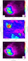 |
Fig. 1 (a) Maps of the 1 cm (colour image and white contours) and 7 mm (black contours) continuum emission imaged with the VLA. The contour levels of the 1 cm map are drawn in the colour scale to the right, while those of the 7 mm map range from 0.08 to 1.88 in steps of 0.3 mJy/beam. The black dotted pattern outlines the approximate border of the HMC (see text). The dashed rectangle frames the region shown in panel b. The synthesised beams (1″.2 at 1 cm and 0″.21×0″.17 with PA −0°.5 at 7 mm) are shown in the bottom-left and -right corners. (b) Enlargement of the region that contains the UC HII region and the HMC, corresponding to the dashed rectangle in panel a. The symbols have the same meaning as in panel a, with the exception of the colour image that shows the 7 mm continuum emission. We note that the colour scale is saturated (the peak emission at 7 mm is 1.96 mJy/beam) to emphasise the structure of the UC HII region. (c) Contour map of the 3 mm continuum emission obtained from the ALMA data overlaid on the same 1 cm continuum image as in panel a. Contour levels range from 0.5 to 180 mJy/beam in ten logarithmic steps. The synthesised beam (1″.2) is the same for both maps and is shown in the bottom-right corner. |
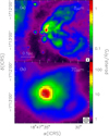 |
Fig. 2 (a) Overlay of the 1 cm map of Fig. 1 (contours) and the 8 μm image from the Spitzer/GLIMPSE database (colour image). Contour levels range from 1 to 28 in steps of 9 mJy/beam. The angular resolution of the latter image is shown in the bottom-right corner. The dotted rectangle outlines the region shown in Figs. 1a and c. (b) Same as panel a, for the 70 μm image obtained from the Herschel/Hi-GAL survey. |
3.2 Recombination lines
Thanks to the broad frequency coverage of the GUAPOS project, we could reveal all of the α, β, and γ recombination lines of hydrogen that fall in the ALMA 3-mm receiver band. The only exceptions were the H38α line, which is heavily blended with the 12CO(1-0) transition, and the H59γ line, which is faint and contaminated by an HCO+ (1-0) absorption feature (see Table 1). No recombination line of elements heavier than hydrogen was detected. In Figs. 3, 4, and 5, we show maps of the integrated intensity, peak velocity, and full width at half maximum (FWHM) of the lines. These parameters were obtained by fitting the spectrum at each pixel of the map with a Gaussian. In this procedure, we rejected the data if less than five channels were above 3σ or the RMS of the residual spectrum (after subtracting the fit) was above three times the noise of the original spectrum. The latter criterion explains why the area corresponding to the HMC is blanked in the maps, as the corresponding spectra present a line forest that introduces a large RMS in the residual spectra.
It is evident that only the α lines trace the whole ionised halo, whereas the γ lines are detected mostly towards the UC HII region. This difference is not surprising as the latter lines are intrinsically fainter than the former. We note that the H54γ line emission is contaminated by the NS J=5/2-3/2 Ω=1/2, F=5/2-3/2 l=f and F=3/2-1/2 l=f hyperfine components. The velocity maps outline a clear gradient with velocity increasing from SSE to NNW. The UC HII region is somehow part of the general trend as we see a velocity gradient across it in the E-W direction, approximately the same as the symmetry axis of the cometary shaped free-free emission (see Sect. 3.1). If we refer the recombination line velocities to the systemic LSR velocity of the HMC (96.5 km s−1; see e.g. Cesaroni et al. 2011), we see that most of the ionised gas is red shifted, which implies that the HII region is expanding away from the dense molecular gas. Such a scenario is consistent with the broad line width observed at the eastern side of the UC HII region (see Fig. 5), which hints at a larger velocity dispersion at the interface between the ionised gas and the dense molecular gas.
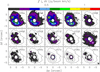 |
Fig. 3 Maps of the integrated emission over the hydrogen recombination lines indicated in the top right corner of each panel. The emission from the HMC is not plotted because the recombination lines are heavily blended with stronger molecular transitions. The circle in the bottomright corner is the synthesised beam. The offsets are relative to the phase centre of the ALMA observations. The emission of the H54γ line is contaminated by two hyperfine components of the NS J = 5/2 → 3/2 transition. |
Hydrogen recombination lines observed in the present study.
3.3 Molecular lines
While the GUAPOS project is mostly focused on HMC tracers, the broad bandwidth covers also other species that allow us to study the more extended molecular clump enshrouding the HII region. For this reason, we looked for rotational transitions of typical medium-density (~104−106 cm−3) tracers. In particular, we selected the lines in Table 2, which were sufficiently intense and not affected by blending with other lines. Figure 6 gives an idea of the distribution of the medium-density molecular gas (traced by H13CO+) with respect to the HII region and shows the four template positions whose spectra are presented in Figs. 7–10. These positions have been chosen at the main peaks of the free-free and H13CO+(1-0) line emission, excluding the HMC due to the complexity of the spectrum. We note that the ‘SW’ position lies very close to the ‘shock region’ studied by (López-Gallifa et al. 2025), also called ‘region 2’ by (Fontani et al. 2024). The line profiles present multiple velocity components in both emission and absorption. It is worth noting that the absorption is seen only towards the bright continuum background of the HII region, which proves that it is real and not a fake feature due to the presence of extended structures resolved out by the interferometer.
Although the complexity of the spectra makes the data interpretation more difficult, the absorption features provide us with useful positional and kinematical information on the neutral gas with respect to the ionised gas. Looking at the spectra towards the UCHII and HII positions (Figs. 7 and 8), we see that in both positions absorption is detected in several lines at about the velocity of the HMC, which suggests that the HMC itself may be part of a molecular clump located between the HII region and the observer. Another interesting feature is the inverse P-Cygni profile seen towards the UC HII region, which might be due to residual infall. Towards the HII region centre (Fig. 8) a broad red-shifted wing is present, which is related to the red lobe of the most prominent bipolar outflow imaged by (Beltrán et al. 2018). The absorption dip, slightly red-shifted with respect to the HMC velocity, is likely due to the bright background continuum emission of the nearby HMC. It is also worth noting that the blue-shifted emission at ~94 km s−1 seen at the S position (Fig. 10) could be due to the molecular cloud imaged by Beltrán et al. (2022b) to the south of the HMC. In Sects. 5.2 and 5.3, we analyse the structure and kinematics of the region in more detail.
Parameters of molecular lines used to study the extended molecular cloud enshrouding the HII region.
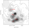 |
Fig. 6 Contour map of the 1 cm continuum emission overlaid on a map of the peak emission in the H13CO+(1-0) line (grey scale). Contour levels range from 1 to 28 in steps of 3 mJy/beam. The crosses and corresponding labels denote the four template positions that the spectra of Figs. 7–10 have been taken towards. |
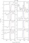 |
Fig. 7 Spectra of various molecular lines (as indicated in each panel) observed towards the UCHII position in Fig. 6 with ICRS coordinates 18h47m34s.555-01° 12′43″.20. The blue dotted and red dashed lines mark, respectively, the systemic LSR velocity of the HMC (96.5 km s−1; Cesaroni et al. 2011) and the peak velocity of the H39α recombination line measured at the given position. |
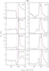 |
Fig. 8 Same as Fig. 7 but for the HII position in Fig. 6 with ICRS coordinates 18h47m34s.415-01°12′46″.95. |
4 Analysis
In this section, we analyze the continuum and line data with the aim to establish the physical properties of both the ionised and molecular components. We also investigate the relationship between them.
4.1 The HII region
From the integrated 1 cm continuum flux over the whole HII region in Fig. 1, we can compute the Lyman continuum photon rate, NLy, needed to ionise the gas. In this calculation we assume that the 1 cm free-free emission is optically thin and the mean electron temperature is 6000 K (see Sect. 4.1.2). We measured a flux density of ~760 mJy within the 3σ contour level of the HII region, corresponding to NLy ≃ 1.5 × 1048 s−1. If the ionisation is attributed to a single star, this value implies a spectral type O8.5 (Panagia 1973) and a stellar luminosity of ~5 × 10⁴ L⊙. (Cesaroni et al. 1994a) calculated a bolometric luminosity from the IRAS fluxes of 6 × 10⁴ L⊙ (after scaling the value to the most recent estimate of 3.75 kpc), only slightly greater (by ~104 L⊙, i.e. ~20%) than that obtained from the Lyman continuum flux.
This result has the two-fold implication that the ionising flux must be mostly due to a single massive star, and the number of Lyman continuum photons absorbed by dust inside the HII region is negligible. This is because, on the one hand, for the same total bolometric luminosity multiple early-type stars would emit less ionising photons with respect to a single star (see e.g. Fig. 7 of Cesaroni et al. 2015); on the other hand (as noted by Wood & Churchwell 1989a), if a significant number of Lyman continuum photons were absorbed by dust inside the HII region, the observed free-free emission should be fainter and suggest a value of the stellar luminosity significantly less than Lbol (see Spitzer 1998).
The previous conclusion, namely, that only one massive star contributes to the bolometric luminosity and Lyman continuum, is challenged by the findings of Cesaroni et al. (2010) and Beltrán et al. (2021). They identified four massive young stellar objects (YSOs) inside the HMC. Being deeply embedded, these (proto)stars cannot be responsible for the ionisation of the HII region, but should contribute to the total luminosity at a level that is much higher than ~104 L⊙ (see above). The solution of this conundrum might be simply related to the uncertainties in the determination of the luminosities and/or to the identification of the embedded YSOs. However, other explanations are also possible. One is provided by the fact that ~1/3 of the compact HII regions appear to be ionised by stars with Lyman continuum luminosities more intense than expected for their spectral types - the so-called ‘Lyman excess’ (Sánchez-Monge et al. 2013; Urquhart et al. 2013; Cesaroni et al. 2015, 2016). If the star ionising the HII region belongs to this type of objects, its contribution to the bolometric luminosity is less than the 5 × 10⁴ L⊙ previously estimated. The other possibility is that part of the stellar photons longward of 912 Å are not absorbed by the dust and are leaking from the clump enshrouding the HII region. This would cause an underestimation of the bolometric luminosity because the latter was computed from the IR emission of the clump. Indeed, the cometary structure of the region is consistent with lower density and, thus, lower opacity, to the NW. A similar situation has been recently proposed for Sgr B2 (see Budaiev et al. 2026), where part of the radiation appears to be escaping even from the densest regions.
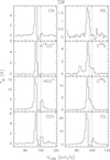 |
Fig. 9 Same as Fig. 7 but for the SW position in Fig. 6 with ICRS coordinates 18h47m34s.245-01°12′50′.25. |
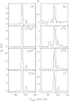 |
Fig. 10 Same as Fig. 7, but for the S position in Fig. 6 with ICRS coordinates 18h47m34s.415-01°12′51″.30. |
4.1.1 The model fit
The detection of many recombination lines provides us with the opportunity to produce temperature and density maps of the HII region. An approximate estimate of the electron temperature can be computed from the line-to-continuum ratio using Eq. (2.124) of (Gordon & Sorochenko 2002), which assumes local thermal equilibrium (LTE). By applying this expression to each line in each pixel of the map, we obtain the electron temperature maps in Fig. 11. Although the maps with the best signal-to-noise ratio appear roughly consistent with each other, suggesting a value of ~7000-8000 K, other maps look significantly different.
Such a discrepancy could be partly due to the fact that our calculation made use of the continuum map at the same frequency as the line map. The millimetre continuum emission is not pure free-free but is known to be contaminated by thermal dust emission (see Sect. 4.2.2). To avoid this problem, we employed the following procedure. For each pixel, we subtracted a constant baseline (0th order polynomial) from the spectrum, thus removing the continuum emission. Then we added an ‘artificial’ continuum level by extrapolating to the corresponding frequency the VLA 1 cm continuum map in Fig. 1, assuming optically thin free-free emission (i.e. flux ∝ ν−0.1). Since the dust emission is negligible at centimeter wavelengths, the continuum level created in this way should correspond to the pure free-free emission emitted at the frequency of the recombination line.
Another explanation for the differences among the maps in Fig. 11 is that non-LTE (NLTE) effects could play an important role. To take these into account, the line+continuum spectra were fitted with the model described in (Cesaroni et al. 2019). which calculates the intensity of the line+continuum emission for given values of the electron density, ne, and temperature, Te. Besides the standard expression for the free-free opacity (e.g. Eq. (A.1a) of Mezger & Henderson 1967), this model uses Eqs. (3.19) and (3.25) of (Brocklehurst et al. 1972) to calculate the emission and absorption coefficients of the recombination line. The b and β coefficients expressing the departure from LTE are computed with the code of (Gordon & Sorochenko 2002). Additional details can be found in (Cesaroni et al. 2019), who assume an expanding shell HII region with constant electron density ne and temperature Te. In our application, we neglected the expansion and assume zero inner radius. The model requires also knowledge of the source distance (3.75 kpc) and HII region radius. In our case, the HII region is far from an ideal uniform sphere and we are thus forced to adopt an approximation to estimate a reasonable value of the radius. Appendix A describes how we calculate the radius, which ranges between 3″.8 (~0.07 pc) and 7″.6 (~0.14 pc).
It is also necessary to have a reasonable guess of the turbulent velocity, Vt, contributing to the Doppler line width as in Eq. (1) of (Gordon & Churchwell 1970):
 (1)
(1)
where k is the Boltzmann constant and m the mass of the atom. This parameter can be derived if two measurements of the line width are available for the same recombination line of two different atomic species. Unfortunately, only hydrogen lines have been detected in our observations of G31.41+0.31, but we have available single-dish spectra of the 55α, 57α, and 58α recombination lines of both hydrogen and helium, obtained with the Yebes 40-m telescope (V. Rivilla, priv. comm.). From these, we obtained the line FWHM with Gaussian fits and computed the weighted mean of the FWHM, which is 22.1 ±0.1 km s−1 for H and 15.4±1.0 km s−1 for He. Then using Eqs. (2) and (3) of (Gordon & Churchwell 1970) we derived mean values over the whole HII region (unresolved in the single-dish beam of 42″–54″) of Vt=9.1±1.4 km s−1 and Te=7200±900 K, a temperature consistent with the values in Fig. 11. For our convenience we defined the ‘turbulent temperature’ as Tt = mH Vt2/(3k) = 5030 ± 1360 K, with a mH mass of the H atom and k Boltzmann constant. Hence, Eq. (1) for the H atom takes the form,
 (2)
(2)
In conclusion, since Te≃Tt within the errors, in our model we assumed Tt=Te all over the HII region.
To get rid of the systemic velocity of the ionised gas and enable comparisons with the model, for each spectrum we subtracted the peak velocity, obtained with a Gaussian fit as explained in Sect. 3.2. Then we convolved the model brightness temperature of the line+continuum emission with the synthesised beam of the observations (1″.2) and computed the χ2 at each position of the map with the expression,
 (3)
(3)
where i indicates the recombination line, j the spectral channel, σi the noise of the spectrum, Vj the channel velocity,  the observed brightness temperature of the line+continuum, and
  that obtained from the model after convolution with the 1″.2 beam. In this calculation we considered only the three strongest recombination lines, namely H39α, H40α, and H41α. The best fit was obtained by minimising χ2 after varying the only two free parameters of the model, ne and Te, over suitable ranges. The uncertainty on the best-fit parameters was estimated with the method of (Lampton et al. 1976).
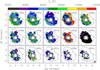 |
Fig. 11 Maps of the electron temperature obtained from the hydrogen recombination lines indicated in the top right corners of the panels, under the LTE approximation. The offsets are relative to the phase centre of the ALMA observations. The contours are the map of the 3 mm continuum emission shown in Fig. 1c, with contour levels ranging from 1.15 to 28.75 in steps of 4.6 mJy/beam. The synthesised beam is shown in the bottomright corner. |
4.1.2 Results of the fit
An example of the χ2 minimisation is illustrated in Fig. 12 for the peak position of the UC HII region, which gives ne= cm−3 and Te=
 K. In the first three panels of Fig. 13 we show the corresponding best-fit spectra (red curves) overlaid on the observed ones. In the other panels of the same figure we also show the model spectra (green curves) for the other recombination lines, computed using the same best-fit parameters. We stress that, although the fit was obtained using only three lines, the match is excellent also for all the others3, which demonstrates the reliability of our method.
The maps of ne and Te in Fig. 14 were obtained by fitting the data only in those pixels where all three fitted lines where clearly detected. The criterion for a detection is that at least five line channels must have intensities above 3σ. We note that all pixels corresponding to the HMC (blanked in Figs. 3–5) were rejected because of heavy overlap with molecular lines, which fill almost the whole observed bandwidth (see Fig. 4 of Mininni et al. 2020). The resulting values are affected by relatively small uncertainties, less than 15% for Te and less than 5% for ne.
The electron temperature is roughly constant all over the HII region, with a mean value of ~6000 K and a median of ~4600 K, comparable to the estimate of 5000 K obtained by (Wood & Churchwell 1991) in a similar object, the cometary UC HII region G29.96-0.02. The prominent peak of ~9000 K close to the SE border of the UC HII region might be real, but it is also possible that it is due to an enhancement of the turbulent velocity at the interface between the UC HII region and the dense molecular gas located to the east. In this case, our assumption of constant Tt=Te could underestimate the contribution of Vt to the line width, thus overestimating the value of Te needed to fit the line profile. The electron density distribution basically mirrors the intensity of the free-free emission, with a main peak toward the UC HII region and a secondary peak between the HMC and the molecular gas located to the south (see Sect. 4.2).
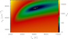 |
Fig. 12 Plot of the χ2 computed from Eq. (3) as a function of electron temperature and density at the peak position of the UC HII region. The white dot marks the minimum and the white contour corresponds to the 1σ confidence level. |
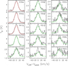 |
Fig. 13 Spectra of the hydrogen recombination lines observed towards the peak of the UC HII region. The name of the line is indicated in the top right corner of each panel. The velocity is relative to the peak velocity of each spectrum, obtained with a Gaussian fit. The red and green curves are the model spectra obtained by fitting only the H39α, H40α, and H41α lines. The H54γ line is contaminated by emission from a molecular line. |
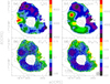 |
Fig. 14 (a) Map of electron temperature of the HII region, obtained by fitting the hydrogen recombination lines with our model (see text). (b) Map of the relative error on the electron temperature. (c) Same as panel a, for the electron number density. (d) Same as panel b, for the electron number density. The angular resolution is represented by the circle in the bottom-right corner. |
4.2 The molecular clump
The continuum and molecular line maps of the GUAPOS project can be used to obtain information on the dusty molecular gas enshrouding the HII region. In the following, we derive estimates of several physical parameters of this neutral component.
4.2.1 Velocity, temperature, and column density from line emission
As discussed in Sect. 3.3, even the molecular lines tracing the extended, lower-density medium have complex spectra with multiple components both in emission and absorption. Since we want to derive maps of physical parameters, it is necessary to select the molecular transitions that are least affected by this problem. After inspecting the most common molecular species, we decided to focus on C33S and CH3CCH, whose emission is dominated by one velocity component, and CN, which shows a prominent absorption feature. The C33S molecule is especially useful to inspect the velocity field of the dense material close to the HII region surface, while CH3CCH is a symmetric top molecule known to be an excellent tool to derive the temperature and column density thanks to its multiple K-ladder components (see e.g. Fontani et al. 2002). The template spectra of the CH3CCH(6-5) transition towards the four positions marked in Fig. 6 are shown in Fig. 15.
We fit Gaussian profiles to the C33S and CH3 CCH spectra pixel by pixel. it is worth noting that overlap with lines of other species may occur only towards the HMC, given the chemical richness of this object (see Fig. 4 of Mininni et al. 2020). For C33S, the hyperfine structure was taken into account in the fitting procedure by fixing the frequency separations and intrinsic relative LTE intensities between the hyperfine components, while assuming the same line width for all of them (see Ungerechts et al. 1986 for a more detailed description of the method). The different K components of CH3CCH where fitted simultaneously by fixing their frequency separations to the laboratory values and assuming the same FWHM for all of them. In Fig. 16, we plot the maps of the parameters derived from the fit to the C33S(2-1) line, namely the opacity of the main hyperfine transition, the peak LSR velocity, and the line width. Figure 17 shows the same quantities for the CH3CCH(6-5) transition, with the only difference that the integral under the K=0 and 1 components is plotted instead of the line opacity.
Both molecules clearly trace the HMC, where the line emission and optical depth attains their maximum, as well as the CH3CCH line width. One can also see that the velocity gradually changes across the HMC, a result consistent with the well known NE-SW velocity gradient observed in several studies (see e.g. Beltrán et al. 2018 and references therein) and interpreted as rotation of the core. We note that this velocity gradient seems to be part of the global velocity field of the region. in fact, on a larger scale the molecular gas appears blue-shifted to the SSW and red-shifted to the NNE, consistent with the findings of (Beltrán et al. 2022b).
The CN(1-0) transition was used to trace the gas seen in absorption against the 3 mm continuum. This is useful to establish the motion of the molecular gas with respect to the ionised gas, as the material seen in absorption is that lying between the HII region and the observer. Given the complex hyperfine structure of the transition, for our purposes we used only the N =1-0, J =1/2-1/2, F=3/2-3/2 component at 113191.2787 MHz, as it is not blended with other lines. In Fig. 18a, we show the map obtained by taking the minimum intensity at each pixel of the map, while the corresponding LSR velocity is shown in Fig. 18b. The two maps are compared to the map of the 3 mm continuum emission and we see that two absorption dips are found toward the UC HII region and the HMC, namely towards the continuum peaks. The most red-shifted absorption is found towards the NE and SW of the HII region, with the region lying between the HMC and the UC HII region being the most blue-shifted.
A comparison of the velocity fields of the molecular and ionised components is presented in Sect. 5.2.
From the integrated intensity maps of the detected CH3CCH(6-5) K components we could obtain column density (NCH3CCH) and rotation temperature (Trot) maps by fitting rotation diagrams pixel by pixel, under the LTE approximation (see e.g. Fontani et al. 2002). The method was applied only to the spectra where at least four (out of six) K lines were detected. The results are shown in Fig. 19 and compared to the map of the 3 mm continuum emission. As expected, both quantities reach their maximum at the position of the HMC, with a temperature of −140 K and a CH3CCH column density of −6 × 1017 cm−2. The mean value of Trot over the HMC is ~90 K, significantly less than that of ~150-165 K estimated by (Beltrán et al. 2018) towards the centre of the HMC (see their Tables 5 and 7). Such a difference is not surprising because these authors observed higher-excitation lines of a less abundant molecule (CH3 CN) with better angular resolution (~0″.2), which makes their observations sensitive to more internal and, hence, hotter parts of the molecular core.
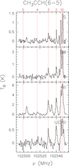 |
Fig. 15 Spectra of the CH3CCH(6-5) transition towards the four positions marked in Fig 6. The K=0-5 components are indicated by the red dotted lines and labelled accordingly. |
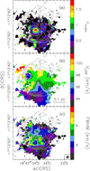 |
Fig. 16 (a) Map of the opacity of the main hyperfine transition of C33S(2-1) (colour image). The contour map represents the 3 mm continuum emission and is the same as in Fig. 1c. (b) Same as panel a, for the LSR velocity. (c) Same as panel a, for the line FWHM. The synthesised beam is shown in the bottom-right corner. |
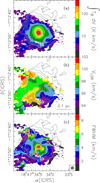 |
Fig. 17 (a) Map of the integrated intensity over the K=0 and 1 components of the CH3CCH(6-5) line (colour image). The contour map represents the 3 mm continuum emission and is the same as in Fig. 1c. (b) Map of the LSR velocity of the CH3CCH(6-5) line obtained by fitting all the K components (see Sect. 4.2.2). (c) Same as panel b, for the line FWHM. The synthesised beam is shown in the bottom-right corner. |
4.2.2 Mass from continuum emission
From our ALMA data we can also obtain an estimate of the mass of the molecular gas enshrouding the HII region. For this purpose we need to subtract the free-free continuum contribution from the 3 mm continuum map of Fig. 1c. We could extrapolate the 1 cm map of Fig. 1 to 3 mm and subtract this from the ALMA map. However, the residual image contains substantial negative structures, most likely due to the different uv coverages of the two maps. We thus preferred to adopt the method proposed by (Cesaroni et al. 2023), who express the ratio between the free-free and dust emissions as a function of the ratio between two observing frequencies and the corresponding spectral index. The assumption is that both the free-free and dust emissions are optically thin, as expected at a wavelength of 3 mm.
In our case, we used the GUAPOS maps at the lowest (84.2 GHz) and highest (115.8 GHz) frequencies. The spectral index was computed from the ratio between the two maps and the correction was obtained by applying Eq. (3) of (Cesaroni et al. 2023) pixel by pixel. This method allows us to separate the contribution of free-free emission to the total flux from that of thermal dust emission, using measurements at two frequencies. Figure 20 shows the spectral index map and the computed maps of pure free-free and thermal dust emission. When applying Eq. (3) of (Cesaroni et al. 2023), we chose a fiducial dust spectral index of 3, corresponding to a dust opacity index of 1. A number of the values on the map in Fig. 20a happen to fall below −0.1 (pure free-free emission) or above +3 (pure dust emission). In these cases the spectral index was reset respectively to −0.1 and +3.
The morphology of the free-free map is qualitatively similar to that of the 1 cm map (Fig. 1), as we can see from the comparison between these two maps shown in Fig. 20b. This gives us confidence with the method used. The dust map peaks at the HMC position, consistent with the continuum images obtained at higher frequencies (see e.g. Beltrán et al. 2021), where the free-free contribution is negligible.
Now, we can estimate the mass of the neutral gas surrounding the HII region from the dust emission map in Fig. 20c and the temperature map obtained from CH3CCH (Fig. 19a). Knowledge of the flux and temperature of the dust allows us to calculate a column density map (see Fig. 21) using, for example, Eq. (2) of Schuller et al. (2009), where we assume temperature equilibrium between dust and gas, a gas-to-dust mass ratio of 100, a mean molecular weight of 2.8, and a dust absorption coefficient κ(ν) = 1 cm2 g−1 (v/230.6 GHz). To calculate the mass of the clump around the HII region we integrated over the whole map in Fig. 21 after removing the contribution of the HMC4, as we are interested only in the large scale structure. The result is ~110 M⊙, which is to be taken as a lower limit to the mass of the whole clump enshrouding the HII region because part of the 3 mm continuum emission is resolved out by ALMA. In fact, (Cesaroni et al. 1991) estimated a clump mass of −290−1100 M⊙ (after re-scaling their values to a distance of 3.75 kpc) from their single-dish observations of C34S.
Finally, from the ratio between the column density maps in Figs. 19c and 21 we could also obtain a map of the CH3CCH abundance with respect to H2 (XCH3CCH). This is shown in Fig. 22. We can infer that XCH3CCH at the position of the HMC is on average 8.2 × 10⁻⁸, slightly higher than the mean value outside the HMC (5.5 × 10⁻⁸).
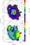 |
Fig. 18 (a) Map (colour image) of the absolute value of the minimum (negative) brightness temperature of the N = 1-0, J =1/2-1/2, F=3/2-3/2 hyperfine component of the CN(1-0) line. (b) Map of the LSR velocity at which the minimum brightness shown in panel a is attained. The synthesised beam is shown in the bottom-right corner. The contour map represents the 3 mm continuum emission and is the same as in Fig. 1c. |
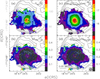 |
Fig. 19 (a) Map (colour image) of the rotational temperature obtained from the rotation diagram of the CH3CCH molecule. Contours represent the same map of the 3 mm continuum emission as in Fig. 1c. (b) Map of the relative error on the rotation temperature. (c) Same as panel a, for the CH3CCH column density. (d) Same as panel b, for the CH3CCH column density. The synthesised beam is shown in the bottom-right corner. |
5 Discussion
In the following, we use our findings to draw conclusions on the 3D structure of the HII region and associated molecular clump.
5.1 Pressure balance
The morphology of the G31.41+0.31 region at radio and IR wavelengths (see Fig. 2) suggests a scenario where the ionised gas is confined to the east by the molecular gas and is expanding approximately to the NW. it is thus interesting to establish whether pressure balance exists at the interface between the ionised gas and the molecular gas. Such a balance is described by the expression,
 (4)
(4)
where ne and Te are the electron number density and temperature, NH2 and Tk the column density and kinetic temperature of the molecular gas, and ∆z the length of the molecular gas along the line of sight. We have ignored the contribution of the magnetic field pressure in this expression. This pressure can be estimated from the expression B2/(8πk), where B is the magnetic field strength and k the Boltzmann constant. According to (Law et al. 2025), the B-field intensity in this region lies in the range 0.04-0.09 mG; hence the maximum magnetic pressure is −2×106 cm−3 K, while the pressure inside the HII region is  K. We conclude that the B-field pressure is negligible.
Our aim is to establish if pressure equilibrium can exist at the interface between the HII region and the molecular clump, namely, whether Eq. (4) is satisfied. This can be checked by deriving the value of ∆z (the only unknown quantity) from this equation. The expectation is that the length of the region along the line of sight is of the same order as that in the plane of the sky (i.e. a few tenths of parsecs).
From Eq. (4), we can express ∆z as a function of the other four parameters, whose values we obtain from Figs. 14, 19a, and 21. The map of ∆z is shown in Fig. 23, where the mean value is ~0.1 pc, which confirms our expectation. We conclude that pressure confinement is likely to be at work at the interface between the HII region and the molecular cloud.
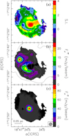 |
Fig. 20 (a) Map (colour image) of the spectral index of the 3 mm continuum emission computed from the emission at the minimum and maximum frequencies observed in the GUAPOS survey. (b) Contour map of the 1 cm continuum emission overlaid on the map of the 3 mm free-free continuum emission calculated using the spectral index information (see text). Contour levels range from 1 to 26 in steps of 5 mJy/beam. (c) Same as panel b, for the 3 mm dust continuum emission. The synthesised beam is shown in the bottom-right corner. |
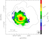 |
Fig. 21 Map of the H2 column density obtained from the dust emission map in Fig. 20c and the temperature map in Fig. 19a. The contours represent the map of the 1 cm continuum emission and are the same as in Fig. 6. The dotted pattern outlines the approximate border of the HMC. The synthesised beam is shown in the bottom-right corner. |
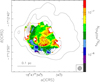 |
Fig. 22 Map of the CH3CCH abundance relative to H2. The contours represent the map of the 1 cm continuum emission and are the same as in Fig. 6. The dotted pattern outlines the approximate border of the HMC. The synthesised beam is shown in the bottom-right corner. |
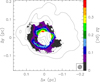 |
Fig. 23 Map of the estimated geometrical thickness of the molecular gas along the line of sight. The RA and Dec axes are expressed in pc to ease the comparison with Δz. The 0,0 position corresponds to the phase centre of the ALMA observations. The contours represent the map of the 1 cm continuum emission and are the same as in Fig. 6. The synthesised beam is shown in the bottom-right corner. |
5.2 Kinematics of the region
it is interesting to compare the velocity field of the molecular gas with that of the ionised gas. First of all, we consider the velocities of the C33S(2-1) and H39α lines with respect to the systemic LSR velocity of the HMC (96.5 km s−1). The corresponding maps are shown in Figs. 24a and 24b. For a more detailed comparison, in Fig. 24c, we plot the difference between the recombination line velocity and the C33 S(2-1) line velocity at the same position. While the ionised gas is red-shifted all over the HII region, with the sole exception of a small area to the SE, the molecular gas is blue-shifted to the south and towards the UC HII region and is close to the systemic velocity over the remaining area. Our hypothesis is that the ionised gas is expanding away from the observer, which in turn suggests that the molecular gas associated with the HMC is located mostly between the HII region and the observer. As for the blue-shifted C33S emission over the southern part of the map in Fig. 24c, it is likely due to overlap with another molecular cloud that (Beltrán et al. 2022b) proposed to be colliding with the cloud containing the HII region and the HMC.
To establish the 3D distribution of the different gas components and thereby confirm our hypothesis that the ionised gas is expanding away from the observer and from the molecular clump enshrouding the HMC, we take advantage of the presence of absorption in the CN(1-0) line. In Fig. 24d, we show the difference between the velocity of the H39α line and that of the absorption dip in the CN line. The map is qualitatively very similar to that in Fig. 24c, which proves that the CN absorption and C33S emission trace the same region. Therefore, since the CN line is seen in absorption, the corresponding gas must be located between the observer and the HII region, with the latter expanding away from the molecular clump in a ‘champagne flow’ (see Yorke 1983 and references therein).
Finally, it is worth analysing the velocity field towards the UC HII region. The inverse P-Cygni profiles of Fig. 7 hints at the existence of residual infall of the surrounding molecular gas. The presence of strong interaction between the molecular and the ionised gas through the eastern border of the UC HII region is witnessed by the kinematics of the ionised component. In Fig. 25 we compare maps of the LSR velocity and FWHM of the H40α line to a map of the 7 mm continuum emission. The peak of the UC HII region is skewed to the east, namely towards the molecular gas, so that the ionised gas has a cometary shape hinting at expansion towards the west. in particular, from Fig. 25a we can see that across the UC HII region the ionised gas has a velocity gradient almost in the same direction as the symmetry axis of the cometary shape (see the dashed line in the figure) and the velocity over the whole UC HII region is red-shifted with respect to that of the HMC (96.5 km s−1 ). Further evidence of interaction between the ionised gas with the molecular cloud is provided by Fig. 25b, where the maximum FWHM of the recombination line is found right at the eastern border of the UC HII region. Noticeably, this is also the location where the electron temperature peaks in Fig. 14a, which lends further support to the existence of strong activity in this area.
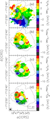 |
Fig. 24 (a) Map of the difference between the velocity of the C33 S(2-1) line and the systemic LSR velocity of the HMC (96.5 km s−1 ). The white contours correspond to 0 km s−1. The black contours are the same as in Fig. 6. The dotted pattern outlines the approximate border of the HMC. (b) Same as panel a, for the difference between the velocity of the H39α line and that of the HMC. (c) Same as panel a, for the difference between the velocity of the H39α line and that of the C33 S(2-1) line. (d) Same as panel a, for the difference between the velocity of the H39α line and that of the absorption dip of the CN(1-0) line. the HMC. The synthesised beam is shown in the bottom-right corner. |
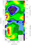 |
Fig. 25 (a) Contour map of the 7 mm continuum emission (enlargement of the map in Fig. 1) overlaid on the H40α velocity map (colour image) of Fig. 4. The dashed line marks the approximate axis of the cometary shaped UC HII region as well as the approximate direction of the velocity gradient across it. (b) Same as panel a, for the line FWHM. The synthesised beams are shown in the bottom left (for the 7 mm map) and right (for the velocity map) corners. |
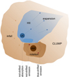 |
Fig. 26 Sketch of the proposed scenario for the G31.41+0.31 star forming region. The dashed lines represent the three lines of sight corresponding to the spectra in Figs. 7–9. The observer is located at the bottom of the figure. |
5.3 A 3D view of the G31.41+0.31 region
Based on the analysis of the previous sections, we propose a tentative 3D picture of the HII region and the molecular clump enshrouding it. In summary, from the previous discussion we conclude that:
The HMC and the lower-density molecular gas have basically the same velocity (Fig. 24a), which suggests that the HMC is lying inside the molecular clump;
The CN absorption feature towards the HII region proves that the medium-density gas lies between the ionised gas and the observer;
The ionised gas (including the UC HII region) is red-shifted with respect to the molecular gas (Figs. 24b and 24c), which proves that the HII region is expanding away from the observer to the NW;
The red-shifted absorption towards the UC HII region (see the inverse P-Cygni profiles in Fig. 7) proves the existence of residual Infall;
The NE-SW velocity gradient across the HMC (Figs. 16b and 17b) is consistent with that observed inside the HMC, which suggests that the lower-density gas enshrouding the HMC could be undergoing rotation too.
With all the above in mind, we propose a scenario that should explain the observed features. This is depicted in Fig. 26. The basic idea is that there are two star formation centres in G31.41+0.31, one associated with the HII region and another, less evolved, associated with the HMC. Both are located inside a molecular clump whose remnant is still clearly visible on the parsec scale at 8 μm (see Fig. 2a), as a dark lane extending to the east and to the south. This medium-density gas is still infalling as witnessed by the red-shifted absorption seen along the line of sight through the UC HII region. The presence of infall is consistent with the scenario proposed by (Beltrán et al. 2022b), where the material is accreting through filaments onto a “hub” where the HII region and HMC are located. The high-density gas more tightly associated with the HMC is rotating, as well as the HMC itself, while the ionised gas is expanding to the NW in a champagne flow receding from the observer. We believe that the HMC lies in front of the HII region, because the medium-density gas is rotating with the HMC and is seen in (slightly red-shifted) absorption (Fig. 8). Moreover, the HMC should not be too far from the HII region surface, because we see an electron density enhancement between the HMC and the SE border of the HII region (see Fig. 14c). This hints at a proximity between the two objects.
6 Summary and conclusions
The present study is part of the GUAPOS project, which observed the G31.41+0.31 HMC and associated UC HII region using the whole bandwidth of the 3 mm ALMA receivers with a 1″.2 angular resolution. We used the data of 15 hydrogen recombination lines and several molecular transitions to investigate the velocity field and physical structure of the ionised and molecular gas. The recombination line maps were fitted with a suitable NLTE model to derive the electron temperature and density all over the HII region, while the same parameters for the molecular gas were obtained from rotation diagrams of the CH3CCH(6-5) line emission. We find that the HII region is expanding to the NW, as suggested also by its cometary shape, while it is pressure-confined to the SE. A comparison between the velocity fields obtained from the recombination and molecular lines suggests that the molecular gas is still undergoing residual infall towards the peak of the UC HII region and is expanding away from it in the southern part. Based on our results, we propose a 3D picture where most of the molecular gas is distributed to the east of the HII region and between the latter and the observer, with the HMC lying close to the interface between the ionised gas and the lower density molecular gas. While, in all likelihood, the HII region is ionisation bound, we believe that due to the cometary shape, a non-negligible fraction of the stellar photons longwards of 912 Å might escape from the surrounding molecular cloud, thus leading to an underestimation of the bolometric luminosity of the region.
Acknowledgements
R.C., M.T.B., and A.L. acknowledge financial support through the INAF Large Grant “The role of MAGnetic fields in MAssive star formation” (MAGMA). C.M. acknowledges funding from the European Research Council (ERC) under the European Union’s Horizon 2020 program through the ECOGAL Synergy grant (ID 855130) and funding from INAF Mini Grants RSN2 2024 “Zodyac” CUP C83C25000340005. V.M.R. and L.C. acknowledge support from the grant PID2022-136814NB-I00 by the Spanish Ministry of Science, Innovation and Universities/State Agency of Research MICIU/AEI/10.13039/501100011033 and by ERDF, UE; V.M.R. also acknowledges the grant RYC2020-029387-I funded by MICIU/AEI/10.13039/501100011033 and by “ESF, Investing in your future”, and from the Consejo Superior de Investigaciones Científicas (CSIC) and the Centro de Astrobiología (CAB) through the project 20225AT015 (Proyectos intramurales especiales del CSIC); and from the grant CNS2023-144464 funded by MICIU/AEI/10.13039/501100011033 and by “European Union NextGener-ationEU/PRTR”. A.S.-M. acknowledges support from the RyC2021-032892-I grant funded by MCIN/AEI/10.13039/501100011033 and by the European Union ‘Next GenerationEU’/PRTR, as well as the program Unidad de Excelencia María de Maeztu CEX2020-001058-M, and support from the PID2023-146675NB-I00 (MCI-AEI-FEDER, UE). A.L.-G. acknowledges support from the grant PID2022-136814NB-I00 by the Spanish Ministry of Science, Innovation and Universities/State Agency of Research MICIU/AEI/10.13039/501100011033 and by ERDF, UE; and from the Consejo Superior de Investigaciones Científicas (CSIC) and the Centro de Astrobiología (CAB) through the project 20225AT015 (Proyectos intramurales especiales del CSIC). The project that gave rise to these results received the support of a fellowship from the “la Caixa” Foundation (ID 100010434). The fellowship code is LCF/BQ/PR25/12110012. This paper makes use of the following ALMA data: ADS/JAO.ALMA#2017.1.00501.S. ALMA is a partnership of ESO (representing its member states), NSF (USA) and NINS (Japan), together with NRC (Canada), NSC and ASIAA (Taiwan), and KASI (Republic of Korea), in cooperation with the Republic of Chile. The Joint ALMA Observatory is operated by ESO, AUI/NRAO and NAOJ. This study is also based on observations made under projects 16A-181 and 23A-066 with the VLA of NRAO. The National Radio Astronomy Observatory is a facility of the National Science Foundation operated under cooperative agreement by Associated Universities, Inc.
References
- Beltrán, M. T., Cesaroni, R., Neri, R., et al. 2004, ApJ, 601, L187 [Google Scholar]
- Beltrán, M. T., Cesaroni, R., Neri, R., et al. 2005, A&A, 435, 901 [Google Scholar]
- Beltrán, M. T., Codella, C., Viti, S., Neri, R., & Cesaroni, R. 2009, ApJ, 690, L93 [Google Scholar]
- Beltrán, M. T., Cesaroni, R., Rivilla, V. M., et al. 2018, A&A, 615, A141 [Google Scholar]
- Beltrán, M. T., Padovani, M., Girart, J. M., et al. 2019, A&A, 630, A54 [Google Scholar]
- Beltrán, M. T., Rivilla, V. M., Cesaroni, R., et al. 2021, A&A, 648, A100 [Google Scholar]
- Beltrán, M. T., Rivilla, V. M., Cesaroni, R., et al. 2022a, A&A, 659, A81 [NASA ADS] [CrossRef] [EDP Sciences] [Google Scholar]
- Beltrán, M. T., Rivilla, V. M., Kumar, M. S. N., Cesaroni, R., & Galli, D. 2022b, A&A, 660, L4 [NASA ADS] [CrossRef] [EDP Sciences] [Google Scholar]
- Beltrán, M. T., Padovani, M., Galli, D., et al. 2024, A&A, 686, A281 [NASA ADS] [CrossRef] [EDP Sciences] [Google Scholar]
- Brocklehurst, M., & Seaton, J. 1972, MNRAS, 157, 179 [NASA ADS] [CrossRef] [Google Scholar]
- Budaiev, N., Ginsburg, A., Barnes, A. T., et al. 2026, ApJ, in press [Google Scholar]
- Benjamin, R. A., Churchwell, E., Babler, B. L., et al. 2003, PASP, 115, 953 [Google Scholar]
- Cesaroni, R., Walmsley, C.M., Kömpe, C., & Churchwell, E. 1991, A&A, 252, 278 [Google Scholar]
- Cesaroni, R., Churchwell, E., Hofner, P., Walmsley, C.M., & Kurtz, S. 1994a, A&A, 288, 903 [Google Scholar]
- Cesaroni, R., Olmi, L., Walmsley, C. M., Churchwell, E., & Hofner, P. 1994b, ApJ, 435, L137 [NASA ADS] [CrossRef] [Google Scholar]
- Cesaroni, R., Hofner, P., Walmsley, C. M., & Churchwell, E. 1998, A&A, 345, 949 [Google Scholar]
- Cesaroni, R., Hofner, P., Araya, E., & Kurtz, S. 2010, A&A, 509, A50 [NASA ADS] [CrossRef] [EDP Sciences] [Google Scholar]
- Cesaroni, R., Beltrán, M.T., Zhang, Q., Beuther, H., & Fallscheer, C. 2011, A&A, 533, A73 [NASA ADS] [CrossRef] [EDP Sciences] [Google Scholar]
- Cesaroni R., Pestalozzi, M., Beltrán, M. T., et al. 2015, A&A, 579, A71 [NASA ADS] [CrossRef] [EDP Sciences] [Google Scholar]
- Cesaroni R., Sánchez-Monge, Á., Beltrán, M. T., et al. 2016, A&A, 588, L5 [NASA ADS] [CrossRef] [EDP Sciences] [Google Scholar]
- Cesaroni R., Sánchez-Monger, Á., Beltrán, M. T., et al. 2017, A&A, 602, A59 [NASA ADS] [CrossRef] [EDP Sciences] [Google Scholar]
- Cesaroni R., Beltrán, M. T., Moscadelli, L., Sánchez-Monger, Á., & Neri, R. 2019, A&A, 624, A100 [NASA ADS] [CrossRef] [EDP Sciences] [Google Scholar]
- Cesaroni, R., Moscadelli, L., Caratti o Garatti, A., et al. 2023, A&A, 680, A110 [NASA ADS] [CrossRef] [EDP Sciences] [Google Scholar]
- Colzi, L., Rivilla, V. M., Beltrán, M. T., et al. 2021, A&A, 653, A129 [NASA ADS] [CrossRef] [EDP Sciences] [Google Scholar]
- Fazio, G. G., Hora, J. L., Allen, L. E., et al. 2004, ApJS, 154, 10 [Google Scholar]
- Fontani, F., Cesaroni, R., Caselli, P., & Olmi, L. 2002, A&A, 389, 603 [NASA ADS] [CrossRef] [EDP Sciences] [Google Scholar]
- Fontani, F., Mininni, C., Beltrán, M. T., et al. 2024, A&A, 682, A74 [NASA ADS] [CrossRef] [EDP Sciences] [Google Scholar]
- Gordon, M. A., & Churchwell, E. 1970, A&A, 9, 307 [Google Scholar]
- Gordon, M. A., & Sorochenko, R. L. 2002, Radio Recombination Lines: Their Physics and Astronomical Applications, Astrophysics and Space Science Library (The Netherlands: Springer), 282 [Google Scholar]
- Immer, K., Li, J., Quiroga-Nuñez, L. H., et al. 2019, A&A, 632, A123 [NASA ADS] [CrossRef] [EDP Sciences] [Google Scholar]
- Lampton, M., Margon, B., & Bowyer, S. 1976, ApJ, 208, 177 [Google Scholar]
- Law, C. Y., Beltrán, M., Furuya, R. S., et al. 2025, A&A, 697, L4 [NASA ADS] [CrossRef] [EDP Sciences] [Google Scholar]
- López-Gallifa, Á., Rivilla, V. M., Beltrán, M. T., et al. 2024, MNRAS, 529, 3244 [CrossRef] [Google Scholar]
- López-Gallifa, Á., Rivilla, V. M., Beltrán, M. T., et al. 2025, A&A, 704, A288 [NASA ADS] [CrossRef] [EDP Sciences] [Google Scholar]
- Lumsden, S. L., Hoare, M. G., Urquhart, J. S., et al. 2013, A&A, ApJS, 208, 11 [Google Scholar]
- McMullin, J. P., Waters, B., Schiebel, D., Young, W., & Golap, K. 2007, ASP Conf. Ser., 376, 127 [Google Scholar]
- Mezger, P. G., & Henderson, A. P. 1967, ApJ, 147, 471 [Google Scholar]
- Mininni, C., Beltrán, M. T., Rivilla, V. M., et al. 2020, A&A, 644, A84 [NASA ADS] [CrossRef] [EDP Sciences] [Google Scholar]
- Mininni, C., Beltrán, M. T., Colzi, L., et al. 2023, A&A, 677, A15 [NASA ADS] [CrossRef] [EDP Sciences] [Google Scholar]
- Molinari, S., Swinyard, B., Bally, J., et al. 2010, PASP, 122, 314 [Google Scholar]
- Panagia, N. 1973, AJ, 78, 929 [NASA ADS] [CrossRef] [Google Scholar]
- Peters, T., Banerjee, R., Klessen, R. S., et al. 2010a, ApJ, 711, 1017 [NASA ADS] [CrossRef] [Google Scholar]
- Peters, T., Mac Low, M.-M., Banerjee, R., Klessen, R. S., & Dullemond, C. P. 2010b, ApJ, 719, 831 [Google Scholar]
- Peters, T., Klessen, R. S., Mac Low, M.-M., & Banerjee, R. 2010c, ApJ, 725, 134 [Google Scholar]
- Rivilla, V. M., Beltrán, M. T., Cesaroni, R., et al. 2017, A&A, 598, A59 [NASA ADS] [CrossRef] [EDP Sciences] [Google Scholar]
- Sánchez-Monge, Á., Beltrán, M.T., Cesaroni, R., et al. 2013, A&A, 550, A21 [NASA ADS] [CrossRef] [EDP Sciences] [Google Scholar]
- Sánchez-Monge, Á., Schilke, P., Ginzburg, A., Cesaroni, R., & Schmiedeke, A. 2018, A&A, 609, A101 [NASA ADS] [CrossRef] [EDP Sciences] [Google Scholar]
- Schuller, F., Menten, K. M., Contreras, Y., et al. 2009, A&A, 504, 415 [NASA ADS] [CrossRef] [EDP Sciences] [Google Scholar]
- Spitzer, L. 1998, “Physical processes in the interstellar medium”, ed. Wiley-VCH [Google Scholar]
- Ungerechts, H., Walmsley, C. M., & Winnewisser, G. 1986, A&A, 157, 207 [Google Scholar]
- Urquhart, J. S., Thompson, M. A., Moore, T. J. T., et al. 2013, MNRAS, 435, 400 [Google Scholar]
- Werner, M., Roellig, T., Low, F., et al. 2004, ApJS, 154, 1 [NASA ADS] [CrossRef] [Google Scholar]
- Wood, D. O. S., & Churchwell, E. 1989a, ApJS, 69, 831 [Google Scholar]
- Wood, D. O. S., & Churchwell, E. 1989b, ApJ, 340, 265 [NASA ADS] [CrossRef] [Google Scholar]
- Wood, D. O. S., & Churchwell, E. 1991, ApJ, 372, 199 [Google Scholar]
- Yorke, H. W., Tenorio-Tagle, G., Bodenheimer, P. 1983, A&A, 127, 313 [Google Scholar]
As already noted in Sect. 3.2, the H54γ line partly overlaps with two of the NS J=5/2→3/2 hyperfine components.
For this purpose we defined the border of the HMC as the 10% contour level of the C33S(2–1) integrated emission, represented by the dotted pattern in Fig. 1.
Appendix A Radius of the HII region
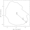 |
Fig. A.1 Sketch of the method adopted to estimate the HII region radius for a generic point P. The contour corresponds to the 5σ level of the 3 mm continuum emission and is assumed to be the border of the HII region, while B is the barycentre of this contour. I is the intersection between the half-line originating in B and passing through P. The segment BI is the radius used in our model calculations to determine the intensity of the hydrogen recombination lines in P. The 0,0 position is the phase centre of the ALMA observations. |
As explained in Sect. 4.1.1, our model assumes that the HII region is spherical and requires knowledge of its radius. Since the G31.41+0.31 HII region is far from an ideal sphere, we decided to estimate a value of the radius that depends on the position. In Fig. A.1 we show a sketch that illustrates our approach. We assume that the border of the HII region coincides with the 5σ contour level of the 3 mm continuum emission and the HII region centre is taken as the barycentre, B, of such a contour, whose coordinates are
 (A.1)
(A.1)
 (A.2)
(A.2)
with i indicating a generic point of the border and N is the number of these points. For a generic point, P, of the HII region we assume that the HII region radius to be used as an input for our model is equal to the segment BI that connects the centre, B, with the intersection, I, between the HII region border and the half-line originating in B and passing through P. Obviously, this definition implies that the radius varies with P but we believe that this mirrors the irregular shape of the HII region more reliably than approximating the HII region with a sphere of a given radius. The values of the radius obtained in this way range from 3″.8 to 7″.6.
All Tables
Parameters of molecular lines used to study the extended molecular cloud enshrouding the HII region.
All Figures
|
Fig. 1 (a) Maps of the 1 cm (colour image and white contours) and 7 mm (black contours) continuum emission imaged with the VLA. The contour levels of the 1 cm map are drawn in the colour scale to the right, while those of the 7 mm map range from 0.08 to 1.88 in steps of 0.3 mJy/beam. The black dotted pattern outlines the approximate border of the HMC (see text). The dashed rectangle frames the region shown in panel b. The synthesised beams (1″.2 at 1 cm and 0″.21×0″.17 with PA −0°.5 at 7 mm) are shown in the bottom-left and -right corners. (b) Enlargement of the region that contains the UC HII region and the HMC, corresponding to the dashed rectangle in panel a. The symbols have the same meaning as in panel a, with the exception of the colour image that shows the 7 mm continuum emission. We note that the colour scale is saturated (the peak emission at 7 mm is 1.96 mJy/beam) to emphasise the structure of the UC HII region. (c) Contour map of the 3 mm continuum emission obtained from the ALMA data overlaid on the same 1 cm continuum image as in panel a. Contour levels range from 0.5 to 180 mJy/beam in ten logarithmic steps. The synthesised beam (1″.2) is the same for both maps and is shown in the bottom-right corner. |
| In the text | |
|
Fig. 2 (a) Overlay of the 1 cm map of Fig. 1 (contours) and the 8 μm image from the Spitzer/GLIMPSE database (colour image). Contour levels range from 1 to 28 in steps of 9 mJy/beam. The angular resolution of the latter image is shown in the bottom-right corner. The dotted rectangle outlines the region shown in Figs. 1a and c. (b) Same as panel a, for the 70 μm image obtained from the Herschel/Hi-GAL survey. |
| In the text | |
|
Fig. 3 Maps of the integrated emission over the hydrogen recombination lines indicated in the top right corner of each panel. The emission from the HMC is not plotted because the recombination lines are heavily blended with stronger molecular transitions. The circle in the bottomright corner is the synthesised beam. The offsets are relative to the phase centre of the ALMA observations. The emission of the H54γ line is contaminated by two hyperfine components of the NS J = 5/2 → 3/2 transition. |
| In the text | |
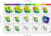 |
Fig. 4 Same as Fig. 3, but for the peak velocity of the recombination lines. |
| In the text | |
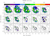 |
Fig. 5 Same as Fig. 3, but for the full width at half maximum of the recombination lines. |
| In the text | |
|
Fig. 6 Contour map of the 1 cm continuum emission overlaid on a map of the peak emission in the H13CO+(1-0) line (grey scale). Contour levels range from 1 to 28 in steps of 3 mJy/beam. The crosses and corresponding labels denote the four template positions that the spectra of Figs. 7–10 have been taken towards. |
| In the text | |
|
Fig. 7 Spectra of various molecular lines (as indicated in each panel) observed towards the UCHII position in Fig. 6 with ICRS coordinates 18h47m34s.555-01° 12′43″.20. The blue dotted and red dashed lines mark, respectively, the systemic LSR velocity of the HMC (96.5 km s−1; Cesaroni et al. 2011) and the peak velocity of the H39α recombination line measured at the given position. |
| In the text | |
|
Fig. 8 Same as Fig. 7 but for the HII position in Fig. 6 with ICRS coordinates 18h47m34s.415-01°12′46″.95. |
| In the text | |
|
Fig. 9 Same as Fig. 7 but for the SW position in Fig. 6 with ICRS coordinates 18h47m34s.245-01°12′50′.25. |
| In the text | |
|
Fig. 10 Same as Fig. 7, but for the S position in Fig. 6 with ICRS coordinates 18h47m34s.415-01°12′51″.30. |
| In the text | |
|
Fig. 11 Maps of the electron temperature obtained from the hydrogen recombination lines indicated in the top right corners of the panels, under the LTE approximation. The offsets are relative to the phase centre of the ALMA observations. The contours are the map of the 3 mm continuum emission shown in Fig. 1c, with contour levels ranging from 1.15 to 28.75 in steps of 4.6 mJy/beam. The synthesised beam is shown in the bottomright corner. |
| In the text | |
|
Fig. 12 Plot of the χ2 computed from Eq. (3) as a function of electron temperature and density at the peak position of the UC HII region. The white dot marks the minimum and the white contour corresponds to the 1σ confidence level. |
| In the text | |
|
Fig. 13 Spectra of the hydrogen recombination lines observed towards the peak of the UC HII region. The name of the line is indicated in the top right corner of each panel. The velocity is relative to the peak velocity of each spectrum, obtained with a Gaussian fit. The red and green curves are the model spectra obtained by fitting only the H39α, H40α, and H41α lines. The H54γ line is contaminated by emission from a molecular line. |
| In the text | |
|
Fig. 14 (a) Map of electron temperature of the HII region, obtained by fitting the hydrogen recombination lines with our model (see text). (b) Map of the relative error on the electron temperature. (c) Same as panel a, for the electron number density. (d) Same as panel b, for the electron number density. The angular resolution is represented by the circle in the bottom-right corner. |
| In the text | |
|
Fig. 15 Spectra of the CH3CCH(6-5) transition towards the four positions marked in Fig 6. The K=0-5 components are indicated by the red dotted lines and labelled accordingly. |
| In the text | |
|
Fig. 16 (a) Map of the opacity of the main hyperfine transition of C33S(2-1) (colour image). The contour map represents the 3 mm continuum emission and is the same as in Fig. 1c. (b) Same as panel a, for the LSR velocity. (c) Same as panel a, for the line FWHM. The synthesised beam is shown in the bottom-right corner. |
| In the text | |
|
Fig. 17 (a) Map of the integrated intensity over the K=0 and 1 components of the CH3CCH(6-5) line (colour image). The contour map represents the 3 mm continuum emission and is the same as in Fig. 1c. (b) Map of the LSR velocity of the CH3CCH(6-5) line obtained by fitting all the K components (see Sect. 4.2.2). (c) Same as panel b, for the line FWHM. The synthesised beam is shown in the bottom-right corner. |
| In the text | |
|
Fig. 18 (a) Map (colour image) of the absolute value of the minimum (negative) brightness temperature of the N = 1-0, J =1/2-1/2, F=3/2-3/2 hyperfine component of the CN(1-0) line. (b) Map of the LSR velocity at which the minimum brightness shown in panel a is attained. The synthesised beam is shown in the bottom-right corner. The contour map represents the 3 mm continuum emission and is the same as in Fig. 1c. |
| In the text | |
|
Fig. 19 (a) Map (colour image) of the rotational temperature obtained from the rotation diagram of the CH3CCH molecule. Contours represent the same map of the 3 mm continuum emission as in Fig. 1c. (b) Map of the relative error on the rotation temperature. (c) Same as panel a, for the CH3CCH column density. (d) Same as panel b, for the CH3CCH column density. The synthesised beam is shown in the bottom-right corner. |
| In the text | |
|
Fig. 20 (a) Map (colour image) of the spectral index of the 3 mm continuum emission computed from the emission at the minimum and maximum frequencies observed in the GUAPOS survey. (b) Contour map of the 1 cm continuum emission overlaid on the map of the 3 mm free-free continuum emission calculated using the spectral index information (see text). Contour levels range from 1 to 26 in steps of 5 mJy/beam. (c) Same as panel b, for the 3 mm dust continuum emission. The synthesised beam is shown in the bottom-right corner. |
| In the text | |
|
Fig. 21 Map of the H2 column density obtained from the dust emission map in Fig. 20c and the temperature map in Fig. 19a. The contours represent the map of the 1 cm continuum emission and are the same as in Fig. 6. The dotted pattern outlines the approximate border of the HMC. The synthesised beam is shown in the bottom-right corner. |
| In the text | |
|
Fig. 22 Map of the CH3CCH abundance relative to H2. The contours represent the map of the 1 cm continuum emission and are the same as in Fig. 6. The dotted pattern outlines the approximate border of the HMC. The synthesised beam is shown in the bottom-right corner. |
| In the text | |
|
Fig. 23 Map of the estimated geometrical thickness of the molecular gas along the line of sight. The RA and Dec axes are expressed in pc to ease the comparison with Δz. The 0,0 position corresponds to the phase centre of the ALMA observations. The contours represent the map of the 1 cm continuum emission and are the same as in Fig. 6. The synthesised beam is shown in the bottom-right corner. |
| In the text | |
|
Fig. 24 (a) Map of the difference between the velocity of the C33 S(2-1) line and the systemic LSR velocity of the HMC (96.5 km s−1 ). The white contours correspond to 0 km s−1. The black contours are the same as in Fig. 6. The dotted pattern outlines the approximate border of the HMC. (b) Same as panel a, for the difference between the velocity of the H39α line and that of the HMC. (c) Same as panel a, for the difference between the velocity of the H39α line and that of the C33 S(2-1) line. (d) Same as panel a, for the difference between the velocity of the H39α line and that of the absorption dip of the CN(1-0) line. the HMC. The synthesised beam is shown in the bottom-right corner. |
| In the text | |
|
Fig. 25 (a) Contour map of the 7 mm continuum emission (enlargement of the map in Fig. 1) overlaid on the H40α velocity map (colour image) of Fig. 4. The dashed line marks the approximate axis of the cometary shaped UC HII region as well as the approximate direction of the velocity gradient across it. (b) Same as panel a, for the line FWHM. The synthesised beams are shown in the bottom left (for the 7 mm map) and right (for the velocity map) corners. |
| In the text | |
|
Fig. 26 Sketch of the proposed scenario for the G31.41+0.31 star forming region. The dashed lines represent the three lines of sight corresponding to the spectra in Figs. 7–9. The observer is located at the bottom of the figure. |
| In the text | |
|
Fig. A.1 Sketch of the method adopted to estimate the HII region radius for a generic point P. The contour corresponds to the 5σ level of the 3 mm continuum emission and is assumed to be the border of the HII region, while B is the barycentre of this contour. I is the intersection between the half-line originating in B and passing through P. The segment BI is the radius used in our model calculations to determine the intensity of the hydrogen recombination lines in P. The 0,0 position is the phase centre of the ALMA observations. |
| In the text | |
Current usage metrics show cumulative count of Article Views (full-text article views including HTML views, PDF and ePub downloads, according to the available data) and Abstracts Views on Vision4Press platform.
Data correspond to usage on the plateform after 2015. The current usage metrics is available 48-96 hours after online publication and is updated daily on week days.
Initial download of the metrics may take a while.