| Issue |
A&A
Volume 710, June 2026
|
|
|---|---|---|
| Article Number | A7 | |
| Number of page(s) | 15 | |
| Section | The Sun and the Heliosphere | |
| DOI | https://doi.org/10.1051/0004-6361/202659635 | |
| Published online | 28 May 2026 | |
Statistical study of Balmer continuum enhancement in solar flares
Astronomical Institute of the University of Bern, Sidlerstrasse 5, 3012 Bern, Switzerland
★ Corresponding author: This email address is being protected from spambots. You need JavaScript enabled to view it.
Received:
27
February
2026
Accepted:
7
April
2026
Abstract
Context. Identifying the physical mechanisms of continuum emission in solar flares is important for improving our understanding of energy transport in the chromosphere. This requires reliable detection of enhanced continuum emission across different flare classes.
Aims. This study aims to quantify the occurrence statistics and spatial and temporal characteristics of near-ultraviolet (NUV) continuum enhancements across various classes of solar flares.
Methods. We analyzed 234 IRIS flare observations and developed two independent detection pipelines. Both pipelines initially extracted candidate enhancement events from pixel-level NUV time series and subsequently eliminated false positives by using the temporal and spatial correspondence between NUV and FUV continuum enhancement. For one of the pipelines, we used Gaussian process regression to quantify the uncertainty in the enhancement magnitudes.
Results. We detect NUV continuum enhancements in 80 out of 234 flares. These enhancements occurred predominantly on the flare ribbon edges and during the GOES impulsive phase, as well as after the GOES peak flux. In a few cases (4 pixels), NUV and FUV continuum enhancements were detected 7−15 minutes before the GOES start or more than 20 minutes after the peak, appearing as indistinct bright points in the active regions. Despite large uncertainties for C-class events, enhancement magnitudes increase with flare class, with X-class flares showing the strongest enhancement.
Conclusions. Our analysis reveals that the enhancements are confined to localized regions on the flare ribbon edges. In terms of flare energetics, this suggests that enhancements may occur in the regions with freshly reconnected magnetic field lines, or in ribbon fronts with gradual and modest high-energy flux injection by non-thermal electrons. Enhancements found significantly after the flare peak in strong flares further suggest multiple heating episodes. The enhancement strengths of flare events as weak as C1.1 from this study serve as an important constraint for flare simulation models.
Key words: Sun: chromosphere / Sun: flares / Sun: UV radiation
© The Authors 2026
 Open Access article, published by EDP Sciences, under the terms of the Creative Commons Attribution License (https://creativecommons.org/licenses/by/4.0), which permits unrestricted use, distribution, and reproduction in any medium, provided the original work is properly cited.
This article is published in open access under the Subscribe to Open model. This email address is being protected from spambots. You need JavaScript enabled to view it. to support open access publication.
1. Introduction
In stark contrast to the relatively stable photosphere, the chromosphere and corona host highly energetic phenomena, one of which are solar flares. The energy released during flares can be detected throughout the electromagnetic spectrum, with a significant fraction emitted in ultraviolet (UV), especially in the form of continuum radiation (Milligan & McElroy 2013). Despite being a significant portion of the flare energy budget, the exact energetics and physical mechanisms of continuum emission are still under debate.
In the late 20th century, flares showing excess emission in visible wavelengths relative to the quiescent solar spectrum were termed white-light flares (WLFs; Najita & Orrall 1970; Hudson 1972). Although initially thought to be rare, later statistical studies based on full-disk solar fluxes suggested that WLFs may be more common. For example, Kretzschmar (2011) concluded that the majority of flares show some level of white-light emission. These enhancements are not confined to the optical range; continuum brightening has also been detected in the UV and infrared (IR) regimes and, for a few cases, found to be temporally correlated with soft and hard X-ray (HXR) emission observed by instruments such as GOES, RHESSI, and Fermi-GBM (Kleint et al. 2016; Joshi et al. 2021). With improved spatial and temporal resolution, a few studies (Heinzel & Kleint 2014; Zuccarello et al. 2020; Joshi et al. 2021) have demonstrated the detectability of near-UV (NUV) continuum enhancements in specific flare occurrences using the Interface Region Imaging Spectrograph (IRIS; De Pontieu et al. 2014). Notably, for a strong flare, Kleint et al. (2016) found that NUV enhancements were stronger than those in the visible or IR and that HXR sources and the locations of NUV continuum enhancement overlap, suggesting that the emission arises at flare footpoints where energy deposition occurs. However, the general occurrence and variability of these enhancements across different flare classes remain poorly understood. In contrast to the relatively extensive statistical investigations of WLFs, no study has attempted to quantify the prevalence of NUV continuum enhancements and their dependence on flare properties.
To derive robust statistics on NUV continuum enhancements across flare classes, the reliability of detection methods is crucial. In the visible range, white-light continuum enhancements were historically observed only in the most energetic flares (M- and X-classes). Only recently have such enhancements been detected in lower-energy flares, including those of C-class intensity (Jess et al. 2008; Castellanos Durán & Kleint 2020; Cai et al. 2024). Detection techniques range from image differencing to intensity thresholds.
But these methods may fail to identify anomalous behaviors, such as enhancements occurring prior to flare onset, because they further rely on assumed temporal or spatial correlations. In this study we alleviate some shortcomings of the detection techniques used previously by applying outlier detection on NUV and far-UV (FUV) data paired with Gaussian process regression (GPR). Gaussian process regression is highly adaptable to individual time series and provides detection significance. This approach removes biases introduced, for instance, through thresholding or clustering criteria.
The physical mechanisms responsible for continuum enhancement remain under debate. In the visible range, proposed explanations include photospheric back-warming (Allred et al. 2005; Machado et al. 1989), Alfvén wave pulses (Xu et al. 2025), direct particle precipitation to the photosphere (Najita & Orrall 1970), recombination to hydrogen level n = 3 producing Paschen continuum enhancement below the Paschen limit at 820 nm, and thermal bremsstrahlung, although the latter does not explain the observed EUV and soft X-ray emission (Neidig 1989). Some of these mechanisms suggest the need for energy transport into the lower solar atmosphere. In the NUV, hydrogen recombination following electron beam bombardment is considered the dominant mechanism, suggesting that emission forms primarily in the chromosphere (Heinzel et al. 2016). Kowalski et al. (2017) carried out radiative hydrodynamic simulations for a strong (X1.0) flare. Their results indicate that enhanced NUV continuum radiation originates from the layers hosting impulsively generated downflows, identified as the chromospheric condensation (CC) layer, along with a heated stationary layer situated beneath this CC layer. This further strengthens the claim that the NUV emission ultimately originates from hydrogen recombination to the n = 2 orbital level (Balmer continuum below the 364.6 nm Balmer limit) as the dominant mechanism.
The FUV continuum, by contrast, may involve contributions from UV line irradiance from the upper chromosphere and the transition region in order to photoionize silicon atoms near the temperature minimum region (Doyle & Phillips 1992). An in-depth understanding of the physical origin of continuum enhancement for different flare energies ultimately requires flare simulations.
In this study, we investigated the occurrence and variability of NUV (Balmer) continuum enhancements using 234 IRIS NUV and FUV flare observations of varying classes. By employing detection techniques that do not rely on coincident HXR signals or strict threshold constraints, we aim to characterize continuum enhancements in a less constrained manner. The paper is structured as follows. Section 2 describes the dataset, selection criteria, and detection methodology. Section 3 presents the statistical results, and Section 4 discusses the effects on flare energetics.
2. Observations and methods
2.1. Observations
2.1.1. IRIS
IRIS is a UV imaging spectrograph that captures images and spectra of the Sun. This study utilized IRIS Level-2 NUV spectral observations, which are calibrated for darks, flatfield, geometric corrections, wavelength, and spatial alignment.
The Slit-Jaw Imager (SJI) on board IRIS captures broadband images of the solar surface in the FUV (1335 Å and 1400 Å, each with a 40 Å bandpass) and NUV (2796 Å and 2831 Å, each with a 4 Å bandpass) with a field of view of 175″ × 175″. The spectrograph consists of a single  -wide slit that observes the solar surface in the FUV (1331.7−1358.4 Å and 1389.0−1407.0 Å, with a 26 mÅ spectral resolution) and the NUV (2782.7−2835.1 Å, with a 53 mÅ spectral resolution), scanning a region in steps if the observation is not in sit-and-stare mode.
IRIS operates with “line lists” that define which part of the spectrum to record. The flare line list, which contains several NUV “continuum” windows, is most commonly used for flare observation programs.
The flare observations for this study were selected using the Google document flare list1 maintained by the IRIS team. Observations with a large number of raster positions enhance the spatial sampling of the active region. However, this comes at the cost of reduced temporal resolution. To balance these factors, we restricted our analysis to observations with sixteen or fewer raster positions. Additionally, we excluded limb flares (heliocentric angle μ < 0.4) to avoid underestimating flare intensities. Extended emission near the limb may appear artificially fainter if a part of the emission originates in deeper layers or suffers from projection effects.
Applying the constraints on the raster count, heliocentric angle, and the availability of the continuum wavelengths used in this study results in a dataset comprising 385 flare instances. To determine the number of flares where the ribbon intersects the IRIS slit, we conducted a manual inspection of IRIS SJI images sampled at three-minute intervals throughout the GOES-reported flare duration. We obtained a final dataset of 234 flare instances from 3 February 2014 to 10 March 2024. This dataset includes 34 B-class, 150 C-class, 39 M-class, and 11 X-class flares. Lastly, we preprocessed the spectral data using a pipeline described in Zbinden et al. (2024), which removes overexposed pixels (i.e., those with overexposure of at least 3 wavelength points) and pixels with missing signals (i.e., with negative values).
2.1.2. GOES
The Geostationary Operational Environmental Satellite (GOES) is a collection of geostationary satellites designed to monitor the space environment and meteorological phenomena. Since the launch of the first satellite, GOES-1, in 1975, a total of 19 satellites have been placed in orbit, with GOES 18 and 19 currently (as of 2026) in operation. The GOES satellites provide soft X-ray solar measurements in a long channel (1−8 Å) and a short channel (0.5−4 Å), with a temporal resolution of 1 s. The X-ray fluxes from GOES 8−15 were historically scaled to match the older satellites. However, it was later realized that the sensors on these satellites were already accurate and that this scaling was unnecessary. To recover the true fluxes for flares observed by these satellites, it is recommended in the GOES XRS document2 that the short-channel flux be divided by a factor of 0.85 and the long-channel flux by 0.7. The flare classes available from NOAA archival data for these older events, however, are still based on the scaled fluxes, introducing minor discrepancies in flare strength when comparing data from GOES 8–15 (pre-2020) with that from newer satellites. We therefore used the data as follows: scaled fluxes and corresponding flare classes for events before 2020, and “true” (unscaled) fluxes with their corresponding flare classes for events after 2020. While this introduces some complexity when comparing pre- and post-2020 flares, the scientific interpretation of our results remains unaffected, particularly because our pipeline only detected eight flares showing NUV continuum enhancements after 2020.
2.2. Methods
Defining a continuum range in the NUV spectrum can be challenging due to spectral lines that contaminate the continuum, producing a pseudo-continuum. Figure 1 illustrates the continuum windows chosen for our study, the same continuum windows defined by Heinzel & Kleint (2014). The two narrow windows were selected to avoid contamination by spectral lines.
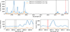 |
Fig. 1. Observed Mg II h and k spectrum, with the continuum windows used in this study (vertical dashed lines). The continuum windows are located far from the wings of the strong resonant Mg II lines at 2796 and 2803 Å. Bottom: Magnified views of the selected continuum regions. The blue spectrum corresponds to the time when the continuum emission was enhanced, while the orange spectrum represents the post-enhancement period during the flare’s impulsive phase. |
This continuum is not free from spectral contamination; it contains a “forest” of spectral lines, most of which are not strong lines. One of the windows is 2825.7 − 2825.8 Å (called 2826 in the following sections), while the other is 2832.1 − 2832.16 Å (denoted 2832). With this definition, one can characterize an event of continuum enhancement when there is “impulsive” emission in the NUV continuum. An example is presented in Fig. 2. The figure shows a steep intensity increase, occurring simultaneously in the continuum and a spectral line. Figure 3 shows the corresponding broadband continuum emission (Kleint et al. 2017) in the center-right of the 2832 Å slit-jaw image. To identify such events, we constructed pixel-wise time series as follows. IRIS observations often span several hours, during which satellite drift can introduce spatial mixing, producing artificial variations in the time series. In addition, persistent bright points vary on longer timescales and may therefore contribute to gradual intensity fluctuations in the time series. Superimposed on these are shorter-timescale intensity fluctuations arising from photospheric granulation, which typically evolves over a characteristic timescale of 5−10 minutes (Hirzberger et al. 1999). As a result, pixel-level time series show a rich diversity of variability. To mitigate the impact of spatial drift and capture granular variations on several characteristic timescales, we extracted a 30-minute segment from each time series, ideally beginning 25 minutes before and ending 5 minutes after the peak time of GOES. If the GOES peak occurred too close to the start or end of the observation, we adjusted this window to maintain a total duration of approximately 30 minutes. We then tested two independent pipelines to detect continuum enhancements, estimate the pre-flare continuum level, and quantify the associated uncertainty in the enhancement magnitude. A flowchart summarizing the steps of each pipeline is shown in Fig. 4. The two pipelines are described separately below.
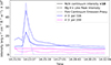 |
Fig. 2. Impulsive increase observed in the NUV continuum (2826 Å window; solid line), the peak intensity of the Mg II k line (dashed line), and the FUV continuum emission proxy (dotted line) at pixel (pxl) 316 (blue), raster position (rr) 3, during an X-class flare on 27-10-2014 at 14:23:12. In contrast, no such behavior is seen in the time series of other pixels on the same raster position, such as pixel 200 (pink line). Refer to Fig. 3 for the SJI image. |
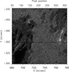 |
Fig. 3. Slit-jaw image in the 2832 Å continuum window of an active region during a solar flare, showing enhanced NUV continuum emission near the center right. The SJI observation time was 27-10-2014 at 14:23:16.950. |
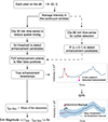 |
Fig. 4. Flowchart of the methodology used in this study, highlighting the differences in outlier detection and uncertainty estimation between the intensity threshold and IF approaches. The letter ‘c’ refers to the contamination parameter, which controls the proportion of detected outliers. GPR is used for uncertainty estimation (see Sect. 2.2.3 for details). |
2.2.1. Continuum enhancement detection using intensity thresholds
In the 2014-03-29 X-class flare, previously analyzed in detail by Kleint et al. (2016), strong NUV (Heinzel & Kleint 2014) and FUV continuum enhancements were observed on the flare ribbons. Building on this, we examined all visually confirmed cases of NUV continuum enhancement in that event and found that they were consistently accompanied by simultaneous FUV continuum enhancements (appearing as bright bands when viewed in the pixel vs. wavelength visualization for any particular timestamp) at the same spatial locations and time. We therefore tested this FUV signature on a subset of flares to evaluate its reliability as a necessary condition for detection in our automated pipeline. This filter was not intended to rule out the physical possibility of FUV-only enhancements, but rather to reduce false positives–i.e., apparent NUV enhancements that are not associated with energy deposition during a flare. This approach offers two advantages. First, it eliminates the need to assume specific spatial or temporal clustering properties of the enhancement, allowing us to detect anomalies in this behavior (e.g., identifying potential continuum enhancements occurring before the flare onset). Second, FUV enhancement is significantly easier to detect due to its higher contrast compared to NUV enhancement, as granulation signals are not strong in the FUV spectrum. To evaluate our method, we tested it on a subset of three flares with the following IRIS observation IDs: X-class flare at 14:04:20 20141027_140420_3860354980, M-class flare at 01:38:49 20141021_181052_3860261353, and C-class flare at 17:32:00 20141019_145935_3860354980. In this sample of three flares (X-, M-, and C-class), all visually confirmed instances (above 3σ) of NUV continuum enhancement were accompanied by co-temporal and co-spatial FUV continuum brightening. Moreover, all NUV-enhanced pixels with corresponding FUV enhancements were located on the flare ribbon and occurred within the GOES flare time for our flare subset. An example is shown in Fig. 2, where one can notice the co-temporal behavior of the NUV-FUV continuum enhancement.
Our NUV continuum enhancement detection pipeline begins by first detecting enhancement candidates in the NUV continuum time series, followed by a filtering step that retains only those events that coincide with FUV continuum brightening. One could, of course, reverse the process and start with FUV detections. However, this would either lead to more false positives in the NUV or would make it harder to confirm the associated NUV enhancement because granulation noise is stronger in the NUV.
For the NUV continuum time series, we detected enhancements in individual time series rather than applying a global threshold. This choice is based on the observation that different pixels show varying levels of continuum variation, as also observed by Cai et al. (2024). To identify potential enhancement candidates, we detected outliers exceeding three standard deviations in each individual NUV continuum pixel time series. We considered a pixel a potential enhancement candidate if it exhibited a three sigma deviation in both the NUV continuum windows. We subsequently developed a method to detect FUV enhancements. Since detecting relative enhancements in the FUV (1352.30 − 1355.83 Å) does not require knowledge of the absolute continuum level, we did not define a fixed continuum window. Instead, we selected 50 equally spaced wavelength points in the FUV spectrum and classified a pixel as exhibiting FUV continuum enhancement if its signal exceeded a threshold relative to other pixels at a given timestamp. Specifically, we considered a pixel enhanced if its intensity surpassed “n” times the interquartile range (IQR) above the third quartile at more than “m” wavelength points, effectively identifying bright bands in the FUV spectrum. Our IQR-based approach requires selecting two parameters: the threshold “n” for outlier detection and the number of wavelength points “m”, where the pixel must meet the threshold condition to be classified as showing continuum enhancement. As shown in Fig. 5 (right panel), spectral emission near 1354.07 and 1355.8 Å easily satisfies m ≈ 20. Accounting for other potential strong spectral lines, we found m = 35 to be neither too high nor too restrictive for detecting continuum enhancements, as there was no significant difference between detection counts for m = 25 and m = 35. However, setting m = 45 was too stringent for detecting bright bands. Additionally, reducing the IQR threshold did not increase the number of detections, suggesting that further FUV detections were limited by the available NUV enhancement candidates. Based on these findings, we adopted a threshold of 1.5 IQR above the third quartile and set m = 35 as the criterion for detecting FUV continuum enhancement. Once a candidate passed the FUV criterion, the magnitude of NUV enhancement was calculated by subtracting the average of the NUV pre-flare continuum time series from the enhanced value.
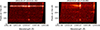 |
Fig. 5. Example of continuum emission in FUV, corresponding to the timestamp of enhanced continuum emission seen in NUV (refer to Fig. 2). Right: Example timestamp, with no continuum emission above our threshold. The vertical brown markers along the x-axis indicate the 50 equally spaced wavelength points used in defining the FUV bright-band detection criterion. |
2.2.2. Continuum enhancement detection using Isolation Forest
The previously described method detects continuum enhancements based on 3σ deviations in NUV time series and simultaneous FUV emission. However, this approach may miss additional valid events since outlier candidates are marked based on the assumption that the intensity across time is normally distributed. To overcome this limitation, we introduced an algorithm based on machine learning that identifies “deviations” in time series and thereby expands the list of potential enhancement candidates.
We used the unsupervised Isolation Forest (IF) algorithm (Liu et al. 2012), which does not assume any specific underlying distribution about the NUV continuum time series. The algorithm works by
-
randomly selecting a feature (in this case, intensity values in the NUV time series, since this is a univariate time series);
-
splitting the data along a randomly chosen threshold for that feature;
-
repeating this process recursively, isolating each data point from the rest of the dataset.
As illustrated in Fig. 6, the IF algorithm identifies not only peaks but also valleys and other distinct features. Despite detecting some irrelevant outliers (i.e., features other than peaks), we find that, with the exception of fewer than five time series, all enhancements found by IF that additionally pass the FUV filtering condition occur within the GOES flare event interval and on the flare ribbon. Moreover, we can eliminate insignificant detections when their uncertainties are quantified using GPR, as discussed in the following paragraphs. We note that the length of the time series fed to the IF algorithm for outlier detection was increased to 1 hour. This was done in order to improve the uncertainty quantification performance of GPR discussed in Sect. 2.2.3. In the IF algorithm, outliers are identified on the basis of how easily the data points are isolated during the recursive partitioning process.
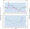 |
Fig. 6. Comparison between outlier detections, using the three-sigma threshold (blue-shaded region) around the mean (horizontal solid black line) and IF with a contamination parameter of 0.1. The colored points are outlier candidates detected by IF, and the red points are true positive enhancements filtered by detecting corresponding FUV continuum emission. Top: 2014-10-22 M-class flare with the IF accurately detecting the rising and decay phase of the enhancement. Bottom: 2014-03-29 X-class flare, with the IF detecting enhancements in cases where a simple intensity threshold would fail. The dotted blue curve represents the GOES flux. The dotted magenta curve represents the time derivative of the 3 s averaged GOES flux (arbitrarily scaled), often used as a proxy signature of nonthermal processes. |
Data points that require fewer splits are deemed anomalous. The proportion of points classified as outliers is controlled by the contamination parameter (c), which defines the expected fraction of anomalies in the dataset. Higher contamination values result in more detected anomalies, while lower values constrain detections to the most extreme outliers. We adopted a contamination value of 0.1, corresponding to 10% of each time series classified as outliers. This choice was motivated by a comparative assessment of the IF’s performance against simple intensity threshold-based methods. When the contamination parameter was set to 0.05, IF yielded results comparable to those obtained using intensity thresholds. For a value higher than 0.1, IF heavily categorized inherent variations as outliers. A selection of example time series, shown in Fig. 6, demonstrates how IF more reliably captures the rise or decay phases of enhancements compared to static thresholds. Once anomalous points are detected in NUV, they are passed through the FUV filter to confirm the case of enhancement.
Since enhancements are detected on granulation variation scales, it is essential to estimate the underlying granulation baseline. This baseline represents the continuum intensity in the absence of enhancement and serves as the pre-flare level from which the magnitude of the observed enhancement can be derived. When the detection algorithm identifies enhancement in a pixel-level time series, a short temporal segment (5 min, centered on the detected enhancement) is excluded from the time series to avoid contamination by flare-related emission. The remaining data are then used to construct the baseline.
Rather than defining a single fixed baseline value, the reconstructed baseline provides a time-dependent estimate of the continuum intensity in the absence of enhancement, such that each enhanced timestamp has a corresponding baseline value. The enhancement magnitude is computed as the difference between the observed intensity and this baseline value. While linear interpolation could, in principle, be used to estimate the baseline (Castellanos Durán & Kleint 2020), it does not provide a time-dependent uncertainty estimate. In contrast, the algorithm we employed, GPR (Rasmussen 2004), provides both a baseline prediction and an uncertainty estimate that adapts to the local variability of the granulation signal rather than assuming a constant uncertainty derived from the global standard deviation of the time series. We refer the reader to Rasmussen (2004) for a detailed introduction to the algorithm and its mathematical background. We only briefly introduce the idea behind the algorithm here.
Gaussian process regression is a regression model popular for its ability to provide confidence intervals for each point-prediction. This regression algorithm does not simply fit an a priori known functional form to the data. Instead, it provides a probability distribution of many potential functions. These functions are characterized using a kernel, which essentially is a mathematical formula that outputs the covariance between data points. The prior probability distribution over the functions, errors, and uncertainties are then assumed to follow a Gaussian distribution. The kernel choice can be guided by prior information about the data. Once selected, the log marginal likelihood of observing the data points can be calculated and maximized to find the optimal hyperparameters associated with the kernel. Predictions can then be made using the conditional properties of Gaussian distributions. To model the NUV continuum granulation time series, we used the prior knowledge that granulation signals are stochastic in nature and have a characteristic timescale. Two kernels are popular to model processes that follow a characteristic length scale: the Matern and radial basis function (RBF) kernel. We tested both and added a white noise kernel to model any stochastic behavior in the intensity. The lower bound of the length scale was set to a value twice the cadence of the respective observation, and the higher bound was set to five times the cadence, as a single test observation showed that smaller length scales perform better. We discuss more details of the evaluation of the algorithms’ capability to provide prediction intervals in the next section.
2.2.3. Uncertainty estimation
For enhancement detection based on intensity thresholds, the uncertainty in the NUV continuum enhancement magnitude is estimated using the 3σ value computed from the time series itself. In contrast, for enhancements identified using the IF algorithm, the probabilistic nature of the GPR model provides prediction intervals for each point along the predicted baseline during the enhancement period. To evaluate the uncertainty quantification performance of the algorithm, we constructed an observation set comprising a mix of active regions both with and without flare events. We first excluded any pixels with continuum enhancements using the IF, followed by the FUV filtering approach, and also ensured that no major cosmic ray events were present in these observations.
This step is crucial, as spurious peaks caused by cosmic rays or continuum enhancements are unpredictable by our model and may appear in the test set, thus degrading model performance. It is important to note, however, that the presence of cosmic ray events does not affect the detection of continuum enhancement events themselves.
As mentioned earlier, we extended the total time-series length fed to IF to one hour to increase the number of available training points. This time series was then fed to GPR for uncertainty quantification. This adjustment was a necessity to have reliable uncertainty estimation. For just a 30 min time series, low-cadence observations demonstrated poorer uncertainty quantification performance compared to high-cadence ones. Hence, extending the total time-series length to one hour provided more training points for low-cadence observations. To evaluate the uncertainty quantification performance on each test observation, we randomly selected 15 pixels along the slit from each raster position (or 60 pixels in the case of a sit-and-stare observation). For each selected pixel time series, we performed five independent evaluations by randomly selecting a single segment to serve as the test set, while using the rest of the time series for training. In each evaluation, only one such test segment was used. This random selection and evaluation process was repeated five times per time series to ensure that interpolation performance was not biased by a particular test interval. The duration of the test segment was chosen based on the empirical length of enhancement events. Using the IF detection pipeline (IF plus FUV condition), we found that most periods during which enhancements occur last no more than 5 minutes ±2× cadence, with only 19 cases (in red; see Fig. 7) with longer or multiple enhancement periods. Therefore, we defined the test chunk as a five-minute segment of the time series. In the 19 exceptional cases, the enhancements fell into two categories: (1) two separate enhancement events occurring more than five minutes apart, where one of the associated flares was not recognized by GOES; or (2) a single enhancement episode spanning both the impulsive and decay phases of the flare, resulting in a longer duration. The GPR algorithm works well when interpolating between points and much worse with extrapolations. Consequently, enhancement events occurring at the very beginning or end of the time series cannot be modeled (seven cases).
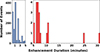 |
Fig. 7. Histogram of the differences between the last and first timestamps of detected enhancements for each pixel. The majority of events last ≤5 minutes, justifying the selection of a 5-minute interpolation window for GPR. Events with durations > 5 minutes (19 cases highlighted in red) are excluded from further analysis. |
Finally, for each observation, we computed the cumulative percentage of test points that fell outside the predicted 3σ, 2σ, and 1σ confidence intervals. Ideally, for well-calibrated models, these percentages should match their theoretical expectations (0.27%, 4.55%, and 31.73%, respectively). This provides a statistical overview of the model’s uncertainty calibration across the entire observation, even though the prediction intervals themselves are computed for individual points. In principle, rigorous evaluation of point-wise prediction intervals would require knowledge of the true underlying function and the use of simulated datasets (Sluijterman et al. 2024). While we ultimately report 3σ uncertainties, evaluating multiple confidence levels provides a more complete picture of the model’s probabilistic calibration. As seen in Fig. 8, at the 3σ level, the Matérn kernel generally performs better than the RBF kernel, with observed outlier rates remaining close to the expected 0.3% threshold, albeit with mild overconfidence. At the 2σ level, the Matérn kernel again shows relatively good agreement with theoretical expectations, while the RBF kernel is slightly overconfident. At the 1σ level, both models show under-confidence, with fewer outliers than expected. Importantly, even in the worst-performing flare class, the Matérn kernel still captures ≈98.5% of test points within the 3σ interval. Thus, we selected the Matérn kernel over the RBF kernel, which gives the final functional form of the kernel as
 (1)
(1)
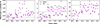 |
Fig. 8. Percentage of test points outside the predicted 3σ (left), 2σ (middle), and 1σ (right) prediction interval, shown for Gaussian process models using Matérn (magenta) and RBF (black) kernels. The horizontal dotted lines represent the theoretical expected percentage of points that lie outside the “n” sigma prediction interval. The RBF kernel overshoots the percentage of points outside the prediction interval compared to Matérn in most flare classes for the 3σ performance evaluation, rendering the Matérn kernel the better choice for uncertainty estimation. |
where r refers to the separation between any two data points and l refers to the characteristic length-scale.
Notably, uncertainty quantification is significantly better calibrated for B-class flares, as indicated by the low percentage of points falling outside the nσ confidence intervals. A plausible explanation for this is that B-class flares typically involve smaller flaring regions, resulting in fewer time series being affected by dynamic, flare-related fluctuations. If poorly modeled segments correlate with heated regions, then smaller flare areas may inherently lead to better GPR fits.
3. Results
3.1. Occurrence statistics of NUV continuum enhancements
Using the detection methods described in Sect. 2.2, we find the following:
-
Intensity threshold results: Of 234 flare candidates (some of which were not ideally observed by the spectrograph slit), the intensity threshold method followed by FUV-based filtering identified NUV continuum enhancements in 26 flares. These included six X-class, six M-class, and 14 C-class events. All detected enhancements were above the 3σ significance level.
-
IF results: Applying the IF method followed by FUV filtering yielded detections in 80 flares, consisting of nine X-class, 22 M-class, 48 C-class, and one B-class events. Among these, 49 flares have at least one pixel with enhancement above the 3σ threshold. The breakdown of the flares with 3σ detections is as follows: seven X-class, 15 M-class, 26 C-class, and one B-class flare. For details of these observations, we refer to Table A.1.
Based on the detection statistics, the IF method detected ≥3σ enhancements in 20.9% of all candidates, compared to 11.1% using the intensity threshold method. The number of 3σ detections is generally higher with the IF algorithm across flare events, and it also succeeds in detecting enhancements associated with weaker flares; see Fig. 9 for a comparison of the detection performance of the two algorithms. It is important to note that a few detected NUV enhancements are associated with events not listed in the GOES flare catalog (e.g., Fig. 10). Consequently, a time series centered around a reported GOES flare may contain an unreported flare and its associated enhancement. In such cases, the enhancement could be mistakenly attributed to the GOES-reported flare, introducing ambiguity in the analysis. To ensure reliable attribution of enhancements, such ambiguous events were excluded from the statistics in Figs. 12, 14, A.2, and A.3. These excluded cases for the IF pipeline include nine C-class and five M-class flares.
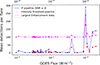 |
Fig. 9. Comparison of detection performances between the IF-based (≥3σ) and intensity threshold-based enhancement detection methods. The y-axis shows the mean number of detected enhancement timestamps per flare, normalized by the number of flares in each GOES flux bin. The GPR-based pipeline consistently identifies more enhancement timestamps across the flare flux range. The magenta curve shows the maximum number of enhanced pixels corresponding to a full raster scan (arbitrary scaling). |
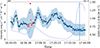 |
Fig. 10. Misattributed NUV continuum enhancement caused by an unrecognized flare (27-10-2014 16:56–17:02), within a time series clipped around a GOES-reported M-class flare (vertical dotted blue line). The red stars represent the 5-minute segment excluded for GPR interpolation; and the magenta circle marks the detected enhancement. The black curve and blue-shaded region represent the GPR mean and 3σ confidence interval. The GOES X-ray flux is shown as the dotted blue curve. |
3.2. Spatial and temporal characteristics of NUV continuum enhancements
Spatial characteristics: No instances of NUV continuum enhancements accompanied by FUV enhancements were found in the quiet Sun. In the flaring regions, all enhanced pixels lie on the flare ribbons. Interestingly, these enhancements were generally observed to occur in a subregion of the flare ribbons, as seen in Fig. 11. On further investigation of a few cases, the enhancements appear mostly at the edges of the flare ribbons. Figure A.1 shows one example demonstrating that even with relaxed significance thresholds, enhancements remain confined to the ribbon edges. Therefore, there may still be cases with no detected enhancements even though a part of the ribbon is observed by the spectrograph’s slit. The magenta curve in Fig. 9 shows the largest count of enhanced pixels from among all the enhanced rasters. The arbitrary scaled values represent the largest spatial extent of enhancement during the flare, enabling comparison of the relative enhanced areas between different observations. It is worth noting that comparisons between the actual number of enhanced pixels cannot be made, as the spatial coverage of the flare by the IRIS slit varies significantly between observations. From our sample of 48 C-class, 22 M-class, and nine X-class flares, flares with a higher mean number of detections also exhibit larger enhancement areas at some point in time, with X-class flares showing the largest enhancement area, followed by M-class (albeit only a single flare), and then C-class flares.
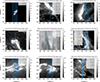 |
Fig. 11. Spatial and temporal information of NUV continuum enhancements detected using the IF pipeline. The horizontal markers show the spatial locations of significant enhancements, with thresholds set at 3σ for the C-class, 5σ for the M- and X-classes, and 14σ for the X2.0 flare to reduce visual clutter in stronger events. Thus, the area of enhancement is not directly comparable. All enhanced pixels lie on the flare ribbons; any apparent spatial offsets arise from plotting multiple enhancement timestamps onto a single SJI frame. Each color represents a specific raster (i.e., all raster steps from a single raster scan), where each raster step corresponds to a different time. |
Temporal characteristics: Most of the enhancements detected by the intensity threshold pipeline show a sharp impulsive rise followed by an exponential-like decay (see Fig. 2). These events are consistently associated with well-defined GOES soft X-ray flares and predominantly occurred up to approximately 25 minutes after the GOES start time and 30 minutes before the GOES peak time (see Fig. 12). In contrast, the IF-based detection pipeline identified enhancements across a broader temporal range (partially because we fed it a longer time series), ranging from 20 minutes before to 70 minutes after the GOES start time, and from 50 minutes before to 40 minutes after the GOES peak time, with most of the enhancements lasting ≤5 min ±2× cadence (see Fig. 7). In a few cases (4 pixels overall) – for example, enhancements occurring approximately 10 and 20 minutes before the GOES start time or > 20 min after the GOES peak time – enhancements were detected without clear corresponding changes in the GOES soft X-ray flux (see Fig. 13), unlike other detected cases (Fig. 6). A visual inspection of such cases showed small-scale brightenings of a maximum of a few pixels in the SJI.
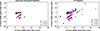 |
Fig. 12. Time offsets of the first detected timestamp of continuum enhancements relative to the GOES soft X-ray flare start time (x-axis) and peak time (y-axis). Each point represents an individual instance (for a specific pixel) of enhancement detection, color-coded by a GOES flare class. Enhancements identified by the intensity threshold pipeline (left) predominantly occur within 0−25 minutes after the GOES start time. In contrast, the IF pipeline (right) provides detections spanning a broader temporal range and detects more enhancements after the impulsive phase of the flares. This is partly because we use an hour-long time series as the input to the IF pipeline in contrast to the 30-minute intensity thresholding time series. The linear patterns observed in the scatter plots arise from the detection of enhancements in temporally consecutive rasters. |
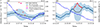 |
Fig. 13. Example time series wherein the IF pipeline detected ≥3σ NUV continuum enhancement with corresponding FUV continuum enhancement but without any apparent change in GOES soft X-ray flux at the timestamps of enhancement. Left: Observation GOES start time (2014-02-11 C-Class flare, raster position 5, pixel 812) at 13:15:00. Right: Observation GOES start time (2015-09-16 B-Class flare, raster position 0, pixel 98) at 13:38:00. NUV continuum enhancements were detected approximately 7 min and 13 min before the GOES start time. |
3.3. Variation of NUV enhancements across flare class
Figure 14 shows the magnitude of ≥3σ NUV continuum enhancements with respect to the corresponding GOES flare flux, identified using the IF detection pipeline. The black points with error bars correspond to measurements at distinct timestamps within enhanced pixel time series, wherein a single pixel may contribute multiple detections. The distribution clearly indicates that X-class flares show both the highest enhancement magnitudes and the largest number of detection instances. Notably, three out of four X-class flares contribute more detections than all M- and C-class flares combined (see Fig. A.2).
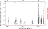 |
Fig. 14. Magnitude of ≥3σ NUV continuum enhancements as a function of GOES flare flux, detected using the IF detection pipeline. The black points with error bars represent the enhancement magnitudes estimated from individual enhanced pixel time series for a specific flare class. A single time series may contain multiple enhanced timestamps and can therefore contribute multiple enhancement magnitude estimates to the plot. A jittered version of this plot, included in the appendix Fig. A.2, shows the density of detections. The total number of flares contributing to these measurements is shown by the red crosses. Stronger enhancements are predominantly observed for the most energetic (X-class) flares. |
While some C-class flares show enhancement magnitudes that approach or exceed those in M-class flares, the associated uncertainties ranging up to 100% in some cases limit the ability to draw statistically significant conclusions. The C-class enhancements show larger relative uncertainties, while M-class flares display enhancements with tighter error bars. A trend of increasing enhancement magnitude with flare class is evident in the detections made using the intensity threshold pipeline (see Fig. A.3). Some flares show notably fewer and weaker detections, likely because the IRIS slit did not sufficiently cover the flare ribbons. Enhancement detections in the lower flare classes are more uncertain, likely due to their intrinsic flare weakness and low signal-to-noise ratio. Only a single pixel corresponding to a B-class event satisfied the detection criteria and was therefore excluded from a statistical interpretation. The concentration of detections at higher flux levels may be attributed to the larger enhancement areas of stronger flares (see Fig. 9).
4. Discussion
4.1. Location of NUV enhancements on flare ribbons
Spatial analysis of continuum enhanced pixels in events such as those shown in Fig. 11 reveals that continuum enhancements are confined to localized regions of the flare ribbon, specifically the ribbon edges; see Fig. A.1. In the WLF detection regime, enhancements are reported to be concentrated near the central regions of flare kernels, which are attributed to preferred energy deposition in the central regions (Song et al. 2018). This difference in the location of NUV enhancements and visible continuum enhancements might be attributed to the lower spatial resolution of HMI or to the use of pseudo-continuum intensity estimates (Švanda et al. 2018). However, the location need not be the same if the physical mechanism of the enhancement differs for the two wavelength regimes. Because flare ribbon fronts mark the chromospheric footpoints of newly reconnected field lines and our detections lie near ribbon edges, this raises the possibility that the enhancements are co-spatial with the ribbon-front locations exhibiting the peculiar Mg II line profiles (Panos et al. 2018), He I 10830 Å dimming (Xu et al. 2016), and Ca II and He I profiles showing transitions between up-flows and down-flows on timescales of order 10 s (Kuckein et al. 2025). In terms of flare energetics, this would mean that the enhancements occur predominantly in the regions with freshly reconnected magnetic field lines. Recent simulations of Mg II emission at ribbon fronts suggest that the high-energy flux injected during their lifetime is relatively modest and more gradual than that in regular bright ribbon regions. These ribbon-front areas exhibit weaker chromospheric evaporation than the bright ribbon regions (Polito et al. 2023). Indeed, a visual inspection of a few spectra from locations with enhancements shows peculiar Mg II spectra similar to the ribbon-front categories found by Panos et al. (2018), though we also find other types of flare spectra whose analysis will be conducted in future work. Such a study would help us understand whether regions with relatively modest high-energy particle flux and gradual injection (simulated as a triangular electron-beam injection profile that peaks at 10 s, rather than a constant flux profile; see Polito et al. 2023) are the preferred sites for NUV continuum enhancements.
4.2. Comparison of NUV and WL continuum emission
Our results demonstrate clear differences in the performances of the two detection pipelines. The IF pipeline achieved more detections than the intensity threshold method, suggesting that a significant number of genuine NUV continuum enhancements are missed by thresholding applied to the IRIS data. However, the overall detection rate remains lower than that reported for WLF studies (Castellanos Durán & Kleint 2020; Cai et al. 2024), wherein the detections reach a rate of > 50% of the events. One reason for this discrepancy may be that visible detections were performed using pseudo-continuum intensity estimates (Švanda et al. 2018) from an imaging instrument (HMI), whereas our NUV detections rely on a slit spectrograph, where capturing the time and location of the enhancement is more difficult. This reasoning is supported by our results showing that these enhancements are predominantly concentrated in the flare ribbon edges; hence, it is important not only to capture the flare ribbon but also to observe the specific subregion of the ribbon where the continuum enhancement occurs.
In terms of temporal evolution, we observe that NUV continuum enhancements occur primarily during the impulsive phase of the flares, but in some strong flares, they also occur up to 20 min after the GOES peak time. Traditionally, enhancements aligned temporally with the impulsive phase have been interpreted as signatures of nonthermal electron-beam heating and associated hydrogen recombination in the chromosphere. Jing et al. (2024), however, reported a M4.5 and a M1.6 WLF whose white-light emission peaks occurred ≈10 min after the soft X-ray maximum. These enhancements were hypothesized to be associated with the cooling phase of the flare. Our results also suggest that enhancements are not limited solely to the impulsive phase. We speculate the possibility of multiple episodes of energy deposition, potentially involving repeated electron-beam bombardment (Nishizuka et al. 2010).
Moreover, a few single-pixel NUV continuum enhancements (three to four cases) do not correlate with soft X-ray profile changes, leading us to speculate that they correspond to the decay-phase from earlier flares or small reconnection events in the solar atmosphere. In reference to Fig. 13, no GOES-reported flare precedes the C-class flare, while a C-class event immediately precedes the B-class flare. These detections correspond to small, spatially localized bright points structurally indistinct from other features in their vicinity. They appear identical to flare-related NUV enhancements in the NUV and FUV continua but occur very rarely (four cases in the 250 analyzed flares) and are limited to single-pixel detections on the IRIS slit.
4.3. Spatial correspondence between NUV and FUV enhancements
We find spatial and temporal correlations between NUV and FUV continuum enhancements during flares. We discovered that strong NUV continuum enhancements were accompanied by FUV continuum enhancements; however, this does not rule out the possibility of the two occurring independently. Radiative hydrodynamic simulations of strong flares have shown that the recombination of free electrons with protons, following hydrogen ionization by nonthermal electron beams, can account for the NUV continuum emission (Heinzel et al. 2016; Kowalski et al. 2017). In contrast, the FUV continuum near 1520 Å and 1680 Å is believed to arise from the recombination continua of neutral silicon. These continua are believed to be produced when neutral silicon atoms near the temperature-minimum region of the lower chromosphere are photoionized by intense flare UV line emission originating from the upper chromosphere and transition region (e.g., C II and C IV). The subsequent recombination of electrons with Si II ions emits the observed FUV continuum (Doyle & Phillips 1992). Flare simulations have not yet compared the formation mechanisms of the FUV and NUV continua. We plan to investigate this in future work using hydrodynamic simulations of the flare candidates in our study.
5. Conclusions
In this study, we developed and applied two continuum enhancement detection pipelines to IRIS spectral data. For one pipeline, we used a machine learning algorithm to obtain the uncertainties over enhancements, which allowed us to detect enhancements within the granulation levels in flares as weak as C1.1 class. Below we list our main findings:
-
Based on the analysis of 243 flare cases, 3σ significant NUV continuum enhancements were detected using the IF detection pipeline in 49 flares, which is twice the number of detections obtained using the intensity threshold approach. This number appears relatively low compared to continuum enhancements detected in imaging data in the WLF regime, primarily because IRIS is a slit spectrograph.
-
The NUV continuum enhancements occur predominantly on the flare ribbon edges. This suggests the possibility that the enhancements occur in regions with freshly reconnected magnetic field lines or the ribbon fronts. There have been previous findings of peculiar Mg II line profiles, short-lived upflows, and He I dimming at the ribbon fronts during flares. Whether NUV continuum enhancement preferably occurs at the location of the above-mentioned features remains to be verified in future work.
-
The detected enhancements are stronger for more energetic flares and occur predominantly in the impulsive phase of the flare but also up to 20 min after the GOES peak time for strong flares. This suggests the possibility of multiple reconnection events. Moreover, in four cases, single-pixel enhancement detections did not correspond with any clear change in GOES soft X-ray flux. These enhancements were located on morphologically indistinct bright points in the active regions, which could signify small-scale energy deposition events.
-
Finally, NUV and FUV enhancements correspond spatially and temporally. This finding allowed us to distinguish NUV continuum enhancements from other variations in the continuum time series. Future studies planning to simulate either of the continua could use this spatial and temporal correspondence to constrain models. Understanding the physical origin of this correspondence is planned for future work.
The enhancement strength derived in this study will help us constrain the flare simulation models not only for strong flare events, as done in previous studies, but also for different flare energies. The beam parameters in the flare simulations govern the penetration depth of the electrons into the solar atmosphere (Carlsson et al. 2023). A clear extension of this work is to understand the relation between the flare beam parameters obtained from HXR data and the NUV continuum enhancement observables from this study. While previous studies have focused more on strong X-class events, we aim to understand whether the same underlying process for strong flares can also explain the observed enhancement in weak flares.
Acknowledgments
This work was supported by a SNSF PRIMA grant and a SERI-funded ERC CoG grant. We are grateful to LMSAL for allowing us to download the IRIS database. IRIS is a NASA small explorer mission developed and operated by LMSAL with mission operations executed at NASA Ames Research Center and major contributions to downlink communications funded by ESA and the Norwegian Space Centre. This research has used NASA’s Astrophysics Data System Bibliographic Services. Some of our calculations were performed on UBELIX (http://www.id.unibe.ch/hpc), the HPC cluster at the University of Bern. We thank the referee for his/her valuable comments and suggestions. We are grateful to our colleagues from the space weather group at the University of Bern: Dr. Michelle Galloway, Vanessa Mercea, Moritz Meyer zu Westram and Dorian Paillon for helpful discussions that contributed in shaping the methodology of this study. The authors also thank Dr. Phil Judge for helpful discussions on the interpretation of this work.
References
- Allred, J. C., Hawley, S. L., Abbett, W. P., & Carlsson, M. 2005, ApJ, 630, 573 [NASA ADS] [CrossRef] [Google Scholar]
- Cai, Y., Hou, Y., Li, T., & Liu, J. 2024, ApJ, 975, 69 [Google Scholar]
- Carlsson, M., Fletcher, L., Allred, J., et al. 2023, A&A, 673, A150 [NASA ADS] [CrossRef] [EDP Sciences] [Google Scholar]
- Castellanos Durán, J. S., & Kleint, L. 2020, ApJ, 904, 96 [CrossRef] [Google Scholar]
- De Pontieu, B., Title, A. M., Lemen, J. R., et al. 2014, Sol. Phys., 289, 2733 [Google Scholar]
- Doyle, J. G., & Phillips, K. J. H. 1992, A&A, 257, 773 [Google Scholar]
- Heinzel, P., & Kleint, L. 2014, ApJ, 794, L23 [NASA ADS] [CrossRef] [Google Scholar]
- Heinzel, P., Kašparová, J., Varady, M., Karlický, M., & Moravec, Z. 2016, IAU Symp., 320, 233 [NASA ADS] [Google Scholar]
- Hirzberger, J., Bonet, J. A., Vázquez, M., & Hanslmeier, A. 1999, ApJ, 515, 441 [NASA ADS] [CrossRef] [Google Scholar]
- Hudson, H. S. 1972, Sol. Phys., 24, 414 [Google Scholar]
- Jess, D. B., Mathioudakis, M., Crockett, P. J., & Keenan, F. P. 2008, ApJ, 688, L119 [NASA ADS] [CrossRef] [Google Scholar]
- Jing, Z., Li, Y., Feng, L., et al. 2024, Sol. Phys., 299, 11 [Google Scholar]
- Joshi, R., Schmieder, B., Heinzel, P., et al. 2021, A&A, 654, A31 [NASA ADS] [CrossRef] [EDP Sciences] [Google Scholar]
- Kleint, L., Heinzel, P., Judge, P., & Krucker, S. 2016, ApJ, 816, 88 [CrossRef] [Google Scholar]
- Kleint, L., Heinzel, P., & Krucker, S. 2017, ApJ, 837, 160 [NASA ADS] [CrossRef] [Google Scholar]
- Kowalski, A. F., Allred, J. C., Daw, A., Cauzzi, G., & Carlsson, M. 2017, ApJ, 836, 12 [NASA ADS] [CrossRef] [Google Scholar]
- Kretzschmar, M. 2011, A&A, 530, A84 [NASA ADS] [CrossRef] [EDP Sciences] [Google Scholar]
- Kuckein, C., Collados, M., Asensio Ramos, A., et al. 2025, A&A, 699, A121 [NASA ADS] [CrossRef] [EDP Sciences] [Google Scholar]
- Liu, F. T., Ting, K. M., & Zhou, Z.-H. 2012, ACM Trans. Knowl. Discov. Data, 6, 1 [Google Scholar]
- Machado, M. E., Emslie, A. G., & Avrett, E. H. 1989, Sol. Phys., 124, 303 [NASA ADS] [CrossRef] [Google Scholar]
- Milligan, R. O., & McElroy, S. A. 2013, ApJ, 777, 12 [Google Scholar]
- Najita, K., & Orrall, F. Q. 1970, Sol. Phys., 15, 176 [NASA ADS] [CrossRef] [Google Scholar]
- Neidig, D. F. 1989, Sol. Phys., 121, 261 [NASA ADS] [CrossRef] [Google Scholar]
- Nishizuka, N., Takasaki, H., Asai, A., & Shibata, K. 2010, ApJ, 711, 1062 [NASA ADS] [CrossRef] [Google Scholar]
- Panos, B., Kleint, L., Huwyler, C., et al. 2018, ApJ, 861, 62 [Google Scholar]
- Polito, V., Kerr, G. S., Xu, Y., Sadykov, V. M., & Lorincik, J. 2023, ApJ, 944, 104 [NASA ADS] [CrossRef] [Google Scholar]
- Rasmussen, C. E. 2004, Lect. Notes Comput. Sci., 3176 [Google Scholar]
- Sluijterman, L., Cator, E., & Heskes, T. 2024, Neural Networks, 173, 106203 [Google Scholar]
- Song, Y. L., Tian, H., Zhang, M., & Ding, M. D. 2018, A&A, 613, A69 [NASA ADS] [CrossRef] [EDP Sciences] [Google Scholar]
- Švanda, M., Jurčák, J., Kašparová, J., & Kleint, L. 2018, ApJ, 860, 144 [CrossRef] [Google Scholar]
- Xu, Y., Cao, W., Ding, M., et al. 2016, ApJ, 819, 89 [Google Scholar]
- Xu, Z., Yan, X., Li, Z., et al. 2025, ApJ, 986, L15 [Google Scholar]
- Zbinden, J., Kleint, L., & Panos, B. 2024, A&A, 689, A72 [NASA ADS] [CrossRef] [EDP Sciences] [Google Scholar]
- Zuccarello, F., Guglielmino, S. L., Capparelli, V., et al. 2020, ApJ, 889, 65 [NASA ADS] [CrossRef] [Google Scholar]
Appendix A: Additional figures
A.1. Enhancement at the ribbon edges
To avoid clutter while still conveying the spatial distribution of NUV continuum enhancements, stringent sigma thresholds were applied in Fig. 11. However, to more clearly illustrate that these enhancements occur on the edges of the flare ribbon, it is necessary to show all detected enhancements regardless of their significance and not have them overlaid on a single SJI frame. Figure A.1 provides such an example. For the SJI timestamp 16:23:17, the first instances of continuum enhancement are marked in magenta and occurred between 16:23:13 and 16:24:28. Although there is a cadence mismatch between the SJI images and the raster steps–raising the possibility that the ribbon was larger before 16:23:17 and the enhancements initially spanned the entire ribbon. The progression of the flare ribbon was examined to address this ambiguity. We find that the ribbon continued to grow in size until 16:25:28, and that it had approximately the same spatial extent between 16:22:58 and 16:23:17. Therefore, we conclude that the detected enhancements at that time were confined to the edge of the flare ribbon.
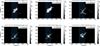 |
Fig. A.1. Spatial and temporal characteristics of NUV continuum enhancements detected using the IF pipeline. Horizontal markers show the spatial locations of NUV enhancements, without applying any significance threshold. Although there is a time difference between the SJI image timestamp and the earliest NUV enhancement detection (plotted in magenta), the flare ribbon remains relatively unchanged in size between 16:22:58 and 16:23:17. Therefore, the magenta enhancement lies on the edge of the flare ribbon. After 16:25:28 the ribbon begins to shrink in size. |
Summary of IRIS flares with detected near-ultraviolet (NUV) enhancements above the 3σ level using IF pipeline. The enhancement time indicates the duration over which enhancements were detected; however, enhancements may not persist throughout the entire interval. In some cases, no corresponding flare was reported by GOES during the listed enhancement interval, which may result in misattribution.
A.2. Magnitude of enhancement: Detections from both pipelines
Figure 14 presents the variation in the magnitude of NUV continuum enhancements across flare classes but it lacks the resolution to reveal trends within individual classes (e.g., across all M-class flares) and does not convey the density of detections. To address this, Figure A.2 includes small random offsets (jitter) applied to the flare flux values to reduce over-plotting and improve visualization. The jitter is introduced by multiplying the original flare flux by 100.06. This perturbation is small enough to preserve the broad separation between C-, M-, and X-class flares, though slight overlap between adjacent class boundaries (e.g., M9.9 and X1.0) may occur. Consequently, this figure should not be used to infer trends across flare classes; Figure 14 remains the more appropriate figure for such comparisons. The figure shows that there are a significantly greater number of detections associated with X-class flares, compared to M-, C-, and B-class flares.
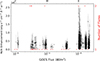 |
Fig. A.2. Magnitude of ≥3σ NUV continuum enhancements across different GOES flare flux, detected using the IF pipeline. Small random offsets (jitter) have been applied to the flare flux axis to reduce overlap and improve visualization. The marker definitions are consistent with those used in Fig. 14. The introduction of jitter helps show a clear trend of increasing enhancement magnitude within the M-class flare regime. However, a few detections from X1.0-class flares may overlap with the M9.9-class region due to the jitter, which is why Figure 14 should be consulted in parallel for accurate interpretation. |
Figure A.3 shows the enhancements detected using the intensity threshold pipeline, which results in fewer overall detections, but with narrower uncertainty intervals. Apart from a single C-class flare with a large uncertainty, the trend of increasing enhancement magnitude with increasing flare strength appears clearer in the results using this pipeline.
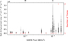 |
Fig. A.3. Magnitude of ≥3σ NUV continuum enhancements as a function of GOES flare flux, detected using the intensity threshold detection pipeline, plotted without jitter. Marker definitions are consistent with those in Fig. 14. With the exception of one C-class flare showing a wide prediction interval, the enhancement magnitude generally increases with flare class. A few flares show significantly fewer and weaker detections, which is likely due to limited coverage of the flare ribbons by the IRIS slit. |
All Tables
Summary of IRIS flares with detected near-ultraviolet (NUV) enhancements above the 3σ level using IF pipeline. The enhancement time indicates the duration over which enhancements were detected; however, enhancements may not persist throughout the entire interval. In some cases, no corresponding flare was reported by GOES during the listed enhancement interval, which may result in misattribution.
All Figures
|
Fig. 1. Observed Mg II h and k spectrum, with the continuum windows used in this study (vertical dashed lines). The continuum windows are located far from the wings of the strong resonant Mg II lines at 2796 and 2803 Å. Bottom: Magnified views of the selected continuum regions. The blue spectrum corresponds to the time when the continuum emission was enhanced, while the orange spectrum represents the post-enhancement period during the flare’s impulsive phase. |
| In the text | |
|
Fig. 2. Impulsive increase observed in the NUV continuum (2826 Å window; solid line), the peak intensity of the Mg II k line (dashed line), and the FUV continuum emission proxy (dotted line) at pixel (pxl) 316 (blue), raster position (rr) 3, during an X-class flare on 27-10-2014 at 14:23:12. In contrast, no such behavior is seen in the time series of other pixels on the same raster position, such as pixel 200 (pink line). Refer to Fig. 3 for the SJI image. |
| In the text | |
|
Fig. 3. Slit-jaw image in the 2832 Å continuum window of an active region during a solar flare, showing enhanced NUV continuum emission near the center right. The SJI observation time was 27-10-2014 at 14:23:16.950. |
| In the text | |
|
Fig. 4. Flowchart of the methodology used in this study, highlighting the differences in outlier detection and uncertainty estimation between the intensity threshold and IF approaches. The letter ‘c’ refers to the contamination parameter, which controls the proportion of detected outliers. GPR is used for uncertainty estimation (see Sect. 2.2.3 for details). |
| In the text | |
|
Fig. 5. Example of continuum emission in FUV, corresponding to the timestamp of enhanced continuum emission seen in NUV (refer to Fig. 2). Right: Example timestamp, with no continuum emission above our threshold. The vertical brown markers along the x-axis indicate the 50 equally spaced wavelength points used in defining the FUV bright-band detection criterion. |
| In the text | |
|
Fig. 6. Comparison between outlier detections, using the three-sigma threshold (blue-shaded region) around the mean (horizontal solid black line) and IF with a contamination parameter of 0.1. The colored points are outlier candidates detected by IF, and the red points are true positive enhancements filtered by detecting corresponding FUV continuum emission. Top: 2014-10-22 M-class flare with the IF accurately detecting the rising and decay phase of the enhancement. Bottom: 2014-03-29 X-class flare, with the IF detecting enhancements in cases where a simple intensity threshold would fail. The dotted blue curve represents the GOES flux. The dotted magenta curve represents the time derivative of the 3 s averaged GOES flux (arbitrarily scaled), often used as a proxy signature of nonthermal processes. |
| In the text | |
|
Fig. 7. Histogram of the differences between the last and first timestamps of detected enhancements for each pixel. The majority of events last ≤5 minutes, justifying the selection of a 5-minute interpolation window for GPR. Events with durations > 5 minutes (19 cases highlighted in red) are excluded from further analysis. |
| In the text | |
|
Fig. 8. Percentage of test points outside the predicted 3σ (left), 2σ (middle), and 1σ (right) prediction interval, shown for Gaussian process models using Matérn (magenta) and RBF (black) kernels. The horizontal dotted lines represent the theoretical expected percentage of points that lie outside the “n” sigma prediction interval. The RBF kernel overshoots the percentage of points outside the prediction interval compared to Matérn in most flare classes for the 3σ performance evaluation, rendering the Matérn kernel the better choice for uncertainty estimation. |
| In the text | |
|
Fig. 9. Comparison of detection performances between the IF-based (≥3σ) and intensity threshold-based enhancement detection methods. The y-axis shows the mean number of detected enhancement timestamps per flare, normalized by the number of flares in each GOES flux bin. The GPR-based pipeline consistently identifies more enhancement timestamps across the flare flux range. The magenta curve shows the maximum number of enhanced pixels corresponding to a full raster scan (arbitrary scaling). |
| In the text | |
|
Fig. 10. Misattributed NUV continuum enhancement caused by an unrecognized flare (27-10-2014 16:56–17:02), within a time series clipped around a GOES-reported M-class flare (vertical dotted blue line). The red stars represent the 5-minute segment excluded for GPR interpolation; and the magenta circle marks the detected enhancement. The black curve and blue-shaded region represent the GPR mean and 3σ confidence interval. The GOES X-ray flux is shown as the dotted blue curve. |
| In the text | |
|
Fig. 11. Spatial and temporal information of NUV continuum enhancements detected using the IF pipeline. The horizontal markers show the spatial locations of significant enhancements, with thresholds set at 3σ for the C-class, 5σ for the M- and X-classes, and 14σ for the X2.0 flare to reduce visual clutter in stronger events. Thus, the area of enhancement is not directly comparable. All enhanced pixels lie on the flare ribbons; any apparent spatial offsets arise from plotting multiple enhancement timestamps onto a single SJI frame. Each color represents a specific raster (i.e., all raster steps from a single raster scan), where each raster step corresponds to a different time. |
| In the text | |
|
Fig. 12. Time offsets of the first detected timestamp of continuum enhancements relative to the GOES soft X-ray flare start time (x-axis) and peak time (y-axis). Each point represents an individual instance (for a specific pixel) of enhancement detection, color-coded by a GOES flare class. Enhancements identified by the intensity threshold pipeline (left) predominantly occur within 0−25 minutes after the GOES start time. In contrast, the IF pipeline (right) provides detections spanning a broader temporal range and detects more enhancements after the impulsive phase of the flares. This is partly because we use an hour-long time series as the input to the IF pipeline in contrast to the 30-minute intensity thresholding time series. The linear patterns observed in the scatter plots arise from the detection of enhancements in temporally consecutive rasters. |
| In the text | |
|
Fig. 13. Example time series wherein the IF pipeline detected ≥3σ NUV continuum enhancement with corresponding FUV continuum enhancement but without any apparent change in GOES soft X-ray flux at the timestamps of enhancement. Left: Observation GOES start time (2014-02-11 C-Class flare, raster position 5, pixel 812) at 13:15:00. Right: Observation GOES start time (2015-09-16 B-Class flare, raster position 0, pixel 98) at 13:38:00. NUV continuum enhancements were detected approximately 7 min and 13 min before the GOES start time. |
| In the text | |
|
Fig. 14. Magnitude of ≥3σ NUV continuum enhancements as a function of GOES flare flux, detected using the IF detection pipeline. The black points with error bars represent the enhancement magnitudes estimated from individual enhanced pixel time series for a specific flare class. A single time series may contain multiple enhanced timestamps and can therefore contribute multiple enhancement magnitude estimates to the plot. A jittered version of this plot, included in the appendix Fig. A.2, shows the density of detections. The total number of flares contributing to these measurements is shown by the red crosses. Stronger enhancements are predominantly observed for the most energetic (X-class) flares. |
| In the text | |
|
Fig. A.1. Spatial and temporal characteristics of NUV continuum enhancements detected using the IF pipeline. Horizontal markers show the spatial locations of NUV enhancements, without applying any significance threshold. Although there is a time difference between the SJI image timestamp and the earliest NUV enhancement detection (plotted in magenta), the flare ribbon remains relatively unchanged in size between 16:22:58 and 16:23:17. Therefore, the magenta enhancement lies on the edge of the flare ribbon. After 16:25:28 the ribbon begins to shrink in size. |
| In the text | |
|
Fig. A.2. Magnitude of ≥3σ NUV continuum enhancements across different GOES flare flux, detected using the IF pipeline. Small random offsets (jitter) have been applied to the flare flux axis to reduce overlap and improve visualization. The marker definitions are consistent with those used in Fig. 14. The introduction of jitter helps show a clear trend of increasing enhancement magnitude within the M-class flare regime. However, a few detections from X1.0-class flares may overlap with the M9.9-class region due to the jitter, which is why Figure 14 should be consulted in parallel for accurate interpretation. |
| In the text | |
|
Fig. A.3. Magnitude of ≥3σ NUV continuum enhancements as a function of GOES flare flux, detected using the intensity threshold detection pipeline, plotted without jitter. Marker definitions are consistent with those in Fig. 14. With the exception of one C-class flare showing a wide prediction interval, the enhancement magnitude generally increases with flare class. A few flares show significantly fewer and weaker detections, which is likely due to limited coverage of the flare ribbons by the IRIS slit. |
| In the text | |
Current usage metrics show cumulative count of Article Views (full-text article views including HTML views, PDF and ePub downloads, according to the available data) and Abstracts Views on Vision4Press platform.
Data correspond to usage on the plateform after 2015. The current usage metrics is available 48-96 hours after online publication and is updated daily on week days.
Initial download of the metrics may take a while.