| Issue |
A&A
Volume 701, September 2025
|
|
|---|---|---|
| Article Number | A88 | |
| Number of page(s) | 21 | |
| Section | Galactic structure, stellar clusters and populations | |
| DOI | https://doi.org/10.1051/0004-6361/202554020 | |
| Published online | 04 September 2025 | |
Bar-spiral interaction induces radial migration and star formation bursts
1
Leibniz-Institüt für Astrophysik Potsdam (AIP), An der Sternwarte 16, 14482 Potsdam, Germany
2
Universität Potsdam, Institut für Physik und Astronomie, Karl-Liebknecht-Str. 24–25, 14476 Potsdam, Germany
3
MAUCA – Master track in Astrophysics, Université Côte d’Azur, Observatoire de la Côte d’Azur, Parc Valrose, 06100 Nice, France
4
NSF Astronomy & Astrophysics Postdoctoral Fellow, Department of Astronomy, University of Wisconsin–Madison, Madison, WI 53706, USA
5
Universität Heidelberg, Interdisziplinäres Zentrum für Wissenschaftliches Rechnen, Im Neuenheimer Feld 205, 69120 Heidelberg, Germany
6
Universität Heidelberg, Zentrum für Astronomie, Institut für Theoretische Astrophysik, Albert-Ueberle-Straße 2, 69120 Heidelberg, Germany
7
Astrophysics Research Institute, Liverpool John Moores University, 146 Brownlow Hill, Liverpool L3 5RF, UK
8
Université Côte d’Azur, Observatoire de la Côte d’Azur, CNRS, Laboratoire Lagrange, 06000 Nice, France
9
School of Mathematical and Physical Sciences, Macquarie University, Sydney, NSW 2109, Australia
10
Macquarie University Research Centre for Astrophysics and Space Technologies, Sydney, NSW 2109, Australia
★ Corresponding authors: This email address is being protected from spambots. You need JavaScript enabled to view it.
; This email address is being protected from spambots. You need JavaScript enabled to view it.
Received:
4
February
2025
Accepted:
20
June
2025
Abstract
Context. Central bars and spirals are known to impact significantly the evolution of their host galaxies, both in terms of dynamics and star formation. Their typically different pattern speeds cause them to regularly overlap, which induces fluctuations in bar parameters.
Aims. In this paper, we analyze both numerical simulations of disk galaxies and observational data to study the effect of bar-spiral physical overlap on stellar radial migration and star formation in the bar vicinity, as a function of time and galactic azimuth.
Methods. We studied three different numerical models, two of which are in a cosmological context, alongside APOGEE DR17 data and the WISE catalog of Galactic HII regions.
Results. We find that periodic boosts in stellar radial migration occur when the bar and spiral structures overlap. This mechanism causes net inward migration along the bar leading side, while stars along the bar trailing side and minor axis are shifted outward. The signature of bar-spiral-induced migration is seen between the bar inner Lindbald resonance and well outside its corotation, beyond which other drivers take over. We also find that, in agreement with simulations, APOGEE DR17 stars born at the bar vicinity (which are mostly metal rich) can migrate out to the solar radius while remaining on cold orbits. For the Milky Way, 13% of stars in the solar vicinity with an eccentricity <0.5 were born inside the bar, compared to 5–20% in the simulations. Bar-spiral reconnections also result in periodic starbursts at the bar ends with an enhancement of up to a factor of 4, depending on the strength of the spiral structure. Similarly to the migration bursts, these do not always happen simultaneously at the two sides of the bar, which hints at the importance of odd spiral modes. Data from the WISE catalog suggest this phenomenon is also relevant in our own Galaxy.
Key words: Galaxy: disk / Galaxy: evolution / Galaxy: kinematics and dynamics / solar neighborhood / Galaxy: structure
© The Authors 2025
 Open Access article, published by EDP Sciences, under the terms of the Creative Commons Attribution License (https://creativecommons.org/licenses/by/4.0), which permits unrestricted use, distribution, and reproduction in any medium, provided the original work is properly cited.
This article is published in open access under the Subscribe to Open model. This email address is being protected from spambots. You need JavaScript enabled to view it. to support open access publication.
1 Introduction
Spiral structures are over-dense spiral-shaped regions that emerge from the center of many disk galaxies. Their nature is still debated, between long-lived density waves with a constant rigid-body pattern speed (Lin & Shu 1964; Kalnajs 1973; Bertin & Lin 1996), the overlap of multiple spiral modes (Tagger et al. 1987; Sygnet et al. 1988; Quillen et al. 2011; Minchev et al. 2012), transient material arms that would have the same rotation curve as the stars and gas (Grand et al. 2012a,b; Baba et al. 2013) (although strong bars could increase the spirals’ rotation speed, see, e.g., Grand et al. 2012b; Roca-Fàbrega et al. 2013), or temporary responses to mass clumps in the disk (Toomre & Kalnajs 1991; D’Onghia et al. 2013). Whatever their nature, spirals are very frequent in our local Universe, and 60–70% of spiral galaxies, including the Milky Way (MW), also host a bar feature in their center (Eskridge et al. 2000; Menéndez-Delmestre et al. 2007; Marinova & Jogee 2007; Sheth et al. 2008; Erwin 2018; and Peters 1975; Binney et al. 1991; Blitz & Spergel 1991; Nakada et al. 1991; Weiland et al. 1994; Stanek et al. 1997 for the MW). Both the bar and the spiral structure have essential roles in the evolution of their galaxy; two relevant phenomena studied in this paper are radial migration and star formation.
Radial migration is the change in stellar orbital angular momentum, and thus in guiding radius, and has been seen to occur in numerous N-body simulations of isolated galactic disks (Sellwood & Binney 2002; Roškar et al. 2008; Minchev & Famaey 2010; Grand et al. 2012b), as well as in galaxies simulated in the cosmological context (Minchev et al. 2013; Vincenzo & Kobayashi 2020; Agertz et al. 2021; Lu et al. 2024; Okalidis et al. 2022; Boecker et al. 2023). Several mechanisms can explain migration. Transient spiral structures can cause large-scale migration near their corotation radius as was shown by Sellwood & Binney (2002), Grand et al. (2012b) and Kawata et al. (2014).The transient property here is key, because a long-lived spiral would make the star’s angular momentum go back to its initial value each time the star meets a spiral arm again, instead of truly redistributing stellar angular momenta. The bar, being a more stable pattern, produces migration using different mechanisms. Minchev & Quillen (2006) and Minchev et al. (2011) showed that the overlap of resonances of multiple patterns (such as multiple spiral modes or bar and spiral, respectively) could induce efficient migration in the disk, without requiring a transient spiral structure. This mechanism can also significantly heat stars kinematically and explain the age-velocity dispersion relation in the MW. A bar slowing down rapidly during and right after its formation can also sweep out kinematically cold stars trapped in its resonances, without kinematically heating them, as shown by Khoperskov et al. (2020) (see also Chiba et al. 2021; Chiba & Schönrich 2021; Baba et al. 2024; Zhang et al. 2025). Apart from these secular processes, mergers can similarly provoke radial mixing by introducing an abrupt change in potential (e.g., Quillen et al. 2009; Bird et al. 2012). By moving stars away from their birth place, this process can explain the scatter in the age-metallicity relation in the solar vicinity (e.g., Roškar et al. 2008; Schönrich & Binney 2009) by flattening the radial metallicity gradient at the same time (Minchev et al. 2013). Indeed, in simulations radial migration has been seen to happen mostly outward (e.g., Khoperskov et al. 2021; Agertz et al. 2021; Vincenzo & Kobayashi 2020; Renaud et al. 2025) (although this is likely due to the stellar density decreasing outward) so that metal-rich stars reaching the solar neighborhood (SNd) from the inner disk would increase the local mean metallicity, thus flattening its radial gradient at larger radii. Since migrators that reach the SNd are mostly indistinguishable from locally born stars in their orbital properties; chemical abundances and age information are needed to identify their birth locations, using the technique of chemical tagging (Freeman & Bland-Hawthorn 2002). This is how the first observational evidence for radial migration was suggested by Grenon (1972), Chiappini (2009), and Boeche et al. (2013), and later explicitly found by Kordopatis et al. (2015) using the fact that the local star formation history cannot explain the metallicity of the super-metal-rich ([Fe/H] > 0.25 dex) stars observed in the SNd (Chiappini et al. 2003; Spitoni et al. 2019). In parallel, it is essential to understand how much radial migration must have occurred given the presence of a bar and spiral arms in the MW. Recently, a method to derive birth radii with virtually no dependence on any assumptions on the chemical evolution of the MW was developed by Minchev et al. (2018), Lu et al. (2024), and Ratcliffe et al. (2025), and already used by Ratcliffe et al. (2023, 2025) on APOGEE DR17 red giants to study the evolution of metallicity gradients. This has huge potential to help us quantify the radial dependence of migration in the MW. However, for now only simulations can give us the time evolution of migration.
The relation between bars or spirals and star formation (SF) is also widely researched, and conclusions are still debated. SF is triggered inside molecular clouds when the equilibrium between pressure and gravity is broken in favor of gravity. Overdense regions like spiral arms are thus natural locations for SF to take place. Young stars and molecular clouds are indeed predominantly found in spiral arms (Levine et al. 2006; Poggio et al. 2021; Castro-Ginard et al. 2021; Gaia Collaboration 2023). The chemical signature of spiral arms also shows higher metal-licity in the spiral arms compared to inter-arm regions (Poggio et al. 2022; Hackshaw et al. 2024; Barbillon et al. 2025). However, it is unclear whether spiral arms act as gatherers or triggers of SF. The way to distinguish between these two possibilities is by comparing star formation efficiencies (SFE) between arm and inter-arm regions. Observations are still inconsistent and contradictory. In theory, the gas is shocked when it enters the dense spiral arms, which should trigger SF, as predicted by density wave theory. Several authors found evidence that SFE indeed seemed higher in the spiral arms, which thus supports the triggering scenario (Lord 1987; Vogel et al. 1988; Cepa & Beckman 1990; Lord & Young 1990; Knapen et al. 1996; Seigar & James 2002; Cedrés et al. 2013; Karapetyan et al. 2018). However, other authors found that SFE was generally similar in spiral arms and inter-arm regions, despite local fluctuations (Elmegreen & Elmegreen 1986; Foyle et al. 2010; Moore et al. 2012; Rebolledo et al. 2012; Eden et al. 2015; Ragan et al. 2018; Querejeta et al. 2021, 2024; Sun et al. 2024). The way in which the bar influences SF varies with the bar parameters (Géron et al. 2021, 2023, 2024), and largely depends on temporal and spatial scales. Barred galaxies are believed to funnel gas to the central regions (Combes 1988, 1994; Sakamoto et al. 1999; Carles et al. 2016) thus fueling the higher star formation rates (SFR) there (Sakamoto et al. 1999; Alonso-Herrero & Knapen 2001; Ellison et al. 2011; Coelho & Gadotti 2011; Lin et al. 2020). However, SF is often quenched along the bar (Reynaud & Downes 1998; Sakamoto et al. 1999; Zurita et al. 2004; Khoperskov et al. 2018; Díaz-García et al. 2020; Fraser-McKelvie et al. 2020), and enhanced again at the bar ends (Reynaud & Downes 1998; Sakamoto et al. 1999; Watanabe et al. 2011; Díaz-García et al. 2020; Fraser-McKelvie et al. 2020; Maeda et al. 2020; Géron et al. 2024), right at the interface with spiral arms.
Using two different cosmological simulations, Hilmi et al. (2020) showed that the parameters of the bar, namely strength, length, and pattern speed, all fluctuate on the same timescale as a result of the bar interaction with the multiple spiral modes. Indeed, each time the bar catches up with a spiral arm (spirals are usually slower than the bar), they will overlap for a short amount of time, which can bias the bar parameter measurements (e.g., the bar can appear longer if connected to a spiral arm). Vislosky et al. (2024) studied how this affects the butterfly pattern seen in the Gaia DR3 radial velocity field and used it to constrain the current state of the Milky Way.
In this paper, we investigate whether the bar-spiral regular overlap also impacts radial migration and SF, especially at the interface region. Indeed, it is expected that each overlap creates a transitory overdensity at the bar-spiral interface, which could redistribute angular momentum in a similar way to transient spirals, while also producing bursts of SF. Such a mechanism has already been investigated by Comparetta & Quillen (2012), who mostly focused on overlaps between different spiral modes. For the first time, here we study in detail how migration strength varies in the vicinity of the bar with both azimuthal angle and time. We use one N-body simulation of an isolated galaxy, as well as two cosmological simulations, and compare their SNd-like regions in the last snapshots with the birth radius distributions derived in Ratcliffe et al. (2025) for an APOGEE DR17 sample of red giants.
Sections 2 and 3 present the simulations and the APOGEE sample used. The results are presented in Sects. 4 and 5 where we expand on the time evolution of the migration strength near the bar ends, the impacts for the SNd, and the time evolution of the SFR at the bar ends. A discussion of those results can be found in Sect. 6, and we finally conclude in Sect. 7.
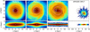 |
Fig. 1 Face-on (top row) and edge-on (bottom row) density map of the three models (from left to right) at the last snapshots, and the APOGEE DR17 sample used (right). The dashed black circle indicates the bar length, while the pink circle indicates the bar CR. They coincide for Model1. The black star indicates the location of the (simulated) Sun. Rotation is in the counterclockwise direction. The 2 × 2 kpc2 squares show the regions that will be studied in Figs. 4, 5, 8, and 10. Light blue indicates the left side of the bar, while orange indicates the right side of the bar. The solid squares are on the trailing side of the bar, while the dashed squares are on the leading side of the bar, although leading and trailing sides will not be differentiated in Sect. 5 (only one 2 × 2-kpc2 square per edge). The black and gray color indicates squares along the bar minor axis. These two squares will be stacked together and averaged in Sect. 4. |
2 Simulations
The three hydrodynamical simulations used in this work are the same as those used by Vislosky et al. (2024). They were chosen due to their similarity to the Milky Way, hosting both a bar and a spiral structure, and having similar disk properties. We examine their evolution over the last ~1.5 Gyr, long enough after the bar formation to avoid its effects on disk dynamics. For consistency, the models are called Model1, Model2 and Model3 as in Vislosky et al. (2024), whose aim was to reproduce the Gaia DR3 disk radial velocity field. Model1 and Model2, simulated in the cosmological context, were also used in Hilmi et al. (2020) to study fluctuations in bar parameters in relation to the periodic bar-spiral overlap. Model3 is an isolated galaxy, starting from a preassembled stellar disk, with gas and evolving with star formation and chemical evolution.
The first three columns of Fig. 1 show face-on and edge-on views of these models. The bars are aligned along the y=0 axis, and are X-shaped bars for Model1 and Model3, in contrast to Model2 which did not go through a buckling phase. The 2 × 2-kpc2 squares show the different regions which we studied in this work. The initial rotation curves of the three models, assumed to be flat, were  km/s,
km/s,  km/s,
km/s,  km/s. Despite the identical nomenclature with Vislosky et al. (2024), velocities were scaled slightly differently to match the current estimates of the MW rotation curve at the solar radius V0 = 229 km/s (Eilers et al. 2019), instead of V0 = 240 km/s. Similarly, distances were scaled so that the scale lengths of the three galaxies, initially
  kpc,
kpc,  kpc,
kpc,  kpc, would match current estimates of the MW scale length hd = 3.5 kpc (Bland-Hawthorn & Gerhard 2016). The resulting bar lengths for each model are
  kpc,
kpc,  kpc, and
  kpc. These values were derived using the Lcont method described by Hilmi et al. (2020), who define the true bar length only when the bar is not connected to any spiral, as the distance at which the background-subtracted-density drops to 50% of the maximum central density. The values used here are the time-median of the true bar lengths measured at each time the bar is disconnected from spirals over the last ~1.5 Gyr. Scaling of velocities and distances affect the mass of the galaxy according to GM ~ V2R (virial theorem).
For Model3, a preassembled disk and bulge, disk stars are indicated so their identification is straightforward. For the cosmological simulations however (as well as the observational data), applying cuts is necessary to isolate them. We considered stars to belong to the disk if (1) their birth |z0| and current |z| distance to the midplane are both less than 1 kpc, (2) their birth radii Rbirth are less than 15 kpc, (3) their current galactocentric radii R are less than 25 kpc, and (4) their eccentricity is less than 0.5 (to remove most stars trapped in the bar). Some disk stars have z > 1 kpc and were therefore removed from the analysis. However, including them did not affect our conclusions.
The meridional motion of stars can be approximated as the combination of a perfectly circular orbit at so-called “guiding radius” Rg (ideal, stable, symmetric case) and an epicyclic motion (radial oscillations) around Rg (Binney & Tremaine 2008). Thus, in the general case, two types of changes can affect the orbit: change of guiding radius, called radial migration, and/or an increase of epicyclic amplitude, called kinematic heating which can be related to an increase of the eccentricity of the orbit. For both simulations and the data, we estimated the stars’ guiding radii Rg and eccentricities e using the following expressions:
 (1)
(1)
 (2)
(2)
where R is the instantaneous galactocentric radius of the stellar particle, Vr and Vφ are the radial and azimuthal galactocentric velocities, and V0 is the rotation curve. Even though rotation curves are significantly increasing with radii in the centermost parts of disk galaxies, they quickly flatten and we therefore approximated V0 to a constant. As a result, guiding radii of the innermost stars could be underestimated. However, dividing V0 by 2 for stars at R < 3 kpc did not impact our conclusions. The eccentricity expression above was taken from Arifyanto & Fuchs (2006) for a flat rotation curve, as we also assumed in this work, and is reliable for eccentricities up to 0.5. As mentioned earlier, stellar particles with e > 0.5 were excluded from our analyses.
The APOGEE DR17 sample has a complex selection function as can be seen at least in the radial dimension in Fig. 1. Therefore, to properly compare the last snapshots of the simulations to the observations of APOGEE as will be done in Sect. 4.2, it is necessary to take these selection biases into account, as well as the measurement uncertainties. Uncertainties were introduced as Gaussians except for birth radii, for which the error strongly depends on age. We split the stars into 1 Gyr monoage bins, and fit the Rbirth error distributions from APOGEE DR17, which we then implemented for the same age populations in the simulations. For the selection effects, we used rejection sampling for the same age bins, to sample the simulations so that the radial distributions of each simulated age population would be the same as that of the corresponding observed populations. The number of stars for each age bin was kept equal to that in the APOGEE sample, which helps to address selection biases based on stellar evolutionary stage. Details are given in Appendix B.1.
2.1 Model1
The first cosmological model we used is model g2.79e12, a zoom-in version of a Milky Way-mass galaxy taken from the Numerical Investigation of a Hundred Astronomical Objects (NIHAO-UHD) simulation suite (Wang et al. 2015). First presented by Buck et al. (2018), it hosts both a bar and a spiral structure with -10% overdensity (ratio of the amplitude of the m=1, 2, 3 and 4 components to the m=0 Fourier component of the stellar density, see Vislosky et al. 2024). Hence it has been extensively used due to its similarity to the Milky Way (Buck et al. 2019; Buck 2020; Sestito et al. 2021; Lu et al. 2022, 2024; Buck et al. 2023; Wang et al. 2023; Buck et al. 2023). The simulation is based on the smoothed particle hydrodynamics solver GAS OLINE2. 0 (Wadsley et al. 2017). Star formation and feedback are implemented following the prescriptions of Stinson et al. (2006) and Stinson et al. (2013), who searched for simulation parameters that best reproduced the Kennicut-Schmidt law and the stellar mass–halo mass relation, respectively.
The simulation parameters can be found in Buck et al. (2019), the resolution is reported here: -5.2 × 10⁶ dark matter particles (5.141 × 10⁵ M⊙/particle), ~8.2 × 10⁶ stellar particles (3.13 × 10⁴M⊙/particle, total Mstar = 1.59 × 10¹¹M⊙), and ~2.2× 10⁶ gas particles (9.38 × 10⁴M⊙/particle, total Mgas = 1.85 × 10¹¹M⊙).
2.2 Model2
The second galaxy is model g106 of the zoom-in suite of 33 hydrodynamical simulations of Martig et al. (2012). The zoomin technique (Martig et al. 2009) consists in extracting the merger and accretion histories of a dark matter halo simulated in a cosmological context (here from Teyssier 2002), and then resimulating these histories at high resolution including baryons. The zoomed-in simulation used the Particle-Mesh code from Bournaud & Combes (2002, 2003). An extensive description of the simulation technique is given in Martig et al. (2012, 2014a), but we report some parameters here. Star formation is implemented using the Schmidt-Kennicutt law (Kennicutt 1998) with an exponent of 1.5 and a 2% efficiency. They set the threshold for star formation to 1 atom per cubic centimeter (i.e., 0.03 M⊙ pc-3). Similarly to Modell, this galaxy hosts both a central bar and a ~20-25% overdense spiral structure (ratio of the amplitude of the m=1, 2, 3 and 4 components to the m=0 Fourier component of the stellar density, see Vislosky et al. 2024). It has also been widely used for its resemblance to the MW (Kraljic et al. 2012; Minchev et al. 2013; Martig et al. 2014a,b; Carrillo et al. 2019; Hilmi et al. 2020).
The mass resolution for dark matter particles is 3 × 10⁵ M⊙, for stellar particles 7.5 × 10⁴ M⊙ and for gas particles 1.5 × 10⁴ M⊙ . The total stellar mass and dark matter mass within the optical radius (25 kpc) are ~4.3 × 10¹⁰ M⊙ and ~3.4 × 10¹¹ M⊙ respectively.
2.3 Model3
Model3 is an N-body simulation which contains a preassembled stellar disk, dark matter halo, and bulge with mass profiles as presented in Khoperskov & Gerhard (2022), to which a gas component was added, including star formation, feedback, and enrichment models. A full description was given by Vislosky et al. (2024). It simulates 3 Gyr of evolution of these preassembled components. Star formation is implemented with an efficiency of 0.05, and occurs in a gaseous cell when: (i) gas mass is > 2 × 10⁵ M⊙, (ii) the gas temperature is less than 100 K, and iii) if the cell is part of a converging flow.
This model contains 5 × 10⁶ dark matter particles of mass 1.25 × 10⁵ M⊙ and 6 × 10⁶ stellar particles of mass 7.5 × 10³ M⊙. The total gas mass is 1.5 × 10¹⁰ M⊙. Model3 also hosts both a bar and a ~20—25% overdense spiral structure (ratio of the amplitude of the m=1, 2, 3 and 4 components to the m=0 Fourier component of the stellar density, see Vislosky et al. 2024).
3 APOGEE DR17 sample
To compare the last snapshots of our simulations with MW observations, we used data provided by the catalog of the Sloan Digital Sky Survey IV (Blanton et al. 2017, SDSS-IV) APOGEE’s seventeenth data release (Majewski 2017; Abdurro’uf et al. 2022). Stellar parameters and abundances are derived from the data of two high-resolution spectrographs in both the northern and southern hemispheres using the APOGEE Stellar Parameters and Chemical Abundance Pipeline (Holtzman et al. 2015; García Pérez et al. 2016; Jönsson et al. 2020, ASPCAP). We used stellar kinematics from the astroNN catalog (Mackereth & Bovy 2018; Leung & Bovy 2019), and the uncorrected Sharma model ages from the distmass catalog (Imig et al. 2023; Stone-Martinez et al. 2024). We used the birth radii derived by Ratcliffe et al. (2025) for red giant branch stars that belonged to the disk (|z| < 1 kpc, e < 0.5, |[Fe/H]| < 1) with small uncertainties (Fe/H]err < 0.05 dex, unflagged [Fe/H], log10Ageerr;upper > 0). Stars with unreliable masses, and therefore ages, because they lie outside the distmass training set were also removed (flagged with BITMASK=2). These selections resulted in a sample of 161 994 disk stars, which is shown in the rightmost panel of Fig. 1.
4 Radial migration at the bar radius
4.1 Time evolution of stellar migration
A common way to visualize migration is plotting the change in guiding radius (∆Rg = Rg(t1) - Rg(t0 < t1)), versus the initial guiding radius (R0 = Rg(t0)) for a given time period ∆t = t1 - t0. From left to right, Fig. 2 probes the time evolution of the efficiency and direction of migration over a fixed time interval of ∆t = 0.1 Gyr. The (R0-∆Rg) plane is divided into 0.3 × 1.7 kpc2 bins for Modell and Model2 (top and middle panel) and 0.3 × 2.7 kpc2 bins for Model3 (bottom panel). The number of stars in those bins is given by the color bar, with contribution only from stars present throughout the whole period. Each panel corresponds to a particular time in the evolution of one of the three models. The times were chosen to be when the bar is either connected or disconnected to a spiral, as indicated in each panel. The black horizontal dashed line is at ∆Rg = 0 (i.e., no migration). Every particle above (below) this line migrated outward (inward). The black vertical solid line indicates the bar end, while the pink line indicates the corotation radius (CR). We note that the CR and the bar length overlap in Model1, revealing a fast bar.
A prominent ridge is visible at the bar end in all models, indicating strong ongoing migration at these radii, even though this is inside the bar CR for Model2 and Model3. Particularly striking in Model3, but also visible in Model2, is how the amplitude of this ridge varies with time. It is most pronounced when the bar connects to a spiral, and almost disappears when they disconnect. The ridge at the bar end remains prominent at all times for Model1. This model has a much weaker spiral structure, therefore the effect of the bar-spiral overlap is less visible here (but it is still present, see Fig. 5). We note that the (R0-∆Rg) plane, or its equivalent (L0-∆L), has been shown multiple times, but almost always for larger time intervals (e.g., Roškar et al. 2008; Minchev et al. 2011; Halle et al. 2018; Khoperskov et al. 2020). Using a time interval larger than a migration burst due to a specific event can result in blurring the structure (see Fig. C.1). This is the first time that such periodic fluctuations in the migration strength, measured as a change in guiding radius, have been shown.
Plotting ∆Rg against R0 as in Fig. 2 allows us to study how migration strength varies with radius, but not how it varies with azimuth, i.e., the angle relative to the bar major axis. Figure 3 shows two-dimensional histograms of the change in guiding radius, ∆Rg, as a function of azimuthal angle, φ, which has resulted in a time period ∆t = 0.1 Gyr for Model3 stars in different radial bins. For simplicity, most results in the rest of the subsection will focus on Model3. Differences with Model1 and Model2 will be discussed below. Figure 3 is the azimuthal expansion of the region between the two vertical black dashed lines in the bottom row of Fig. 2. Different columns show different guiding radius bins of width 2 kpc, spanning a region from 1.15 kpc (leftmost) to 7.15 kpc (rightmost). The bins overlap with one another by half the bin width. The bar ends are encompassed in the radial bin indicated in bold (second column), while its CR is at the border of the two radial bins indicated in pink (the two last columns). The two rows correspond to the first two columns of the last row of Fig. 2, that is times when the bar is either connected (first row) or disconnected (second row) to a spiral. We can see that out to Rg ~ 6 kpc a large number of stars initially located at the bar ends appear to mostly migrate slightly inward (∆Rg < 0). Although we removed high-eccentricity orbits (e > 0.5), this is likely due to them being trapped into the bar-supporting x1 orbits (e.g., Contopoulos & Papayannopoulos 1980), making it hard for them to escape the bar. Between the bar ends and along the bar trailing side however, stars migrate mostly outward to a variety of radii. Particularly, we note that stars initially at the bar radius (second column) can gain almost 3 kpc in radius in just 0.1 Gyr, reaching radii around 6 kpc, where they could once again be pushed away to, for example, the SNd by other migration inducing agents.
Looking more closely at the bar edges in Fig. 3, asymmetry can be noticed on the leading and trailing sides. ∆Rg seems to increase faster on the trailing side (solid lines, decreasing φ) than on the leading side (dashed lines, increasing φ), indicating larger migration on the former. This tendency was observed in other numerical works (e.g., Ceverino & Klypin 2007; Petersen et al. 2019), and its effects are also potentially seen in observed face-on barred galaxies (Neumann et al. 2024). It can be explained by the positive and negative torques applied respectively on the trailing and leading sides of the bar.
Furthermore, when the bar and the spiral are disconnected (bottom row of Fig. 3), the variations in migration along φ are the same for all radii, with minima along the bar axes. However, when looking at times of connection of the bar with a spiral (top row of Fig. 3), both the amplitude and phase of ∆Rg(φ) seem to change with radius. Going from innermost to outermost radii (left to right in the top row of Fig. 3), ∆Rg drops with radius, being mostly positive inside the bar radius (first column), and mostly negative outside the bar radius (from third panel). This trend is at the origin of the ridge at the bar radius seen in Fig. 2, where net migration is indeed outward inside the bar radius, and inward outside the bar radius. Moreover, the minima in ∆Rg are exactly at the bar ends for all radii when the bar is not connected to any spiral (bottom row). This is true only inside the bar radius, a region which spirals do not reach, when the bar is connected to a spiral (top left panel). At this moment of bar-spiral overlap, the minima in ∆Rg shift in azimuth as radius increases (from left to right in top column of Fig. 3), going from the bar azimuths and moving to the leading side of the bar. Therefore, Fig. 3 suggests that not only the torques vary with time as a result of bar-spiral overlap (causing stronger migration when connected), but torques seem to also shift in space, moving the zones of inward/minimal migration from exactly at the bar ends when bar and spiral are disconnected (bottom row), to along the leading side of the bar when bar and spiral are connected (top row). This behavior is verified across the 1.4 Gyr of evolution studied here, as can be seen in the online movie.
To visualize how migration strength along azimuth varies with time near the bar ends, we looked at the standard deviation of the distribution of ∆Rg along the initial azimuthal angle φ0 in different radial bins. Because mean migration is around 0 kpc, the standard deviation of ∆Rg indicates how far stars typically migrate, by ignoring the canceling effect of inward (∆Rg < 0) and outward (∆Rg > 0) migrators. We therefore defined the migration strength as the standard deviation of ∆Rg. Figure 4 shows the time evolution over 1.4 Gyr of migration strength, still over ∆t = 0.1 Gyr, for the radial bins of the different square regions shown in Fig. 1, but centered at increasing radii from top left to bottom right, following the radial bins of Fig. 3. Each curve in Fig. 4 is the migration strength associated with the same-color and same-linestyle squares. The gray curve is the mean migration strength along the two bar minor axis squares stacked together. The squares centered at the bar radius are those shown in Fig. 1 and the corresponding migration strength evolution is the third panel of the first row, where the radial bin is indicated in bold. The other panels correspond to a horizontal (vertical) translation of these squares for the light blue and orange (gray) curves. First comparing the leading and trailing sides of the bar, we notice that out to the bar radius (up to third and fourth panels), regions along the trailing side of the bar show more migration than along the leading side of the bar, as noticed in Fig. 3. This is no longer true from the CR, around 5 kpc (bottom left panel). The gray curve is almost always lower than the colored curves, indicating less variety in migration along the bar minor axis (all minor axis migrators reach more similar radii). Showing the two opposite sides of the bar minor axis separately did not change this trend. Despite these differences, all curves show periodic fluctuations on similar frequencies in the migration strength around the bar up to just outside the bar radius (top right panel), generalizing observations from Figs. 2 and 3 to a longer timescale. Around CR, significant fluctuations are still present, as strong as at the bar radius. This could be explained by the fact that the bar-spiral overlap also makes the bar pattern speed oscillate, which in turn affects its resonances as well (Hilmi et al. 2020). Indeed, as one nears CR, many higher order resonances are encountered. They could also be at the origin of the extra small wiggles in the minor axis (gray line) at R = RCR in Fig. 4, along which the L4 and L5 points lie. Outside the CR, fluctuations in std(∆Rg) are still present, but are much less regular as another migration agent must have taken over. The slight decrease at all radii of the peaks in migration strength with time is likely because the disk gets hotter and thus less sensitive to perturbations like the bar and the spiral. We note that these oscillations in guiding radius could also be the result of libration around the fourth and fifth Lagrange points, as was shown to occur around the bar corotation (Ceverino & Klypin 2007; Binney & Tremaine 2008; Haywood et al. 2024; Khoperskov et al. 2025). This effect, however, does not produce a continuous increase in ∆L (or ∆Rg) with time (see e.g., Minchev & Famaey 2010, Fig. 2). In contrast, we find that the mean ∆Rg is overall positive (see Fig. 5), suggesting that migration is indeed happening, on top of libration.
Hilmi et al. (2020) showed that the bar appears longer when it overlaps with a spiral mode. To verify that the boosts in migration seen in Fig. 4 are related to bar-spiral overlap, we compared them with the time evolution of the bar length. Focusing back on the bar region, in Fig. 5 we present several statistics of the population of stars found at a time t in one of the 5 regions around the bar shown in Fig. 1 : the standard deviation of their ∆Rg in ∆t, which we call the migration strength ; their mean ∆Rg in ∆t; and the mean Rg that their 5% most extreme migrators reach after ∆t. Figure 5 compares the time evolution of these quantities to the bar length evolution for our three models. Each column corresponds to one model as indicated in the top panels, while each row shows a different quantity. As for Fig. 4, each curve represents the migration statistics of the corresponding region. The top rightmost panel is the same as the top second-to-last panel of Fig. 4. Curves in the three first rows were smoothed with Gaussian kernels of standard deviation 5 Myr, 3 Myr and 7 Myr from left to right respectively. Bar lengths curves were smoothed with Gaussian kernels of standard deviation 8 Myr, 9 Myr, and 17 Myr. Smoothing widths are functions of the time resolution of each simulation. Since the bar length measurements are more susceptible to noise than the migration statistics (which are somewhat already averaged), a stronger smoothing was applied to bar length measurements.
All the models show oscillations, but with different frequencies. Model1 has a faster bar, and exhibits more rapid oscillations in its migration statistics for all azimuth around the bar, while the slower bars of Model2 and Model3 correlate with slower fluctuations. This highlights the importance of the bar in producing these migration bursts. We also note the stronger migration in Model3, which exhibits higher values for all migration statistics than in Model1 and Model2. These galaxies, simulated in the cosmological context, could be hotter because of their interaction with other objects, making them less sensitive to bar and spiral perturbations. Moreover, Model1 has a weaker spiral structure than Model2 and Model3, and its oscillations in migration strength have a lower amplitude (~0.06 kpc variation versus ~0.2 kpc for Model2 and ~0.6 kpc for Model3). We also see that peaks associated with the different azimuths coincide quite poorly in time for Model1, compared to Model2 and Model3. This can explain why Model1 did not show any variation in the amplitude of the ridge at bar radius in Fig. 2, since, for one radius, the variations at the different azimuths can cancel one another out over time.
The std(∆Rg) (first row in Fig. 5) is higher for trailing sides (solid) than leading sides (dashed) in Model2 and Model3 particularly, suggesting more migration there as seen in Figs. 3 and Fig. 4. This is less clear for Model 1, although we do find some significant difference between leading and trailing sides in the mean change in guiding radius. The mean change in guiding radius (second row) allows us to study the direction of migration. The gray curve, representing the bar minor axis, is above zero at all times, indicating a net outward migration. This confirms that these oscillations result from the permanent redistribution of angular momentum, and not pure libration. On the contrary, the leading sides of the bar (dashed) produce negative mean ∆Rg in all models, again hinting toward negative torques applied on this side of the bar. The trailing sides of the bar (solid light blue and orange) seem to oscillate around zero (except for Model2 where mean(∆Rg) < 0 kpc), suggesting both positive and negative torques successively applied on the stars. The fact that stars on the trailing sides of the bar migrate further away than those on the leading side is confirmed by the mean guiding radius reached by the 5% most extreme migrators in ∆t = 0.1 Gyr (third row) in all models. This final radius is much higher at all times for the trailing sides, reaching up to 6 kpc. On longer timescales, the stars could even reach larger radii, thus entering the SNd.
The last row of Fig. 5 shows the bar half-length time variations of all models. The bar length was calculated using the Lcont method described by Hilmi et al. (2020), defining the bar length as the minimum distance at which the background-subtracted density profile drops by 50% compared to the radial mean density along the major axis of the bar. The bar length fluctuates as shown by Hilmi et al. (2020) and Vislosky et al. (2024). The peaks in Rbar correspond to times when the bar and the spiral are connected. Their frequency coincide quite well with the boosts in the migration strength of all models (first row), and in the mean change in guiding radius along the bar minor axis and the trailing side of the bar, despite these quantities being measured independently and with very different methods. Hilmi et al. (2020) performed a Fourier decomposition of this model, and find a reconnection time of Trec ∼ 60 Myr between the bar and the m = 2, 3 and 4 spiral modes. Over a timescale of 1.3 Gyr as used here, this should result in around 21 peaks, which is very similar to the number of peaks found here, as indicated in the top and bottom panels of Fig. 5. Peaks were counted using the find_peaks function from the python library scipy, which identifies peaks as local maxima by comparison of neighboring values. Similarly for Model2, Hilmi et al. (2020) find a reconnection time of Trec ∼ 105 Myr for the bar and the m = 2, 3 and 4 spiral modes. Over the 1.4 Gyr represented here, this would mean around 13 peaks in migration and bar length. Our results are indeed very close to this result, corroborating the link between bar-spiral coupling, and regular migration boosts. In Model3, the bar length and migration peaks are much smoother, and their time offset quite small, so their correlation is more obvious. Since all bar parameters, length, strength, and pattern speed, oscillate as a result of this regular coupling, the migration fluctuations can be linked to both the periodic fluctuations in density at the bar ends, when the bar and a spiral arm physically overlap, and from the bar-spiral resonance overlap creating a stochasticity in this region of phase space (Minchev & Famaey 2010). These two processes most likely work in unison.
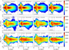 |
Fig. 2 Change of guiding radius over ∆t = 0.1 Gyr vs. initial guiding radius for Modell, Model2, and Model3 stars from top to bottom. Each column represents a different initial time, which increases from left to right as indicated in the top of each panel. These times were chosen to be at moments when the bar and the spiral are connected or disconnected. The dashed horizontal black line shows ∆Rg = 0, (i.e., no migration). All points above (below) this line represent stars that migrated outward (inward). The solid black line indicates the bar length, while the pink line indicates the bar corotation radius. They coincide for Model1. The vertical dashed lines in the bottom panel indicate the radial range over which the azimuthal variations of migration are investigated in Fig. 3. Panels corresponding to bar-spiral connection times show a very prominent ridge at the bar end, while this ridge is much less pronounced at bar-spiral disconnection times, except for Model1 where the weak spirals diminish this effect. |
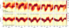 |
Fig. 3 Two-dimensional histograms of the change in guiding radius over ∆t = 0.1 Gyr with respect to the initial azimuthal angle for stars in Model3 initially in different 2-kpc-wide radial bins. Each column is for a different radial bin, going further out from left to right as indicated in each panel. The bar ends (Rbar = 3.15 kpc) are encompassed in the second column and are indicated by the bold text, while the corotation (RCR = 5.3 kpc) is at the border of the fourth and fifth bins and is indicated in pink. The left and right sides of the bar are shown by the light blue and orange vertical dotted lines, respectively. The solid lines indicate the trailing side of the bar edges, while the dashed lines indicate their leading sides. Those lines are located at the edge of their associated square regions from Fig. 1. The different rows represent the same quantities at different times in the disk evolution. They are the same times as those in the first two columns of Fig. 2, and thus show a time at which the bar is connected to a spiral (first row), as well as a time when the bar is not connected to any spiral (second row). The (φ-∆Rg) plane of Fig. 3 is divided into 5° × 0.1 kpc bins and the number of stars in those bins is given by the color bar, with a contribution only from stars present throughout the whole period. The full temporal evolution over the last 1.4 Gyr of evolution is available as an online movie. |
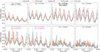 |
Fig. 4 Time evolution of migration strength from different galactic disk radii in Model3. In each panel, the different curves correspond to the migration strength (i.e., how far stars found in this region at some time, t, migrate after ∆t) of stars originally found in each of the squares shown in Fig. 1. Light blue and orange indicate the left and right sides of the bar, respectively, while solid and dashed represent the trailing and leading sides of the bar, respectively. The gray curve is the mean migration strength along the bar minor axis (i.e., the two gray squares of Fig. 1). From left to right, these squares are shifted horizontally (light blue and orange) and vertically (gray), along the bar major and minor axis, respectively, to probe different radii. |
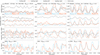 |
Fig. 5 Time evolution of different migration statistics compared to bar length time evolution, for the three models (from left to right). Different azimuths around the bar radius are scanned using the six 2 × 2 kpc2 square regions shown in Fig. 1. The gray curve is the mean statistical quantity over the two squares placed along the bar minor axis. Again, blue and orange curves represent the left and right sides of the bar, respectively, while solid and dashed lines stand for the leading and trailing sides of the bar, respectively. The number of peaks of these curves is indicated as N̄peaks in the top and bottom panel; N̄peaks is the mean Npeaks over the different curves. First row: standard deviation of the change in guiding radius over ∆t = 100 Myr experienced by all stars located in the six different square-shaped regions. Second row: same as top row, but for the mean change in guiding radius, which slows the net angular momentum transfer. Third row: mean guiding radius after ∆t = 100 Myr for the 5% stars that migrate the most. Last row: time evolution of the bar half-length. The peaks correspond to moments when the bar is connected to a spiral arm. The maxima in the migration strength, or their frequency, coincide with those of the bar half-length, which indicates that they are a result of the interaction between the bar and spiral arms. |
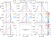 |
Fig. 6 Birth radius distribution of stars found at the solar radius today (inside the gray vertical strip) of, from left to right, the two cosmological models Model1 and Model2, and the APOGEE DR17 red giant sample. The black curves are for the whole sample. In the top row, the blue and yellow curves highlight stars found today on orbits with e < 0.2 (cold) and 0.2 ≤ e < 0.5 (warm), respectively. The percentages that warm and cold stars born inside Rbar represent in the SNd are indicated in the top right of the panels for each galaxy. In the middle row, Rbirth distributions are shown for different monoage populations. From purple to red, stars get older and older, as indicated in the color bar. In the bottom row, Rbirth distributions are shown for different metallicity bins, blue and red representing metal-poor and metal-rich stars, respectively as indicated in the color bar. |
4.2 Impact on the solar neighborhood
We showed in Figs. 3 and 5 that stars in the vicinity of the bar could migrate out to almost twice their radius in just 100 Myr, thus potentially later ending up in the SNd and polluting the local chemistry. To better quantify this effect, we studied the birth radius distribution of stars found today in the SNd of our two cosmological models and the APOGEE data. Model3 is a preassembled disk, and can therefore not reproduce the age distribution found in the data. Moreover, it is isolated, and so less realistic than cosmological models. Hence we did not consider it in this subsection.
Figure 6 shows the distribution of birth radii of stars found today in the SNd for, from left to right, Model1, Model2, both biased with measurement errors and according to APOGEE monoage radial distributions, as explained in Appendix B.1, and the APOGEE DR17 red giants sample. The SNd stars are defined as stars with current radius at most 0.5 kpc away from the Sun’s radius (R⊙ = 8.125 kpc). This region is indicated by the gray band in the three rows of Fig. 6. In the top row, we show two curves for stars with two different orbital eccentricities today. The blue and yellow are respectively for e < 0.2, and 0.2 < e < 0.5. For simplicity, we call them ‘cold’, and ‘warm’ orbits (‘hot’ orbits would have e ≥ 0.5). The black dashed vertical line indicates the bar radius of each model. For the MW, we used Rbar = 3.5 kpc, in accordance with recent measurements (Lucey et al. 2023; Zhang et al. 2024). Distributions vary from model to model. Model1 shows a bimodal Rbirth distribution, with a large fraction of stars, both cold and warm, coming from about 1 kpc inside the solar radius, and another significant population born just inside the bar radius. The distributions are smoother in Model2 and in the data, with most stars coming from just inside or at the solar radius, with a slow decrease toward inner birth radii, and a faster one toward the outer disk. This indicates more outward migration than inward migration. The proportions of SNd stars today on cold and warm orbits, and born inside the bar radius go from 1.75 to 8.5% for cold stars, and from 3.5 to almost 18% for warm stars. Model2 is the model with the least amount of migrators originating from the bar. These differences could arise from different reasons. First, Model1 has a shorter reconnection time than Model2 (see Hilmi et al. 2020), which means that the bar-spiral overlap migration mechanism has had more occasions to send stars away, therefore contaminating the SNd even more. Moreover, the spiral structure in Model1 is weak compared to Model2, which can explain why more stars come from the bar rather than from the disk. Furthermore, the majority of stars born at the bar radius in Model1 are on warm orbits. Since the simulated SNd samples were selected based on stellar instantaneous radii, many of these warm stars could be on their apocenters, with their guiding radius actually residing inside the solar radius. Finally, Model1 experienced a massive merger about 4 Gyr ago (Buck et al. 2023), which must have heated stellar orbits as well as caused large-scale migration. In contrast, the MW’s last 8 Gyr have been quieter (Martig et al. 2014a,b; Haywood et al. 2018; Helmi et al. 2018; Di Matteo et al. 2019). Despite these differences, a significant portion of stars from all the models come from inside the bar and are found today on cold and warm orbits.
To further characterize the stars found in the SNd, we show in the middle panel of Fig. 6 the same histograms, but with curves colored by age. The black curve represents the Rbirth distribution for all stars found in the SNd today. In the middle row of Fig. 6, each colored curve is for an age bin of width ∆age = 2 Gyr, as indicated in the color bar. Since the oldest stars are rare, the oldest bin contains all stars older than 10 Gyr to allow for a similar number of stars as in the other age bins (see proportion of each age population in the legend of each panel). The youngest stars (purple) were born mainly in the SNd, because their young age has not yet allowed them to migrate significantly. In Model2 (middle column), some stars born 2–4 Gyr ago seem to have migrated inward, possibly from an encounter with a satellite or outer spiral resonances. Despite this peculiarity, as age increases, the peak in the Rbirth distribution overall shifts to inner radii as predicted by an inside-out formation scenario. It is therefore mostly the old stars that come from inside the bar.
In the bottom row of Fig. 6, we show the birth radius distributions of different monometallicity populations. From blue to red, the metallicity increases as indicated in the color bar. We do not have metallicity for Model2, hence the empty panel. In both the data and Model1, as birth radius decreases, stars get more and more metal-rich. In particular, stars born inside the bar radius (vertical black dashed line), are mainly metal-rich. This is in good agreement with several other works attributing the origin of the super-metal-rich stars to the inner Galaxy only using chemistry and orbital properties from a variety of Galactic surveys, with some relating it to bar evolution (e.g., Kordopatis et al. 2015; Feuillet et al. 2018; Khoperskov et al. 2020; Haywood et al. 2024; Nepal et al. 2024).
Figure 7 shows in particular the age distribution of the stars born inside the bar and found today in the SNd on cold (blue) and warm (yellow) orbits. This is the age distribution of the stars represented by the solid part of the blue and yellow curves in the top row of Fig. 6. As suggested in the middle row of Fig. 6, most of them are old stars, with ages peaking at around 10 Gyr in the simulations, and more around 8 Gyr in the MW. This is not a surprising result since they had the most time to migrate and travel larger distances. In future work, we plan to investigate the time at which those stars migrated to disentangle the possible causes for their migration: internal mechanism, or a major merger event, like Gaia-Sausage Enceladus for the MW (Belokurov et al. 2018; Helmi et al. 2018; Haywood et al. 2018), which should have pushed away a large number of stars. The older stars that did not migrate because of an interaction with an external perturbation must have migrated due to internal processes, like a bar-spiral overlap as studied in this paper, due to a slowdown of the bar (Khoperskov et al. 2020), or an overlap of bar CR and spiral inner Lindbald resonance (Minchev et al. 2011) (see discussion in Sect. 6.1). In all galaxies, we also see a long tail of younger stars, which must also have migrated from these internal processes. Figure 7 also shows how the distribution of cold and warm extreme migrators in each galaxy is quite different, with a majority of cold stars in the MW, but a larger proportion of warm stars in the two simulations. As mentioned above, Model1 had a late merger around 4 Gyr ago (Buck et al. 2023), much later than the last merger of the MW, which must have heated stars. Moreover, simulated galaxies often have hotter stars compared to observations (Sellwood 2013; Ludlow et al. 2021, 2023; Wilkinson et al. 2023), which could explain this difference. Despite that, we note that all these stars are on rather cold orbits today (e < 0.5). Stars with e > 0.5 were removed, but represented a negligible fraction in the simulated SNds (8% of total SNd stars in Model1, and less than 1.5% in Model2). Since orbit cooling is unlikely (but marginally possible under the effects of the bar slowing down, see Khoperskov et al. 2020), most stars must have migrated without significant heating, as those would be preferentially selected (this is known as “provenance bias”, see Vera-Ciro et al. 2014).
To summarize this section, we found periodic oscillations in the migration strength near the bar radius of three different models, one isolated and two in a cosmological context. These oscillations happen on timescales of the bar-spiral beat frequency. We interpret this correlation as a new mechanism for migration, produced by bar-spiral interaction, similarly to the mechanism of transient spirals since the bar radius experiences a time-varying potential due to its interaction with various spiral modes. Oscillations are seen from the bar ILR to outside its CR. Migrators from bar-spiral interactions travel longer distances when they start from along the minor axis of the bar than along the bar major axis, where a lot of stars are trapped in the bar. In addition, we see stronger outward migration for stars located at the trailing edge of the bar compared to those located at the bar leading edge, which we interpret as torques of opposite sign applied along these two sides of the bar, in accordance with previous studies. Mean migration is positive for stars initially along the minor axis of the bar, confirming that libration is not sufficient to explain those guiding radius oscillations. The 5% most extreme outward migrators reach radii of 4 to 6 kpc in 100 Myr, suggesting that stars born at the bar radius can reach the SNd when given a bit more time.
To investigate the impact of extreme migrators in the SNd, we compared the simulated SNd at the last snapshots of our cosmological models to APOGEE DR17 data. Looking at the birth radius distribution of these SNd stars, we find that 5–23% of them were born inside the bar radius, are still on relatively cold orbits, and are mostly old and metal-rich.
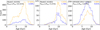 |
Fig. 7 Age distribution of stars found at solar radius today but born inside Rbar. The two curves follow the same line style and color code as in the top row of Fig. 6: solid for stars born inside Rbar, blue and yellow for kinematically cold and warm stars, respectively. The percentages in the legend are the proportion each eccentricity population with Rbirth < Rbar represents in the whole solar radius sample indicated in gray in Fig. 6. In the three cases, both the cold and warm distributions are mostly old (10 Gyr in the models, 8–9 Gyr in the data) with a tail to younger ages. |
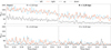 |
Fig. 8 Modell star formation temporal evolution in 2 × 2 kpc2 square regions centered at increasing radii from left to right and top to bottom, spanning radii from 2.25 kpc to 5.25 kpc. The squares of the leading and trailing sides of the bar, shown in Fig. 1, are merged into one square per edge of the bar centered on (x, y) = (±R, 0), light blue and orange indicating the left and right side, respectively. The upper and lower edges of the bar minor axis are differentiated, using black and gray, respectively. The regions at the bar ends show i) lots of fluctuations, ii) more star formation than along the bar minor axis until just outside the bar radius. |
5 Star formation at the bar radius
We have shown in the previous section that when a bar end and a spiral arm overlap, they create a transient overdensity and cause bursts of radial migration with frequency on the order of the bar-spiral beat frequency, typically 60–250 Myr, depending on the bar pattern speed. In this section, we investigate whether the star formation rates at the interface radius also follows the rhythm of this periodic bar-spiral connection. We focused on four squares centered on the bar half-length radius at the four edges of the bar axes. They have the same 2 × 2 kpc2 size as those used in the previous section (see Fig. 1), but the light blue and orange squares at each side of the bar have been combined into one square per edge, centered at (x, y) = ±(Rbar, 0). We therefore removed the distinction between leading (solid) and trailing (dashed) sides of the bar, because they did not show any difference in the star formation history. Moreover, we do not use Model3 in this section because SF is low in the region of interest, and therefore very noisy.
We report the number of stars born inside those four regions in Fig. 8 at each snapshot of Model1. All curves were smoothed with a Gaussian kernel of standard deviation 10.35 Myr. The different panels are obtained by moving the squares along the same axis, therefore scanning increasing radii from top left to bottom right. The highest SF is found in the innermost bin (top left panel) along the bar axis (light blue and orange), which is actually entirely inside the bar. There is clearly much less SF along the bar minor axis. Although at this radius, the minor axis squares might also sit inside the bar envelope, bar density decreases faster vertically than horizontally, for both stars and gas, explaining lower SF activity. This does not necessarily mean that the bar ends are more efficient at forming stars than regions on the bar minor axis. Looking at the mass of gas particles in these two regions is the only way to compare their SFE. The first column of Fig. 9 shows the time evolution of the surface gas density and the SFE in the four regions of interest centered on Rbar in Model1. Results at other radii follow the same trend as Nstars , but are not shown here. The top panel shows that there is only about 20% less gas at the minor axis of the bar, whereas the bottom panel reveals a much higher star formation efficiency at the bar major axis (more than 200% greater than at the minor axis). Therefore, the higher number of newly born stars at the bar ends seen in Fig. 10 can be explained marginally by a larger quantity of gas available, but mainly because this gas is much more efficient at turning into stars. We find the same tendency in Model2, although not as strong, as we can see in the right column of Fig. 9, where the major axis has 40% more gas than the minor axis, and has about 65% more SFE. In the MW, this could be due to orbital crowding at the bar ends, which enhances the probability of cloud-cloud collisions and leads to increased SFE, as shown by Renaud et al. (2015), although the distribution of SF within the bar radius seems to depend on galaxy properties (Fraser-McKelvie et al. 2020; Díaz-García et al. 2020; Maeda et al. 2023). We also note the recurring anticorrelation between SFE at the left and right ends of the bar, especially in Model1.
Also notable in Fig. 8 are the rapid fluctuations in SF, present along both bar axes. In the radial bin centered on the bar radius (top right), the global tendency is the same as inside the bar radius, with more extreme star formation along the bar major axis, and rapid fluctuations. However, the overall star formation is lower at these radii (bar radius) than in the previous bin (inside the bar). This is in agreement with Géron et al. (2024), who showed that for barred galaxies from the SDSS-IV MaNGA survey, star formation in the innermost regions was very high, decreased along the bar, and increased a little again just before reaching the bar radius. According to their observation, star formation in the innermost parts remains much higher than at the bar radius, which again appears consistent with our Fig. 8 (see also Di Matteo et al. 2013; Fragkoudi et al. 2018; Neumann et al. 2024). At 4.25 kpc, the difference between bar major and minor axis starts decreasing, and completely disappears from 5.25 kpc onward as they are away from the bar ends and outside CR. Outer radii are not shown here, but we did check they followed the same trend.
To see if the fluctuations in SF at the bar radius correlate with the bar-spiral overlap, we compared them with the fluctuations in the bar length in Fig. 10. We show results for both Model1 (left column) and Model2 (right column). The top row shows the star formation history at the bar radius (top left panel is therefore the same as the top right panel of Fig. 8), while the bottom row shows the bar length measured with the Lcont method of Hilmi et al. (2020). SF curves for Model2 were smoothed with Gaussian kernels of standard deviation 12.15 Myr. Model1’s fast bar is characterized by a high frequency in both the bar length and star formation fluctuations. Model2 having a slower bar, fluctuations have a longer period, already revealing the importance of the bar pattern speed on star formation. As in Sect. 4, we counted the number of peaks in these two quantities, as indicated in the corresponding panels. SF in Model1 has 21 and 22 peaks at the left and right side of the bar respectively. This is consistent with Trec = 60 Myr found in Hilmi et al. (2020), which supports the correlation between SF and bar-spiral overlaps. For Model2 (right), four main peaks are seen both in bar length and star formation, at times 12.5 Gyr, 12.8 Gyr, 13.1 Gyr and 13.5 Gyr, i.e a peak every ~325 Myr. This corresponds to the reconnection time of the bar with the m=1 and the fast m=3 spiral modes reported in Hilmi et al. (2020). Extra higher frequency peaks are also present, suggesting the presence of other likely weaker spiral modes. Indeed, we find a total number of peaks in star formation at each end of the bar of around 13, which is consistent with the reconnection time Trec ~ 105 Myr for the m=2, 3 and 4 spiral modes, as shown in Sect. 4. This supports the fact that the relation between bar-spiral coupling and star formation in the late epochs of galaxy evolution is not simulation-dependent. SF is enhanced by a factor of 3 in Model1 and 4 in Model2 when the bar and a spiral arm overlap, compared to when they disconnect.
It is important to note that the number of peaks is sensitive to the smoothing width. Indeed, SF was smoothed with wider Gaussian kernels than the bar lengths (10.35 Myr vs 8.28 Myr for Model1, 12.15 Myr vs 9 Myr for Model2). Smoothing SF with the same kernels used for bar lengths, as exepected, resulted in a larger number of SF peaks. These extra peaks could be due to weak spiral modes, that are not strong enough to affect our bar length measurements, but strong enough to produce star formation. We decided to smooth the SF with slightly larger kernels to reduce this effect. Despite this dependence on smoothing, it is clear that the galaxy with the shortest bar-spiral reconnection time produces more frequent starbursts, and the most prominent four peaks in Model2 found in star formation and bar length, as well as in migration strength, show a clear correlation with bar-spiral interaction.
Finally, we also note that peaks in star formation do not necessarily happen simultaneously at the two sides of the bar (e.g., at 12.6 Gyr in Model1, or 13.2 Gyr in Model2) which must be due to a nonbisymmetric spiral structure as was indeed found in the Fourier spectral decomposition done by Hilmi et al. (2020). In the MW, the distribution of star formation appears asymmetric in the inner Galaxy. The WISE Catalog of Galactic HII Regions (Anderson et al. 2014) is a compilation of all known and candidate massive star forming regions identified by their Wide-Field Infrared Survey Explorer (WISE) infrared morphologies and correlated with radio continuum and spectroscopic ionized gas observations. Armentrout et al. (2021) showed that most, if not all, HII region candidates in the WISE Catalog are bonafide HII regions, even if they lack a spectroscopic ionized gas detection. The first Galactic quadrant, which includes the near end of the bar, contains about 50% more HII regions and HII region candidates than the fourth quadrant, which contains the far end of the bar. Considering only the ends of the bar (north: (30 ± 2.5)° ; south: (-15 ± 2.5)°), the asymmetry is exaggerated: there are twice as many HII regions and HII region candidates in the wedge containing the northern end of the bar compared to the wedge containing the southern end of the bar (see Fig. 11). This can be explained by the presence of an odd spiral mode, if only one end of the bar is connected to a spiral arm, thus experiencing a burst of SF, while the other side is not (or if one end of the bar is connected to more arms than the other, in the case of a superposition of several spiral modes). A nonbisymmetric spiral structure in the MW is also consistent with Khalil et al. (2025), who recently showed that several features in the inplane motions of disk stars, of which moving groups and phase-space ridges, could be obtained from having an axisymmetric gravitational potential, to which a bar, and an m=2 and m=3 spiral modes are added. We also note that, as argued by Nguyen Luong et al. (2011), the near end of the Galactic bar, which is believed to meet the Scutum-Centaurus arm, hosts W43, a molecular cloud complex considered one of the most extreme star forming region of the MW. This mini-starburst region, as dubbed by Motte et al. (2003), could have SFE of 25%/yr, and was extensively studied for its outstanding star formation activity (Bally et al. 2010; Motte et al. 2018; Kohno et al. 2021; Nony et al. 2023, and references therein). In this region, bar-spiral connection could be enhancing star formation by triggering shocks, cloud-cloud collisions or colliding flows, as reported in the literature (e.g., Louvet et al. 2016; Sofue et al. 2019; Lin et al. 2024).
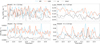 |
Fig. 9 Mass of gas (top panel) and star formation efficiency (bottom panel) across time in Model1 and Model2 from left to right, for the four regions used in Figs. 8 and 10. There is slightly less gas along the minor axis of the bar compared to its major axis, which partially explains the lower number of newly born stars in the former. However, the main reason for the higher number of newly born stars at the bar major axis is the much higher SFE, as seen in the bottom panel. The time evolution of SFE at the two sides of the bar (blue and orange) often anticorrelates, which suggests the presence of a nonbisymmetric spiral structure. |
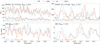 |
Fig. 10 Comparison of the time evolution of the star formation in the four square regions used in Fig. 8 (top row) to that of the bar half-length (bottom row), for Model1 and Model2 (left and right column, respectively). Peaks in Rbar correspond to the times of bar-spiral connection. The frequency of these bar length peaks coincides with the frequency of the starbursts seen in the top panel (see number of peaks Npeaks in each panel), which suggests their correlation with the periodic bar-spiral overlaps. Starbursts do not always happen at the same time at the two ends of the bar. |
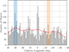 |
Fig. 11 Distribution of HII regions in the Milky Way as a function of galactic longitude. The red curve is a kernel density estimate of the histogram, in black, which shows data from the WISE catalog. Regions shaded in blue and orange are in the direction of the near and far side of the bar, respectively. There are twice as many objects in the direction of the near end of the bar compared to that of the far end of the bar. |
6 Discussion
As we have shown throughout Sect. 4, the bar-spiral overlap acts like a transient overdensity and causes radial migration from the bar ILR out to its CR. This is, to a first approximation, quite similar to the process of transient spirals presented by Sellwood & Binney (2002). In the presence of a rotating nonaxisymmet-ric pattern, horseshoe (HS) orbits appear in the rotating frame, near the CR of the pattern (Binney & Tremaine 2008). Sellwood & Binney (2002) argued that transient spirals that survive long enough to (1) trap stars in these HS orbits, and (2) allow stars to go from one side of the CR to the other only once, can produce permanent changes in the individual stellar angular momenta. However, such short-lived spirals struggle to explain the large amount of migration observed in galactic disks, especially when comparing with the amount of heating per unit migration (see Hamilton et al. 2024).
Comparetta & Quillen (2012) proposed that the interference of multiple spiral density waves, that can result in short-lived mass clumps, can be an alternative to transient spirals. They showed that, to produce efficient migration, the lifetime of interference peaks of the two interfering waves should be shorter than the stellar rotation period at the radius of interest. This scenario is very similar to the bar-spiral overlap, which also gives rise to such interference peaks, as inferred by the fluctuations of the bar length (Fig. 5) and the gas mass near the bar ends (Fig. 9). We therefore expect that the bursts of migration that we observe to occur on the bar-spiral beat frequency timescale (corresponding to the lifetime of an interference peak) can be modeled in the same way.
6.1 Migration mechanisms of the most extreme migrators
In Sect. 4.2, we saw that most of the extreme migrators (Rbirth < Rbar) found in the SNd must have migrated without significant heating. The two known migration mechanisms that are capable of migrating stars from the very inner regions to the SNd while maintaining their cold orbits are the bar slowdown of Khoperskov et al. (2020) and the bar-spiral interaction mechanism presented in this paper. In the N-body simulation used by Khoperskov et al. (2020), the slowdown of the bar is significant only during the first Gyr of its formation, at a rate of  as we can deduce from their Fig. 1 (see also Haywood et al. 2024). In their simulation, the bulk of the corresponding migration also occurs in the first couple of Gyr following the bar formation (see their Fig. 3). The migrators associated with this mechanism should therefore be at most 2 Gyr younger than the bar (or older than the bar), putting an age lower limit on bar-slowdown migrators. The younger migrators from the bar region must therefore have migrated due to the interaction of the bar and the spiral, as we have shown in this paper. This constrains the migration mechanism for the youngest migrators, but cannot constrain it entirely for the older migrators, since observations cannot provide the time evolution of stellar radii, but merely the current positions, the age and birth radii of stars. In principle, this information is accessible from simulations by tracking stars from their birth to the current time, therefore telling us when they migrated. However, we leave this analysis for future works. What we can deduce from this work, is that most stars migrate without significant heating, and that bar-spiral interaction is a good candidate to explain the arrival in the SNd of young (and some old) and cold stars that were born at the bar radius. We also note that other studies have investigated the impact of the bar slowdown on the dynamics of stars. Notably, Chiba et al. (2021) and Zhang et al. (2025) find that the Milky Way had chemodynamics consistent with a bar slowing down at a rate of
  , which can create efficient and continuous migration for stars trapped at the (sweeping) bar CR. Model2 and Model3 have indeed similar bar slowdown rates (see Fig. A.1). This suggests that the bar slowdown could still have a significant impact in these two galaxies, and could still be active in our Galaxy. With such (constant) slowdown rates, stars from the bar radius (Rbar = 3.5 kpc, which is where the CR could have been when the bar formed) reach the solar radius (R⊙ = 8.2 kpc) in 5.8 Gyr (using η with Ωb = V0/RCR). Hence, even if the bar slowdown is still significant today and has been since the bar was formed, it cannot explain the migration of stars younger than about 6 Gyr from inside the bar radius out to the solar radius. Note however that the slowdown of the bar might not be constant over its lifetime, as seen in several simulations with self-consistently formed bars (Debattista & Sellwood 2000; Athanassoula 2003; Valenzuela & Klypin 2003; Petersen et al. 2019; Khoperskov et al. 2020; Haywood et al. 2024). Moreover, the bar in Model1 is actually speeding up in the last 1.5 Gyr as we can see in Fig. A.1, which should theoretically lead to inward migration through the sweeping of resonances. We do not see any significant traces of such mixing, although the speeding up rate could be too small to efficiently move anything.
6.2 Interplay of migration boosts and star formation bursts
Both the migration boosts and the star formation bursts happen on the timescale of the bar-spiral beat frequency, but we have treated the two phenomena separately in this paper. It is however possible that their interplay could play a distinctive role in the chemodynamical evolution of galaxies. The barspiral overlap creates new stars at the bar ends. These newly born stars are faster than the spiral (which usually has RCR at much larger radii), and in the majority of cases, than the bar too (that is if  ). This means that these new stars could reach the minor axis of the bar before the bar and the spiral disconnect. Since this is where the most extreme migration happens, these very young stars could be sent to outer radii quite quickly. Their peculiar birth place could give them a distinctive abundance profile, potentially leaving a recognizable signature.
7 Conclusion
In this work, we studied the temporal evolution of the migration strength and SF of regions near the bar radius of both an N -body isolated galaxy derived from the simulation presented in Vislosky et al. (2024), as well as two cosmological simulations, one from the NIHAO-UHD project presented in Buck et al. (2018), and one from the suite of Martig et al. (2012). Our results are summarized below:
For galactic radii near the bar, stars migrate differently depending on their azimuth. Stars along the leading side of the bar major axis seem to migrate mostly inward, while stars along the bar minor axis and along its trailing side migrate mostly outward. The difference in migration strength between the leading and trailing sides of the bar is particularly enhanced when the bar connects with a spiral;
Near the bar radius, migration strength over ∆t = 100 Myr varies regularly with time for all azimuths. Migration peaks happen when the bar length appears longer, which was recently shown to result from an overlap of the bar with spiral modes;
The signature of bar-spiral-induced migration is seen between the bar ILR and outside its CR, beyond which other drivers take over;
The bar-spiral overlap migration mechanism can send stars away by up to 3–4 kpc from their initial radius (∼Rbar) in just 100 Myr. These stars reach the solar radius over longer timescales;
The current SNd of both cosmological models and APOGEE data all contain a significant portion of stars coming from inside the bar radius. Those stars with a central origin are mainly on cold orbits, mostly metal rich, and quite old, with their age distribution peaking around 8–10 Gyr, with a tail of younger migrators;
Our cosmological model with the fastest bar (Model1) sent the most stars from the bar region to the SNd even though it has weak spirals, likely because of its late massive merger, but also potentially because of its high beat frequency (∼60 Myr vs ∼200 Myr for Model2);
The star formation rate at the bar ends fluctuates regularly, with a frequency similar to that of the bar length variations, which indicates a correlation with the bar-spiral overlap. Shocks with spiral arms, when they reconnect with the bar, are likely making the gas more efficient at turning into stars;
Star formation is more efficient at the ends of the bar than at the bar minor axis. The quantity of available gas is indeed only slightly higher at the bar ends compared to the bar minor axis;
Both migration and SF bursts do not take place necessarily simultaneously at the two ends of the bar, which suggests the importance of nonbisymmetry in the spiral structure of those galaxies. Observational data from the WISE catalog of Galactic HII sources reveal an asymmetry in the SFR between the near and far end of the bar. We propose the presence of a nonbisymmetric spiral structure as an explanation. Similarly, resolved observations of face-on barred galaxies could provide comparisons of star formation rates from the two sides of the bar, therefore probing the symmetry of their spiral structure.
In this work, we present bar-spiral periodic overlap as a new mechanism for efficient radial migration in disk galaxies, capable of moving stars from orbits near bar radii to solar-like radii, mainly preserving a low eccentricity. The same phenomenon also regulates the recent star formation history in our cosmological models, which further highlights the importance of bar-spiral interaction. Including this effect in subsequent analyses of both observations (e.g., upcoming 4MOST, WEAVE, SDSS-V) and numerical simulations will bring a more thorough understanding of the processes that drive galactic evolution.
Acknowledgements
We are grateful to the anonymous referee for their comments, which greatly strengthened the analysis. L.M. and I.M. also thank Eugene Vasiliev and Thomas Nony for useful discussions. LM thanks the Erasmus+ program for making this joint research work possible. BR and IM acknowledge support by the Deutsche Forschungsgemeinschaft under the grant MI 2009/2-1. T.V.W. is supported by a National Science Foundation Astronomy and Astrophysics Postdoctoral Fellowship under award AST-2202340. TB’s contribution to this project was made possible by funding from the Carl Zeiss Foundation. We gratefully acknowledge the Gauss Centre for Supercomputing e.V. (http://www.gauss-centre.eu) for funding this project by providing computing time on the GCS Supercomputer SuperMUC at Leibniz Supercomputing Centre (http://www.lrz.de). This research was carried out on the High Performance Computing resources at New York University Abu Dhabi. MM acknowledges support from the UK Science and Technology Facilities Council through grant ST/Y002490/1. GK gratefully acknowledges support from the French National Research Agency (ANR) funded project MWDisc (ANR-20-CE31-0004).
Data availability
Movie associated with Fig. 3 is available at https://www.aanda.org
References
- Abdurro’uf, Accetta, K., Aerts, C., et al. 2022, ApJS, 259, 35 [NASA ADS] [CrossRef] [Google Scholar]
- Agertz, O., Renaud, F., Feltzing, S., et al. 2021, MNRAS, 503, 5826 [NASA ADS] [CrossRef] [Google Scholar]
- Alonso-Herrero, A., & Knapen, J. H. 2001, AJ, 122, 1350 [NASA ADS] [CrossRef] [Google Scholar]
- Anderson, L. D., Bania, T. M., Balser, D. S., et al. 2014, ApJS, 212, 1 [Google Scholar]
- Arifyanto, M. I., & Fuchs, B. 2006, A&A, 449, 533 [NASA ADS] [CrossRef] [EDP Sciences] [Google Scholar]
- Armentrout, W. P., Anderson, L. D., Wenger, T. V., Balser, D. S., & Bania, T. M. 2021, ApJS, 253, 23 [NASA ADS] [CrossRef] [Google Scholar]
- Athanassoula, E. 2003, MNRAS, 341, 1179 [Google Scholar]
- Baba, J., Saitoh, T. R., & Wada, K. 2013, ApJ, 763, 46 [Google Scholar]
- Baba, J., Tsujimoto, T., & Saitoh, T. R. 2024, ApJ, 976, L29 [Google Scholar]
- Bally, J., Anderson, L. D., Battersby, C., et al. 2010, A&A, 518, L90 [EDP Sciences] [Google Scholar]
- Barbillon, M., Recio-Blanco, A., Poggio, E., et al. 2025, A&A, 693, A3 [NASA ADS] [CrossRef] [EDP Sciences] [Google Scholar]
- Belokurov, V., Erkal, D., Evans, N. W., Koposov, S. E., & Deason, A. J. 2018, MNRAS, 478, 611 [Google Scholar]
- Bertin, G., & Lin, C. C. 1996, Spiral Structure in Galaxies a Density Wave Theory (Cambridge, Mass.: MIT Press) [Google Scholar]
- Binney, J., & Tremaine, S. 2008, Galactic Dynamics, 2nd edn. (Princeton University Press) [Google Scholar]
- Binney, J., Gerhard, O. E., Stark, A. A., Bally, J., & Uchida, K. I. 1991, MNRAS, 252, 210 [Google Scholar]
- Bird, J. C., Kazantzidis, S., & Weinberg, D. H. 2012, MNRAS, 420, 913 [NASA ADS] [CrossRef] [Google Scholar]
- Bland-Hawthorn, J., & Gerhard, O. 2016, ARA&A, 54, 529 [Google Scholar]
- Blanton, M. R., Bershady, M. A., Abolfathi, B., et al. 2017, AJ, 154, 28 [Google Scholar]
- Blitz, L., & Spergel, D. N. 1991, ApJ, 379, 631 [Google Scholar]
- Boeche, C., Chiappini, C., Minchev, I., et al. 2013, A&A, 553, A19 [NASA ADS] [CrossRef] [EDP Sciences] [Google Scholar]
- Boecker, A., Neumayer, N., Pillepich, A., et al. 2023, MNRAS, 519, 5202 [NASA ADS] [CrossRef] [Google Scholar]
- Bournaud, F., & Combes, F. 2002, A&A, 392, 83 [NASA ADS] [CrossRef] [EDP Sciences] [Google Scholar]
- Bournaud, F., & Combes, F. 2003, A&A, 401, 817 [NASA ADS] [CrossRef] [EDP Sciences] [Google Scholar]
- Buck, T. 2020, MNRAS, 491, 5435 [NASA ADS] [CrossRef] [Google Scholar]
- Buck, T., Ness, M. K., Macciò, A. V., Obreja, A., & Dutton, A. A. 2018, ApJ, 861, 88 [Google Scholar]
- Buck, T., Macciò, A. V., Dutton, A. A., Obreja, A., & Frings, J. 2019, MNRAS, 483, 1314 [NASA ADS] [CrossRef] [Google Scholar]
- Buck, T., Obreja, A., Ratcliffe, B., et al. 2023, MNRAS, 523, 1565 [CrossRef] [Google Scholar]
- Carles, C., Martel, H., Ellison, S. L., & Kawata, D. 2016, MNRAS, 463, 1074 [NASA ADS] [CrossRef] [Google Scholar]
- Carrillo, I., Minchev, I., Steinmetz, M., et al. 2019, MNRAS, 490, 797 [Google Scholar]
- Castro-Ginard, A., McMillan, P. J., Luri, X., et al. 2021, A&A, 652, A162 [NASA ADS] [CrossRef] [EDP Sciences] [Google Scholar]
- Cedrés, B., Cepa, J., Bongiovanni, Á., et al. 2013, A&A, 560, A59 [NASA ADS] [CrossRef] [EDP Sciences] [Google Scholar]
- Cepa, J., & Beckman, J. E. 1990, ApJ, 349, 497 [NASA ADS] [CrossRef] [Google Scholar]
- Ceverino, D., & Klypin, A. 2007, MNRAS, 379, 1155 [NASA ADS] [CrossRef] [Google Scholar]
- Chiappini, C. 2009, in The Galaxy Disk in Cosmological Context, 254, eds. J. Andersen, Nordströara, B. m, & J. Bland-Hawthorn, 191 [Google Scholar]
- Chiappini, C., Romano, D., & Matteucci, F. 2003, MNRAS, 339, 63 [NASA ADS] [CrossRef] [Google Scholar]
- Chiba, R., & Schönrich, R. 2021, MNRAS, 505, 2412 [NASA ADS] [CrossRef] [Google Scholar]
- Chiba, R., Friske, J. K. S., & Schönrich, R. 2021, MNRAS, 500, 4710 [Google Scholar]
- Coelho, P., & Gadotti, D. A. 2011, ApJ, 743, L13 [Google Scholar]
- Combes, F. 1988, in NATO Advanced Study Institute (ASI) Series C, 232, Galactic and Extragalactic Star Formation, eds. R. E. Pudritz, & M. Fich, 475 [Google Scholar]
- Combes, F. 1994, in Mass-Transfer Induced Activity in Galaxies, ed. I. Shlosman, 170 [Google Scholar]
- Comparetta, J., & Quillen, A. C. 2012, arXiv e-prints [arXiv:1207.5753] [Google Scholar]
- Contopoulos, G., & Papayannopoulos, T. 1980, A&A, 92, 33 [NASA ADS] [Google Scholar]
- Debattista, V. P., & Sellwood, J. A. 2000, ApJ, 543, 704 [Google Scholar]
- Debattista, V. P., Gerhard, O., & Sevenster, M. N. 2002, MNRAS, 334, 355 [Google Scholar]
- Di Matteo, P., Haywood, M., Combes, F., Semelin, B., & Snaith, O. N. 2013, A&A, 553, A102 [NASA ADS] [CrossRef] [EDP Sciences] [Google Scholar]
- Di Matteo, P., Haywood, M., Lehnert, M. D., et al. 2019, A&A, 632, A4 [NASA ADS] [CrossRef] [EDP Sciences] [Google Scholar]
- Díaz-García, S., Moyano, F. D., Comerón, S., et al. 2020, A&A, 644, A38 [NASA ADS] [CrossRef] [EDP Sciences] [Google Scholar]
- D’Onghia, E., Vogelsberger, M., & Hernquist, L. 2013, ApJ, 766, 34 [Google Scholar]
- Eden, D. J., Moore, T. J. T., Urquhart, J. S., et al. 2015, MNRAS, 452, 289 [NASA ADS] [CrossRef] [Google Scholar]
- Eilers, A.-C., Hogg, D. W., Rix, H.-W., & Ness, M. K. 2019, ApJ, 871, 120 [Google Scholar]
- Ellison, S. L., Nair, P., Patton, D. R., et al. 2011, MNRAS, 416, 2182 [NASA ADS] [CrossRef] [Google Scholar]
- Elmegreen, B. G., & Elmegreen, D. M. 1986, ApJ, 311, 554 [NASA ADS] [CrossRef] [Google Scholar]
- Erwin, P. 2018, MNRAS, 474, 5372 [Google Scholar]
- Eskridge, P. B., Frogel, J. A., Pogge, R. W., et al. 2000, AJ, 119, 536 [NASA ADS] [CrossRef] [Google Scholar]
- Feuillet, D. K., Bovy, J., Holtzman, J., et al. 2018, MNRAS, 477, 2326 [NASA ADS] [CrossRef] [Google Scholar]
- Foyle, K., Rix, H. W., Walter, F., & Leroy, A. K. 2010, ApJ, 725, 534 [NASA ADS] [CrossRef] [Google Scholar]
- Fragkoudi, F., Di Matteo, P., Haywood, M., et al. 2018, A&A, 616, A180 [NASA ADS] [CrossRef] [EDP Sciences] [Google Scholar]
- Fraser-McKelvie, A., Aragón-Salamanca, A., Merrifield, M., et al. 2020, MNRAS, 495, 4158 [Google Scholar]
- Freeman, K., & Bland-Hawthorn, J. 2002, ARA&A, 40, 487 [Google Scholar]
- Gaia Collaboration (Drimmel, R., et al.) 2023, A&A, 674, A37 [CrossRef] [EDP Sciences] [Google Scholar]
- García Pérez, A. E., Allende Prieto, C., Holtzman, J. A., et al. 2016, AJ, 151, 144 [Google Scholar]
- Géron, T., Smethurst, R. J., Lintott, C., et al. 2021, MNRAS, 507, 4389 [CrossRef] [Google Scholar]
- Géron, T., Smethurst, R. J., Lintott, C., et al. 2023, MNRAS, 521, 1775 [CrossRef] [Google Scholar]
- Géron, T., Smethurst, R. J., Lintott, C., et al. 2024, ApJ, 973, 129 [CrossRef] [Google Scholar]
- Grand, R. J. J., Kawata, D., & Cropper, M. 2012a, MNRAS, 426, 167 [Google Scholar]
- Grand, R. J. J., Kawata, D., & Cropper, M. 2012b, MNRAS, 421, 1529 [Google Scholar]
- Grenon, M. 1972, in IAU Colloq. 17: Age des Etoiles, eds. G. Cayrel de Strobel, & A. M. Delplace, 55 [Google Scholar]
- Hackshaw, Z., Hawkins, K., Filion, C., et al. 2024, ApJ, 977, 143 [Google Scholar]
- Halle, A., Di Matteo, P., Haywood, M., & Combes, F. 2018, A&A, 616, A86 [NASA ADS] [CrossRef] [EDP Sciences] [Google Scholar]
- Hamilton, C., Modak, S., & Tremaine, S. 2024, arXiv e-prints [arXiv:2411.08944] [Google Scholar]
- Haywood, M., Di Matteo, P., Lehnert, M. D., et al. 2018, ApJ, 863, 113 [Google Scholar]
- Haywood, M., Khoperskov, S., Cerqui, V., et al. 2024, A&A, 690, A147 [NASA ADS] [CrossRef] [EDP Sciences] [Google Scholar]
- Helmi, A., Babusiaux, C., Koppelman, H. H., et al. 2018, Nature, 563, 85 [Google Scholar]
- Hilmi, T., Minchev, I., Buck, T., et al. 2020, MNRAS, 497, 933 [Google Scholar]
- Holtzman, J. A., Shetrone, M., Johnson, J. A., et al. 2015, AJ, 150, 148 [Google Scholar]
- Imig, J., Price, C., Holtzman, J. A., et al. 2023, ApJ, 954, 124 [CrossRef] [Google Scholar]
- Jönsson, H., Holtzman, J. A., Allende Prieto, C., et al. 2020, AJ, 160, 120 [Google Scholar]
- Kalnajs, A. J. 1973, PASA, 2, 174 [Google Scholar]
- Karapetyan, A. G., Hakobyan, A. A., Barkhudaryan, L. V., et al. 2018, MNRAS, 481, 566 [Google Scholar]
- Kawata, D., Hunt, J. A. S., Grand, R. J. J., Pasetto, S., & Cropper, M. 2014, MNRAS, 443, 2757 [NASA ADS] [CrossRef] [Google Scholar]
- Kennicutt, Robert C. J. 1998, ApJ, 498, 541 [NASA ADS] [CrossRef] [Google Scholar]
- Khalil, Y. R., Famaey, B., Monari, G., et al. 2025, A&A, 699, A263 [NASA ADS] [CrossRef] [EDP Sciences] [Google Scholar]
- Khoperskov, S., Di Matteo, P., Haywood, M., Gómez, A., & Snaith, O. N. 2020, A&A, 638, A144 [NASA ADS] [CrossRef] [EDP Sciences] [Google Scholar]
- Khoperskov, S., & Gerhard, O. 2022, A&A, 663, A38 [NASA ADS] [CrossRef] [EDP Sciences] [Google Scholar]
- Khoperskov, S., Haywood, M., Di Matteo, P., Lehnert, M. D., & Combes, F. 2018, A&A, 609, A60 [NASA ADS] [CrossRef] [EDP Sciences] [Google Scholar]
- Khoperskov, S., Haywood, M., Snaith, O., et al. 2021, MNRAS, 501, 5176 [NASA ADS] [CrossRef] [Google Scholar]
- Khoperskov, S., Steinmetz, M., Haywood, M., et al. 2025, A&A, 700, A89 [NASA ADS] [CrossRef] [EDP Sciences] [Google Scholar]
- Knapen, J. H., Beckman, J. E., Cepa, J., & Nakai, N. 1996, A&A, 308, 27 [NASA ADS] [Google Scholar]
- Kohno, M., Tachihara, K., Torii, K., et al. 2021, PASJ, 73, S129 [NASA ADS] [CrossRef] [Google Scholar]
- Kordopatis, G., Binney, J., Gilmore, G., et al. 2015, MNRAS, 447, 3526 [Google Scholar]
- Kraljic, K., Bournaud, F., & Martig, M. 2012, ApJ, 757, 60 [Google Scholar]
- Leung, H. W., & Bovy, J. 2019, MNRAS, 489, 2079 [CrossRef] [Google Scholar]
- Levine, E. S., Blitz, L., & Heiles, C. 2006, Science, 312, 1773 [NASA ADS] [CrossRef] [Google Scholar]
- Lin, C. C., & Shu, F. H. 1964, ApJ, 140, 646 [Google Scholar]
- Lin, L., Li, C., Du, C., et al. 2020, MNRAS, 499, 1406 [NASA ADS] [CrossRef] [Google Scholar]
- Lin, Y., Wyrowski, F., Liu, H. B., et al. 2024, A&A, 685, A101 [NASA ADS] [CrossRef] [EDP Sciences] [Google Scholar]
- Lord, S. D. 1987, PhD thesis, UMass Amherst [Google Scholar]
- Lord, S. D., & Young, J. S. 1990, ApJ, 356, 135 [NASA ADS] [CrossRef] [Google Scholar]
- Louvet, F., Motte, F., Gusdorf, A., et al. 2016, A&A, 595, A122 [NASA ADS] [CrossRef] [EDP Sciences] [Google Scholar]
- Lu, Y. L., Ness, M. K., Buck, T., Zinn, J. C., & Johnston, K. V. 2022, MNRAS, 512, 2890 [Google Scholar]
- Lu, Y. L., Minchev, I., Buck, T., et al. 2024, MNRAS, 535, 392 [NASA ADS] [CrossRef] [Google Scholar]
- Lucey, M., Pearson, S., Hunt, J. A. S., et al. 2023, MNRAS, 520, 4779 [NASA ADS] [CrossRef] [Google Scholar]
- Ludlow, A. D., Fall, S. M., Schaye, J., & Obreschkow, D. 2021, MNRAS, 508, 5114 [NASA ADS] [CrossRef] [Google Scholar]
- Ludlow, A. D., Fall, S. M., Wilkinson, M. J., Schaye, J., & Obreschkow, D. 2023, MNRAS, 525, 5614 [NASA ADS] [CrossRef] [Google Scholar]
- Mackereth, J. T., & Bovy, J. 2018, PASP, 130, 114501 [Google Scholar]
- Maeda, F., Ohta, K., Fujimoto, Y., Habe, A., & Ushio, K. 2020, MNRAS, 495, 3840 [NASA ADS] [CrossRef] [Google Scholar]
- Maeda, F., Egusa, F., Ohta, K., Fujimoto, Y., & Habe, A. 2023, ApJ, 943, 7 [NASA ADS] [CrossRef] [Google Scholar]
- Majewski, S. R., et. al. 2017, AJ, 154, 94 [NASA ADS] [CrossRef] [Google Scholar]
- Marinova, I., & Jogee, S. 2007, ApJ, 659, 1176 [Google Scholar]
- Martig, M., Bournaud, F., Teyssier, R., & Dekel, A. 2009, ApJ, 707, 250 [Google Scholar]
- Martig, M., Bournaud, F., Croton, D. J., Dekel, A., & Teyssier, R. 2012, ApJ, 756, 26 [NASA ADS] [CrossRef] [Google Scholar]
- Martig, M., Minchev, I., & Flynn, C. 2014a, MNRAS, 442, 2474 [Google Scholar]
- Martig, M., Minchev, I., & Flynn, C. 2014b, MNRAS, 443, 2452 [Google Scholar]
- Menéndez-Delmestre, K., Sheth, K., Schinnerer, E., Jarrett, T. H., & Scoville, N. Z. 2007, ApJ, 657, 790 [Google Scholar]
- Minchev, I., & Quillen, A. C. 2006, MNRAS, 368, 623 [NASA ADS] [CrossRef] [Google Scholar]
- Minchev, I., & Famaey, B. 2010, ApJ, 722, 112 [Google Scholar]
- Minchev, I., Famaey, B., Combes, F., et al. 2011, A&A, 527, A147 [NASA ADS] [CrossRef] [EDP Sciences] [Google Scholar]
- Minchev, I., Famaey, B., Quillen, A. C., et al. 2012, A&A, 548, A126 [NASA ADS] [CrossRef] [EDP Sciences] [Google Scholar]
- Minchev, I., Chiappini, C., & Martig, M. 2013, A&A, 558, A9 [CrossRef] [EDP Sciences] [Google Scholar]
- Minchev, I., Anders, F., Recio-Blanco, A., et al. 2018, MNRAS, 481, 1645 [NASA ADS] [CrossRef] [Google Scholar]
- Moore, T. J. T., Urquhart, J. S., Morgan, L. K., & Thompson, M. A. 2012, MNRAS, 426, 701 [NASA ADS] [CrossRef] [Google Scholar]
- Motte, F., Schilke, P., & Lis, D. C. 2003, ApJ, 582, 277 [NASA ADS] [CrossRef] [Google Scholar]
- Motte, F., Nony, T., Louvet, F., et al. 2018, Nat. Astron., 2, 478 [Google Scholar]
- Nakada, Y., Onaka, T., Yamamura, I., et al. 1991, Nature, 353, 140 [NASA ADS] [CrossRef] [Google Scholar]
- Nepal, S., Chiappini, C., Guiglion, G., et al. 2024, A&A, 681, L8 [NASA ADS] [CrossRef] [EDP Sciences] [Google Scholar]
- Neumann, J., Thomas, D., Maraston, C., et al. 2024, MNRAS, 534, 2438 [NASA ADS] [Google Scholar]
- Nguyen Luong, Q., Motte, F., Schuller, F., et al. 2011, A&A, 529, A41 [NASA ADS] [CrossRef] [EDP Sciences] [Google Scholar]
- Nony, T., Galván-Madrid, R., Motte, F., et al. 2023, A&A, 674, A75 [NASA ADS] [CrossRef] [EDP Sciences] [Google Scholar]
- Okalidis, P., Grand, R. J. J., Yates, R. M., & Springel, V. 2022, MNRAS, 514, 5085 [NASA ADS] [CrossRef] [Google Scholar]
- Peters, III, W. L. 1975, ApJ, 195, 617 [Google Scholar]
- Petersen, M. S., Weinberg, M. D., & Katz, N. 2019, MNRAS, 490, 3616 [Google Scholar]
- Poggio, E., Drimmel, R., Cantat-Gaudin, T., et al. 2021, A&A, 651, A104 [NASA ADS] [CrossRef] [EDP Sciences] [Google Scholar]
- Poggio, E., Recio-Blanco, A., Palicio, P. A., et al. 2022, A&A, 666, L4 [NASA ADS] [CrossRef] [EDP Sciences] [Google Scholar]
- Querejeta, M., Schinnerer, E., Meidt, S., et al. 2021, A&A, 656, A133 [NASA ADS] [CrossRef] [EDP Sciences] [Google Scholar]
- Querejeta, M., Leroy, A. K., Meidt, S. E., et al. 2024, A&A, 687, A293 [NASA ADS] [CrossRef] [EDP Sciences] [Google Scholar]
- Quillen, A. C., Minchev, I., Bland-Hawthorn, J., & Haywood, M. 2009, MNRAS, 397, 1599 [NASA ADS] [CrossRef] [Google Scholar]
- Quillen, A. C., Dougherty, J., Bagley, M. B., Minchev, I., & Comparetta, J. 2011, MNRAS, 417, 762 [NASA ADS] [CrossRef] [Google Scholar]
- Ragan, S. E., Moore, T. J. T., Eden, D. J., et al. 2018, MNRAS, 479, 2361 [NASA ADS] [CrossRef] [Google Scholar]
- Ratcliffe, B., Minchev, I., Anders, F., et al. 2023, MNRAS, 525, 2208 [NASA ADS] [CrossRef] [Google Scholar]
- Ratcliffe, B., Khoperskov, S., Minchev, I., et al. 2025, A&A, 698, A267 [NASA ADS] [CrossRef] [EDP Sciences] [Google Scholar]
- Rebolledo, D., Wong, T., Leroy, A., Koda, J., & Donovan Meyer, J. 2012, ApJ, 757, 155 [CrossRef] [Google Scholar]
- Reynaud, D., & Downes, D. 1998, A&A, 337, 671 [NASA ADS] [Google Scholar]
- Renaud, F., Bournaud, F., Emsellem, E., et al. 2015, MNRAS, 454, 3299 [NASA ADS] [CrossRef] [Google Scholar]
- Renaud, F., Ratcliffe, B., Minchev, I., et al. 2025, A&A, 694, A56 [NASA ADS] [CrossRef] [EDP Sciences] [Google Scholar]
- Roca-Fàbrega, S., Valenzuela, O., Figueras, F., et al. 2013, MNRAS, 432, 2878 [Google Scholar]
- Roškar, R., Debattista, V. P., Quinn, T. R., Stinson, G. S., & Wadsley, J. 2008, ApJ, 684, L79 [Google Scholar]
- Sakamoto, K., Okumura, S. K., Ishizuki, S., & Scoville, N. Z. 1999, ApJ, 525, 691 [NASA ADS] [CrossRef] [Google Scholar]
- Sanders, J. L., Smith, L., & Evans, N. W. 2019, MNRAS, 488, 4552 [NASA ADS] [CrossRef] [Google Scholar]
- Schönrich, R., & Binney, J. 2009, MNRAS, 396, 203 [Google Scholar]
- Seigar, M. S., & James, P. A. 2002, MNRAS, 337, 1113 [NASA ADS] [CrossRef] [Google Scholar]
- Sellwood, J. A. 2013, ApJ, 769, L24 [NASA ADS] [CrossRef] [Google Scholar]
- Sellwood, J. A., & Binney, J. J. 2002, MNRAS, 336, 785 [Google Scholar]
- Sestito, F., Buck, T., Starkenburg, E., et al. 2021, MNRAS, 500, 3750 [Google Scholar]
- Sheth, K., Elmegreen, D. M., Elmegreen, B. G., et al. 2008, ApJ, 675, 1141 [Google Scholar]
- Sofue, Y., Kohno, M., Torii, K., et al. 2019, PASJ, 71, S1 [Google Scholar]
- Spitoni, E., Cescutti, G., Minchev, I., et al. 2019, A&A, 628, A38 [NASA ADS] [CrossRef] [EDP Sciences] [Google Scholar]
- Stanek, K. Z., Udalski, A., Szymański, M., et al. 1997, ApJ, 477, 163 [NASA ADS] [CrossRef] [Google Scholar]
- Stinson, G., Seth, A., Katz, N., et al. 2006, MNRAS, 373, 1074 [NASA ADS] [CrossRef] [Google Scholar]
- Stinson, G. S., Brook, C., Macciò, A. V., et al. 2013, MNRAS, 428, 129 [NASA ADS] [CrossRef] [Google Scholar]
- Stone-Martinez, A., Holtzman, J. A., Imig, J., et al. 2024, AJ, 167, 73 [NASA ADS] [CrossRef] [Google Scholar]
- Sun, B., Calzetti, D., & Battisti, A. J. 2024, ApJ, 973, 137 [Google Scholar]
- Sygnet, J. F., Tagger, M., Athanassoula, E., & Pellat, R. 1988, MNRAS, 232, 733 [NASA ADS] [CrossRef] [Google Scholar]
- Tagger, M., Sygnet, J. F., Athanassoula, E., & Pellat, R. 1987, ApJ, 318, L43 [NASA ADS] [CrossRef] [Google Scholar]
- Teyssier, R. 2002, A&A, 385, 337 [CrossRef] [EDP Sciences] [Google Scholar]
- Toomre, A., & Kalnajs, A. J. 1991, in Dynamics of Disc Galaxies, ed. B. Sun-delius, 341 [Google Scholar]
- Tremaine, S., & Weinberg, M. D. 1984, ApJ, 282, L5 [Google Scholar]
- Valenzuela, O., & Klypin, A. 2003, MNRAS, 345, 406 [Google Scholar]
- Vera-Ciro, C., D’Onghia, E., Navarro, J., & Abadi, M. 2014, ApJ, 794, 173 [NASA ADS] [CrossRef] [Google Scholar]
- Vincenzo, F., & Kobayashi, C. 2020, MNRAS, 496, 80 [NASA ADS] [CrossRef] [Google Scholar]
- Vislosky, E., Minchev, I., Khoperskov, S., et al. 2024, MNRAS, 528, 3576 [NASA ADS] [CrossRef] [Google Scholar]
- Vogel, S. N., Kulkarni, S. R., & Scoville, N. Z. 1988, Nature, 334, 402 [NASA ADS] [CrossRef] [Google Scholar]
- Wadsley, J. W., Keller, B. W., & Quinn, T. R. 2017, MNRAS, 471, 2357 [NASA ADS] [CrossRef] [Google Scholar]
- Wang, L., Dutton, A. A., Stinson, G. S., et al. 2015, MNRAS, 454, 83 [NASA ADS] [CrossRef] [Google Scholar]
- Wang, K., Carrillo, A., Ness, M., & Buck, T. 2023, in American Astronomical Society Meeting Abstracts, 241, 208.02 [Google Scholar]
- Watanabe, Y., Sorai, K., Kuno, N., & Habe, A. 2011, MNRAS, 411, 1409 [NASA ADS] [CrossRef] [Google Scholar]
- Weiland, J. L., Arendt, R. G., Berriman, G. B., et al. 1994, ApJ, 425, L81 [NASA ADS] [CrossRef] [Google Scholar]
- Wilkinson, M. J., Ludlow, A. D., Lagos, C. d. P., et al. 2023, MNRAS, 519, 5942 [NASA ADS] [CrossRef] [Google Scholar]
- Zhang, H., Belokurov, V., Evans, N. W., Kane, S. G., & Sanders, J. L. 2024, MNRAS, submitted [arXiv:2406.06678] [Google Scholar]
- Zhang, H., Belokurov, V., Evans, N. W., et al. 2025, arXiv e-prints [arXiv:2502.02642] [Google Scholar]
- Zurita, A., Relaño, M., Beckman, J. E., & Knapen, J. H. 2004, A&A, 413, 73 [NASA ADS] [CrossRef] [EDP Sciences] [Google Scholar]
Appendix A Simulated bar pattern speeds
The frequency at which the bar and the spiral structure overlap is governed by their respective pattern speeds. We show in Fig. A.1 the pattern speeds of each model as measured with the Tremaine-Weinberg (TW) method. The method is named after Tremaine & Weinberg (1984), but it was further developed by Debattista et al. (2002) and Sanders et al. (2019). We followed the approach described by the latter, using their equation (22). The TW method consists in scanning different longitude bins (here taken to be ∆ℓ = 2°), and solving the continuity equation which reveals the bulk motion of the particles in this longitude range. Hence, across the longitudes spanned by the bar, a constant pattern speed should be measured.
The top panel of Fig. A.1 shows the pattern speed measured as a function of longitude. We made the calculations by putting the bar at 33° compared to the Sun-Galactic center line, applying cuts on latitude (|b| < 5°) and galactocentric distance (|d| < 4 kpc). The operation is done at each snapshot to probe the time evolution of the pattern speed. At the longitude at which the bar ends (around 25°), the method fails because one of its core assumption, that only one pattern is present, breaks since this is where the bar and the spiral overlap. Outside this longitude, we measure the spiral pattern speed. The bottom plot presents the time evolution of these pattern speeds, as averaged over the longitude range they span. We see the oscillations in both the bar and the spiral pattern speed, caused by their periodic overlap. In all models, the variations of the bar pattern speed anticorrelate with that of the spiral pattern speed, which is due to their coupling as shown by Hilmi et al. (2020).
We note that the oscillations in Model1 have a lower amplitude than in Model2 and Model3, suggesting that the bar-spiral overlap may not have as strong an impact as in the other models. A linear regression of the pattern speeds is plotted as a black dashed line for the bar and a solid blue line for the spiral. It shows that bars of Model2 and Model3 are slowing down, at a rate  of respectively η = 0.0021 and η = 0.0032. In contrast, the bar in Model1 is slowly speeding up, at a rate of η = -0.0009. The bar slowdown outward migration scenario can therefore not be at play in this model, at least in the time period under study. The migration produced by this speeding up should on the contrary be inward, which we do not see at least near the SNd in e.g., Fig. 6. The inefficiency of migrating stars through a change of bar pattern speed in Model1 is likely due to a too slow speedup rate.
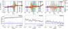 |
Fig. A.1 Bar pattern speeds of the three models under study from left to right, as measured using the TW method. Top panel: Pattern speed as a function of galactic longitude, the color of the curve indicating the time at which the measurement was made. At longitudes of 15 to 35 degrees, the TW method fails to give meaningful results because the assumption that only one pattern is rotating is not verified: this is where the bar and the spiral overlap. Two different pattern speeds are seen on the two sides of this interface region: the bar at lower longitudes, the spiral’s at higher longitudes. Bottom panel: Pattern speed of both the bar (black) and the spiral (blue) as a function of time, as averaged in the longitude ranges indicated in the top panel. Pattern speeds of the bar and the spiral both oscillate on the timescale of their beat frequency, and their coupling causes their pattern speed to anticorrelate, as shown by Hilmi et al. (2020). A linear regression of the pattern speeds is plotted as a dashed line, showing their global evolution. While the bars in Model2 and Model3 slow down, the bar in Model1 is speeding up. |
Appendix B Observational biases
In order to properly compare APOGEE DR17 data with the simulated galaxies, we biased the last snapshot of the models with APOGEE selection effects and uncertainties. This was only applied in section 4.2 when comparing the last snapshot of the models to the observations.
B.1 Selection effects
The two most important parameters of our analysis were radial positions and ages. Therefore, we tried to reproduce the radial distributions of monoage (1 Gyr wide) distributions seen in the APOGEE sample. The oldest stars not being very numerous, we grouped all stars older than 11 Gyr into one bin. The first step was to fit these distributions, histrogrammed in 0.5 kpc-wide bins, with a sum of 1, 2 or 3 Gaussians, each time choosing the model minimising the Corrected Akaike Information Criterion. This criterion allows to choose the simplest model (smallest amount of parameters) that best fits the data (smallest residual). The result of this first step is shown in Fig. B.1. The next step was to sample the simulations so that they had similar monoage radial distributions. To achieve this, we implemented a rejection sampling algorithm. Rejection sampling starts from a large original sample, and samples it to a more restricted target distribution. Here the original samples were the simulations’ monoage radial distributions, binned in 0.5 kpc-wide cells, while the target distributions were the selection functions fitted from the data (Fig. B.1). To avoid biases toward the most populated age bins, each age bin was given the same number of stars as counted in the APOGEE sample. For each monoage populations, the same rejection sampling procedure was applied as follows.
Randomly pick a star in the simulation.
Find the radial bin it belongs to.
Pick a random number below the total number of stars found in this radial bin. If this number is below the selection function calculated at the radius chosen, then the star is accepted. Otherwise, it is rejected.
Repeat until there are as many accepted stars as observed in the corresponding APOGEE bin.
The result of this procedure is shown for Model1 in Fig. B.2. We tried constraining the sample to azimuthal ranges consistent with the position of the Sun with respect to the bar in the Milky Way, but since the Galaxy is already well phase-mixed, this did not significantly impact our results. We therefore kept the azimuthally averaged method described above
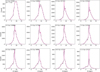 |
Fig. B.1 Radial distributions of different monoage bins in APOGEE DR17 sample. The pink curve is the best fit to the data. |
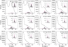 |
Fig. B.2 Final stars (filled gray) chosen from the total simulation (black line). They were selected so that each monoage populations of the sample are similarly radially distributed as in the APOGEE sample (pink lines). |
B.2 Uncertainties
We implemented Gaussian errors in the simulations for r, z, vr, vphi, vz, age and [Fe/H] with standard deviations reported in TableB.1 The errors on birth radius depending largely on age, we modeled their uncertainties on an age-by-age basis, similarly as when accounting for the selection effects. We fitted the distribution of APOGEE birth radius errors for monoage populations (1 Gyr wide with 1, 2 or 3 gaussians, keeping the model that minimized the Corrected Akaike Information Criterion. In Fig. B.3, histograms o the error distributions for different monoage bins of the APOGEE simple are shown as the black curves. The pink curves are the fitted models. We implemented these uncertainties using again a rejection sampling method. For each age bin, the original sample was artificially chosen as uniform between the minimal and maximal errors (ERb,min, ERb,max) observed in the corresponding APOGEE age bin. It is shown as the black curve in Fig. B.4 for Model1. In other words, each error between ERb,min and ERb,max originally has the same probability of being attributed to a star. We can then sample that error distribution to better represent the observed one Therefore, the same steps as indicated in section B.1 were applied, the original sample being histogrammed into 0.1 kpc-wide bins The filled gray histogram in Fig. B.4 shows the resulting error distribution sample.
Standard deviations of the Gaussian error distributions implemented in the simulations.
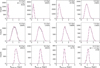 |
Fig. B.3 Birth radius error distributions of different monoage bins in the APOGEE DR17 sample. The pink curves are the best fit to the data. |
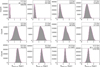 |
Fig. B.4 Modeled error on birth radius for different monoage bins in Model1. The black curve is a default arbitrary uniform distribution of errors. The pink curve is the APOGEE birth radii error distributions. The filled gray histogram is the error distribution drawn from the uniform distribution (black) so that it fits the data (pink). |
Appendix C Migration over longer time intervals
A usual way to visualize radial migration in simulations is by plotting the change in guiding radius between two snapshots as a function of the initial guiding radius. Changing the time separation between these two snapshots will affect the appearance of these plots. When choosing the right times and the right time interval, the variations in the amplitude of the ridge at bar radius appears just as in Fig. 2. However, if the times are not chosen at bar and spiral connection and disconnection and/or if the time interval is too large, these variations caused by the regular bar-spiral overlap will be diluted, as other mechanisms will enter into play and create ridges at other positions. Figure C.1 shows ∆Rg as a function of R0 for a time interval of ∆t = 0.5 Gyr (as opposed to ∆t = 0.1 Gyr for Fig. 2). As for Fig. 2, each row is for a different model, while each column is for a different time in the evolution of the galaxies. The plane is divided into 0.3x3.3 kpc2 bins for Model1 and Model2, and 0.3x4.7 kpc2 bins for Model3 and the number of stars in those bins is given by the color bar, with contribution only from stars present throughout the whole period. Strong ridges are seen in all models near the bar CR, while the ridges at the bar radius are much less pronounced because of the large time interval used here. For Model3 (last row), the amplitude of the ridge decreases with time. This most likely results from the disk getting hotter, both numerically and due to the absence of cold gas accretion (in an isolated context), and thus less sensitive to perturbations.
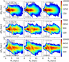 |
Fig. C.1 2D-histograms of the change in guiding radius ∆Rg between two snapshots separated by ∆t = 0.5 Gyr, with respect to the initial guiding radius R0. From top to bottom, each row represents stars from Model1, Model2 and Model3. Each column represents a different time in the galaxies’ evolution, increasing from left to right. These times are taken randomly, and the time interval is bigger than that used in section 4. The solid black and pink lines indicate respectively the bar radius and the CR. Strong ridges near these two radii are present in all models. However, the varying amplitude seen in Fig. 2 are not visible here. Model3 shows decreasing ridge amplitude, most likely as a sign of the galaxy getting hotter with time through numerical heating and absence of cold gas accretion (so less sensitive to perturbations). |
All Tables
Standard deviations of the Gaussian error distributions implemented in the simulations.
All Figures
|
Fig. 1 Face-on (top row) and edge-on (bottom row) density map of the three models (from left to right) at the last snapshots, and the APOGEE DR17 sample used (right). The dashed black circle indicates the bar length, while the pink circle indicates the bar CR. They coincide for Model1. The black star indicates the location of the (simulated) Sun. Rotation is in the counterclockwise direction. The 2 × 2 kpc2 squares show the regions that will be studied in Figs. 4, 5, 8, and 10. Light blue indicates the left side of the bar, while orange indicates the right side of the bar. The solid squares are on the trailing side of the bar, while the dashed squares are on the leading side of the bar, although leading and trailing sides will not be differentiated in Sect. 5 (only one 2 × 2-kpc2 square per edge). The black and gray color indicates squares along the bar minor axis. These two squares will be stacked together and averaged in Sect. 4. |
| In the text | |
|
Fig. 2 Change of guiding radius over ∆t = 0.1 Gyr vs. initial guiding radius for Modell, Model2, and Model3 stars from top to bottom. Each column represents a different initial time, which increases from left to right as indicated in the top of each panel. These times were chosen to be at moments when the bar and the spiral are connected or disconnected. The dashed horizontal black line shows ∆Rg = 0, (i.e., no migration). All points above (below) this line represent stars that migrated outward (inward). The solid black line indicates the bar length, while the pink line indicates the bar corotation radius. They coincide for Model1. The vertical dashed lines in the bottom panel indicate the radial range over which the azimuthal variations of migration are investigated in Fig. 3. Panels corresponding to bar-spiral connection times show a very prominent ridge at the bar end, while this ridge is much less pronounced at bar-spiral disconnection times, except for Model1 where the weak spirals diminish this effect. |
| In the text | |
|
Fig. 3 Two-dimensional histograms of the change in guiding radius over ∆t = 0.1 Gyr with respect to the initial azimuthal angle for stars in Model3 initially in different 2-kpc-wide radial bins. Each column is for a different radial bin, going further out from left to right as indicated in each panel. The bar ends (Rbar = 3.15 kpc) are encompassed in the second column and are indicated by the bold text, while the corotation (RCR = 5.3 kpc) is at the border of the fourth and fifth bins and is indicated in pink. The left and right sides of the bar are shown by the light blue and orange vertical dotted lines, respectively. The solid lines indicate the trailing side of the bar edges, while the dashed lines indicate their leading sides. Those lines are located at the edge of their associated square regions from Fig. 1. The different rows represent the same quantities at different times in the disk evolution. They are the same times as those in the first two columns of Fig. 2, and thus show a time at which the bar is connected to a spiral (first row), as well as a time when the bar is not connected to any spiral (second row). The (φ-∆Rg) plane of Fig. 3 is divided into 5° × 0.1 kpc bins and the number of stars in those bins is given by the color bar, with a contribution only from stars present throughout the whole period. The full temporal evolution over the last 1.4 Gyr of evolution is available as an online movie. |
| In the text | |
|
Fig. 4 Time evolution of migration strength from different galactic disk radii in Model3. In each panel, the different curves correspond to the migration strength (i.e., how far stars found in this region at some time, t, migrate after ∆t) of stars originally found in each of the squares shown in Fig. 1. Light blue and orange indicate the left and right sides of the bar, respectively, while solid and dashed represent the trailing and leading sides of the bar, respectively. The gray curve is the mean migration strength along the bar minor axis (i.e., the two gray squares of Fig. 1). From left to right, these squares are shifted horizontally (light blue and orange) and vertically (gray), along the bar major and minor axis, respectively, to probe different radii. |
| In the text | |
|
Fig. 5 Time evolution of different migration statistics compared to bar length time evolution, for the three models (from left to right). Different azimuths around the bar radius are scanned using the six 2 × 2 kpc2 square regions shown in Fig. 1. The gray curve is the mean statistical quantity over the two squares placed along the bar minor axis. Again, blue and orange curves represent the left and right sides of the bar, respectively, while solid and dashed lines stand for the leading and trailing sides of the bar, respectively. The number of peaks of these curves is indicated as N̄peaks in the top and bottom panel; N̄peaks is the mean Npeaks over the different curves. First row: standard deviation of the change in guiding radius over ∆t = 100 Myr experienced by all stars located in the six different square-shaped regions. Second row: same as top row, but for the mean change in guiding radius, which slows the net angular momentum transfer. Third row: mean guiding radius after ∆t = 100 Myr for the 5% stars that migrate the most. Last row: time evolution of the bar half-length. The peaks correspond to moments when the bar is connected to a spiral arm. The maxima in the migration strength, or their frequency, coincide with those of the bar half-length, which indicates that they are a result of the interaction between the bar and spiral arms. |
| In the text | |
|
Fig. 6 Birth radius distribution of stars found at the solar radius today (inside the gray vertical strip) of, from left to right, the two cosmological models Model1 and Model2, and the APOGEE DR17 red giant sample. The black curves are for the whole sample. In the top row, the blue and yellow curves highlight stars found today on orbits with e < 0.2 (cold) and 0.2 ≤ e < 0.5 (warm), respectively. The percentages that warm and cold stars born inside Rbar represent in the SNd are indicated in the top right of the panels for each galaxy. In the middle row, Rbirth distributions are shown for different monoage populations. From purple to red, stars get older and older, as indicated in the color bar. In the bottom row, Rbirth distributions are shown for different metallicity bins, blue and red representing metal-poor and metal-rich stars, respectively as indicated in the color bar. |
| In the text | |
|
Fig. 7 Age distribution of stars found at solar radius today but born inside Rbar. The two curves follow the same line style and color code as in the top row of Fig. 6: solid for stars born inside Rbar, blue and yellow for kinematically cold and warm stars, respectively. The percentages in the legend are the proportion each eccentricity population with Rbirth < Rbar represents in the whole solar radius sample indicated in gray in Fig. 6. In the three cases, both the cold and warm distributions are mostly old (10 Gyr in the models, 8–9 Gyr in the data) with a tail to younger ages. |
| In the text | |
|
Fig. 8 Modell star formation temporal evolution in 2 × 2 kpc2 square regions centered at increasing radii from left to right and top to bottom, spanning radii from 2.25 kpc to 5.25 kpc. The squares of the leading and trailing sides of the bar, shown in Fig. 1, are merged into one square per edge of the bar centered on (x, y) = (±R, 0), light blue and orange indicating the left and right side, respectively. The upper and lower edges of the bar minor axis are differentiated, using black and gray, respectively. The regions at the bar ends show i) lots of fluctuations, ii) more star formation than along the bar minor axis until just outside the bar radius. |
| In the text | |
|
Fig. 9 Mass of gas (top panel) and star formation efficiency (bottom panel) across time in Model1 and Model2 from left to right, for the four regions used in Figs. 8 and 10. There is slightly less gas along the minor axis of the bar compared to its major axis, which partially explains the lower number of newly born stars in the former. However, the main reason for the higher number of newly born stars at the bar major axis is the much higher SFE, as seen in the bottom panel. The time evolution of SFE at the two sides of the bar (blue and orange) often anticorrelates, which suggests the presence of a nonbisymmetric spiral structure. |
| In the text | |
|
Fig. 10 Comparison of the time evolution of the star formation in the four square regions used in Fig. 8 (top row) to that of the bar half-length (bottom row), for Model1 and Model2 (left and right column, respectively). Peaks in Rbar correspond to the times of bar-spiral connection. The frequency of these bar length peaks coincides with the frequency of the starbursts seen in the top panel (see number of peaks Npeaks in each panel), which suggests their correlation with the periodic bar-spiral overlaps. Starbursts do not always happen at the same time at the two ends of the bar. |
| In the text | |
|
Fig. 11 Distribution of HII regions in the Milky Way as a function of galactic longitude. The red curve is a kernel density estimate of the histogram, in black, which shows data from the WISE catalog. Regions shaded in blue and orange are in the direction of the near and far side of the bar, respectively. There are twice as many objects in the direction of the near end of the bar compared to that of the far end of the bar. |
| In the text | |
|
Fig. A.1 Bar pattern speeds of the three models under study from left to right, as measured using the TW method. Top panel: Pattern speed as a function of galactic longitude, the color of the curve indicating the time at which the measurement was made. At longitudes of 15 to 35 degrees, the TW method fails to give meaningful results because the assumption that only one pattern is rotating is not verified: this is where the bar and the spiral overlap. Two different pattern speeds are seen on the two sides of this interface region: the bar at lower longitudes, the spiral’s at higher longitudes. Bottom panel: Pattern speed of both the bar (black) and the spiral (blue) as a function of time, as averaged in the longitude ranges indicated in the top panel. Pattern speeds of the bar and the spiral both oscillate on the timescale of their beat frequency, and their coupling causes their pattern speed to anticorrelate, as shown by Hilmi et al. (2020). A linear regression of the pattern speeds is plotted as a dashed line, showing their global evolution. While the bars in Model2 and Model3 slow down, the bar in Model1 is speeding up. |
| In the text | |
|
Fig. B.1 Radial distributions of different monoage bins in APOGEE DR17 sample. The pink curve is the best fit to the data. |
| In the text | |
|
Fig. B.2 Final stars (filled gray) chosen from the total simulation (black line). They were selected so that each monoage populations of the sample are similarly radially distributed as in the APOGEE sample (pink lines). |
| In the text | |
|
Fig. B.3 Birth radius error distributions of different monoage bins in the APOGEE DR17 sample. The pink curves are the best fit to the data. |
| In the text | |
|
Fig. B.4 Modeled error on birth radius for different monoage bins in Model1. The black curve is a default arbitrary uniform distribution of errors. The pink curve is the APOGEE birth radii error distributions. The filled gray histogram is the error distribution drawn from the uniform distribution (black) so that it fits the data (pink). |
| In the text | |
|
Fig. C.1 2D-histograms of the change in guiding radius ∆Rg between two snapshots separated by ∆t = 0.5 Gyr, with respect to the initial guiding radius R0. From top to bottom, each row represents stars from Model1, Model2 and Model3. Each column represents a different time in the galaxies’ evolution, increasing from left to right. These times are taken randomly, and the time interval is bigger than that used in section 4. The solid black and pink lines indicate respectively the bar radius and the CR. Strong ridges near these two radii are present in all models. However, the varying amplitude seen in Fig. 2 are not visible here. Model3 shows decreasing ridge amplitude, most likely as a sign of the galaxy getting hotter with time through numerical heating and absence of cold gas accretion (so less sensitive to perturbations). |
| In the text | |
Current usage metrics show cumulative count of Article Views (full-text article views including HTML views, PDF and ePub downloads, according to the available data) and Abstracts Views on Vision4Press platform.
Data correspond to usage on the plateform after 2015. The current usage metrics is available 48-96 hours after online publication and is updated daily on week days.
Initial download of the metrics may take a while.