| Issue |
A&A
Volume 701, September 2025
|
|
|---|---|---|
| Article Number | A148 | |
| Number of page(s) | 27 | |
| Section | Interstellar and circumstellar matter | |
| DOI | https://doi.org/10.1051/0004-6361/202555085 | |
| Published online | 10 September 2025 | |
Observations of carbon radio recombination lines with the NenuFAR telescope
I. Cassiopeia A and Cygnus A
1
Laboratoire de Physique de l’École Normale Supérieure, ENS, Université PSL, CNRS, Sorbonne Université, Université Paris Cité,
75005
Paris,
France
2
LUX, Observatoire de Paris, Université PSL, Sorbonne Université,
75014
Paris,
France
3
Institute of Radio Astronomy NAS of Ukraine,
4, Mystetstv St.,
Kharkiv
61002,
Ukraine
4
LIRA, Observatoire de Paris, Université PSL, Sorbonne Université,
75014
Paris,
France
5
Green Bank Observatory, Green Bank,
WV
24944,
USA
6
Université de Strasbourg, CNRS, Observatoire Astronomique de Strasbourg,
UMR 7550,
67000
Strasbourg,
France
7
INAF – Osservatorio Astrofisico di Arcetri,
Largo E. Fermi 5,
50125
Firenze,
Italy
8
Université Paris Cité and Université Paris Saclay, CEA, CNRS, AIM,
91190
Gif-sur-Yvette,
France
9
Instituto de Física Fundamental (CSIC),
Calle Serrano 121-123,
28006
Madrid,
Spain
10
LPC2E, OSUC, Univ. Orléans, CNRS, CNES, Observatoire de Paris, Université PSL,
45071
Orléans,
France
11
ORN, Observatoire de Paris, Université PSL, Université d’Orléans, CNRS,
18330
Nançay,
France
12
Department of Physics and Astronomy, The University of Western Ontario,
1151 Richmond Street,
London,
Ontario
N6A 3K7,
Canada
13
Research School of Astronomy & Astrophysics, Australian National University,
Canberra,
ACT
2610,
Australia
14
Laboratoire Univers et Particules de Montpellier (LUPM) Université Montpellier,
CNRS/IN2P3, CC72, place Eugène Bataillon,
F-34095
Montpellier Cedex 5,
France
15
Kapteyn Astronomical Institute, University of Groningen,
PO Box 800,
9700 AV
Groningen,
The Netherlands
16
Université Grenoble Alpes, CNRS, IPAG,
38000
Grenoble,
France
17
Leiden Observatory, Leiden University,
Leiden,
The Netherlands
★ Corresponding author: This email address is being protected from spambots. You need JavaScript enabled to view it.
Received:
8
April
2025
Accepted:
21
July
2025
Abstract
Context. Carbon radio recombination lines (CRRLs) at decametre wavelengths trace the diffuse phase of the interstellar medium (ISM) of the Galaxy. Observations of these lines allow for physical parameters of this phase to be measured.
Aims. We observed CRRLs with the recently commissioned New Extension in Nançay Upgrading LOFAR (NenuFAR) telescope towards two of the brightest sources at low-frequency (10–85 MHz): Cassiopeia A and Cygnus A (hereafter, Cas A and Cyg A, respectively). We then measured the density, ne, and temperature, Te, of the electrons in line-of-sight clouds.
Methods. We used NenuFAR’s beam-forming mode and integrated several tens of hours on each source. The nominal spectral resolution was 95.4 Hz. We developed a reduction pipeline primarily aimed at removing the radio frequency interference (RFI) contamination and correcting the baselines. We then performed a first fitting of the spectral lines observed in absorption associated with the line-of-sight clouds.
Results. Cas A is the brightest source in the sky at low frequencies and represents an appropriate test bench for this new telescope. On this source, we detected 398 Cα lines between the principal quantum numbers n = 426 and n = 826. Cyg A is also a bright source, however, the Cα lines were observed to be fainter. We stacked the signal by groups of a few tens of lines to improve the quality of our fitting process. For both sources, we reached a significantly higher signal-to-noise ratio (S/N) and spectral resolution than the most recent detections by the LOw Frequency ARray (LOFAR). The variation of the spectral line widths with the electronic quantum number provides constraints on the physical properties of the clouds: Te, ne, and the temperature, T0, of the radiation field, the mean turbulent velocity, νt, and the typical size of the cloud.
Conclusions. Our final constraints differ from those inferred from LOFAR results, with ∼50% lower Te, ∼35% lower ne, and from 10 to 80% higher νt, on average. The NenuFAR observations sample a larger space volume than LOFAR’s towards the same sources due to the differences in instrumental beam sizes. These discrepancies highlight the sensitivity of low-frequency CRRLs as probes of the diffuse ISM, paving the way towards large area surveys of CRRLs in our Galaxy.
Key words: line: profiles / ISM: clouds / ISM: structure / radio lines: ISM / ISM: individual objects: Cassiopeia A / ISM: individual objects: Cygnus A
© The Authors 2025
 Open Access article, published by EDP Sciences, under the terms of the Creative Commons Attribution License (https://creativecommons.org/licenses/by/4.0), which permits unrestricted use, distribution, and reproduction in any medium, provided the original work is properly cited.
This article is published in open access under the Subscribe to Open model. This email address is being protected from spambots. You need JavaScript enabled to view it. to support open access publication.
1 Introduction
Our understanding of the life cycle of interstellar matter from molecular clouds to ionised phases and encompassing star formation is incomplete. Two key questions in the context of radio recombination lines (RRLs) and the diffuse interstellar medium (ISM) are related to (i) the processes of radiative and mechanical feedbacks exerted by young massive stars on their neutral interstellar environment and (ii) the ability of the neutral interstellar gas to return to a molecular phase. Studies of both aspects will benefit from the determination of the ionisation fraction or, equivalently, the fractional abundance of free electrons. Indeed, although it is neutral in the sense that its main constituents (H and He) are in neutral forms, the neutral ISM can maintain a small ionisation fraction (from ∼10−8 in its densest, molecular phases to∼10−1 in the warm neutral medium). Several processes contribute to this ionisation. Stellar FUV photons (with energies between 6 eV and 13.6 eV, the latter value being the ionisation potential of hydrogen) can penetrate into neutral gas and ionise carbon and sulphur atoms (respectively of 11.26 and 10.36 eV ionisation potential). This is the case in photodissociation regions (PDRs) and, more precisely, in the unshielded surface layer of dense molecular clouds directly illuminated by nearby young massive stars (e.g. Joblin et al. 2018; Peeters et al. 2024 and references therein). This is also the case more generally in the diffuse interstellar gas, widely permeated by the ambient Galactic stellar UV radiation(Heays et al. 2017). Dynamical processes such as shocks can also partially ionise the gas (e.g.Godard et al. 2024), whereas cosmic rays are the only possible source of ionisation in the densest parts of molecular clouds(Dalgarno 2006; Padovani et al. 2009; Padovani et al. 2018). Measuring the ionisation fraction in the ISM is paramount since beyond playing a key role in its chemistry, it controls its heating (e.g. through the photoelectric effect on interstellar dust grains), cooling (e.g. through the excitation of key species), and the excitation of key species (e.g. common molecular tracers with high dipole moments such as HCN and HCO+). Until recently, measuring the ionisation fraction had systematically been done by modelling the line emission from carefully selected species with astrochemical models (see e.g. Bron et al. 2021, for a review).
Over the past 20 years, instrumental progress has resulted in the development of a new strategy to observationally constrain this parameter in the neutral interstellar regions, based on the observation of recombination lines, in particular, from carbon, across various frequency ranges. Indeed, in presence of UV radiation, carbon is the main electron provider in these regions. Carbon atoms undergo a rapid cycle of ionisation followed by recombination with the free electrons present in the gas. During these recombinations, the species recombine in very excited electronic states and then cascade to lower energy states, emitting a large number of recombination lines. The shape of these recombination lines depends on the physical conditions (in particular, the electron density and electron temperature), where the recombination occurs. Therefore, they constitute a probe of the ionisation fraction and physical properties of the diffuse ISM.
A review of recent RRLs observations. In recent years, lines have been observed in the low frequency radio range (<1 GHz) in absorption against bright Galactic radiosources; namely, carbon radio recombination lines (CRRLs). For instance, Stepkin et al. (2007) observed series of carbon α, β, γ, and δ recombination lines (hereafter, ‘Cα’, ‘Cβ’, ‘Cγ’, and ‘Cδ’) in absorption towards Cassiopeia A (hereafter, Cas A). These lines arose, respectively, from the principal quantum numbern + 1,n + 2,n + 3,n + 4 → n de-excitations with the UTR-2Ukrainian radiotelescope around 26 MHz. Their detections of Cδ lines with n ∈ [625, 1005] enabled the estimation of the electron temperature and density in line-of-sight clouds by fitting the evolution of the line width with the quantum number of the upper level of the transition. After Asgekar et al. (2013) proved the feasibility of using LOFAR to study low-frequency C518α to C548α RRLs towards sources such as Cas A, Oonk et al. (2017) complemented this study of line-of-sight clouds towards this source with LOFAR observations in the 33–78 MHz and 304–386 MHz ranges. They detected series of hydrogen and carbon recombination lines in emission and absorption in three line-of-sight clouds, which led them to obtain better constrained measurements of the electron density, ne, and temperature,Te, to pinpoint the origin of the CRRLs in the CO-dark surface layers of molecular clouds, where most of the carbon is ionised but the hydrogen is already molecular, and to estimate lower limits to the cosmic-ray ionisation rate. Simultaneously, Salas et al. (2017) combined lower frequency (10–33 MHz) observations of CRRLs with observations of the 158 µm [CII] line to yield estimates of ne and Te in the same clouds. The values they found were consistent with those of Oonk et al. (2017) and Stepkin et al. (2007). Finally, for this source, Salas et al. (2018) and Chowdhury & Chengalur (2019) mapped CRRLs with, respectively, LOFAR (at 43, 54, 148 and 340 MHz) and the GMRT (in the 410– 450 MHz range). Their comparisons with other tracers of the ISM(HI, OH, CO, CI, CII...) confirmed the utility of CRRLs as tracers of diffuse HI and CO-dark gas halo’s around molecular clouds. The second brightest source in the low-frequency range, Cygnus A (hereafter Cyg A), was also observed with LOFAR byOonk et al. (2014) to detect CRRLs. This study also constrained the electron density and temperature in one Galactic line-of-sight component. The smaller number of detected components could be explained by the higher Galactic latitude of the background source, b = + 5.76°, compared to b = −2.13° for Cas A. The modelling framework for extracting measurements of the physical parameters from these Galactic observations of CRRLs (i.e. the level population problem of recombining carbon ions) was updated by Salgado et al. (2017a,b). These authors calculated departure coefficients in the hydrogenic approximation including low-temperature dielectronic capture effects, providing a study of CRRLs emission and absorption in a range of conditions in the diffuse, cold neutral medium (CNM).
Beyond our Galaxy, a handful of studies report detections of RRLs in the low-frequency regime (below ~1 GHz). First,Morabito et al. (2014) discovered CRRLs in absorption in the M82 galaxy with a 8.5 sigma detection obtained by stacking 22 alpha transitions with n = 468–508 with the LOFAR telescope, although this result was only replicated with a lower signal-to-noise ratio (S/N) by Emig et al. (2020). They found that these lines were likely to be associated with cold atomic gas in the direction of the nucleus of M82, but their detection was not sufficient to measure physical parameters associated with the local medium. This shortcoming was remedied towards the 3C190 radio quasar at z ~ 1.1946 by Emig et al. (2019) with LOFAR observations. They demonstrated that H and/or C RRLs can be used to infer constraints on electron temperature and density in a line-of-sight dwarf galaxy about 80 Mpc from 3C190.Emig et al. (2023) then reported the detection of hydrogen RRLs with the MeerKAT telescope around 1 GHz, from a z ~ 0.89-galaxy that intercepts and lenses the PKS 1830-211 blazar. They were able to tie their detections to hydrogen and to use them to measure the star formation rate within the lensing galaxy. Generally speaking, new perspectives in various directions are arising from recent RRL observations, in relation to observations of multi-ionised species(Liu et al. 2023), heavier species than H, He, and C (e.g. sulphur, see Goicoechea & Cuadrado 2021) and thanks to the development of new reduction and interpretation techniques(Emig et al. 2020).
In the present study, we focus on the observation of Cα recombination lines with the newly commissioned New Extension in Nançay Upgrading LOFAR (NenuFAR) telescope towards the two brightest low-frequency radio sources: Cassiopeia A and Cygnus A, between 10 and 85 MHz. At these frequencies, CRRLs are detected in absorption in foreground interstellar clouds. In Sect. 2, we briefly review the sources and the existing observations in similar ranges, and we present the NenuFAR instrument. In Sect. 3, we present the reduction pipeline developed to recover up to 90% of the 443 transitions within the frequency range. In Sect. 4, we present our fitting of the observed lines, highlighting our determinations of physical parameters, such as the electron density and electron temperature. In Sect. 5, we compare our results to equivalent observations when possible. Sect. 6 presents our concluding remarks.
2 Experimental setup
2.1 The NenuFAR telescope
The New Extension in Nançay Upgrading LOFAR (NenuFAR,Zarka et al. 2020) telescope is located at the Nançay Radioastronomy Observatory. NenuFAR is a low-frequency radio phased array and interferometer. We used it as a standalone phased array, although it will also be used as an extension of LOFAR. Nenu-FAR was designed as a pathfinder to the Square Kilometre Array (SKA1). Its elementary receiving antennas consist of crossed inverted V-shaped dual-polarisation dipoles. The antennas are organised in hexagonal tiles called mini-arrays (MA) that comprise 19 such antennas apiece. The MA beam of the hexagonal MA is analogically steerable across various directions in the sky. Due to the hexagonal symmetry, grating lobes are present in the individual MA primary beam(Girard & Zarka 2023). To mitigate this, the MAs are rotated relative to each other by angles in multiples of 10 degrees, implying six non-redundant orientations. At present, NenuFAR is built at 85% and features 80 MAs in its core2. Figure 1 illustrates the NenuFAR configura-tion3. The large dense core provides a high sensitivity, making it particularly effective for detecting faint low-frequency RRLs. All MAs are analogue phased using delay lines, and the entire array is digitally pointed quasi-continuously (at 10 s steps) towards the target.
Operating within the frequency range from the Earth’s ionospheric cut-off at −10 MHz to the radio FM band at ~85 MHz, NenuFAR’s core provides varying angular resolution from 3.59° to 25′ for 80 MAs. The two linear polarisations outputs of each MA (NE-SW and NW-SE) are connected in parallel to multiple receivers, enabling operation in four distinct modes: standalone beam-former, standalone imager, waveform capture mode, and an upgraded LOFAR station mode that combines NenuFAR with the International LOFAR Telescope through the Nançay LOFAR station (FR606) is also shceduled. NenuFAR’s main LOFAR-like Advanced New Backend (LANewBa) provides fluxes of complex waveform time series within 195.3125 kHz wide beamlets at a time resolution of 5.12 μs. This flux can be numerically channelised down to δ f ≃ 95 Hz at the expense of a lower time resolution of dt ≃ 10 ms. The sensitivity of NenuFAR presently ranges from −50 mJy at 15 MHz to −15 mJy at 85 MHz for a one-hour integration time with a frequency bandwidth of ∆ f = 10 MHz. At the nominal spectral resolution of 95.4 Hz, and for an on-source time of 2 h, the instrument achieves a sensitivity of -9 Jy at 15 MHz and -3 Jy at 85 MHz. These characteristics make NenuFAR one of the most sensitive radio telescopes operating below 85 MHz(Zarka et al. 2020).
We used the NenuFAR telescope in beamforming mode, thanks to its Unified Dynamic Spectrum Pulsar and Time Domain (UnDySPuTeD) receiver. It is fed by the main backend LANewBa, which is itself fed by the number of operating mini-arrays ×2 polarisations (NE and NW) in the core. Our observations began in 2019 and were performed within the Early Science Project 10 (ES10) of NenuFAR, which was converted into a so-called long term (LT) program, LT10 at the end of 2021. During the ES10 phase, 56 mini-arrays were operational, later evolving to 80 in the LT phase. LANewBa digitises each of the {56 to 80} ×two input signals at a sampling frequency of 200 MHz. The data streams are then channelised in sub-bands of 200 MHz/1024 = 195.3125 kHz bandwidth each. Beamforming then consists in coherently summing up the complex data streams from all operating MAs for a given sub-band, polarisation, and direction (θ,φ) in the sky, after applying adequate phase shifts. A beamlet consists of one sub-band × two polarisations beamformed to one direction in the sky, meaning it is defined by a triplet (υc,θ,φ) with υc the central frequency of the sub-band. The raw data stream corresponding to one beam-let is the complex filtered waveform, that consists (on average) of 195312.5 pairs of complex X and Y signals values per second. LANewBa can compute and deliver 768 such beamlets at any given time, that correspond to an instantaneous usable bandwidth of 150 MHz. These 768 beamlets can be distributed in (υc,θ,φ) as desired, for instance over two pointed directions simultaneously observed (θ0, φ0) and (θ1, φ1) with 75 MHz bandwidth (i.e., the full band of the instrument) to 768 beams paving the analogue beam at a a single frequency, υ c, through any intermediate configuration. In the rather exploratory phase of our program that we describe here, we used a configuration aimed at acquiring the full available bandwidth in only one direction of the sky at a given time, thereby producing ‘only’ 384 beamlets.
The beamformed raw data from LANewBa were subsequently distributed via virtual local area network to several calculators, and especially to the two identical CPU/GPU ‘UnDyS-PuTeD’ calculators, that further channelise the beamlet data down to 95 Hz resolution (2048 channels per beamlet), compute the four Stokes parameters from the X and Y data, and perform time integration. Our observing setup consisted in using 384 beamlets over the 10.156–84.961 MHz frequency range, totaling 786 432 frequency channels with a resolution of −95.4 Hz. We set the time resolution to 84 ms with a Hamming-window apodisation. In this mode, the full width at half maximum (FWHM) of the observing beam was between 25.3′ (at −85 MHz) and 3.59° (at −10 MHz). The product of UnDySPuTeD is labelled as ‘level 0’ (L0) data. At this stage, the 384 beamlets were grouped in two ‘lanes’, labelled 0 and 1. Lane 0 contains the first half of the spectra (from 10 to about 47 MHz) and the lane 1 contains the second half of the spectra (from 47 to 85 MHz). The L0 data have a volume of the order of 260 GB/h/lane.
These data were subsequently reduced using an IDL software developed by Philippe Zarka and the NenuFAR team called read_nu_spec software, which aims to read, pre-process, reduce, and write level 1 (L1) data that have a volume reduced by a factor∼100, stored in FITS format. This first reduction step performs a first pass of radio-frequency interference (RFI) mitigation, correction or whitening of bandpass and gain, and integration of the spectrum from the nominal 84 ms time resolution to a final resolution of 30 s. The ‘L1 data’ output of read_nu_spec consists of a time-frequency table of Stokes I values and a table containing statistical weights for each timefrequency integrated pixel determined by the percentage of data not flagged in the original time-frequency interval corresponding to that pixel. The time-frequency tables are subdivided in two subtables corresponding to the two ‘lanes’ of equal frequency width containing each 192 sub-bands of 2048 frequency channels each. These level 1 data are the input of our reduction pipeline (see Fig. 2).
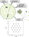 |
Fig. 1 Configuration of the NenuFAR telescope. Top panel: layout of all 96 mini-arrays forming the NenuFAR interferometer. Bottom panel: schematic layout of a mini-array showing the 19 inverted-V shape dual polarisations antennas. They are arranged in a 5.5 m triangular lattice forming a hexagon (from Girard & Zarka 2023). |
2.2 Observed sources
We selected two radio sources to perform our experiment: Cassiopeia A and Cygnus A. They are the two brightest radio sources in the observed frequency range(de Gasperin et al. 2020) and they were previously observed by LOFAR LBA(Oonk et al. 2014, 2017; Salas et al. 2017). Hence, they optimise the chances of success of an absorption experiment, and represent an interesting benchmark for our new method of analysis using NenuFAR. The LOFAR observations of Cassiopeia A and Cygnus A were performed in imaging mode and then the maps were cropped at the angular extension of the radio sources. Cassiopeia A (Cas A) is a supernova remnant (SNR) and the brightest radio source in the northern sky, with 27 104 Jy at 50 MHz(de Gasperin et al. 2020). CO(Zhou et al. 2018) and RRLs(Oonk et al. 2017; Salas et al. 2017) observations revealed different velocity components along the line of sight in foreground clouds in the Perseus arm and the Orion spur. These clouds are detected at three different velocities: –47, –38 and 0 km s−1. Cygnus A (Cyg A) is a radio galaxy, and the second brightest radio source in the northern sky, with 22 146 Jy at 50 MHz(de Gasperin et al. 2020). In the foreground of Cygnus A, HI-21 cm(Mebold & Hills 1975) and CRRLs(Oonk et al. 2014) indicat the presence of CNM at∼3.5 km s−1 in the Orion spur. Table 1 provides the main characteristics and observation time of the sources. The largest angular size at 50 MHz of Cas A and Cyg A are 7.4′ and 2.3′, respectively. Therefore, it is clear that the beam of NenuFAR always encompasses the source.
3 Analysis pipeline
From L1 data level, the analysis pipeline is divided in two major steps: a processing step aiming at providing a scientifically usable data product per observing block and per frequency channel, described in Sect. 3.1, and a post-processing step consisting in a time integration and line stacking, described in Sects. 3.2 and 3.3.
3.1 L1 data processing
The goal of the processing step is to remove RFI and flatten the continuum baseline to produce one optical depth spectrum covering the whole 10–85 MHz range per observing block. These goals were progressively achieved via: (a) a first, large-scale, lane-by-lane correction described in Sect. 3.1.1; (b) a finer correction at sub-band scale described in Sect. 3.1.2; and (c) the concatenation of all 384 sub-bands with a final mitigation over the whole spectrum described in Sect. 3.1.3. A functional diagram is presented in Fig. 2. In the following, each step of the process is illustrated on the example of a two-hours observing block acquired on the 20/09/2021 between 1 a.m. and 3 a.m. towards Cassiopeia A (see Figs. 3, 4, and 5).
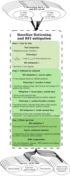 |
Fig. 2 Functional diagram for the processing of L1 level data (see Sect. 3.1). The algorithm is split in three reduction layers: lane-by-lane (top, 2a, Sect. 3.1.1), sub-band-by-sub-band (middle part, 2b, Sect. 3.1.2) and whole spectrum (bottom, 2c, Sect. 3.1.3). The processing consists of an iterative series of RFI mitigation and baseline flattening steps, followed by its application to real data illustrated in Fig. 3. |
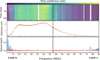 |
Fig. 3 Description of the step 1 of the data processing algorithm (see top part of Fig. 2). The top panel represents the time-frequency table, I(nt, nυ), issued by the pre-processing algorithm read_nu_spec. Middle panel shows the spectrum integrated over the two hours of observations, in arbitrary units. Bottom panel shows the flattened spectrum before (blue) and after (red) 3 rms clipping. |
Characteristics of the radio sources.
3.1.1 Lane by lane
We first integrated the Stokes I time-frequency L1 tables over the time axis weighted by the statistical weights determined by read_nu_spec, in order to obtain a single spectrum integrated over two hours (see top panels of Fig. 2 for the functional diagram and those of Fig. 3 for the data illustration). The integrated spectrum, denoted I, shows variability on multiple scales: a wide broadband variability over the whole frequency range (see middle panel of Fig. 3) and a smaller narrowband variability at sub-band scale. To correct the wide variability, we empirically determined the global shape of the integrated spectrum by rebinning it to 192 points (one per sub-band) per lane. With a linear interpolation of the rebinned spectrum, we defined Ismooth(υ), and computed the optical depth,  , at the nominal spectral resolution of our data. The linear approximation is sufficient at this stage, and potential deformations are dealt with in a subsequent step. Finally we applied a 3 rms clipping on τ(υ) to remove the RFI, where rms is the root mean square of the spectrum. The rms is evaluated in a sliding window over the whole flattened lane. The size of the window is 2048 channels, which is the size of a sub-band. The bottom panel of Fig. 3 shows the optical depth spectrum before and after the clipping.
3.1.2 Sub-band by sub-band
The next step consists in correcting for the narrowband variability and mitigating the RFI at subband scale. Indeed, the sub-band data from the NenuFAR beamformer generally presents an ‘S-shape’ distortion, because of which some RFI have escaped the mitigation at lane scale. The various steps of the reduction applied to one subband are described in Fig. 2 and an illustration can be found in Fig. 4. We first mitigated RFI by targeting potential narrow spikes (over a few frequency channels) within each sub-band. To this aim, we performed a 3 rms clipping on the gradient of the subband where anomalous spikes can be identified and removed. This step is labelled as ‘RFI mitigation 2″ in Fig. 2, and panel a of Fig. 4 shows the sub-band before and after the operation.
We then approximated the S-shape distortion of each sub-band by the median of 11 successive sub-bands (±5 sub-bands around the considered one, or + k/ - (10 - k) if the sub-band is near the edges of the spectrum), median which is then smoothed with a Savitzky-Golay filter. In some cases, we had to discard anomalous sub-bands that presented a general shape that differed significantly from its neighbours. This operation is described in Appendix A. In order to preserve potential signal throughout all these operations, we applied a mask around the frequency of expected lines. The width of the mask around each predicted line has been determined empirically and depends on the source, but is typically∼5.7 kHz (∼60 frequency channels), that is 27 km s−1 at 85 MHz and 172 km s−1 at 10 MHz. Currently, this is a significant caveat of our analysis pipeline, in the sense that it makes human intervention necessary, as well as the prior knowledge of the velocities at which the lines are expected. Fixing this caveat is work in progress. The approximation of the S-shape distortion is labelled ‘flattening 2’ in the diagram shown in Fig. 2 and also illustrated in panels b through d of Fig. 4.
We subsequently applied a new 3 rms clipping on the flattened sub-bands to mitigate broad RFIs outside the masks (see the step labelled ‘RFI mitigation 3’ in Fig. 2 and panel e of Fig. 4). At this stage, the lines were still masked, and residual distortion of the baseline within the considered sub-band still subsisted, especially on the edges. We modelled this residual variation by subtracting a smooth baseline computed from a Savitzky-Golay filter applied on the masked sub-band (see the step labelled ‘flattening 3’ in Fig. 2, and panels f and g of Fig. 4). This enabled us to remove RFI inside the masked parts of the sub-band. To do so, we temporarily flattened the inside of the mask using a Savitzky-Golay filter and applied a 3 rms clipping (see the step labelled ‘RFI mitigation 4’ in Fig. 2, and panel h of Fig. 4). The parameters of the filter are the same throughout the spectrum. We eventually obtained a flat sub-band, freed from most of its original RFIs (see panel i) Fig. 4, which represents the final spectrum).
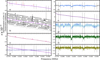 |
Fig. 4 Description of step 2 of the data processing algorithm (see middle part of Fig. 2). The data presented here correspond to the 19th sub-band of the data set presented in Fig. 3. The black dotted lines represent the mask around the expected lines. The different colours represent the sub-band at each step of the processing (described in the middle part of Fig. 2). (a) The red (resp. purple) spectrum is before (resp. after) the ‘RFI mitigation 2’ step. (b) The purple spectrum is the sub-band being processed, the black spectra are the neighbouring sub-bands used to assess the general shape. The gray sub-band has been discarded. (c) The pink line is the median of the black and purple sub-band in panel (b), and the black dotted line is the median smoothed by a Savitzky–Golay filter. (d) The purple (resp. navy blue) spectrum is before (resp. after) the ‘flattening 2’ step. (e) The navy blue (resp. azure blue) spectrum is before (resp. after) the ‘RFI mitigation 3’ step. In this case, RFI was removed at 13.92 and 13.96 MHz. (g) The azure blue (resp. light blue) spectrum is before (resp. after) the ‘flattening 3’ step. The light blue (resp. green) spectrum is before (resp. after) the ‘RFI mitigation 4’ step, and the black dotted line is the green spectrum smoothed by a Savitzky–Golay filter. (i) Black line indicates the zero baseline and the olive green spectrum is the final flattened and cleaned sub-band. |
3.1.3 Whole spectrum
Finally, we concatenated all 384 sub-bands to build a global spectrum spanning from 10 to 85 MHz, to which we applied a final 3 rms clipping procedure. The goal was to remove remaining spikes located on the edges of the sub-bands, as well as to mitigate remaining RFIs according to the global noise level of the spectrum. We computed the rms values over a sliding, 2048 channels-wide window along the whole spectrum. These values are used as a metric for the ‘quality’ of each frequency channel in the averaging and stacking procedures. This final step of the data processing is illustrated in Fig. 5.
3.2 Time averaging
The reduction pipeline is applied on each two-hours observation block. The resulting spectra are then averaged together (see Fig. 6i). We note that the RFI depend greatly on human activity and, thus, on the moment when the observations were performed. Two criteria were used to assess the quality of an observation block before time averaging: the percentage of frequency channels flagged out as RFI, and the rms of the spectrum. The former is mainly influenced by whether the observation was performed during the day or during the night, with up to an average of 80% of the spectrum flagged for observation around noon, and above 30% between 5 am and 7 pm. Heavy flagging of day-time spectra keeps the rms on the remaining frequency channels stable throughout the day. Neither of these criteria are impacted by the day, month, or year of the observation. For Cygnus A, the mean rms value of the optical depth noise goes from 3 × 10⁻⁴ to over 8 × 10⁻⁴, depending on the moment the observations were performed. For Cassiopeia A, the mean rms value of the optical depth goes from 4 × 10⁻⁴ to about 7 × 10⁻⁴.
A blind averaging procedure would allow for the narrow-band sporadic RFI to propagate throughout all the spectra. As a result, we used the rms of the spectra computed on a sliding window of length = 2048 frequency channels, as a way of assessing the quality of a spectrum. We compute the weight kυ,S for each frequency channel υ of each spectrum, S, as
 (1)
(1)
where συ,S is the rms of the spectrum S at the frequency υ. To account for the Doppler effect due to the rotation of the Earth with respect to the kinematical local standard of rest, we realigned each spectrum on a reference frequency grid, before averaging4. The weighted average of the spectra is computed to create a single spectrum with an increased S/N for further analysis.
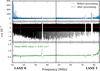 |
Fig. 5 Description of the step 3 of data processing (see bottom panel of Fig. 2). The black vertical line shows the separation between lane 0 and lane 1. The top panel compares the flat spectrum before (blue) and after (black) the mitigation process. The middle panel is a zoom on the black spectrum. The red dashed-dotted line shows the zero baseline. The vertical spikes are detections of Cα RRLs. The bottom panel shows the value of the rms computed in a sliding window along the spectrum. The holes in the spectrum (at 35 MHz, 73 MHz and 79 MHz) are flagged regions contaminated by unmanageable RFI pollution during this observing block. |
3.3 Stacking
The goal of stacking is to increase further the S/N. However, as the shape (both peak and width values) of the lines depends on the frequency of the transition (see Sect. B.1), the stacking procedure (see Fig. 6ii) tends to cancel out the specificities of each transition. Hence, this step is aimed at achieving a balance between a sufficient S/N to ensure a detection and as little stacking as possible to keep the line profiles intact. The number of lines included inside the stacks depends on the source and on the frequency, as the rms of the data is higher on the edges of the spectrum. To maintain the same S/N throughout the whole spectrum, we needed to stack together more lines at lower frequencies.
We preselected a generic set of subsequent lines, whose size depend on the frequency. We then filtered out heavily polluted lines (by RFI or a poor bandpass) to prevent propagation of artifacts in the final stack. To automatically detect these heavily polluted lines, we applied the following procedure to the preselected lines for the stacking:
Each line of the preselection is convolved with a generic Voigt profile, whose characteristics (width and depth) depends on the source.
The convolved lines are interpolated to a common reference grid. This step ensures that all lines are aligned on the same velocity scale, facilitating accurate comparison and combination;
Each convolved line is compared to a median reference line derived from the preselection. To assess the similarity between each convolved line and the reference, we use the R2 coefficient of linear correlation, and the ratio between the convoluted line and the reference; - Lines that show poor correlation (R2 < 0.7 or ratio greater than 1.3) with the reference (based on the similarity assessment) are identified as outliers. These outliers are excluded from further analysis to prevent them from skewing the results;
After removing outliers, a new median reference line is calculated from the remaining lines. This refined median line represents a cleaner and more accurate average of the spectral lines.
The process is reiterated with the refined median reference line until no outliers are detected.
Finally, a visual assessment was applied on the remaining lines, in order to ensure the highest quality for the detections. Towards Cassiopeia A, the lines removed through visual assessment account for∼30% of the discarded lines. Towards Cyg A, the S/N was too low for non-stacked spectra, making it irrelevant to try and convolve them with a Voigt profile. We applied only the visual assessment for this source.
We eventually applied the stacking procedure. First, each individual line is converted from a frequency axis to a velocity axis. Then, every line within a given stack is interpolated to a common velocity grid, defined by the coarsest grid. Finally, the isolated lines are weighted by the inverse square of their rms noise values. In order to account for the uncertainty on the calibration of NenuFAR, we determined a minimal value for the rms, which was obtained by capping the S/N at a value of 6. Lines presenting a better S/N were kept, but with a weight value equivalent to S/N of 6. The weighted lines are then summed to obtain an average spectral line profile. The process of stacking is illustrated for Cassiopeia A in Fig. 7. The exact number of lines used in each stacks can be found in Table C.1.
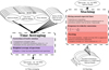 |
Fig. 6 Functional diagrams of the post-processing of the data. The left part of the figure describes the time averaging process described in Sect. 3.2. The right part illustrates the stacking process described in Sect. 3.3. |
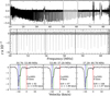 |
Fig. 7 Post-processing of the data, on the example of Cassiopeia A. Top panel represents the whole spectrum averaged over all observing blocks. The gray area is an example of three stacking selections. Middle panel is a zoom on the gray area. Vertical dashed lines encompass the three selections of lines to be stacked. The vertical spikes are Cα RRLs. Bottom panel shows the three stacks computed from the selections. Stacking allows for the detection of three velocity components. Their expected positions are determined from previous studies (Oonk et al. 2014, 2017; Salas et al. 2017) and are marked by the vertical coloured lines: blue (−47 km s−1), green (−38 km s−1) and red (0 km s−1). The mean S/N for these three stacks is about ~100 at ~1 km s−1 resolution. |
4 Results
From the stacked lines obtained from the procedure described in Sect. 3, we inferred five physical parameters for the diffuse clouds in the line-of-sight: the electron temperature, Te, the electron density, ne, the temperature of the radiation field, T0, the typical size of the cloud, L, and the mean turbulent velocity, υt. The procedure used to extract these parameters from the stacked lines is described in Appendix B. This section presents the results of these procedures for both sources: Cas A (Sect. 4.1) and Cyg A. (Sect. 4.2). For each source, we subsequently present the characteristics of the detected lines (in Sects. 4.1.1, 4.2.1), the results of the line fitting (in Sects. 4.1.2 and 4.2.2) and the evaluation of the physical parameters (in Sects. 4.1.3 and 4.2.3). Our physical estimates with their uncertainties are found in Table 2 and the optimisation results are presented in Fig. 8.
Best fit and uncertainties of the grid exploration.
4.1 Cassiopeia A
4.1.1 Detections
Cas A is the brightest radio source in the northern sky at 50 MHz(de Gasperin et al. 2020). It was observed by NenuFAR LT10 for 71.5 h. Towards this source, we detected 398 individual Cα lines between n = 426 and n = 826. Figure C.1 shows the resulting stacked spectra. The three known ISM clouds in the foreground of Cas A at radial velocities of –47, –38 (with typical optical depths of a few 10−3) and 0 km s−1 (with typical optical depths of a few 10−4, Oonk et al. 2017; Salas et al. 2017) are detected, at these opacity levels with NenuFAR. The –47 and –38 km s−1 components are variably blended throughout the observed band. This is due to a combination of two effects: the broadening of the lines at low frequencies (see Appendix B.1), and the dependency on the frequency of the conversion between frequency and velocity channels. The blending of the components, which occurs at frequencies lower than 24.34 MHz, makes it difficult to disentangle the absorption from these two components over a fraction of the observed band. We took these effects into account when performing the stacking described in Sect. 3.3. For this, we stacked together groups of ten to 30 transitions depending on the frequency (see Table C.1). To assess the robustness of our methodology, we compared our detections with the LOFAR LBA ones(Oonk et al. 2017; Salas et al. 2017). Our study significantly increases the S/N in comparison with those, as can be seen in Figs. 9i and 9ii. This allows for the detection of the 0 km s−1 component on a broader range of frequencies, and with less stacking needed. The S/N is increased by a factor of about four at the same velocity resolution, and by a factor of about two with the same integration time. We note a discrepancy between LOFAR and NenuFAR in the integrated line-to-continuum intensity of the lines (see Figs. 9i and 9ii). This difference is above the noise, and varies from a few percent at high frequencies to a few tens of percent at low frequencies. We discuss it in Sect. 5.1.
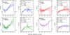 |
Fig. 8 Fit results for the clouds detected towards Cas A and Cyg A. The coloured points correspond to NenuFAR data obtained through LT10. The gray points correspond to LOFAR Data from Oonk et al. (2014); Salas et al. (2017). The coloured areas correspond to uncertainty range, determined as every parameter set that gives a distance within the lowest 30%. The dashed and coloured lines are the models for the optimal parameters of the minimisation. The boxed parameters are the optimal values of the minimisation. |
4.1.2 Line fitting and cloud identification
For Cassiopeia A, the primary approach is to fit simultaneously three Voigt profiles to account for the three velocity components. Two issues arise regarding the fitting. First, the depth of the CRRLs varies with frequency as per the theory, and this variation is different for each different velocity clouds, as they do not necessarily share the same physical parameters. This means that some velocity component might dominate the others in some parts of the spectrum. Moreover, as the size of the velocity channels widens as the frequency decreases, the velocity components blend below a certain frequency (around 40 MHz) until they are virtually indistinguishable (around 30 MHz). To manage these specificities, we adjusted the fitting prior and search bounds according to the principal quantum number, in order to provide a made-to-measure guide for the fitting algorithm:
For n below 560 (i.e. υ > 37.37 MHz), the centre of the Voigt profiles of the –47 km s−1 component was confined between −50 and −44 km s−1. The centre of the two other components were defined by their distance from the –47 km s−1 component: the −38 km s−1 and the 0 km s−1 must be respectively at (+ 9 ± 2) km s−1 and (+ 47 ± 2) km s−1 of the main velocity component.
For n above 560, we keep the same bound on the centre of the main Voigt profile, but the distance with the other components can vary by only 1 km s−1. Moreover, we force the line area of the –38 km s−1 component to be less or equal to a third of the line area of the –47 km s−1. The line area of the 0 km s−1 must be less than or equal to the –38 km s−1 component. This strategy is tailored to mitigate as much as possible the effect of the blending of the –47 and –38 km s−1. We also force a dynamic bound on the width of the lines: the Gaussian width must be almost constant (as the Gaussian width is supposed to be independent from the frequency, see Appendix B.1), and the Lorentzian width must be globally increasing.
Due to the blending, the uncertainties above n ∼ 600 are dominated by the inability for the curve_fit to differentiate properly the velocity components. To assess the uncertainty on the line width and the line integrated intensity, we applied a statistical method. A stacked line is composed of a set of consecutive transitions. For each stack, we selected 300 random subsets of transitions, of varying lengths, that we stacked and then fitted with the same methodology as described above. We extracted from these fits a value of the line width and integrated intensity for the three components. We then evaluated the line widths and integrated intensities, along with their uncertainties for each stack as the mean and 3 rms of the values from every subsets. We applied this methodology for each stacked line whose average quantum number was above 600. The results of the line fitting are available in Fig. C.1 and in Table C.2.
Following the approach described in Sect. B.2.3, we performed a cross-analysis of the CRRLs with dust clouds and CO in the corresponding line-of-sight. The dust distribution in the sightline of Cas A up to 1.25 kpc presents three main absorption peaks, at about 175, 280 and 350 pc from the Sun (middle panels of Figs. 10, 11). The CO spectrum averaged in a beam of 3.59° (corresponding to the beam of NenuFAR at 10 MHz) presents two components: a wider and stronger one between —60 and —20 km s−1 with a central velocity around −40 km s−1, and another one wide of about 15 km s−1 and with a central velocity of −3 km s−1 (top panels of Figs. 10, 11). The largest velocity component seems to harbour two distinct components, peaking at −40 and −50 km s−1. We related these components respectively to the −38 and −47 km s−1 clouds detected with CRRLs. We identified a spatial correlation in the plane-of-sky between the dust cloud located at a distance of 282 pc from the Sun, and the −47 and −38 km s−1 velocity components, as shown in Fig. 11. We measured a FWHM of 24 pc along the line of sight for this dust cloud. We were unable to identify two separate spatial structure corresponding to the two velocity components, and assumed the same prior L for both. Using the same methodology, we identify a correlation between the dust cloud located at 350 pc from the Sun and the 0 km s−1 velocity component of Cas A, as shown in Fig. 10. We measured a FWHM of 8 pc for this component.
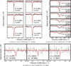 |
Fig. 9 Overplot of the lines detected towards Cas A (Figs. 9i, 9ii) and Cyg A (Fig. 9iii) for LOFAR LBA (black) and NenuFAR (red). The panels in Fig. 9i compare the detections of LOFAR LBA in the frequency range ~35 to ~68 MHz, from Oonk et al. (2017). The panels in Fig. 9ii compare the detection of LOFAR LBA from ~10 to ~35 MHz, from Salas et al. (2017). The panels in Fig. 9iii compare the detection of LOFAR LBA from ~35 to ~57 MHz, from Oonk et al. (2014). The top panel (LOW) presents the detections of LOFAR LBA in the frequency range ~33 to ~43 MHz, the middle panel (MID) presents the detection from ~39 to ~49 MHz and the bottom panel (HIGH) is the detections from ~44 to ~57 MHz. The detections from NenuFAR were rebinned to the same velocity resolution as LOFAR, and the same transitions were included in the stacks. |
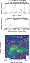 |
Fig. 10 Cloud identification for the 0 km s −1 component of Cas A. Top panel: CO spectrum averaged over the largest beam of NenuFAR. The gray line represents the whole spectrum. The coloured part is the sliced used to draw the intensity map in the bottom panel (see Dame et al. 2001). Middle panel: dust distribution along the sightline of Cas A (see Edenhofer et al. 2024). The gray line represents the sightline up to a distance of 1.25 kpc. The coloured part is the slice used to plot the contours in the bottom panel. Bottom panel: overplot of the intensity of CO and dust absorption in the plane of sky. The colour map is the 0th moment of the CO cube limited to velocities between −20 and 20 km s−1. The contours are the absorption of the dust located between 0.3 and 0.5 kpc from the Sun. The white filled circle represents the position and size of Cas A. The black dashed circles are the largest and smallest beams of NenuFAR (respectively 3.59° and 24.4′). |
4.1.3 Determination of the physical parameters
For the −47 km s−1 velocity component, we found a solution with optimal values estimated at ne = 2.7 × 10⁻² −3.9 × 10⁻² cm−3, with ne,opt = 2.7 cm−3, Te = 35-50 K, with Te,opt = 45 K and υt = 2.7-3.8 km s−1, with υt,opt = 3.3 km s−1. This solution is found for T0 = (1700 ± 100) K and L = 32.5-33.5 pc. From these values, we infer EMC II = 0.024-0.051 cm−6 pc, pth/k = 6.8-13.9 × 10³ Kcm−3 and pt∕ k = 0.6-6.5 × 10⁵ Kcm−3. These values are consistent with the prediction of Wolfire et al. (2003) for the neutral ISM of the Milky Way, of a thermal pressure pth ~ 10 × 103 K cm−3 that is dominated by the turbulent pressure. We also infer the total Doppler broadening to be between 4.5 and 6.3 km s−1. Overall, the measured parameters point towards a diffuse partially ionised phase of the ISM. The result of the grid search is presented in Fig. D.1. An overplot of the data points and the best fit is in panel a of Fig. 8.
The values inferred by Salas et al. (2017) for this cloud are ne = 2 × 10⁻² - 3.5 × 10⁻² cm−3, Te = 60-98 K, T0 = 1500-1650 K and pth∕ k = 11-21 × 103Kcm−3. Oonk et al. (2017) inferred pth∕ k = 19-29 × 103 K cm−3, pt∕ k = 1.8-2.0 × 10⁵ Kcm−3, a total Doppler broadening of 3.4 km s−1, EMC II = 0.042-0.070 cm−6 pc, ne = 3.5 × 10⁻² - 4.5 × 10⁻² cm−3, Te = 80-90 K, T0 = 1268-1484 K and L = 34.1-36.5 pc. Our estimates are in general agreement with LOFAR results. The difference in Doppler broadening is understandable due to the dependency of υt on the beam size (see Sect. 5.1). The slight differences between LOFAR and NenuFAR estimates are sufficiently small as to not impact the interpretation of the component as a diffuse partially ionised medium.
In contrast to Salas et al. (2017), who assumed the same physical properties for the two components, NenuFAR’s higher spectral resolution and S/N allowed us to distinguish differences between the −47 and −38 km s−1 clouds, For the latter, we found a solution with optimal values estimated at ne = 2.5 × 10⁻² cm−3, Te = 37-44 K, with Te,opt = 40 K and υt = 3.4-6.1 km s−1, with υt,opt = 4.7 km s−1. This solution is found for T0 = (1200 ± 100) K and L = 20–21 pc. From these values, we infer EMC II = 0.012-0.013 cm−6 pc, pth∕ k = 6.6-7.9× 10³ Kcm−3, pt∕ k = 0.810.7 × 105 K cm−3 and a Doppler broadening between 5.7 and 10.8 km s−1. The thermal pressure inferred here is slightly below the expected value of ~10 × 103 Kcm−3. The turbulent pressure dominates over the thermal pressure, as expected. Again, our solution points to a diffuse and partially ionised medium. Oonk et al. (2017) found pth∕ k = 19-29 × 103 Kcm−3, pt∕ k = 6.68.6 × 105 Kcm−3, a total Doppler broadening of 6.8 km s−1, EMc II = 0.022-0.038 cm−6 pc, ne = 3.5 × 10⁻²−4.5 × 10⁻² cm−3, Te = 75-95 K, T0 = 1379-1635 K, and L = 17.0-20.2 pc.
Although there is a slight deviation between LOFAR’s and NenuFAR’s estimates in the analysis of both clouds, these differences are understandable as the data points from NenuFAR deviate from the ones from LOFAR (see panel b of Fig. 8). The differences in estimate are sufficiently small as to not impact the interpretation of the component as a diffuse partially ionised medium. We discuss this issue further in Sect. 5.1.
An overplot of the data points and the best fit is in Fig. D.2. The optimal modelling fits well the line width for quantum numbers below n ~ 600 and deviates afterwards. The uncertainty area generally encompasses the integrated area data points below n ~ 600. Above n ~ 600, the measure of the integrated line-to-continuum intensity collapses. This is due to the blending of the components, and the fact that the algorithm only sees one Voigt profile instead of two. In addition, at these quantum numbers, the Lorentzian wings are wider and blend with the continuum, resulting in the algorithm potentially underestimating their contribution to the intensity. Thus, the decrease in the line intensity is not physical, and cannot be reproduced by our modelling, so it should not impact the optimisation process. Panel b of 8shows indeed that the optimisation fitted mostly the left part of the curves.
For the 0 km s−1 velocity component, we found a solution with optimal values estimated at ne = 1.3 × 10⁻²−1.5 × 10⁻² cm−3, with ne,opt = 1.4 cm−3, Te = 45-71 K, with Te,opt = 52 K, and υt = 1.7-5.6 km s−1, with υt,opt = 3.7 km s−1. This solution is found for T0 = (1000 ± 100) K, L = 14.5-15.5 pc. From these values, we infer EMC II = 0.002-0.003 cm−6 pc, pth∕ k = 4.2-7.6 × 10³ Kcm−3, pt∕ k = 0.1-5.4 × 10⁵ Kcm−3 and a Doppler width between 2.9 and 9.3 km s−1. The thermal pressure inferred here is slightly below the expected value of ~10 × 103 K cm−3. The turbulent pressure is higher, but the extremal values of the pressures are separated from each other by less than an order of magnitude. This suggests that this cloud is at the limits of a typical behaviour of a CNM cloud.
Although NenuFAR is the first instrument that enables physical constraints to be set on the 0 km s−1 component, Oonk et al. (2017) were able to measure a Doppler width of wD = 2.5 km s−1, which is slightly lower than our measurement. The results of the grid search can be found in Fig. D.3, and an overplot of the data points and uncertainty ranges in panel c of 8.
4.2 Cygnus A
4.2.1 Detections
Cyg A was observed by NenuFAR LT10 for 157.5 h. There is one single known ISM cloud in the foreground of Cyg A at radial velocities of 3.5 km s−1(Oonk et al. 2014), with typical optical depths of a few 10−4. This is why we chose to stack together groups of 30–50 transitions depending on the frequency, ending up in eleven usable detections. The results are shown in Fig. C.2, and the characteristics of the detected lines are listed in Table C.1. We compare our results with the LOFAR LBA ones from(Oonk et al. 2014). As for Cas A, our study improves the S/N (see Fig. 9iii). When stacking the exact same transitions as Oonk et al. (2014), and rebinning our data to the LOFAR LBA frequency resolutions, we obtained a higher S/N than the LOFAR LBA one by a factor 10, and by a factor of three for the same integration time. In terms of optical depth, we note that the discrepancy between LOFAR LBA and NenuFAR is much less important towards Cyg A than towards Cas A (see Fig. 9iii), for reasons that we discuss in Sect. 5).
4.2.2 Line fitting and cloud identification
For Cygnus A, we rebinned every spectrum by a factor of 4, to improve the S/N. The fit was achieved blindly, without prior knowledge or bounds. The results of the line fitting are available in Fig. C.2. The cloud identification method (see Appendix B.2.3) revealed no CO cloud towards Cyg A, but the dust map analysis revealed a cloud crossing the line-of-sight at the LSR velocity of 3.5 km s−1. This cloud has an extinction FWHM of 12 pc (see Fig. 12), and is located at 70 pc from the Sun. We used this value as a prior on L for the grid exploration.
4.2.3 Determination of the physical parameters
We found a solution with optimal values estimated at ne = 1.6 × 10⁻² - 2.7 × 10⁻² cm−3, with ne,opt = 1.8 cm−3, Te = 57159 K, with Te,opt = 77 K, and υt = 6.6-9.3 km s−1, with υt,opt = 7.9 km s−1. This solution is found for T0 = (1600 ± 100) K, L = 7.5-8.5 pc. From these values, we infer EMC II = 0.0020.006 cm−6 pc, pth∕ k = 6.5-30.7 × 10³ K cm−3 and pt∕ k = 2.0-27.0 × 10⁵ K cm−3. These values are consistent with the prediction of Wolfire et al. (2003) for the neutral ISM of the Milky Way, of a thermal pressure pth ~ 10 × 103 Kcm−3 that is dominated by the turbulent pressure. Oonk et al. (2014) conducted an analysis of CRRLs towards Cyg A using LOFAR LBA, and found optimal values of Te ~ 110 K with uncertainty ranges from 50 to 500 K, which are compatible with our results. The electron density from LOFAR is found at ne ~ 6 × 10⁻²cm−3 with uncertainties from 0.005 to 0.07 cm−3, encompassing our results. They estimated EMC II ~ 0.001 cm−6 pc, giving the same order of magnitude as our study. They also found rough estimates of T0 ~ 2700 K, a Doppler width of ~10 km s−1 and pth/k ~ 40 × 103 Kcm−3. Given the range of the quantum numbers (n ≳ 500), they assumed the line broadening to be only in Lorentzian regime, therefore the turbulent velocity was estimated using observations at higher frequencies. However, the data points acquired by NenuFAR indicate that the shift from Doppler dominated to Lorentzian regime happens around n = 580, indicating that LOFAR’s data points were not completely in the Lorentzian dominated region.
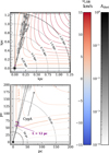 |
Fig. 12 Cloud identification for the 3.5 km s−1 component towards Cyg A. Both panels are an overplot of the dust distribution in gray (Edenhofer et al. 2024) and theoretical LSR velocities in blue and red contours (Reid et al. 2019). The largest beam of NenuFAR is marked in black dotted lines. The Sun is represented by the black cross. Top panel: overview of the sightline up to 1.25 kpc from the Sun. The gray contours correspond to the most prominent clouds in the beam of NenuFAR. Bottom panel: zoom on the close vicinity, up to 200 pc from the Sun. The purple cloud crosses the beam towards Cyg A at the expected velocity of 3.5 km s−1. |
5 Discussion
There are several limitations to our study, which are discussed them in this section. In Sect. 5.1, we focus on the consequences of differences in the beam size between LOFAR and Nenu-FAR. In Sect 5.2, we describe the multimodality and intrinsic degeneracies of the five-parameter model we used to describe CRRLs.
5.1 Beam effects
The discrepancy between the LOFAR and NenuFAR analyses (see Fig. 9) may be due to beam effects. In Salas et al. (2017),Oonk et al. (2017) and Oonk et al. (2014), the observations were performed in imaging mode with a field of view varying from 5′ to 23′, depending on the frequency. The current beam of Nen-uFAR varies between 25.2′ at 85 MHz and 3.59° at 10MHz. Figs. 13 and 14 shows a quantitative analysis of beam (top panel) and filling factor (bottom panel) differences between NenuFAR and the different setups used with LOFAR. We identified three possible effects from these differences.
First, the observed mean turbulent velocity υt increases with the size of the beam, as described by Gordon & Sorochenko (2002). This is because a larger beam encompasses a wider diversity of spatial structures hence of inner motions, generally leading to a higher turbulent velocity. A greater mean turbulent velocity increases the Doppler broadening, and therefore raises the left part of the curve (corresponding to low n values and high frequencies) of ∆υ as a function of n that corresponds to the Doppler-dominated frequencies. This is what we observed towards Cas A and Cyg A (see Fig. 8).
Second, we suspect some dilution effect due to the differences in beam sizes. In order to observe CRRLs in absorption, the diffuse ISM needs to be in the foreground of a radio source. As the radio source is resolved in neither cases and for neither instruments (see Fig. 13), we would expect the lines to have a similar depth for both instrument. This is the case towards Cyg A (see Fig. 9iii), but not towards Cas A, especially at low frequencies (see Figs. 9i and Figs. 9ii). The difference between LOFAR and NenuFAR towards Cas A suggests that the background against which we see the CRRLs is actually resolved, and not similarly encompassed by the beams of the instruments. As this dilution effect is more prominent towards Cas A than Cyg A, the fact that Cyg A is located farther from the Galactic plane than Cas A, points that the Galactic Plane Background is a strong enough radio source for CRRLs detections. However, we suspect that the exact change in line strength between the instruments depends on the foreground and background gases configurations.
Third, NenuFAR also presents grated lobes due to the hexagonal grid of the MAs (see Sect. 2.1, Fig. 1). The grating effect is more prominent at higher frequencies, with no effect at all visible below 27.3 MHz5. The grating lobes could affect the lines due to contamination by other bright sources that are not in the direction of the main target. As a result, new velocity components could become visible to NenuFAR by entering the grating lobes throughout the night, which can induce line blending if the new velocities are too close to the ones we observe. However, Fig. 14 shows that the filling factors of NenuFAR and LOFAR (which does not present grating lobes) are closer at high frequency. Thus, we considered that the grating lobes effect is negligible in our case.
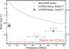 |
Fig. 13 Frequency dependence of beam sizes for NenuFAR and LOFAR, shown alongside the angular size of Cas A. The LOFAR beam is represented for the two CRRLs experiment: Salas et al. (2017) (circles) and Oonk et al. (2017) (squares). Oonk et al. (2017) cropped the images from LOFAR in squares whose sizes are fixed in two frequency windows. Salas et al. (2017) cropped the images from LOFAR in circles centred on Cas A, with continuous values for its diameter. The Nenu-FAR beam size function is shown with the solid line. The red dotted line represents the angular extension of Cas A at radio frequencies (Green 2014). The source is spatially resolved for neither setups, at any frequency. |
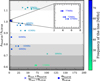 |
Fig. 14 Ratio of the line intensities towards Cas A between observations with NenuFAR and with LOFAR as a function of beam ratio. The crosses represent the filling factor ratios for Cas A and the dots represent the ratio of angular resolutions for the two experiments. If at a given frequency a dot and a cross are close to each other, then the filling factors are similar for both instruments, meaning a less prominent dilution effect between both experiments. The colour scale indicates the central frequency of the lines. The ratio of the line intensities follows the tendency of being farther from one at lower frequencies. The differences in filling factor follow the same tendency. |
5.2 Multimodality
In this section, we discuss the structure of the five-dimensional (5D) physical parameter space (as illustrated in Figs. D.1 through D.4). We also present the impact of multimodality on the evaluation of physical constraints. The best-constrained parameter in the 5D parameter space is the turbulent velocity. The optimal value of υt does not depend on the local minimum we look at and is very stable throughout the grid search. As shown in Fig. 15, for a given ne, the probability density for Te forms a bell curve around a Te,opt. The overall structure for the parameter Te is therefore a combination of bell curves: one for each different ne comprised in the 30% uncertainty limit. We generally found only a few solutions for ne, and the different bell curves for Te are relatively close to each other, leading to a total uncertainty of less than 10 K in some cases. The values chosen for T0 and L seem to influence the optimal values of ne and Te and not the general structure of the solutions. The parameter L impacts the value of ne and hence also the positions of the curve bells of Te (see Fig. 15), whereas T0 seems to lightly influence the position peak of υt, resulting in a more or less spread bell curve for υt.
The complex nature of the parameter space we study as well as the intrinsic degeneracy of the optimisation problem make it difficult to conduct a proper minimisation methodology. We are currently looking to improve this aspect of our analysis, which is a work in progress that is beyond the scope of this article.
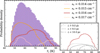 |
Fig. 16 Illustration of the influence of the parameters ne and L on the optimal value found for Te, for Cygnus A. The purple histogram represents all the values of Te that give |


6 Concluding remarks
We have shown that NenuFAR can be used to quantitatively study RRLs in the lowest observable frequency range to enhance our understanding of the diffuse ISM. More specifically, we used CαRRLs as a diagnostic tool to provide constraints on the electron density, ne, and electron temperature, Te in four different diffuse clouds of the ISM. Using the NenuFAR telescope’s low-frequency capabilities, we conducted observations of the two brightest radio sources of the northern sky: Cassiopeia A and Cygnus A. Through a meticulous data processing pipeline, we removed radio frequency interference and enhanced the S/N, resulting in high-quality spectral line profiles. This process allowed us to detect numerous carbon recombination lines, with Cassiopeia A yielding 398 lines, significantly improving upon previous studies. The lines towards Cygnus A lines are fainter and require extensive line stacking. Upon stacking, we obtained 11 usable lines towards Cyg A and 28 towards Cas A.
NenuFAR has significantly advanced the study of CRRLs by providing unprecedented sensitivity (of ~2 Jy at 50 MHz, for a two-hour integrating time at resolution) and broader frequency coverage in the 10–85 MHz range, at an unprecedented spectral resolution of 95 Hz. This work demonstrates NenuFAR’s ability to resolve finer details in CRRL profiles, achieving an improved S/N by a factor of four to ten compared to similar observations with LOFAR. The study addressed blending challenges and discrepancies in line intensities through meticulous data reduction and analysis, establishing a new benchmark for low-frequency radio observations. These advancements provided refined measurements of physical properties, such as the electron density and temperature, in line-of-sight clouds.
Furthermore, the methodology developed includes robust RFI mitigation and adaptive line-stacking techniques. It sets a precedent for future studies in diffuse ISM characterisation. Future improvements will focus on automating parts of the data pipeline and extending observations to additional sources. Overall, this study positions NenuFAR as a transformative tool in low-frequency radio astronomy, paving the way for more comprehensive studies of Galactic and extragalactic CRRLs.
We inferred physical parameters for the four ISM clouds detected towards Cas A and Cyg A. The first cloud was detected towards Cas A at a central LSR velocity of −47 km s−1. Our best-fit model was achieved for Te = 45 K, ne = 0.027 cm−3, T0 = 1200 K, L = 33.0 pc, and υt = 3.3 km s−1. From these values, we derived EM CII = 0.024 cm−6 pc, pth/k = 8.7 × 10³K cm−3, and pt∕ k = 3.4 × 10⁵K cm−3. The second cloud was detected towards Cas A at a central LSR velocity of −38 km s−1. Our best-fit model was achieved for Te = 40 K, ne = 0.025 cm−3, T0 = 1200 K, L = 20.5 pc, and υt = 4.7 km s−1. From these values, we derived EMCII = 0.013 cm−6pc, pth∕ k = 7.1 × 10³ K cm−3, and pt∕ k = 6.4 × 10⁵ Kcm−3. The third cloud was detected towards Cas A at a LSR velocity of 0 km s−1. Our best-fit model was achieved for Te = 52 K, ne = 0.014 cm−3, T0 = 1000 K, L = 15.0 pc, and υt = 3.7 km s−1. From these values, we derived EMCII = 0.003 cm−6 pc, pth∕ k = 5.2 × 10³K cm−3, and pt∕ k = 2.2 × 10⁵ Kcm−3. The fourth cloud was detected towards Cyg A at a LSR velocity of 3.5 km s−1. Our best-fit model was achieved for Te = 77 K, ne = 0.018 cm−3, T0 = 1600 K, L = 8 pc, and υt = 7.9 km s−1. From these, we derived EMC II = 0.003 cm−6 pc, pth∕ k = 9.9 × 10³ Kcm−3, and pt∕ k = 13.0 × 10⁵ K cm 3. These results are generally compatible with previous LOFAR studies and present typical values for diffuse partially ionised ISM phases.
The complexity induced by line blending and the intrinsic degeneracy of the physical modelling highlights the importance of using different observational techniques in making parameter estimations. Discrepancies observed between LOFAR and Nen-uFAR can be attributed to differences in the beam size and field of view, which may lead to increased turbulent velocities and/or a dilution effect, impacting the line intensity, seen in Cas A in particular. The turbulent velocity emerged as the most stable parameter throughout our analysis. For every cloud, the probability distribution of the electron temperature exhibited a bell curve influenced by the input values for T0 and L.
Acknowledgements
This work made use of Astropy (http://www.astropy.org) : a community-developed core Python package and an ecosystem of tools and resources for astronomy (Astropy Collaboration 2013, 2018, 2022). The authors acknowledge the support of the Programme National ‘Physique et Chimie du Milieu Interstellaire’ (PCMI) of CNRS/INSU with INC/INP cofunded by CEA and CNES. This paper is based on data obtained using the NenuFAR radiotelescope. NenuFAR has benefited from the funding from CNRS/INSU, Observatoire de Paris, Observatoire Radioastronomique de Nançay, Observatoire des Sciences de l’Univers de la Région Centre, Région Centre-Val de Loire, Université d’Orléans, DIM-ACAV and DIM-ACAV+ de la Région Ile de France, and Agence Nationale de la Recherche. We acknowledge the collective work from the NenuFAR-France collaboration for making NenuFAR operational, and the Nançay Data Center resources used for data reduction and storage. This project has received funding from the French Agence Nationale de la Recherche (ANR) through the projects COSMHIC (ANR-20-CE31-0009) and COSMHIC_Ukraine (ANR-20-CE31-0009-03). AB acknowledges financial support from the INAF initiative ‘IAF Astronomy Fellowships in Italy’. J.R.G. thanks the Spanish MCINN for funding support under grant PID2023-146667NB-I00.
Appendix A Discarding anomalous sub-bands in the correction of a given sub-band
We denote by Si(υ) the intensity in the i-th sub-band we want to correct: the set of sub-band used to compute the average is Si-5 to Si+5. So as to not spread RFI or distortions of the baseline throughout the 11 sub-bands, we flag those who differ from the sub-band we want to clean. To determine if a sub-band from the set {Sk}k∈[i-5,i+5] is significantly different from Si, we apply a statistical criterion: the level of distortion of Si is assessed by computing the two-norm of Si, defined by the square root of the integral of the squared sub-band:
 (A.1)
(A.1)
We then assess the level of dissimilarity of each (Sk)k∈[i-5,i+5] to Si by computing the square of the two-distance between Sk and Si:
![Mathematical equation: \forall k \in [i-5, i+5], \ k\neq i, \ \| S_\mathrm{k} - S_\mathrm{i} \|_2^2 = \int (S_\mathrm{k} - S_\mathrm{i})^2 \mathrm{d}\nu](/articles/aa/full_html/2025/09/aa55085-25/aa55085-25-eq18.png) (A.2)
(A.2)
We removed every sub-band with a dissimilarity level above 5% of the distortion level of the original sub-band. This criterion was chosen empirically. As more distorted sub-bands tend to have neighbours also presenting distortion, it can happen that a median sub-band baseline cannot be generated this way. In this case, we simply flag out the Si sub-band. The resulting potential baseline deformation are dealt with in a subsequent flattening step. The median of the sub-bands that have not been flagged is smoothed using a Savitzky-Golay filter (dotted black line in the third panel of Fig. 4), and subtracted from Si. We use Si′ to denote the result of the subtraction (blue line in the fourth panel of Fig. 4).
Appendix B Theory of line profiles and line fitting
The shape of low-frequency RRLs can be used as a probe of the physical conditions of the diffuse ISM in which they are produced. In Sect. B.1, we present the theory of RRLs and to what extent they relate to the physical parameters of the ISM. In Sect. B.2 we describe how we used this theory to constrain the physical parameters of ISM in the sightline of our specific sources.
B.1 Line profile: Theory
In the diffuse ISM, the recombination of ions and electrons forms atoms whose electrons are in levels with high principal quantum numbers (n). These newly bound electrons decay from level to level, radiating photons in form of spectral lines in the process. When these lines appear in the radio range, so-called RRLs are generated, that is after the de-excitation of an atom in a Rydberg state from the electronic quantum state n to a lower electronic quantum state n′. Here, we study CRRLs and we focus on the α transition (i.e. from n + 1 to n) with n ∈ [400, 850]. As described in Salgado et al. (2017b), for this range of n and for the physical conditions of CNM, there are RRLs seen in absorption. The frequency of a recombination line is given by, for instance, Gordon & Sorochenko (2002):
 (B.1)
(B.1)
with R∞ = 109 732.30 cm−1 (the Rydberg constant for the carbon atom) and mH and me the masses of the hydrogen atom and the electron.
We use a Voigt profile to model the shape of the line, as in Gordon & Sorochenko (2002), which is described by three parameters, namely the integrated optical depth and the Gaussian and Lorentzian widths. In turn, these parameters depend on the physical conditions of the diffuse ISM that we want to constrain. In this section, we detail the equations used to infer the physical conditions of diffuse ISM clouds from the shape of recombination lines.
Voigt profile. A Voigt profile is the convolution product of a Lorentzian profile and a Gaussian (Doppler) profile. We performed the fitting using the astropy.modelling.Voigt1D function from the astropy project6, in which the Voigt profile is described by four independent parameters: its central velocity υ0, the amplitude of the Lorentzian aL, the FWHM of the Gaussian wD and the FWHM of the Lorentzian wL. Let V be the Voigt profile function:
 (B.2)
(B.2)
with G0 the normalised Gaussian profile and L the Lorentzian of given amplitude. In practice, the υ0 value is set by the observations, leaving the Voigt profile to depend only on (aL, wL, wD). The FWHM of the Voigt profile wV depends on those of the Lorentzian and Gaussian ones, following Gordon & Sorochenko (2002):
 (B.3)
(B.3)
Integrated optical depth. For a line n → n′, Salgado et al. (2017a) provides the following description of the integrated line-to-continuum intensity:
 (B.4)
(B.4)
In this formula, ne and Te are the local density and temperature of electrons, while L is the size of the absorbing cloud; bn is a departure coefficient from local thermodynamic equilibrium (LTE) that depends on Te and ne, while βn,n′ is a correction factor for stimulated emission that has to be accounted for in the equations of statistical equilibrium; it also depends on Te and ne. Equation (7) from Salgado et al. (2017a) also accounts for a dependency on the local radiation field temperature, T0; however this dependency is negligible for n > 200 (see Prozesky & Smits (2018)). Figure (8) from Oonk et al. (2017) shows from observations of Cas A that varying T0 has little effect on the integrated area of the lines. For α transitions, the βn,n+1 factors are tabulated over a sample grid of Te and ne, with a constant T0 = 0 K(Salgado et al. 2017a).
Amplitude of the Lorentzian. The amplitude of the Lorentzian can be inferred from the line integrated intensity An and the FWHM of the Lorentzian and Gaussian profiles (Gordon & Sorochenko 2002):
![Mathematical equation: \begin{array}{cl} a_\mathcal{L}(A_{\rm n},w_\mathcal{L},w_\mathcal{D}) & = \displaystyle \frac{A_{\rm n}}{p(w_\mathcal{L},w_\mathcal{D})\times w_\mathcal{V}(w_\mathcal{L},w_\mathcal{D})} \vspace{2mm} \\ \text{with } p(w_\mathcal{L},w_\mathcal{D})&=(1.57 - 0.507 \exp{[-0.85 w_\mathcal{L}/w_\mathcal{D}]}). \vspace{2mm}\\ \end{array}](/articles/aa/full_html/2025/09/aa55085-25/aa55085-25-eq23.png) (B.5)
(B.5)
Full width half maximum of the Lorentzian. Three distinct physical effects control the width of the Lorentzian component wL: radiation broadening, natural broadening, and pressure (or collisional) broadening. Each of them is characterized by a width wrad, wnat, wcol such that wL = wrad + wnat + wcol. The radiation broadening can be modelled by:
 (B.6)
(B.6)
In this expression, T0 is the brightness temperature of the ambient radiation field Tb(υ) at a given frequency υ0,α, representative of the observation range. α is then the spectral index of the radiation field variation in the same frequency range, such that:
 (B.7)
(B.7)
We chose α = −2.6 and υ0,α = 100 MHz, consistently with Salgado et al. (2017a) and Salas et al. (2017). In addition to this, the natural broadening depends only on n through:
 (B.8)
(B.8)
Finally, the pressure (or collisional) broadening depends on Te and ne :
 (B.9)
(B.9)
where α and γ are tabulated in Salgado et al. (2017b).
Full width half maximum of the Gaussian: Doppler broadening. The Gaussian shape in the Voigt profile is physically due to the Doppler broadening. The Doppler effect in diffuse clouds originates in the combined action of the thermal and non-thermal motions. The non-thermal motions include disordered motions, as well as potential ordered-motions such as infall, rotation, or shocks. For simplicity, we refer to all the non-thermal motions as ‘turbulence’. Thus, the FWHM of the Gaussian is the quadratic sum of these two effects (Salgado et al. 2017b):
 (B.10)
with MC as the atomic mass of carbon. The average turbulent velocity υt is the mean of the turbulent motions within the telescope beam with respect to the angular extent of the observed cloud. Hence, it depends greatly on the beamwidth of the instrument as well as the scale of the ISM phase along the line of sight.
Dependencies. Overall, the dependencies of the observables (i.e., the parameters of the line shape: An, wL,n, wD,n, aL,n) on the physical parameters (Te, ne, υt, T0 and L) can hence be summarised as
 (B.11)
Additional diagnostics. From these physical parameters, we are able to infer additional diagnostic tools, namely the emission measure of CII EMCII, the thermal pressure pth and the turbulent pressure, pt.
As the ionisation energy of carbon is lower than for hydrogen and helium (11.26 eV, 13.6 eV and 24.59 eV respectively), we assume carbon to be the main ionised species in the observed PDRs. Hence we have nC II ≃ ne, and EMC II can be inferred from the measured parameters ne and L (see Eq. B.12).
 (A.12)
We also computed the thermal pressure pth of the observed clouds, assuming that the electrons are at thermal equilibrium, hence, Te = T. As done in Oonk et al. (2017), we assume that carbon is fully ionised, and the C II fraction is x(C II) ≃ 1.4 × 10⁻⁴ in diffuse lines of sights (Sofia et al. 2004).
 (B.13)
Finally, we compute the turbulent pressure pt from the measured υt, using the equation from Lequeux (2002):
 (B.14)
with mH the mass of the hydrogen atom. Thus, we have:
 (B.15)
For the neutral phase of the Milky Way,(Wolfire et al. 2003) predicts that the turbulent pressure dominates over the thermal pressure, which is typically ~10 × 103 K cm−3.
B.2 Line profile: Fitting
For each source, we began by fitting individually the stacked lines introduced in Sects 4.1 and 4.2 with Voigt profiles. We then determined the profile broadening and integrated intensity. We subsequently studied the variation of these two parameters as a function of the average principal quantum number of the transitions present in the stacks n. This average quantum number is the one that is used to compute the departure coefficients as well as the radiative, natural and collisional widths. Finally, we ran through a grid of physical parameters to find which combination of defining parameters (Te the electron temperature, ne the electron density, T0 the temperature of the local radiation field, υt the local mean turbulent velocity and L the depth of the cloud along the line-of-sight) best reproduces the observed variation as a function of n.
B.2.1 Fitting the shape of the lines
The algorithm iterates over the individual spectral stacks obtained from observations. Each iteration involves:
Signal detection: we calculate a S/N threshold and the algorithm determines whether a significant signal is present in the data. We deem the signal significant if the S/N is above 3. To compute the signal value, we integrate the spectral line. To compute the noise value, we mask the line out of the spectral stack, and we compute the rms of the remaining frequency channels. We then integrate this value over the frequency span of the spectral stack.
Voigt profile fitting: if a signal is detected, the algorithm fits a Voigt profile to the spectral line using the curve-fitting function (curve_fit) of the scipy.optimize module from scipy7 (Virtanen et al. 2020). Generally the Voigt fitting step does not require any prior knowledge of the signal. However, for lines of sight with blended velocity components, constraints can be added to guide the algorithm through the curve-fitting (as for Cas A, see Sect. 4.1.2).
Parameter extraction: the line width and integrated intensity are extracted from the fitted Voigt profile. The fitting uncertainties are determined by integrating the residuals of the fit. Again, for lines of sight with blended velocity components, we had to adopt a different procedure (see Sect. 4.1.2 for Cas A).
Linear ranges and coarseness of the grids explored to infer physical parameters.
B.2.2 Extracting the physical parameters
We computed the χ2 distance between a model and the observation based on line width and integrated intensity. For a given target, we call nS the number of stacks for which we extracted these two quantities. Let A be the list of observed integrated intensities, Â the list of modelled integrated intensities, and  the variance on the measure of A, as defined in Sect. B.2.1. Let wv be the list of observed profile widths,
  the list of modelled profile widths, and
  the variance on the measure of wv. The χ2 distance is:
 (B.16)
We then evaluated the reduced χ2, noted χ r2, by dividing by the number of degrees of freedom of the optimisation problem:
 (B.17)
with nP = 5 the number of independent parameters of the physical modelling. We used 2× ns for the total number of data points as we extracted two observables from each velocity component in a stack (wv and A).
The parameters (Te, ne, T0, υt) are systematically explored within predefined linear ranges chosen to be representative of the CNM that we initially sought after. The L parameter is explored around a prior determined by a cloud identification method, described in Sect. B.2.3. The range and coarseness of the initial grid are in Table B.1.
Exploration of the parameter grid revealed that the modelling does not provide significant constraints on L and T0, leading to the existence of multiple local minima. The preliminary explorations show that υt is the same in every local minimum, whereas the values found for Te and ne are shifting when varying L or T0. In order to lift part of the degeneracy, we chose to restrict the exploration of the finer parameter grid to values close to the global minimum of T0 and L obtained during the broad exploration. For each combination of parameters within the pre-defined range, model predictions are compared against observed data using χ r2. In a second step, we refined the grid around the detected minima. The maximum precision to which the grid is refined for each parameter is detailed in Table B.1.
B.2.3 Cloud identification
We performed a cross-analysis of CRRLs from NenuFAR, dust clouds in a radius of 1.25 kpc from the Sun, and CO PPV cubes towards each source in order to locate the observed clouds along our lines-of-sight. The 3D dust maps are from the Gaia DR3(Edenhofer et al. 2024), and CO data cubes are from the whole-Galaxy CO (1–0) survey from the 1.2 m Millimeter-Wave telescope at the Center for Astrophysics | Harvard & Smithsonian(Dame et al. 2001). This survey is a composite map with varying specificities. The map containing Cas A yields a spectral resolution of 0.65 km s−1 and and an angular resolution of 7.5’ meanwhile the map containing Cyg A has the same spectral resolution and an angular resolution of 15’. The cloud identification provides a meaningful prior for the grid search for the L parameter, as there is no a priori value for the CNM.
First, we searched in the Gaia DR3 maps if dust clouds were present in our lines of sight. For each of them, we found a number of clouds encompassed (totally or partially) in the beam of NenuFAR. The 3D nature of the map allowed us to measure the length of the dust clouds by measuring the FWHM of their absorption along the line of sight (see top panels of Figs. 10 and 11). It also allowed us to assess the structure of the clouds by projecting the 3D map on the plane of sky. Combining these informations, we were able to extract the structures in the plane of sky of each absorbing cloud along the line-of-sight separately, by projecting only the slices of the 3D absorption map that contained a given cloud. Then, for each source, we computed the CO spectrum averaged over the NenuFAR beam to identify common velocity components between CRRLs and CO. If we found CO emission at the same central velocity as the lines we detected in CRRLs, then we selected a slice of the CO cube containing the emission (see top panels of Figs. 10,11), and we computed its 0th order moment so as to assess the size and shape of a potential CO cloud at this velocity. Finally, we overlaid the projected maps of the dust clouds in the plane-of-sky with the 0th order moment in CO for different velocities, to compare the shapes of dust and CO clouds, and find potential matches (see bottom panels of Figs. 10 and 11).
In the absence of such a match, we compute the expected local standard of rest (LSR) velocity as a function of the heliocentric distance, based on the theoretical modelling of Reid et al. (2019) and the python module of Wenger et al. (2018). The methodology of Reid et al. (2019) is to first assume a circular galactocentric velocity, and to project the velocity vector on the heliocentric line-of-sight according to the galactic longitude and latitude of the source, as well as the Sun’s proper motion. Then, we check if a dust cloud in the beam whose LSR velocity is the one we detect with CRRLs.
The prior on L we obtain through this method is rudimentary because CO, diffuse and dusty clouds are not necessarily correlated. However, this method allowed us to identify a prior for every cloud, which our grid explored ±10 pc around the prior in steps of 1 pc.
Appendix C Detections and line fitting
Summary of the parameters of the stacking procedure for each source.
Measured line properties for C nα stacked recombination lines towards Cas A.
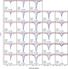 |
Fig. C.1 Every stack of lines detected towards Cassiopeia A used to extract physical parameters. The coloured lines are the results of the Voigt profile fitting algorithm. The blue lines correspond to the component at –47 km s−1, the green lines are the –38 km.s-1 component and the red lines are the 0 km s−1. The measured line properties can be found in Table C.3. |
Measured line properties for C nα stacked recombination lines towards Cas A.
Measured line properties for C nα stacked recombination lines towards Cyg A.
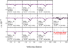 |
Fig. C.2 Every stack of lines detected towards Cygnus A used to extract physical parameters. The purple lines are the results of the Voigt profile fitting algorithm. |
Appendix D Result of the grid search
 |
Fig. D.1 Summary of the grid search for Cassiopeia A, component −47 km s−1. The top panel is the histogram of all the nodes of the final grid. The blue part of the histogram highlights the 30% of χ2 that are kept to evaluate the uncertainties. The bottom panels represent for each parameter the values that gives a χ2 distance comprised in the 30% range. |
 |
Fig. D.2 Summary of the grid search for Cassiopeia A, component −38 km s−1. The green part of the histogram highlights the 30% ofχ2 that are kept to evaluate the uncertainties. The bottom panels represent for each parameter the values that gives a χ2 distance comprised in the 30% range. |
 |
Fig. D.3 Summary of the grid search for Cassiopeia A, component −47 km s−1. The red part of the histogram highlights the 30% of χ2 that are kept to evaluate the uncertainties. The bottom panels represent for each parameter the values that gives a χ2 distance comprised in the 30% range. |
 |
Fig. D.4 Summary of the grid search for Cygnus A, component 3.5 km s−1. The purple part of the histogram highlights the 30% of χ2 that are kept to evaluate the uncertainties. The bottom panels represent for each parameter the values that gives a χ2 distance comprised in the 30% range. |
References
- Asgekar, A., Oonk, J. B. R., Yatawatta, S., et al. 2013, A&A, 551, L11 [NASA ADS] [CrossRef] [EDP Sciences] [Google Scholar]
- Astropy Collaboration (Robitaille, T. P., et al.) 2013, A&A, 558, A33 [NASA ADS] [CrossRef] [EDP Sciences] [Google Scholar]
- Astropy Collaboration (Price-Whelan, A. M., et al.) 2018, AJ, 156, 123 [Google Scholar]
- Astropy Collaboration (Price-Whelan, A. M., et al.) 2022, ApJ, 935, 167 [NASA ADS] [CrossRef] [Google Scholar]
- Bron, E., Roueff, E., Gerin, M., et al. 2021, A&A, 645, A28 [NASA ADS] [CrossRef] [EDP Sciences] [Google Scholar]
- Chowdhury, A., & Chengalur, J. N. 2019, MNRAS, 486, 42 [Google Scholar]
- Dalgarno, A. 2006, PNAS, 103, 12269 [NASA ADS] [CrossRef] [Google Scholar]
- Dame, T. M., Hartmann, D., & Thaddeus, P. 2001, ApJ, 547, 792 [Google Scholar]
- de Gasperin, F., Vink, J., McKean, J. P., et al. 2020, A&A, 635, A150 [NASA ADS] [CrossRef] [EDP Sciences] [Google Scholar]
- Edenhofer, G., Zucker, C., Frank, P., et al. 2024, A&A, 685, A82 [NASA ADS] [CrossRef] [EDP Sciences] [Google Scholar]
- Emig, K. L., Salas, P., de Gasperin, F., et al. 2019, A&A, 622, A7 [Google Scholar]
- Emig, K. L., Salas, P., de Gasperin, F., et al. 2020, A&A, 634, A138 [NASA ADS] [CrossRef] [EDP Sciences] [Google Scholar]
- Emig, K. L., Gupta, N., Salas, P., et al. 2023, ApJ, 944, 93 [NASA ADS] [CrossRef] [Google Scholar]
- Girard, J. N., & Zarka, P. 2023, A&A, 672, A80 [NASA ADS] [CrossRef] [EDP Sciences] [Google Scholar]
- Godard, B., des Forêts, G. P., & Bialy, S. 2024, A&A, 688, A169 [NASA ADS] [CrossRef] [EDP Sciences] [Google Scholar]
- Goicoechea, J. R., & Cuadrado, S. 2021, A&A, 647, L7 [NASA ADS] [CrossRef] [EDP Sciences] [Google Scholar]
- Gordon, M. A., & Sorochenko, R. L. 2002, Radio Recombination Lines. Their Physics and Astronomical Applications, 282 [Google Scholar]
- Green, D. A. 2014, Bull. Astron. Soc. India, 42, 47 [NASA ADS] [Google Scholar]
- Heays, A. N., Bosman, A. D., & van Dishoeck, E. F. 2017, A&A, 602, A105 [NASA ADS] [CrossRef] [EDP Sciences] [Google Scholar]
- Joblin, C., Bron, E., Pinto, C., et al. 2018, A&A, 615, A129 [NASA ADS] [CrossRef] [EDP Sciences] [Google Scholar]
- Lequeux, J. 2002, in Le Milieu Interstellaire (EDP Sciences) [Google Scholar]
- Liu, X., Liu, T., Shen, Z., et al. 2023, A&A, 671, L1 [NASA ADS] [CrossRef] [EDP Sciences] [Google Scholar]
- Mebold, U., & Hills, D. L. 1975, A&A, 42, 187 [Google Scholar]
- Morabito, L. K., Oonk, J. B. R., Salgado, F., et al. 2014, ApJ, 795, L33 [NASA ADS] [CrossRef] [Google Scholar]
- Oonk, J. B. R., van Weeren, R. J., Salgado, F., et al. 2014, MNRAS, 437, 3506 [Google Scholar]
- Oonk, J. B. R., van Weeren, R. J., Salas, P., et al. 2017, MNRAS, 465, 1066 [Google Scholar]
- Padovani, M., Galli, D., & Glassgold, A. E. 2009, A&A, 501, 619 [NASA ADS] [CrossRef] [EDP Sciences] [Google Scholar]
- Padovani, M., Ivlev, A. V., Galli, D., & Caselli, P. 2018, A&A, 614, A111 [NASA ADS] [CrossRef] [EDP Sciences] [Google Scholar]
- Peeters, E., Habart, E., Berné, O., et al. 2024, A&A, 685, A74 [NASA ADS] [CrossRef] [EDP Sciences] [Google Scholar]
- Prozesky, A., & Smits, D. P. 2018, MNRAS, 478, 2766 [NASA ADS] [CrossRef] [Google Scholar]
- Reid, M. J., Menten, K. M., Brunthaler, A., et al. 2019, ApJ, 885, 131 [Google Scholar]
- Salas, P., Oonk, J. B. R., van Weeren, R. J., et al. 2017, MNRAS, 467, 2274 [NASA ADS] [Google Scholar]
- Salas, P., Oonk, J. B. R., van Weeren, R. J., et al. 2018, MNRAS, 475, 2496 [Google Scholar]
- Salgado, F., Morabito, L. K., Oonk, J. B. R., et al. 2017a, ApJ, 837, 141 [Google Scholar]
- Salgado, F., Morabito, L. K., Oonk, J. B. R., et al. 2017b, ApJ, 837, 142 [Google Scholar]
- Sofia, U. J., Lauroesch, J. T., Meyer, D. M., & Cartledge, S. I. B. 2004, ApJ, 605, 272 [NASA ADS] [CrossRef] [Google Scholar]
- Stepkin, S. V., Konovalenko, A. A., Kantharia, N. G., & Udaya Shankar, N. 2007, MNRAS, 374, 852 [Google Scholar]
- Virtanen, P., Gommers, R., Oliphant, T. E., et al. 2020, Nat. Methods, 17, 261 [Google Scholar]
- Wenger, T. V., Balser, D. S., Anderson, L. D., & Bania, T. M. 2018, ApJ, 856, 52 [Google Scholar]
- Wolfire, M. G., McKee, C. F., Hollenbach, D., & Tielens, A. G. G. M. 2003, ApJ, 587, 278 [Google Scholar]
- Zarka, P., Denis, L., Tagger, M., et al. 2020, in 2020 XXXIIIrd General Assem bly and Scientific Symposium of the International Union of Radio Science, Institute of Electrical and Electronics Engineers (IEEE), Rome, Italy [Google Scholar]
- Zhou, P., Li, J.-T., Zhang, Z.-Y., et al. 2018, ApJ, 865, 6 [NASA ADS] [CrossRef] [Google Scholar]
Upon completion, NenuFAR will feature 96 MAs within a 400 m diameter core and eight remote MAs positioned at distances up to a few kilometers from the centre.
see https://nenufar.obs-nancay.fr/en/astronomer/ for additional technical details about the NenuFAR telescope.
We do not correct the Doppler shift within a two-hour observation because the Doppler shift between the first and last spectra, although it varies throughout the year, is at most of ~100 m/s, always below the spectral resolution of NenuFAR (~2.6 km/s at 10 MHz, ~335 m/s at 85 MHz).
All Tables
Linear ranges and coarseness of the grids explored to infer physical parameters.
All Figures
|
Fig. 1 Configuration of the NenuFAR telescope. Top panel: layout of all 96 mini-arrays forming the NenuFAR interferometer. Bottom panel: schematic layout of a mini-array showing the 19 inverted-V shape dual polarisations antennas. They are arranged in a 5.5 m triangular lattice forming a hexagon (from Girard & Zarka 2023). |
| In the text | |
|
Fig. 2 Functional diagram for the processing of L1 level data (see Sect. 3.1). The algorithm is split in three reduction layers: lane-by-lane (top, 2a, Sect. 3.1.1), sub-band-by-sub-band (middle part, 2b, Sect. 3.1.2) and whole spectrum (bottom, 2c, Sect. 3.1.3). The processing consists of an iterative series of RFI mitigation and baseline flattening steps, followed by its application to real data illustrated in Fig. 3. |
| In the text | |
|
Fig. 3 Description of the step 1 of the data processing algorithm (see top part of Fig. 2). The top panel represents the time-frequency table, I(nt, nυ), issued by the pre-processing algorithm read_nu_spec. Middle panel shows the spectrum integrated over the two hours of observations, in arbitrary units. Bottom panel shows the flattened spectrum before (blue) and after (red) 3 rms clipping. |
| In the text | |
|
Fig. 4 Description of step 2 of the data processing algorithm (see middle part of Fig. 2). The data presented here correspond to the 19th sub-band of the data set presented in Fig. 3. The black dotted lines represent the mask around the expected lines. The different colours represent the sub-band at each step of the processing (described in the middle part of Fig. 2). (a) The red (resp. purple) spectrum is before (resp. after) the ‘RFI mitigation 2’ step. (b) The purple spectrum is the sub-band being processed, the black spectra are the neighbouring sub-bands used to assess the general shape. The gray sub-band has been discarded. (c) The pink line is the median of the black and purple sub-band in panel (b), and the black dotted line is the median smoothed by a Savitzky–Golay filter. (d) The purple (resp. navy blue) spectrum is before (resp. after) the ‘flattening 2’ step. (e) The navy blue (resp. azure blue) spectrum is before (resp. after) the ‘RFI mitigation 3’ step. In this case, RFI was removed at 13.92 and 13.96 MHz. (g) The azure blue (resp. light blue) spectrum is before (resp. after) the ‘flattening 3’ step. The light blue (resp. green) spectrum is before (resp. after) the ‘RFI mitigation 4’ step, and the black dotted line is the green spectrum smoothed by a Savitzky–Golay filter. (i) Black line indicates the zero baseline and the olive green spectrum is the final flattened and cleaned sub-band. |
| In the text | |
|
Fig. 5 Description of the step 3 of data processing (see bottom panel of Fig. 2). The black vertical line shows the separation between lane 0 and lane 1. The top panel compares the flat spectrum before (blue) and after (black) the mitigation process. The middle panel is a zoom on the black spectrum. The red dashed-dotted line shows the zero baseline. The vertical spikes are detections of Cα RRLs. The bottom panel shows the value of the rms computed in a sliding window along the spectrum. The holes in the spectrum (at 35 MHz, 73 MHz and 79 MHz) are flagged regions contaminated by unmanageable RFI pollution during this observing block. |
| In the text | |
|
Fig. 6 Functional diagrams of the post-processing of the data. The left part of the figure describes the time averaging process described in Sect. 3.2. The right part illustrates the stacking process described in Sect. 3.3. |
| In the text | |
|
Fig. 7 Post-processing of the data, on the example of Cassiopeia A. Top panel represents the whole spectrum averaged over all observing blocks. The gray area is an example of three stacking selections. Middle panel is a zoom on the gray area. Vertical dashed lines encompass the three selections of lines to be stacked. The vertical spikes are Cα RRLs. Bottom panel shows the three stacks computed from the selections. Stacking allows for the detection of three velocity components. Their expected positions are determined from previous studies (Oonk et al. 2014, 2017; Salas et al. 2017) and are marked by the vertical coloured lines: blue (−47 km s−1), green (−38 km s−1) and red (0 km s−1). The mean S/N for these three stacks is about ~100 at ~1 km s−1 resolution. |
| In the text | |
|
Fig. 8 Fit results for the clouds detected towards Cas A and Cyg A. The coloured points correspond to NenuFAR data obtained through LT10. The gray points correspond to LOFAR Data from Oonk et al. (2014); Salas et al. (2017). The coloured areas correspond to uncertainty range, determined as every parameter set that gives a distance within the lowest 30%. The dashed and coloured lines are the models for the optimal parameters of the minimisation. The boxed parameters are the optimal values of the minimisation. |
| In the text | |
|
Fig. 9 Overplot of the lines detected towards Cas A (Figs. 9i, 9ii) and Cyg A (Fig. 9iii) for LOFAR LBA (black) and NenuFAR (red). The panels in Fig. 9i compare the detections of LOFAR LBA in the frequency range ~35 to ~68 MHz, from Oonk et al. (2017). The panels in Fig. 9ii compare the detection of LOFAR LBA from ~10 to ~35 MHz, from Salas et al. (2017). The panels in Fig. 9iii compare the detection of LOFAR LBA from ~35 to ~57 MHz, from Oonk et al. (2014). The top panel (LOW) presents the detections of LOFAR LBA in the frequency range ~33 to ~43 MHz, the middle panel (MID) presents the detection from ~39 to ~49 MHz and the bottom panel (HIGH) is the detections from ~44 to ~57 MHz. The detections from NenuFAR were rebinned to the same velocity resolution as LOFAR, and the same transitions were included in the stacks. |
| In the text | |
|
Fig. 10 Cloud identification for the 0 km s −1 component of Cas A. Top panel: CO spectrum averaged over the largest beam of NenuFAR. The gray line represents the whole spectrum. The coloured part is the sliced used to draw the intensity map in the bottom panel (see Dame et al. 2001). Middle panel: dust distribution along the sightline of Cas A (see Edenhofer et al. 2024). The gray line represents the sightline up to a distance of 1.25 kpc. The coloured part is the slice used to plot the contours in the bottom panel. Bottom panel: overplot of the intensity of CO and dust absorption in the plane of sky. The colour map is the 0th moment of the CO cube limited to velocities between −20 and 20 km s−1. The contours are the absorption of the dust located between 0.3 and 0.5 kpc from the Sun. The white filled circle represents the position and size of Cas A. The black dashed circles are the largest and smallest beams of NenuFAR (respectively 3.59° and 24.4′). |
| In the text | |
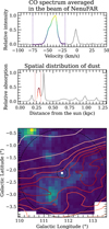 |
Fig. 11 Same as Fig. 10 but for the −47 and −38 km s−1 component of Cas A. |
| In the text | |
|
Fig. 12 Cloud identification for the 3.5 km s−1 component towards Cyg A. Both panels are an overplot of the dust distribution in gray (Edenhofer et al. 2024) and theoretical LSR velocities in blue and red contours (Reid et al. 2019). The largest beam of NenuFAR is marked in black dotted lines. The Sun is represented by the black cross. Top panel: overview of the sightline up to 1.25 kpc from the Sun. The gray contours correspond to the most prominent clouds in the beam of NenuFAR. Bottom panel: zoom on the close vicinity, up to 200 pc from the Sun. The purple cloud crosses the beam towards Cyg A at the expected velocity of 3.5 km s−1. |
| In the text | |
|
Fig. 13 Frequency dependence of beam sizes for NenuFAR and LOFAR, shown alongside the angular size of Cas A. The LOFAR beam is represented for the two CRRLs experiment: Salas et al. (2017) (circles) and Oonk et al. (2017) (squares). Oonk et al. (2017) cropped the images from LOFAR in squares whose sizes are fixed in two frequency windows. Salas et al. (2017) cropped the images from LOFAR in circles centred on Cas A, with continuous values for its diameter. The Nenu-FAR beam size function is shown with the solid line. The red dotted line represents the angular extension of Cas A at radio frequencies (Green 2014). The source is spatially resolved for neither setups, at any frequency. |
| In the text | |
|
Fig. 14 Ratio of the line intensities towards Cas A between observations with NenuFAR and with LOFAR as a function of beam ratio. The crosses represent the filling factor ratios for Cas A and the dots represent the ratio of angular resolutions for the two experiments. If at a given frequency a dot and a cross are close to each other, then the filling factors are similar for both instruments, meaning a less prominent dilution effect between both experiments. The colour scale indicates the central frequency of the lines. The ratio of the line intensities follows the tendency of being farther from one at lower frequencies. The differences in filling factor follow the same tendency. |
| In the text | |
|
Fig. 16 Illustration of the influence of the parameters ne and L on the optimal value found for Te, for Cygnus A. The purple histogram represents all the values of Te that give |
| In the text | |
|
Fig. C.1 Every stack of lines detected towards Cassiopeia A used to extract physical parameters. The coloured lines are the results of the Voigt profile fitting algorithm. The blue lines correspond to the component at –47 km s−1, the green lines are the –38 km.s-1 component and the red lines are the 0 km s−1. The measured line properties can be found in Table C.3. |
| In the text | |
|
Fig. C.2 Every stack of lines detected towards Cygnus A used to extract physical parameters. The purple lines are the results of the Voigt profile fitting algorithm. |
| In the text | |
|
Fig. D.1 Summary of the grid search for Cassiopeia A, component −47 km s−1. The top panel is the histogram of all the nodes of the final grid. The blue part of the histogram highlights the 30% of χ2 that are kept to evaluate the uncertainties. The bottom panels represent for each parameter the values that gives a χ2 distance comprised in the 30% range. |
| In the text | |
|
Fig. D.2 Summary of the grid search for Cassiopeia A, component −38 km s−1. The green part of the histogram highlights the 30% ofχ2 that are kept to evaluate the uncertainties. The bottom panels represent for each parameter the values that gives a χ2 distance comprised in the 30% range. |
| In the text | |
|
Fig. D.3 Summary of the grid search for Cassiopeia A, component −47 km s−1. The red part of the histogram highlights the 30% of χ2 that are kept to evaluate the uncertainties. The bottom panels represent for each parameter the values that gives a χ2 distance comprised in the 30% range. |
| In the text | |
|
Fig. D.4 Summary of the grid search for Cygnus A, component 3.5 km s−1. The purple part of the histogram highlights the 30% of χ2 that are kept to evaluate the uncertainties. The bottom panels represent for each parameter the values that gives a χ2 distance comprised in the 30% range. |
| In the text | |
Current usage metrics show cumulative count of Article Views (full-text article views including HTML views, PDF and ePub downloads, according to the available data) and Abstracts Views on Vision4Press platform.
Data correspond to usage on the plateform after 2015. The current usage metrics is available 48-96 hours after online publication and is updated daily on week days.
Initial download of the metrics may take a while.