| Issue |
A&A
Volume 703, November 2025
|
|
|---|---|---|
| Article Number | A208 | |
| Number of page(s) | 27 | |
| Section | Extragalactic astronomy | |
| DOI | https://doi.org/10.1051/0004-6361/202554843 | |
| Published online | 21 November 2025 | |
MARTA: Temperature-temperature relationships and strong-line metallicity calibrations from multiple auroral-line detections at cosmic noon
1
Università di Firenze, Dipartimento di Fisica e Astronomia, Via G. Sansone 1, 50019 Sesto Fiorentino, Florence, Italy
2
INAF – Arcetri Astrophysical Observatory, Largo E. Fermi 5, I-50125 Florence, Italy
3
European Southern Observatory, Karl-Schwarzschild Straße 2, D-85748 Garching bei, München, Germany
4
Department of Physics, University of Arkansas, 226 Physics Building, 825 West Dickson Street, Fayetteville, AR 72701, USA
5
Scuola Normale Superiore, Piazza dei Cavalieri 7, I-56126 Pisa, Italy
6
Institute for Astronomy, University of Edinburgh, Royal Observatory, Edinburgh EH9 3HJ, UK
7
Centre for Astrophysics Research, Department of Physics, Astronomy and Mathematics, University of Hertfordshire, Hatfield AL10 9AB, UK
8
AURA for European Space Agency, Space Telescope Science Institute, 3700 San Martin Drive, Baltimore, MD 21210, USA
9
Cavendish Laboratory, University of Cambridge, 19 JJ Thomson Avenue, Cambridge CB3 0HE, UK
10
Kavli Institute for Cosmology, University of Cambridge, Madingley Road, Cambridge CB30HA, UK
11
University of Trento, Via Sommarive 14, I-38123 Trento, Italy
⋆ Corresponding author.
Received:
28
March
2025
Accepted:
20
September
2025
Abstract
We present the first results from MARTA (Measuring Abundances at high Redshift with the Te Approach), a programme that leverages ultra-deep, medium-resolution JWST/NIRSpec spectroscopy to probe the interstellar medium of star-forming galaxies at z ∼ 2 − 3. We report detections of one or more auroral lines, including [O III] λ4363, [O II] λλ7320, 7330, [S II] λ4068, and [S III] λ6312, for 16 galaxies in the sample, providing measurements of multiple ionic temperatures. We tested the validity of the T[O II]–T[O III] relation at high redshifts considering a total sample of 21 objects, including literature data, and obtained a shallower slope than in the low-z literature. However, such a slope is consistent with low-redshift data when ultra-low-metallicity objects are considered. We assessed the correlation of the T[O II]–T[O III] relationship and its scatter on different physical parameters, finding a mild correlation with the ionisation parameter and radiation field hardness, and no significant correlation with gas density. The location of high-redshift data is also consistent with the low-z literature in the T[O II]–T[S II] and T[S III]–T[O III] relations, although this conclusion is limited due to low-number statistics. Finally, we leveraged our sample together with a comprehensive compilation of galaxies with [O III] λ4363 detections from the literature to recalibrate classical strong-line diagnostics at high redshifts. MARTA represents a key addition in this space because it provides direct metallicities at moderately high oxygen abundances (12 + log(O/H) ∼ 8.0−8.4).
Key words: galaxies: abundances / galaxies: evolution / galaxies: high-redshift / galaxies: ISM
© The Authors 2025
 Open Access article, published by EDP Sciences, under the terms of the Creative Commons Attribution License (https://creativecommons.org/licenses/by/4.0), which permits unrestricted use, distribution, and reproduction in any medium, provided the original work is properly cited.
This article is published in open access under the Subscribe to Open model. This email address is being protected from spambots. You need JavaScript enabled to view it. to support open access publication.
1. Introduction
Nebular emission from star-forming regions is a fundamental window into the physical conditions and ionising sources within galaxies across cosmic time. For instance, hydrogen recombination lines provide measurements of the star formation rate (SFR) and dust attenuation (Kennicutt 1998; Osterbrock & Ferland 2006; Kennicutt & Evans 2012), while ratios of collisionally excited lines (CELs) from elements like oxygen, nitrogen, and sulphur are sensitive to the electron temperature (Te), electron density (ne), and ionisation state of the gas, enabling the derivation of key physical properties of the ionised gas, including its metal content (Osterbrock & Ferland 2006).
The measurement of chemical abundances in galaxies is a cornerstone of modern astrophysics, offering crucial insights into nucleosynthesis, the history of star formation, and the exchange of gas between galaxies and their surrounding environment (Maiolino & Mannucci 2019; Kewley et al. 2019). In extragalactic astrophysics, the ‘gold standard’ approach to determining the metallicity of the interstellar medium (ISM) involves deriving electron temperatures from faint auroral lines (Peimbert 1967; Stasińska 2002). In particular, ratios of auroral to nebular CELs are exponentially sensitive to the electron temperature as auroral lines originate from higher energy levels compared to nebular ones (Peimbert 1967; Osterbrock & Ferland 2006; Peimbert et al. 2017).
For the purposes of inferring abundances, H II regions are generally modelled using a two-zone model consisting of a low- and a high-ionisation zone. Of the optical lines, the auroral [O III] λ4363 line has frequently been used infer oxygen electron temperatures of the high-ionisation zone and consequently the abundance of O++. Measurements of the total oxygen abundance, however, require the detection of multiple auroral lines from both low- and high-ionisation species to accurately constrain electron temperatures throughout the nebula (e.g. Pilyugin 2007; Andrews & Martini 2013; Berg et al. 2015; Curti et al. 2017). Alternatively, a relation between the temperatures of the different ionisation zones (temperature-temperature, or T − T relation) can be adopted (e.g. Campbell et al. 1986; Garnett 1992; Pilyugin et al. 2009; Méndez-Delgado et al. 2023a).
A fundamental limitation to measuring chemical abundances using auroral lines is that they are often significantly fainter than the corresponding strong nebular lines (by tens to even hundreds of times, especially at high metallicities) since their excitation requires higher-energy electrons (Kennicutt et al. 2003; Esteban et al. 2004; Berg et al. 2020). Empirical metallicity calibrators, based on strong line ratios such as [N II] λ6584/Hα, [O III] λ5007/Hβ, [O III] λ5007/[O II] λλ3727,3729, or [O III] λ5007/[N II] λ6584, offer an alternative approach by utilising only strong nebular emission lines (e.g. Pettini & Pagel 2004; Curti et al. 2017; see Maiolino & Mannucci 2019 for a review). However, such calibrators are subject to significant limitations as strong-line ratios depend not only on metallicity but also on other parameters, such as the gas density, ionisation parameter, hardness of the ionising spectrum, and relative element abundances (Garnett 2002; Mollá et al. 2006; Pérez-Montero & Contini 2009; Kewley et al. 2019).
Moreover, empirical calibrations established for local galaxies are not directly applicable to high-redshift galaxies. Extensive observational evidence has demonstrated that galaxies atz ∼ 2 exhibit harder ionising spectra – likely driven by α enhancements in high-redshift star-forming galaxies (Steidel et al. 2016; Topping et al. 2020; Cullen et al. 2021; Stanton et al. 2024) – and higher electron densities compared to their z ∼ 0 counterparts (Erb et al. 2006; Hainline et al. 2009; Bian et al. 2010; Yabe et al. 2012; Tacconi et al. 2013; Kewley et al. 2013; Masters et al. 2014; Nakajima & Ouchi 2014; Sanders et al. 2016; Shapley et al. 2019; Topping et al. 2025a). These differences are reflected in diagnostic diagrams such as the N2-BPT (Baldwin, Phillips & Terlevich; Baldwin et al. 1981) diagram, log([O III]/Hβ) versus log([N II]/Hα), where high-redshift galaxies are systematically offset from their local counterparts (Steidel et al. 2014; Masters et al. 2014, 2016; Shapley et al. 2015; Strom et al. 2018; Topping et al. 2020). Strong-line ratios like [N II]/Hα and [O III]/Hβ become increasingly influenced by other physical parameters at higher redshifts, such as the shape of the ionising spectrum and the ionisation parameter. As a result, their reliability as metallicity tracers is compromised, leading to potential biases when applied to high-redshift galaxies (Bian et al. 2018; Sanders et al. 2021).
The ideal solution is to measure metallicities directly using auroral lines sensitive to electron temperatures, bypassing the uncertainties inherent to empirical calibrators. In cases where only a single auroral line is available, locally calibrated relations (e.g. between the temperature of O+ and O++, known as T2 − T3 relations) must be assumed, a situation that introduces additional uncertainties. Detecting these faint lines in individual high-redshift galaxies was extremely challenging prior to JWST, with only a few, low-significance detections of [O III] λ4363 reported at z > 2 (e.g. Christensen et al. 2012; James et al. 2014; Sanders et al. 2020; see also the compilation by Patrício et al. 2018) and rare cases of auroral [O II] λλ7320, 7330 detections, such as those presented in Sanders et al. (2023) for two galaxies at z > 2. This scarcity hindered the accurate determination of metallicities in distant galaxies, necessitating the use of empirical metallicity indicators calibrated on lower-redshift systems.
The JWST Near Infrared Spectrograph (NIRSpec; Jakobsen et al. 2022), with its unparalleled sensitivity and wide spectroscopic wavelength coverage of the near-infrared regime, has revolutionised this field, enabling the detection of auroral lines in galaxies both at cosmic noon (z ∼ 2 − 3; e.g. Strom et al. 2023; Welch et al. 2024, 2025; Rogers et al. 2024) and at much higher redshifts (Curti et al. 2023; Yang et al. 2023; Laseter et al. 2024; Morishita et al. 2024a; Sanders et al. 2024; Arellano-Córdova et al. 2025; Cullen et al. 2025; Scholte et al. 2025; Shapley et al. 2025; Stanton et al. 2025). These efforts have delivered some of the most accurate determinations of gas-phase abundances in early galaxies. Interestingly, the higher sensitivity of JWST/NIRSpec towards the redder part of the spectrum, combined with the metal deficiency, higher ionisation conditions, and compact nature of high-z systems, as well as the tendency of most JWST programmes to focus on the high-z Universe, has made auroral line detections more likely at very high z than at z ∼ 2 − 3, where galaxies are typically more massive, extended, and metal-rich than at z ≳ 5. Moreover, very few observations have enabled detections of multiple auroral lines, which are necessary to probe the temperature and ionisation structure of high-redshift galaxies.
While this paper was under review, an independent analysis by Sanders et al. (2025) presented results from the AURORA (Assembly of Ultradeep Rest-optical Observations Revealing Astrophysics) survey, combining new JWST/NIRSpec observations with literature data to investigate temperature–temperature relations and to calibrate strong-line metallicity diagnostics at z ∼ 2 − 10. They found that local T2 − T3 relations remain valid at high redshifts, while empirical strong-line calibrations show clear offsets with respect to the local ones, consistent with evolving ISM conditions; in particular, diagnostics based on α elements provide the most reliable metallicity estimates, whereas nitrogen-based indicators exhibit significant scatter, likely due to variations in N/O at fixed O/H.
In this paper we present novel observations of multiple auroral lines in spectra of individual galaxies at cosmic noon from the MARTA (Measuring Abundances at high Redshift with the Te Approach) survey (PID 1879, PI Curti), which targeted 127 galaxies in the COSMOS (Cosmic Evolution Survey) field at redshifts z ∼ 2 − 3 by means of very deep NIRSpec Micro Shutter Array (MSA) observations. In Curti et al. (2025a), the multiple science cases addressed by such a programme are discussed, with a focus on the ISM properties and chemical abundances of one of the galaxies in the sample.
Here, we leveraged a sample of 16 galaxies with (multiple) detections of auroral lines, mainly [O III] λ4363 and [O II] λ7320,7330 but also [S II] λ4069 and [S III] λ6312. This sample extends the parameter space probed by cosmic noon galaxies with auroral line detections towards higher metallicities than most existing studies. We focus on the relationships between temperatures inferred from different ionic species and their possible redshift evolution. We discuss the implications for the applicability of the Te method for measuring metallicity in high-z galaxies and investigate the redshift evolution of some of the most widely adopted strong-line metallicity diagnostics.
The paper is structured as follows. Section 2 outlines the survey design, including the target selection, observational strategy, and data reduction process. In Sect. 3 we detail the data analysis methodology and the spectral fitting procedure. Section 4 defines the two subsamples of the MARTA survey, golden and silver, which are used for all subsequent analyses. In Sect. 5 we describe the dust correction procedure applied. Section 6 focuses on the oxygen temperature-temperature relation, the analysis of their dependence on other parameters such as density and the ionisation parameter, and a comparison with sulphur temperatures. Section 7 presents the results on strong-line calibrations. Finally, in Sect. 8 we provide a summary of our conclusions and prospects for future research.
In this work we use the following notation to refer to the strong-line diagnostics:
-
R3 = log ([O III] λ5007/Hβ)
-
R2 = log ([O II] λ3726,3729/Hβ)
-
O32 = R3 − R2
-
R23 = log [([O II] λ3726,3729 + [O III] λ4959,5007)/Hβ]
-
 = 0.46 R2 + 0.88 R3
 -
Ne3O2 = log ([Ne III] λ3869/[O II] λ3726,29)
-
N2 = log ([N II] λ6585/Hα)
-
O3N2 = R3 − N2
-
S2 = log [([S II] λ6716 + [S II] λ6730)/Hα]
-
O3S2 = R3 − S2
2. Observations and data reduction
2.1. Target selection, priority classes, and observing strategy
The MARTA programme focuses on the redshift range around the peak of cosmic star-formation activity (cosmic noon), with the primary aim to detect the auroral lines of [O III] λ4363 in the G140M (R ∼ 1000) grating and, for a subsample, the [O II] λ7320,7330 lines in the G235M (R ∼ 1000) grating. Considering the need to cover [O II] λλ3727,29 to measure electron temperatures and derive metallicities, this constrains the primary redshift range of our targets to 1.7 < z < 3.1. However, a few higher-redshift sources were also observed, according to selection and prioritisation criteria described below.
The MARTA parent catalogue was generated from the COSMOS2020 (Weaver et al. 2022) and the 3D-HST (3D Hubble Space Telescope) catalogues (Skelton et al. 2014; Momcheva et al. 2016) based on a multi-step process. The COSMOS2020 catalogue provided photometric redshifts while the 3D-HST catalogue provided grism spectroscopic redshift data, which were complemented by spectroscopic redshifts from higher spectral resolution, ground-based observationsavailable at the time of MSA mask design (including zCOSMOS-bright, Lilly et al. 2009; FMOS, Silverman et al. 2015; MOSDEF, Kriek et al. 2015; zFIRE, Nanayakkara et al. 2016; VUDS, Tasca et al. 2017; hCOSMOS, Damjanov et al. 2018; DEIMOS 10k, Hasinger et al. 2018; LEGA-C, Straatman et al. 2018; KMOS3D, Schreiber et al. 2019; KLEVER, Curti et al. 2020a; and data from Kartaltepe et al. 2010, 2015; Masters et al. 2012; Balogh et al. 2014; Comparat et al. 2015; Schreiber et al. 2018). When ground-based spectroscopic redshifts were not available, lower resolution, grism-based redshifts were adopted. In the absence of both, photometric redshifts were used, provided they were consistent between LEPHARE (Ilbert et al. 2006) and EAZY (Brammer et al. 2008), within a defined tolerance (Δ(z)/z < 0.1, considering the redshift estimates from EAZY).
For each galaxy in the MARTA parent catalogue, we estimated the expected flux of the [O III]λ4363 emission line based on the available information on stellar masses (M⋆), SFR, and metallicity, as described in the following. The stellar masses, SFR, and dust attenuation (AV) were adopted from spectral energy distribution fitting of the photometry extracted by COSMOS2020 (Weaver et al. 2022). When ground-based spectroscopy (either slit or integral field unit) in COSMOS covering Hα was available, as provided by, for example, the KMOS3D (K-band Multi Object Spectrograph 3D survey) (Wisnioski et al. 2019), KLEVER (KMOS Lensed Emission-Line Velocity and Metallicity Survey, Curti et al. 2020a), and MOSDEF (MOSFIRE Deep Evolution Field survey, Kriek et al. 2015) surveys, the SFR was estimated from the extinction-corrected Hα flux using the relation from Kennicutt & Evans (2012) and the AV derived from either photometry or from the Balmer decrements. As of gas-phase metallicity, we assumed the value for oxygen abundance derived from strong-line diagnostics and the Bian et al. (2018) calibrations, specifically those based on local analogues of high-redshift galaxies, for galaxies with available spectroscopy and detection of at least three nebular emission lines, whereas we estimated the expected metallicity for each source with no previously available spectra assuming that the relationship between metallicity, mass, and SFR (so-called fundamental metallicity relation; Mannucci et al. 2010) does not evolve with redshift up to z ∼ 2 (Cresci et al. 2019; Sanders et al. 2021), adopting specifically the parametrisation of Curti et al. (2020b).
Finally, we based our indirect estimate of the [O III]λ4363 flux on the relationship between the [O III]λ4363/Hα ratio and metallicity, the latter calibrated on a combined sample of local H II regions and low-metallicity galaxies from Guseva et al. (2011), Berg et al. (2020), and stacks from SDSS (Sloan Digital Sky Survey, Curti et al. 2017) with ‘direct’, Te-based oxygen abundances. Such intrinsic [O III]λ4363 flux was then attenuated by the galaxy AV, assuming the attenuation curve of Cardelli et al. (1989) and an RV = 3.1, to derive our final estimate of the expected [O III]λ4363 flux in each source.
Galaxies in the MARTA parent catalogue were assigned to four different priority classes (each one with different weights) to drive the MSA target allocation. Such classes were established on the basis of the expected emission line fluxes (estimated as detailed above), while additional factors such as dust attenuation and redshift reliability were also considered to fine-tune the weights assignment and optimise the final MSA mask. The detailed list of the criteria assumed in target prioritisation is reported in Table 1. A total of 126 sources, including 18 ‘priority one’, 22 ‘priority two’, 12 ‘priority three’, 21 ‘priority four’, targets and 53 ‘filler’ sources, were observed using a single MSA configuration, though only galaxies belonging to the top two classes were used to drive the choice of the pointing coordinates.
Target prioritisation criteria.
Each galaxy was observed through a three-shutter slitlet, and observations were taken adopting a standard nodding strategy with three nod positions along the slitlet. To maximise the number of targets observable within a single pointing, we allowed spectral traces to overlap on the detector, as the probability of overlapping emission lines from two different sources was estimated to be minimal. However, due to the depth of our observations, significant continuum emission was detected in many cases. The impact of this observing choice on background subtraction is discussed in Sect. 2.2.
Observations were obtained totalling an integration time of 31.9 hours in G140M, 7.4 hours in G235M, and 2.9 hours in G235H. The G235H is intended for studies of emission-line kinematics and is therefore not used in this work, where we instead focused on the G140M and G235M data.
2.2. Data reduction
The data reduction of our observations was performed using the JWST calibration pipeline, which is divided into three stages. We applied the pipeline version ‘2023_2a’ and CRDS (Calibration Reference Data System) context files ‘jwst_1183.pmap’. Stage 1 applies detector-level corrections, including group-by-group corrections and ramp fitting, producing a count rate image for each exposure. Stage 2 focuses on instrument-specific and observing-mode calibrations, resulting in fully calibrated individual exposures. At this stage, the standard nodding background subtraction is performed, and path-loss corrections estimated for point-like sources are applied.
Stage 3 combines multiple exposures, such as those from nodding and dither patterns, into a single 2D spectral product, while applying outlier rejection and additional corrections as needed. Although the pipeline also provides a final extracted 1D spectrum, we performed a bespoke extraction of 1D spectra for each target as described later in this section. Other parameters in the data reduction pipeline were kept to their default values.
Due to our observing strategy (allowing spectral overlap) and the spatially extended nature of our sources, in several cases a dedicated background subtraction is required. In particular, our data suffer from spectral contamination from sources located in different MSA slits, whose continuum emission could contaminate the central shutter of the slitlet and/or the flanking ‘background’ shutters. Moreover, in some cases, the flux from the target object is extended or not well centred, and extends into the micro-shutters adjacent to the central one. As a result, applying the standard nodding background subtraction, which subtracts the background pixel-per-pixel using the same shutter after offsetting (Fig. 1, left), can lead to over-subtraction of the target’s flux and/or to a poor modelling of the background itself.
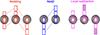 |
Fig. 1. Comparison of strategies for background subtraction in NIRSpec/MSA observations. Left (red): Standard three-point nodding strategy, in which the galaxy is observed in three positions within the shutter, and the background for each position is estimated using the corresponding shutter exposures from the other two nods. Centre (blue): Nod2 strategy, a two-position scheme where only two out of the three available positions are used for the nodding procedure in order to use the shutters farthest from the galaxy as the background. Right (magenta): Local subtraction approach, which uses the outer shutters from the two off-source positions (indicated by the filled-in shutters) to estimate the sky background. In this method, the object signal is taken from the sum of all three nod positions (connected by dashed magenta lines), but no background is subtracted from the same shutters. As such, this method can be more sensitive to local systematics or background gradients. |
To mitigate over-subtraction in cases of extended sources, we calculated the expected contamination of the flanking shutters by the source flux using NIRCAM (Near InfraRed Camera) imaging data from the PRIMER (PRism and Imager for Extragalactic Research) survey (PID:1837, Dunlop et al. 2021) in bands F115W, F150W, F200W, and F277W (broadly corresponding to the wavelength range probed by our NIRSpec observations in G140M and G235M). The reduced and calibrated NIRCam imaging data products were retrieved from the Dawn JWST Archive (DJA1).
For galaxies where PRIMER imaging and 2D spectra indicate that the emission is visibly extended beyond the central shutter, we adopted a so-called ‘nod2 subtraction’ strategy (e.g. Maseda et al. 2024). In this approach, only two of the nods-specifically, the ones where the galaxy is in the outermost shutter-are used. This minimises the risk of self-subtraction, where the galaxy’s emission would be subtracted along with the background, while maintaining the advantage of pixel-by-pixel subtraction, which mitigates detector artefacts. However, this strategy comes at the cost of sacrificing one-third of the total exposure time, as the exposure in which the galaxy is located in the central shutter is excluded (Fig. 1, middle).
An alternative approach to background subtraction consist in employing the combined, non-background subtracted 2D spectra from all three nodded exposures to extract and construct a ‘local’ background as the average of the two outermost shutters. Specifically, we extracted the background spectrum from the two outermost shutters in the nodding configuration, summing the flux across all pixels in each shutter and then averaging the results to obtain a representative background spectrum (Fig. 1, right). The galaxy spectrum was extracted from a boxcar aperture centred on the peak of the S/N in the spectral trace of the target and of width of 5 pixels (roughly equivalent to the size of one shutter), although in some cases extended line emission as visible in the 2D spectra suggested to increase the size of the extraction aperture to avoid significant flux losses and possible biases in the inferred line ratios. Such a ‘local subtraction’ strategy benefits from the full on-source integration time by co-adding all three nodded exposures but suffers from the increased noise affecting the background spectrum, which is generated from exposures with shorter effective integration times than the central trace containing the target source. Moreover this strategy does not leverage the pixel-by-pixel background subtraction of the standard ‘nodding’ therefore sometimes resulting in spectra with worse noise properties due to detector artefacts. For compact galaxies or those that do not show significant emission in adjacent shutters, the standard nodding background subtraction was applied and we checked that the fluxes obtained from the local background subtraction are comparable. Specifically, we applied the local background subtraction for galaxy MARTA_3942, the nod2 method for MARTA_4195, and the standard nodding background subtraction for the remaining sources. To compare the results of these different strategies and ensure that absence of self-subtraction, we assessed their impact on the extracted and measured fluxes of [O III] λ5007 in the G140M and on the Hα in the G235M gratings, respectively. We verified that, had the standard nodding procedure been used in the case of extended galaxies, these lines would have been significantly underestimated. In particular, we tested the effect on MARTA_3942 and MARTA_4195, and found that the [O III] flux is affected by 13−22% and the Hα flux by 7−20%.
As some of our galaxies look morphologically extended, they might be affected by larger slit losses than modelled for simple point-like sources. On the other hand, in several cases the bulk of the emission captured by the slit comes from bright individual clumps, and hence the assumption of constant surface brightness across the slit is also incorrect. The analysis presented in this work only relies on emission lines ratios, and is therefore not affected by uncertainties on the absolute flux calibration. However, a second-order correction to the relative line fluxes is expected due to the point-spread-function dependence of the path-loss correction, which is not modelled here. To test the reliability of the relative flux calibration in our spectra, we measured the ‘intra-shutter’ photometry from NIRCam imaging in the F115W, F150W, F200W, and F270W broadband filters (sampling the spectral range covered by G140M and G235M gratings), compared it to the synthetic photometry extracted by applying the transmission curve of each filter to the spectra, and verified that for the 16 galaxies analysed in the present study no significant relative flux calibration mismatch between the blue-end and red-end part of each grating was observed.
Finally, we verified the consistency of the relative flux calibration across gratings by analysing the overlapping region between G140M and G235M spectra, which roughly spans the 1.66 and 1.90 μm wavelength interval. Specifically, we calculated the ratio of continuum fluxes between the G140M and G235M gratings for seven galaxies in our sample (Sect. 4.2). For most galaxies, these ratios fell within 5% of unity – i.e. between 0.95 and 1.05 – demonstrating excellent agreement between the two gratings. For galaxies with ratios outside this range, the discrepancies were attributable to contaminants in the bluest or reddest regions of the spectra, as evident by inspecting their 2D spectra. We therefore did not perform a correction to the flux calibration of the gratings.
3. Spectral fitting
We measured spectroscopic redshifts for 73 out of the 126 targets by using strong lines, such as [O III] λ5007 and Hα. A detailed description of the spectral properties for the full sample will be presented in a future publication.
We performed spectral fitting on the 1D data using the PYTHON module of the penalised pixel-fitting (PPXF) routine (Cappellari & Emsellem 2004), which can simultaneously fit both galaxy emission lines and the underlying stellar continuum. Since the emission lines are not spectrally resolved, we modelled them using a single Gaussian component per line. The emission lines included in our analysis are listed in Table E.1. For the continuum fitting, we used eMILES stellar population templates (Vazdekis et al. 2016, 2010) with BaSTI isochrones (Pietrinferni et al. 2004) and a Chabrier (2003) initial mass function. We modelled the line spread function with a Gaussian profile varying as a function of wavelength, using the spectral resolution profiles provided in the JWST documentation for the G140M and G235M filters2.
We assessed the impact of different stellar population libraries by systematically comparing the measured fluxes of key emission lines, focusing in particular on [O III] λ4363. Although the strength of Balmer absorption features varies noticeably across templates, the effect on the [O III] λ4363 flux remains minor – typically less than ∼10%, with a median variation of ∼6%. A more detailed description of these tests is provided in Appendix B.
A 24-degree multiplicative polynomial was applied to modify the continuum templates, accounting for potential dust reddening, residual flux calibration uncertainties, and template mismatch effects. The choice of polynomial degree was determined through a systematic analysis comparing different orders (5, 10, and 24) by evaluating the quality of the fit and the statistical properties of the residuals, with specific focus on the line-free region between rest-frame 4125 and 4325 Å, chosen to assess the goodness of the fit in proximity to the auroral [O III] λ4363 line. The 24-degree polynomial consistently yielded the best results, indicating an improved match between the model and the observed spectrum. Nonetheless, we verified that the variations in the emission lines driven by the choice of different polynomial degrees do not significantly impact the results presented in this work. Further discussion of the impact of the continuum subtraction on the measurement of weak auroral lines and an example spectral fit is presented in Sect. 4.2. Within each grating, the velocity (v) and velocity dispersion (σ) parameters of the various emission lines were tied together, forcing a consistent kinematic structure for the emission regions. We performed the fitting separately for each of the two gratings, G140M and G235M. Where emission lines were serendipitously observed in both gratings, their fluxes are consistently in agreement within the uncertainties.
4. Auroral emission lines in the MARTA sample
4.1. Properties of galaxies with auroral line detections
In this work we focused on a subset of 16 galaxies with one or more auroral line detections. We note that this subsample has been explicitly selected and prioritised on the basis of the likelihood of [O III] λ4363 detection. As a consequence, it could be biased towards galaxies with elevated auroral [O III] fluxes, which in turn correspond to higher electron temperatures, lower metallicities, and higher SFRs. This selection effect must be kept in mind when interpreting the physical properties of these galaxies in a broader context. However, as we show later in this section, strong-line diagnostic analyses do not reveal significant systematic biases. Nonetheless, potential biases could emerge in scaling relations, which are beyond the scope of this paper but should be carefully considered in future studies.
We classified these 16 galaxies into two groups: we considered the seven galaxies with both [O III] λ4363 and [O II] λ7320,7330 detections as our ‘golden sample’ and the remaining nine galaxies with detections of [O III] λ4363 only as the ‘silver sample’. For five galaxies in the golden sample, additional auroral lines from both high-ionisation and low-ionisation ions are detected.
Figure 2 shows the distribution of all observed MARTA targets (marked according to their different priority classes) in the M⋆–SFR plane. The parametrisation of the star-forming main sequence (SFMS; Noeske et al. 2007) at z = 2.15 (median redshift of the sample) from Popesso et al. (2023) is also shown for comparison. Galaxies with with auroral lines detections in MARTA sit preferentially above the SFMS at z = 2.15, having SFRs between 5 and 30 times higher the average at fixed M⋆.
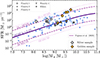 |
Fig. 2. Star formation main sequence for the MARTA sample. Different shapes correspond to different priority classes, as described in Table 1, and different colours to the different samples: the golden sample is in orange (Sect. 4.2), the silver sample in grey (Sect. 4.3), and the rest of the galaxies in blue. For comparison, we plot the parametrisation of the star-forming main sequence at z ∼ 2.15 (median redshift of the full MARTA sample) by Popesso et al. (2023). |
In Fig. 3 we plot the position of the MARTA galaxies analysed in the present study (the golden and silver samples) onto different emission line-based diagnostic diagrams, namely R23 versus O32, the [N II]-BPT diagram, and the [S II]-BPT ([S II]/Hα vs [O III]/Hβ). In the R23 versus O32 diagram MARTA galaxies at z > 3 are offset from both the SDSS and MOSDEF (z ∼ 2 − 3, Kriek et al. 2015) contours, occupying a region generally associated with high-ionisation, low-metallicity systems, as recently probed by large (though shallower) JWST surveys such as JADES (JWST Advanced Deep Extragalactic Survey) (Cameron et al. 2023a) and CEERS (Cosmic Evolution Early Release Science Survey) (Sanders et al. 2023). In the BPT diagrams, MARTA galaxies at z ∼ 2 occupy the upper envelope of the local SDSS distribution, showcasing also the known offset in the [N II]-BPT, (Steidel et al. 2014; Shapley et al. 2015). They overlap with the regions populated by surveys targeting z ∼ 2 − 3 galaxies, such as MOSDEF and KBSS (Keck Baryonic Structure Survey) (Strom et al. 2017).
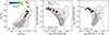 |
Fig. 3. Diagnostic diagrams for the MARTA galaxies analysed in this work. From left to right: Distribution of the combined golden and silver samples on the O32 vs R23, [O III]/Hβ vs [N II]/Hα, and [O III]/Hβ vs [S II]/Hα diagrams, colour-coded by galaxy redshift. The grey contours indicate the region populated by local galaxies from SDSS, with darker shades denoting higher densities. Red contours mark the distribution of galaxies from the MOSDEF survey (Kriek et al. 2015), whereas the orange curve is the fit to KBSS galaxies from Strom et al. (2017); both surveys target primarily z ∼ 2 − 3 systems. The dividing lines between star-forming galaxies, AGNs, and LINER galaxies from Kewley et al. (2001, 2013) and Kauffmann et al. (2003) in both the [N II]-BPT and [S II]-BPT diagrams are also drawn. Median error bars are not shown, as they are smaller than the symbol size and would not be visible in the plot; this is due to the fact that these are among the strongest lines, measured with very high S/Ns. |
Based on classical classification schemes, such as those provided by Kewley et al. (2001, 2013), Kauffmann et al. (2003), we find no evidence of active galactic nucleus (AGN) contamination. This conclusion is corroborated also by the absence of specific AGN spectral features in our sample, such as broad components in the Balmer emission lines, very high-ionisation species, or He II emission3. Furthermore, as described in Sect. 6, we do not find unusually high (≳25 000 K) electron temperatures that could be associated with AGN ionisation (e.g. Mazzolari et al. 2024).
4.2. The MARTA golden sample: Multiple auroral line detections
The MARTA golden sample consists of seven galaxies with S/N ≳ 5 detections of the [O III] λ4363 auroral line and S/N ≳ 3 for the [O II] λλ7320,7330 auroral doublet (where each line in the doublet is detected at ≳3σ). The S/N on emission lines was estimated from both the output of the PPXF fitting and the RMS of the spectra within a featureless region around the emission line of interest; a comparison between these two methods is presented in Appendix A. As reported in Table 2, the golden sample spans z = [1.8 − 2.2], log(M*/M⊙) = [9.2 − 9.8] and SFRs ranging from 2.6 to 310 M⊙/yr (with a mean value of 80 M⊙/yr). These galaxies lie on average significantly above the median SFMS at z ∼ 2 (Fig. 2). We quantified the ΔMS as the distance in log(SFR) from the parametrisation of Popesso et al. (2023), and found ΔMS values spanning from −0.2 to +1.3 dex, with a median value of +0.47 dex.
Physical properties of MARTA galaxies in the golden (top) and silver (bottom) samples.
Galaxy MARTA_1084 was excluded from this sample, despite detections of both oxygen auroral lines, because its [O II] λ3726,3729 line falls within the detector gap, precluding its use for O+ electron temperature calculation and thus for direct metallicity determination. We therefore included this galaxy in the silver sample.
For some of these galaxies we also report the detection of additional auroral lines. In particular, the [S II] λ4068 auroral line is detected with S/N > 3 in four cases. Similarly, the [S III] λ6312 auroral line is detected at ≳3σ in three galaxies, where a proper de-blending from the nearby nebular [O II] λ3727 line can be performed. Figure 4 shows a compilation of the auroral line detections across this subsample. Although MARTA_1084 was excluded from the golden sample, it is included in the plot as it displays two auroral lines. In this figure, each panel corresponds to one of the auroral emission lines, with the continuum-subtracted spectrum shown along with the fitted Gaussian model. In some cases bespoke line fits were performed for individual objects, as detailed in Appendix B.
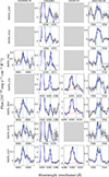 |
Fig. 4. Auroral emission lines detected in the MARTA golden sample. The panels show emission line fits of the [S II] λ4068,4076, [O III] λ4363, [S III] λ6312, and [O II] λ7320,7330 transitions, with their rest-frame wavelengths marked as dashed blue lines. We show the continuum-subtracted spectra in black, and the Gaussian emission-line fits in blue. In the case of [S III] λ6312, two single Gaussians are shown (dashed red lines), since the [S III] line is blended with the [O II] λ6300. |
Figure 5 reports instead the complete spectral fitting, for both G140M and G235M gratings, for one of the galaxies in the golden sample – MARTA_4502. This spectrum is representative of the quality and S/N of other objects in the golden sample. We observe strong continuum with clear stellar absorption features under the Balmer lines. We observe multiple high-S/N auroral lines, including [O II] λλ7320,7330, [O III] λ4363, and [S II] λ4068. The Balmer series is observed up to H10, and generally detected up to H7 in all golden sample galaxies. In several objects, Paschen 10 and Paschen 11 are also visible. We note the presence of other semi-strong emission lines, such as [Ne III] and [S III] λλ9071,9533, which are particularly valuable as they provide insights into the chemical abundances and ionisation level of the elements in the gas, enabling more detailed studies of chemical abundance patterns (e.g. Stanton et al. 2025).
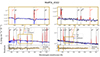 |
Fig. 5. Spectral fit for MARTA_4502, observed using grating G140M (left) and G235M (right). The black line represents the observed flux, the blue line the stellar continuum fit, and the red lines the emission-line Gaussian fits. In the bottom panels we show in grey the residuals from the fit, while the orange line represents the pipeline error estimates. The zoom-in panels at the top provide a more detailed view of specific spectral features: the auroral lines [S II] λ4068 and [O III] λ4363 (left) and the spectral range around the [O II] λλ7320,7330 auroral lines (right). |
4.3. The MARTA silver sample: Single auroral line detections
The MARTA silver sample consists of nine galaxies, including eight additional detections of the auroral [O III] λ4363 line with S/N > 5 (Table 2). Additionally, we included the previously discussed MARTA_1084 in this sample. In Fig. 6 we show a zoom-in of the spectral region around the [O III]λ4363 auroral line in these systems, with the best-fit model overlaid.
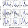 |
Fig. 6. [O III] λ4363 auroral emission line detected in the MARTA silver sample. The continuum-subtracted spectra are shown in black, with Gaussian emission-line fits overlaid in blue. The dashed light blue lines mark the rest-frame wavelength of the [O III]. |
These galaxies span a broader redshift range than the golden sample objects, with two objects at z > 3 and one at z > 4. The silver sample also has generally lower stellar masses, log(M⋆/M⊙) = [8.13 − 9.9], and a ΔMS spanning from −0.66 to +1.2 dex, with a median value of +0.43 dex, so slightly less star-forming, on average, than the golden sample. Although these galaxies cannot be used to evaluate the relationships between the temperatures of different ionic species, they are employed in Sect. 7 to recalibrate the relationships with strong-line diagnostics.
5. Balmer decrements and dust attenuation
To correct the measured emission line fluxes for dust attenuation, we primarily relied on the ratios among the strongest Balmer lines observed in MARTA spectra, namely Hα/Hβ, Hγ/Hβ, and Hδ/Hβ, noting that Hα/Hβ typically involves computing a ratio between lines measured across the G235M and G140M gratings. We employed the Cardelli et al. (1989) extinction curve and computed the E(B − V) utilising the PYNEB routine (Luridiana et al. 2015) assuming intrinsic Balmer line ratios of Hα/Hβ = 2.86, Hγ/Hβ = 0.468, and Hδ/Hβ = 0.259, as predicted by Case B recombination assuming an electron temperature Te = 104 K and electron density ne = 100 cm−3 (Osterbrock & Ferland 2006). To verify the impact of these assumptions, we implemented an iterative procedure in which the extinction correction was recomputed at each step using updated values of Te and ne derived from the previous iteration. This process was repeated until convergence. We found that the resulting changes in E(B − V) and in the derived physical properties are minimal: both Te and ne vary by less than 2% across the entire sample. These small differences confirm that the use of fixed values for the extinction correction does not introduce any significant bias in our analysis.
The E(B − V) was determined by minimising a χ2 function defined by co-adding in quadrature the differences between the three observed Balmer line ratios and their theoretical values, given the adopted reddening curve. The resulting best-fit value was adopted as our fiducial E(B − V) and used to correct all line fluxes. The use of an alternative attenuation curve, such as the Calzetti et al. (1994) law, the Small Magellanic Cloud law (Gordon et al. 2003), or the parametrisation of Reddy et al. (2020) calibrated on z ∼ 1 − 3 galaxies does not significantly affect our results. Reddy et al. (2023) recently analysed galaxies at similar redshifts to our MARTA sample using Paschen line ratios and found a dust attenuation behaviour consistent with that of the Small Magellanic Cloud.
However, the E(B − V) values derived individually from different Balmer line ratios within the same galaxy were not always consistent among themselves, with differences reaching up to 0.3 dex in some cases. We therefore also computed the dispersion among E(B − V) values estimated from Hα/Hβ, Hγ/Hβ, and Hδ/Hβ individually, which we report in Table 2; however, this systematic uncertainty is not propagated throughout the rest of the analysis.
Discrepancies among E(B − V) as derived from different ratios of Balmer lines have been observed before at high redshifts. For instance, McClymont et al. (2025) modelled Balmer decrements in JADES observations at z > 2 by studying the differential impact of radiation- and density-bounded nebulae, showing how, in the latter case, Balmer line ratios deviate from Case B values in a way that could partially explain the observed discrepancies in E(B − V) when different ratios are used. In that scenario, for moderate- to high-metallicity conditions (such as those probed by MARTA galaxies), the Hγ/Hβ ratio is predicted to take higher values than in the case B scenario. Hence, any dust reddening would lower that ratio to closer to the case B theoretical value (mimicking no dust), while increasing Hα/Hβ.
Another possibility to explain such discrepancies involves a different shape of the extinction curve in high-z galaxies. Recent work by Sanders et al. (2025) shows that for a galaxy at z = 4.41, the inferred extinction curve deviates significantly from both the Calzetti et al. (1994) and Cardelli et al. (1989) laws, exhibiting a steeper slope at long wavelengths and a shallower slope in the ultraviolet. This finding suggests that commonly assumed dust laws are not universally applicable to high-redshift galaxies. If a similar effect is present in our sample, the adoption of a different extinction curve could partially account for the discrepancies observed in E(B − V) estimates. A more detailed investigation into the behaviour of E(B − V) and the disagreement between different individual Balmer line ratios is beyond the scope of this work, and will be addressed in future work.
6. The temperature-temperature relations
To determine the chemical composition of a photoionised nebula, one needs to measure (or assume) its temperature and density structure (Stasińska 2002). A commonly adopted approach models the nebula as constituted by two main ionisation zones: a high-ionisation and a low-ionisation zone. In this framework, the electron temperature of the O2+ ion, referred to as T3, characterises highly ionised species. In contrast, the electron temperature of the O+ ion, denoted T2, represents low-ionisation species such as S+ or N+. Some species, such as S2+, have an intermediate ionisation potential between the two zones and may therefore overlap both (e.g. Berg et al. 2020).
In this section we leverage some of the first available measurements of electron temperatures from different ionic species as delivered by JWST (including T2, T3, and, for a subset of targets, the temperatures associated with sulphur ions S+ and S2+) to study temperature-temperature relationships at high redshifts, assess possible evolution from their low-z counterparts, and analyse trends with different physical properties. Throughout this section and the rest of the paper, we have adopted the following atomic parameters and collisional strengths: Palay et al. (2012) for [O III], Kisielius et al. (2009) and Zeippen (1982) for [O II], Rynkun et al. (2019) and Tayal & Zatsarinny (2010) for [S II], Podobedova et al. (2009) and Tayal & Gupta (1999) for [S III], for collisional strength and atomic parameters, respectively.
To estimate the uncertainties on the computed properties, we randomly perturbed the best-fit line fluxes by adding noise sampled from a Gaussian distribution with sigma equal to the flux uncertainties, and derived the corresponding electron temperature and density 100 times. The fiducial values and associated uncertainties of these quantities were then quantified as the mean and standard deviation of the distributions obtained, respectively, as reported in Table 2. Given the high S/Ns of the Balmer lines (typically > 30−300 for Hα and Hβ, and > 10−100 for Hδ and Hγ across the sample), the impact of flux perturbations on the derived E(B − V) is negligible. Therefore, for computational efficiency, E(B − V) was held fixed during the Monte Carlo realisations, focusing the flux perturbations on the auroral and nebular oxygen lines and the [S II] doublet, which have a more direct influence on the electron temperature and density determinations.
6.1. Measuring electron temperatures and densities
Both T3 and T2 were inferred from the respective nebular-to-auroral line ratio. Specifically, we simultaneously determined T2 and ne from the [O II] λλ7320,7330/[O II] λλ3726,3729 ratio and the [S II] λλ6716,6730 density-sensitive doublet adopting the iterative procedure implemented in the getCrossTemDen function of PyNeb. This enabled us to take into account the non-negligible density dependence of the [O II] nebular-to-auroral ratio in the T2 derivation. We could not infer ne from the [O II] λλ3726,3729 doublet, as these lines are not accurately de-blended in our data. However, on average, [S II] and [O II] yield consistent estimates of electron density, as shown by, for example, Sanders et al. (2016).
We then used the inferred electron density to calculate the electron temperature of the O2+ ionised region, using the [O III] λ4363/[O III] λ5007 ratio. For some of our galaxies the [S II] doublet, necessary for determining electron density, was unavailable. In three of the nine galaxies of the silver sample (at z > 3) the doublet fell outside the observed spectral range. In other cases, the lines fell into the detector gap (two of the nine galaxies), or the spectrum was too noisy in its red part to detect the doublet (MARTA_329). In these cases we assumed an electron density of 300 cm−3, consistent with the typical densities measured in high-z galaxies (e.g. Sanders et al. 2016; Stanton et al. 2025; Topping et al. 2025a) In one case (MARTA_3408), the ratio between the two sulphur lines placed the galaxy in the low-density limit, and we therefore assumed ne = 100 cm−3. Nonetheless, the derivation of T3 is only marginally affected by density variations, and we verified that repeating the calculations with density values in the range between 10 and 1000 cm−3 does not change the results.
The temperature of the singly ionised sulphur (T[S II]) and of the doubly ionised sulphur (T[S III]) were determined following a similar approach. T[S II] was computed using the auroral-to-nebular ratio [S II] λλ4068,4076/[S II] λλ6716,6730, while T[S III] was obtained from the ratio [S III] λ6312/[S III] λ9071. Both were inferred using the getTemDen function in PyNeb, adopting the electron density previously determined in the T2 calculation. We also verified that measuring T[S II] and ne simultaneously with getCrossTemDen (as done for T[O II]), instead of fixing the density to the previously inferred value, provides fully consistent outcomes. The fluxes of all measured auroral lines in MARTA galaxies, including sulphur ones, are listed in Table D.1.
6.2. The T2–T3 relation
In Fig. 7 we present the measurements of the MARTA golden sample on the T2 − T3 relation (golden hexagons), and compare them with a compilation of literature data at both low and high redshifts (orange triangle markers). Currently, detections of both the auroral lines required for the calculation of T2 and T3 have only been made for a small number of high-redshift galaxies (i.e. z > 1). The high-redshift comparison sample includes SGAS 1732 from Welch et al. (2024) and the Sunburst Arc from Welch et al. (2025), as well as CEERS 11088 and CEERS 3788 from Sanders et al. (2024), with redshifts ranging from ∼1 to 3.5, and temperatures from the compilation of Chakraborty et al. (2025) at redshift ∼3−10 taken from JADES (D’Eugenio et al. 2025) and Morishita et al. (2024a), Welch et al. (2024, 2025), Rogers et al. (2024), and Sanders et al. (2024), for a total sample of 21 objects.
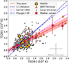 |
Fig. 7. Relation between T[O III] and T[O II] for the MARTA sample (gold hexagons), compared with various samples from the literature at low (grey dots) and high redshifts (from JWST archival data, orange triangles). The plot also shows the 1:1 relation (dashed blue line) and two empirical calibrations of the T2 − T3 relation, from Pilyugin et al. (2009, dashed purple line) and Garnett (1992, dashed magenta line). The red squares represent the median values of the entire sample, binned in T3, with uncertainties given by the standard deviation within each bin. The red line shows the best-fit relation derived in this work. |
For high-z studies, we compiled the emission line fluxes where available and re-derived the electron temperatures employing the same methodology as for MARTA galaxies, which includes adopting a self-consistent set of atomic parameters. In fact, using different sets of collision strengths results in temperature estimates that can differ by ≳500 K, especially for the O++ ion (Nicholls et al. 2013). Therefore, when only temperatures were tabulated but we had no access to the measured line fluxes, we corrected the compiled temperatures to account for such a discrepancy, if needed.
In particular, we used PYNEB to model the difference in the inferred T3 from the Palay et al. (2012) dataset (employed in this work) and the datasets from Storey et al. (2014) and Aggarwal & Keenan (1999) (which provide comparable results to each other), and applied such an offset to the T3 values from the literature that were derived adopting either of the two latter atomic parameters (as in e.g. Chakraborty et al. 2025). This approach brings all T3 values analysed in this work to a consistent scale. Such a correction was not required for T2 as all the literature studies considered adopted the same atomic parameters.
We also compared these data with a large compilation of measurements in low-redshift galaxies (small grey points in Fig. 7), for which we compiled emission-line fluxes and re-measured temperatures self-consistently with the high-z sample. In particular, we included data from low-metallicity local emission-line galaxies from Izotov et al. (2009) and Guseva et al. (2009, 2011); the Curti et al. (2017) sample, consisting of composite spectra of SDSS Data Release 7 star-forming galaxies stacked based on their combined [O II]/Hβ and [O III]/Hβ flux ratios; a sample of SDSS galaxies where both oxygen auroral lines were detected in individual objects (see e.g. Pilyugin et al. 2012); the CHAOS data targeting H II region in massive local spiral galaxies with the MODS spectrograph on the LBT (Large Binocular Telescope) (Berg et al. 2015, 2020; Rogers et al. 2021, 2022); the stacks of Khoram & Belfiore (2025), which consist of spatially resolved spectra from SDSS-IV MaNGA (Mapping Nearby Galaxies at Apache Point Observatory) stacked in bins across the M⋆–SFR plane; and the Zurita et al. (2021) compilation of 2831 published H II region emission-line fluxes in 51 nearby spiral galaxies. In all these cases we recovered the measured extinction-corrected fluxes and re-calculated temperatures following the same approach used for the MARTA data, applying a uniform S/N > 3 cut on the auroral lines.
Furthermore, in Fig. 7 we also plotted some empirical calibrations of the T2 − T3 relation. In particular, Pilyugin et al. (2009) calibrated the relation on a sample of H II regions from the local Universe, while Garnett (1992) provided a fit based on photoionisation models.
Some galaxies in the local sample exhibited evident contamination from [Fe II] (e.g. Curti et al. 2017; Rogers et al. 2021; Hamel-Bravo et al. 2024, see also Moreschini et al., in prep.). This contamination led to artificially elevated T3 values due to the consequent overestimation of the [O III]λ4363 flux. To exclude contaminated galaxies in our analysis, we applied an empirical cut (discussed in Moreschini et al., in prep) defined as log(R/R3) > − 2.1 + log(O32), where R ≡ [O III] λ4363/Hβ, as contaminated. This cut ensured the exclusion of the vast majority of the SDSS stacks flagged as contaminated by Curti et al. (2017) through visual inspection.
The MARTA data shown in Fig. 7 (orange hexagons) exhibit significant scatter, which is also evident in the data from local galaxies in the literature (grey points, typical errors shown in light grey). The red squares in Fig. 7 indicate the median values for the whole sample, binned in T3, with error bars reporting the standard deviation within each bin. The binning was chosen to ensure a minimum of five galaxies per bin, adapting the bin width in the high-T3 regime, where the data are more sparsely sampled. The red line represents a linear fit derived in this work, based on the entire sample. This fit was performed using an orthogonal linear regression algorithm, applied to the median values rather than individual points, to reduce the influence of sampling effects in the diagram. The best-fit linear relation is given by
 (1)
(1)
The slope obtained from our fit is significantly shallower than those reported by, for example, Garnett (1992) and Pilyugin et al. (2009). This effect arises from the inclusion of high-temperature points, which tend to be systematically lower in T2 than in T3 when T3 > 14 000 K. This behaviour is seen consistently in both low- and high-redshift data. This high-T3 range is, however, populated by only ∼30 data points in our large compilation and has therefore been previously hard to confirm observationally in the literature. Hints of this behaviour were, however, already observed by Méndez-Delgado et al. (2023a) and Arellano-Córdova & Rodríguez (2020) when studying the T[N II]–T[O III] relation.
We performed an alternative fit considering only the range T3 = [7000 − 14 000] K, and we obtained a steeper slope of 0.64 ± 0.04, closer to previous calibrations. Furthermore, we compared our orthogonal fit with the median values of the bin with a Bayesian fit performed on individual points using the LINMIX method (Kelly 2007). The results are consistent within two sigma, with the Bayesian fit yielding a slope of 0.50 ± 0.03 and an intercept of 5510 ± 330 K.
We find that the T2 − T3 relation is affected by significant scatter across redshift. This scatter could reflect both observational uncertainties and the adoption of different atomic datasets, as well as be driven by the combination of different physical processes (see Sect. 6.3). For instance, the use of [O II] as a tracer of the low-ionisation zone temperature is particularly controversial. While models predict that T[O II] should be comparable to T[S II] and T[N II] (Campbell et al. 1986; Pilyugin et al. 2006), in practice T[O II] tends to overestimate the temperature compared to T[N II] and T[S II] (Zurita & Bresolin 2012; Curti et al. 2017; Berg et al. 2020; Méndez-Delgado et al. 2023b). This discrepancy may be explained by density inhomogeneities within H II regions, which affect the [O II] and [S II] ratios but have little impact on the [N II] lines (Méndez-Delgado et al. 2023b), as well as from the effect of recombination on the emissivity of the [O II] auroral doublet.
Nonetheless, our observations shows that high-z systems are overall consistent with the distribution of local galaxies on the T2 − T3 relationship, with no systematic offset observed. This finding is in good agreement with the independent analysis by Sanders et al. (2025), who likewise report no evidence of an evolution of the T2 − T3 relation with redshift. This consistency suggests that, while the relationship is not particularly tight, the underlying physical processes governing T2 and T3 do not vary significantly across cosmic time.
6.3. Dependence of the T2–T3 relation on additional physical parameters
We explored the possible dependence of the T2 − T3 relation on additional physical properties to probe the origin of the observed scatter. In particular, we considered three physical parameters: electron density derived from the [S II] ratio (ne), the [O III]/[O II] line ratio as a proxy for the ionisation parameter, and the softness parameter (Vilchez & Pagel 1988), defined as
![Mathematical equation: $$ \begin{aligned} \eta \equiv \frac{([\mathrm{O}\,ii ]3726 + [\mathrm{O}\,ii ]3729)/([\mathrm{O}\,iii ]4959 + [\mathrm{O}\,iii ]5007)}{([\mathrm{S}\,ii ]6730 + [\mathrm{S}\,ii ]6716)/([\mathrm{S}\,iii ]9069 + [\mathrm{S}\,iii ]9532)}\cdot \end{aligned} $$](/articles/aa/full_html/2025/11/aa54843-25/aa54843-25-eq3.gif) (2)
(2)
This parameter is used as a proxy for the hardness of ionising radiation, with a secondary dependence on gas-phase metallicity and other nebular parameters. Since galaxies at high redshifts are known to show a different distribution in these three parameters compared to their low-redshift counterparts (e.g. Sanders et al. 2016; Kaasinen et al. 2018), a dependence of the scatter or the residuals of the T2 − T3 relation on these parameters would provide evidence of a potential redshift evolution.
Figure 8 presents six panels displaying the T2 − T3 relation colour-coded by [O III]/[O II], ne, and η for both individual points and hexagonal bins. The hexagonal bins were computed with a minimum of five objects per bin to ensure statistical robustness. The η diagram contains fewer data points compared to the first two, as only some galaxies in our sample had detections of all four emission lines required to compute η. In particular, the [S III] λ9070,9532 are not available for SDSS galaxies, as they fall outside the observed spectral coverage.
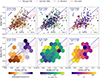 |
Fig. 8. Dependence of the T2 − T3 relationship on different physical properties. Top row: Individual data points. Bottom row: Corresponding hexagonal binning. The colour-coding indicates the three selected physical properties, computed as median values within each bin in the bottom panels: the [O III]/[O II] line ratio (left), the electron density ne (centre), and the softness parameter η (right). In the top panels, MARTA objects are shown as hexagons and low-redshift galaxies as circles. The plots also include the Pilyugin et al. (2009) relation, the Garnett (1992) relation, the 1:1 relation, and our best-fit model. The direction of maximum variation in the colour-coded quantity, determined by the gradient angle, is indicated by navy arrows, with the associated uncertainty shown for reference as light blue arrows. This provides a visual representation of how each parameter varies across the T2 − T3 plane. |
To assess potential correlations between the temperatures, gas density, [O III]/[O II] ratio, and η, we conducted a partial correlation analysis on the full sample, including both local and high-redshift galaxies, using both individual data points and hexagonal bins. The corresponding partial correlation coefficients (r), 95% confidence intervals (CI95%), and p-values are summarised in Table 3. The table reports all partial correlation coefficients computed for both binned and non-binned data, enabling a direct comparison of the two approaches.
Results of the partial correlation analysis on the T2 − T3 relation.
The results indicate that both T3 and T2 exhibit a strong positive correlation with the [O III]/[O II] ratio. This correlation is significantly stronger when computed on the hexagonal bins compared to individual data points, suggesting that binning reduces scatter and enhances the underlying trend. However, the correlation is statistically significant in both cases, confirming its robustness.
In contrast, T2 and T3 exhibit weak correlations with gas density, both from single points and binned data. However, a marginally significant (∼2 − 4σ) positive correlation is observed between T2 and density. The stronger correlation between T2 and density (compared to T3 and density) may arise because the [S II] and [O II] diagnostics, being low-ionisation tracers, probe similar gas regions more effectively than [O III] and [S II]. Moreover, the [O II] auroral-to-nebular line ratio used for temperature diagnostics is highly sensitive to density variations, potentially inducing a spurious trend. A more comprehensive assessment of this trend would require density diagnostics for higher-ionisation lines, which could provide a more detailed representation of the emitting gas distribution and allow us to test a potential dependence of T3 on density.
Regarding η, the results exhibit a strong dependence on binning, with substantial differences between binned and non-binned analyses. In the non-binned data, strong and seemingly significant negative correlations are observed with both temperatures. However, the correlation with T2 is likely driven by a sparsely populated region at high T3 and high η, which skews the overall trend downwards. These high-T3, high-η data points are absent in the binned analysis, leading to a much weaker correlation in the hexbin results. In contrast, the correlation with T3 remains more robust, as it persists in both the binned and non-binned cases, suggesting a more intrinsic relationship between T3 and η.
To further explore these trends, we examined the gradient angle of the colour-coded parameters within the T2 − T3 plane, which is displayed as a navy arrow in each panel of Fig. 8. The gradient angle represents the direction of maximum variation in a given physical parameter (e.g. [O III]/[O II]) and is computed as
 (3)
(3)
where rT2, Z and rT3, Z are the partial correlation coefficients of T2 and T3 with a given property Z (see e.g. Bluck et al. 2019; Curti et al. 2022; Baker et al. 2023). We quantified the uncertainty in the gradient angle via a bootstrapping procedure, randomly resampling the dataset (with replacement) 300 times and recalculating the angle for each iteration. The standard deviation of the resulting angle distribution provides the error, represented by the light blue arrows in Fig. 8. We tested using a larger number of samples for bootstrapping and the inferred uncertainty remains consistent.
Notably, the large errors observed in the central panels of Fig. 8 reflect the weak statistical significance of the partial correlation analysis for ne. The visual near-alignment of the [O III]/[O II] gradient angle with the best-fit T2 − T3 relation seems to point that the orthogonal scatter within this relation is not strongly correlated with this parameter. Such a correlation could arise from a metallicity-driven effect. In fact, a higher metallicity leads to softer ionising spectra (McGaugh 1991; Bresolin et al. 1998), lowering the ionisation parameter and reducing the [O III]/[O II] ratio. Conversely, a lower metallicity results in higher ionisation parameters and [O III]/[O II] ratios (Grasha et al. 2022; Ji & Yan 2022). Since lower-metallicity environments also exhibit higher temperatures, this trend naturally explains the observed correlation. Nevertheless, a more quantitative assessment is needed to robustly evaluate the contribution of the ionisation parameter to the scatter around the T2 − T3 relation.
In addition, we performed an alternative correlation analysis based on the residuals of the T2 − T3 relation relative to our best-fit linear fit in Eq. (1). In particular, we defined the quantity ΔT for each point in the sample as its orthogonal deviation from Eq. (1), measured as (ΔT)2 = (ΔT3)2 + (ΔT2)2. We then calculated the Spearman correlation coefficient between ΔT and each of the physical parameters involved in the analysis. The results reveal a mild yet statistically significant positive correlation (coefficient of 0.15, significant at ∼3σ) between the amplitude of the offset from the temperature relation ΔT and the [O III]/[O II] ratio. This suggests that, although the effect is not dominant, variations in the ionisation parameter – as traced by [O III]/[O II] – do contribute to the scatter around the T2 − T3 relation.
In contrast, both ne and η show minimal effect and weak statistical significance. These results suggest that the orthogonal scatter relative to the best-fit relation does not exhibit a clear dependence-at least not one detectable from the residuals-on these two quantities.
6.4. Sulphur temperatures
Sulphur is a valuable tracer of ionised gas conditions in galaxies, as its ionisation states probe different regions of the ISM. The ionisation potentials of [S III] and [S II] ions are slightly different from those of [O III] and [O II]; the former trace intermediate- and the latter low-ionisation regions. Comparing sulphur and oxygen temperatures is therefore a useful diagnostic for understanding the ionisation structure of H II regions and testing photoionisation models.
The availability of reliable detections of sulphur auroral lines in some of our selected high-redshift galaxies presents a valuable opportunity to compare such temperatures. Our work marks one of the first instances where this relationship is examined for galaxies at high redshifts (Rogers et al. 2024; Welch et al. 2024, 2025; Morishita et al. 2025). Photoionisation models predict that T[S II] ≈ T[O II] (Campbell et al. 1986; Pilyugin et al. 2006; Méndez-Delgado et al. 2023). T[O III], on the other hand, is expected to be higher than T[S III] for [O II] temperatures higher than 8000 K (Garnett 1992). Substantial deviations from both these trends have, however, been observed in extragalactic H II regions (Kennicutt et al. 2003; Esteban et al. 2009; Berg et al. 2015; Croxall et al. 2016; Rogers et al. 2021).
As shown in Fig. 9, the observed trends between the temperatures of sulphur and oxygen ions are consistent with the previous literature and empirical calibrations. In particular, we compared the MARTA objects with extragalactic H II regions (Esteban et al. 2009, 2014, 2020; Domínguez-Guzmán et al. 2022; Rogers et al. 2022). The left panel of Fig. 9 shows the T[S II]–T[O II] relation and the empirical calibration by Méndez-Delgado et al. (2023a), based on local H II regions. Our high-redshift sample lies systematically below the 1:1 relation, but such a trend aligns with the findings of Méndez-Delgado et al. (2023a), who also report an offset in the relation, with [O II] temperatures generally higher than [S II] ones. They attributed this effect to the presence of density fluctuations.
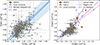 |
Fig. 9. Left panel: T[S II]–T[O II] relation for MARTA objects, compared with extragalactic H II regions together with the empirical calibration by Méndez-Delgado et al. (2023b), based on local H II regions. Right panel: T[S III]–T[O III] relation for MARTA objects, along with local H II region data and two high-redshift galaxies with archival JWST data (Rogers et al. 2024; Welch et al. 2025). The plot also shows the calibrations from Garnett (1992) and Rogers et al. (2021). |
In the right panel of Fig. 9 we show the T[S III]–T[O III] relation. This plot also includes the sample of H II regions from CHAOS (Berg et al. 2015, 2020; Croxall et al. 2015, 2016), and three high-redshift galaxies: the Sunburst Arc (Welch et al. 2025), Q2343-D40 from Rogers et al. (2024), and ID60001 from Zhang et al. (2025), which, to the best of our knowledge, are the only other galaxies at high redshifts with simultaneous measurements of the [S III] and [O III] auroral lines. The figure also shows two calibrations from the literature. The relation in Garnett (1992) was based on photoionisation models and the one in Rogers et al. (2021) was calibrated on local H II regions from the CHAOS survey.
The relation appears somewhat scattered but is still broadly consistent with results from the local literature and comparable to the other high-redshift galaxies. This result is also consistent with the recent findings of Sanders et al. (2025), who reported no evidence of systematic redshift evolution in T − T relations involving sulphur ions. In models, these two temperatures are not always equal, since [S III] and [O III] likely trace different ionisation zones due to their significantly different ionisation potentials, as discussed in Berg et al. (2021).
Quantitatively, our T[S II] measurements show an average negative offset of ∼930 K from the one-to-one relation and ∼470 K from the Méndez-Delgado et al. (2023a) relation. These correspond to average deviations of 1.14σ and 0.52σ (considering our estimates of the temperatures error bars), respectively, indicating that our measurements remain well within expectations based on previous studies. Notably, three out of the four galaxies lie directly on the best-fit relation of Méndez-Delgado et al. (2023b), while the fourth remains consistent within the best-fit uncertainty range.
Similarly, for T[S III], we find the average of the absolute value offset to be 1.9σ from the 1:1 relation, while the offsets relative to Garnett (1992) and Rogers et al. (2021) are 1.9σ, and 2σ, respectively. This time the offset is not systematically negative but the data scatter around the relation.
7. Strong-line metallicity diagnostics and calibrations
Strong-line methods based on combination of nebular lines ratios including [O II]λλ3726,3729, [O III]λ4959, λ5007, and [N II]λ6584 are a valuable way to measure the metallicity of galaxies, in virtue to their brightness and ease of detection across a wide range of redshifts (Maiolino & Mannucci 2019). Nonetheless, the redshift evolution in the physical conditions that are at the basis of the (either direct or indirect) dependence between the involved line ratios and metallicity possibly translates into biases when using such methods to derive the metallicity from high-z spectra adopting diagnostics calibrated on local galaxy samples (Bian et al. 2018; Sanders et al. 2021).
The advent of JWST promised to directly tackle this issue by delivering robust auroral lines detections in high-z galaxies, and this was indeed one of the key objectives of several programmes within the first few cycles. In this section we combine Te-based metallicity measurements for MARTA galaxies with a compilation of measurements from the literature at different redshifts, and test the validity and evolution of various classical strong-line calibrations in the high-z Universe.
7.1. Oxygen abundance determination
We derived the ionic abundances of the O+ and O++ ions in the MARTA golden sample galaxies leveraging the direct measurement of the respective temperatures and employing the GetIonicAbundances routine in pyNeb. To measure the O+ abundance in the MARTA silver sample, we inferred the T2 from the T3 as measured from [O III]λ4363/[O III]λ5007 ratio adopting our newly derived fit of Eq. (1). The total oxygen abundance is then computed as the sum of these two ionic abundances, with the contribution from higher ionisation states like O3+ assumed to be negligible. The results of these abundance calculations are presented in Table 2.
Polynomial coefficients of the best fit for the strong-line metallicity diagnostics.
In addition, we complemented our sample with literature NIRSpec data of galaxies that were detected in the [O III] λ4363 line. We compiled the fluxes (where publicly available) and self-consistently performed extinction correction, temperature, and abundance calculations following the same methodology applied for the MARTA silver sample. The literature sample includes data from D’Eugenio et al. (2024), Navarro-Carrera et al. (2024), Sanders et al. (2024), Schaerer et al. (2024), Arellano-Córdova et al. (2025), Curti et al. (2025b), Morishita et al. (2025), Napolitano et al. (2025), Scholte et al. (2025), Stiavelli et al. (2025), Topping et al. (2025b). Our total sample, combining MARTA and literature sources, consists of 128 galaxies.
As not all strong lines are always detected in literature objects (because of either low sensitivity or limited spectral coverage), each strong-line ratio can be effectively measured in a different number of objects, as reported in each panel in Fig. 10. As an example, for R23 we present a calibration based on 96 objects, nonetheless nearly doubling previous largest compilation of Chakraborty et al. (2025).
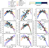 |
Fig. 10. Nine different strong-line diagnostics comparing our MARTA data (striped hexagons for the golden sample, plain hexagons for the silver) with high-z literature samples (crosses) and a set of empirical calibrations. The data are colour-coded by redshift bin. The high-redshift data include strong-line calibration measurements from JWST surveys (D’Eugenio et al. 2024; Navarro-Carrera et al. 2024; Sanders et al. 2024; Schaerer et al. 2024; Arellano-Córdova et al. 2025; Curti et al. 2025b; Morishita et al. 2025; Napolitano et al. 2025; Scholte et al. 2025; Stiavelli et al. 2025; Topping et al. 2025b). The empirical calibration curves from the local Universe are from Maiolino et al. (2008), Bian et al. (2018), Curti et al. (2020a), and Nakajima et al. (2022), colour-coded in a dark colour palette (blue, purple, green), while the high-redshift-based calibrations from Sanders et al. (2024) and Chakraborty et al. (2025) are represented with a warm colour palette (yellow, orange, and red). Dashed lines denote extrapolations of the calibrations outside the regime where they have been calibrated. Our best-fit relations to the high-redshift dataset are shown in red. In most cases, a third-degree polynomial was used; for the N2 and R2 diagnostics, we adopted a linear fit, as there were no particular features that required a higher-order polynomial. Furthermore, in the |

7.2. New JWST-based metallicity calibrations
In Fig. 10 we show the position of our combined JWST sample on different strong-line ratios diagnostics versus metallicity diagrams. MARTA galaxies primarily occupy the high-metallicity end of the distribution, a region largely unexplored at high redshifts. We compare our combined sample with empirical calibration derived from both local and high-redshift galaxy studies.
The local calibrations we considered include those from Maiolino et al. (2008), which are based on low-metallicity galaxies from Nagao et al. (2006) and photoionisation model-based oxygen abundances for SDSS galaxies in the high-metallicity regime. We also included the calibrations by Curti et al. (2017), later revisited in Curti et al. (2020b), which are based on stacked spectra of SDSS galaxies; and those by Nakajima et al. (2022), who extended the Curti et al. (2017) SDSS stacks by including extremely metal-poor galaxies from the EMPRESS survey. Additionally, we used the calibrations by Bian et al. (2018), derived from stacked spectra of local high-redshift analogues selected based on their location on the [N II]-BPT diagram.
For comparison, we also included recent works that recalibrate the same strong-line diagnostics using JWST data. In particular, we considered the calibrations from Sanders et al. (2024), based on galaxies at z = 2 − 9 from the CEERS survey Finkelstein et al. (2023), and those from Chakraborty et al. (2025), based on galaxies from the CEERS, JADES (D’Eugenio et al. 2025), and UNCOVER (Bezanson et al. 2024) surveys, with fluxes compiled by the PRIMAL project (Heintz et al. 2025).
All curves corresponding to the different calibrations shown in Fig. 10 are plotted as solid lines within the directly probed metallicity range, while polynomial extrapolations beyond the calibration range are shown as dashed lines. We also provide new fits to the strong-line ratios as a function of metallicity based on the full JWST sample compiled in this work. The fitting procedure was implemented as a direct polynomial regression, where the coefficients were optimised using the least_squares routine from the SCIPY library. To limit the influence of individual outliers, we adopted the Huber loss function4. This approach retains the efficiency of least-squares fitting in the well-sampled regime, while improving robustness in the presence of non-Gaussian scatter. In most cases, we adopted a third- or a forth-order polynomial, while for the N2 diagnostic, which does not exhibit significant curvature, we opted for a linear model.
These polynomial fits are constrained by observations in the range 12 + log(O/H) ∈ [7.0−8.4]. Outside this interval, the lack of direct constraints makes extrapolation highly uncertain. To stabilise the behaviour at low and high metallicities, the fits were regularised by anchoring them to the analytic calibrations of Curti et al. (2017). In practice, we introduced additional constraint points at metallicities beyond the observed range, with target values set by these empirical relations. These points were assigned enhanced weights in the loss function, ensuring that the fits remain driven by the data where observations are available, while gradually converging to the expected trends at the boundaries. The regression was performed on metallicities normalised to the solar abundance (12 + log(O/H) = 8.69), so that the best-fit coefficients reported in Table 4 are expressed as functions of the normalised abundance Znorm = (12 + log(O/H)) − 8.69. The resulting calibrations are shown in red in Fig. 10. We did not report fits for the O3N2 diagnostic, for reasons discussed below. The calibrations presented in this work are based on a dataset that is potentially biased since we only based the calibrations on a subset of galaxies for which auroral lines have been detected, favouring systems with elevated SFRs. Such biases are intrinsic to all calibrations based on auroral lines, including those derived from local objects. We address this issue in more detail in Appendix E.
7.2.1. The R23, R3, and R2 diagnostics
Among the newly calibrated relationships, R23 is characterised by the lowest scatter, in agreement with previous analyses (Nakajima et al. 2022; Sanders et al. 2024; Chakraborty et al. 2025). However, the R23 calibration exhibits a well-known double-branched structure, with most galaxies populating the plateau region where the relationship flattens, severely limiting its accuracy at intermediate metallicities. A similar behaviour is also observed in R3, where the turnover occurs around 12 + log(O/H) ∼ 8.0, leading to two distinct metallicity solutions.
R2 is generally not employed alone for metallicity measurements due to its sensitivity to the ionisation parameter. However, it can assist in resolving ambiguities in the R23 and R3 calibrations. In our sample, R2 shows an increasing trend with metallicity, although with a much larger scatter in the line ratios at fixed O/H than observed for R3 and R23.
7.2.2. O32, Ne3O2, O3N2, and O3S2 diagnostics
Alternative diagnostics such as O32, Ne3O2, O3N2, and O3S2 also display large scatter, highlighting the challenges in metallicity estimation when these indicators are used individually. While O32 primarily traces the ionisation parameter, which is correlated with metallicity (Ji & Yan 2022), other ratios are also sensitive to possible variations in the neon, nitrogen, and sulphur abundance patterns. The scatter is particularly pronounced in the low-metallicity regime. Nonetheless, O32 and Ne3O2 show a monotonic trend with metallicity (with Ne3O2 being also almost insensitivity to reddening) and, hence, remain a valuable tool for differentiating between metallicity solutions, especially when used alongside diagnostics such as R23 (e.g. Kewley & Dopita 2002). O3S2 was excluded from the fitting procedure due to the limited number of available data points and the high level of scatter observed.
Interestingly, we identify a subset of z ∼ 2 low-metallicity galaxies in the MARTA sample that showcase intense emission in the low-ionisation species, which makes them deviate significantly from the average relation, displaying enhanced [O II]/Hβ (and [S II]/Hβ) ratios given their O/H. These galaxies also exhibit elevated [N II]/Hα ratios (as also mentioned in Sect. 7.2.3), and correspondingly low [O III]/[N II] and [O III]/[S II] values, suggesting a systematic offset in multiple diagnostic line ratios. While dust attenuation uncertainties – such as deviations from the assumed attenuation law – could affect line ratios involving widely separated wavelengths (e.g. [O II]/Hβ), they are unlikely to fully explain the broad pattern of anomalies observed across both nearby and closely spaced lines. Conversely, MARTA galaxies at z > 3 are characterised by some of the lowest [O II]/Hβ values measured in the JWST sample. Such a spread, observed also in extremely metal-poor galaxies in the local Universe (Nakajima et al. 2022), highlights the role of intense star formation and varying ionisation conditions in shaping the relationship between strong-line ratios andmetallicity.
At low metallicities, galaxies typically exhibit higher ionisation parameters; however, the ionisation conditions are not uniform across different systems (e.g. Grasha et al. 2022), but they are strongly modulated by variations in the SFR (e.g. Ji & Yan 2022), the geometric distribution of the gas, and the presence of young, hot stellar populations. Consequently, low-ionisation tracers such as [N II] and [S II] display significant scatter, reflecting the intrinsic diversity in ionisation conditions within low-metallicity environments. Given that our sample is relatively small, the presence of multiple such cases suggests that these conditions are more common at high redshifts than previously thought.
Median offset and dispersion (scatter) in line ratios at fixed O/H for each diagnostic and calibration considered in this work.
7.2.3. The N2 diagnostic
Thanks to JWST we can start populating the low-metallicity region of the N2 diagnostic. In line with well-established findings over the past decade from ground-based spectroscopic surveys such as MOSDEF (Shapley et al. 2015), KBSS (Steidel et al. 2014; Strom et al. 2018), KLEVER (Hayden-Pawson et al. 2022), and FMOS (Fiber Multi-Object Spectrograph) (Kashino et al. 2017), high-z galaxies exhibit an offset in the [N II]-BPT diagram (Fig. 3), with enhanced [N II]/Hα compared to their local counterparts. One of the most widely accepted interpretations of this behaviour is the hardening of the ionising radiation field at high redshifts, which-at fixed metallicity-shifts the [N II]/Hα ratio to higher values without necessarily implying variations in chemical abundance patterns (Topping et al. 2020).
We observe the same deviation in the [N II]/Hα versus O/H relation compared to local calibrations, at least at low metallicities (12 + log(O/H) < 8). The possible role of enhanced N/O ratios in driving this offset has been recently investigated using the EXCELS dataset (Scholte et al. 2025), where a correlation between N/O and the degree of offset from the median calibration was reported, both at high and low redshifts. An analysis of the N/O abundance in our combined sample will be the subject of a future study.
At z > 6 the optical [N II] is rarely detected because it falls outside the wavelength range probed by JWST/NIRSpec, but also because galaxies at these redshifts tend to have low metallicities and high ionisation parameters, possibly causing most of the nitrogen to reside in higher ionisation states. Thus, the absence of [N II] in high-z sources may also result from nitrogen being predominantly in higher ionisation states (probed by N III], N IV]), as suggested by recent JWST findings (Bunker et al. 2023; Cameron et al. 2023b; Charbonnel et al. 2023; Isobe et al. 2023; Ji et al. 2024; Marques-Chaves et al. 2024; Schaerer et al. 2024; Topping et al. 2024; Curti et al. 2025b).
7.2.4. The  diagnostic
Finally, we tested the  diagnostic proposed by Laseter et al. (2024) and recently re-calibrated by Scholte et al. (2025) based on a combined sample of data from the JWST/EXCELS survey (Carnall et al. 2024) and new local galaxy measurements from the DESI Early Data Release (DESI Collaboration 2022). Although at high metallicities (Z ≈ Z⊙) the high-z dataset lacks sufficient coverage to constrain the turnover of the functional form, performing a fit with the same functional form as in Laseter et al. (2024) to the combined JWST sample provides very similar behaviour to the original calibration in the low-metallicity branch (which is the one primarily populated by high-z galaxies).
While very similar in shape, the Scholte et al. (2025) calibration appears slightly offset towards higher  ratios at low metallicities compared to both the original Laseter et al. (2024) parametrisation and to our current fit. This discrepancy may be caused by intrinsic differences in the calibration samples, but differences in the set of adopted atomic parameters for O++ could also play a role. Variations of up to ∼500 K in the T3 derivation (see the discussion in Sect. 6) translate into a difference in the final inferred O/H of ∼0.02 − 0.04 dex at fixed line ratios and at low metallicities (12 + log(O/H) ∼ 7.5), where the total abundance budget is dominated by doubly ionised oxygen. Ultimately, we cannot provide the coefficients for the new fit to the
  diagnostic, as our data do not offer significant additional constraints compared to Laseter et al. (2024).
7.3. Comparison with literature calibrations
We analysed the behaviour of each calibration curve considered in this work by computing, for the combined JWST high-z galaxy sample, the offset between observed and predicted line ratios at fixed 12 + log(O/H). We report the median offset and the associated dispersion for each diagnostic and calibration in Table 5. Beside the new calibrations provided in this work (for which the scatter in the calibration sample is minimised by definition), the calibrations presented in Sanders et al. (2024) and Chakraborty et al. (2025) behave well. The two were based on similar (though smaller) samples of high-z galaxies. In contrast, most of the calibrations based on local galaxy samples show larger offsets, as expected given the evolving physical conditions of the calibration samples.
To better visualise possible trends with metallicity, in Fig. 11 we plot the median offset in the line ratio computed in 0.15 dex bins of metallicity, as a function of 12 + log(O/H) (where only bins containing at least five objects are considered). Figure 11 highlights the discrepancy between the local (z ∼ 0) calibrations and the high-redshift galaxy sample. In diagnostics like R3, R23, and O32, the local calibration curves (e.g. Maiolino et al. 2008; Curti et al. 2020b; Nakajima et al. 2022) tend to lie below the observed data points for high-redshift galaxies, suggesting a redshift-dependent evolution of these ratios. Such evolution must be factored into metallicity measurements for high-redshift galaxies. Sanders et al. (2025) also recently reported a clear redshift evolution in oxygen-based strong-line calibrations, with high-redshift galaxies showing offsets consistent with hotter stellar populations and harder ionising spectra relative to local samples. This reinforces the need to account for cosmic evolution when applying local calibrations to earlygalaxies.
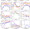 |
Fig. 11. Median offset of the strong-line calibrations analysed in this work relative to the high-z sample (z ∼ 1 − 9.5), computed in bins of metallicity. The bins have a width of 0.15 dex and are included only if they contain at least five objects. Each panel corresponds to a different diagnostic. The colour palette is the same as used in Fig. 10 to distinguish between low-z and high-z based calibrations, with markers also representing this division: stars for high-z and squares for z ∼ 0 based calibrations. |
However, we observe that for several calibrators the median offset tends to decrease with increasing metallicity, possibly suggesting a metallicity-dependent redshift evolution of the involved strong-line diagnostics. This is in line with the observed increase in the scatter of line ratios at fixed O/H in the low-metallicity regime.
As the typical ionisation conditions of the ISM in galaxies evolve with cosmic time, we would expect this behaviour to be reflected into a trend between the dispersion of each calibration and redshift. Although the combined JWST sample analysed in this work is still too small to perform a robust analysis of the ‘internal’ redshift evolution (between z ∼ 1 and z ∼ 10), hints of such a correlation are already visible for some of the diagnostics in Fig. 10, and are better visualised in Fig. 12, where we display the offsets in line ratios for individual high-z sources from the best-fit relationships recalibrated in this work, colour-coded by galaxy redshift. At low metallicities (12 + log(O/H) ≲ 8), galaxies at the lower-redshift boundary of the JWST sample tend to be offset in the opposite direction to the highest-redshift systems from the best-fit calibration, especially in line-ratio diagnostics where the dependence on the ionisation parameter is more prominent such as R2, O32, and Ne3O2.
8. Summary and outlook
In this work we have analysed deep JWST/NIRSpec R1000 spectra of 16 star-forming galaxies at 1.8 < z < 4.7, observed in the framework of the MARTA programme. We report the detection of faint auroral lines, including [O III] λ4363, [O II] λλ7320,7330, [S II] λλ4068,4076, and [S III] λ6312 (Figs. 4 and 6), derived Te-based metallicities, and discuss trends in the temperature-temperature relationships and the evolution of strong-line metallicity calibrations. The key results from this work are summarised as follows.
-
The temperature-temperature (T2 − T3) relation between different oxygen ionised species, established on low-redshift samples, seems to hold at earlier cosmic epochs, offering, despite its non-negligible scatter, a reliable framework for metallicity determinations at high z (Fig. 7).
-
The dispersion of the T2 − T3 relationship mainly correlates with variations in the ionisation parameter (traced by [O III]/[O II]) and/or in the hardening of the ionising continuum (traced by the ‘softness parameter’, η; Fig. 8 and Table 3). Variations in the electron density mainly correlate with T2 (at fixed T3) but have a lower impact on the scatter of the relationship.
-
We explored the relationship between temperatures derived for low-ionisation and high-ionisation sulphur and oxygen species, demonstrating their consistency with local trends (Fig. 9).
-
The MARTA auroral-line galaxies, while still subsolar on average, populate the upper end of the metallicity distribution along with high-redshift galaxies with direct metallicity measurements. As such, they provide valuable insights into the applicability of strong-line metallicity calibrations at z ∼ 2, extending beyond the low-metallicity regime typically probed by earlier studies. By combining our sample with existing Te-based metallicity measurements from JWST in the literature, we assessed the redshift evolution in several popular strong-line diagnostics over a wide range of oxygen abundances (12 + log(O/H) ∈ [7.0−8.4]; Figs. 10 and 11) and provide updated calibrations for some of these diagnostics in the form of standard polynomial relations (Table 4).
-
While ‘strong-line methods’ remain broadly applicable across cosmic time, clear systematic shifts emerge in specific line ratios, particularly R2, O32, and Ne3O2, as likely driven by evolving ionisation conditions at high redshifts. This trend is reflected in a correlation between the offset in the line ratio at fixed metallicities and redshifts in these diagnostics, as tentatively observed in our combined JWST sample (Fig. 12).
-
We observe a systematic offset in the N2 versus O/H diagram (especially at low metallicities), in line with previous findings that high-redshift galaxies exhibit higher [N II]/Hα at fixed O/H compared to local counterparts (e.g. Steidel et al. 2014; Masters et al. 2014; Shapley et al. 2015; Strom et al. 2017). Furthermore, a subset of low-metallicity galaxies in the MARTA sample deviates significantly from the average relationships due to their elevated [O II]/Hβ and [S II]/Hβ ratios given their O/H, highlighting the variety of ionisation conditions observed in the high-redshift Universe and the potential impact of selection effects on the determination of the average trends in high-z galaxy populationproperties.
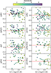 |
Fig. 12. Offsets in the log of the chosen line ratio at fixed O/H, representing the difference between the observed ratio and the value predicted by our best-fit calibrations. High-z JWST sample points are colour-coded by redshift to highlight potential trends. |
Future research will build on the insights gained from this and other recent JWST-enabled studies to achieve a more self-consistent determination of galaxy metallicity properties and their scaling relations across cosmic epochs. In parallel, studies of chemical abundance patterns in high-redshift galaxies, focusing on elements such as nitrogen, neon, and argon, will provide complementary insights into star formation histories at z ∼ 2 and beyond, helping refine next-generation chemical evolution models. A key avenue for future exploration is the derivation of direct, Te-based nitrogen-to-oxygen (N/O) abundance ratios. Variations in N/O ratios at high redshifts can reveal crucial details about rapid nitrogen enrichment, differences in star formation efficiency, or localised enrichment processes such as those driven by Wolf-Rayet stars (Fernández-Martín et al. 2012; Rivera-Thorsen et al. 2024; Kobayashi & Ferrara 2024), highlighting the importance of exploring this diagnosticin detail.
Furthermore, we plan to conduct detailed comparisons with state-of-the-art photoionisation models, such as HOMERUN (Marconi et al. 2024; Moreschini et al., in prep.). Unlike single-cloud models, HOMERUN incorporates contributions from multiple gas clouds with varying metallicities, ionisation parameters, and densities. This approach enables a more nuanced analysis of emission line ratios, allowing us to assess the impact of high-density gas clumps on metallicity determinations and refine our understanding of biases in classicalmethods.
With the exception of one galaxy, MARTA_4327, where such emission is interpreted as stellar in nature and associated with the presence of Wolf-Rayet stars; see Curti et al. (2025a).
The Huber loss behaves as a standard χ2 (L2 norm) for small residuals while reducing the weight of points with large deviations by transitioning to a linear (L1) form.
Acknowledgments
FB and FM acknowledge support from the INAF Fundamental Astrophysics programme 2022 and 2023. FM and FB acknowledge support from grant PRIN-MUR 202223XDPZM “Prometeus” GC and EB acknowledge financial support from INAF under the Large Grant 2022 “The metal circle: a new sharp view of the baryon cycle up to Cosmic Dawn with the latest generation IFU facilities”. A.F. acknowledges the support from project “VLT- MOONS” CRAM 1.05.03.07. AM acknowledges support from project PRIN-MUR project “PROMETEUS” financed by the European Union – Next Generation EU, Mission 4 Component 1 CUP B53D23004750006. FC acknowledges support from a UKRI Frontier Research Guarantee Grant (PI Cullen; grant reference EP/X021025/1). CK acknowledges funding from the UK Science and Technology Facility Council through grant ST/Y001443/1. This work is based in on observations made with the NASA/ESA/CSA James Webb Space Telescope. The data were obtained from the Mikulski Archive for Space Telescopes at the Space Telescope Science Institute, which is operated by the Association of Universities for Research in Astronomy, Inc., under NASA contract NAS 5-03127 for JWST. These observations are associated with program JWST 1879. The data presented in this paper were obtained from the Mikulski Archive for Space Telescopes (MAST). The specific observations analyzed can be accessed via https://doi.org/10.17909/v7wt-1r79. STScI is operated by the Association of Universities for Research in Astronomy, Inc., under NASA contract NAS5–26555.
References
- Aggarwal, K. M., & Keenan, F. P. 1999, ApJS, 123, 311 [NASA ADS] [CrossRef] [Google Scholar]
- Andrews, B. H., & Martini, P. 2013, ApJ, 765, 140 [NASA ADS] [CrossRef] [Google Scholar]
- Arellano-Córdova, K. Z., & Rodríguez, M. 2020, MNRAS, 497, 672 [CrossRef] [Google Scholar]
- Arellano-Córdova, K. Z., Cullen, F., Carnall, A. C., et al. 2025, MNRAS, 540, 2991 [Google Scholar]
- Baker, W. M., Maiolino, R., Belfiore, F., et al. 2023, MNRAS, 519, 1149 [Google Scholar]
- Baldwin, J. A., Phillips, M. M., & Terlevich, R. 1981, PASP, 93, 5 [Google Scholar]
- Balogh, M. L., McGee, S. L., Mok, A., et al. 2014, MNRAS, 443, 2679 [NASA ADS] [CrossRef] [Google Scholar]
- Belfiore, F., Westfall, K. B., Schaefer, A., et al. 2019, AJ, 158, 160 [CrossRef] [Google Scholar]
- Berg, D. A., Skillman, E. D., Croxall, K. V., et al. 2015, ApJ, 806, 16 [NASA ADS] [CrossRef] [Google Scholar]
- Berg, D. A., Pogge, R. W., Skillman, E. D., et al. 2020, ApJ, 893, 96 [NASA ADS] [CrossRef] [Google Scholar]
- Berg, D. A., Chisholm, J., Erb, D. K., et al. 2021, ApJ, 922, 170 [CrossRef] [Google Scholar]
- Bezanson, R., Labbe, I., Whitaker, K. E., et al. 2024, ApJ, 974, 92 [NASA ADS] [CrossRef] [Google Scholar]
- Bian, F., Fan, X., Bechtold, J., et al. 2010, ApJ, 725, 1877 [NASA ADS] [CrossRef] [Google Scholar]
- Bian, F., Kewley, L. J., & Dopita, M. A. 2018, ApJ, 859, 175 [CrossRef] [Google Scholar]
- Bluck, A. F. L., Maiolino, R., Sánchez, S. F., et al. 2019, MNRAS, 485, 666 [Google Scholar]
- Brammer, G. B., van Dokkum, P. G., & Coppi, P. 2008, ApJ, 686, 1503 [Google Scholar]
- Bresolin, F., Kennicutt, R. C., & Garnett, D. R. 1998, ApJ, 510, 104 [Google Scholar]
- Bruzual, G., & Charlot, S. 2003, MNRAS, 344, 1000 [NASA ADS] [CrossRef] [Google Scholar]
- Bunker, A. J., Saxena, A., Cameron, A. J., et al. 2023, A&A, 677, A88 [NASA ADS] [CrossRef] [EDP Sciences] [Google Scholar]
- Calzetti, D., Kinney, A. L., & Storchi-Bergmann, T. 1994, ApJ, 429, 582 [Google Scholar]
- Cameron, A. J., Saxena, A., Bunker, A. J., et al. 2023a, A&A, 677, A115 [NASA ADS] [CrossRef] [EDP Sciences] [Google Scholar]
- Cameron, A. J., Katz, H., Rey, M. P., & Saxena, A. 2023b, MNRAS, 523, 3516 [NASA ADS] [CrossRef] [Google Scholar]
- Campbell, A., Terlevich, R., & Melnick, J. 1986, MNRAS, 223, 811 [NASA ADS] [CrossRef] [Google Scholar]
- Cappellari, M., & Emsellem, E. 2004, PASP, 116, 138 [Google Scholar]
- Cardelli, J. A., Clayton, G. C., & Mathis, J. S. 1989, ApJ, 345, 245 [Google Scholar]
- Carnall, A. C., Cullen, F., McLure, R. J., et al. 2024, MNRAS, 534, 325 [NASA ADS] [CrossRef] [Google Scholar]
- Chabrier, G. 2003, PASP, 115, 763 [Google Scholar]
- Chakraborty, P., Sarkar, A., Smith, R., et al. 2025, ApJ, 985, 24 [Google Scholar]
- Charbonnel, C., Schaerer, D., Prantzos, N., et al. 2023, A&A, 673, L7 [NASA ADS] [CrossRef] [EDP Sciences] [Google Scholar]
- Christensen, L., Laursen, P., Richard, J., et al. 2012, MNRAS, 427, 1973 [NASA ADS] [CrossRef] [Google Scholar]
- Comparat, J., Richard, J., Kneib, J.-P., et al. 2015, A&A, 575, A40 [NASA ADS] [CrossRef] [EDP Sciences] [Google Scholar]
- Conroy, C., Villaume, A., van Dokkum, P. G., & Lind, K. 2018, ApJ, 854, 139 [Google Scholar]
- Cresci, G., Mannucci, F., & Curti, M. 2019, A&A, 627, A42 [NASA ADS] [CrossRef] [EDP Sciences] [Google Scholar]
- Croxall, K. V., Pogge, R. W., Berg, D. A., Skillman, E. D., & Moustakas, J. 2015, ApJ, 808, 42 [NASA ADS] [CrossRef] [Google Scholar]
- Croxall, K. V., Pogge, R. W., Berg, D. A., Skillman, E. D., & Moustakas, J. 2016, ApJ, 830, 4 [NASA ADS] [CrossRef] [Google Scholar]
- Cullen, F., Shapley, A. E., McLure, R. J., et al. 2021, MNRAS, 505, 903 [CrossRef] [Google Scholar]
- Cullen, F., Carnall, A. C., Scholte, D., et al. 2025, MNRAS, 540, 2176 [Google Scholar]
- Curti, M., Cresci, G., Mannucci, F., et al. 2017, MNRAS, 465, 1384 [Google Scholar]
- Curti, M., Maiolino, R., Cirasuolo, M., et al. 2020a, MNRAS, 492, 821 [CrossRef] [Google Scholar]
- Curti, M., Mannucci, F., Cresci, G., & Maiolino, R. 2020b, MNRAS, 491, 944 [Google Scholar]
- Curti, M., Hayden-Pawson, C., Maiolino, R., et al. 2022, MNRAS, 512, 4136 [NASA ADS] [CrossRef] [Google Scholar]
- Curti, M., D’Eugenio, F., Carniani, S., et al. 2023, MNRAS, 518, 425 [Google Scholar]
- Curti, M., Cataldi, E., Belfiore, F., et al. 2025a, ArXiv e-prints [arXiv:2509.06622] [Google Scholar]
- Curti, M., Witstok, J., Jakobsen, P., et al. 2025b, A&A, 697, A89 [Google Scholar]
- Damjanov, I., Zahid, H. J., Geller, M. J., Fabricant, D. G., & Hwang, H. S. 2018, ApJS, 234, 21 [NASA ADS] [CrossRef] [Google Scholar]
- DESI Collaboration (Abareshi, B., et al.) 2022, AJ, 164, 207 [NASA ADS] [CrossRef] [Google Scholar]
- D’Eugenio, F., Maiolino, R., Carniani, S., et al. 2024, A&A, 689, A152 [NASA ADS] [CrossRef] [EDP Sciences] [Google Scholar]
- D’Eugenio, F., Cameron, A. J., Scholtz, J., et al. 2025, ApJS, 277, 4 [Google Scholar]
- Domínguez-Guzmán, G., Rodríguez, M., García-Rojas, J., Esteban, C., & Toribio San Cipriano, L. 2022, MNRAS, 517, 4497 [CrossRef] [Google Scholar]
- Dunlop, J. S., Abraham, R. G., Ashby, M. L. N., et al. 2021, PRIMER: Public Release IMaging for Extragalactic Research, JWST Proposal. Cycle 1, 1837 [Google Scholar]
- Erb, D. K., Steidel, C. C., Shapley, A. E., et al. 2006, ApJ, 647, 128 [NASA ADS] [CrossRef] [Google Scholar]
- Esteban, C., Peimbert, M., García-Rojas, J., et al. 2004, MNRAS, 355, 229 [NASA ADS] [CrossRef] [Google Scholar]
- Esteban, C., Bresolin, F., Peimbert, M., et al. 2009, ApJ, 700, 654 [NASA ADS] [CrossRef] [Google Scholar]
- Esteban, C., García-Rojas, J., Carigi, L., et al. 2014, MNRAS, 443, 624 [NASA ADS] [CrossRef] [Google Scholar]
- Esteban, C., Bresolin, F., García-Rojas, J., & Toribio San Cipriano, L. 2020, MNRAS, 491, 2137 [NASA ADS] [Google Scholar]
- Fernández-Martín, A., Martín-Gordón, D., Vílchez, J. M., et al. 2012, A&A, 541, A119 [NASA ADS] [CrossRef] [EDP Sciences] [Google Scholar]
- Finkelstein, S. L., Bagley, M. B., Ferguson, H. C., et al. 2023, ApJ, 946, L13 [NASA ADS] [CrossRef] [Google Scholar]
- Garnett, D. R. 1992, AJ, 103, 1330 [NASA ADS] [CrossRef] [Google Scholar]
- Garnett, D. R. 2002, ApJ, 581, 1019 [NASA ADS] [CrossRef] [Google Scholar]
- Gordon, K. D., Clayton, G. C., Misselt, K. A., Landolt, A. U., & Wolff, M. J. 2003, ApJ, 594, 279 [NASA ADS] [CrossRef] [Google Scholar]
- Grasha, K., Chen, Q. H., Battisti, A. J., et al. 2022, ApJ, 929, 118 [NASA ADS] [CrossRef] [Google Scholar]
- Guseva, N. G., Papaderos, P., Meyer, H. T., Izotov, Y. I., & Fricke, K. J. 2009, A&A, 505, 63 [NASA ADS] [CrossRef] [EDP Sciences] [Google Scholar]
- Guseva, N. G., Izotov, Y. I., Stasińska, G., et al. 2011, A&A, 529, A149 [NASA ADS] [CrossRef] [EDP Sciences] [Google Scholar]
- Hainline, K. N., Shapley, A. E., Kornei, K. A., et al. 2009, ApJ, 701, 52 [NASA ADS] [CrossRef] [Google Scholar]
- Hamel-Bravo, M. J., Fisher, D. B., Berg, D., et al. 2024, MNRAS, 530, 3855 [Google Scholar]
- Hasinger, G., Capak, P., Salvato, M., et al. 2018, ApJ, 858, 77 [Google Scholar]
- Hayden-Pawson, C., Curti, M., Maiolino, R., et al. 2022, MNRAS, 512, 2867 [NASA ADS] [CrossRef] [Google Scholar]
- Heintz, K. E., Brammer, G. B., Watson, D., et al. 2025, A&A, 693, A60 [Google Scholar]
- Ilbert, O., Arnouts, S., McCracken, H. J., et al. 2006, A&A, 457, 841 [NASA ADS] [CrossRef] [EDP Sciences] [Google Scholar]
- Isobe, Y., Ouchi, M., Tominaga, N., et al. 2023, ApJ, 959, 100 [NASA ADS] [CrossRef] [Google Scholar]
- Izotov, Y. I., Guseva, N. G., Fricke, K. J., & Papaderos, P. 2009, A&A, 503, 61 [NASA ADS] [CrossRef] [EDP Sciences] [Google Scholar]
- Jakobsen, P., Ferruit, P., Alves de Oliveira, C., et al. 2022, A&A, 661, A80 [NASA ADS] [CrossRef] [EDP Sciences] [Google Scholar]
- James, B. L., Pettini, M., Christensen, L., et al. 2014, MNRAS, 440, 1794 [NASA ADS] [CrossRef] [Google Scholar]
- Ji, X., & Yan, R. 2022, A&A, 659, A112 [NASA ADS] [CrossRef] [EDP Sciences] [Google Scholar]
- Ji, X., Übler, H., Maiolino, R., et al. 2024, MNRAS, 535, 881 [NASA ADS] [CrossRef] [Google Scholar]
- Kaasinen, M., Kewley, L., Bian, F., et al. 2018, MNRAS, 477, 5568 [NASA ADS] [CrossRef] [Google Scholar]
- Kartaltepe, J. S., Sanders, D. B., Le Floc’h, E., et al. 2010, ApJ, 709, 572 [Google Scholar]
- Kartaltepe, J. S., Sanders, D. B., Silverman, J. D., et al. 2015, ApJ, 806, L35 [NASA ADS] [CrossRef] [Google Scholar]
- Kashino, D., Silverman, J. D., Sanders, D., et al. 2017, ApJ, 835, 88 [NASA ADS] [CrossRef] [Google Scholar]
- Kauffmann, G., Heckman, T. M., White, S. D. M., et al. 2003, MNRAS, 341, 54 [Google Scholar]
- Kelly, B. C. 2007, ApJ, 665, 1489 [Google Scholar]
- Kennicutt, R. C. 1998, ARA&A, 36, 189 [NASA ADS] [CrossRef] [Google Scholar]
- Kennicutt, R. C., & Evans, N. J. 2012, ARA&A, 50, 531 [NASA ADS] [CrossRef] [Google Scholar]
- Kennicutt, R. C., Bresolin, F., & Garnett, D. R. 2003, ApJ, 591, 801 [NASA ADS] [CrossRef] [Google Scholar]
- Kewley, L. J., & Dopita, M. A. 2002, ApJS, 142, 35 [Google Scholar]
- Kewley, L. J., Dopita, M. A., Sutherland, R. S., Heisler, C. A., & Trevena, J. 2001, ApJ, 556, 121 [Google Scholar]
- Kewley, L. J., Maier, C., Yabe, K., et al. 2013, ApJ, 774, L10 [Google Scholar]
- Kewley, L. J., Nicholls, D. C., & Sutherland, R. S. 2019, ARA&A, 57, 511 [Google Scholar]
- Khoram, A. H., & Belfiore, F. 2025, A&A, 693, A150 [NASA ADS] [CrossRef] [EDP Sciences] [Google Scholar]
- Kisielius, R., Storey, P. J., Ferland, G. J., & Keenan, F. P. 2009, MNRAS, 397, 903 [NASA ADS] [CrossRef] [Google Scholar]
- Kobayashi, C., & Ferrara, A. 2024, ApJ, 962, L6 [NASA ADS] [CrossRef] [Google Scholar]
- Kriek, M., Shapley, A. E., Reddy, N. A., et al. 2015, ApJS, 218, 15 [NASA ADS] [CrossRef] [Google Scholar]
- Laseter, I. H., Maseda, M. V., Curti, M., et al. 2024, A&A, 681, A70 [NASA ADS] [CrossRef] [EDP Sciences] [Google Scholar]
- Le Borgne, D., Rocca-Volmerange, B., Prugniel, P., et al. 2004, A&A, 425, 881 [CrossRef] [EDP Sciences] [Google Scholar]
- Lilly, S. J., Le Brun, V., Maier, C., et al. 2009, ApJS, 184, 218 [Google Scholar]
- Luridiana, V., Morisset, C., & Shaw, R. A. 2015, A&A, 573, A42 [NASA ADS] [CrossRef] [EDP Sciences] [Google Scholar]
- Maiolino, R., & Mannucci, F. 2019, A&ARv, 27, 3 [Google Scholar]
- Maiolino, R., Nagao, T., Grazian, A., et al. 2008, A&A, 488, 463 [NASA ADS] [CrossRef] [EDP Sciences] [Google Scholar]
- Mannucci, F., Cresci, G., Maiolino, R., Marconi, A., & Gnerucci, A. 2010, MNRAS, 408, 2115 [NASA ADS] [CrossRef] [Google Scholar]
- Marconi, A., Amiri, A., Feltre, A., et al. 2024, A&A, 689, A78 [NASA ADS] [CrossRef] [EDP Sciences] [Google Scholar]
- Marques-Chaves, R., Schaerer, D., Kuruvanthodi, A., et al. 2024, A&A, 681, A30 [NASA ADS] [CrossRef] [EDP Sciences] [Google Scholar]
- Maseda, M. V., de Graaff, A., Franx, M., et al. 2024, A&A, 689, A73 [NASA ADS] [CrossRef] [EDP Sciences] [Google Scholar]
- Masters, D., Capak, P., Salvato, M., et al. 2012, ApJ, 755, 169 [NASA ADS] [CrossRef] [Google Scholar]
- Masters, D., McCarthy, P., Siana, B., et al. 2014, ApJ, 785, 153 [Google Scholar]
- Masters, D., Faisst, A., & Capak, P. 2016, ApJ, 828, 18 [NASA ADS] [CrossRef] [Google Scholar]
- Mazzolari, G., Übler, H., Maiolino, R., et al. 2024, A&A, 691, A345 [NASA ADS] [CrossRef] [EDP Sciences] [Google Scholar]
- McClymont, W., Tacchella, S., D’Eugenio, F., et al. 2025, MNRAS, 540, 190 [Google Scholar]
- McGaugh, S. S. 1991, ApJ, 380, 140 [CrossRef] [Google Scholar]
- Méndez-Delgado, J. E., Esteban, C., García-Rojas, J., et al. 2023, MNRAS, 523, 2952 [CrossRef] [Google Scholar]
- Méndez-Delgado, J. E., Esteban, C., García-Rojas, J., et al. 2023a, MNRAS, 523, 2952 [CrossRef] [Google Scholar]
- Méndez-Delgado, J. E., Esteban, C., García-Rojas, J., Kreckel, K., & Peimbert, M. 2023b, Nature, 618, 249 [CrossRef] [Google Scholar]
- Mollá, M., Vílchez, J. M., Gavilán, M., & Díaz, A. I. 2006, MNRAS, 372, 1069 [CrossRef] [Google Scholar]
- Momcheva, I. G., Brammer, G. B., van Dokkum, P. G., et al. 2016, ApJS, 225, 27 [Google Scholar]
- Morishita, T., Stiavelli, M., Grillo, C., et al. 2024a, ApJ, 971, 43 [NASA ADS] [CrossRef] [Google Scholar]
- Morishita, T., Stiavelli, M., Chary, R.-R., et al. 2024b, ApJ, 963, 9 [NASA ADS] [CrossRef] [Google Scholar]
- Morishita, T., Stiavelli, M., Schuldt, S., & Grillo, C. 2025, ApJ, 979, 87 [Google Scholar]
- Nagao, T., Maiolino, R., & Marconi, A. 2006, A&A, 459, 85 [NASA ADS] [CrossRef] [EDP Sciences] [Google Scholar]
- Nakajima, K., & Ouchi, M. 2014, MNRAS, 442, 900 [Google Scholar]
- Nakajima, K., Ouchi, M., Xu, Y., et al. 2022, ApJS, 262, 3 [CrossRef] [Google Scholar]
- Nanayakkara, T., Glazebrook, K., Kacprzak, G. G., et al. 2016, ApJ, 828, 21 [NASA ADS] [CrossRef] [Google Scholar]
- Napolitano, L., Castellano, M., Pentericci, L., et al. 2025, ApJ, 989, 75 [Google Scholar]
- Navarro-Carrera, R., Caputi, K. I., Iani, E., et al. 2024, ArXiv e-prints [arXiv:2407.14201] [Google Scholar]
- Nicholls, D. C., Dopita, M. A., Sutherland, R. S., Kewley, L. J., & Palay, E. 2013, ApJS, 207, 21 [Google Scholar]
- Noeske, K. G., Faber, S. M., Weiner, B. J., et al. 2007, ApJ, 660, L47 [NASA ADS] [CrossRef] [Google Scholar]
- Osterbrock, D. E., & Ferland, G. J. 2006, Astrophysics of Gaseous Nebulae and Active Galactic Nuclei, 2nd edn. (Sausalito: University Science Books) [Google Scholar]
- Palay, E., Nahar, S. N., Pradhan, A. K., & Eissner, W. 2012, MNRAS, 423, L35 [NASA ADS] [CrossRef] [Google Scholar]
- Patrício, V., Christensen, L., Rhodin, H., Cañameras, R., & Lara-López, M. A. 2018, MNRAS, 481, 3520 [CrossRef] [Google Scholar]
- Peimbert, M. 1967, ApJ, 150, 825 [NASA ADS] [CrossRef] [Google Scholar]
- Peimbert, M., Peimbert, A., & Delgado-Inglada, G. 2017, PASP, 129, 082001 [NASA ADS] [CrossRef] [Google Scholar]
- Pérez-Montero, E., & Contini, T. 2009, MNRAS, 398, 949 [CrossRef] [Google Scholar]
- Pettini, M., & Pagel, B. E. J. 2004, MNRAS, 348, L59 [NASA ADS] [CrossRef] [Google Scholar]
- Pietrinferni, A., Cassisi, S., Salaris, M., & Castelli, F. 2004, ApJ, 612, 168 [Google Scholar]
- Pilyugin, L. S. 2007, MNRAS, 375, 685 [Google Scholar]
- Pilyugin, L. S., Vílchez, J. M., & Thuan, T. X. 2006, MNRAS, 370, 1928 [NASA ADS] [CrossRef] [Google Scholar]
- Pilyugin, L. S., Mattsson, L., Vílchez, J. M., & Cedrés, B. 2009, MNRAS, 398, 485 [NASA ADS] [CrossRef] [Google Scholar]
- Pilyugin, L. S., Vílchez, J. M., Mattsson, L., & Thuan, T. X. 2012, MNRAS, 421, 1624 [CrossRef] [Google Scholar]
- Podobedova, L. I., Kelleher, D. E., & Wiese, W. L. 2009, JPCRD, 38, 171 [Google Scholar]
- Popesso, P., Concas, A., Cresci, G., et al. 2023, MNRAS, 519, 1526 [Google Scholar]
- Reddy, N. A., Shapley, A. E., Kriek, M., et al. 2020, ApJ, 902, 123 [NASA ADS] [CrossRef] [Google Scholar]
- Reddy, N. A., Topping, M. W., Sanders, R. L., Shapley, A. E., & Brammer, G. 2023, ApJ, 948, 83 [NASA ADS] [CrossRef] [Google Scholar]
- Rivera-Thorsen, T. E., Chisholm, J., Welch, B., et al. 2024, A&A, 690, A269 [NASA ADS] [CrossRef] [EDP Sciences] [Google Scholar]
- Rogers, N. S. J., Skillman, E. D., Pogge, R. W., et al. 2021, ApJ, 915, 21 [NASA ADS] [CrossRef] [Google Scholar]
- Rogers, N. S., Skillman, E. D., Pogge, R. W., et al. 2022, ApJ, 939, 44 [NASA ADS] [CrossRef] [Google Scholar]
- Rogers, N. S. J., Strom, A. L., Rudie, G. C., et al. 2024, ApJ, 964, L12 [Google Scholar]
- Rynkun, P., Gaigalas, G., & Jönsson, P. 2019, A&A, 623, A155 [NASA ADS] [CrossRef] [EDP Sciences] [Google Scholar]
- Sanders, R. L., Shapley, A. E., Kriek, M., et al. 2016, ApJ, 816, 23 [Google Scholar]
- Sanders, R. L., Shapley, A. E., Reddy, N. A., et al. 2020, MNRAS, 491, 1427 [NASA ADS] [CrossRef] [Google Scholar]
- Sanders, R. L., Shapley, A. E., Jones, T., et al. 2021, ApJ, 914, 19 [CrossRef] [Google Scholar]
- Sanders, R. L., Shapley, A. E., Clarke, L., et al. 2023, ApJ, 943, 75 [Google Scholar]
- Sanders, R. L., Shapley, A. E., Topping, M. W., Reddy, N. A., & Brammer, G. B. 2023, ApJ, 955, 54 [NASA ADS] [CrossRef] [Google Scholar]
- Sanders, R. L., Shapley, A. E., Topping, M. W., Reddy, N. A., & Brammer, G. B. 2024, ApJ, 962, 24 [NASA ADS] [CrossRef] [Google Scholar]
- Sanders, R. L., Shapley, A. E., Topping, M. W., et al. 2025, ApJ, 989, 209 [Google Scholar]
- Sanders, R. L., Shapley, A. E., Topping, M. W., et al. 2025, ArXiv e-prints [arXiv:2508.10099] [Google Scholar]
- Schaerer, D., Marques-Chaves, R., Xiao, M., & Korber, D. 2024, A&A, 687, L11 [NASA ADS] [CrossRef] [EDP Sciences] [Google Scholar]
- Scholte, D., Cullen, F., Carnall, A. C., et al. 2025, MNRAS, 540, 1800 [Google Scholar]
- Schreiber, C., Glazebrook, K., Nanayakkara, T., et al. 2018, A&A, 618, A85 [NASA ADS] [CrossRef] [EDP Sciences] [Google Scholar]
- Schreiber, N. M. F., Übler, H., Davies, R. L., et al. 2019, ApJ, 875, 21 [NASA ADS] [CrossRef] [Google Scholar]
- Shapley, A. E., Reddy, N. A., Kriek, M., et al. 2015, ApJ, 801, 88 [NASA ADS] [CrossRef] [Google Scholar]
- Shapley, A. E., Sanders, R. L., Shao, P., et al. 2019, ApJ, 881, L35 [Google Scholar]
- Shapley, A. E., Sanders, R. L., Topping, M. W., et al. 2025, ApJ, 981, 167 [Google Scholar]
- Silverman, J. D., Kashino, D., Sanders, D., et al. 2015, ApJS, 220, 12 [NASA ADS] [CrossRef] [Google Scholar]
- Skelton, R. E., Whitaker, K. E., Momcheva, I. G., et al. 2014, ApJS, 214, 24 [Google Scholar]
- Stanton, T. M., Cullen, F., McLure, R. J., et al. 2024, MNRAS, 532, 3102 [Google Scholar]
- Stanton, T. M., Cullen, F., Carnall, A. C., et al. 2025, MNRAS, 537, 1735 [Google Scholar]
- Stasińska, G. 2002, Cosmochemistry. The Melting Pot of the Elements (Cambridge: Cambridge University Press), 115 [Google Scholar]
- Steidel, C. C., Rudie, G. C., Strom, A. L., et al. 2014, ApJ, 795, 165 [Google Scholar]
- Steidel, C. C., Strom, A. L., Pettini, M., et al. 2016, ApJ, 826, 159 [NASA ADS] [CrossRef] [Google Scholar]
- Stiavelli, M., Morishita, T., Chiaberge, M., et al. 2025, ApJ, 981, 136 [Google Scholar]
- Storey, P. J., Sochi, T., & Badnell, N. R. 2014, MNRAS, 441, 3028 [CrossRef] [Google Scholar]
- Straatman, C. M. S., van der Wel, A., Bezanson, R., et al. 2018, ApJS, 239, 27 [NASA ADS] [CrossRef] [Google Scholar]
- Strom, A. L., Steidel, C. C., Rudie, G. C., et al. 2017, ApJ, 836, 164 [NASA ADS] [CrossRef] [Google Scholar]
- Strom, A. L., Steidel, C. C., Rudie, G. C., Trainor, R. F., & Pettini, M. 2018, ApJ, 868, 117 [NASA ADS] [CrossRef] [Google Scholar]
- Strom, A., Rudie, G., Trainor, R., et al. 2023, ApJ, 958, L11 [NASA ADS] [CrossRef] [Google Scholar]
- Tacconi, L. J., Neri, R., Genzel, R., et al. 2013, ApJ, 768, 74 [NASA ADS] [CrossRef] [Google Scholar]
- Tasca, L. A. M., Le Fèvre, O., Ribeiro, B., et al. 2017, A&A, 600, A110 [NASA ADS] [CrossRef] [EDP Sciences] [Google Scholar]
- Tayal, S. S., & Gupta, G. P. 1999, ApJ, 526, 544 [CrossRef] [Google Scholar]
- Tayal, S. S., & Zatsarinny, O. 2010, ApJS, 188, 32 [NASA ADS] [CrossRef] [Google Scholar]
- Topping, M. W., Shapley, A. E., Reddy, N. A., et al. 2020, MNRAS, 495, 4430 [Google Scholar]
- Topping, M. W., Stark, D. P., Senchyna, P., et al. 2024, MNRAS, 529, 3301 [NASA ADS] [CrossRef] [Google Scholar]
- Topping, M. W., Sanders, R. L., Shapley, A. E., et al. 2025a, MNRAS, 541, 1707 [Google Scholar]
- Topping, M. W., Stark, D. P., Senchyna, P., et al. 2025b, ApJ, 980, 225 [Google Scholar]
- Vazdekis, A., Sánchez-Blázquez, P., Falcón-Barroso, J., et al. 2010, MNRAS, 404, 1639 [NASA ADS] [Google Scholar]
- Vazdekis, A., Koleva, M., Ricciardelli, E., Röck, B., & Falcón-Barroso, J. 2016, MNRAS, 463, 3409 [Google Scholar]
- Vilchez, J. M., & Pagel, B. E. J. 1988, MNRAS, 231, 257 [NASA ADS] [CrossRef] [Google Scholar]
- Weaver, J. R., Kauffmann, O. B., Ilbert, O., et al. 2022, ApJS, 258, 11 [NASA ADS] [CrossRef] [Google Scholar]
- Welch, B., Olivier, G. M., Hutchison, T. A., et al. 2024, ApJ, 975, 196 [Google Scholar]
- Welch, B., Rivera-Thorsen, T. E., Rigby, J. R., et al. 2025, ApJ, 980, 33 [Google Scholar]
- Wisnioski, E., Schreiber, N. M. F., Fossati, M., et al. 2019, ApJ, 886, 124 [Google Scholar]
- Yabe, K., Ohta, K., Iwamuro, F., et al. 2012, PASJ, 64, 60 [NASA ADS] [Google Scholar]
- Yang, S., Lidz, A., Benson, A., et al. 2023, MNRAS, 534, 3665 [Google Scholar]
- Yates, R. M., Schady, P., Chen, T.-W., Schweyer, T., & Wiseman, P. 2020, A&A, 634, A107 [NASA ADS] [CrossRef] [EDP Sciences] [Google Scholar]
- Zeippen, C. J. 1982, MNRAS, 198, 111 [NASA ADS] [CrossRef] [Google Scholar]
- Zhang, Y., Morishita, T., & Stiavelli, M. 2025, ArXiv e-prints [arXiv:2502.04817] [Google Scholar]
- Zurita, A., & Bresolin, F. 2012, MNRAS, 427, 1463 [NASA ADS] [CrossRef] [Google Scholar]
- Zurita, A., Florido, E., Bresolin, F., Pérez-Montero, E., & Pérez, I. 2021, MNRAS, 500, 2359 [Google Scholar]
Appendix A: Reliability of error estimates
We estimated the S/N of the weak emission lines by considering both the fit residuals and the pipeline errors. In the first approach, we considered the peak of each emission line and divided it by the standard deviation of the residuals from a line-free region adjacent to the emission line. To approximate the total S/N over the line profile, this value was then multiplied by the number of spectral channels corresponding to its full width at half maximum (FWHM). At a spectral resolution of R ≈ 1000, our emission lines are unresolved, meaning their widths are dominated by the instrumental line spread function. We therefore adopted a fiducial FWHM of 3 pixels.
We compared these values with a second S/N estimate based on the ratio of the line flux obtained from the Gaussian fit to the error on this flux. Here, the flux error was multiplied by a factor derived for each galaxy of the sample from the analysis of a line-free region in its spectrum – ranging from 4125 to 4325 Å. This factor represents the average ratio between the error spectrum produced by the JWST data reduction pipeline and the standard deviation of the residuals between the data and the pPXF best-fit within the same region. This factor is on average ≳1.4, which indicates that pipeline error estimates tend to be conservative. We therefore rescaled the error spectra downwards.
From this comparison of S/Ns, we found that the two were generally in good agreement. In a few cases, however, the second estimate was consistently higher than the first.
Appendix B: Additional details on the spectral fitting
B.1. Possible [FeII] contamination
Galaxies MARTA_4195 and MARTA_5014 both exhibit an evident emission feature at ∼ 4360 Å – visible in the 2D and 1D extracted spectra – which is blueshifted with respect to the [O III] λ4363 line, aligning more closely with the expected position of the [Fe II]λ4360 line. This emission feature has been documented in various studies using both stacked (Curti et al. 2017) and individual spectra of high-metallicity galaxies in the local Universe (e.g. Rogers et al. 2021, 2022). Furthermore, [Fe II] contamination has recently been tentatively identified in high-redshift galaxies (see e.g. Shapley et al. (2025) for a galaxy at z∼7 from the AURORA survey).
We therefore included [Fe II]λ4360 as an additional component in our fitting setup for these two galaxies, significantly improving the fit of [O III]λ4363 (Fig. B.2). Notably, in the case of ID MARTA_4195, we also (tentatively) detected the [Fe II]λ4288 emission line, which is expected to accompany [Fe II]λ4360 emission. This approach is adopted as our fiducial fitting method in this work. The inclusion or exclusion of [Fe II] in the fit for these two galaxies results in a 20−40% decrease in the flux of the auroral [O III] λ4363 line. This, in turn, affects the derived T3 values, leading to a variation of 10−15%, with respect to an estimate that associates the entire flux with[O III] λ4363.
For the other galaxies in the sample, we performed the same analysis by fitting the [O III]λ4363 line both with and without the inclusion of [Fe II]. However, in these cases, the [Fe II] flux was negligible, of the order of ∼1/10−1/100 of the [O III] λ4363 flux, and its inclusion did not significantly affect the measured [O III] λ4363 flux. Moreover, no additional evidence of [Fe II] emission is observed in the spectra of these galaxies. Therefore, to avoid introducing unnecessary complexity to the modelling, we excluded [Fe II] as a component for all other cases. The measured fluxes of the auroral lines, along with their corresponding S/Ns, are provided in Table D.1.
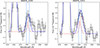 |
Fig. B.1. Spectral fits in the region around the [O III] λ4363 line that contains three emission lines (Hγ, [Fe II] λ4360, and [O III] λ4363) for galaxies 4195 (left panel) and 5014 (right panel). The overall fit is represented by the solid blue line, while the two Gaussian components centred at 4360 and 4364 Å are shown as dashed red lines. The fit demonstrates that a single Gaussian at 4364 Å alone cannot adequately reproduce the spectral features of these two galaxies. The inclusion of the [Fe II] component provides a significantly better fit. |
B.2. The case of MARTA_3942
Object 3942 presented unique challenges due to its extended nature and the presence of a contaminant near the end of the slit. To address these issues, we applied a local background subtraction technique, avoiding self-subtraction and recovering part of the flux from the second shutter while excluding the contaminated region at the slit’s edge. However, the use of local background subtraction inevitably introduced some noise into the continuum, as the outer shutters were integrated for less time than the central one. This resulted in a particularly noisy continuum around the auroral line [O III] 4363.
A significant issue arise when fitting this region with pPXF: the algorithm attempts to model stellar features around Hγ (4340 Å) but is actually fitting the noise, partially suppressing the [O III] 4363 line. Although this line is clearly distinguishable above the continuum, the pPXF fit underestimates its flux.
To mitigate this issue and recover a more accurate flux measurement, we subtracted the continuum modelled on the full three-nodding reduction version of the spectrum from the local background-subtracted spectrum. In this way, the model continuum was significantly smoother due to the more uniform exposure across the slit, but it was re-scaled to match the fiducial, local background-subtracted spectrum, before fitting the [O III]λ4363 emission line with an individual Gaussian component. The revised fit yields a line flux of 3.51 × 10⁻¹⁹ erg/s/cm2, recovering additional flux compared to the previous fit (3.11 × 10⁻¹⁹ erg/s/cm2).
B.3. Different continuum modelling
To assess the impact of the adopted continuum modelling on our derived quantities-particularly electron temperatures – we performed a set of tests using a variety of stellar population synthesis templates and polynomial corrections. Specifically, we repeated the spectral fits using several stellar libraries, including eMILES (Vazdekis et al. 2016), BC03 (Bruzual & Charlot 2003), CB07 (Charlot & Bruzual, unpublished), MILES-HC (a high-resolution subset of MILES; Conroy et al. 2018), and PEGASE (Le Borgne et al. 2004).
To directly quantify the influence of continuum modelling choices on key line measurements, we compared the fluxes of important emission lines – including [O III] λ4363 – across different template fits. As shown in Fig. B.2, which illustrates fits for a representative galaxy, the depth of Balmer absorption features can vary significantly depending on the chosen template (Belfiore et al. 2019). Nonetheless, the effect on the flux of [O III] λ4363 remains small, typically under ∼10%. The corresponding variation in the derived electron temperatures is generally within 10−15%, although we found that in galaxies with weaker auroral lines and lower S/N – such as MARTA_2387 – the inferred T3 can vary by up to ∼25%. Conversely, in cases with strong lines and high S/N, variations are as low as 2%.
For the Balmer lines used in the derivation of dust attenuation, we minimised the impact of template-dependent absorption differences by focusing on the strongest lines-Hα, Hβ, Hγ, and Hδ-whose high S/N ensures that absorption variations alter the measured fluxes by no more than ∼5%. Overall, these tests confirm that our continuum modelling approach is robust. Neither the choice of stellar template nor the polynomial order used for continuum correction introduces any systematic uncertainty that would affect the key conclusions ofthis work.
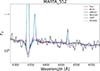 |
Fig. B.2. Example continuum fits for a representative object – MARTA_552 – using different stellar population synthesis templates. The figure illustrates the variation in the modelled absorption feature under the Hγ, and the corresponding stability of the [O III] λ4363 emission line flux. |
Appendix C: Different parametrisation of the T2-T3 diagram
We further analysed the T2-T3 relationship by comparing the temperatures derived for the MARTA sample with the multi-parametric calibration proposed by Yates et al. (2020). This approach is motivated by two primary considerations: (i) there is an anti-correlation between the electron temperature and the oxygen abundance. This means that if T([O III]) ≪ T([O II]), then it would be [O III] ≫ [O II], i.e. systems where the temperature of the doubly ionised oxygen is lower than the singly ionised oxygen one, tend to have a higher proportion of doubly ionised oxygen relative to singly ionised oxygen. In these cases, the total oxygen abundance Z(Te) becomes less sensitive to changes in Te([O III]). Conversely, systems where Te([O III]) > Te([O II]) exhibit the opposite pattern: the singly ionised oxygen fraction dominates, and the total oxygen abundance becomes less sensitive to Te([O III]). (ii) There is an empirical anti-correlation between Te([O III]) and Te([O II]) at fixed oxygen abundance. This is expected theoretically because an increase in the singly ionised oxygen fraction is balanced by a decrease in the doubly ionised oxygen fraction, andvice versa.
To model this, Yates et al. (2020) adopted a rectangular hyperbolic form centred at 0 K:
![Mathematical equation: $$ \begin{aligned} T_e([\mathrm{O}\,ii ]) = a(Z_{Te})^2 \frac{1}{T_e([\mathrm{O}\,iii ])}, \end{aligned} $$](/articles/aa/full_html/2025/11/aa54843-25/aa54843-25-eq12.gif) (C.1)
(C.1)
where a(ZTe) is a function depending on metallicity. Using this parametrisation, we examined how well the MARTA sample temperatures conform to the best-fit calibration of Yates et al. The results are presented in Fig. C.1: the main panel shows the T2-T3 relation colour-coded by the metallicity, revealing that for some galaxies, the interconnected dependence of T2, T3, and metallicity is well reproduced by the Yates calibration. This alignment is particularly evident in the continuous gradients of metallicity along the T2-T3 plane.
The inset panel quantifies the agreement by plotting ΔZ versus Z, where ΔZ represents the difference between the observed metallicity (calculated using the Te method) and the metallicity predicted by the Yates calibration, given the observed temperatures. Although some galaxies show good agreement (with ΔZ close to zero), for others significant deviations areapparent.
These discrepancies might arise because of the inapplicability of such a parametrisation to high-redshift galaxies, where the physical conditions of the ISM may deviate substantially from those in the local universe. For instance, at higher redshifts, ionisation parameters and density conditions can lead to deviations from the trends captured by the Yates calibration, necessitating further exploration of these dependences in different galactic environments.
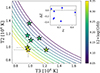 |
Fig. C.1. Parametrisation of the T2-T3 plane from Yates et al. (2020). MARTA galaxies are overplotted, colour-coded by their Te-based metallicity. The solid lines represent the T-T relation calibrated by Yates et al. (2020) for a fixed metallicity. Inset panel: ΔZ vs Z plot, where Z is the metallicity derived from the Te method for the MARTA objects and ΔZ is the difference between the ‘direct’ metallicity and that obtained from the Yates et al. (2020) calibration for the same galaxies. |
Appendix D: Emission line fluxes for MARTA galaxies
Table D.1 presents line fluxes, errors, and S/N estimates for all the auroral line detections in the MARTA gold and silver sample.
Fluxes, errors, and S/Ns of detected oxygen and sulphur auroral lines for each galaxy in the sample.
Appendix E: Representativeness of the auroral-line sample relative to the star-forming main sequence
To investigate the potential bias of the high-redshift auroral-line sample with respect to the star-forming main sequence, we examined the location of each galaxy in the SFR–M⋆ plane. Stellar masses and SFRs for the literature sample were taken from the original studies, without homogenisation. We then computed the offset from the MS, defined as ΔMS = log(SFR)−log(SFRMS), where SFRMS is the expected SFR at a given redshift and stellar mass according to the parametrisation by Popesso et al. (2023).
We find that the sample is, on average, significantly biased towards galaxies with elevated specific SFRs. The median offset across the full sample is ΔMS ≈ 0.7 dex. This is illustrated in Fig. E.1, where we show the SFR–M⋆ diagram for all galaxies used in the strong-line calibration, along with the MS relations at different redshifts from Popesso et al. (2023) and Morishita et al. (2024b). The offset is particularly pronounced at low stellar masses (M⋆ < 108.5 M⊙) and at high redshifts (z > 4), where only galaxies with the highest SFRs are typically detected in emission lines, and in particular show auroral lines.
To quantify this further, we split the sample by stellar mass and redshift. Galaxies with M⋆ < 108.5 M⊙ (N = 30) show a median ΔMS = 1.19 dex, while more massive galaxies (N = 53) have a lower median offset of 0.43 dex. Similarly, galaxies at 1 < z ≤ 4 (N = 29) have a median ΔMS = 0.42 dex, compared to 0.78 dex for those at z > 4 (N = 54). These trends reflect a combination of selection effects and the current limitations of deep spectroscopic observations at high redshifts.
The key concern is that a bias towards systems with high specific SFRs could correlate with the physical conditions in H II regions-particularly the ionisation parameter-and thus influence the derived strong-line calibrations. To address this, we examined the calibration diagrams shown in the main text (see Sect. 7), this time colour-coding each galaxy by its ΔMS. The result, shown in Fig. E.3, reveals no clear systematic trend or shift in the location of galaxies in strong-line ratio space as a function of ΔMS. While our sample is biased towards elevated specific SFRs, this does not appear to introduce a significant distortion in the empirical calibrations.
Nonetheless, we stress that this test is limited by sample size and the uncertainty on both the MS parametrisations and the reported SFRs. A more robust assessment would require a larger, statistically representative set of high-redshift galaxies with auroral-line detections, as well as an improved characterisation of the intrinsic scatter in line ratios at fixed metallicity. We defer a more detailed investigation to future work.
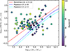 |
Fig. E.1. Locations of the literature sample galaxies used for strong-line calibrations in the SFR–M⋆ plane. Stellar masses and SFRs are taken directly from the original studies, without re-fitting. Coloured lines indicate the main sequence relations at different redshifts from Popesso et al. (2023) and Morishita et al. (2024b). |
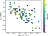 |
Fig. E.2. Offset from the main sequence of Popesso et al. (2023, ΔMS) as a function of stellar mass. |
Emission lines included in the fitting procedure.
All Tables
Physical properties of MARTA galaxies in the golden (top) and silver (bottom) samples.
Polynomial coefficients of the best fit for the strong-line metallicity diagnostics.
Median offset and dispersion (scatter) in line ratios at fixed O/H for each diagnostic and calibration considered in this work.
Fluxes, errors, and S/Ns of detected oxygen and sulphur auroral lines for each galaxy in the sample.
All Figures
|
Fig. 1. Comparison of strategies for background subtraction in NIRSpec/MSA observations. Left (red): Standard three-point nodding strategy, in which the galaxy is observed in three positions within the shutter, and the background for each position is estimated using the corresponding shutter exposures from the other two nods. Centre (blue): Nod2 strategy, a two-position scheme where only two out of the three available positions are used for the nodding procedure in order to use the shutters farthest from the galaxy as the background. Right (magenta): Local subtraction approach, which uses the outer shutters from the two off-source positions (indicated by the filled-in shutters) to estimate the sky background. In this method, the object signal is taken from the sum of all three nod positions (connected by dashed magenta lines), but no background is subtracted from the same shutters. As such, this method can be more sensitive to local systematics or background gradients. |
| In the text | |
|
Fig. 2. Star formation main sequence for the MARTA sample. Different shapes correspond to different priority classes, as described in Table 1, and different colours to the different samples: the golden sample is in orange (Sect. 4.2), the silver sample in grey (Sect. 4.3), and the rest of the galaxies in blue. For comparison, we plot the parametrisation of the star-forming main sequence at z ∼ 2.15 (median redshift of the full MARTA sample) by Popesso et al. (2023). |
| In the text | |
|
Fig. 3. Diagnostic diagrams for the MARTA galaxies analysed in this work. From left to right: Distribution of the combined golden and silver samples on the O32 vs R23, [O III]/Hβ vs [N II]/Hα, and [O III]/Hβ vs [S II]/Hα diagrams, colour-coded by galaxy redshift. The grey contours indicate the region populated by local galaxies from SDSS, with darker shades denoting higher densities. Red contours mark the distribution of galaxies from the MOSDEF survey (Kriek et al. 2015), whereas the orange curve is the fit to KBSS galaxies from Strom et al. (2017); both surveys target primarily z ∼ 2 − 3 systems. The dividing lines between star-forming galaxies, AGNs, and LINER galaxies from Kewley et al. (2001, 2013) and Kauffmann et al. (2003) in both the [N II]-BPT and [S II]-BPT diagrams are also drawn. Median error bars are not shown, as they are smaller than the symbol size and would not be visible in the plot; this is due to the fact that these are among the strongest lines, measured with very high S/Ns. |
| In the text | |
|
Fig. 4. Auroral emission lines detected in the MARTA golden sample. The panels show emission line fits of the [S II] λ4068,4076, [O III] λ4363, [S III] λ6312, and [O II] λ7320,7330 transitions, with their rest-frame wavelengths marked as dashed blue lines. We show the continuum-subtracted spectra in black, and the Gaussian emission-line fits in blue. In the case of [S III] λ6312, two single Gaussians are shown (dashed red lines), since the [S III] line is blended with the [O II] λ6300. |
| In the text | |
|
Fig. 5. Spectral fit for MARTA_4502, observed using grating G140M (left) and G235M (right). The black line represents the observed flux, the blue line the stellar continuum fit, and the red lines the emission-line Gaussian fits. In the bottom panels we show in grey the residuals from the fit, while the orange line represents the pipeline error estimates. The zoom-in panels at the top provide a more detailed view of specific spectral features: the auroral lines [S II] λ4068 and [O III] λ4363 (left) and the spectral range around the [O II] λλ7320,7330 auroral lines (right). |
| In the text | |
|
Fig. 6. [O III] λ4363 auroral emission line detected in the MARTA silver sample. The continuum-subtracted spectra are shown in black, with Gaussian emission-line fits overlaid in blue. The dashed light blue lines mark the rest-frame wavelength of the [O III]. |
| In the text | |
|
Fig. 7. Relation between T[O III] and T[O II] for the MARTA sample (gold hexagons), compared with various samples from the literature at low (grey dots) and high redshifts (from JWST archival data, orange triangles). The plot also shows the 1:1 relation (dashed blue line) and two empirical calibrations of the T2 − T3 relation, from Pilyugin et al. (2009, dashed purple line) and Garnett (1992, dashed magenta line). The red squares represent the median values of the entire sample, binned in T3, with uncertainties given by the standard deviation within each bin. The red line shows the best-fit relation derived in this work. |
| In the text | |
|
Fig. 8. Dependence of the T2 − T3 relationship on different physical properties. Top row: Individual data points. Bottom row: Corresponding hexagonal binning. The colour-coding indicates the three selected physical properties, computed as median values within each bin in the bottom panels: the [O III]/[O II] line ratio (left), the electron density ne (centre), and the softness parameter η (right). In the top panels, MARTA objects are shown as hexagons and low-redshift galaxies as circles. The plots also include the Pilyugin et al. (2009) relation, the Garnett (1992) relation, the 1:1 relation, and our best-fit model. The direction of maximum variation in the colour-coded quantity, determined by the gradient angle, is indicated by navy arrows, with the associated uncertainty shown for reference as light blue arrows. This provides a visual representation of how each parameter varies across the T2 − T3 plane. |
| In the text | |
|
Fig. 9. Left panel: T[S II]–T[O II] relation for MARTA objects, compared with extragalactic H II regions together with the empirical calibration by Méndez-Delgado et al. (2023b), based on local H II regions. Right panel: T[S III]–T[O III] relation for MARTA objects, along with local H II region data and two high-redshift galaxies with archival JWST data (Rogers et al. 2024; Welch et al. 2025). The plot also shows the calibrations from Garnett (1992) and Rogers et al. (2021). |
| In the text | |
|
Fig. 10. Nine different strong-line diagnostics comparing our MARTA data (striped hexagons for the golden sample, plain hexagons for the silver) with high-z literature samples (crosses) and a set of empirical calibrations. The data are colour-coded by redshift bin. The high-redshift data include strong-line calibration measurements from JWST surveys (D’Eugenio et al. 2024; Navarro-Carrera et al. 2024; Sanders et al. 2024; Schaerer et al. 2024; Arellano-Córdova et al. 2025; Curti et al. 2025b; Morishita et al. 2025; Napolitano et al. 2025; Scholte et al. 2025; Stiavelli et al. 2025; Topping et al. 2025b). The empirical calibration curves from the local Universe are from Maiolino et al. (2008), Bian et al. (2018), Curti et al. (2020a), and Nakajima et al. (2022), colour-coded in a dark colour palette (blue, purple, green), while the high-redshift-based calibrations from Sanders et al. (2024) and Chakraborty et al. (2025) are represented with a warm colour palette (yellow, orange, and red). Dashed lines denote extrapolations of the calibrations outside the regime where they have been calibrated. Our best-fit relations to the high-redshift dataset are shown in red. In most cases, a third-degree polynomial was used; for the N2 and R2 diagnostics, we adopted a linear fit, as there were no particular features that required a higher-order polynomial. Furthermore, in the |
| In the text | |
|
Fig. 11. Median offset of the strong-line calibrations analysed in this work relative to the high-z sample (z ∼ 1 − 9.5), computed in bins of metallicity. The bins have a width of 0.15 dex and are included only if they contain at least five objects. Each panel corresponds to a different diagnostic. The colour palette is the same as used in Fig. 10 to distinguish between low-z and high-z based calibrations, with markers also representing this division: stars for high-z and squares for z ∼ 0 based calibrations. |
| In the text | |
|
Fig. 12. Offsets in the log of the chosen line ratio at fixed O/H, representing the difference between the observed ratio and the value predicted by our best-fit calibrations. High-z JWST sample points are colour-coded by redshift to highlight potential trends. |
| In the text | |
|
Fig. B.1. Spectral fits in the region around the [O III] λ4363 line that contains three emission lines (Hγ, [Fe II] λ4360, and [O III] λ4363) for galaxies 4195 (left panel) and 5014 (right panel). The overall fit is represented by the solid blue line, while the two Gaussian components centred at 4360 and 4364 Å are shown as dashed red lines. The fit demonstrates that a single Gaussian at 4364 Å alone cannot adequately reproduce the spectral features of these two galaxies. The inclusion of the [Fe II] component provides a significantly better fit. |
| In the text | |
|
Fig. B.2. Example continuum fits for a representative object – MARTA_552 – using different stellar population synthesis templates. The figure illustrates the variation in the modelled absorption feature under the Hγ, and the corresponding stability of the [O III] λ4363 emission line flux. |
| In the text | |
|
Fig. C.1. Parametrisation of the T2-T3 plane from Yates et al. (2020). MARTA galaxies are overplotted, colour-coded by their Te-based metallicity. The solid lines represent the T-T relation calibrated by Yates et al. (2020) for a fixed metallicity. Inset panel: ΔZ vs Z plot, where Z is the metallicity derived from the Te method for the MARTA objects and ΔZ is the difference between the ‘direct’ metallicity and that obtained from the Yates et al. (2020) calibration for the same galaxies. |
| In the text | |
|
Fig. E.1. Locations of the literature sample galaxies used for strong-line calibrations in the SFR–M⋆ plane. Stellar masses and SFRs are taken directly from the original studies, without re-fitting. Coloured lines indicate the main sequence relations at different redshifts from Popesso et al. (2023) and Morishita et al. (2024b). |
| In the text | |
|
Fig. E.2. Offset from the main sequence of Popesso et al. (2023, ΔMS) as a function of stellar mass. |
| In the text | |
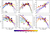 |
Fig. E.3. Strong-line calibration diagrams (see Sect. 7), with each galaxy colour-coded by its ΔMS. |
| In the text | |
Current usage metrics show cumulative count of Article Views (full-text article views including HTML views, PDF and ePub downloads, according to the available data) and Abstracts Views on Vision4Press platform.
Data correspond to usage on the plateform after 2015. The current usage metrics is available 48-96 hours after online publication and is updated daily on week days.
Initial download of the metrics may take a while.