| Issue |
A&A
Volume 703, November 2025
|
|
|---|---|---|
| Article Number | A176 | |
| Number of page(s) | 19 | |
| Section | Interstellar and circumstellar matter | |
| DOI | https://doi.org/10.1051/0004-6361/202555123 | |
| Published online | 13 November 2025 | |
Estimating the dense gas mass of molecular clouds using spatially unresolved 3mm line observations
1
Institut de Recherche en Astrophysique et Planétologie (IRAP), Université Paul Sabatier,
Toulouse cedex 4,
France
2
IRAM,
300 rue de la Piscine,
38406
Saint Martin d’Hères,
France
3
LUX, Observatoire de Paris, PSL Research University, CNRS, Sorbonne Universités,
75014
Paris,
France
4
Univ. Grenoble Alpes, Inria, CNRS, Grenoble INP, GIPSA-Lab,
Grenoble
38000,
France
5
Univ. Lille, CNRS, Centrale Lille, UMR 9189 - CRIStAL,
59651
Villeneuve d’Ascq,
France
6
LUX, Observatoire de Paris, PSL Research University, CNRS, Sorbonne Universités,
92190
Meudon,
France
7
Department of Earth, Environment, and Physics, Worcester State University,
Worcester,
MA
01602,
USA
8
Harvard-Smithsonian Center for Astrophysics,
60 Garden Street,
Cambridge,
MA,
02138,
USA
9
Department of Astronomy, University of Florida,
PO Box 112055,
Gainesville,
FL
32611,
USA
10
Instituto de Física Fundamental (CSIC).
Calle Serrano 121,
28006
Madrid,
Spain
11
Université de Toulon, Aix Marseille Univ, CNRS, IM2NP,
Toulon,
France
12
Max-Planck-Institut für Astronomie,
Königstuhl 17,
69117
Heidelberg,
Germany
13
Fakultät für Physik und Astronomie, Universität Heidelberg,
Im Neuenheimer Feld 226,
69120
Heidelberg,
Germany
14
National Radio Astronomy Observatory,
520 Edgemont Road,
Charlottesville,
VA
22903,
USA
15
Laboratoire d’Astrophysique de Bordeaux, Univ. Bordeaux, CNRS, B18N, Allee Geoffroy Saint-Hilaire,
33615
Pessac,
France
16
Instituto de Astrofísica, Pontificia Universidad Católica de Chile,
Av. Vicuña Mackenna 4860,
7820436
Macul,
Santiago,
Chile
17
Laboratoire de Physique de l’Ecole normale supérieure, ENS, Université PSL, CNRS, Sorbonne Université, Université de Paris, Sorbonne Paris Cité,
Paris,
France
18
Jet Propulsion Laboratory, California Institute of Technology,
4800 Oak Grove Drive,
Pasadena,
CA
91109,
USA
19
School of Physics and Astronomy, Cardiff University,
Queen’s buildings,
Cardiff
CF24 3AA,
UK
★ Corresponding author: This email address is being protected from spambots. You need JavaScript enabled to view it.
Received:
11
April
2025
Accepted:
27
August
2025
Abstract
Context. Emission lines such as HCN(J = 1 → 0) are commonly used by extragalactic studies to trace high density molecular gas (nH2 > ~ 104 cm−3). Recent Milky Way studies have challenged their utility as unambiguous dense gas tracers, suggesting that a large fraction of their emission in nearby clouds is excited in low density gas.
Aims. We aim to develop a new method to infer the sub-beam probability density function (PDF) of H2 column densities and the dense gas mass within molecular clouds using spatially unresolved observations of molecular emission lines in the 3 mm band.
Methods. We modelled spatially unresolved line integrated intensity measurements as the average of an emission function weighted by the sub-beam column density PDF. The emission function, which expresses the line integrated intensity as a function of the gas column density, is an empirical fit to high resolution (< 0.05 pc) multi-line observations of the Orion B molecular cloud. We assumed the column density PDF to be parametric, composed of a log-normal distribution at moderate column densities and a power-law distribution at higher column densities. To estimate the sub-beam column density PDF, we combined the emission model with a Bayesian inversion algorithm (implemented in the BEETROOTS code), which takes account of thermal noise and calibration errors.
Results. We validate our method by demonstrating that it recovers the true column density PDF of the Orion B cloud and reproduces the observed emission line integrated intensities within noise and calibration uncertainties. We applied the method to 12CO(J =1 → 0), 13CO(J =1 → 0), C18O(J =1 → 0), HCN(J =1 → 0), HCO+ ( J = 1 → 0) and N2H+(J =1 → 0) observations of a 700 × 700 pc2 field of view (FoV) in the nearby galaxy M51. On average, the model reproduces the observed intensities within 30%. The column density PDFs obtained for the spiral arm region within our test FoV are dominated by a power-law tail at high column densities, with slopes that are consistent with gravitational collapse. Outside the spiral arm, the column density PDFs are predominantly log-normal, consistent with supersonic isothermal turbulence setting the dynamical state of the molecular gas. We calculated the mass associated with the power-law tail of the column density PDFs and observe a strong, linear correlation between this mass and the 24 μm surface brightness.
Conclusions. Our method is a promising approach to infer the physical conditions within extragalactic molecular clouds using spectral line observations that are feasible with current millimetre facilities. Future work will extend the method to include additional physical parameters that are relevant for the dynamical state and star formation activity of molecular clouds.
Key words: ISM: clouds / ISM: general / ISM: lines and bands / galaxies: ISM / galaxies: star formation
© The Authors 2025
 Open Access article, published by EDP Sciences, under the terms of the Creative Commons Attribution License (https://creativecommons.org/licenses/by/4.0), which permits unrestricted use, distribution, and reproduction in any medium, provided the original work is properly cited.
This article is published in open access under the Subscribe to Open model. This email address is being protected from spambots. You need JavaScript enabled to view it. to support open access publication.
1 Introduction
Galactic studies show that star formation preferentially occurs in dense, gravitationally bound substructures within molecular clouds (e.g. Shu et al. 1987; André et al. 2010, and references therein). At parsec scales, this substructure is characterised by filaments that span several parsecs in length and have a characteristic width of ~0.1 pc (Arzoumanian et al. 2011). Once these filaments reach column densities of ~7 × 1021 cm−2, they become gravitationally unstable and tend to fragment into cores (André et al. 2014). The column density threshold for the formation of dense cores corresponds to an observational ‘dense gas’ threshold for local clouds, above which the rate of stars formed per dense gas mass is found to be constant (Lada et al. 2010). It has been proposed that the star formation rate (SFR) of a molecular cloud is set by the mass of gas above this threshold, while the mass of dense gas itself is set by the different physical mechanisms of filament formation. This cloud-scale picture of the relationship between the cloud substructure, gas column density distribution and star formation has largely been established from local cloud observations, where the spatial resolution is sufficient to characterise cloud substructures (e.g. Arzoumanian et al. 2011), the gas column density distribution (e.g. Schneider et al. 2013) and count individual young stellar objects (e.g. Lada et al. 2010).
Extragalactic observations offer the possibility to study star formation across a wider range of environments and physical conditions than encountered in local clouds. Focusing on the properties of dense (nH2 > ~104 cm−3) gas traced by HCN(J =1 → 0) emission, Gao & Solomon (2004) showed that there was a linear relationship between the infrared (IR) and HCN(J = 1 → 0) luminosities of 65 local galaxies, consistent with a cloud-scale SFR that is proportional to the dense gas mass if the HCN(J = 1 → 0) emission is a robust, universal tracer of high density gas. More recently, Gallagher et al. (2018b), Jiménez-Donaire et al. (2019) and Sánchez-García et al. (2022), have highlighted how the correlation between dense gas tracers such as HCN(J = 1 → 0) and the SFR varies within and among nearby (d < 20 Mpc) galaxies. Usero et al. (2015), Querejeta et al. (2019), Bešlić et al. (2021), Bešlić et al. (2024) and Neumann et al. (2023) have further shown that the HCN(J = 1 → 0)∕12CO(J = 1 → 0) ratio, considered to represent the fraction of high density molecular gas relative to the bulk molecular reservoir, varies with galactic environment (centre, bar, spiral arms, disc). Those studies find that the dense gas fraction is often enhanced in the central regions of galaxies, whereas the star formation efficiency in the dense gas (as traced by SFR∕HCN(J = 1 → 0)) decreases. The dense gas fraction and star formation efficiency have likewise been shown to vary with the cloud-scale molecular gas velocity dispersion and surface density (Gallagher et al. 2018a).
In practice, extragalactic observations suffer from limited spatial resolution and rely on a subset of bright lines arising from low-J rotational level transitions of molecules with high dipole moments. Such lines are commonly labelled ‘dense gas tracers’, which refers to their high critical density induced by the high dipole moment of their molecule. The conventional assumption is that HCN(J = 1 → 0), HCO+(J = 1 → 0) and other dense gas tracers emit predominantly at densities exceeding nH2 > 104 cm−3 (Gao & Solomon 2004). This ideal notion of the excitation of dense gas tracers has been challenged by recent high resolution observations of nearby Milky Way clouds (Pety et al. 2017; Barnes et al. 2020; Santa-Maria et al. 2023) and simulations of molecular clouds coupled to chemical networks and radiative transfer codes (Priestley et al. 2024). The growing understanding of these tracers is that a significant fraction of their cloud-scale emission can arise from gas at low to moderate densities where the lines are sub-critically excited. In this low density regime, for example, HCN(J = 1 → 0) sub-thermal excitation resulting from collisions with neutrals and electrons can produce faint emission across a spatially extended region (Goldsmith & Kauffmann 2017; Goicoechea et al. 2022), since the HCN(J = 1 → 0) abundance remains significant in diffuse, UV-illuminated regions (Santa-Maria et al. 2023; Liszt & Lucas 2001). This more nuanced perspective of the emission from HCN(J = 1 → 0) and similar species does not completely undermine their value as gas density tracers in external galaxies. In the absence of massive stars and widespread UV radiation, HCN(J = 1 → 0) excitation by electron collisions may be limited and contribute only a small fraction of the total emission measured over large spatial scales. Observationally, Jiménez-Donaire et al. (2023) have shown that the HCN(J =1 → 0) over N2H+(J = 1 → 0) ratio remains fairly constant at ~0.1-1 kpc scales in a galactic disc. Since the N2H+(J = 1 → 0) line has been observed to emit almost exclusively in dense, gravitationally unstable star-forming filaments and cores (Bergin & Tafalla 2007; Priestley et al. 2024), a constant HCN(J = 1 → 0) over N2H+ (J = 1 → 0) ratio tends to support the validity of HCN(J = 1 → 0) as an observational probe of dense gas. In summary, the caveats surrounding the use of HCN(J = 1 → 0) and similar lines as dense gas proxies call for better modelling of their spatially unresolved emission and methods that take into account that extragalactic measurements sample the emission arising from gas with a range of densities that are averaged within a single telescope beam.
This paper proposes such a ‘beam-averaged’ model in which the sub-beam distribution of column densities is expressed as a piecewise log-normal (LN) and power-law (PL) distribution (often referred to as a ‘gravoturbulent’ model in the literature, e.g. Burkhart 2018). Spatially unresolved integrated intensity is then an average of a sub-beam emission function weighted by the sub-beam column density PDF. Other studies have proposed a similar modelling approach in the past (Leroy et al. 2017; Bemis et al. 2024) but were mainly focused on a parametric study of their model. Here, we propose a full Bayesian inversion procedure to retrieve the PDF parameters from unresolved observations. Furthermore, the model presented here relies on an empirical emission function based on the multiline, high-resolution (<0.01 pc) ORION B survey, to account for both chemical and radiative transfer effects that have an impact on emission lines over several orders of magnitude in column density, whereas previous studies relied on RADEX-based radiative transfer modelling of each resolution element of the sub-beam volume density PDF. Thus, we consider the PDF of column densities (henceforth N-PDF) instead of volume density distributions (n-PDF).
The ORION B survey and other datasets used in this work are described in Section 2. The overall ‘beam-averaging’ model and the empirical emission function are presented in Section 3.1. The Bayesian inversion procedure, based on the work of Palud et al. (2023) and the code BEETROOTS, is summarised in Section 4. Section 5 presents a test of the inversion performance using the spatially averaged ORION B data, which we also use to explore the model’s degeneracies. In Section 6, we apply our inversion method to a 700×700 pc2 (14×14 pixel) field in the nearby galaxy M51, using 3 mm line observations from the SWAN survey (Stuber et al. 2025). Limitations and future improvement of the model, comparisons with other ‘beam unmixing’ techniques and comparison with the single dense gas tracer and line ratios approaches are discussed in Section 7. We summarise our key findings and conclusions in Section 8. Illustrations of the current model’s most important degeneracies (Appendix A), observations compared to model predictions in the Orion B cloud (Appendix B), maps of signal-to-noise and predicted line intensities in the M51 target region (Appendix C) and a parametric study of the model (Appendix D) are provided as appendices.
2 Data
2.1 Orion B data
We used data from the IRAM ORION-B (Outstanding RadioImaging of OrioN B, co-PIs: Pety & Gerin, Pety et al. 2017) Large Programme. The observations target a 18×13 pc region within the Orion B molecular cloud, a well-known star-forming region at a distance of 410 pc (Cao et al. 2023). ORION-B data surveyed frequencies from 72 to 116.5 GHz with a spectral resolution of 0.5 km s−1. The typical angular resolution of the observations is 25", corresponding to a linear resolution (beam size) of 0.05 pc, with data gridded on 9" (0.02pc) pixels. Depending on the observed frequency, the median noise level in the datacube ranges from 100 to 180 mK. A more comprehensive description of the ORION-B survey, including a description of the data acquisition and reduction procedures, is presented in Pety et al. (2017). In this paper, we used the nine strongest emission lines detected in the ORION-B dataset: 12CO( J =1 → 0), 13CO( J =1 → 0), C18O( J =1 → 0), HCO+( J =1 → 0), HCN( J =1 → 0), HNC(J =1 → 0), 12CS(J = 2 → 1), SO(Jκ = 32 → 21) and N2H+( J =1 → 0).
To complete the IRAM 30 m emission line data, we used column density maps presented by Lombardi et al. (2014). These column density maps are derived from dust far-infrared (FIR) and sub-millimetre continuum observations by the Herschel Gould Belt Survey (André et al. 2010; Schneider et al. 2013) and Planck satellite (Planck Collaboration I 2014). Through a fit of the spectral energy distributions constructed from these datasets, Lombardi et al. (2014) inferred the spatial distribution of the dust opacity at 850 μm (τ850). The opacity at 850 μm is converted to a visual extinction via Av = 2.7 × 10⁴ τ850 mag, as described in Pety et al. (2017). The H2 column density is then estimated from the visual extinction using the conversion factor NH2/AV = 0.5NHI/Av = 0.9 × 1021 cm−2 mag−1.
2.2 M51 data
We used observations of molecular line emission in M51 (distance = 8.58Mpc, McQuinn et al. 2016) from the SWAN (Stuber et al. 2025) and PAWS (Schinnerer et al. 2013) surveys. SWAN observed the 13CO(J =1 → 0), C18O(J = 1 → 0), HCO+( J = 1 → 0), HCN(J = 1 → 0), HNC( J = 1 → 0) and N2H+(J = 1 → 0) lines at an angular resolution of 3” and a spectral resolution of 10km s−1 across the central 5 × 7 kpc2 part of M51. PAWS provides complementary 12CO(J =1 → 0) observations, which were spatially and spectrally smoothed to match the resolution of the SWAN data.
We used publicly available Spitzer 24 μm observations of M51 as a proxy of embedded star formation activity. The Spitzer map that we use is presented in Dumas et al. (2011). The observations have been deconvolved with the HiRes algorithm (Backus et al. 2005) in order to achieve an angular resolution of 3" (140 pc).
3 Modelling spatially unresolved emission
3.1 Formulation of the problem
For spatially unresolved emission lines, the observed integrated intensity is an average of the sub-beam distribution of integrated intensities arising from the two-dimensional projection of the molecular gas onto the plane of the sky. Given a function f (θ) : RD → RL relating the sub-beam intensities to the sub-beam physical parameters θ ∈ RD, the relation between the observed integrated intensities of a set of L emission lines y = {y1, ...,yℓ, ...,yL} ∈ RL and the sub-beam density distribution of physical parameters p(θ) can be expressed as
 (1)
(1)
where η is the pixel area filling factor of the molecular gas, accounting for intensity dilution due to blank sky contributions if molecular emission is present only in a fraction of the pixel area. Here, the function f (θ) is known and can be highly complex, for instance a sophisticated model including chemistry, realistic cloud geometry and radiative transfer. The distribution p(θ) integrates to one by definition.
In general, this equation is impossible to invert, since the integration over an unknown multi-dimensional distribution makes it highly degenerate. To make the model invertible, the function f (θ) should be as simple as possible, focusing on the most sensitive variable θ. In this paper, the physical parameter of interest is NH2, which is also the parameter that predominantly drives the intensity of molecular emission lines (Gratier et al. 2017, 2021). Knowing this, the inversion problem can be greatly simplified by reducing the parameter space to NH2 only
 (2)
(2)
The contribution of other parameters to the emission is either considered to be negligible, or encoded in f (NH2). The main difficulty is to retrieve the continuous distribution pNH2 from a small (L<10) set of observations. This can be achieved by either discretizing the distribution into bins or assuming that the distribution can be parametrised with a small set of parameters φ. When discretising the distribution, the free parameters φ are the height of the individual bins, thus limiting the column density resolution that can be achieved to the number of independent observations. Since extragalactic millimetre surveys only target a handful of emission lines, we prefer to assume a parameterised form for p(NH2), ensuring that we have fewer parameters than independent observations and adopt physically motivated assumptions for the shape of the column density PDF.
3.2 Parametrisation of the gas column density distribution
To select the appropriate parametric family of distributions representing N -PDFs, we examine the shapes of N -PDFs determined from both numerical simulations and observations. In this section, we discuss how the shape of the column density PDF depends on turbulence and gravity, the dominant physical processes that, together with the magnetic field, determine the dynamical state of the molecular gas (Mac Low & Klessen 2004).
3.2.1 Isothermal supersonic turbulence
The volume and column density PDF of molecular and atomic gas depends largely on turbulence. Two common assumptions about turbulence in cold and dense ISM are that the gas is isothermal and the turbulent motions are supersonic (Larson 1981). An analytical prediction and consequence of supersonic isothermal turbulence is the parametrisation of the density PDF (whether volume or column density) as a LN (Vazquez-Semadeni 1994). This type of distribution has been observed in numerical simulations (e.g. Nordlund & Padoan 1999; Federrath et al. 2008) and confirmed by observations (e.g. Kainulainen et al. 2009). Qualitatively, a LN distribution naturally arises in a multiplicative stochastic process. Density fluctuations may be regarded as the result of a product of independent and identically distributed random variables (successive shock compressions). The log of these density variations then turns into a sum of random variables, which approaches a normal distribution under the central limit theorem. The column density distribution with mean N0 and standard deviation σ can then be expressed as
 (3)
(3)
where the expectation μ is related to the variance σ via μ = −σ2/2. This condition is mostly relevant for numerical simulation and imposed by mass conservation requirements in the closed box simulation (Nordlund & Padoan 1999). While μ = 0 could be used (e.g. Vazquez-Semadeni 1994) here, we still chose to impose the above relation between mean and variance in order to facilitate the comparison with numerical simulations.
3.2.2 Gravitational collapse
Turbulence is not the sole mechanism affecting the gas density distribution in molecular clouds. Gravity, as it becomes dominant over turbulence at higher gas densities, will tend to produce a PL tail with an index -α such that
 (4)
(4)
The emergence of a PL tail in volume and column density PDFs was first observed in numerical simulations (e.g. Slyz et al. 2005; Kritsuk et al. 2011; Federrath & Klessen 2013) and later detected in nearby molecular clouds (Kainulainen et al. 2009; Schneider et al. 2022). Such PL tails are generally attributed to gravitationally collapsing gas. Indeed, a collapsing homogeneous sphere of gas is expected to develop a radial profile of density ρ(r) = r−k (Shu 1977). As shown by Federrath & Klessen (2013), in this scenario the volume density PDF defined as p(ρ) ∝ dV/dρ becomes
 (5)
(5)
with V ∝ r3 the volume. For column densities, the radial density profile is N(r) ∝ ρr ∝ r−k + 1 and the distribution of column density becomes
 (6)
(6)
with A ∝ r2 the area. Relating Equations (4) and (6), the PL index α of the N-PDF can therefore be associated to an equivalent radial density profile of index k = (1 + α)/(α - 1). The analytical expectation for k in a collapsing isothermal sphere is 2 (corresponding to α = 3) in the outer static envelope of the collapsing sphere and 3/2 (α = 5) in the free-falling inner envelope (Shu 1977).
Arzoumanian et al. (2011) estimated the radial density profile of filamentary structures in the IC 5146 molecular cloud using Herschel observations. They reported indices k ∈ [1.5 : 2.5], equivalent to α = 2.3-5. In numerical simulations, Federrath & Klessen (2013) observed PL tails at higher densities, with values of k also ranging from 1.5 to 2.5. Across galactic molecular clouds, Schneider et al. (2022) observed PLs with slopes α ranging from 2 to 5.
3.3 Empirical emission function
In this paper, we use an empirically motivated emission function W (K km s−1) = f (NH2) that we obtain by fitting the ORION-B data. This choice is motivated by the need to capture not only the full complexity of emission lines’ excitation mechanisms, but also the chemical processes that alter molecular abundances. Indeed, the emission function must include several orders of magnitude in column density, covering both diffuse, illuminated regions and dense, well-shielded cores. The chemistry, and in particular photodissociation and molecular freeze out onto dust grains, must be accounted for, which is not the case for emission functions developed solely on radiative transfer calculations.
The choice of an empirical function is also partially motivated by recent observations of Milky Way clouds (Pety et al. 2017; Barnes et al. 2020; Tafalla et al. 2021, 2023) and numerical simulations (Priestley et al. 2024), which display similar emission functions even though the observed clouds harbour a wide range of star formation activity. The seemingly uniform behaviour of molecular line integrated intensities as a function of column density across nearby molecular clouds suggests that Galactic observations could be used to generate a calibrated emission function for extragalactic applications. Among available datasets, ORION B provides the best combination of high spatial resolution, sensitivity and broad frequency coverage over a cloud-scale field of view, hence its use as the basis for our empirical emission function.
In order to fit the relation between line integrated intensities and column densities, we binned the ORION B data in equally sized logarithmic bins of column density. In practice, we split the data in 30 bins, which we found to be a good compromise for establishing the average trend without excessively smoothing the variations. Figure 1 shows the resulting binned trend between column density and the integrated intensities of the emission lines that we include in our model, as well as the standard deviation in each bin.
For each emission line, the trend resembles a combination of two power laws with a smooth transition, which we fit using χ2 minimization of the following function:
![Mathematical equation: f_{\ell}(N_{\rm{H_2}}) = f_{l,b}\,\left( \frac{N_{\rm{H_2}}}{N_b} \right)^{\textcolor{black}{\beta_1}} \left\{ \frac{1}{2} \left[ 1 + \left( \frac{N_{\rm{H_2}}}{N_b} \right)^{\frac{1}{\Delta}} \right] \right\}^{\textcolor{black}{(\beta_2 - \beta_1)} \Delta}.](/articles/aa/full_html/2025/11/aa55123-25/aa55123-25-eq7.png) (7)
(7)
In this equation, Nb is the break location, β1 and β2 are the slopes before and after the break, ∆ is the smoothing parameter of the breaking point and fl,b is the function value at the break point. We discarded bins at lower column density with little or no data. The functions fl are specific to each of the l emission lines, and we summarise their fit parameters in Table E.1.
The scatter in the trends depends on the emission line considered. 12CO( J = 1 → 0) and 13CO(J = 1 → 0) show little scatter, whereas HCN(J = 1 → 0), HCO+ (J = 1 → 0) or 12CS(J = 2 → 1) display significantly larger dispersion. The dispersion around the mean trend increases with decreasing column density, which can be explained by the averaging of environments with varying radiation field. Indeed, the ORION B field of view displays a clear gradient of G0 from east to the west. Bins of lower column density corresponding to the outermost layers of the cloud can thus include diffuse and translucent regions with a wide range of UV-illumination.
A noticeable feature of these trends is the intensity of the 12CO(J = 1 → 0) line. It is significantly higher than the values observed by Tafalla et al. (2021) and Tafalla et al. (2023) in nearby clouds. The enhanced 12CO(J = 1 → 0) emission may be due to a higher gas temperature, driven by the high FUV radiation field pervading Orion B (Pety et al. 2017; Santa-Maria et al. 2023).
Besides radiative transfer and collisional excitation of the lines, Tafalla et al. (2023) explained the similarity of the trends they observed by transitions through different chemical regimes with increasing visual extinction. At column densities NH2 ≤ 12 × 1021 cm−2, the emission of CO molecules decreases sharply as the molecules in the surface layer of the cloud are photodissociated by the external radiation field. Above this column density threshold, shielding mostly prevents photodissociation and abundances remain relatively constant. The column density NH2 = 1-2 × 1022 cm−2 marks the transition to the ’freeze-out’ regime, where carbon molecules start to freeze onto dust grains. As a result, the abundances of C-bearing species steadily decrease as they are removed from the gas phase. Finally, column densities above NH2 = 1023 cm−2 are associated with regions dominated by stellar feedback. This regime sees increased emission from most species, in particular HCN(J = 1 → 0) and 12CS( J = 2 → 1), which is attributed to shocks and a substantial temperature increase affecting the chemistry of these molecules. The trends between line emission and column density described by Tafalla et al. (2023) are similar to what we observed in Orion B.
In conclusion, we adopt a realistic, albeit rigid, empirical emission function, which we constructed using a fit to the ORION B data. This implies that the method is applicable to regions where the metallicity, temperature, radiation and abundance are relatively similar to conditions in Orion B. Generalizing the emission function will be the subject of future work. We outline some caveats of the emission function and potential avenues to increase its flexibility in Section 7.2.
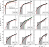 |
Fig. 1 Binned trends of line integrated intensity as a function of column density. The data are binned in 30 equally sized bins of column density. Black circles correspond to the bin average, while the grey shading indicates the standard deviation in each bin. The solid black line is a smoothly varying double PL fit to the trends, specific to each emission line. The dashed red line shows, for comparison, the empirical fit to the Perseus cloud by Tafalla et al. (2021), assuming a kinetic temperature of 11 K. Each panel shows a different emission line: 12CO(J = 1 → 0), 13CO(J = 1 → 0) and HCO+(J = 1 → 0) (left to right, top row); C18O(J =1 → 0), HCN(J =1 → 0) and 12CS(J = 2 → 1) (middle); HNC(J = 1 → 0), SO(JK = 32 → 21) and N2H+(J = 1 → 0) (bottom). The standard Milky Way CO-to-H2 conversion factor and its typical uncertainty (Bolatto et al. 2013) is indicated in the top left panel. An HCN( J = 1 → 0) dense gas conversion factor of 60 M⊙ (K km s−1)−1 is indicated in the central panel as the green curve. |
3.4 Global beam-mixing model
The final emission model reads
 (8)
(8)
with fℓ(NH2) given by Equation (7) and the parameters listed in Table E.1, while pφ(NH2) is defined as
 (9)
(9)
with C a normalisation constant and parameter p0 a constant ensuring continuity between the LN and PL segments. Its value is given by relating Equations (3) and (4) at NH2 = Nthresh. In practice, we express Nthresh as a function of N0 and μ as Nthresh = rthreshN0 exp(μ), to ensure that Nthresh < N0 exρ(μ). Similarly, we express α as a function of the parameter ![Mathematical equation: $d_\alpha = -\alpha / \left[ \frac{\diff{} \log( p{_{\rm{LN}}}(N_{\rm{H_2}}))}{\diff{} \log(N_{\rm{H_2}})}|_{N_\mathrm{thresh}} \right] < 1$](/articles/aa/full_html/2025/11/aa55123-25/aa55123-25-eq10.png) . This condition ensures that the PL tail is not steeper than the LN beyond the transition density Nthres In total, our model has five parameters φ = [N0, σ, rthresh, dα, η]. As there is no closed-form expression to Equation (8), the integral is computed numerically using the trapezoidal rule over a logarithmically spaced array of 100 column densities ranging from 1020 to 1024 cm−2. The constant C in Equation (9) is also computed numerically so that the N-PDF integrates to one.
. This condition ensures that the PL tail is not steeper than the LN beyond the transition density Nthres In total, our model has five parameters φ = [N0, σ, rthresh, dα, η]. As there is no closed-form expression to Equation (8), the integral is computed numerically using the trapezoidal rule over a logarithmically spaced array of 100 column densities ranging from 1020 to 1024 cm−2. The constant C in Equation (9) is also computed numerically so that the N-PDF integrates to one.
The LN width σ, the relative transition density rthresh and the PL index α could also be related as rthresh = (α - 1)σ2 if we impose a seamless transition between the LN and PL regime. This formulation removes one free parameter from the model. Along these lines, Burkhart (2018) and Burkhart & Mocz (2019) expressed the transition (volume) density as a function of α and σ, highlighting the transition density as the critical density for star formation and its relationship to the post-shock critical density for collapse (i.e. density at which the Jeans length is comparable to the sonic length). However, the N-PDFs of some local clouds display non-continuous LN to PL transitions. To give our model more flexibility, we thus chose to keep the transition density parameter free, which is why we refrain from referring to our LN + PL model as a ’gravoturbulent’ model.
It should be noted that the filling factor η introduced in this model is different from the standard line beam filling factor ηX. With our modelling approach,  , where X refers to the smallest column density for which the line is detected in the ORION B dataset. In other words, η is the filling factor of the gas whose column density is above NH2 > 1021 cm−2, whereas ηX is the filling factor of the considered line. In the ORION B dataset, the 1-σ sensitivity for the 12CO(J = 1 → 0) line is 0.3K km s−1 per pixel, which corresponds to a column density of 1021 cm−2 (see Figure 1). In this specific case,
  .
.
3.5 Average densities and dense gas fractions
Given the column density PDF pφ(NH2), a number of relevant molecular gas properties can be computed. The mass-weighted average surface density can be computed as
![Mathematical equation: \langle \Sigma \rangle \, = \int_{{-\infty}}^{+\infty} N_{\rm H_2} \, p_\phi(N_{\rm H_2}) \, dN_{\rm H_2}\modifr{.} \\[1em]](/articles/aa/full_html/2025/11/aa55123-25/aa55123-25-eq13.png) (10)
(10)
The mass-weighted average surface density of gas in the PL regime is
![Mathematical equation: \langle \Sigma_{\text{PL}} \rangle \, = \int_{N_{\text{thresh}}}^{+\infty} N_{\rm H_2} \, p_\phi(N_{\rm H_2}) \, dN_{\rm H_2}\modifr{.} \\[1em]](/articles/aa/full_html/2025/11/aa55123-25/aa55123-25-eq14.png) (11)
(11)
Finally, the mass-weighted average surface density of the ‘dense’ gas is similarly defined as
![Mathematical equation: \langle \Sigma_\text{dense} \rangle\, = \int_{\rm 10^{22}\,cm^{-2}}^{+\infty} N_{\rm H_2} \, p_\phi(N_{\rm H_2}) \, dN_{\rm H_2}, \\[1em]](/articles/aa/full_html/2025/11/aa55123-25/aa55123-25-eq15.png) (12)
(12)
where ‘dense’ refers to molecular gas at column densities above 1022 cm−2 to be consistent with Milky Way studies (Lada et al. 2010). These surface density quantities directly depend on the value of N0, which may be degenerated with the value of η (see Appendix A).
We also define quantities which are the product of surface densities with the filling factor η, and are thus unaffected by the potential degeneracy between N0 and η: total, dense and PL gas masses. The fractions of dense and PL gas can then be computed as  and
and  . Similarly, these quantities are unaffected by potential N0-η degeneracies.
3.6 Comparison with other unmixing approaches
Unmixing sub-beam physical and chemical parameters is a long-standing problem in astronomy and ISM studies. Several approaches have been developed to tackle this problem.
The most widely used model-free methods are inspired by or adapted from Earth observations methods of hyperspectral unmixing. The most commonly used of these methods is nonnegative matrix factorization, which blindly decomposes multi-spectral or hyperspectral observations into a linear combination of discrete independent components (referred to as end-members in the hyperspectral unmixing literature). These components can then be reliably attributed to specific environments, such as different dust grain populations (e.g. Berné et al. 2007; de Mijolla et al. 2024; Kishikawa et al. 2025).
Most methods nevertheless rely on physical models, whether numerical, analytical or empirical. These methods can be subdivided into two categories, depending on whether they assume a discrete or parametric sub-beam distribution of the physical parameters. For the discrete case, the methods used usually rely on one or two components (or zones) (e.g. Kaneko et al. 2023; Lizée et al. 2022; Ramambason et al. 2020; Vollmer et al. 2017). One-zone LTE or non-LTE modelling using a single set of average parameters (e.g. Roueff et al. 2021, 2024) would fit into this category. Methods relying on a high number of components have been developed, components which can even be divided in different sub-components (e.g. Ramambason et al. 2022). The alternative to the discrete case is to perform a parametric estimation of the sub-beam distribution of parameters. This requires prior knowledge on the shape of the distribution (characterised by a limited set of parameters) to be estimated. It is able to retrieve a complete, continuous distributions of physical properties with a minimum number of model parameters (e.g. Ramambason et al. 2024; Varese et al. 2025; Villa-Vélez et al. 2024). The method presented here falls into this last category.
In Earth observations, ‘unmixing’ traditionally refers to disentangling spatially averaged emission arising from specific environments. In astronomy, however, the mixing is threedimensional. Emission mixing along the line-of-sight becomes increasingly important compared to spatial averaging as the linear resolution of observations increases, to the point where the linear beam size is negligible relative to the observed gas length along the line-of-sight. Several methods have been specifically developed to perform line-of-sight unmixing. Ségal et al. (2024), for example, have recently proposed a discrete approach, modelling the gas structure using a three zone ‘sandwich’ model, that is two outer layers (a foreground and a background layer) surrounding an inner layer, with parameters to be determined in each layer. Our method could be extended to incorporate line-of-sight mixing by adapting Equation (1) to observables that are optically thin. In this case, our method could be used estimate the PDF of other parameters (e.g. the radiation field intensity G0) along sightlines of high linear resolution observations, once an appropriate emission function had been established.
4 Beam unmixing using Bayesian inversion
4.1 The Bayesian framework
Estimating the physical parameters of a system given a model and a set of observations is a common problem in astrophysics. Our problem is notably degenerate, since the observables arise from a sum over a PDF. Moreover, most of our observations have low to modest signal-to-noise ratios. We chose to solve it through a Bayesian framework to retrieve the distribution of solutions in the parameter space that is compatible with the observations, within noise and calibration uncertainties. Consequently, it can identify potential degeneracies in the solutions. The distribution of solutions π(Θ | Y) is called the ‘posterior distribution’, and is expressed by the Bayes’ theorem:
 (13)
(13)
The ‘prior distribution’ π(Θ) describes all a priori knowledge about the physical parameters that are to be estimated. This prior is coupled with the likelihood function π(Y | Θ), which gains more weight as information is provided, to produce the posterior distribution π(Θ | Y). The distribution π(Y) is a normalisation constant, the Bayesian evidence, which is not necessary to compute in Bayesian inference, hence the simplification of Equation (13). Once sampled, the posterior distribution can be used to compute different estimators of the ’best’ physical parameters describing the observations.
We used the method and the associated BEETROOTS1 code, described in detail by Palud et al. (2023). This method was specifically designed to retrieve model parameters from emission line observations, with a specific observational model including both noise and calibration uncertainties, and a sampling algorithm that efficiently samples the posterior distribution. Here, we summarise the main elements of the method, namely the noise model, prior information, sampling algorithm and estimators.
4.2 Observation and noise model
The noise model is a critical part of the Bayesian framework that describes how the different sources of noise degrade the observations, for instance through thermal noise and calibration errors. The observation model used in this work is, for a given pixel n:
 (14)
(14)
Here,  is a LN multiplicative noise expressing calibration errors, and
  is an additive Gaussian white noise associated to thermal noise. In this model, we assumed that
  and
and  are independent and their variances σm and σa are known.
4.3 Prior information
The prior distribution π(Θ) is another key element of the Bayesian inversion framework. This distribution encapsulates the prior information about the physical parameters to be estimated. In our case, there is no strong assumption about the parameters, aside from an expected range of acceptable values. Therefore, we use a uniform prior distribution on Θ (Jeffreys 1946), with the validity intervals listed in Table E.2. Given that all parameters range several orders of magnitude, we set their prior distribution to be uniform in log scale.
4.4 Sampling
In the case where the posterior distribution has no analytical formulation, Monte Carlo methods become necessary. In Bayesian inference, Markov chain Monte Carlo (MCMC) algorithms are the most widely employed Monte Carlo technique.
The model presented here is non-linear, which implies potential local minima, and must be inverted over large (> 10000 pixel) maps. These challenges are met by the specific MCMC algorithm implemented in BEETROOTS. This algorithm combines two complementary sampling kernels: the multiple-try Metropolis kernel (MTM) and the preconditioned Metropolis-adjusted Langevin algorithm (P-MALA). The MTM kernel facilitates a global exploration of the parameter space and escape from local minima, while the P-MALA samples the posterior PDF in and around the local minima. The combined ‘global’ and ‘local’ exploration of these kernels allows us to efficiently sample the posterior PDF. A complete description of the MTM and P-MALA kernels used in BEETROOTS is presented in Palud et al. (2023).
4.5 Estimators and uncertainty intervals
Different estimators of the parameters can be calculated from the posterior distribution, each with their own merits and drawbacks.
Here we use the Maximum A Posteriori (MAP) estimator, which maximizes the posterior distribution:
![Mathematical equation: \widehat{\Theta}_{\text{MAP}} = \underset{\Theta}{\arg\min} \, \left[ -\log \pi(Y \mid \Theta) - \log \pi(\Theta) \right].](/articles/aa/full_html/2025/11/aa55123-25/aa55123-25-eq24.png) (15)
(15)
We prefer it to the more commonly used minimum mean square error (MMSE), which is given by the mean of the posterior distribution, as degeneracies in the model can lead to strongly skewed posterior PDFs.
Uncertainty intervals on the estimated parameters can be derived straightforwardly from the posterior PDF. Here, we use the 16-84% percentile range on a parameter’s posterior PDF to quantify its uncertainty.
5 Testing on the ORION B dataset
As an initial test, we applied the method to the ORION-B dataset itself. We spatially and spectrally averaged the entire datacubes (including noise pixels) to mimic unresolved line observations of a giant molecular cloud. We then used the resulting vector of integrated intensities to infer the N-PDF. We used the dust column density map derived by Lombardi et al. (2014) to compute the ‘true’ N-PDF of the resolved region. We adopted a direct χ2 fit to this column density distribution as our reference N-PDF. The aim of this test is to demonstrate the method’s ability to retrieve a non-ideal N-PDF, given a simple averaged emission function and noisy observations. We also use it to explore the degeneracies inherent to beam mixing.
We carried out the Bayesian inversion using the setup described in Section 4. We assumed a multiplicative error of 10%, which accounts for calibration uncertainties of the 30m/EMIR and NOEMA instruments. We estimated the additive error level from the ORION-B data cubes. For each spectrum, we computed the RMS noise level (σRMS) as the standard deviation of 220 signal-free channels. Since the input observations of the Bayesian inversion are integrated intensities, we propagated the estimated noise through the intensity integration to produce a map of the additive error level on the integrated intensities. We used the spatial average of the noise for each line as the additive error level. Both the optimisation and sampling processes ran for 10 000 iterations, which is enough to converge to a solution and fully sample the posterior PDF.
5.1 Method performance on ORION B
Figure 2 compares the true column density PDF, the χ2 fit that we use as a reference, the Bayesian MAP estimation and the individual N-PDFs computed from the MCMC samples. We summarise the parameters of the reference and Bayesian MAP estimated N -PDFs in Table B.1. The Bayesian MAP estimation from the 3 mm averaged line observations is in excellent agreement with the reference N-PDF over more than two orders of magnitude in column density. The main difference is the width σ of the LN which appears slightly underestimated compared to the true N-PDF. As pixels below NH2 = 1021 cm−α do not contribute to the total emission, the estimated N-PDF is slightly narrower, with a pixel area filling factor of 0.90 corresponding to the proportion of pixels with NH2 ≥ 1021 cm−2 in the ORION-B data. We quote the 16-84th percentiles of the MCMC N-PDF realisations as the uncertainty on each of the parameters. The dispersion among the MCMC N-PDFs is typically larger at low (NH2 < 2 × 1021 cm−2) and high (NH2 > 1022 cm−2) column densities.
Figure 3 shows the posterior distribution of the model parameters. The mean column density (N0) of the LN part of the distribution is the best constrained parameter with all sampled N-PDFs peaking around ~2.5 × 1021 cm−2. At densities above N0, all the MCMC N-PDFs are consistent with the reference N-PDF, although some sampled N-PDFs reproduce the PL part with a very large LN distribution.
More quantitatively, the Bayesian estimation  closely matches the reference value of N0 = 2.38 × 1021 cm−2. The PL index α is likewise tightly constrained and accurate, with an estimated value of
  , compared to the reference value of α = 3.19. The width (σ) of the LN part of the distribution is more uncertain,
  and slightly underestimate the reference value of σ=0.47. The column density of the transition from the LN to PL part is also uncertain, with
  , with a strong tail in the posterior PDF. The MAP estimation nonetheless closely matches the reference value of Nthres = 4.08 × 1021 cm−2. The pixel area filling factor is unbiased, with
  compared to the reference value η = 0.90, corresponding to the proportion of pixels with NH2 > 1021 cm−2 in ORION-B. The pixel area filling factor being a scaling parameter, its uncertainty is directly related to the multiplicative error standard deviation of 10%, which explains the wide posterior distribution of this parameter. In this high signal-to-noise ratio example, there is little to no degeneracy between N0 and η.
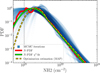 |
Fig. 2 Comparison of the reference and estimated N-PDFs when inverting the N-PDF on the spatially and spectrally averaged ORION-B data. The thick red line indicates the N-PDF as a histogram constructed directly from the dust-derived Orion B column densities, and the green line represents a χ2 fit to the red histogram. The estimated N-PDFs from the 10 000 MCMC iterations to sample the Bayesian posterior are shown with blue circles. The dashed orange line is the MAP estimation for the N-PDF. The vertical dotted black line indicates the limit below which the line intensities predicted by the emission function fall below the typical noise level of the data, that is, 0.1 K km s−1. |
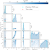 |
Fig. 3 Two-dimensional projections of the posterior PDF in the form of a scatter plot matrix. The matrix’s diagonal shows the posterior PDF of each estimated parameter. The MAP estimation is represented as a vertical cyan line on the histograms and as a cyan square in the scatter plot. The true N-PDF parameters obtained by fitting the dust-derived Orion B N -PDF are shown as red crosses. The dashed black line shows the range in PL index α of the N-PDF expected for gravitational collapse. The estimations closely match the reference values, although clear degeneracies are present in the posterior PDF. |
5.2 Method limitations
The wider posterior PDFs of α, σ and rthresh = Nthresh/N0 illustrate a loss of information inherent to beam-averaging, which limits the precision of the parameter estimation. Indeed, averaging the N-PDF produces two main effects on the model prediction and parameters. First, the method is subject to degeneracies, i.e. a co-variation of several parameters can lead to a similar N-PDF shape, and therefore yield similar emission line predictions. Second, the predicted intensities may lack sensitivity to a given parameter, due to the emission function that modulates the N-PDF that is then averaged to predict intensities. This occurs, for example, when a parameter primarily affects a part of the N-PDF where the emission function is negligible, such that the predicted intensities become insensitive to variations of this parameter. Alternatively, a large parameter variation might produce negligible variations in the N-PDF shape, and thus will not affect the predicted intensities. In this case, the fit procedure is also insensitive to the parameter. In Appendices D and A, we present a detailed study of these effects. In the rest of this subsection, we summarise the main caveats that we established from our inversion of the ORION-B dataset.
The most important caveat is that a co-variation of several parameters can yield an overall similar N-PDF shape. This scenario is visible in the joint posterior PDF of σ and rthresh, which displays a clear positive correlation. In this case, the PL tail is comparable to the LN distribution before the transition point Nthresh. Hence, a larger LN distribution with a larger Nthresh resembles a smaller LN distribution with a smaller Nthresh. Overall, the larger the LN distribution, the further away the transition to PL tail must be to preserve a similar shape. This results in the positive correlation between σ and rthres visible in Fig. 3. Figure A.2 illustrates this effect.
We further observe that compensation effects between the shapes of the N-PDF and the line emission function cause a “T” shape of the joint posterior PDF of α and σ. For σ values larger than the reference value, rthresh increases and so does the uncertainty on α, which causes the horizontal top spread of the joint posterior PDF. Indeed, as Nthres increases, the PL tail of the N-PDF becomes smaller. This in turn decreases the fraction of the beam-averaged emission sensitive to the PL tail to the point where the predicted intensities are no longer sensitive to the α parameter. This is illustrated in Figs. A.3 and D.2.
For σ values lower than the reference, the PL tail dominates and the LN width σ becomes unconstrained, which produces the vertical spread. Orion B’s N-PDF exhibits a strong PL component, which is visible even at low Nthres = 4.08 × 1021 cm−2 relative to N0 = 2.38 × 1021 cm−2. As a result, variations of σ mostly affect column densities below −1 × 1021 cm−2, where emission from all lines is below the noise level. Consequently, σ is poorly constrained and its posterior PDF is dominated by the uniform prior. This effect is illustrated in Fig. A.1. There is, however, a clear break in the posterior PDF at σ = 1 even though the validity interval goes up to σ = 2. We attribute this to our transition slope criterion: a σ value greater than one would result in a tangent at the transition flatter than the PL index α of Orion B, violating the slope criterion that we impose.
6 Application to M51 observations
The Surveying the Whirlpool at Arcseconds with NOEMA (SWAN) survey (Stuber et al. 2025) is a 3 mm line survey of the M51 galaxy over a 5 × 7 kpc FoV at 140 pc resolution (pixel size of 45 pc). The dataset includes high sensitivity observations of N2H+(J =1 → 0), as well as 13CO(J =1 → 0), C18O(J =1 → 0), HCN(J =1 → 0), HNC(J =1 → 0) and HCO+ (J =1 → 0). Here, we analyse a 700 × 700 pc region within the SWAN FoV centred on M51’s inner western spiral arm. The spiral arm crosses our test region from the north-east to the south-west (see Figure C.1). The signal from many lines is faint outside the arm, except for a patch of brighter emission in the north-west corner. We used the same setup for the Bayesian inversion procedure as for our test on the ORION-B data.
6.1 Spatial distribution of the N-PDF parameters
Figure 4 displays the spatial distribution of the estimated parameters: the mean of the LN part (N0), the pixel area filling factor (η), the average density including blank sky contributions, the width (σ), the location of the LN to PL transition (Nthresh) and the PL index (α). White pixels represent lines of sight where the integrated intensity is negative for at least one of the observed lines. Overall, there is clear spatial structure in the N-PDF parameter maps of our test region, with a transition from strong, high density PL tails in the spiral arm to lower density, mostly LN N-PDFs outside the arm. Some of the pixels adjacent to the white pixels show a pronounced PL tail, but the S/N is low at these positions and the fitted parameters are quite uncertain.
More quantitatively, the LN mean column density appears relatively constant accross the FoV at N0 ~ 1022 cm−2, with the exception of lower N0 values west of the spiral arm and higher values in low S/N regions. These higher N0 values coupled with very low pixel area filling factors are due to a level of degeneracy between N0 and η arising in low S/N pixels, as described in Appendix A. The pixel area filling factor on the other hand displays sharp contrasts, going from unity in the spiral arm to −0.1 outside. The average column density including blank contributions (i.e. (Σ) × η) is consistent with the observed 12 CO( J =1 → 0) emission. This average column density is enhanced in the spiral arm, reaching up to a few 1022cm−2, and rather uniform outside, with N0 ~ 5 × 1021 cm−2 on average and down to 1021 cm−2. The Nthresh distribution is bimodal, with (Nthresh ~ 2 × N0) in the spiral arm, and Nthresh ≥ 100 N0 outside. This reflects the presence and decay of the PL tail, inside and outside the spiral arm, respectively. The PL index is rather constant and within the [2,4] interval expected for gravitational collapse inside the spiral arm. We observe a slight flattening of the PL from inside to outside of the spiral arm. We consider the α values estimated outside the spiral arm region to be unreliable since the N-PDFs are mostly LN. The LN width σ is moderate in the spiral arm, broadly consistent with Milky Way cloud values (σ ~ 0.5, e.g. Schneider et al. 2022). Except for low S/N pixels, the highest σ values are associated with low N0 values, located in the north-western part of the FoV. This combination of high σ and low N0 effectively produces a low emission area filling factor, that is most of the N-PDF is below the threshold for 12CO(J = 1 → 0) emission, hence consistent with atomic or diffuse, CO-dark partially molecular gas, even though the pixel area filling factor is close to unity. The north-eastern part of the FoV displays the lowest N-PDF widths, with σ ~ 0.1, hinting that turbulence might be lowly supersonic or lowly compressive.
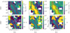 |
Fig. 4 MAP estimations of the sub-beam N-PDF parameters across our M51 test region. Top, from left to right : mean column density of the LN part of N-PDF (N0 ), the pixel area filling factor (η) and the average gas density (including blank sky contributions). Bottom : width of the LN (σ), the column density of transition between the LN and PL parts of the N-PDF (Nthresh) and the PL index (α). Red contours in each panel indicate 13CO(J = 1 → 0) integrated intensities of 4 and 12 K km s−1 (dashed and solid contours, respectively). The white arrow indicates the direction to the galactic centre. To first order, the gas is denser and more gravitationally unstable inside the spiral arm than outside it. |
6.2 Spatial distribution of dense gas
Figure 5 compares the spatial distribution of the dense gas mass, PL gas mass and 24 μm emission, which we use as a proxy for star formation. The dense and PL gas mass are computed from the estimated N-PDF parameters following the equations presented in Section 3.5, and adopting a distance to M51 of d = 8.58 Mpc.
The spatial distributions of dense and PL gas mass are similar. The mass is up to 10 times larger inside the spiral arm compared to regions outside the arm. A concentrated region of higher masses is visible in the centre of the arm, while moderately high dense gas masses are present in the south-western part of the spiral arm. For pixels outside the arm, there is little to no mass in the dense or PL regime. The transition from LN to PL occurs around −2 × 1022 cm−2, which is slightly higher than the critical density of filaments (NH2 = 7 × 1021 cm−2) determined by André et al. (2014) and the dense gas threshold derived by Lada et al. (2010) over which the SFR is observed to be proportional to dense gas mass in local clouds. The PL gas mass map shows a slightly higher contrast than the dense gas mass map. In the north-east of our target region, where the emission is associated with LN N-PDFs, the dense (and PL) gas mass fraction is low, despite the bright emission associated with this region.
The pixels that are coincident with the peak of 24 μm emission in the spiral arm exhibit N-PDFs with a pronounced PL tail and a large dense gas mass fraction. We identify pixels with N-PDFs with α ∈ [2.5,5] (see Sect. 3.2.2), and fgrav > 25% as being susceptible to gravitational collapse. The first condition is a standard criterion (see Sect. 3.2.2), while the second condition ensures that the PL represents a large fraction of the total emission, and thus that the α, rthresh and, by extension, MPL estimates are reliable. We present this relationship more directly in Fig. 6, where we show the correlation between the 24 μm surface brightness and the dense and PL gas mass. We consider two subsets of the data, depending on whether a pixel exhibits an N-PDF consistent with gravitational collapse as defined above. Both the dense and the PL gas mass in the gravity-dominated pixels (red symbols) demonstrate a tight linear correlation with 24 μm surface brightness, with a correlation coefficient r ~ 0.8, whereas pixels that do not fulfill our criteria for gravitational collapse (greyscale symbols) show no such correlation. The intensities of individual emission lines such as HCN( J = 1 → 0) or N2H+ (J = 1 → 0) display weaker and flatter (r = 0.7, s = 0.6) correlations with the 24 μm surface brightness than the dense and PL gas mass.
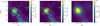 |
Fig. 5 Spatial distribution of the mass of dense gas (left), the gas mass in the PL part of the N-PDF (middle) and the 24 μm surface brightness in our M51 target region. We use the 24 μm emission as a proxy for star formation. The masses are derived from the MAP estimate of the N-PDF, using Eqs. (12) and (11). The red contours are the same as in Figure 4. The masses of dense and PL gas appear highly correlated, with a similar spatial distribution as the 24 μm emission. |
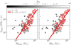 |
Fig. 6 Correlation between the 24 μm integrated intensity and: the mass of dense gas (left) and the mass of gas in the PL part of the N-PDF (right) for pixels within our M51 test region. Each data point corresponds to a pixel within our field. The symbol size and grey shading represent fPL, the mass fraction of the gas in the PL part of the N-PDF. Symbols with a red outline identify pixels where fPL ≥ 25% and the slope of the PL α ∈ [2.5,5]. The dotted line is a linear fit to the pixels where fPL < 5%. The thick red line is a fit to the points where fPL ≥ 25% and α ∈ [2.5,5]. The latter fit has a correlation coefficient r = 0.85 and slope s = 1.0. |
6.3 Interpretation
Our M 51 target region contains a spiral arm segment with bright 3 mm line emission, with fainter, more diffuse emission arising in the interarm region. The north-eastern corner of our field, i.e. the interarm pixels situated closest to the centre of M51, also exhibits moderately bright emission.
Our method delivers several interesting results. First, the spiral arm hosts the highest dense gas masses, up to Mdense = 106 M⊙. Second, the N-PDFs located in the spiral arm show average LN distributions (σ < 0.6), suggestive of supersonic turbulent gas with average Mach numbers, combined with pronounced PL tails with indices ranging from 2.5 to 4 consistent with gravitational collapse.
Third, pixels where a pronounced PL tail is present display a strong, approximately linear correlation between the dense and PL gas masses and the 24 μm emission, which we consider here as an embedded star formation tracer. Conversely, pixels devoid of PL tails show no such correlation. A linear correlation between dense gas mass and a star formation tracer is consistent with the hypothesis that the star formation efficiency is constant above a given column density threshold as observed in nearby Milky Way clouds (Lada et al. 2010).
Fourth, the transition from LN to PL inside the spiral arm occurs at a roughly constant column density, Nthresh ~ 2 × 1022 cm−2. This value is similar to the empirical dense gas threshold above which star formation is observed to be constant in nearby Milky Way clouds (Lada et al. 2010). Fifth, the inferred PL indices appear correlated with 24 μm emission, becoming steeper as the 24 μm surface brightness increases. This result is not entirely expected: regions with higher star formation activity should be associated with flatter PLs since the SFR is proportional to the available dense gas mass (Lada et al. 2010). In magnetohydrodynamical simulations without stellar feedback, Federrath & Klessen (2013) find that molecular clouds with flatter PL tails have a higher star formation efficiency (where SFE = M*/(Mcloud + M*). The trend that we observe could be the result of feedback mechanisms that are efficient in disrupting high density gas. In embedded regions, these mechanisms could preferentially act on gas with column densities corresponding to the PL tail of the PDF, steepening the PL.
Finally, outside the spiral arm, the N-PDFs are mostly LN, with smaller widths (σ < 0.3) than in the spiral arm. We interpret this as evidence that the molecular gas outside the arm is turbulence-dominated, lowly supersonic, and largely stable against gravitational collapse.
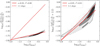 |
Fig. 7 Beam-averaged line ratios between HCN(J = 1 → 0) (left) and N2H+( J =1 → 0) (right) over 12CO( J =1 → 0) as a function of flense, for a sample of 100 000 N-PDFs with parameters uniformly sampled over N0 ∈ [5 × 10²⁰ : 1022], α ∈ [2.5 : 5], σ ∈ [0.2 : 1.3], and rthres ∈ [2 : 100]. The dashed red line shows a linear relation, while the solid red line shows a linear fit to the data. This parameter space is more limited than the validity intervals of Table E.2, but more representative of N-PDFs observed in local clouds (Schneider et al. 2022). |
7 Discussion
7.1 Comparison with the line ratio approach
To date, most studies of the dense molecular gas in external galaxies have relied on a line ratio approach. This approach can be likened to a two-zone model, with a low-density gas component, typically nH2 < 104.5 cm−2 (Gao & Solomon 2004), and a dense gas component at higher densities. The main assumption of the line ratio approach is that the emission of certain lines arise predominantly from the dense component (e.g. HCN(J = 1 → 0) Gao & Solomon 2004). Such lines are labelled as ‘dense gas tracers’. Emission lines such as 12CO(J = 1 → 0) that trace both low and high gas density components are regarded as ‘bulk gas’ tracers. Following these assumptions, combining observations of a bulk gas tracer and a dense gas tracer provides information about the dense gas fraction. By further assuming that these tracers vary linearly with the average density of the gas that they trace (i.e. assuming a constant αc0 or dense gas conversion factor), then the dense gas fraction simply becomes the ratio between the dense gas tracer and the bulk gas tracer. Attractive for its simplicity, this approach has been shown to be effective for the interpretation of extragalactic observations (see e.g. Schinnerer & Leroy 2024, Chapter 3, for a recent overview), where detecting a diverse suite of density-dependent emission lines is prohibitive with current observational facilities.
The method presented in this paper was designed to alleviate these shortcomings of the line ratio approach, leveraging the wide bandwidth, multi-line capacity of modern backends and recent observations revealing how the integrated line emission varies as a function of column density at high (~0.01 pc) resolution. For comparison, Figure 7 displays the HCN(J = 1 → 0) and N2H+ (J =1 → 0) ratios over 12CO(J =1 → 0) as a function of fdense for a sample of 100000 N-PDFs uniformly covering the parameter space. While the correlation between the HCN(J =1 → 0) over 12CO(J = 1 → 0) ratio and fdense is strong (Pearson correlation coefficient of r2 = 0.88), it is significantly sub-linear, with a correlation coefficient of m = 0.22. This is qualitatively consistent with the results of Bemis et al. (2024), and again demonstrates that the HCN(J = 1 → 0) over 12CO(J =1 → 0) ratio does not straightforwardly trace the fraction of gas above NH2 = 1022 cm−2. The significant contribution of low (NH2 < 1022 cm−2) density gas to the total HCN(J = 1 → 0) emission attenuates and flattens the correlation between dense gas mass and HCN(J = 1 → 0) emission (Leroy et al. 2017; Bemis et al. 2024).
On the other hand, the ratio between N2H+ ( J =1 → 0) emission and fdense is strong (r2 = 0.81) and almost linear (m = 0.84) over two orders of magnitude in line ratios and dense gas fraction. Thus, the ratio between N2H+ (J =1 → 0) and 12CO( J =1 → 0) appears to be a significantly better tracer of the dense gas fraction. The obvious practical drawback is that this diagnostic ratio requires robust detections of N2H+ (J = 1 → 0), which often implies prohibitive integration times for extragalactic sources.
7.2 Limitations and future improvements of the model
While they already give promising results, the parametrisations of the column density PDF and the emission function presented here are not universal and can be improved. The parametrisation of the N-PDF as a combination of a LN and a PL function, while both observationally and theoretically justified, assumes that the gas is isothermal. In the case of other polytropic indices, the (volume) density PDF can deviate from a pure LN, with for instance the development of a PL tail at low densities (Federrath & Banerjee 2015). Empirical studies likewise suggest that the N-PDF can display a bimodal profile, with a peak at high and low column densities (Schneider et al. 2022). The low column density peak, however, corresponds to atomic gas, thus below the column densities that we probed using molecular gas emission lines. In the extreme case where the turbulent forcing is strongly compressive, recent studies have shown that the volume density PDF differs from a LN distribution and instead resembles a Castaing-Hopkins PDF (Hennebelle et al. 2024; Brucy et al. 2024), especially if the Mach number is large (>20). The difference between the LN and Castaing-Hopkins shape is significant at high densities, with less dense gas in the Castaing-Hopkins PDF compared to the LN for a similar Mach number (Hennebelle et al. 2024). Investigating the characteristics of turbulence using other parametric density PDFs will be the subject of future work.
The emission function used for the analysis in this paper can also be improved. As an empirical law fitted on high quality data, our current emission function encapsulates the physics and chemistry relevant for molecular line emission across the range of column densities present in the ORION-B data. The drawback is the model’s lack of universality, making it most suitable for interpreting unresolved observations of regions where the gas properties are similar to those in Orion B. Variations in several potentially important physical parameters, such as the amplitude of turbulent gas motions and gas kinetic temperature, are not currently taken into account. The former could have a significant impact on the emission from optically thick lines such as 12CO(J = 1 → 0). Temperature variations, on the other hand, would mostly affect line emission arising from the outer layers of the cloud, e.g. 12CO(J =1 → 0) or 13CO(J =1 → 0). Emission lines such as N2H+ (J = 1 → 0) that are excited in the colder interior of the cloud should be less subject to temperature variations.
Beyond radiative transfer, chemical effects are also expected to influence the line emission, and could be incorporated into our emission model to some extent. For example, the photodissociation front of the cloud is expected to vary depending on the gas-phase metallicity and radiation field illuminating the molecular gas (Kaufman et al. 1999). A deeper front would globally shift the emission function displayed in Figure 1 to the right, progressively decreasing the emission from lower (12CO(J =1 → 0)) to higher (N2H+ (J =1 → 0)) density lines.
Similarly, a higher temperature or stronger radiation field pervading deeper into the cloud could shift the freeze out of molecules onto dust grains to higher column densities. A higher or lower column or volume density threshold for freeze-out of carbonated molecules would then significantly alter the emission function of N2H+(J = 1 → 0). Furthermore, FUV radiation can enhance the formation of HCN as well as increase the ionization fraction (Santa-Maria et al. 2023). The HCN molecules can then be significantly excited by e− collisions. These effects can produce low-level, extended HCN(J =1 → 0) emission in diffuse, illuminated gas. Averaged over an entire cloud, this emission arising from lower density (nH2 < 104 cm−3) gas can account for more than half of the total HCN(J = 1 → 0) (SantaMaria et al. 2023). Cosmic rays and their ionization rates are another key parameter left out of the equation for now. They play a major role in the intricate chemical network regulating the abundances of complex molecules. For instance, regions exposed to elevated ionizing rates such as galactic nuclei can display extended and overabundant N2H+(J =1 → 0) emission (Santa-Maria et al. 2021) compared to Orion B. Finally, stellar nucleosynthesis of carbon and oxygen isotope can change the relative abundances of CO isotopologues. 12C and 16O isotopes are preferentially produced in massive, short lived stars, whereas 13C and 18O are produced in lower-mass, longer lived stars during a slower process. As the population of stars varies from mostly young, massive stars in the inner star-forming disc to older, lower mass stars in the outer disc, both 13CO(J =1 → 0) over 12CO(J =1 → 0) and C18O(J =1 → 0) over 12CO(J =1 → 0) are expected to increase as a function of galactocentric radius (Wilson & Rood 1994).
The logical next step to develop our method would be to implement new physical parameters in the emission function. This would make the model more flexible while retaining its empirical motivation and permitting benchmarks against high resolution observations. There are several avenues that could be explored to implement new parameters: (1) discretizing the emission model into several one-zone models for specific parameters (e.g. an inner and outer cloud temperature, (see e.g. Ségal et al. 2024), (2) defining profiles of relevant parameters as a function of the column (or volume) density (e.g. Tafalla et al. 2021), or (3) a combination of the two previous approaches. A straightforward extension of the current model would be to impose a specific temperature corresponding to the cloud’s surface for optically thick tracers (e.g. 12CO(J =1 → 0)), and a temperature profile as a function of column density for emission lines that are excited in the colder and denser parts of the cloud.
An alternative way to improve the emission function would be to express the average intensity as a function of a twodimensional PDF of column density and temperature (or other relevant parameter). However, this would also require the twodimensional PDF to be parametric and quickly increase the number of parameters to be estimated. For instance, a temperature PDF composed of a combination of PLs would introduce three additional parameters to be estimated by the inversion.
In all of the above cases, the improvement of the emission function requires adding parameters. The main obstacle towards implementing this increase of physical parameters remains the limited number of emission lines that are accessible to observations of typical extragalactic star-forming regions. The number of independent observations must be larger than the number of parameters for the model to be invertible and to alleviate degeneracies. Additionally, the observed emission lines should be sensitive to the different physical parameters. To include more radiative transfer parameters, such as temperature, opacity, or even abundance variations, the natural next step would be to add higher order J-lines. The theoretical maximum level of information that an observable can deliver about a physical parameter can be quantitatively estimated using the mutual information measurement (Cover & Thomas 2006, Sect. 8.6). This metric is particularly well-suited to informing the selection of lines depending on the physical parameters of interest, as shown by Einig et al. (2024), and we encourage its wider use for observation planning.
8 Summary and conclusions
This paper presents a new method to infer the column density PDF and gas mass above a column density threshold from a set of spatially unresolved 3 mm emission line observations. The method assumes that the column density PDF can be parametrised as a combination of a LN distribution due to supersonic isothermal turbulence, and a PL distribution at higher densities, the latter arising from gravitationally unstable or collapsing structures. It also assumes that the intensity of the observed 3 mm emission lines mostly depend on the column density. The emissivity of each line is calibrated on the ORION-B data.
For validation, we applied the method to the spatially and spectrally averaged ORION-B data for nine emission lines. In this case, the method accurately recovers the column density PDF of the resolved data, and the model reproduces the integrated intensities of the input emission lines within noise and calibration uncertainties. We then applied the method to 3mm line observations towards a 700 × 700 pc field covering a spiral arm segment in the M51 galaxy from the SWAN Large Programme. The main results of our analysis of this region are the following:
The model reproduces the observed integrated intensities within 25% on average. With our current model, the predicted integrated intensities of the 13CO(J =1 → 0) and C18O(J =1 → 0) lines for some pixels show the largest discrepancy (up to a factor of two) with the SWAN observations.
Power laws of N-PDFs, consistent with gravitational collapse, are detected almost exclusively in the spiral arm region that crosses our M51 field. Outside the spiral arm, the N-PDFs are predominantly LN, with a small width, which is consistent with lowly supersonic or lowly compressive turbulence dominating the gas dynamics.
The relationship between the inferred dense gas mass and the 24 μm emission varies as a function of the N-PDF properties. There is no correlation between these quantities for purely LN N-PDFs, while a strong, almost linear correlation is present for N-PDFs with a significant PL component. The correlation steepens from null to linear as the fraction of gas mass in the PL increases from ≤5% to ≥25%.
The correlation between the 24 μm emission and inferred gas mass in the PL of the N-PDF is closer to linear and tighter than the correlation with the integrated intensities of individual emission lines. When the fraction of gas in the PL is greater than 25%, we find a correlation coefficient r = 0.85 and slope s = 1. Correlations with the integrated intensities of both HCN( J =1 → 0) and N2H+( J = 1 → 0) display weaker correlation coefficients (r ~ 0.7) and flatter slopes (s ~ 0.6).
Efforts to expand the current study are already underway. We are working to improve the emission function to include additional physical effects such as variations in the kinetic temperature and line width by developing the modelling strategies presented in Section 7.2. The application of this improved model to the full SWAN dataset for M51 will be presented in a future paper (Zakardjian et al, in prep.).
Acknowledgements
This work is based on observations carried out under project numbers 019-13, 022-14, 145-14, 122-15, 018-16 and finally the large programme number 124-16 with the IRAM 30m telescope and large programme number M19AA with the NOEMA interferometer. IRAM is supported by INSU/CNRS (France), MPG (Germany) and IGN (Spain). This research has also made use of data from the Herschel Gould Belt Survey (HGBS) project (http://gouldbelt-herschel.cea.fr). This work received support from the French Agence Nationale de la Recherche through the DAOISM grant ANR-21-CE31-0010, and from the Programme National ’Physique et Chimie du Milieu Interstellaire’ (PCMI) of CNRS/INSU with INC/INP, co-funded by CEA and CNES. M.G.S.M. and J.R.G. thank the Spanish MICINN for funding support under grant PID2019-106110GB-I00. M.G.S.M acknowledges support from the NSF under grant CAREER 2142300. Part of the research was carried out at the Jet Propulsion Laboratory, California Institute of Technology, under a contract with the National Aeronautics and Space Administration (80NM0018D0004). D.C.L. acknowledges financial support from the National Aeronautics and Space Administration (NASA) Astrophysics Data Analysis Program (ADAP).
Appendix A Example model degeneracies
This section provides examples of common ’beam-averaging’ degeneracies, illustrating how N-PDFs with distinct parameters can yield similar average integrated intensities.
Figure A.1 depicts a degeneracy on σ, which arises if the N-PDF is predominantly PL-like and centred at relatively low column densities (NH2 < 5 × 1021 cm−2. In this case, similar to Orion B in Section 5, changing the LN width only affects the N-PDF where the emission function is almost null. The average integrated intensities are thus unaffected, which makes the σ parameter degenerate.
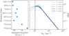 |
Fig. A.1 Left : model-predicted integrated intensities for a piecewise LN and PL N-PDF, with N0 = 2 × 1021 cm−2, rthres=1.5, α = 3 and σ increasing from 0.3 to 0.8. All predicted integrated intensities vary by 10% at most, which illustrates the degeneracy on the parameter σ in the particular case of low N0 and strong PL component. The right panel displays the corresponding N-PDF with varying σ. The dashed vertical line shows the column density limit below which the emission of all lines is less than 0.1 K km s−1 . |
Figure A.2 illustrates a degeneracy between σ and rthres, in the case where a co-variation of these parameters leads to a globally similar N-PDF shape, and therefore similar average integrated intensities. This kind of degeneracy appears as a correlation between σ and rthres in the posterior PDF of the Orion B Bayesian inversion in Section 5.
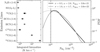 |
Fig. A.2 Same as Figure A.1, except two specific N-PDF are illustrated: the first has a narrow LN width but a strong PL, while the other has a large LN width but a smaller PL. This illustrates how two N-PDF with notably different parameters can appear alike and give comparable average integrated intensities. |
Figure A.3 displays a typical degeneracy on the PL parameters in the case where the PL accounts for a small fraction of the N-PDF, even though it covers high densities and so high values of the emission function. Here, varying α does not change the average line intensities. In other words, the PL parameters become intractable if rthres is high enough.
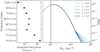 |
Fig. A.3 Same as Figure A.1, except the LN width is fixed to σ = 1 and the PL index is varying from 2 to 5. This illustrates the degeneracy on the parameter α when the PL appears far in the LN and therefore accounts for a negligible portion of the total N-PDF. |
Finally, figure A.4 illustrates the potential degeneracy between N0 and η. This figure shows 1) a set of N-PDFs with N0 and η are anti-varying over more than a factor of three, and all other parameters held constant, and 2) the corresponding predicted line integrated intensities. Overall, line integrated intensities vary by 5% at least (HCO+ (J =1 → 0)) to 50% at most (N2H+ (J = 1 → 0) and 12CO( J = 1 → 0)). While a predicted integrated intensity variation of 5% is insufficient to lift the degeneracy between η and N0 , a variation of 50% will break this degeneracy as this intensity variation is much larger than calibration uncertainties. However, this implies to well detect (at least) two lines sensitive to N0 and η, such as N2H+ (J = 1 → 0) and 12CO( J =1 → 0), which is consistent with peculiar N0 values towards the lowest S/N pixels in the FoV.
 |
Fig. A.4 Left : same as Figure A.1, except for N0 increasing from 3 × 1021 cm−2 to 1 × 1022 cm−2, η decreasing from 1 to 0.3 and σ = 0.3. The predicted integrated intensities vary by 10% to 50% at most (30% on average), which illustrates the degeneracy between the LN mean N0 and the pixel area filling factor η. The right panel displays the corresponding N-PDF with varying N0. |
Appendix B Observations versus model predictions in Orion B
Figure B.1 shows the posterior predictive distribution from the Bayesian inversion on the Orion B data performed in Section 5. The model prediction for the estimated parameters (MAP) matches the observed line intensities, and both the model best prediction and observations sit well within the distribution of prediction from the entire posterior PDF, with no visible offset.
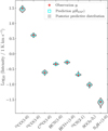 |
Fig. B.1 Posterior predictive distribution from the Bayesian inversion on the Orion B data performed in Section 5. The red crosses show the observed intensity, the cyan squares show the model prediction for the MAP estimator and the grey violin plot shows the histogram of model predictions for the entire posterior PDF (every MCMC iteration). |
Orion-B N-PDF parameters estimated from χ2 fitting of the dust-derived column density map compared to the Bayesian inversion (MAP estimation) results.
Appendix C Observations versus model predictions in M51
Figure C.1 compares the model predictions to the observations across our M51 test region. The 12CO(J =1 → 0) and HCO+(J = 1 → 0) integrated intensities are well-reproduced by the model, with an intensity weighted average prediction over observation ratio of 0.95 and 0.96, respectively. On one hand, the HCN( J = 1 → 0) and HNC( J = 1 → 0) integrated intensities are slightly underestimated, with average ratios of respectively 0.86 and 0.89. And the C18O(J = 1 → 0) emission is noticeably underestimated by the model, with an average ratio of 0.72. On the other hand, the 13CO(J = 1 → 0) N2H+ (J = 1 → 0) intensities are consistently over-estimated by respectively ~70% and ~50% on average.
For most emission lines, a clear spatial pattern is visible in the residuals, with over-estimation of the line intensities in the arm and under-estimation outside, or vice versa. Such a clear spatial pattern suggests local variations in the emission function, potentially caused by temperature, isotopologue abundance or opacity variations, as discussed in Section 7.2.
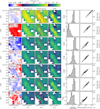 |
Fig. C.1 From the leftmost to the rightmost column: ratio of best model prediction over observed integrated intensities (in log10 scale, the colour scale limits are a factor of two in red and a factor 0.5 in blue), best model predictions, observations, S/N level, histograms of the residuals normalised by the observations and finally best model prediction as a function of observations. For the observation column, red contours in each panel indicate 13CO(J = 1 → 0) integrated intensities of 4 and 12 K km s−1 (dashed and solid contours, respectively). Each row is a different emission line, from top to bottom: 12CO(J = 1 → 0), 13CO(J = 1 → 0), C18O(J = 1 → 0), HCO+(J = 1 → 0), HNC(J = 1 → 0), HCN(J = 1 → 0) and N2H+(J = 1 → 0). |
Appendix D Parametric study of the model
This section describes the model predictions and its potential degeneracies in terms of line ratio variations over two-dimensional projections of the parameter space. Here and in the following section, the term line ratios refers to the predicted integrated intensity of different lines relative to the integrated intensity of 12CO( J = 1 → 0).
Appendix D.1 LN: line ratio variations with N0 & σ
Figure D.1 displays the line ratio variations as a function of N0 and σ. For this grid of predictions, the distribution is purely LN, with N0 varying from 1021 to 5 × 1022 cm−2 while σ increases from 0.2 to 1.8.
As expected, the parameter N0 has the most impact on the observed line ratios. Its increase shifts the entire N-PDF to higher density values where the emission function predicts stronger intensities, while the overall N-PDF shape remains unchanged. As 12CO(J = 1 → 0) emission quickly saturates, all line ratios increase with N0. These line ratio variations with respect to N0 range from one to four orders of magnitude, depending on the line considered. Emission lines for which the emission function flattens, or even saturates, at high NH2 show less variation (e.g. 13CO(J = 1 → 0)) than lines with steeper emission functions (e.g. 12CS(J = 2 → 1) or N2H+ (J =1 → 0)).
Variations in the line ratios due to σ are less pronounced, and mostly discernible for lower values of N0. Indeed, in this case, increasing σ will make the N-PDF sample progressively larger densities, increasing the line ratio values. However, if the N0 value is high enough - that is, the entire N-PDF is centred on higher densities (NH2 > 1022 cm−2 - then increasing σ induces less variation of the line ratios. This is because the emission functions of the different lines are significantly flatter at higher column densities. The increased degeneracy of σ as N0 increases is visible in Figure D.1 as the ratio isocontours turning vertical, and is particularly pronounced for HCN(J = 1 → 0).
Overall, all the emission lines considered here vary strongly (by at least a factor of four and up to three orders of magnitude) with either σ or N0 increasing by roughly an order of magnitude. In other words, for a pure LN distribution, both these parameters can be straightforwardly estimated.
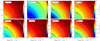 |
Fig. D.1 Model predicted line integrated intensities ratios over 12CO( J =1 → 0) as a function σ and N0 for a purely LN N-PDF. Top row shows the ratios of 13CO(J =1 → 0), HCO+ (J =1 → 0), HNC(J =1 → 0) and HCN( J =1 → 0) over 12CO(J =1 → 0), from left to right. In this top row dashed lines show ratio isocontours increasing by factors of two. Bottom row shows the ratios of12CS( J = 2 → 1), C18O( J = 1 → 0), SO(JK = 32 → 21 ) and N2H+ (J = 1 → 0) over 12CO(J = 1 → 0), from left to right. In the bottom row isocontours represent factors of tens. |
Appendix D.2 Power law: line ratio variations with Rthresh & α
Figure D.2 shows the line ratios as a function of rthres and α for a fixed LN distribution with N0 = 5 × 1021 cm−2 and σ = 0.6. α and rthres vary from 1 to 3 and 2 to 15, respectively.
Qualitatively, all line ratios behave similarly. Increasing either α or rthres brings the ratio values down. Increasing α steepens the PL part of the N-PDF, which reduces the range of higher densities covered and thus decreases the line ratios. Similarly, increasing rthres will push the transition from LN to PL further into the LN distribution, reducing the contribution of the high density PL to the N-PDF. Reducing the high density tail of the N-PDF consequently decreases the line ratios.
Quantitatively, there is overall little variation of the 13CO(J =1 → 0), C18O(J =1 → 0), HCO+ (J =1 → 0), HCN(J =1 → 0) and HNC(J = 1 → 0) ratios with rthres and α, with variations spanning less than an order of magnitude. Only SO(JK = 32 → 21)n 12CS(J = 2 → 1) and N2H+ (J = 1 → 0) line ratios over 12CO(J = 1 → 0) vary by more than an order of magnitude over the parameter space. The N2H+ (J = 1 → 0) over 12CO( J = 1 → 0) ratio in particular varies by more than two orders of magnitude and rather uniformly across the entire parameter space considered here. This makes N2H+ (J = 1 → 0) the best tracer to estimate PL parameters.
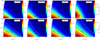 |
Fig. D.2 Same as Figure D.1, except that the N-PDF is composed of a LN and a PL, with varying rthres and α while σ and N0 are fixed to N0 = 5 × 1022 cm−2 and σ = 0.6. |
Appendix D.3 Potential degeneracy: line ratio variations with Rthresh & σ
Figure D.3 shows the line ratios as a function of rthres and σ, for a fixed LN mean value of N0 = 5 × 1021 cm−2 and a fixed PL slope α = 2.5.
The rthres parameter is notably degenerate. For rthres> 10, there is little to no variation of the line ratios with this parameter. As before, as rthres increases, the PL portion of N-PDF becomes negligible and its parameters become intractable. For rthres < 10, there is a degeneracy between σ and rthres, as shown by the isocontours curved pattern. This case of degeneracy is illustrated in Figure A.2. In the limit case where rthres <~ 2, the LN width parameter σ is degenerate. In this case the N-PDF is almost entirely PL, and the LN part of the N-PDF shapes lower densities only where the emission function is close to null. This type of degeneracy is illustrated in Figure A.1.
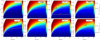 |
Fig. D.3 Same as Figure D.1, except that the N-PDF is composed of a LN and a PL, with varying rthres and σ while α and N0 are fixed to N0 = 5 × 1022 cm−2 and α = 2. |
Appendix D.4 Potential degeneracy: line ratio variations with α & σ
Figure D.4 shows the line ratios as a function of α and σ, for a fixed LN average value of N0 = 5×1021 cm−2 and a fixed rthres = 1.1.
The σ parameter is totally degenerate. This is caused by the rather low average density N0, combined with an early PL onset rthres = 1. In this case, the density distribution is dominated by the PL. Variations of σ result in variation of the PDF shape for NH2 < 1.1 N0; however, at these column densities the emission of lines is near 0, therefore variations of σ do not produce intensity variations.
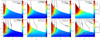 |
Fig. D.4 Same as Figure D.1, except that the N-PDF is composed of a LN and a PL, with varying σ and α while rthres and N0 are fixed to N0 = 5 × 1022 cm−2 and rthres=5. |
Appendix E Emission function parameters and validity intervals of the global emission model
Parameters of the smoothly broken PL function (Equation 7) fitted on the Orion B data through χ2 minimisation in Section 3.3.
Limits of the validity interval and prior distribution type of the inverted model parameters.
References
- André, P., Men’shchikov, A., Bontemps, S., et al. 2010, A&A, 518, L102 [NASA ADS] [CrossRef] [EDP Sciences] [Google Scholar]
- André, P., Di Francesco, J., Ward-Thompson, D., et al. 2014, in Protostars and Planets VI, 27 [Google Scholar]
- Arzoumanian, D., André, P., Didelon, P., et al. 2011, A&A, 529, L6 [NASA ADS] [CrossRef] [EDP Sciences] [Google Scholar]
- Backus, C., Velusamy, T., Thompson, T., & Arballo, J. 2005, in Astronomical Society of the Pacific Conference Series, 347, Astronomical Data Analysis Software and Systems XIV, eds. P. Shopbell, M. Britton, & R. Ebert, 61 [Google Scholar]
- Barnes, A. T., Kauffmann, J., Bigiel, F., et al. 2020, MNRAS, 497, 1972 [NASA ADS] [CrossRef] [Google Scholar]
- Bemis, A. R., Wilson, C. D., Sharda, P., Roberts, Ian D., & He, Hao. 2024, A&A, 692, A146 [NASA ADS] [CrossRef] [EDP Sciences] [Google Scholar]
- Bergin, E. A., & Tafalla, M. 2007, ARA&A, 45, 339 [Google Scholar]
- Berné, O., Deville, Y., & Joblin, C. 2007, in Independent Component Analysis and Signal Separation, eds. M. E. Davies, C. J. James, S. A. Abdallah, & M. D. Plumbley (Berlin, Heidelberg: Springer Berlin Heidelberg), 681 [Google Scholar]
- Beslic, I., Barnes, A. T., Bigiel, F., et al. 2021, MNRAS, 506, 963 [CrossRef] [Google Scholar]
- Beslic, I., Barnes, A. T., Bigiel, F., et al. 2024, A&A, 689, A122 [NASA ADS] [CrossRef] [EDP Sciences] [Google Scholar]
- Bolatto, A. D., Wolfire, M., & Leroy, A. K. 2013, ARA&A, 51, 207 [CrossRef] [Google Scholar]
- Brucy, N., Hennebelle, P., Colman, T., Klessen, R. S., & Le Yhuelic, C. 2024, A&A, 690, A44 [NASA ADS] [CrossRef] [EDP Sciences] [Google Scholar]
- Burkhart, B. 2018, ApJ, 863, 118 [CrossRef] [Google Scholar]
- Burkhart, B., & Mocz, P. 2019, ApJ, 879, 129 [NASA ADS] [CrossRef] [Google Scholar]
- Cao, Z., Jiang, B., Zhao, H., & Sun, M. 2023, ApJ, 945, 132 [NASA ADS] [CrossRef] [Google Scholar]
- Cover & Thomas 2006, Elements of Information Theory (John Wiley & Sons) [Google Scholar]
- de Mijolla, D., Holdship, J., Viti, S., & Heyl, J. 2024, ApJ, 961, 225 [Google Scholar]
- Dumas, G., Schinnerer, E., Tabatabaei, F. S., et al. 2011, AJ, 141, 41 [NASA ADS] [CrossRef] [Google Scholar]
- Einig, L., Palud, P., Roueff, A., et al. 2024, A&A, 691, A109 [NASA ADS] [CrossRef] [EDP Sciences] [Google Scholar]
- Federrath, C., & Banerjee, S. 2015, MNRAS, 448, 3297 [NASA ADS] [CrossRef] [Google Scholar]
- Federrath, C., & Klessen, R. S. 2013, ApJ, 763, 51 [Google Scholar]
- Federrath, C., Klessen, R. S., & Schmidt, W. 2008, ApJ, 688, L79 [NASA ADS] [CrossRef] [Google Scholar]
- Gallagher, M. J., Leroy, A. K., Bigiel, F., et al. 2018a, ApJ, 868, L38 [CrossRef] [Google Scholar]
- Gallagher, M. J., Leroy, A. K., Bigiel, F., et al. 2018b, ApJ, 858, 90 [NASA ADS] [CrossRef] [Google Scholar]
- Gao, Y., & Solomon, P. M. 2004, ApJ, 606, 271 [NASA ADS] [CrossRef] [Google Scholar]
- Goicoechea, J. R., Lique, F., & Santa-Maria, M. G. 2022, A&A, 658, A28 [NASA ADS] [CrossRef] [EDP Sciences] [Google Scholar]
- Goldsmith, P. F., & Kauffmann, J. 2017, ApJ, 841, 25 [Google Scholar]
- Gratier, P., Bron, E., Gerin, M., et al. 2017, A&A, 599, A100 [CrossRef] [EDP Sciences] [Google Scholar]
- Gratier, P., Pety, J., Bron, E., et al. 2021, A&A, 645, A27 [CrossRef] [EDP Sciences] [Google Scholar]
- Hennebelle, P., Brucy, N., & Colman, T. 2024, A&A, 690, A43 [NASA ADS] [CrossRef] [EDP Sciences] [Google Scholar]
- Jeffreys, H. 1946, Proc. Roy. Soc. Lond. A Math. Phys. Sci., 186, 453 [Google Scholar]
- Jiménez-Donaire, M. J., Bigiel, F., Leroy, A. K., et al. 2019, ApJ, 880, 127 [CrossRef] [Google Scholar]
- Jiménez-Donaire, M. J., Usero, A., Bešlić, I., et al. 2023, A&A, 676, L11 [NASA ADS] [CrossRef] [EDP Sciences] [Google Scholar]
- Kainulainen, J., Beuther, H., Henning, T., & Plume, R. 2009, A&A, 508, L35 [NASA ADS] [CrossRef] [EDP Sciences] [Google Scholar]
- Kaneko, H., Tosaki, T., Tanaka, K., & Miyamoto, Y. 2023, ApJ, 953, 139 [NASA ADS] [CrossRef] [Google Scholar]
- Kaufman, M. J., Wolfire, M. G., Hollenbach, D. J., & Luhman, M. L. 1999, ApJ, 527, 795 [Google Scholar]
- Kishikawa, R., Harada, N., Saito, T., et al. 2025, PASJ, 77, 1 [Google Scholar]
- Kritsuk, A. G., Norman, M. L., & Wagner, R. 2011, ApJ, 727, L20 [NASA ADS] [CrossRef] [Google Scholar]
- Lada, C. J., Lombardi, M., & Alves, J. F. 2010, ApJ, 724, 687 [Google Scholar]
- Larson, R. B. 1981, MNRAS, 194, 809 [Google Scholar]
- Leroy, A. K., Usero, A., Schruba, A., et al. 2017, ApJ, 835, 217 [NASA ADS] [CrossRef] [Google Scholar]
- Liszt, H., & Lucas, R. 2001, A&A, 370, 576 [NASA ADS] [CrossRef] [EDP Sciences] [Google Scholar]
- Lizée, T., Vollmer, B., Braine, J., Gratier, P., & Bigiel, F. 2022, A&A, 663, A152 [NASA ADS] [CrossRef] [EDP Sciences] [Google Scholar]
- Lombardi, M., Bouy, H., Alves, J., & Lada, C. J. 2014, A&A, 566, A45 [NASA ADS] [CrossRef] [EDP Sciences] [Google Scholar]
- Mac Low, M.-M., & Klessen, R. S. 2004, Rev. Mod. Phys., 76, 125 [Google Scholar]
- McQuinn, K. B. W., Skillman, E. D., Dolphin, A. E., Berg, D., & Kennicutt, R. 2016, ApJ, 826, 21 [NASA ADS] [CrossRef] [Google Scholar]
- Neumann, L., Gallagher, M. J., Bigiel, F., et al. 2023, MNRAS, 521, 3348 [NASA ADS] [CrossRef] [Google Scholar]
- Nordlund, Å. K., & Padoan, P. 1999, in Interstellar Turbulence, eds. J. Franco, & A. Carraminana, 218 [Google Scholar]
- Palud, P., Thouvenin, P.-A., Chainais, P., Bron, E., & Le Petit, F. 2023, IEEE Trans. Signal Process., 71, 2491 [Google Scholar]
- Pety, J., Guzmán, V. V., Orkisz, J. H., et al. 2017, A&A, 599, A98 [NASA ADS] [CrossRef] [EDP Sciences] [Google Scholar]
- Planck Collaboration I. 2014, A&A, 571, A1 [NASA ADS] [CrossRef] [EDP Sciences] [Google Scholar]
- Priestley, F. D., Clark, P. C., Glover, S. C. O., et al. 2024, MNRAS, 531, 4408 [NASA ADS] [CrossRef] [Google Scholar]
- Querejeta, M., Schinnerer, E., Schruba, A., et al. 2019, A&A, 625, A19 [NASA ADS] [CrossRef] [EDP Sciences] [Google Scholar]
- Ramambason, L., Schaerer, D., Stasinska, G., et al. 2020, A&A, 644, A21 [NASA ADS] [CrossRef] [EDP Sciences] [Google Scholar]
- Ramambason, L., Lebouteiller, V., Bik, A., et al. 2022, A&A, 667, A35 [NASA ADS] [CrossRef] [EDP Sciences] [Google Scholar]
- Ramambason, L., Lebouteiller, V., Madden, S. C., et al. 2024, A&A, 681, A14 [NASA ADS] [CrossRef] [EDP Sciences] [Google Scholar]
- Roueff, A., Gerin, M., Gratier, P., et al. 2021, A&A, 645, A26 [NASA ADS] [CrossRef] [EDP Sciences] [Google Scholar]
- Roueff, A., Pety, J., Gerin, M., et al. 2024, A&A, 686, A255 [NASA ADS] [CrossRef] [EDP Sciences] [Google Scholar]
- Sánchez-García, M., García-Burillo, S., Pereira-Santaella, M., et al. 2022, A&A, 660, A83 [NASA ADS] [CrossRef] [EDP Sciences] [Google Scholar]
- Santa-Maria, M. G., Goicoechea, J. R., Etxaluze, M., Cernicharo, J., & Cuadrado, S. 2021, A&A, 649, A32 [NASA ADS] [CrossRef] [EDP Sciences] [Google Scholar]
- Santa-Maria, M. G., Goicoechea, J. R., Pety, J., et al. 2023, A&A, 679, A4 [NASA ADS] [CrossRef] [EDP Sciences] [Google Scholar]
- Schinnerer, E., & Leroy, A. K. 2024, ARA&A, 62, 369 [NASA ADS] [CrossRef] [Google Scholar]
- Schinnerer, E., Meidt, S. E., Pety, J., et al. 2013, ApJ, 779, 42 [Google Scholar]
- Schneider, N., André, P., Könyves, V., et al. 2013, ApJ, 766, L17 [NASA ADS] [CrossRef] [Google Scholar]
- Schneider, N., Ossenkopf-Okada, V., Clarke, S., et al. 2022, A&A, 666, A165 [NASA ADS] [CrossRef] [EDP Sciences] [Google Scholar]
- Ségal, L., Roueff, A., Pety, J., et al. 2024, A&A, 692, A160 [NASA ADS] [CrossRef] [EDP Sciences] [Google Scholar]
- Shu, F. H. 1977, ApJ, 214, 488 [Google Scholar]
- Shu, F. H., Adams, F. C., & Lizano, S. 1987, ARA&A, 25, 23 [Google Scholar]
- Slyz, A. D., Devriendt, J. E. G., Bryan, G., & Silk, J. 2005, MNRAS, 356, 737 [Google Scholar]
- Stuber, K. S., Pety, J., Usero, A., et al. 2025, arXiv e-prints [arXiv:2503.00534] [Google Scholar]
- Tafalla, M., Usero, A., & Hacar, A. 2021, A&A, 646, A97 [NASA ADS] [CrossRef] [EDP Sciences] [Google Scholar]
- Tafalla, M., Usero, A., & Hacar, A. 2023, A&A, 679, A112 [NASA ADS] [CrossRef] [EDP Sciences] [Google Scholar]
- Usero, A., Leroy, A. K., Walter, F., et al. 2015, AJ, 150, 115 [Google Scholar]
- Varese, M., Lebouteiller, V., Ramambason, L., et al. 2025, A&A, 693, A147 [NASA ADS] [CrossRef] [EDP Sciences] [Google Scholar]
- Vazquez-Semadeni, E. 1994, ApJ, 423, 681 [Google Scholar]
- Villa-Vélez, J. A., Godard, B., Guillard, P., & Pineau des Forêts, G. 2024, A&A, 688, A96 [NASA ADS] [CrossRef] [EDP Sciences] [Google Scholar]
- Vollmer, B., Gratier, P., Braine, J., & Bot, C. 2017, A&A, 602, A51 [NASA ADS] [CrossRef] [EDP Sciences] [Google Scholar]
- Wilson, T., & Rood, R. 1994, ARA&A, 32, 191 [CrossRef] [Google Scholar]
All Tables
Orion-B N-PDF parameters estimated from χ2 fitting of the dust-derived column density map compared to the Bayesian inversion (MAP estimation) results.
Parameters of the smoothly broken PL function (Equation 7) fitted on the Orion B data through χ2 minimisation in Section 3.3.
Limits of the validity interval and prior distribution type of the inverted model parameters.
All Figures
|
Fig. 1 Binned trends of line integrated intensity as a function of column density. The data are binned in 30 equally sized bins of column density. Black circles correspond to the bin average, while the grey shading indicates the standard deviation in each bin. The solid black line is a smoothly varying double PL fit to the trends, specific to each emission line. The dashed red line shows, for comparison, the empirical fit to the Perseus cloud by Tafalla et al. (2021), assuming a kinetic temperature of 11 K. Each panel shows a different emission line: 12CO(J = 1 → 0), 13CO(J = 1 → 0) and HCO+(J = 1 → 0) (left to right, top row); C18O(J =1 → 0), HCN(J =1 → 0) and 12CS(J = 2 → 1) (middle); HNC(J = 1 → 0), SO(JK = 32 → 21) and N2H+(J = 1 → 0) (bottom). The standard Milky Way CO-to-H2 conversion factor and its typical uncertainty (Bolatto et al. 2013) is indicated in the top left panel. An HCN( J = 1 → 0) dense gas conversion factor of 60 M⊙ (K km s−1)−1 is indicated in the central panel as the green curve. |
| In the text | |
|
Fig. 2 Comparison of the reference and estimated N-PDFs when inverting the N-PDF on the spatially and spectrally averaged ORION-B data. The thick red line indicates the N-PDF as a histogram constructed directly from the dust-derived Orion B column densities, and the green line represents a χ2 fit to the red histogram. The estimated N-PDFs from the 10 000 MCMC iterations to sample the Bayesian posterior are shown with blue circles. The dashed orange line is the MAP estimation for the N-PDF. The vertical dotted black line indicates the limit below which the line intensities predicted by the emission function fall below the typical noise level of the data, that is, 0.1 K km s−1. |
| In the text | |
|
Fig. 3 Two-dimensional projections of the posterior PDF in the form of a scatter plot matrix. The matrix’s diagonal shows the posterior PDF of each estimated parameter. The MAP estimation is represented as a vertical cyan line on the histograms and as a cyan square in the scatter plot. The true N-PDF parameters obtained by fitting the dust-derived Orion B N -PDF are shown as red crosses. The dashed black line shows the range in PL index α of the N-PDF expected for gravitational collapse. The estimations closely match the reference values, although clear degeneracies are present in the posterior PDF. |
| In the text | |
|
Fig. 4 MAP estimations of the sub-beam N-PDF parameters across our M51 test region. Top, from left to right : mean column density of the LN part of N-PDF (N0 ), the pixel area filling factor (η) and the average gas density (including blank sky contributions). Bottom : width of the LN (σ), the column density of transition between the LN and PL parts of the N-PDF (Nthresh) and the PL index (α). Red contours in each panel indicate 13CO(J = 1 → 0) integrated intensities of 4 and 12 K km s−1 (dashed and solid contours, respectively). The white arrow indicates the direction to the galactic centre. To first order, the gas is denser and more gravitationally unstable inside the spiral arm than outside it. |
| In the text | |
|
Fig. 5 Spatial distribution of the mass of dense gas (left), the gas mass in the PL part of the N-PDF (middle) and the 24 μm surface brightness in our M51 target region. We use the 24 μm emission as a proxy for star formation. The masses are derived from the MAP estimate of the N-PDF, using Eqs. (12) and (11). The red contours are the same as in Figure 4. The masses of dense and PL gas appear highly correlated, with a similar spatial distribution as the 24 μm emission. |
| In the text | |
|
Fig. 6 Correlation between the 24 μm integrated intensity and: the mass of dense gas (left) and the mass of gas in the PL part of the N-PDF (right) for pixels within our M51 test region. Each data point corresponds to a pixel within our field. The symbol size and grey shading represent fPL, the mass fraction of the gas in the PL part of the N-PDF. Symbols with a red outline identify pixels where fPL ≥ 25% and the slope of the PL α ∈ [2.5,5]. The dotted line is a linear fit to the pixels where fPL < 5%. The thick red line is a fit to the points where fPL ≥ 25% and α ∈ [2.5,5]. The latter fit has a correlation coefficient r = 0.85 and slope s = 1.0. |
| In the text | |
|
Fig. 7 Beam-averaged line ratios between HCN(J = 1 → 0) (left) and N2H+( J =1 → 0) (right) over 12CO( J =1 → 0) as a function of flense, for a sample of 100 000 N-PDFs with parameters uniformly sampled over N0 ∈ [5 × 10²⁰ : 1022], α ∈ [2.5 : 5], σ ∈ [0.2 : 1.3], and rthres ∈ [2 : 100]. The dashed red line shows a linear relation, while the solid red line shows a linear fit to the data. This parameter space is more limited than the validity intervals of Table E.2, but more representative of N-PDFs observed in local clouds (Schneider et al. 2022). |
| In the text | |
|
Fig. A.1 Left : model-predicted integrated intensities for a piecewise LN and PL N-PDF, with N0 = 2 × 1021 cm−2, rthres=1.5, α = 3 and σ increasing from 0.3 to 0.8. All predicted integrated intensities vary by 10% at most, which illustrates the degeneracy on the parameter σ in the particular case of low N0 and strong PL component. The right panel displays the corresponding N-PDF with varying σ. The dashed vertical line shows the column density limit below which the emission of all lines is less than 0.1 K km s−1 . |
| In the text | |
|
Fig. A.2 Same as Figure A.1, except two specific N-PDF are illustrated: the first has a narrow LN width but a strong PL, while the other has a large LN width but a smaller PL. This illustrates how two N-PDF with notably different parameters can appear alike and give comparable average integrated intensities. |
| In the text | |
|
Fig. A.3 Same as Figure A.1, except the LN width is fixed to σ = 1 and the PL index is varying from 2 to 5. This illustrates the degeneracy on the parameter α when the PL appears far in the LN and therefore accounts for a negligible portion of the total N-PDF. |
| In the text | |
|
Fig. A.4 Left : same as Figure A.1, except for N0 increasing from 3 × 1021 cm−2 to 1 × 1022 cm−2, η decreasing from 1 to 0.3 and σ = 0.3. The predicted integrated intensities vary by 10% to 50% at most (30% on average), which illustrates the degeneracy between the LN mean N0 and the pixel area filling factor η. The right panel displays the corresponding N-PDF with varying N0. |
| In the text | |
|
Fig. B.1 Posterior predictive distribution from the Bayesian inversion on the Orion B data performed in Section 5. The red crosses show the observed intensity, the cyan squares show the model prediction for the MAP estimator and the grey violin plot shows the histogram of model predictions for the entire posterior PDF (every MCMC iteration). |
| In the text | |
|
Fig. C.1 From the leftmost to the rightmost column: ratio of best model prediction over observed integrated intensities (in log10 scale, the colour scale limits are a factor of two in red and a factor 0.5 in blue), best model predictions, observations, S/N level, histograms of the residuals normalised by the observations and finally best model prediction as a function of observations. For the observation column, red contours in each panel indicate 13CO(J = 1 → 0) integrated intensities of 4 and 12 K km s−1 (dashed and solid contours, respectively). Each row is a different emission line, from top to bottom: 12CO(J = 1 → 0), 13CO(J = 1 → 0), C18O(J = 1 → 0), HCO+(J = 1 → 0), HNC(J = 1 → 0), HCN(J = 1 → 0) and N2H+(J = 1 → 0). |
| In the text | |
|
Fig. D.1 Model predicted line integrated intensities ratios over 12CO( J =1 → 0) as a function σ and N0 for a purely LN N-PDF. Top row shows the ratios of 13CO(J =1 → 0), HCO+ (J =1 → 0), HNC(J =1 → 0) and HCN( J =1 → 0) over 12CO(J =1 → 0), from left to right. In this top row dashed lines show ratio isocontours increasing by factors of two. Bottom row shows the ratios of12CS( J = 2 → 1), C18O( J = 1 → 0), SO(JK = 32 → 21 ) and N2H+ (J = 1 → 0) over 12CO(J = 1 → 0), from left to right. In the bottom row isocontours represent factors of tens. |
| In the text | |
|
Fig. D.2 Same as Figure D.1, except that the N-PDF is composed of a LN and a PL, with varying rthres and α while σ and N0 are fixed to N0 = 5 × 1022 cm−2 and σ = 0.6. |
| In the text | |
|
Fig. D.3 Same as Figure D.1, except that the N-PDF is composed of a LN and a PL, with varying rthres and σ while α and N0 are fixed to N0 = 5 × 1022 cm−2 and α = 2. |
| In the text | |
|
Fig. D.4 Same as Figure D.1, except that the N-PDF is composed of a LN and a PL, with varying σ and α while rthres and N0 are fixed to N0 = 5 × 1022 cm−2 and rthres=5. |
| In the text | |
Current usage metrics show cumulative count of Article Views (full-text article views including HTML views, PDF and ePub downloads, according to the available data) and Abstracts Views on Vision4Press platform.
Data correspond to usage on the plateform after 2015. The current usage metrics is available 48-96 hours after online publication and is updated daily on week days.
Initial download of the metrics may take a while.