| Issue |
A&A
Volume 708, April 2026
|
|
|---|---|---|
| Article Number | A269 | |
| Number of page(s) | 18 | |
| Section | Planets, planetary systems, and small bodies | |
| DOI | https://doi.org/10.1051/0004-6361/202555811 | |
| Published online | 14 April 2026 | |
Precise measurement of WASP-31 b’s Rossiter-McLaughlin effect and characterization of the planet transmission spectra★
1
Observatoire de l’Université de Genève,
Chemin Pegasi 51,
1290
Versoix,
Switzerland
2
Instituto de Astrofísica e Ciências do Espaço, Universidade do Porto, Rua das Estrelas,
4150-762
Porto,
Portugal
3
Département de Physique, Institut Trottier de Recherche sur les Exoplanètes, Université de Montréal, Montréal,
Québec
H3T 1J4,
Canada
4
INAF-Astronomical Observatory,
via Tiepolo 11,
34143
Trieste,
Italy
5
Instituto de Astrofísica de Canarias (IAC),
38205
La Laguna, Tenerife,
Spain
6
Departamento de Astrofísica, Universidad de La Laguna (ULL),
38206
La Laguna, Tenerife,
Spain
7
Centro de Astrofísica da Universidade do Porto, Rua das Estrelas,
4150-762
Porto,
Portugal
8
Zalando Switzerland,
Hardstrasse 201,
8005
Zürich,
Switzerland
9
Centro de Astrobiología, CSIC-INTA Camino Bajo del Castillo, s/n,
28692
Villanueva de la Cañada, Madrid,
Spain
10
Institute of Space Sciences (ICE, CSIC), Carrer de Can Magrans S/N, Campus UAB,
Cerdanyola del Valles
08193,
Spain
11
Institut d’Estudis Espacials de Catalunya (IEEC),
08860
Castelldefels (Barcelona),
Spain
12
Departamento de Física e Astronomia, Faculdade de Ciências, Universidade do Porto, Rua do Campo Alegre,
4169-007
Porto,
Portugal
13
Laboratoire Lagrange, Observatoire de la Côte d’Azur, CNRS, Université Côte d’Azur,
Nice,
France
14
European Southern Observatory,
Alonso de Córdova 3107, Vitacura,
Región Metropolitana,
Chile
15
INAF – Osservatorio Astrofisico di Torino,
via Osservatorio 20,
10025
Pino Torinese,
Italy
16
Institute of Physics, École Polytechnique Federale de Lausanne (EPFL), Observatoire de Sauverny,
Chemin Pegasi 51b,
1290
Versoix,
Switzerland
★★ Corresponding author: This email address is being protected from spambots. You need JavaScript enabled to view it.
Received:
4
June
2025
Accepted:
13
January
2026
Abstract
Context. Hot Jupiters are ideal natural laboratories to investigate atmospheric composition and dynamics. However, high-resolution transmission spectroscopy is currently limited by our capability of removing planet-occulted line-distortion (POLD) contamination from the signal.
Aims. In this paper, we aim to characterize the transmission spectrum of WASP-31 b from two and a half transits observed with the ESPRESSO spectrograph at the VLT.
Methods. The Rossiter-McLaughlin (RM) signature was analyzed using the RM “revolutions” method. Before extracting the transmission spectrum of the planet, we corrected the dataset for telluric lines using molecfit and further modeled the POLD deformations using EvE.
Results. We confirm the planet low sky-projected spin-orbit angle from previous studies and further refine its value to λ = −0.09−0.32+0.31 deg. We do not detect any species (including previously detected species such as K or CrH) in the planetary atmosphere. In most cases the non-detections are due to the strong POLDs contamination or lack of observable lines in the ESPRESSO wavelength range, and so previous detections cannot be ruled out.
Conclusions. Planet-occulted line-distortion contamination continues to be the main limitation of high-resolution transmission spectroscopy for species present in both the star and the planet, hindering atmospheric detections even with state-of-the-art models, in particular for planets with a low sky-projected spin-orbit angle. Developing advanced techniques to isolate planetary signatures is of utmost importance in the advent of ELT-like observations.
Key words: methods: data analysis / techniques: spectroscopic / planets and satellites: atmospheres
Based on guaranteed time observations collected at the European Southern Observatory under ESO programs 108.2254.003 and 110.24CD. 003 by the ESPRESSO Consortium.
SNSF Postdoctoral Fellow.
ESO Fellow.
© The Authors 2026
 Open Access article, published by EDP Sciences, under the terms of the Creative Commons Attribution License (https://creativecommons.org/licenses/by/4.0), which permits unrestricted use, distribution, and reproduction in any medium, provided the original work is properly cited.
This article is published in open access under the Subscribe to Open model. This email address is being protected from spambots. You need JavaScript enabled to view it. to support open access publication.
1 Introduction
Hot Jupiters have become one of the most studied types of planet, as they are a great benchmark for planetary-formation and -evolution models, atmospheric characterization, and even atmospheric dynamics. Early studies show that hot Jupiters are perfect targets for atmospheric characterization studies, owing to their large atmospheric scale height. One of the most prominent methods for atmosphere detection is to use transit observations (Winn 2014) to extract the transmission spectra.
Transmission spectroscopy was first proposed as a means for probing atmospheres of exoplanets by Seager & Sasselov (2000); Brown (2001). This technique was used first by Charbonneau et al. (2002) on HD 209458 b, a hot Jupiter, finding a sodium signature in the atmosphere in this planet, and is now the most prominent method for atmosphere detections around exoplanets. Following this discovery, Subaru/HDS was used to confirm this feature (Snellen et al. 2008). Further analysis of HD 209458 b by high-resolution fiber-fed spectrographs such as HARPS (Casasayas-Barris et al. 2020) or ESPRESSO (Casasayas-Barris et al. 2021), however, put the detection by Charbonneau et al. (2002) in doubt.
The high-resolution transmission spectra were contaminated by planet-occulted line distortions (POLDs, Dethier & Bourrier 2023) resulting from the absorption by the planetary opaque layers of locally nonhomogeneous stellar spectra. When computing transmission spectra, the discrepancies between the occulted local stellar spectra and the disk-integrated stellar spectrum induce large distortions, which, without proper modeling, can lead to biased atmospheric property derivations (Dethier & Bourrier 2023). As shown by Carteret et al. (2024), in the case of HD 209458 b the high-resolution data can be reconciled with the medium-resolution sodium detection (Charbonneau et al. 2002; Sing et al. 2008; Vidal-Madjar et al. 2011; Santos et al. 2020; Morello et al. 2022), with the latter likely arising from the wings of the sodium lines and the former arising from the POLD in the core of the line.
To properly account for POLDs, models typically include two significant stellar line-distortion effects. First is the stellar rotation (Rossiter-McLaughlin (RM) Rossiter 1924; McLaughlin 1924) effect, which affects the local and disc-integrated stellar spectra differently. During transit, the planet partially blocks either mainly blueshifted or redshifted local spectra, while the disc-integrated spectrum is not shifted, but broadened. The second stellar line-distortion effect is the variation of the line profiles over the apparent stellar surface. It affects the spectral lines’ shape locally due to the line-of-sight scanning varying stellar atmosphere depths as a function of the limb angle. This effect is typically weaker than the effect of rotation (e.g., Casasayas-Barris et al. 2021), but it still needs to be properly accounted for. Accounting for POLDs is thus a necessary step to detect atmosphere in transmission spectra contaminated by them and to further characterize the atmospheric dynamics through the line-profile shape (Seidel et al. 2021, 2023, 2025). Typically, this means modeling the deformation (e.g., Casasayas-Barris et al. 2017; Chen et al. 2020), estimating its effect (Mounzer et al. 2022), or masking the POLD affected regions completely (thus also removing planetary signal). However, correcting the transmission spectra for these distortions through POLDs modeling still leaves altered line profiles, which can be reconciled by modeling the atmosphere and POLD distortions at the same time (Dethier & Tessore 2024).
To advance progress within the field of high-resolution transmission spectroscopy, the ESPRESSO guaranteed time observation (GTO) consortium dedicated significant time to transit high-resolution observations. As a standard approach, each of the selected targets has been followed for two transits using the VLT/ESPRESSO (Pepe et al. 2010, 2014). Among these results, we can name detections of many species in the atmosphere of WASP-76 b (Tabernero et al. 2021), the detection of time-asymmetry in atmospheric signatures for the first time (Ehrenreich et al. 2020), and an analysis of the atmospheric dynamics in the same planet by Seidel et al. (2021). Borsa et al. (2021) succeeded in using the 4-UT mode of ESPRESSO on the commissioning data of WASP-121 b, which later led to the detection of a high-velocity jet in the egress data by Seidel et al. (2023, 2025). Azevedo Silva et al. (2022) detected barium in both WASP-76 b and WASP-121 b transmission spectra, the heaviest element found in the planet’s atmosphere to date. Regarding the RM effect, Bourrier et al. (2022) validated the measurement of the polar orbit of a warm Neptune orbiting an M dwarf, GJ 436 b, while Allart et al. (2020) and Cristo et al. (2022) determined the retrograde orbit of WASP-127 b. Finally, the aforementioned Casasayas-Barris et al. (2021) showed the significant effect POLDs have on the high-resolution transmission spectra.
In this paper, we present the first analysis of the ESPRESSO dataset of WASP-31b (Figure 1; Table 1), an inflated hot Jupiter, as part of the ESPRESSO GTO program. This planet has already been observed with multiple instruments with contradicting results. First, Brown et al. (2012) measured the projected spin-orbit alignment of WASP-31 b to λ = 2.8 ± 3.1 deg. In the planet’s atmosphere, Sing et al. (2016) detected a strong feature of potassium using HST/STIS, which was then revisited by Gibson et al. (2017) and Gibson et al. (2019), which were not able to confirm it with VLT/FORS2 (former) and VLT/UVES (latter). Furthermore, Braam et al. (2021) suggested the potential detection of chromium hydride (CrH) in this planet, which was confirmed by Flagg et al. (2023). This is the first time CrH has been detected in a planet’s atmosphere, with only a second tentative detection of CrH by Jiang et al. (2024) in HAT-P-41 b.
We focused our analysis on the transmission spectrum of WASP-31 b, in particular the search for Na I and H α. Furthermore, we utilized the cross-correlation function (CCF) to search for iron (Fe) and CrH. This paper is organized as follows. In Section 2, we present the analyzed dataset and the observational conditions. In Section 3, we describe the methodology used for data analysis, with simultaneous photometry analysis in Section 3.1, Rossiter-McLaughlin analysis in Section 3.2, and transmission spectroscopy extraction in Section 3.3. The results of transmission spectroscopy are presented in Section 4 and are further discussed in Section 5. Finally, we provide concluding remarks in Section 6.
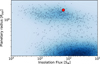 |
Fig. 1 Location of WASP-31b (red point) in radius versus insolation flux diagram of known exoplanets (small black points), zoomed-in on the hot-Jupiter region. Extracted from NASA Exoplanet archive on 24 March, 2025. |
2 Observations
We observed a total of three nights with ESPRESSO (as part of the GTO Working Group 2 (WG2)). The summary of the nights, including their respective program IDs, is provided in Table 2, with a full observation log per spectrum shown in Figure A.1.
The first and third nights are of comparable quality, with similar observing conditions and setup. The second night was stopped mid-transit due to degraded weather conditions, leaving only a few in-transit exposures to provide information about the planet. All three nights were observed using the Unit Telescope 1 (UT1) and STAR+SKY fiber reference mode (fiber B on sky background). We used the data-reduction software (DRS) to reduce the data (ESPRESSO DRS 3.0.0).
The ESPRESSO radial-velocity (RV) curve (Figure 2) shows a clear Rossiter-McLaughlin effect, suggesting an aligned planet, as previously observed by Brown et al. (2012). However, due to the larger mirror size, the precision of ESPRESSO RVs is much higher compared to those of the previous observation of HARPS. While two nights’ of HARPS observations exist (the aforementioned data used by Brown et al. (2012) and a single transit in the HEARTS survey; prog. ID: 097.C-1025(C), PI: D. Ehrenreich), we did not use the HARPS data due to the lower S/N. In particular, the transmission spectra from HARPS are much more dominated by red noise due to the lower S/N, while the RM analysis does not provide further information.
Simultaneously to the ESPRESSO observations, we followed the target using the ECAM (Lendl et al. 2012) at the 1.2 m Swiss telescope. While photometry analysis was not the focus of our study, these data were used to refine the ephemeris and to detect potential stellar activity during the transit.
System parameters
Observation log table.
3 Methodology
In Sect. 3.1, we discuss the simultaneous photometry analysis obtained with ECAM. Our methodology for transmission spectroscopy follows Steiner et al. (2023), which is based on the same pipeline1. However, multiple improvements to the pipeline have been made since then, which we describe below. Furthermore, RM effect analysis has been implemented in this pipeline recently (following Cegla et al. (2016); Bourrier et al. (2021)), so we describe the methodology used in this paper in Sect. 3.2.
3.1 Simultaneous photometry analysis
Simultaneously with the ESPRESSO observations, we obtained transit light curves using the ECAM (Lendl et al. 2012) at the ESO La Silla 1.2 m Swiss Telescope. These data were used in two ways during the analysis. First, each of the transit light curves was visually checked for potential stellar spots. Second, using the ECAM light curves combined with TESS, we attempted to refine the system parameters using CONAN (Lendl et al. 2017). Our results for stellar, planetary, and ephemeris parameters (Table 1, second column) are in good agreement with previous observations (third column). Because our analysis does not include the RV data, we do not obtain the mass of the planet, which is important for velocity calculation when shifting rest frames. Our ephemeris parameters are compatible with Kokori et al. (2023). However, our work is incompatible with previous observations by Patel & Espinoza (2022). We discuss the ephemeris choice used for our analysis in more detail in Appendix B.
Thus, in our analysis, we used the stellar and planetary parameters provided in the third column of Table 1, particularly those by Anderson et al. (2011), which we combine with the ephemeris and RM anomaly values from our analysis. The resulting light curves and the best-fit model are shown in Figure 3.
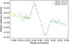 |
Fig. 2 Radial-velocity observations of ESPRESSO data. The Rossiter-McLaughlin anomaly is visible, showing the typical signature of an aligned planet as previously deduced by Brown et al. (2012) using a single HARPS transit. Nights are color-coded separately in blue (night #1), orange (#2), and green (#3). |
3.2 Analysis of RM anomaly
To analyze the RM anomaly, we used the “revolutions” method (Bourrier et al. 2021), which further builds on the “reloaded” method by Cegla et al. (2016). The RM anomaly analysis we performed was done on the CCF_SKYSUB_A products. These products are the output of the cross-correlation of the stellar template with the observed spectrum corrected for sky background and, as such, consist of an array of velocities, flux, and uncertainties. These CCFs are roughly Gaussian in shape, which, when fit, provides the observed RV of a given spectrum. We only used the combined CCF of all spectral orders in our analysis.
Before the analysis, we defined the light-curve model using batman (Kreidberg 2015) with the parameters as reported in Table 1. For limb-darkening coefficients, we used LDCU2 (Deline et al. 2022) to calculate the quadratic law coefficients, which were then passed to batman. We simulated a transit light curve for BJD timestamps of all CCFs.
The first step in our analysis is to normalize the CCFs to 1. To accomplish this, we fit a Gaussian profile with a constant term: G(A, σ, v0) + C, where G is the Gaussian profile with amplitude (contrast) A, standard deviation σ and mean value of v0, while the term C is our continuum trend (assumed constant). By dividing by C, we normalized each CCF to 1.
We furthermore scaled each CCF to their respective light-curve fluxes (Δ(t) = 1 − δ(t)), as calculated before by batman. Here, Δ(t) is the normalized light-curve flux, and δ is the transit depth due to the planet at a given time (0 when the planet is not transiting). Thus, the final normalized CCF is given by
![Mathematical equation: $\[\mathrm{CCF}_i(t)=\frac{\mathrm{CCF}_{\mathrm{i}; \text { raw }}}{C_i} \Delta_i(t).\]$](/articles/aa/full_html/2026/04/aa55811-25/aa55811-25-eq15.png) (1)
(1)
As the CCFs are in the barycenter of the Solar System, we needed to shift by the systemic velocity and the stellar velocity induced by the planet to the stellar rest frame. We calculated the systemic velocity for each night by fitting a master-out CCF3, following Bourrier et al. (2021), as there might be offsets between nights. All CCFs are first shifted by the stellar velocity, assuming a circular orbit given parameters from Table 1. Then we calculated the master-out CCF (average out-of-transit CCF), which we fit with a Gaussian profile. The mean value of this profile provides the systemic velocity of each night, which we used to shift our CCFs accordingly.
Then, we took the original set of CCFs in the solar barycentric rest frame, where we shifted by the previously calculated systemic velocity and stellar velocity induced by the planet. There, we calculated the master-out CCF (MCCF; out). We then subtracted each CCF from the calculated master-out to obtain the residual CCF (CCFres) and the intrinsic CCF (CCFintr), which are scaled by transit depth. As CCFintr depends on δi, we did not calculate CCFintr for out-of-transit CCFs.
![Mathematical equation: $\[\mathrm{CCF}_{\mathrm{i}, \text {res}}=\left(M_{\mathrm{CCF}; \text {out}}-\mathrm{CCF}_i(t)\right)\]$](/articles/aa/full_html/2026/04/aa55811-25/aa55811-25-eq16.png) (2)
(2)
![Mathematical equation: $\[\mathrm{CCF}_{\mathrm{i}, \text {intr}, ~\text {in}}=\frac{\left(M_{\mathrm{CCF}; \text {out}}-\mathrm{CCF}_i(t)\right)}{\delta_i(t)}\]$](/articles/aa/full_html/2026/04/aa55811-25/aa55811-25-eq17.png) (3)
(3)
To inspect the quality of each intrinsic in-transit CCF, we followed Bourrier et al. (2021) with MCMC fitting of a Gaussian profile to the CCF. We used the PYMC package. We used non-informative priors, limited only by the range of the CCF output, which is possible to modify in the DRS. We used the No U-Turn Sampler (NUTS) in the MCMC, with 15 000 burning steps4 and 15 000 drawing steps (meaning the first 50% of steps are thrown away). We used 30 chains, which were run on each individual exposure. The final posterior plots are depicted in Figure C.1.
A visual inspection of the posterior plots (Figure C.1) showed several poorly defined exposures, particularly the first and last exposures in the transit sequence. We removed these from the analysis. More information on this can be found in Appendix C.1. Furthermore, during the first night, an anomaly was found in the contrast shape of the raw CCFi. This is likely connected to the higher asymmetry of the Gaussian profile during the first night, as opposed to the second and third nights, as the residuals show a clear systematic trend as well. We further discuss the contrast anomaly in Appendix C.2.
After the removal of ill-defined CCFi, intr, we proceeded with the global fitting of all in-transit CCFi, intr. We fit for the contrast, FWHM, veq sin(i), and λ. We tested multiple-order polynomials of contrast and FWHM trends as a function of limb-angle μ, following Bourrier et al. (2021) to fit the CCFi, intr. The tested models include a constant profile for all nights, night-specific constant profiles, a night-specific linear model, and quadratic models. Finally, as the second night holds only a few exposures, we also ran the linear and quadratic model assuming a zeroth order on the second night, specifically, to avoid overfitting. By comparing the BIC, we found the constant profile to be the preferred model. Therefore, we assumed the non-varying shape of the stellar CCF within the data, effectively neglecting the CLV effect, as based on our tests they can be neglected within the noise level. Thus, our final priors for the “revolutions” fit were:
![Mathematical equation: $\[\begin{aligned}& \text { contrast } \sim \mathcal{U}(0,1), \\& \text { FWHM } \sim \mathcal{U}(0,15) ~\mathrm{km} \mathrm{~s}^{-1}, \\& v_{\text {eq }} \sin \left(i_{\star}\right) \sim \mathcal{U}(0,10) ~\mathrm{km} \mathrm{~s}^{-1}, \\& \lambda \sim \mathcal{U}(-180,180) \text { deg, }\end{aligned}\]$](/articles/aa/full_html/2026/04/aa55811-25/aa55811-25-eq18.png) (4)
(4)
where veq sin(i⋆) is the projected equatorial rotation velocity of the star and λ is the projected spin-orbit angle. We again used non-informative priors on the contrast of the CCFs. We used an FWHM prior that is fully encompassing the FWHM measurement on the MCCF; out (12.5 km s−1). As the local stellar velocity depends on both veq sin(i⋆) and λ, we used these as our jump parameters. The priors for these are again non-informative, although we could have used values provided by Brown et al. (2017). We did not use those priors due to the different methodology used to obtain these values, making our observations fully independent of each other. For veq sin(i⋆), we used a prior restricted only by the shape of the MCCF; out. For λ, we used a uniform distribution across the full range of possible values. We assumed solid-body rotation. We used 30 chains for this MCMC analysis, with 15 000 burning and drawing steps.
The resulting intrinsic CCFs and the residuals of subtracting the best-fit model obtained by the MCMC analysis from the intrinsic CCFs are shown in Figure 4. For the second and third night, we see a good fit to the data, but the first night shows a systematic difference. This is likely due to the stellar lines being asymmetric during the first night. This could, for example, be due to a high spot coverage; however, a visual examination of the photometry (Figure 3) did not confirm this. We note that our method might not be sensitive enough during the ingress for spot detection.
The resulting corner plot is provided in Figure 5. To obtain the resulting values for λ and veq sin(i⋆), we used the median values of the posteriors. We used the highest density intervals (HDI) of 68.3% to obtain the 1σ values of each parameter. The results are summarized in Table 3.
Finally, we looked at the available TESS data to see whether the rotation period of the star could be constrained with a Lomb–Scargle periodogram analysis. Unfortunately, such attempts proved unsuccessful. Thus, the full 3D obliquity ψ is left unknown. We note, however, that systems with λ ≈ 0° are rarely truly aligned (Attia et al. 2023).
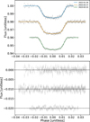 |
Fig. 3 Observed simultaneous photometric light curves (top panels) from ECAM for the three ESPRESSO nights. The best-fit models from CONAN for each night are color-coded separately in blue (night #1), orange (#2), and green (#3). The residuals for each night are shown in the bottom panel with an offset. The horizontal line is the continuum of 0. |
Results of RM analysis.
3.3 Transmission-spectroscopy extraction
The main change in our approach for extracting transmission spectroscopy is our use of the S1D_SKYSUB products, that is, the stitched echelle spectrum that is subtracted by the fiber B spectrum considering the differing fiber throughput. This means that telluric emission features, such as those of sodium, should already be corrected, and no further correction is necessary. We confirmed this by calculating the average fiber B spectrum per night and visually checking the prominent emission lines against the average fiber A spectrum per night (Figure 6).
The first step, as is common in this type of study (e.g., Allart et al. 2017; Seidel et al. 2020; Mounzer et al. 2022), is telluric line correction. We used molecfit (Smette et al. 2015; Kausch et al. 2015), which allows correction for absorption lines due to the Earth’s atmosphere in each exposure. To do so, molecfit considers the weather observations and runs a line-by-line radiative-transfer code to calculate a telluric transmission spectrum, such that it reproduces the observed spectra. We refer the reader to the above-mentioned references for more details about the procedure.
As an output, molecfit provides the user with the telluri-ccorrected spectrum and telluric profile used to correct each spectrum. As the telluric profile does not have an uncertainty, at wavelengths where the atmosphere is almost opaque, the corrected spectra produce features that are not well represented by their uncertainties. To remove them, we identified and replaced pixels with NaN values where the telluric profile was below 50%, indicating that less than half of the light is successfully transmitted through the Earth’s atmosphere. This procedure is relevant for the CCF study and lines falling in the telluric-contaminated regions (e.g., potassium). The effects of telluric correction by molecfit and sky-subtraction done by the DRS are shown in Figures 6 and 7.
After telluric correction, we interpolated the dataset on a common wavelength grid using a cubic spline interpolation. The data were then normalized with a rolling quantile of 85% and a window of 7500 pixels. We used a higher quantile than the standard median to more closely represent a stellar spectrum – the spectrum’s absorption features (stellar lines) are far more common than emission (mostly cosmic rays), meaning a median will represent the continuum less accurately. We note, however, that the choice of a normalization function is generally irrelevant as long as the method is not variable in time (since we eventually divided spectra by the master-out, the normalization function negates itself). Likewise, we also performed the analysis with a rolling median window to ensure this does not affect the results. The window of 7500 pixels was chosen empirically, such that the spectrum is mostly flat aside from the noisy blue edge of the detector.
The next step was to shift the telluric-corrected spectra from the solar barycenter rest frame to that of the host star, which was done by considering the systemic velocity and stellar velocity induced by the planet (note that the S1D_SKYSUB format of the used ESPRESSO DRS is in the solar barycenter, not the Earth’s rest frame). There, we calculated the master-out (average out of transit spectrum), again for each night separately, using an unweighted average. We divided the dataset by their respective master-out spectra to remove the stellar contribution to the spectra.
The spectra are inherently contaminated by the wiggles coming from the Coudé train (Allart et al. 2020; Tabernero et al. 2021) optical component in the optical path. These wiggles are currently difficult to correct, and multiple methods have been used to remove them (e.g., local sinusoidal fit (Seidel et al. 2022), cubic-spline fit (Damasceno et al. 2024), correction on the CCD image before spectrum extraction (Sedaghati et al. 2021), or analytical models (Bourrier et al. 2024)). In this work, we used a similar approach to Damasceno et al. (2024). We took a binned spectrum (a factor of 200 pixels), which we fit with cubic splines. We then divided the spectra by the cubic-spline fit to remove the wiggle contamination.
We then shifted the spectra to the planet’s rest frame by assuming the stellar (with a negative sign) and planetary velocity. There, we first focused our analysis on the combined transmission spectrum (average in-transit spectrum), using an unweighted average. Immediately, a strong POLD contamination is visible, as shown in Figure 8. This feature is dominant for most species that are also present in the star. The only exceptions to the lines we probed are lithium (Li), which does not have strong stellar absorption, and the first line of the hydrogen Balmer series (H α), which is extremely broad in the stellar spectrum, muting and broadening the effect on the final transmission spectrum.
We did not detect any species in the transmission spectrum. Instead, we estimated detection limits for the probed lines. We first adjusted the transmission spectrum by ![Mathematical equation: $\[R=1-\frac{\mathrm{F}_{\text {in}}}{\mathrm{M}_{\text {out}}}\]$](/articles/aa/full_html/2026/04/aa55811-25/aa55811-25-eq21.png) , where
, where ![Mathematical equation: $\[\frac{\mathrm{F}_{\text {in}}}{\mathrm{M}_{\text {out}}}\]$](/articles/aa/full_html/2026/04/aa55811-25/aa55811-25-eq22.png) is the in-transit spectrum divided by the master-out. Then, we created a Gaussian line model for each of the probed lines, with its mean value set to the laboratory line position. The FWHM of the line is set to the instrumental response of ESPRESSO. Finally, amplitude is kept as the sole jump parameter A ~ 𝒰(−1, 1). For POLD-corrected data (Na I H α and K), we ran a MCMC analysis on the transmission spectrum in the 6 Å region centered on the line position. For POLD-uncorrected data, we moved the model mean value to 20 km/s or 1 Å. This was done in order to avoid fitting the POLD feature visible in the data, while maintaining the noise behavior in the continuum. The 1σ uncertainty was then extracted based on the 68.3% HDI.
is the in-transit spectrum divided by the master-out. Then, we created a Gaussian line model for each of the probed lines, with its mean value set to the laboratory line position. The FWHM of the line is set to the instrumental response of ESPRESSO. Finally, amplitude is kept as the sole jump parameter A ~ 𝒰(−1, 1). For POLD-corrected data (Na I H α and K), we ran a MCMC analysis on the transmission spectrum in the 6 Å region centered on the line position. For POLD-uncorrected data, we moved the model mean value to 20 km/s or 1 Å. This was done in order to avoid fitting the POLD feature visible in the data, while maintaining the noise behavior in the continuum. The 1σ uncertainty was then extracted based on the 68.3% HDI.
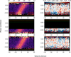 |
Fig. 4 Intrinsic CCF per night (left panels) and their respective residuals (right panels). The RM signature is well visible during the transit as a bright track. The dashed horizontal lines correspond to T14 contact points (orange) and T23 (green). The solid red lines (with black outlines) correspond to spectra that were excluded from the analysis. The dotted black lines correspond to the expected local stellar velocity using the best-fit model. The first night’s residuals show a systematic trend, likely due to line asymmetry. |
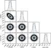 |
Fig. 5 Final posterior corner plot of e revolutions analysis of RM anomaly. All values are well-defined, with an anticorrelation between the contrast and FWHM of the line profile. The contours show 1σ, a region containing 50% of accepted steps and 2σ levels, as defined by the corner package. The solid lines correspond to the median value of the posterior distribution function, which is used as the measured value. |
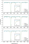 |
Fig. 6 Correction for fiber B and telluric lines in the region of the sodium doublet. Each panel shows a respective night, with the master of raw spectra from fiber A (uncorrected for fiber B and telluric lines) in orange. In green, we show the master of fiber A spectra corrected for fiber B and telluric lines. The respective average telluric profile and fiber-B emission are shown in blue and gray, respectively. Please note that fiber B is on an arbitrary scale due to normalization. The zoomed-in image of the inset focuses on the wavelength region of 5890–5891 Å. |
4 Transmission spectroscopy
After extracting the transmission spectrum, we checked for resolved line detections, following the list of lines detected by Borsa et al. (2021) in WASP-121 b. This list includes lines of Na, H, K, Li, Ca, Mn, and Mg and consists of the easiest lines (detectability-wise) to resolve in the spectra. However, most of these species are likely condensed in the atmosphere of WASP-31 b, owing to its lower temperature compared to WASP-121 b. We focused our endeavor on Na I and H α. Furthermore, we cross-correlated a forward model generated by petitRADTRANS (Mollière et al. 2019) to look for Fe. In Sect. 4.1, we discuss the transmission spectroscopy of the Na I and H α lines that can be resolved individually. The cross-correlation of iron is discussed in Sect. 4.3, and the cross-correlation of CrH is discussed in Sect. 4.4.
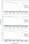 |
Fig. 7 Same as Figure 6, but in region of H α. No strong telluric features were detected in this region. |
4.1 Resolved line-transmission spectroscopy of sodium and hydrogen
The transmission spectra for Na I and H α are shown in Figure 8. The Na I doublet, as most other probed lines, is thoroughly contaminated by POLDs. For these lines, we typically see a negative core (as is the case for HD 209458 b (Casasayas-Barris et al. 2020, 2021)), with weaker positive wings. This makes the detection of the species difficult, as we require forward modeling for both atmosphere and POLD contamination simultaneously to securely distinguish between the signals. We modeled the POLD deformation with EvE (Bourrier & Lecavelier des Etangs 2013; Bourrier et al. 2015, 2016), as discussed in Section 4.2.
H α is much broader (and weaker) in the stellar spectrum, causing the POLD distortion to be more spread out and weaker. Furthermore, once combined, the POLDs in the spectral time series cancel each other out, decreasing the amplitude of the deformation. Nevertheless, a visible negative plateau is present, ranging over almost 1 Å (Figure 8). Within it, we see a weak and narrow signal, which is blueshifted roughly by 10km s−1. We discuss this further in Section 4.2.
4.2 Joint stellar and planet modeling with EvE
To account correctly for POLDs, we followed the methodology by Dethier & Bourrier (2023) using the EvE code. For the simulations, we used values of the system as provided in Table 1, with λ and v sin(i⋆) as measured by our analysis (Table 3). More details about EvE can be found in Bourrier & Lecavelier des Etangs (2013); Bourrier et al. (2016); Dethier & Bourrier (2023) and Steiner et al. (2023).
As no visible signal is detected for sodium, we first simulated a planet disk devoid of an atmosphere. This led to a model that matches the observed signal very well (orange line in top panel; Figure 8). Thus, within our uncertainties, we can fully explain the signal as POLD deformations in the transmission spectra. We show the resulting transmission spectrum and the models in Figure 8.
For the H α line, due to the hint of a weak signal (possibly due to atmosphere) (Figure 8), we opted for a two-step approach. First, we modeled the transit by simulating a planet disk without any atmosphere. This allows us to show the strength of the POLD effect, which, in this case, is much weaker than in the Na I case (orange line in bottom panel; Figure 8). The narrow blueshifted signature seen in the spectra is not explained by this simulation. The width of this feature is close to the instrumental response function (blue line in bottom panel; Figure 8), suggesting it might be an unresolved line. In the second step, we include a realistic atmosphere around the planet to simulate the transit with its atmosphere passing (green line in bottom panel; Figure 8). The simulation leads to a solution in which the atmospheric signature is much broader (albeit of similar strength) than the observed signal as shown in Figure 8.
Neither of these models fully explains the observation. In particular, neither can clearly explain the amplitude of the negative core of the POLD distortion. The “no-atmosphere” model (orange line in bottom panel; Figure 8) for H α underestimates the amplitude by a factor of ~10. This model does not reproduce the feature observed at 6562.5 Å, for which we attempted to use an atmosphere model in EvE. The modeled atmospheric signature (green line in bottom panel; Figure 8) is much wider than what we observed, and, as such, we attempted to match the width of the line by decreasing the input temperature in EvE. Lowering the equilibrium temperature to 750 K (half of the value reported by Anderson et al. (2011)) did not significantly affect the width of the modeled atmospheric line. The atmospheric density profile is computed with a hydrostatic profile. The temperature profile is isothermal. Day-to-night-side wind was applied as a bulk wind to the atmosphere. Rotation of the planet and the atmosphere were indeed taken into account, considering the planet tidally locked. Therefore, the included broadening of the line is due to the temperature and rotation of the atmosphere. We observe this feature on all nights (Appendix E). Given the instrumental response function, the observed feature, if real, might be an unresolved line, potentially an alias line with the Balmer alpha. Within the region of 6562–6563 Å, the potential candidates, except for H α, are V II (6562.4 Å), Li II (6562.61 Å), Th I (6562.647 Å), and Au I (6562.68 Å). The upper-limits of the non-detections of Na and H α are provided in the Table 4.
As other species (aside from Na I and H α) were outside the main scope of this paper, we did not simulate the POLD effect on the rest of the species (Appendix D). For Li, we do not see POLD deformation, as the spectral line does not appear in the stellar spectrum. For other lines, we see strong negative features, similar to the Na I POLD deformations.
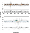 |
Fig. 8 Combined transmission spectrum and its residuals of WASP-31b in the region of sodium doublet (top panels), and Balmer alpha line (bottom panels) in the rest frame of the planet. We plot the full spectrum in gray; that binned by 15x is shown in black. In this notation, absorption goes above zero, and “emission” is below. The laboratory position of the respective lines is shown via dashed black lines. The no-atmosphere model from EvE is plotted as an orange line, and the compound model with the atmosphere is shown as a green line. The vertical dashed green lines correspond to the escape velocity of ≈33 km/s, centered on the feature at 6562.5Å. The instrumental response function of ESPRESSO is centered on this feature in blue. Residuals were calculated assuming the no-atmosphere model. |
Upper limits for Na I and H α with the corresponding height in planetary radii in parentheses.
4.3 Cross-correlation function of iron
The iron template model was generated using the system parameters, as reported by Table 1, assuming the Guillot T-P profile (Guillot et al. 2023) with pressures between [10−10; 102] bar. We assumed weighting by the pixel’s uncertainty, that is5:
![Mathematical equation: $\[w_i=\frac{1}{\sigma_i^2},\]$](/articles/aa/full_html/2026/04/aa55811-25/aa55811-25-eq23.png) (5)
(5)
where the CCF calculation follows Hoeijmakers et al. (2019) with a few modifications due to weighting and a non-normalized template.
![Mathematical equation: $\[\operatorname{CCF}(t, v)=\frac{\sum_i^N x_i(t) T_i(v) w_i(t)}{\sum_i^N T_i(v) w_i(t)},\]$](/articles/aa/full_html/2026/04/aa55811-25/aa55811-25-eq24.png) (6)
(6)
here, the i corresponds to each pixel of the spectrum, with its respective weight, wi. The template Ti(v) is the previously generated model from petitRADTRANS, and xi(t) is the spectrum at time t.
We show the resulting phase-resolved CCF in Figure 9, and the combined 1D CCF in Figure 10. We see a strong contamination from the POLD effect, with no atmospheric signature within. As shown in Figure 9, the planetary track is almost unresolvable from the Doppler shadow.
4.4 Cross-correlation function of chromium hydride
WASP-31b is the first exoplanet on which a chromium-hydride (CrH) detection has been noted, first tentatively using HST STIS/WFC (Braam et al. 2021), and later with high-resolution spectroscopy using GRACES and UVES (Flagg et al. 2023). While CrH only has negligible opacity throughout most of the optical bandpass, it does have some weak spectral lines redward of ~690 nm and its main molecular bands starting at ~765 nm. While this leaves only a small portion of the ESPRESSO detector (380–780 nm) overlapping with CrH lines, in light of the previous detections, we nevertheless opted to search for CrH absorption in the transmission time series of WASP-31b.
As the high-resolution detection of CrH by Flagg et al. (2023) was made from a data detrending method based on singular-value decomposition, we opted to use a similar approach, in contrast to the molecfit-based telluric correction used for our main analysis. For this, we processed the data using the principal-component-analysis (PCA) based detrending framework of Pelletier et al. (2021, 2023, 2024); Bazinet et al. (2024). In short, this algorithm processes each spectral order of each transit time series, wherein all spectra are corrected for bad pixels, aligned to a common continuum level, corrected for out-of-transit median spectra, and divided by a five-principal-component reconstruction of the data. The analysis procedure closely follows Pelletier et al. (2024), to which we refer the reader for more details. We also cross-correlated the CrH template following our main molecfit-based approach as described in Sects. 3.3 and 4.3, finding compatible results.
For the cross-correlation, we generated a fiducial solar composition (Asplund et al. 2009) chemical-equilibrium transmission template of WASP-31b using the SCARLET atmosphere modeling framework (Benneke & Seager 2012, 2013; Benneke 2015; Benneke et al. 2019) (by default, petitRADTRANS does not provide CrH line lists at high spectral resolution). The CrH cross-sections used in the model were computed from the line list of Burrows et al. (2002) using HELIOS-K (Grimm & Heng 2015; Grimm et al. 2021). Chemical-equilibrium abundance profiles were calculated using FastChem (Stock et al. 2018, 2022) assuming the thermal structure of the atmosphere of WASP-31b to be isothermal at an equilibrium temperature of 1393 K (Braam et al. 2021) and having a gray cloud deck at 100 mbar. CrH has the advantage that, unlike Na and other neutral metals, it is not expected to be present in the stellar photosphere and hence should not be contaminated by the POLD effect.
We then cross-correlated the CrH transmission template, once with the detrended data, and once with the detrended data after the generated WASP-31b transmission template had been injected in the transit time series (before detrending) on top of the real signal. This latter scenario of injecting and recovering a realistic model of the atmosphere of WASP-31b in the data serves as a sensitivity test of how strongly our observations should detect an underlying real signal. While we do not find any evidence of CrH absorption in the ESPRESSO transit data, based on the injection-recovery test, we also likely would not have been sensitive to a real signal (Figure 11). We therefore cannot confirm (or refute) the CrH detection on WASP-31b, largely owing to the coverage of ESPRESSO being limited to wavelengths blueward of 780 nm. In particular, we note that the CrH detection made by Flagg et al. (2023) used the 860–895 nm wavelength range not covered by our data.
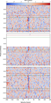 |
Fig. 9 Phase-resolved cross-correlation of iron template with the dataset of WASP-31b, in the rest frame of the star. Each panel corresponds to a separate night (top panel for first night, middle for second, and bottom for third night). The contact points T1–T4 are plotted as red horizontal dashed lines, with contact points T2–T3 shown as horizontal dashed green lines. The planetary track is shown as a dashed line blue for the out-of-transit section. Absorption features are shown in red (positive) and negative features in blue. |
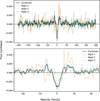 |
Fig. 10 Cross-correlation of iron template with the combined and night-specific transmission spectroscopy in the rest frame of the planet. The combined CCF of all nights is shown in black, with the nights shown separately in blue (night 1), orange (night 2), and green (night 3). The top panel shows the full velocity range over which the CCF was calculated. The bottom panel shows a zoomed-in view of −50,50 km s−1. Absorption is positive with respect to the continuum. |
5 Discussion
We confirm the measurement of the sky-projected spin-orbit angle of WASP-31b, as shown by Brown et al. (2012). Our precision suggests almost perfect projected alignment; however, as shown in Attia et al. (2023), the true spin-orbit angle is likely to be underestimated. An analysis of the photometry did not lead to stellar rotation-period measurement needed for the measurement of i⋆ and the derivation of the 3D spin-orbit.
The non-detection of the resolved lines Na, K, Mg, Ca, and Mn is expected, as the contamination by the POLD effect hides any potential signal. We modeled the POLDs with a cutting-edge model to assess that the low-significance feature observed at H α does not originate from POLDs. Li is an exception to the list of lines polluted by POLDs, as the host star does not exhibit significant absorption of Li, which removes any contamination by the POLD effect.
We illustrate the difficulty of achieving atmospheric detections due to POLD effects in Figure 12, showing the (non-)detections of sodium, depending on alignment. As shown, misalignment almost ensures an atmosphere’s detectability, as the POLD contamination can be distinguished from the planetary track. The majority of the planets with sodium detection claims are for hot and ultra-hot Jupiters, for which a significant amount of data exists, including high-resolution spectrographs. We note, however, that there is likely observational bias due to a low number of non-detection publications. In WASP-31 b, the combination of system parameters leads to the orbital track being undistinguishable from the Doppler shadow, as illustrated in Figure 9.
The case of H α is quite unique, as it is the only species present in the stellar spectrum not visibly contaminated by the POLD effect. This is likely due to the fact that the POLDs effect scales with the stellar line gradient and is muted for very broad lines such as H α. Indeed, modeling of the POLDs effects shows a small amplitude deformation. Inside the transmission spectrum, we observe a low S/N feature of unknown origin, either due to possible detection of H α, or due to noise in the spectra. As the significance of the feature is below 3σ, we do not claim any detection from the present data.
In the CCF regime, we looked for iron as the main species within the ESPRESSO wavelength range. However, Fe is severely contaminated by POLDs, disallowing any form of detection limit extraction. On the other hand, the non-detection of iron is indicative of a cloud deck, which is expected for these kinds of systems.
Finally, we attempted to search for CrH in our data, which had been suggested by Braam et al. (2021) and then confirmed by Flagg et al. (2023). For methodology reasons, we used a different pipeline in order to align our work with the methodology followed by Flagg et al. (2023). However, as can be seen from Figure 11, we are unable to detect expected signal from the injection-recovery test, which is likely due to the low sensitivity of CrH in the wavelength range of ESPRESSO. Thus, we make no claim on the presence of CrH in the atmosphere of WASP-31 b.
These results highlight the difficulty of making high-resolution observations for aligned exoplanets, which could suggest that a better observing strategy for high-resolution spectroscopy might be needed, particularly in light of the future ELT/ANDES observations of terrestrial planets. This could motivate a two-step approach of using high-resolution spectrographs at smaller telescopes to observe the projected spin-orbit angle, applying a filter to the target selection based on the overlap of the planetary track with the core POLD contamination. Alternatively, the use of models simulating both the planetary disk and the atmosphere, as EvE does, could be used to detect and characterize signatures when the planetary tracks are unresolved from the Doppler shadow.
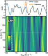 |
Fig. 11 Chromium-hydride (CrH) cross-correlation search and sensitivity check. The bottom panel shows the phase-folded Kp-Vsys signal-to-noise map of the ESPRESSO WASP-31b transit data cross-correlated with a CrH model template. The dashed lines denote the expected values of (Vsys = −0.1 km s−1, and Kp = 148.0 km s−1, Gaia Collaboration 2023; Flagg et al. 2023). The top panel shows a one-dimensional slice at the expected Kp (along the horizontal dashed white line) for both the data alone (blue) and the data with an injected model (orange). The difference between the blue and orange lines is a measure of the data sensitivity to an underlying signal. In this case, these data only have limited sensitivity to CrH, which has its strongest opacity band heads redward of the ESPRESSO wavelength coverage. Although no clear CrH signal is observed in the data here, we cannot conclusively confirm or rule out its presence in the atmosphere of WASP-31b due to limited sensitivity. |
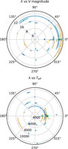 |
Fig. 12 Detections (blue) and non-detections (orange) of Na I doublet lines using high-resolution spectrographs based on projected spin-orbit angles (λ) of the system. The green point is the position of WASP-31 b found using our observed values for λ. The top panel shows the (non-)detections with respect to V magnitude. The bottom panel shows the (non-)detections with respect to Teff of the host star. Data were extracted on 7 March, 2025. Although sodium detections exist spanning vastly different orbital alignments, non-detections show a clear preference for aligned systems (1st and 3rd quadrants); however, given the small number of non-detection publications and the higher chance of close-in giants being aligned, we cannot distinguish them from observational bias. |
6 Conclusions
In this work, we analyzed the ESPRESSO dataset of WASP-31b, an inflated hot Jupiter. We first analyzed the RM signature using the revolutions method (Bourrier et al. 2021), which allowed us to constrain the projected obliquity to λ = ![Mathematical equation: $\[-0.09_{-0.32}^{+0.31}\]$](/articles/aa/full_html/2026/04/aa55811-25/aa55811-25-eq25.png) deg and projected stellar rotation to v sin(i⋆) =
deg and projected stellar rotation to v sin(i⋆) = ![Mathematical equation: $\[7.42_{-0.11}^{+0.11}\]$](/articles/aa/full_html/2026/04/aa55811-25/aa55811-25-eq26.png) km/s, increasing the precision by factors of ten and seven, respectively, with regard to previous works (Brown et al. 2012).
km/s, increasing the precision by factors of ten and seven, respectively, with regard to previous works (Brown et al. 2012).
Our analysis shows significant contamination of the transmission spectra by the POLD effect, which effectively disallows the analysis of lines that are present in the star. The only exceptions are the broadened H α, where the POLD signature is much weaker due to the stellar line broadness, and Li, which does not show a stellar line. The POLD contamination is also visible in the CCF regime, where we looked for iron.
Finally, as WASP-31b is the first planet with CrH detection (Braam et al. 2021; Flagg et al. 2023), we tried to perform a CCF with this species as well. We do not detect any CrH; however, using an injection-recovery test, we show that we are unable to extract reliable detection with this dataset, in particular due to the wavelength range of ESPRESSO not overlapping with strong CrH lines.
This paper highlights the need to distinguish the planetary track from the core of the POLDs effect, which is one of the core issues in transmission spectroscopy at the advent of the ELT observations.
Acknowledgements
This project has received funding from the European Research Council (ERC) under the European Union’s Horizon 2020 research and innovation programme (project Four Aces; grant agreement No. 724427). MS and VB’s work has been carried out in the frame of the National Centre for Competence in Research PlanetS supported by the Swiss National Science Foundation (SNSF). MS and VB acknowledge funding from the European Research Council (ERC) under the European Union’s Horizon 2020 research and innovation programme (project Spice Dune; grant agreement No 947634). It has also been carried out in the frame of the National Centre for Competence in Research PlanetS supported by the Swiss National Science Foundation (SNSF). MS, DE and VV acknowledges financial support from the SNSF for project 200021_200726. Co-funded by the European Union (ERC, FIERCE, 101052347). Views and opinions expressed are however those of the author(s) only and do not necessarily reflect those of the European Union or the European Research Council. Neither the European Union nor the granting authority can be held responsible for them. This work was supported by FCT – Fundação para a Ciência e a Tecnologia through national funds by these grants: UIDB/04434/2020 DOI: 10.54499/UIDB/04434/2020, UIDP/04434/2020 DOI: 10.54499/UIDP/04434/2020. R.A. acknowledges the Swiss National Science Foundation (SNSF) support under the Post-Doc Mobility grant P500PT_222212 and the support of the Institut Trottier de Recherche sur les Exoplanètes (iREx). This work has been carried out within the framework of the National Centre of Competence in Research PlanetS supported by the Swiss National Science Foundation. The authors acknowledge the financial support of the SNSF. The INAF authors acknowledge financial support of the Italian Ministry of Education, University, and Research with PRIN 201278X4FL and the “Progetti Premiali” funding scheme. JIGH, ASM, CAP, and RR acknowledge financial support from the Spanish Ministry of Science, Innovation and Universities (MICIU) projects PID2020-117493GB-I00 and PID2023-149982NB-I00. This work was financed by Portuguese funds through FCT (Fundação para a Ciência e a Tecnologia) in the framework of the project 2022.04048.PTDC (Phi in the Sky, DOI 10.54499/2022.04048.PTDC). CJM also acknowledges FCT and POCH/FSE (EC) support through Investigador FCT Contract 2021.01214.CEECIND/CP1658/CT0001 (DOI 10.54499/2021.01214.CEECIND/CP1658/CT0001). We acknowledge financial support from the Agencia Estatal de Investigación of the Ministerio de Ciencia e Innovación MCIN/AEI/10.13039/501100011033 and the ERDF “A way of making Europe” through project PID2021-125627OB-C32, and from the Centre of Excellence “Severo Ochoa” award to the Instituto de Astrofísica de Canarias. A.P. acknowledges grants from the Spanish program Unidad de Excelencia María de Maeztu CEX2020-001058-M, 2021-SGR-1526 (Generalitat de Catalunya), and support from the Generalitat de Catalunya/CERCA. This work has been carried out within the framework of the NCCR PlanetS supported by the Swiss National Science Foundation under grants 51NF40_182901 and 51NF40_205606. FPE and CLO would like to acknowledge the Swiss National Science Foundation (SNSF) for supporting research with ESPRESSO through the SNSF grants nos. 140649, 152721, 166227, 184618 and 215190. The ESPRESSO Instrument Project was partially funded through SNSF’s FLARE Programme for large infrastructures. Apart from the already mentioned software, this project used Python (version 3.10.12) and its respective implemented libraries. Furthermore, these external packages were also utilized: astropy (Astropy Collaboration 2022), specutils, numpy, scipy, matplotlib and pandas, mpire, pyvo, seaborn and bokeh.
References
- Allart, R., Lovis, C., Pino, L., et al. 2017, A&A, 606, A144 [NASA ADS] [CrossRef] [EDP Sciences] [Google Scholar]
- Allart, R., Pino, L., Lovis, C., et al. 2020, A&A, 644, A155 [NASA ADS] [CrossRef] [EDP Sciences] [Google Scholar]
- Anderson, D. R., Collier Cameron, A., Hellier, C., et al. 2011, A&A, 531, A60 [NASA ADS] [CrossRef] [EDP Sciences] [Google Scholar]
- Asplund, M., Grevesse, N., Sauval, A. J., & Scott, P. 2009, Annu. Rev. A&A, 47, 481 [Google Scholar]
- Astropy Collaboration (Price-Whelan, A. M., et al.) 2022, ApJ, 935, 167 [NASA ADS] [CrossRef] [Google Scholar]
- Attia, O., Bourrier, V., Delisle, J. B., & Eggenberger, P. 2023, A&A, 674, A120 [NASA ADS] [CrossRef] [EDP Sciences] [Google Scholar]
- Azevedo Silva, T., Demangeon, O. D. S., Santos, N. C., et al. 2022, A&A, 666, L10 [NASA ADS] [CrossRef] [EDP Sciences] [Google Scholar]
- Bazinet, L., Pelletier, S., Benneke, B., Salinas, R., & Mace, G. N. 2024, AJ, 167, 206 [NASA ADS] [CrossRef] [Google Scholar]
- Benneke, B. 2015, arXiv e-prints [arXiv:1504.07655] [Google Scholar]
- Benneke, B., & Seager, S. 2012, ApJ, 753, 100 [NASA ADS] [CrossRef] [Google Scholar]
- Benneke, B., & Seager, S. 2013, ApJ, 778, 153 [Google Scholar]
- Benneke, B., Knutson, H. A., Lothringer, J., et al. 2019, Nat. Astron., 3, 813 [Google Scholar]
- Bonomo, A. S., Desidera, S., Benatti, S., et al. 2017, A&A, 602, A107 [NASA ADS] [CrossRef] [EDP Sciences] [Google Scholar]
- Borsa, F., Allart, R., Casasayas-Barris, N., et al. 2021, A&A, 645, A24 [EDP Sciences] [Google Scholar]
- Bourrier, V., & Lecavelier des Etangs, A. 2013, A&A, 557, A124 [NASA ADS] [CrossRef] [EDP Sciences] [Google Scholar]
- Bourrier, V., Ehrenreich, D., & Lecavelier des Etangs, A. 2015, A&A, 582, A65 [NASA ADS] [CrossRef] [EDP Sciences] [Google Scholar]
- Bourrier, V., Lecavelier des Etangs, A., Ehrenreich, D., Tanaka, Y. A., & Vidotto, A. A. 2016, A&A, 591, A121 [NASA ADS] [CrossRef] [EDP Sciences] [Google Scholar]
- Bourrier, V., Lovis, C., Cretignier, M., et al. 2021, A&A, 654, A152 [NASA ADS] [CrossRef] [EDP Sciences] [Google Scholar]
- Bourrier, V., Zapatero Osorio, M. R., Allart, R., et al. 2022, A&A, 663, A160 [NASA ADS] [CrossRef] [EDP Sciences] [Google Scholar]
- Bourrier, V., Delisle, J. B., Lovis, C., et al. 2024, A&A, 691, A113 [NASA ADS] [CrossRef] [EDP Sciences] [Google Scholar]
- Braam, M., van der Tak, F. F. S., Chubb, K. L., & Min, M. 2021, A&A, 646, A17 [NASA ADS] [CrossRef] [EDP Sciences] [Google Scholar]
- Brown, T. M. 2001, ApJ, 553, 1006 [NASA ADS] [CrossRef] [Google Scholar]
- Brown, D. J. A., Cameron, A. C., Anderson, D. R., et al. 2012, MNRAS, 423, 1503 [NASA ADS] [CrossRef] [Google Scholar]
- Brown, D. J. A., Triaud, A. H. M. J., Doyle, A. P., et al. 2017, MNRAS, 464, 810 [Google Scholar]
- Burrows, A., Ram, R. S., Bernath, P., Sharp, C. M., & Milsom, J. A. 2002, ApJ, 577, 986 [NASA ADS] [CrossRef] [Google Scholar]
- Carteret, Y., Bourrier, V., & Dethier, W. 2024, A&A, 683, A63 [NASA ADS] [CrossRef] [EDP Sciences] [Google Scholar]
- Casasayas-Barris, N., Palle, E., Nowak, G., et al. 2017, A&A, 608, A135 [NASA ADS] [CrossRef] [EDP Sciences] [Google Scholar]
- Casasayas-Barris, N., Pallé, E., Yan, F., et al. 2020, A&A, 635, A206 [NASA ADS] [CrossRef] [EDP Sciences] [Google Scholar]
- Casasayas-Barris, N., Palle, E., Stangret, M., et al. 2021, A&A, 647, A26 [NASA ADS] [CrossRef] [EDP Sciences] [Google Scholar]
- Cegla, H. M., Lovis, C., Bourrier, V., et al. 2016, A&A, 588, A127 [NASA ADS] [CrossRef] [EDP Sciences] [Google Scholar]
- Charbonneau, D., Brown, T. M., Noyes, R. W., & Gilliland, R. L. 2002, ApJ, 568, 377 [Google Scholar]
- Chen, G., Casasayas-Barris, N., Pallé, E., et al. 2020, A&A, 635, A171 [NASA ADS] [CrossRef] [EDP Sciences] [Google Scholar]
- Cristo, E., Santos, N. C., Demangeon, O., et al. 2022, A&A, 660, A52 [NASA ADS] [CrossRef] [EDP Sciences] [Google Scholar]
- Damasceno, Y. C., Seidel, J. V., Prinoth, B., et al. 2024, A&A, 689, A54 [NASA ADS] [CrossRef] [EDP Sciences] [Google Scholar]
- Deline, A., Hooton, M. J., Lendl, M., et al. 2022, A&A, 659, A74 [NASA ADS] [CrossRef] [EDP Sciences] [Google Scholar]
- Dethier, W., & Bourrier, V. 2023, A&A, 674, A86 [NASA ADS] [CrossRef] [EDP Sciences] [Google Scholar]
- Dethier, W., & Tessore, B. 2024, A&A, 688, L30 [NASA ADS] [CrossRef] [EDP Sciences] [Google Scholar]
- Ehrenreich, D., Lovis, C., Allart, R., et al. 2020, Nature, 580, 597 [Google Scholar]
- Flagg, L., Turner, J. D., Deibert, E., et al. 2023, ApJ, 953, L19 [NASA ADS] [CrossRef] [Google Scholar]
- Gaia Collaboration (Vallenari, A., et al.) 2023, A&A, 674, A1 [NASA ADS] [CrossRef] [EDP Sciences] [Google Scholar]
- Gibson, N. P., Nikolov, N., Sing, D. K., et al. 2017, MNRAS, 467, 4591 [NASA ADS] [CrossRef] [Google Scholar]
- Gibson, N. P., de Mooij, E. J. W., Evans, T. M., et al. 2019, MNRAS, 482, 606 [CrossRef] [Google Scholar]
- Grimm, S. L., & Heng, K. 2015, ApJ, 808, 182 [NASA ADS] [CrossRef] [Google Scholar]
- Grimm, S. L., Malik, M., Kitzmann, D., et al. 2021, ApJS, 253, 30 [NASA ADS] [CrossRef] [Google Scholar]
- Guillot, T., Fletcher, L. N., Helled, R., et al. 2023, arXiv e-prints [arXiv:2205.04100] [Google Scholar]
- Hoeijmakers, H. J., Ehrenreich, D., Kitzmann, D., et al. 2019, A&A, 627, A165 [NASA ADS] [CrossRef] [EDP Sciences] [Google Scholar]
- Jiang, C., Chen, G., Murgas, F., et al. 2024, A&A, 682, A73 [NASA ADS] [CrossRef] [EDP Sciences] [Google Scholar]
- Kausch, W., Noll, S., Smette, A., et al. 2015, A&A, 576, A78 [NASA ADS] [CrossRef] [EDP Sciences] [Google Scholar]
- Kokori, A., Tsiaras, A., Edwards, B., et al. 2023, ApJS, 265, 4 [NASA ADS] [CrossRef] [Google Scholar]
- Kreidberg, L. 2015, PASP, 127, 1161 [Google Scholar]
- Lendl, M., Anderson, D. R., Collier-Cameron, A., et al. 2012, A&A, 544, A72 [NASA ADS] [CrossRef] [EDP Sciences] [Google Scholar]
- Lendl, M., Cubillos, P. E., Hagelberg, J., et al. 2017, A&A, 606, A18 [NASA ADS] [CrossRef] [EDP Sciences] [Google Scholar]
- McLaughlin, D. B. 1924, ApJ, 60, 22 [Google Scholar]
- Mollière, P., Wardenier, J. P., van Boekel, R., et al. 2019, A&A, 627, A67 [Google Scholar]
- Morello, G., Casasayas-Barris, N., Orell-Miquel, J., et al. 2022, A&A, 657, A97 [NASA ADS] [CrossRef] [EDP Sciences] [Google Scholar]
- Mounzer, D., Lovis, C., Seidel, J. V., et al. 2022, A&A, 668, A1 [NASA ADS] [CrossRef] [EDP Sciences] [Google Scholar]
- Patel, J. A., & Espinoza, N. 2022, AJ, 163, 228 [NASA ADS] [CrossRef] [Google Scholar]
- Pelletier, S., Benneke, B., Darveau-Bernier, A., et al. 2021, AJ, 162, 73 [NASA ADS] [CrossRef] [Google Scholar]
- Pelletier, S., Benneke, B., Ali-Dib, M., et al. 2023, Nature, 619, 491 [NASA ADS] [CrossRef] [Google Scholar]
- Pelletier, S., Benneke, B., Chachan, Y., et al. 2024, AJ, 169, 10 [Google Scholar]
- Pepe, F. A., Cristiani, S., Rebolo Lopez, R., et al. 2010, SPIE Conf. Ser., 7735, 77350F [Google Scholar]
- Pepe, F., Molaro, P., Cristiani, S., et al. 2014, Astron. Nachrichten, 335, 8 [Google Scholar]
- Rossiter, R. A. 1924, ApJ, 60, 15 [Google Scholar]
- Santos, N. C., Cristo, E., Demangeon, O., et al. 2020, A&A, 644, A51 [NASA ADS] [CrossRef] [EDP Sciences] [Google Scholar]
- Seager, S., & Sasselov, D. D. 2000, ApJ, 537, 916 [Google Scholar]
- Sedaghati, E., MacDonald, R. J., Casasayas-Barris, N., et al. 2021, MNRAS, 505, 435 [NASA ADS] [CrossRef] [Google Scholar]
- Seidel, J. V., Lendl, M., Bourrier, V., et al. 2020, A&A, 643, A45 [NASA ADS] [CrossRef] [EDP Sciences] [Google Scholar]
- Seidel, J. V., Ehrenreich, D., Allart, R., et al. 2021, A&A, 653, A73 [NASA ADS] [CrossRef] [EDP Sciences] [Google Scholar]
- Seidel, J. V., Cegla, H. M., Doyle, L., et al. 2022, MNRAS, 513, L15 [Google Scholar]
- Seidel, J. V., Borsa, F., Pino, L., et al. 2023, A&A, 673, A125 [NASA ADS] [CrossRef] [EDP Sciences] [Google Scholar]
- Seidel, J. V., Prinoth, B., Pino, L., et al. 2025, Nature, 639, 902 [Google Scholar]
- Sing, D. K., Vidal-Madjar, A., Désert, J. M., Lecavelier des Etangs, A., & Ballester, G. 2008, ApJ, 686, 658 [Google Scholar]
- Sing, D. K., Fortney, J. J., Nikolov, N., et al. 2016, Nature, 529, 59 [Google Scholar]
- Smette, A., Sana, H., Noll, S., et al. 2015, A&A, 576, A77 [NASA ADS] [CrossRef] [EDP Sciences] [Google Scholar]
- Snellen, I. a. G., Albrecht, S., de Mooij, E. J. W., & Le Poole, R. S. 2008, A&A, 487, 357 [NASA ADS] [CrossRef] [EDP Sciences] [Google Scholar]
- Stassun, K. G., Oelkers, R. J., Paegert, M., et al. 2019, AJ, 158, 138 [Google Scholar]
- Steiner, M., Attia, O., Ehrenreich, D., et al. 2023, A&A, 672, A134 [NASA ADS] [CrossRef] [EDP Sciences] [Google Scholar]
- Stock, J. W., Kitzmann, D., Patzer, A. B. C., & Sedlmayr, E. 2018, MNRAS, 479, 865 [NASA ADS] [Google Scholar]
- Stock, J. W., Kitzmann, D., & Patzer, A. B. C. 2022, MNRAS, 517, 4070 [NASA ADS] [CrossRef] [Google Scholar]
- Tabernero, H. M., Osorio, M. R. Z., Allart, R., et al. 2021, A&A, 646, A158 [NASA ADS] [CrossRef] [EDP Sciences] [Google Scholar]
- Vidal-Madjar, A., Huitson, C. M., des Etangs, A. L., et al. 2011, A&A, 533, C4 [NASA ADS] [CrossRef] [EDP Sciences] [Google Scholar]
- Winn, J. N. 2014, arXiv e-prints [arXiv:1001.2010] [Google Scholar]
Available at https://github.com/MichalSteiner/rats, the pipeline is completely open-source for the purpose of transmission spectroscopy and RM anomaly analysis.
Available at https://github.com/delinea/LDCU
Calculated as unweighted average out-of-transit spectrum.
In PYMC, burning steps are called “tune“ steps.
Note we do not use the global SNR here. This is to ensure locally noisy pixels do not contaminate the resulting CCF.
Appendix A Observing conditions for spectroscopic exposures
In Figure A.1 we show the evolution of the observing conditions for each night.
 |
Fig. A.1 Observation log of the three nights ESPRESSO observation. The red, yellow and green regions correspond to out-of-transit, partial-transit and full-transit phases, with the transit contact points plotted as gray (T1, T4) or black (T2, T3) dotted lines. The blue, orange and green points corresponds to first, second and third night, respectively. Top panel is showing the Airmass variation for each night in the phase space. Middle panel is the same plot but for seeing variation, and bottom panel is the average S/N during the observations. The quality of nights is comparable for the ESPRESSO nights. During the second night (orange points) of ESPRESSO, the seeing condition got worse mid-transit, which led to stopping the observation. |
Appendix B Ephemeris choice
We would like to note that during our analysis of RM, we also used the ephemeris by Patel & Espinoza (2022). However, this set is clearly incompatible with the observations and biases the result. The transit window centers calculated from Kokori et al. (2023) (1σ ≃ 0.5min) and Patel & Espinoza (2022) (1σ ≃ 2.5min) differ by 10 minutes at the night #1 transit, as obtained by NASA Exoplanet Archive Transit Service.
This discrepancy arrives from the difference in orbital period (≃1.9 s). The orbital period by Kokori et al. (2023) (3.405 887 50 ± 0.000 000 27 d) and the orbital period by Patel & Espinoza (2022) (![Mathematical equation: $\[3.405~909~5_{-0.000~004~8}^{+0.000~004~7}\]$](/articles/aa/full_html/2026/04/aa55811-25/aa55811-25-eq27.png) d) are incompatible by around 4.5σ. Given the Tc of Kokori et al. (2023) is 375 transit events earlier than Tc of Patel & Espinoza (2022), this already propagates to ≃712 s difference.
d) are incompatible by around 4.5σ. Given the Tc of Kokori et al. (2023) is 375 transit events earlier than Tc of Patel & Espinoza (2022), this already propagates to ≃712 s difference.
Visual comparison between the RV curve assuming Kokori et al. (2023) and Patel & Espinoza (2022) shows a clear offset between the first and last night of our data assuming ephemeris by Patel & Espinoza (2022), which is shown in Figure B.1. Our ephemeris refinement is also compatible with Kokori et al. (2023), and is more precise at the transit centers for all observed nights, and we opt to use our refined ephemeris in the analysis.
 |
Fig. B.1 RV curve based on ephemeris provided by Kokori et al. (2023) (top) and Patel & Espinoza (2022) (bottom). The two nights are visually horizontally well aligned in the top panel, while there is clear misalignment in the bottom panel. For visual purposes, only night 1 (blue) and night 3 (green) are plotted. Contact points are plotted as dashed vertical lines in black. RV are corrected for the stellar velocity induced by the planet. |
Appendix C Rossiter-McLaughlin analysis
Appendix C.1 Posterior of individual intrinsic CCF
The posterior distributions of fitting individual intrinsic CCF profiles with a Gaussian model. As shown in Figure C.1, there are several exposures which are poorly defined. Note that only in-transit spectra are calculated, so out-of-transit indices are missing. These were removed from the final analysis. The full list of removed spectra is: #6; #22; #48; #49; #62 and #78. Filtering these have marginal impact on the analysis, with differences much smaller than 1σ of the resulting values.
Appendix C.2 Contrast anomaly in raw CCF
As shown in Figure C.2, we see a deviation in the contrasts from the expected shape for the first night, first 4 in-transit exposures. While we expect a trend to appear due to the transit itself, a few of the first exposures in the first night, namely #6-#9, deviate from the expected trend, likely due to faculae occultation. We remove these exposures from the analysis, as these are clearly not well characterized with our model.
Appendix D Other strong lines in the transmission spectra
We also looked at other lines besides Na I and H α. We followed the line-list by Borsa et al. (2021), and we velocity-folded each species together if there are multiple lines. In Figure D.1 we show single lines, in the wavelength-space, while in Figure D.2 we show the velocity folded lines. No atmospheric feature is visible, only contamination by POLDs distortions (except for Li). The upper limits are reported in Table D.1, following the calculation described in subsection 3.3. As these species were not POLD corrected, we offset the line position by 1Å (wavelength space) or 20 km s−1 (velocity space) from the laboratory position.
 |
Fig. C.1 Posteriors distribution of the analysis of intrinsic CCF’s. The top panel shows the center of the Gaussian, the middle panel is the amplitude (contrast) of the Gaussian and the bottom panel is the FWHM. The distributions are color-coded by night (blue for #1, orange for #2 and green for #3). The label corresponds to a specific index assigned to each spectrum at the start of the pipeline, after the spectrum list has been sorted by time (meaning these are phases sorted per night). Only in-transit data are shown (between T1 and T4 contact points). As we use this plot only for illustration of how well/poorly defined the PDFs are, the x and y-axis ticks were removed. The distributions are well-behaved for all spectra during the full transit, but as expected, the first and last transiting spectrum show poorly defined distributions, and were thus removed from the analysis. Furthermore, the second spectrum in second night (#49) shows poor FWHM distribution, and has also been removed from the analysis. |
For potassium, we also calculate a no-atmosphere POLD distortion model with EvE, showing that the observed signal can be fully explained by POLDs. However, we note that we cannot exclude atmospheric presence without a full atmosphere model, similar to the sodium case in HD 209458 b (Dethier & Bourrier 2023; Carteret et al. 2024). Furthermore, as we are sensitive only to a single line due to telluric contamination, we cannot exclude scenarios with a high ratio of amplitudes between the doublet lines.
Appendix E Additional figures for analysis of the H α feature
In this section, we include several additional figures for the H α feature discussion. In Figure E.1, we provide the best fit of double Gaussian model to the data, which provides a 1.6σ significance to the amplitude.
 |
Fig. C.2 Contrast of the raw CCF, extracted by fitting a Gaussian profile. Each night is color-coded (blue, orange, and green for first, second and third night, respectively). The first few in-transit exposures of the first night are clearly deviating from the trend. The red, yellow and green regions correspond to out-of-transit, partial-transit and full-transit times, with the transit contact points plotted as gray (T1,T4) or black (T2, T3) dotted lines. |
Upper limits for additional lines that were not corrected for POLDs.
To further test the significance and repeatability of this feature, we divided our dataset in “Ingress” data (ϕ < 0; ϕ being the phase) and “Egress” data (ϕ > 0). We calculated an average transmission spectrum for the “Ingress” in-transit spectra and “Egress” in-transit spectra per night, which we show in Figure E.2. Here, we show that the feature seems to be consistent (although a bit clearer in “Ingress” data), within our errorbars, and appear in all three nights consistently.
Finally, to test a possible systematic noise contamination by the star, we also calculate a “fake” transmission spectrum made out of out-of-transit data only (Figure E.3), in the formula ![Mathematical equation: $\[\frac{F_{out}}{M_{out}}\]$](/articles/aa/full_html/2026/04/aa55811-25/aa55811-25-eq28.png) . These spectra should always be flat, as long as our master-out spectrum is representative of the stellar spectra during the entire observation. This seems to be consistent well within the 1σ errorbars, showing the master-out stability during each night.
. These spectra should always be flat, as long as our master-out spectrum is representative of the stellar spectra during the entire observation. This seems to be consistent well within the 1σ errorbars, showing the master-out stability during each night.
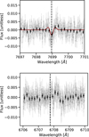 |
Fig. D.1 Transmission spectrum of potassium (top) and lithium (bottom). The black dashed line marks the line position; the solid red line shows the no-atmosphere POLD model (top panel only) to illustrate the deformation scale; the red dashed line shows the continuum (bottom panel only). Gray data points indicate the full transmission spectrum, with black bins every 15 pixels. Potassium is contaminated by POLD effects, with no obvious atmospheric detection. Lithium shows no detection, even though it is not contaminated by POLD effects, as this species does not absorb in the stellar spectrum. |
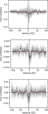 |
Fig. D.2 Velocity folded transmission spectrum of calcium (top), magnesium (middle) and manganese (bottom). The black dashed line is the 0 velocity, with the red dashed line being the continuum. Gray data points full transmission spectrum, with black bins by 15x pixels. Strong POLDs contamination detected with no obvious signal. |
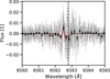 |
Fig. E.1 Fit of the double Gaussian to the RM+CLV corrected transmission spectra at the region of H α. |
 |
Fig. E.2 Transmission spectra in the region of H α per night as calculated for the “Ingress” data (top) and “Egress” data (bottom). Nights are color coded as blue, orange, and green for night #1, #2 and #3 respectively. The vertical black dashed line corresponds to the laboratory wavelength of H α, with the red dashed line positioned at 6562.5Å, the position of the observed absorption feature. The black dashed horizontal line is the continuum level. Note that the “Egress” data for night #2 does not exist due to the partial transit observations. |
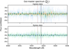 |
Fig. E.3 Out of transit spectra in the region of H α per night as calculated for the “Ingress” data (top) and “Egress” data (bottom). Nights are color coded as blue, orange, and green for night #1, #2 and #3 respectively. The vertical black dashed line corresponds to the laboratory wavelength of H α, with the red dashed line positioned at 6562.5Å, the position of the observed absorption feature. The black dashed horizontal line is the continuum level. Note the “Ingress” data for night #1 consists of 3 spectra, which decreases the observed S/N. |
All Tables
Upper limits for Na I and H α with the corresponding height in planetary radii in parentheses.
All Figures
|
Fig. 1 Location of WASP-31b (red point) in radius versus insolation flux diagram of known exoplanets (small black points), zoomed-in on the hot-Jupiter region. Extracted from NASA Exoplanet archive on 24 March, 2025. |
| In the text | |
|
Fig. 2 Radial-velocity observations of ESPRESSO data. The Rossiter-McLaughlin anomaly is visible, showing the typical signature of an aligned planet as previously deduced by Brown et al. (2012) using a single HARPS transit. Nights are color-coded separately in blue (night #1), orange (#2), and green (#3). |
| In the text | |
|
Fig. 3 Observed simultaneous photometric light curves (top panels) from ECAM for the three ESPRESSO nights. The best-fit models from CONAN for each night are color-coded separately in blue (night #1), orange (#2), and green (#3). The residuals for each night are shown in the bottom panel with an offset. The horizontal line is the continuum of 0. |
| In the text | |
|
Fig. 4 Intrinsic CCF per night (left panels) and their respective residuals (right panels). The RM signature is well visible during the transit as a bright track. The dashed horizontal lines correspond to T14 contact points (orange) and T23 (green). The solid red lines (with black outlines) correspond to spectra that were excluded from the analysis. The dotted black lines correspond to the expected local stellar velocity using the best-fit model. The first night’s residuals show a systematic trend, likely due to line asymmetry. |
| In the text | |
|
Fig. 5 Final posterior corner plot of e revolutions analysis of RM anomaly. All values are well-defined, with an anticorrelation between the contrast and FWHM of the line profile. The contours show 1σ, a region containing 50% of accepted steps and 2σ levels, as defined by the corner package. The solid lines correspond to the median value of the posterior distribution function, which is used as the measured value. |
| In the text | |
|
Fig. 6 Correction for fiber B and telluric lines in the region of the sodium doublet. Each panel shows a respective night, with the master of raw spectra from fiber A (uncorrected for fiber B and telluric lines) in orange. In green, we show the master of fiber A spectra corrected for fiber B and telluric lines. The respective average telluric profile and fiber-B emission are shown in blue and gray, respectively. Please note that fiber B is on an arbitrary scale due to normalization. The zoomed-in image of the inset focuses on the wavelength region of 5890–5891 Å. |
| In the text | |
|
Fig. 7 Same as Figure 6, but in region of H α. No strong telluric features were detected in this region. |
| In the text | |
|
Fig. 8 Combined transmission spectrum and its residuals of WASP-31b in the region of sodium doublet (top panels), and Balmer alpha line (bottom panels) in the rest frame of the planet. We plot the full spectrum in gray; that binned by 15x is shown in black. In this notation, absorption goes above zero, and “emission” is below. The laboratory position of the respective lines is shown via dashed black lines. The no-atmosphere model from EvE is plotted as an orange line, and the compound model with the atmosphere is shown as a green line. The vertical dashed green lines correspond to the escape velocity of ≈33 km/s, centered on the feature at 6562.5Å. The instrumental response function of ESPRESSO is centered on this feature in blue. Residuals were calculated assuming the no-atmosphere model. |
| In the text | |
|
Fig. 9 Phase-resolved cross-correlation of iron template with the dataset of WASP-31b, in the rest frame of the star. Each panel corresponds to a separate night (top panel for first night, middle for second, and bottom for third night). The contact points T1–T4 are plotted as red horizontal dashed lines, with contact points T2–T3 shown as horizontal dashed green lines. The planetary track is shown as a dashed line blue for the out-of-transit section. Absorption features are shown in red (positive) and negative features in blue. |
| In the text | |
|
Fig. 10 Cross-correlation of iron template with the combined and night-specific transmission spectroscopy in the rest frame of the planet. The combined CCF of all nights is shown in black, with the nights shown separately in blue (night 1), orange (night 2), and green (night 3). The top panel shows the full velocity range over which the CCF was calculated. The bottom panel shows a zoomed-in view of −50,50 km s−1. Absorption is positive with respect to the continuum. |
| In the text | |
|
Fig. 11 Chromium-hydride (CrH) cross-correlation search and sensitivity check. The bottom panel shows the phase-folded Kp-Vsys signal-to-noise map of the ESPRESSO WASP-31b transit data cross-correlated with a CrH model template. The dashed lines denote the expected values of (Vsys = −0.1 km s−1, and Kp = 148.0 km s−1, Gaia Collaboration 2023; Flagg et al. 2023). The top panel shows a one-dimensional slice at the expected Kp (along the horizontal dashed white line) for both the data alone (blue) and the data with an injected model (orange). The difference between the blue and orange lines is a measure of the data sensitivity to an underlying signal. In this case, these data only have limited sensitivity to CrH, which has its strongest opacity band heads redward of the ESPRESSO wavelength coverage. Although no clear CrH signal is observed in the data here, we cannot conclusively confirm or rule out its presence in the atmosphere of WASP-31b due to limited sensitivity. |
| In the text | |
|
Fig. 12 Detections (blue) and non-detections (orange) of Na I doublet lines using high-resolution spectrographs based on projected spin-orbit angles (λ) of the system. The green point is the position of WASP-31 b found using our observed values for λ. The top panel shows the (non-)detections with respect to V magnitude. The bottom panel shows the (non-)detections with respect to Teff of the host star. Data were extracted on 7 March, 2025. Although sodium detections exist spanning vastly different orbital alignments, non-detections show a clear preference for aligned systems (1st and 3rd quadrants); however, given the small number of non-detection publications and the higher chance of close-in giants being aligned, we cannot distinguish them from observational bias. |
| In the text | |
|
Fig. A.1 Observation log of the three nights ESPRESSO observation. The red, yellow and green regions correspond to out-of-transit, partial-transit and full-transit phases, with the transit contact points plotted as gray (T1, T4) or black (T2, T3) dotted lines. The blue, orange and green points corresponds to first, second and third night, respectively. Top panel is showing the Airmass variation for each night in the phase space. Middle panel is the same plot but for seeing variation, and bottom panel is the average S/N during the observations. The quality of nights is comparable for the ESPRESSO nights. During the second night (orange points) of ESPRESSO, the seeing condition got worse mid-transit, which led to stopping the observation. |
| In the text | |
|
Fig. B.1 RV curve based on ephemeris provided by Kokori et al. (2023) (top) and Patel & Espinoza (2022) (bottom). The two nights are visually horizontally well aligned in the top panel, while there is clear misalignment in the bottom panel. For visual purposes, only night 1 (blue) and night 3 (green) are plotted. Contact points are plotted as dashed vertical lines in black. RV are corrected for the stellar velocity induced by the planet. |
| In the text | |
|
Fig. C.1 Posteriors distribution of the analysis of intrinsic CCF’s. The top panel shows the center of the Gaussian, the middle panel is the amplitude (contrast) of the Gaussian and the bottom panel is the FWHM. The distributions are color-coded by night (blue for #1, orange for #2 and green for #3). The label corresponds to a specific index assigned to each spectrum at the start of the pipeline, after the spectrum list has been sorted by time (meaning these are phases sorted per night). Only in-transit data are shown (between T1 and T4 contact points). As we use this plot only for illustration of how well/poorly defined the PDFs are, the x and y-axis ticks were removed. The distributions are well-behaved for all spectra during the full transit, but as expected, the first and last transiting spectrum show poorly defined distributions, and were thus removed from the analysis. Furthermore, the second spectrum in second night (#49) shows poor FWHM distribution, and has also been removed from the analysis. |
| In the text | |
|
Fig. C.2 Contrast of the raw CCF, extracted by fitting a Gaussian profile. Each night is color-coded (blue, orange, and green for first, second and third night, respectively). The first few in-transit exposures of the first night are clearly deviating from the trend. The red, yellow and green regions correspond to out-of-transit, partial-transit and full-transit times, with the transit contact points plotted as gray (T1,T4) or black (T2, T3) dotted lines. |
| In the text | |
|
Fig. D.1 Transmission spectrum of potassium (top) and lithium (bottom). The black dashed line marks the line position; the solid red line shows the no-atmosphere POLD model (top panel only) to illustrate the deformation scale; the red dashed line shows the continuum (bottom panel only). Gray data points indicate the full transmission spectrum, with black bins every 15 pixels. Potassium is contaminated by POLD effects, with no obvious atmospheric detection. Lithium shows no detection, even though it is not contaminated by POLD effects, as this species does not absorb in the stellar spectrum. |
| In the text | |
|
Fig. D.2 Velocity folded transmission spectrum of calcium (top), magnesium (middle) and manganese (bottom). The black dashed line is the 0 velocity, with the red dashed line being the continuum. Gray data points full transmission spectrum, with black bins by 15x pixels. Strong POLDs contamination detected with no obvious signal. |
| In the text | |
|
Fig. E.1 Fit of the double Gaussian to the RM+CLV corrected transmission spectra at the region of H α. |
| In the text | |
|
Fig. E.2 Transmission spectra in the region of H α per night as calculated for the “Ingress” data (top) and “Egress” data (bottom). Nights are color coded as blue, orange, and green for night #1, #2 and #3 respectively. The vertical black dashed line corresponds to the laboratory wavelength of H α, with the red dashed line positioned at 6562.5Å, the position of the observed absorption feature. The black dashed horizontal line is the continuum level. Note that the “Egress” data for night #2 does not exist due to the partial transit observations. |
| In the text | |
|
Fig. E.3 Out of transit spectra in the region of H α per night as calculated for the “Ingress” data (top) and “Egress” data (bottom). Nights are color coded as blue, orange, and green for night #1, #2 and #3 respectively. The vertical black dashed line corresponds to the laboratory wavelength of H α, with the red dashed line positioned at 6562.5Å, the position of the observed absorption feature. The black dashed horizontal line is the continuum level. Note the “Ingress” data for night #1 consists of 3 spectra, which decreases the observed S/N. |
| In the text | |
Current usage metrics show cumulative count of Article Views (full-text article views including HTML views, PDF and ePub downloads, according to the available data) and Abstracts Views on Vision4Press platform.
Data correspond to usage on the plateform after 2015. The current usage metrics is available 48-96 hours after online publication and is updated daily on week days.
Initial download of the metrics may take a while.