| Issue |
A&A
Volume 708, April 2026
|
|
|---|---|---|
| Article Number | A214 | |
| Number of page(s) | 45 | |
| Section | Extragalactic astronomy | |
| DOI | https://doi.org/10.1051/0004-6361/202557875 | |
| Published online | 08 April 2026 | |
First statistical constraints on galactic-scale outflow properties traced by their extended Mg II emission with MUSE
1
Leibniz-Institut for Astrophysik Potsdam (AIP), An der Sternwarte 16, 14482 Potsdam, Germany
2
Univ of Lyon1, Ens de Lyon, CNRS, Centre de Recherche Astrophysique de Lyon (CRAL) UMR5574, F-69230 Saint- Genis-Laval, France
3
NSF’s National Optical-Infrared Astronomy Research Laboratory, 950 N. Cherry Ave., Tucson, AZ 85719, USA
4
Department of General Systems Studies, Graduate School of Arts and Sciences, The University of Tokyo, 3-8-1 Komaba, Meguro-ku, Tokyo 153-8902, Japan
★ Corresponding author: This email address is being protected from spambots. You need JavaScript enabled to view it.
Received:
28
October
2025
Accepted:
10
February
2026
Abstract
Galaxies evolve within vast gaseous halos that fuel star formation and carry signatures of feedback-driven outflows. Deep integral field data have enabled the study of Mg IIλλ2796, 2803 halos, which trace galaxy-scale outflows in emission, and while individual detections of Mg II halos have revealed extended circumgalactic structures, their faintness has limited studies to single-object analyses. Here, we present the first statistical study of Mg II-emitting halos using deep MUSE observations of 47 star-forming galaxies at 0.7 < z < 2.0. Building on our previous work, where we developed and applied an outflow modeling framework to a single Mg II halo, we now extend this approach to a larger sample, enabling robust population-level insights into the properties of circumgalactic outflows traced by their extended Mg II emission for the first time. We detected extended Mg II emission out to tens of kiloparsecs and modeled the outflows as an ensemble of radially accelerating shells. Galaxies with Mg II outflows tend to have higher star formation rates (SFRs) and specific star formation rates (sSFRs) and younger stellar populations–consistent with star-formation-driven winds. The observations are consistent with winds that accelerate linearly with radius (v ∝ r) from launching velocities of v ∼ 60 km s−1 up to maximum velocities that correlate with the stellar mass of galaxies, and are of about ∼490 km s−1. The inner regions of the outflows are highly opaque (log τ ∼ 2.6), and we also identify a tentative trend between stellar mass and central optical depth. The opening angle of the outflow shows some dependency on the host-galaxy stellar mass, with less massive galaxies showing primarily wide opening angles (i.e., nearly isotropic outflows), and more massive galaxies showing a broader range of values, with both wide and narrow opening angles. The distribution of the spatial extent of Mg II halos exhibits a clear peak at half-light radius (HLR) of ∼5 kpc, with an extended tail of larger HLR values, up to ∼20 kpc. Compact halo sizes (HLR < 8 kpc) correlate with stellar mass, but extended halos do not, which could suggest a difference in the powering mechanism between compact and extended halos. This work provides new insight into the structure and dynamics of the circumgalactic medium and its role in galaxy evolution by constraining, for the first time, the properties of circumgalactic outflows with a statistically significant sample of galaxies with an extended Mg II emission halo.
Key words: galaxies: evolution / galaxies: general / galaxies: halos / galaxies: structure
© The Authors 2026
 Open Access article, published by EDP Sciences, under the terms of the Creative Commons Attribution License (https://creativecommons.org/licenses/by/4.0), which permits unrestricted use, distribution, and reproduction in any medium, provided the original work is properly cited.
This article is published in open access under the Subscribe to Open model. This email address is being protected from spambots. You need JavaScript enabled to view it. to support open access publication.
1. Introduction
Observing galactic halos in emission poses a major challenge due to the low densities of the gas within them (on the order of nH ∼ 10−4 cm−3; see, e.g., Werk et al. 2014). At high redshifts (z > 3), long exposure time integral field data have enabled the detection and characterization of individual galactic halos probed by their Lyα emission (e.g., Wisotzki et al. 2016; Leclercq et al. 2017; Kusakabe et al. 2022; Erb et al. 2023). These Lyα halos are typically ten times larger in scale length than the stellar component of their host galaxies (Leclercq et al. 2017; Wisotzki et al. 2016), and several studies have indicated that they originate from the resonant scattering of photons produced by the central galaxy with neutral hydrogen atoms in the circumgalactic medium (CGM; e.g., Kusakabe et al. 2019; Song et al. 2020; Byrohl & Gronke 2020). For this reason, the complex spectral profiles and morphologies observed in the Lyα halos carry crucial information about outflows and inflows (i.e., baryon cycle) taking place in these galaxies (Erb et al. 2018; Remolina-Gutiérrez & Forero-Romero 2019; Mitchell et al. 2021).
However, given that Lyα is in the rest-frame UV spectrum of galaxies, in lower-redshift galaxies (z < 3), it is inaccessible from ground-based observing facilities. The Mg IIλλ2796, 2803 doublet provides an alternative resonant line that, similar to Lyα, allows photons to scatter off ions in the CGM, but it is accessible at lower redshifts. It is one of the most abundant metal ions in the Universe, and it has an ionization potential slightly lower than that of hydrogen, making it a good tracer of the cool (T ∼ 104 K) phase of the CGM. Unlike Lyα, which originates primarily from recombination in H II regions powered by young massive stars, Mg II halos are predominantly produced through the scattering of stellar continuum photons (e.g., Prochaska et al. 2011). Other alternative tracers of the cool gas in the CGM used in previous works are provided by the fluorescent FeII* (e.g., Finley et al. 2017a,b) and SiII* (Kusakabe et al. 2024) emission lines. However, these lines are weaker and lie at bluer wavelengths than Mg II.
The first detection of extended Mg II emission around a galaxy was reported by Rubin et al. (2011), using slit-spectroscopy. They found an excess of Mg II emission with respect to the stellar continuum around a galaxy at z = 0.69 out to distances of ∼10 kpc from the central galaxy. This emission is interpreted as ions present in outflows scattering with photons produced by the central galaxy. The same object was later observed using Keck Cosmic Web Imager integral field spectroscopy (Burchett et al. 2021), which enabled study of the extended Mg II emission in a spatially resolved manner, and compared with the radiative transfer models from Prochaska et al. (2011) to infer the physical properties of the outflow, such as orientation and velocity profile. The data was found to be consistent with an isotropic and radially decelerating wind.
Another example of such spatially resolved studies is Zabl et al. (2021), where the authors used the unique capabilities, in terms of angular resolution and sensitivity, of the Multi-Unit Spectroscopic Explorer (MUSE, Bacon et al. 2010) to study the extended Mg II emission up to distances of ∼25 kpc from a galaxy at z = 0.7, whose CGM was also probed in absorption by a quasi-stellar object sight line at an impact parameter of ∼39 kpc. They found their data to be consistent with the expectation from a simple toy model of a biconical outflow with a constant slow velocity (130 km s−1). Leclercq et al. (2022) also used MUSE data from the MUSE eXtremely Deep Field (MXDF; Bacon et al. 2017, 2023) and reported the discovery of extended Mg II emission emerging from the intragroup medium of a group of five star-forming galaxies at z = 1.31 and concluded that the intragroup medium is enriched by both outflows and tidal stripping from galaxy interactions. More recently, Pessa et al. (2024) have reported the discovery of an extended Mg II halo around a star-forming galaxy at z ∼ 0.7 in the MUSE Hubble Ultra Deep Field mosaic (Bacon et al. 2017, 2023), with Mg II emission present up to distances of 30–40 kpc from the central galaxy. The authors found that the observed emission is consistent with radially accelerating winds.
Due to the intrinsic difficulty of studying the CGM in emission, primarily because of its low density, the detections of extended Mg II emission in individual galaxies listed previously have relied on very deep MUSE observations (10 − 140 hrs). These studies have revealed detailed morphologies and kinematic structures in single objects, highlighting the power of integral field spectroscopy for resolving the CGM of individual galaxies.
In addition to these individual studies, stacked analyses have enabled the detection of extended Mg II halos in a statistical sense by enhancing the low surface brightness signal Guo et al. (2023), Dutta et al. (2023). Guo et al. (2023) stacked MUSE data cube segments for 172 galaxies from the MUSE Hubble Ultra Deep Field surveys and identified a significant enhancement of Mg II emission along the minor axis, consistent with bipolar outflows, extending beyond 10 kpc. This finding contrasts with the results from Dutta et al. (2023), where the authors stacked the Mg II emission of nearly 40 galaxies from the MUSE Ultra Deep Field survey (MUDF; Fossati et al. 2019) and found no significant difference between the major and minor axes. However, stacking inherently averages over diverse morphologies and environments, thus limiting one’s ability to study the specific characteristics of individual systems.
Deep observations of individual galaxies and stacked analyses have both played crucial roles in advancing our understanding of extended Mg II emission. Individual detections have revealed the detailed morphologies, orientations, and kinematic features of Mg II halos, offering insight into the physical mechanisms at play in specific systems. In contrast, stacked studies have demonstrated the ubiquity of such emission on average, confirming the presence of diffuse Mg II halos across galaxy populations, However, despite these important contributions, neither approach alone provides a statistical baseline to study the properties of the Mg II halos on a population level and how their properties depend on the host-galaxy properties. Thus, transitioning to sample-level analyses is paramount to understanding the complex interplay between galaxies and their CGM.
Sample-level analyses involve studying in a comparable manner the properties of a collection of objects rather than focusing on the properties of a single galaxy, often chosen due to its special properties, rather than being a representative case. In this paper, we use deep MUSE data to build, for the first time, a sample of galaxies with extended Mg II emission and study the properties of Mg II halos on a population level, going beyond single-object discoveries. We used the outflow model introduced in Pessa et al. (2024) to infer the physical properties of the galactic winds shaping these Mg II halos, and we explored correlations between host galaxies and outflow properties. The paper is structured as follows. In Sec. 2, we present our data, and in Sec. 3, we describe our sample selection and the general properties of our sample galaxies. In Sec. 4 we present the size distribution of the Mg II halos in our sample, and in Sec. 5, we show the results of fitting our outflow model to the sample galaxies. In Sec. 6, we discuss the implications of our results and compare the physical properties of our sample galaxies to those inferred for their galactic winds. Finally, in Sec. 7, we summarize our findings and conclusions. In Appendix E, we describe some of the relevant aspects of the methodology employed for our analyses, including a description of the outflow model used in Appendix E.1. We used a flat concordance cosmological model with H0 = 70 km s−1 Mpc−1 and Ωm = 0.3. All quoted transverse distances are in physical units, not comoving.
2. Observational data
2.1. MUSCATEL survey
The MUSE Cosmic Assembly survey Targeting Extragalactic Legacy fields (MUSCATEL; PIs: Lutz Wisotzki, Roland Bacon, Thierry Contini) is based on observations with the MUSE instrument on the ESO-VLT (Bacon et al. 2010). MUSE is a panoramic integral-field spectrograph with a field of view of 1′×1′ (in Wide Field Mode, used for these observations) at a spatial sampling of  . The spectral range is 4700 Å–9350 Å, with a spectral sampling of 1.25 Å and a wavelength-dependent velocity resolution between ∼190 and ∼80 km s−1 (full width at half maximum; FWHM) at the blue and red ends of the spectrum, respectively.
The MUSCATEL survey consists of MUSE observations of parallel fields of the Hubble Frontier Fields (HFF, Pagul et al. 2021), for 4 clusters accessible to the VLT (A2744, M0416, AS1063, A370). We employed a wedding cake approach for the observing strategy, with three different levels of exposure time. First, a large shallow field composed of a 3′×3′ mosaic of 100 min exposure time following the Hubble Space Telescope (HST) Advanced Camera for Surveys (ACS) footprint of the parallel fields. Then, the medium field lies on top of the shallow field, consisting of a 2′×2′ mosaic of 5 hours depth, following the HST Wide Field Camera 3 (WFC3) footprint. Finally, the deep field consists of a single 1′×1′ MUSE pointing on top of the medium field, with 25 hours of observing time and a suitable star for the PSF characterization1.
Some of the science goals of the MUSCATEL survey include increasing the number of deep fields, reducing cosmic variance, and improving statistics for studies that require deep data (e.g., clustering). All the observations have been carried out using the VLT adaptive optics facility (AO, Leibundgut et al. 2017), with the exception of one of the shallow field pointings from the AS1063 clusters, and a small number of additional individual exposures. The separation from the parallel fields to the center of the clusters is large (6 arcmin), meaning that the parallel fields are not affected by gravitational lensing from cluster galaxies. Furthermore, excluding redshifts consistent with the cluster, the redshift distribution of galaxies in the field is consistent with those from other deep fields.
We have proceeded with the data reduction in a similar way as Urrutia et al. (2019), using the standard MUSE data reduction software (Weilbacher et al. 2014, 2020), but with additional post-processing steps, for instance, superflat correction as described in Bacon et al. (2023). We have then used the LSDCat software (Line Source Detection and Cataloguing, Herenz & Wisotzki 2017) to search for emission line peaks in the MUSCATEL reduced data cubes. We have imposed a S/N threshold in the emission line of 5 to get rid of spurious sources2, and created a catalog of emission-line-selected galaxies, for which we have carried out a careful supervised redshift determination. The final catalog contains a total of 3245 galaxies with a measured redshift. The details of the redshift determination, the construction of the galaxy catalog, as well as other critical aspects of the MUSCATEL survey, such as an exhaustive description of the data and data reduction will be reported in a future MUSCATEL dedicated survey paper.
2.2. Photometric data
In addition to the MUSE observations, there is extensive multiwavelength photometric archival data available for the fields targeted by the MUSCATEL survey. In particular, deep optical and near-infrared images were obtained with the Hubble Space Telescope (HST, Shipley et al. 2018; Pagul et al. 2021). The optical bands available include the F435W, F606W, and F814W bands from the HST/ACS. The NIR bands include the F105W, F125W, F140W, and F160W bands from the HST/WFC3. There is also available deep James Webb Space Telescope (JWST) data for these fields (e.g, Bezanson et al. 2024; Rihtaršič et al. 2025). However, these data are currently still undergoing postprocessing; thus, we do not use them in this work.
For each galaxy in the catalog of emission-line-selected galaxies, we have identified its counterpart in the HST images and used the photometric data to perform a fitting of its spectral energy distribution (SED). We estimated the stellar mass, star formation rate (SFR), and age of each galaxy by fitting the broad-band SED with the FAST code (Kriek et al. 2009), employing all available HST photometric bands, and the models from the Bruzual & Charlot (2003) stellar library, assuming a Chabrier IMF (Chabrier 2003) and an exponentially declining star formation history. We use four possible stellar metallicities to fit the data, namely Z = [0.004, 0.008, 0.02, 0.05]. The uncertainties in stellar mass, SFR, and age were estimated by performing 300 Monte Carlo iterations, and are on the order of 0.2, 0.3, and 0.2 dex, respectively. The SED fitting also yielded a global estimate of the dust extinction acting on the starlight, assuming a Calzetti et al. (2000) extinction curve. The stellar masses, SFRs, and ages computed via SED fitting for each galaxy are provided in Table D.1.
The counterpart identification is carried out by cross-matching the location of the galaxies identified in the MUSCATEL dataset with the objects in the HST catalogs. A subsequent visual inspection ensured the consistency of the identifications. Since the galaxies in our sample are relatively continuum bright3, there is little ambiguity in the counterpart identification. For only one of our sample galaxies, we were not able to unambiguously determine its HST counterpart, due to the crowded field and irregular morphology of the galaxies near the MUSE detection (see caption of Table D.1).
3. Galaxy sample
3.1. Sample selection
Our goal is to build a sample of galaxies where we can robustly detect extended Mg II outflow emission and measure its properties. However, designing a selection criterion for this purpose is not straightforward. A simple flux threshold in the Mg II line could potentially be misleading, depending on the geometry of the outflow and the size of the galaxy. The spectrum extracted from a fixed-size aperture could be, for instance, strongly dominated by Mg II in absorption, with the emission present at larger impact parameters. Another possibility is that the emission and absorption components partially or totally cancel out each other, biasing the strength of the Mg II emission in the aperture-integrated spectrum. On the other hand, a minimum S/N threshold in the stellar continuum emission might also be suboptimal since it would not be informative about the relative strength of the Mg II emission with respect to the continuum. Additionally, it would also imply indirectly imposing a stellar mass limit in our sample, and the work from Feltre et al. (2018) shows that there is a correlation between the observed Mg II spectral profile and galaxy stellar mass, where most massive galaxies are more likely to show Mg II in absorption, and less massive galaxies show mostly Mg II in emission.
Thus, we opted for the following approach. First, we kept only those galaxies in the MUSCATEL catalog within the redshift range where the Mg II doublet is available in the MUSE wavelength range, that is, 0.7 ≲ z ≲ 2.3, and with redshift confidence of 3 (i.e., a secure redshift determination based on more than one spectral feature). This leaves us with an initial sample of 545 galaxies. Hereafter, we refer to this sample as our parent sample.
Then, we visually inspected the aperture-integrated spectrum of each source (in an aperture of angular size  , approximately 82 kpc2 at z = 1), as well as their continuum-subtracted Mg II pseudo-narrowband image constructed from a cutout of the MUSE data cube around the Mg II doublet wavelength (2790 − 2810 Å in the rest-frame of each galaxy). We kept the galaxies where we found evidence of Mg II emission or absorption in the integrated spectrum or in the continuum-subtracted pseudo-narrowband image without imposing a priori any S/N threshold.
We ended up with a sample of 89 galaxies, which we refer to as our preliminary sample. Next, we examined their spectra in concentric annular apertures ( ,
,  ,
,  ,
,  ,
,  , which correspond to physical impact parameters of r < 3.2 kpc, 3.2 kpc < r < 6.4 kpc, 6.4 kpc < r < 9.6 kpc, 9.6 kpc < r < 16.0 kpc, 16.0 kpc < r < 28.0 kpc at z = 1), and classified the Mg II profiles of the sample galaxies as P-Cygni (Pcyg), absorption-only (Abs), and emission-only (Ems), depending on whether they show clear Mg II absorption and/or emission along these radial apertures. For instance, for some galaxies, their integrated spectrum in a circular aperture could be dominated by Mg II in emission, but if they exhibit Mg II in absorption in an inner, smaller aperture, they were classified as a P-Cygni profile. Inspecting the spectra of galaxies in radial apertures is thus useful for disentangling strong central absorption from Mg II emission at larger radii. The profile classification has been done in a qualitative manner, based on the presence of significant absorption and/or emission in the spectra extracted from annular apertures.
Figure 1 shows the stellar mass distribution (computed from the SED fitting; see Sec. 2.2 for details) of the galaxies in our preliminary sample, separated by MUSCATEL depth and profile type. Our sample is consistent with the findings from Feltre et al. (2018), where galaxies that show Mg II in absorption are generally on the high-mass side of the distribution, galaxies that show Mg II in emission lie generally on the lower-mass side, whereas galaxies that exhibit a P-Cygni profile lie somewhere in between (albeit the stellar mass range of our sample galaxies is narrower than that of Feltre et al. (2018), and thus the correlation of spectral profile and stellar mass is less evident here).
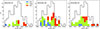 |
Fig. 1. Stellar mass distribution of our preliminary sample of galaxies. The sample consists of 89 galaxies drawn from the MUSCATEL survey that exhibit Mg II in emission or absorption or a P-Cygni profile, determined after a careful inspection of their integrated spectra and their continuum-subtracted Mg II pseudo-narrowband image. A direct S/N threshold has not been applied. Each stacked histogram shows the distribution of the galaxies that belong to each one of the depth levels of the MUSCATEL survey (shallow field, medium field, and deep field; see Sec. 2), indicated in the top-left part of each panel. The black line shows the distribution of the full preliminary sample in all the panels. Stellar masses are calculated via SED fitting, as described in Sec. 2.2. The stacked histograms are color coded by the different spectral profiles shown in Mg II, as indicated in the legend. |
From the preliminary sample, we then opted to keep only those galaxies that show a P-Cygni profile in Mg II, since this feature is interpreted as a signature of resonant scattering in an optically thick outflow, with absorption in the approaching (blueshifted) regions of the outflow and a redshifted emission component due to backscattering in the receding material (e.g., Castor 1970; Castor & Lamers 1979; Scuderi et al. 1992). This clear outflow signature makes them more suitable for studying the physical properties of galactic winds. Out of the 89 galaxies in the preliminary sample, 50 show a clear P-Cygni profile. However, we stress that while the non-P-Cygni galaxies will be excluded from the analyses carried out in this paper, we will include them in our sample in a future paper, where we will investigate the properties of this broader halo population.
3.2. Mg II significance
We then used our outflow modeling scheme to model the MUSE data cube cutout of each one of the P-Cygni galaxies. Our outflow model is described in detail in Pessa et al. (2024). In Appendix E.1 we include a summarized description of the model. At this stage, we used our model only to reproduce the spectral profile of the Mg II absorption. By modeling the absorption of the photons produced by the central source, we were able to correct for it (i.e., add the flux from the absorbed photons back into the observed spectra), and then produce a Mg II emission-only data cube for each galaxy. We disentangle the Mg II emission from the absorption in order to quantify the significance of the Mg II emission.
We stress that the model was only used to reproduce the absorption profile at this point. The actual best-fitting parameters, or the performance of the model at reproducing the extended emission, are not relevant here. In principle, we could use different methods to perform this correction (e.g., optical depth and covering fractions that vary as a function of projected velocity; see Xu et al. 2022). Still, for internal consistency, we opted to use the same model that we later use to infer the properties of the galactic winds.
Next, we produced a continuum cube for each galaxy and removed the continuum from the Mg II emission-only (already absorption corrected) data cube. The continuum cubes were constructed using a running median across the spectral dimension of the original cube, within a window of 200 wavelength channels.
We then collapsed the continuum-subtracted Mg II emission-only data cubes along the wavelength axis (using a mean) to produce an emission-only continuum-subtracted Mg II pseudo-narrowband image, for a wavelength range of approximately 2790 Å < λ < 2809 Å rest-frame (this range can be slightly different for some galaxies if they exhibit, for instance, a broader spectral profile, or contamination due to a nearby sky emission line, as detailed in Appendix E.2.2). We used this pseudo-narrowband image to compute the S/N of the Mg II emission for each galaxy. We computed the S/N of each galaxy in two different ways. First, we simply integrated the Mg II flux across the full modeled region (a circular aperture of  radius; see Appendix E.2.2) and divided it by the square root of the integrated variance across the same region. Secondly, we did the same calculation, but for the different annular apertures defined earlier at the beginning of this section separately, and we kept the highest S/N among the different apertures (excluding the central one, in order to minimize the contribution from nebular emission and focus on the extended component). We finally opted to use the highest of the two different values (integrated in the whole modeled region versus integrated in an annular aperture). The motivation behind this criterion is that while some halos are more spatially extended, and integrating over larger apertures maximizes the significance of the Mg II emission, others are more compact and radially concentrated. For the latter, integrating over large apertures leads to a dilution of the total signal. We did not aim at discarding some halo morphologies with our selection criterion; thus, we used this flexible definition to characterize the significance of the Mg II emission.
After calculating the S/N of each galaxy, we kept in our sample only those galaxies with a mean S/N (wavelength averaged) higher than 3. The left panel of Fig. 2 shows the distribution of the S/N values for our sample galaxies. Out of the 50 galaxies that show a P-Cygni profile, 47 present a S/N above the minimum significance threshold of 3σ, and we deem these galaxies to be robust detections of extended Mg II halos tracing galactic-scale outflows. These 47 galaxies form our final sample. 22 of these galaxies are drawn from the MUSCATEL deep field, 17 from the medium field, and 8 from the shallow field (see Sec. 2).
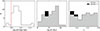 |
Fig. 2. Significance of the extended Mg II emission, stellar mass, and redshift distribution for the galaxies in our preliminary sample that exhibit a P-Cygni profile in Mg II. Left: significance of the extended Mg II emission in terms of its spatially integrated S/N for the 50 galaxies in our preliminary sample that exhibit a P-Cygni profile in Mg II. We further removed from our preliminary sample those galaxies where the integrated S/N of the modeled emission is lower than 3σ (indicated with a vertical dashed red line). Middle: stacked histogram that shows the stellar mass distribution of galaxies in the preliminary sample with a P-Cygni profile in Mg II. The gray histogram shows the stellar mass distribution of those galaxies where the significance of the Mg II emission is above the 3σ threshold. The black histogram shows the stellar mass distribution of galaxies below this significance threshold. Right: same as middle panel, but for the redshift distribution of the sample galaxies. |
While our objective is to search for primarily extended Mg II halos (hence, we excluded the central aperture from the annular apertures), we do not filter our sample by halo size at this stage, that is, our sample could potentially include galaxies for which the size of the Mg II emission is consistent with the size of their continuum counterpart. However, even if this is the case, the observed light distribution of Mg II will always be different from the continuum light distribution, because, by construction, all the galaxies in our final sample exhibit some level of Mg II absorption in their central region. Furthermore, due to the generally irregular morphology of the Mg II halos, parameterizing their sizes is not straightforward. In Secs. 4 and 6.3 we present and discuss the size of the Mg II emission of our sample galaxies in detail and compare these sizes with the size of their continuum counterpart.
The middle panel of Fig. 2 shows the stellar mass distribution for the galaxies above and below the significance threshold. Galaxies with lower Mg II S/N are preferentially on the low-mass half of the distribution, with stellar masses of log M* ∼ 8.8 M⊙ (although still close to the median of the distribution of log M* = 9.2 M⊙). The right panel of the figure shows the redshift distribution for galaxies above and below our S/N threshold. The galaxies below our S/N threshold are all at z < 1. Our final sample presents a relatively flat redshift distribution. The slightly smaller number of galaxies at z ∼ 1.1 is caused by the AO wavelength gap coinciding with the wavelength of the Mg II doublet at that redshift.
3.3. Sample characterization
Figure 3 shows the SFR versus the stellar mass of the galaxies in our final sample, as well as the rest of the galaxies in our preliminary and parent samples. Both quantities are measured via SED fitting (see Sec. 2.2 for details). Most galaxies in our final sample lie relatively close to the star-forming main sequence (SFMS; see, e.g., Brinchmann et al. 2004; Daddi et al. 2007; Noeske et al. 2007; Popesso et al. 2023). However, there is significant scatter, with some galaxies that exhibit considerably higher and lower SFRs, compared to their expected value, given their stellar mass. This implies that Mg II halos are not necessarily always associated with starbursting galaxies, as previous works could suggest (e.g., Zabl et al. 2021). Indeed, only a small fraction of our sample galaxies could be considered as starbursts, significantly above the SFMS. On the contrary, most of them lie closer to or even below the SFMS.
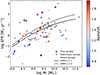 |
Fig. 3. Star formation rate as a function of stellar mass for our sample galaxies. Both quantities were obtained via SED fitting (see Sec. 2.2). Our final sample of 47 galaxies that exhibit a P-Cygni profile and a significant detection of modeled extended emission is shown with squares, color coded by redshift. The preliminary sample is shown as dark gray circles, and the original parent sample is shown as smaller light gray dots. For reference, we show the SFMS as measured by Popesso et al. (2023) for z = 1 (solid) and z = 2 (dashed) by collecting different measurements of the SFMS for a wide range of redshifts. |
Figure 4 shows the continuum-subtracted Mg II pseudo-narrowband image (not corrected by absorption) overlaid onto the HST/F814W images for each galaxy in our final sample, for a square field of view of 40 kpc × 40 kpc. The Mg II emission is shown in black, and the stellar light from the HST data is in blue. The continuum-subtracted pseudo-narrowband images were created by collapsing the continuum-subtracted cubes across their wavelength dimension, for the full modeled wavelength range that encloses the complete P-Cygni profile of both Mg II lines (approximately 2790 Å < λ < 2809 Å rest-frame. The exact modeled wavelength range used for each galaxy is shown in the figures in Appendix B). For visualization purposes only, the continuum-subtracted Mg II pseudo-narrowband images have been smoothed with a Gaussian kernel of  FWHM.
FWHM.
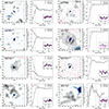 |
Fig. 4. Compilation of continuum-subtracted Mg II pseudo-narrowband images (gray color scale) and HST F814W images (blue color scale, probing the stellar light) for our final sample of galaxies that exhibit a P-Cygni profile in Mg II as well as a significant detection of extended Mg II emission. Galaxies are sorted by stellar mass in descending order. The continuum-subtracted Mg II pseudo-narrowband images were computed by collapsing the MUSE data across the wavelength axis for wavelengths that enclose the full P-Cygni profile of the Mg II doublet for a field of view of 80 × 80 kpc2. The brown circle in the bottom-left part of the panel shows the size of the MUSE PSF. The black contours show the 1-σ and 2-σ detection levels of Mg II net emission in the pseudo-narrowband images. The red contours show the 2-σ and 4-σ levels of Mg II net absorption in the pseudo-narrowband images. For visualization purposes, the continuum-subtracted Mg II pseudo-narrowband images have been smoothed using a Gaussian kernel with a FWHM of 1 arcsec. For each galaxy, we also show the radial profile of the Mg II emission as observed in the data (solid) and after correcting by self-absorption using our best-fitting model (dashed; see Sec. 4). The vertical dotted brown line shows the half-light radius measured for the self-absorption corrected radial profiles. The inset shows the Mg II spectrum extracted from the MUSE data cube for each galaxy, across the full modeled region (black) and a small central aperture of radius |

In many cases, the halos present strong Mg II absorption in the central part, and while some galaxies seem to display only Mg II emission in the pseudo-narrowband, by construction, all of them exhibit some level of absorption (the emission might overcome the absorption when the profile is integrated along the wavelength axis). The figure also shows the observed surface brightness profiles of the Mg II emission, which, for the galaxies that present strong central absorption, are negative at small galactocentric distances. Hereafter, for simplicity, we refer to galaxies in the final sample as our sample galaxies. Table D.1 summarizes the general properties of our sample galaxies.
We acknowledge, however, that our sample selection criteria inevitably lead to biasing our sample in the parameter space of galaxy properties. For instance, by keeping only the galaxies that exhibit a P-Cygni profile in the Mg II line, we are more likely to drop galaxies in the extremes of the mass distribution (see, e.g., Feltre et al. 2018, and Fig. 1). Similarly, by setting a minimum S/N of the Mg II extended emission, we are also dropping preferentially galaxies on the low-mass side of the distribution (see Fig. 2). Additionally, since at a constant total luminosity, more extended halos are less likely to be detected than more compact ones (see, e.g., Pharo et al. 2024, in the context of Lyα halos), this means that we could be excluding from our sample those more extended halos in less massive galaxies. Also, these biases in the sample ultimately mean that we are confined to limited regions in the parameter space and that our conclusions cannot be extended to, for instance, the low- and high-end of the mass distribution.
3.3.1. Independent SFR measurement for our sample galaxies
For galaxies at redshift lower than 1.48, the [O II] λλ3727, 3729 doublet falls comfortably within the MUSE wavelength range, and thus for these galaxies we can compute an independent estimation of their SFR from their [O II] λλ3727, 3729 emission, which traces star formation on timescales of a few megayears.
To compute the SFR values from their [O II] λλ3727, 3729 luminosity, we used the following relation from Kewley et al. (2004):
 (1)
(1)
The spectra of the sample galaxies have been corrected by dust extinction before computing their SFROII, using the extinction derived from the SED fitting (generally, the emission lines will be subject to higher extinction values than the stellar continuum, so this mainly provides a lower limit on the emission line extinction; see, e.g., Hemmati et al. 2015; Emsellem et al. 2022). Also, because of the lack of additional emission lines to perform further diagnosis of the ionization mechanism (e.g., Baldwin–Phillips–Terlevich diagram Baldwin et al. 1981), we assume that all the [O II] emission of these galaxies traces SFR, which might not be entirely true, as some [O II] emission can be produced by other mechanisms such as shock ionization (see, e.g., Reynaldi & Feinstein 2013). Figure 5 shows the comparison of the SFR estimated from the SED fitting with the values determined from the [O II] luminosity for the galaxies where [O II] is available. Despite not accounting for non star-formation ionization, and using the dust extinction derived from the SED fitting, we find that there is a relatively good agreement between both independent estimations, with some higher dispersion for the galaxies on the low-end of the SFR distribution, which is not unexpected because, in addition to the intrinsic random and systematic uncertainties in both measurements, they also trace SFR on different timescales. Table D.1 provides the SFR values measured from the [O II] line for those galaxies where [O II] is available, given their redshift and the MUSE wavelength range (There are no galaxies in our sample at z < 1.48 where the [O II] line is undetected).
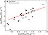 |
Fig. 5. Comparison of the SFR values derived for our sample galaxies obtained via SED fitting (see Sec. 2.2 for details) and from the [O II] luminosity of each galaxy (see Sec. 3.3.1). The black squares show the SFR values for galaxies in our final sample, and the gray dots show the SFR values for galaxies in the preliminary sample, for the subset of galaxies at z ≲ 1.48, where the [O II] doublet falls well within the MUSE wavelength range. The red line shows the identity for reference. Table D.1 provides these measurements for each galaxy in our final sample. |
3.3.2. Comparison of final sample with parent sample galaxies
In this subsection, we compare different properties of our final sample of galaxies derived via SED fitting with those from the original parent sample. Our aim is to study whether there are some peculiarities in our sample galaxies relative to the parent sample. In other words, if there is something special about our sample galaxies that could correlate with the existence of galactic-scale outflows. Figure 6 shows the distribution of stellar mass, SFR, specific SFR (sSFR), and stellar age for our final sample of galaxies, as well as for the original parent sample.
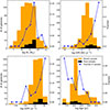 |
Fig. 6. Comparison of the stellar mass, SFR, sSFR, and age distributions for our final sample of galaxies (black) and our parent sample (orange). The blue line shows the fraction of galaxies from the parent sample in our final sample in each bin of the relevant quantity for each panel. The right side y-axis indicates the fraction shown by the blue line. |
In terms of stellar mass, there is no clear preference for our sample galaxies. The fraction of galaxies from the parent sample inside our sample peaks at log M* ∼ 9.5, with a sharp decrease toward higher and lower stellar masses. The sharp declines toward the extremes of the mass distribution could be, at least partially, driven by our preselection of galaxies that exhibit a P-Cygni profile in their Mg II line, which, as discussed earlier in this section, are preferentially associated with galaxies of intermediate stellar masses.
On the other hand, there seems to be some preference in the SFR, sSFR, and age values occupied by our sample galaxies, where the fraction of galaxies included in our sample tends to increase toward higher SFR and sSFR bins (that also correspond to younger age bins). We have performed a Kolmogorov–Smirnov (K–S) test to compare the distributions of our parent and final samples, for the four quantities shown in Fig. 6 in a more quantitative manner. We found that for all of them, the p-value is lower than 0.02, meaning that the distributions are significantly different. This is consistent with the expectations, since galactic-scale outflows on the stellar mass range relevant for our sample are expected to be primarily powered by stellar feedback (Nelson et al. 2019a), and the strength of stellar feedback is directly connected to the galaxy SFR, sSFR, and thus age.
However, even in these high SFR and sSFR and young bins, the fraction of galaxies that present an outflow traced by their Mg II emission is not extremely high (∼20 − 40%), meaning that having a certain SFR, or a certain number of young stars, does not strictly correlate with the presence of cool-gas outflows (although as mentioned in Sec. 3, there could also be outflowing galaxies that do not present a P-Cygni profile, for instance, an edge-on biconical outflow that does not produce central absorption). There must also be other physical conditions required, such as ISM density or temperature. Alternatively, it might also be a matter of timescales, that is, the time when a cool-gas outflow is detectable could be a relatively small window after the last star-forming episode. In a future paper, we will further investigate in more detail different aspects of our sample galaxies, aiming at shedding light on what is fundamentally determining the presence of an outflow in a given galaxy.
We note that our final sample contains galaxies from the three different depth levels of the MUSCATEL survey. Thus, the heterogeneous exposure times could also potentially factor into the fraction of galaxies from the parent sample included in our final sample. Indeed, the total fraction of galaxies in our final sample per depth level is the highest for the deep field (∼14%), and the lowest for the shallow field (∼4%), with the medium field in between (∼9%). However, the trends with the host galaxy properties explored in this section remain the same for the different depth levels, that is, higher fractions for young, star-forming galaxies (albeit with higher scatter, due to the lower statistics when considering individual depth levels only). On the other side, the fraction of galaxies in the youngest and highest star-forming bins from the parent sample in our sample is significantly higher in the deep and medium fields (∼80% in the highest SFR bin, and ∼30 − 40% in the second highest bin, for both deep and medium field, individually), compared to a ∼16% and ∼11% fraction in the highest and second highest SFR bin for the shallow field. Thus, although the dependence on host galaxy properties is robust, the absolute fraction varies significantly for different depth levels (see Appendix F). This is not surprising, and it is the core reason of why previous studies of galactic-scale outflows traced by extended Mg II emission have focused mainly on single-objects analyses, for which deep (> 10 hrs exposure time) integral field data is available (see, e.g., Burchett et al. 2021; Zabl et al. 2021; Leclercq et al. 2022; Pessa et al. 2024) or stacking data (see, e.g., Guo et al. 2023; Dutta et al. 2023).
4. Reconstruction of the Mg II halos
As discussed in Sec. 3, by construction, we built our sample including those galaxies that show both emission and absorption of Mg II in their spectra. This implies that the observed surface brightness profiles of the Mg II emission halos are different from the intrinsic profiles that would be observed if there were no self-absorption of the central source by the halo, meaning that any measurement of size or morphology strongly depends on the geometry and orientation of the halo with respect to the line of sight since face-on outflows will be more affected by central absorption than more edge-on outflows (see, e.g., Guo et al. 2023).
However, as described in Sec. 3, we can use the best-fitting models for each galaxy to correct for the Mg II absorption of the central galaxy spectrum, and then infer the absorption-corrected intrinsic surface brightness profile of the Mg II emission halos. Figure 4 shows both the observed and absorption-corrected surface brightness profiles of the Mg II pseudo-narrowband image. Since, by construction, all the galaxies present some level of central self-absorption, the corrected profile is always brighter in the center than the observed one. The corrected profile is always positive in the central region, with the exception of A2744-DF-013, where the model underestimates the strength of the absorption, and thus, after correcting for absorption, it remains negative (this particular galaxy is discussed in more detail in Appendix C).
Once we corrected for self-absorption, we proceeded to characterize the physical extent of the Mg II halos using their half-light radius (HLR). To minimize the possible contamination by nearby sources, we compute the HLR as the radius at which half of the total Mg II emission within a radius of 30 kpc from the central source is contained. The HLR of each galaxy in our sample is shown as a vertical dotted brown line in the panels that show the surface brightness profiles in Fig. 4, and it is provided in Table D.1. The errors of the HLRs have been computed by performing 100 Monte Carlo iterations, perturbing the radial profile according to the errors of each radial bin, in each iteration. We have used the standard deviation of these 100 iterations as the error of the HLR measurement.
We stress that these HLR values were measured from the MUSE data, and thus they include the contribution from the MUSE PSF. Nevertheless, the Mg II emission of our sample galaxies is generally significantly more extended than the MUSE PSF (see Fig. 4), and thus our measurements are not strongly affected by the PSF contribution. Another caveat of the HLR is that since it is an azimuthally averaged quantity, it is not an optimal metric for non-isotropic configurations. For instance, galaxies such as M0416-MF2-106 and AS1063-MF4-100 exhibit some of the lowest HLRs among our sample galaxies (both of about 3.6 kpc). However, in the corresponding panels of Fig. 4, it is clear that they present an elongated shape whose extent is not properly captured by an azimuthally averaged metric and are somewhat off-center with respect to their stellar counterpart. Due to the difficulties of parameterizing the shape of the observed Mg II halos, we stick to the HLR metric to quantify sizes, as it does provide a useful reference value, but we caution the reader about this caveat.
Figure 7 shows the distribution of the HLRs of the Mg II halos in our sample galaxies. Most galaxies have an HLR of approximately 5 kpc. However, the distribution shows an extended tail toward larger HLRs, reaching up to sizes of ∼20 kpc. This behavior is similar to that reported by Nelson et al. (2021) for simulated Mg II halos in the TNG50 cosmological magnetohydrodynamical simulation (Pillepich et al. 2019), part of the IllustrisTNG project (Nelson et al. 2019b).
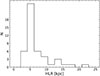 |
Fig. 7. Distribution of the sizes (in terms of HLR) of the Mg II halos. The halos were corrected by self-absorption before measuring their HLR using the absorption component of the best-fitting model. The radial profiles of the absorption-corrected Mg II emission halos are shown with a dashed line in Fig. 4. The HLR of each galaxy is provided in Table D.1. |
5. Fitting results
5.1. Best-fitting models
In Secs. 3 and 4, we have used the model only to correct for the self absorption in the observed spectra and infer the intrinsic surface brightness profile and size of the Mg II halos. For this correction, it is only relevant how well the spectral profile of the absorption line is modeled. However, we can also model the full Mg II absorption plus emission across a larger aperture to infer physical properties of galactic winds.
In this section, we provide an overview of the performance of our outflow model at reproducing the MUSE observations of the Mg II halos, as well as the overall distribution of the best-fitting parameters. The model has been introduced in Pessa et al. (2024), and we refer the reader to that paper for a complete description of our modeling scheme, its limitations, and main assumptions. In Appendix E.1, we include a summarized description of the model used, as well as our fitting approach.
In a few words, the outflow was modeled as an ensemble of spherical shells, where the velocity of each shell increases with radius such that continuum photons produced by the central source interact with the outflowing material only at the specific radius where the absorbing Mg II ions are at resonance (due to their Doppler shift), an assumption commonly known as the “Sobolev” approximation. The gas density (and thus optical depth) also varies radially, following the velocity field (assuming mass conservation).
The main free parameters that describe the wind properties are the launching velocity of the wind (v0), the launching radius of the wind (R0), its central optical depth (τ0), radial acceleration rate (γ), and terminal velocity (vmax). The biconical geometry is described through three additional parameters: the opening angle (O.A.) of the bicone, a rotation angle (R.A.) that measures the rotation of the outflow perpendicular to the plane of the sky toward the observer, and a position angle (P.A.) that corresponds to the angle of the outflow with respect to the horizontal axis in the plane of the sky. Lastly, an additional contribution of nebular emission to the Mg II is described by the fC parameter.
5.2. Comparison of data and best-fitting models
Figure 8 shows a detailed comparison between the MUSE data and the best-fitting models, in terms of the continuum-subtracted Mg II pseudo-narrowband images and the spectra extracted from annular apertures, for a galaxy drawn from one of the MUSCATEL fields. The continuum-subtracted pseudo-narrowband image exhibits a highly irregular morphology that the model cannot faithfully reproduce. However, when comparing the spectra extracted from azimuthally integrated apertures, it is clear that there is broad agreement between the data and the model, and that the line profiles of the Mg II absorption and emission are well captured by the outflow model. The inner apertures show a clear P-Cygni profile with a prominent absorption, and some emission that becomes progressively more dominant toward the outer apertures.
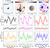 |
Fig. 8. Summary of the comparison of the observed and best-fitting model Mg II spectral profile and continuum-subtracted pseudo-narrowband images for an example galaxy in our final sample (M0416-SF7-012). The top-left panel shows the cutout of the HST F814W image around the galaxy, of 7 arcsec2 size. The top-middle panels show the observed (middle-left) and best-fitting model (middle-right) continuum-subtracted Mg II pseudo-narrowband images. The pseudo-narrowband images were created by collapsing the cubes across the wavelength axis, for wavelengths that enclose the full P-Cygni profile of the Mg II doublet. The size of the pseudo-narrowband images is the same as that of the HST F814W cutout. The two panels show net Mg II emission in black and net Mg II absorption in red. The residuals between both images are shown in the top-right panel. The rest of the panels show the integrated Mg II spectra on different annular (and circular) apertures for the data (solid) and best-fitting model (dashed) cubes. The residuals are shown in the small panels below, in units of standard deviations. The vertical dotted brown lines indicate the rest-frame wavelength of the Mg II doublet. The blue circle in the top-left panel shows the size of the full modeled region, and the black spectrum corresponds to the spectrum integrated over it. The rest of the panels that show colored spectra (and residuals) correspond to the comparison of the spectra extracted from the data and model cubes, in different annular and circular (in the case of the magenta spectra) apertures. In the legend of each panel, the inner and outer radii of the annular apertures are indicated. The color of the spectra in each panel matches the color of the circle in the top-left panel, which corresponds to the outer radii of its annular (or circular) aperture. The nearly horizontal dotted lines in each panel indicate the approximate continuum level. |
While we show here only an illustrative representative case from our sample, we include the modeling results for all our sample galaxies in Appendix B. Additionally, in Sec. 6.4, we discuss a subset of particular objects whose observed properties could indicate that their Mg II emission is not entirely described by our simple outflow model.
5.3. Distribution of best-fitting model parameters
In Sec. 5.1, we show some examples of the best-fitting model obtained for a subset of our sample galaxies. By fitting our outflow model to our entire sample, we can obtain, for the first time, a population-level distribution of galactic wind properties derived from the Mg II emission halos, moving forward from reporting the discovery and modeling of individual objects. Figure 9 shows the distribution of the best-fitting model parameters derived for our sample galaxies. The best-fitting parameters obtained for each individual galaxy, and their corresponding uncertainties, are provided in Table D.2.
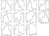 |
Fig. 9. Distribution of the best-fitting model parameters for our sample galaxies. The parameters of the model are described in detail in Appendix E.1. For R.A., we only included galaxies with non-isotropic outflows (O.A. < 75°), and for P.A., we considered only galaxies with non-isotropic outflows (O.A. < 75°) that are also not seen nearly face on (R.A. < 75°). The median and standard deviation of each distribution are indicated in each corresponding panel. The best-fitting parameters and their uncertainties obtained for each galaxy are provided in Table D.2. |
The distribution of central optical depth τ0 is centered around high values of 2.5 ≲ log τ0 ≲ 3.0, meaning that our model predicts a completely optically thick medium in the inner shells of the CGM. We find a median and standard deviation of log τ0 = 2.6 ± 0.6. We can also use Eq. E.6, together with the best-fitting values of r0 and v0 to infer the distribution of central Mg II number density n0,Mg II, obtaining a median and standard deviation values of log nn0,Mg II = − 6.3 ± 0.7 cm−3. This number is lower than the value derived for the galaxy UDF884 in Pessa et al. (2024) of −5.2 ± 0.2 cm−3, although consistent within less than two standard deviations. However, translating this value into a gas density is not straightforward since it would require knowledge about the underlying gas metallicity, ionization correction, and level of dust depletion of the Mg II ions.
The distribution of the index of the velocity power law γ exhibits median and standard deviation values of 1.0 ± 0.5, being generally lower than two. The fact that most galaxies show γ ∼ 1 suggests a linear relation between radius and velocity, and as a consequence, a density that falls as n ∝ r−3. However, a wind velocity that increases with radius does not unambiguously imply an accelerating wind. If there is a distribution of velocities for the gas leaving the ISM, gas with higher velocities tend to dominate at larger distances, even if the wind is not accelerating or decelerating at all radii (see also hydrodynamical simulations of SNe powered outflows from Dalla Vecchia & Schaye 2008). We caution the reader about this possible degeneracy in order to avoid an overinterpretation of our modeling results.
A density that decreases as n ∝ r−3 represents a steeper decrease with radius than that estimated from absorption line studies, which find a slope closer to n ∝ r−2 (Bouché et al., in prep.). While this result, taken at face value, might seem like a discrepancy, it can be explained by the fact that here we are only accounting for the currently outflowing gas that dominates the inner CGM. Additional gas in the CGM that is not outflowing, or that is connected to past outflow events, would not contribute to the inferred density profile. Thus, it is not unexpected that the density profile inferred from absorption line studies that account for all the absorbing gas present at some impact parameter from the central galaxy (regardless of their origin) is flatter than the one derived here. This additional contribution of non-outflowing gas would produce a profile that decreases more slowly than the one accounting for outflowing gas only.
The launching velocity of the winds is more widely distributed, with a median and standard deviation value of 62 ± 32 km s−1. This velocity increases radially up to maximum velocities of vmax = 490 ± 95 km s−1. These results are consistent with predictions from three-dimensional hydrodynamic simulations of supernovae-driven galactic winds (see, e.g., Fielding et al. 2017).
A maximum velocity of ∼490 km s−1 is significantly higher than the outflow velocities derived from absorption line studies (see, e.g., Schroetter et al. 2016, 2019, 2024; Bouché et al. 2025). Bouché et al. (2025) report outflow velocities that are generally closer to ∼200 km s−1, even in sight lines at impact parameters comparable with the size of the modeled regions in this work. However, despite this apparent disagreement, one must consider the nature of each measurement. While here, we infer the maximum radial velocity of the gas; absorption-line studies measure the line-of-sight projected velocity, averaged along a sight line at a specific impact parameter. This measurement has to be lower than our inferred maximum velocity, on one hand, because it only accounts for the component of the velocity parallel to the line of sight and, on the other, because it is an average (weighted by column density) along the line of sight, instead of strictly a maximum value.
The velocity offset Δv is distributed around relatively small offsets, with a median and standard deviation value of 56 ± 112 km s−1. This offset is shown, for instance, in the innermost apertures of Fig. C.3, where the rest-frame velocity of the Mg II doublet coincides with the absorption component of the P-Cygni profile, rather than with the peak of the emission. This offset could be explained either by the simplicity of the outflow model kinematics not being able to capture the actual kinematics of the galactic winds, as well as by an inaccurate redshift measurement that has been computed via a (supervised) template matching, rather than by modeling the continuum and/or emission lines of the spectra. In that line, we estimate that the accuracy of the redshift determination should be generally within ∼50 km s−1.
The additional nebular emission contribution, parametrized by the parameter log fC, presents a mildly bimodal distribution, where some galaxies essentially do not present any significant level of nebular emission (low fC). However, in most of them, some nebular emission is required to reproduce the observations.
Regarding the geometry of the outflows, we find mostly outflows with wide opening angles, with a median opening angle of 68° ±17°. These wide opening angles are, at least in part, a selection effect. Since by construction, our sample is composed of galaxies that exhibit both Mg II emission and absorption, and a wide opening angle makes it more likely to produce this spectral feature.
For the rotation angle in the direction of the sight line R.A., we find predominantly outflows pointing toward the observer, with a median and standard deviation of 51° ±18° (R.A. = 90° represents a face-on outflow). We only consider those outflows with an O.A. < 75°, since in the isotropic cases, where O.A. ∼90°, the definition of R.A. is meaningless. Similarly to the O.A., this is also, at least partially, a selection effect, since outflows pointing toward the observer are more likely to exhibit a P-Cygni profile and, thus, be a part of our sample. Outflows that lie nearly perpendicular to the line of sight would only be able to produce an absorption if they also have a very broad opening angle. Otherwise, they would be seen only in emissions.
For the distribution of the position angle in the plane of the sky, P.A., we consider only those cases that are not isotropic (O.A. < 75°) and that are not essentially face-on outflows (R.A. < 75°), because in both of these cases, the P.A. is essentially a physically meaningless quantity. For the remaining galaxies, although our statistics are low, we find a distribution without a strongly preferred orientation, consistent with what one would expect from the intrinsically random orientation of the outflow in the plane of the sky.
For the launching radii of the wind, as discussed in Appendix E.2.2, we use as prior the effective radius of each galaxy, measured with GALFIT, so it is not an entirely independent measured quantity. Nevertheless, the r0 values measured are consistent with the expected sizes of star-forming galaxies at 1.0 ≲ z ≲ 2.0 for the stellar mass range of our sample (see, e.g., van der Wel et al. 2014; Mowla et al. 2019; Nedkova et al. 2021). Finally, the parameter f, which scales the additional variance contribution, is generally small, with values mainly in the range log f < −2.5, indicating that a significant additional variance is not required to model our data.
We note that while the MUSE data cubes are extremely information-rich, some covariance between model parameters in the posterior distribution is present. These parameter covariances are discussed in greater detail in Pessa et al. (2024). For instance, we find a negative covariance between γ and v0, indicating that winds launched with higher initial velocities require a smaller radial increase in velocity to reproduce the data. Similarly, Δv shows covariance with both γ and v0, since the velocity offset is closely linked to the adopted velocity law. Along the same lines, because the optical depth gradient is directly related to the velocity gradient through the assumption of mass conservation, τ0 exhibits covariance with the parameters that govern the velocity (and hence optical-depth) gradient, namely γ and v0.
Nevertheless, while moderate parameter covariances are present, the model parameters do not exhibit strong degeneracies, in the sense that the model remains identifiable and distinct parameter combinations do not lead to statistically indistinguishable solutions. A multi-modality in the posterior distribution of the model parameters could also point to a degeneracy between the parameters, however, we do not observe this behavior in the obtained posterior distributions. Accordingly, the posterior distributions generally display well-defined modes, indicating that the parameters are well constrained, with the widths of the posterior distributions quantifying the associated uncertainties.
6. Discussion
6.1. Prevalence of cool-gas outflows traced by their extended Mg II emission
In Sec. 3.3.2 we show that, relative to our parent sample, galaxies in our final sample have higher SFR, higher sSFR, and younger age bins (see Fig. 6). While this appears to be an intuitive result, from the perspective of stellar-feedback driven outflows, there is no clear consensus in the literature on how the presence of galactic outflows depends on the galaxy properties.
Our results contrast with those of Rubin et al. (2014), who find a much higher fraction of galaxies with cool-gas outflows (66 ± 5%), traced by the presence of Mg II absorption in integrated spectra of 105 star-forming galaxies. In their study, the outflow detection rate primarily depends on galaxy inclination (with higher fractions in face-on galaxies) and shows little dependence on intrinsic galaxy properties. This difference could be due to the fact that we focus on outflows traced by extended emission rather than absorption. Outflows detected in Mg II absorption may trace different (and more common) gas structures than those that produce extended emission halos. The latter may require the outflowing material to escape to circumgalactic scales, rather than simply being launched, potentially linking extended emission to higher SFR, sSFR, and younger stellar populations. In support of this, Rubin et al. (2014) also report that the inferred strength and velocity of cool-gas outflows are correlated with host galaxy properties, which aligns with our findings.
Additionally, the stellar mass and SFR range of the Rubin et al. (2014) sample overlaps mainly with the high end of our distribution (log M* > 9.8 M⊙ and log SFR ≳ 0 M⊙ yr−1). When we include galaxies in our sample that show Mg II only in absorption and restrict our analysis to the same stellar mass and star formation ranges as Rubin et al. (2014), we find that any dependence on intrinsic galaxy properties largely disappears.
In a more recent work, Das et al. (2025) search for galaxies associated with intervening Mg II absorbers over a redshift range of 0.4 < z < 1.0. By identifying ∼270 Mg II–galaxy systems, they find that only a small fraction (∼10%) are associated with suppressed star formation (log(sSFR) < − 10.6 yr−1), implying a strong dependence of Mg II absorption on intrinsic galaxy properties, consistent with our results. This is further supported by several studies that find stronger cool-gas absorbers associated with star-forming galaxies than with passive ones (e.g., Bordoloi et al. 2014; Harvey et al. 2025).
In this line, Schroetter et al. (2024) use data from the MusE GAs FLOw and Wind survey (MEGAFLOW, Schroetter et al. 2016; Bouché et al. 2025) to explore correlations between the inferred galactic outflow properties probed by background quasars and host galaxy properties, and find that the velocity of the outflows is correlated with the host galaxy SFR and SFR surface density. Furthermore, they report a distinction between strong and weak outflows, based on the wind momentum compared to the momentum injection rate from SFR (following the formalism from Heckman et al. 2000), where strong outflows show a tighter correlation with galaxy properties.
Lastly, as detailed in Sec. 3.3.2, the fraction of galaxies with galactic-scale outflows in our sample not only depends on galaxy properties, but also on the depth of the data, varying significantly between the deep and shallow levels of MUSCATEL, especially for the highest SFR galaxies. In Appendix F we show the prevalence of galactic-scale outflows traced by Mg II for the different depth levels of the MUSCATEL survey (i.e., SF, MF, and DF). Figure F.1 shows that the prevalence of outflows for high-SFR galaxies is significantly higher for galaxies drawn from the DF and MF, compared to the SF. This implies that galactic outflows are probably a much more common feature among high-SFR galaxies than what Fig. 6 could initially suggest.
Overall, our findings are broadly consistent with previous work. However, it is important to keep in mind that galaxy populations exhibiting outflows traced in CGM emission and absorption may not be directly comparable, particularly when different stellar mass or SFR ranges are involved.
6.2. Correlation between host galaxy properties and outflow parameters
In this section, we show how the parameters of our best-fitting outflow model for each galaxy correlate with the host galaxy properties, specifically, their stellar mass, SFR, specific SFR, and SFR surface density. Figure 10 shows the derived outflow parameters as a function of the stellar mass of each galaxy. Overall, there are no clear correlations with stellar mass in our sample, meaning that the mechanisms that set the outflow properties are likely too complex to be described by a single quantity.
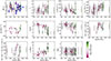 |
Fig. 10. Correlation of the best-fitting model parameters obtained with our outflow modeling scheme (see Appendix E.1) with the stellar mass of each galaxy, derived via SED fitting (see Sec. 2.2). The plots are color coded by the size of the Mg II halo of each galaxy, reported in Sec. 4, with green colors indicating halos in the extended regime of the distribution, and pink colors indicating more compact halos. The blue squares in the top-left panel indicate galaxies with a more robustly constrained τ0. For R.A., we only included galaxies with non-isotropic outflows (O.A. < 75°), and for P.A., we only considered galaxies with non-isotropic outflows (O.A. < 75°) that are also not seen nearly face on (R.A. < 75°). |
However, there are some tentative trends between stellar mass and certain model parameters. For instance, more massive galaxies seem to more frequently (although not exclusively) show higher acceleration rates (γ), and their outflows reach, in general, higher maximum velocities. The Pearson correlation coefficient ρ for this trend between vmax and stellar mass is 0.43, generally interpreted as a weak to moderate correlation. A correlation between outflow velocity and stellar mass is also consistent with the results from Rubin et al. (2014), where the authors find a similar dependency, inferring the outflow velocity from the Mg II absorption line profile in the integrated spectra of galaxies.
The nebular emission contribution appears to correlate with halo size (ρ ≈ −0.66), rather than with galaxy stellar mass, as more compact halos generally exhibit a higher nebular emission contribution (although galaxies with stronger nebular emission contributions seem to be predominantly low-mass galaxies). Nebular emission is, by construction, concentrated in the central region, following the continuum emission. Thus, it is a self-consistent result that galaxies with relatively stronger nebular emission (higher fC) also tend to be more compact.
Regarding the geometry of the outflows, we find that while less massive galaxies exhibit primarily isotropic outflows, more massive galaxies show a wider variety, with both low and high opening angles. In principle, this could be explained as the outflowing material escaping more easily through the ISM of less massive galaxies, compared to the most massive ones. Interestingly, A similar trend was reported by Nelson et al. (2021) for simulated Mg II halos, where the authors find axis ratios around one (i.e., nearly isotropic emission) for low-mass galaxies, and increasing values, with higher scatter for the more massive ones.
Finally, the central optical depth τ0 does not show a priori any sign of correlation with the host galaxy properties investigated here. However, we note that for several of our sample galaxies, τ0 is poorly constrained, and this is reflected in the error bars shown in the corresponding panel of Fig. 10. To explore whether these poorly constrained measurements could be hindering the identification of a trend, we have split our sample according to the uncertainty in their derived τ0. Those galaxies with a τ0 uncertainty lower than the median τ0 uncertainty of the full sample (∼0.6 dex) represent the subset of galaxies (half of the sample) with a better constrained τ0, and are marked with blue squares in the corresponding panels of Fig. 10. If we restrict our analysis to these galaxies, we then identify a tentative trend between stellar mass and τ0, where more massive galaxies appear to exhibit higher central optical depths (ρ = 0.39, interpreted as a moderate correlation).
A higher optical depth in more massive galaxies could be, at face value, interpreted as more massive galaxies having a more massive and denser CGM. However, there are additional relevant factors that would play a significant role in the relation between τ0 and the actual density of the outflow. The metallicity, dust depletion, and ionization correction will have a direct impact on the Mg II optical depth, at a given gas density (see, e.g., Martin et al. 2013). Furthermore, these mechanisms are also likely correlated with stellar mass, for instance, through the mass versus gas-phase metallicity correlation (Tremonti et al. 2004). Thus, a higher optical depth in a more massive galaxy could also be qualitatively explained by a higher metallicity, leading to a higher relative number of Mg II ions at a given gas density.
Nevertheless, keeping only those galaxies with a relatively more robust constraint on τ0 comes with the clear caveat of dropping mostly galaxies on the low-mass end of the distribution. It could be the case that either the higher uncertainty of τ0 in low-mass galaxies hinders the identification of a trend between stellar mass and central optical depth in the full sample, or that due to some astrophysical mechanism related, for instance, to the interplay between the strength of galactic winds and the gravitational potential of galaxies, low-mass galaxies do not follow the same trend as higher-mass galaxies. Unfortunately, with our current data and analyses, we cannot exclude any of those scenarios.
None of the other model parameters show a trend with galaxy stellar mass, except for r0, but this parameter is, by construction, tied to the continuum size of each galaxy. Therefore, a correlation between r0 and stellar mass is not unexpected.
Figure 11 shows the correlations of the outflow parameters with the sSFR of our sample galaxies. The trends with sSFR do not show any clear correlation. For SFR (not shown here), we observe trends similar to those seen with stellar mass, albeit with higher scatter.
The SFR surface density (ΣSFR) is also a relevant quantity in the context of SF-driven outflows. Heckman et al. (2015) find that the velocity of outflows measured from absorption lines in a sample of starburst galaxies correlates with ΣSFR. In the same line, Verhamme et al. (2017) find that high ΣSFR values promote low-density channels that facilitate the escape of Lyman continuum photons. Thus, we also explore possible correlations between the outflow properties and ΣSFR, using SFR/πHLRcont2 as a tracer of ΣSFR. Figure 12 shows these trends. However, there are no clear correlations. Perhaps similar trends to those observed with stellar mass, although with a higher scatter (similar to that observed with SFR). An intriguing aspect is that we find a broad range of ΣSFR for our sample galaxies, between log ΣSFR ∼ −4 and log ΣSFR ∼ 1. Some previous works have suggested minimum ΣSFR values required to launch strong galactic-scale outflows on the order of log ΣSFR ∼ −1 (Heckman et al. 2015) and log ΣSFR ∼ −2 (Reichardt Chu et al. 2025). On the other hand, while most (∼83%) of our sample galaxies exhibit log ΣSFR ≳ −2, this is not strictly always the case. Naturally, this comparison comes with the caveat that the ΣSFR of each galaxy is calculated globally, which does not rule out that locally, around the outflowing star-forming regions, ΣSFR could reach significantly higher values. Local physical conditions (e.g., ISM density, ΣSFR) are likely a key driver of star-forming driven outflows, besides global galactic properties.
In principle, it would be expected that the outflow properties correlate more closely with SFR, sSFR, and ΣSFR) than with stellar mass, since these quantities are more directly related to the amount of energy injected into the ISM by stellar feedback, powering the outflows. Furthermore, in Sec. 3.3.2, we show that our sample galaxies tend to be preferentially at higher SFR and sSFR values, compared to our parent sample. Nevertheless, several possibilities exist that could explain this higher scatter. First of all, the large systematic uncertainties in the SFR determination that arise, for instance, from the assumption on the shape of the SFH of galaxies (see, e.g., Wang et al. 2024). And while our SFR estimates are generally consistent with our independent measurement from the [O II] emission line, the latter is also subject to relevant systematic uncertainties, as it is a single-line-based measurement, such as non-star-formation ionization or dust reddening.
Finally, given the kinematics of the gas predicted by our modeling scheme, the timescales involved in the traveling of the outflowing gas from the launching radius into the observed Mg II halos are of the order of hundreds of megayears (Pessa et al. 2024). This means that the present-day SFR of a galaxy might not be directly correlated with the outflow properties that we see today. Instead, they would be more closely connected to past episodes of star formation. However, past bursts of SFR would not be properly quantified either by the SFR measured from the SED fitting (which assumes an underlying smooth SFH) or by the [O II] based SFR measurement (which probes SFR in much shorter timescales of < 10 Myr). In this line, in a recent work, Harvey et al. (2025) stack the Mg II absorption lines in the spectra of background quasars for a sample of quiescent, star-forming, and post-starburst galaxies, and find that post-starburst galaxies exhibit significantly stronger Mg II absorption within 1 Mpc than star-forming or quiescent galaxies of the same stellar mass. In a future paper, we aim to link the outflow properties to the recent SFH of galaxies, exploring if it is possible to connect features of the Mg II halos with a specific star formation event.
6.3. Drivers of the size of the Mg II halos
In Sec. 4, we described how the size of the Mg II halos is measured and shown the distribution of their HLRs. In this section, we search for correlations between these sizes and properties of the host galaxies.
The left panel of Fig. 13 presents the HLRs of the Mg II emission halos as a function of each galaxy’s stellar mass. While there is not any clear correlation between the HLRs and stellar masses (also not with SFRs, not shown here), it could be the case that the size of the more compact Mg II halos (HLR < 8 kpc) correlates with the stellar mass of the host galaxy (see inset in left panel of Fig. 13). Indeed, the Pearson correlation coefficient between HLR and stellar mass, for galaxies with HLRs smaller than 8 kpc is ρ ≈ 0.62, interpreted as a significant correlation.
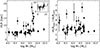 |
Fig. 13. Size of the Mg II emission halos after correcting by self-absorption as described in Sec. 4. The left panel shows the sizes of the Mg II emission halos as a function of the stellar mass of each galaxy, derived via SED fitting. The inset in the left panel shows a zoom-in to the HLR versus stellar mass relation for only those galaxies with HLR < 8 kpc. The right panel shows the ratio between the size of the Mg II emission halos and the size of the stellar component, as a function of the stellar mass of our sample galaxies. The horizontal dashed gray line shows the ratio of one for reference. |
This could potentially point out that while the Mg II emission closer to the galaxy is likely driven by mechanisms that correlate with stellar mass (e.g., outflows), the Mg II emission of more extended halos could also be powered by additional mechanisms, such as inflows, or the presence of satellites, that do not correlate directly with stellar mass. This would be consistent with our findings from Pessa et al. (2024), where we find larger differences between the observed Mg II emission and the prediction from our outflow-only model toward larger galactocentric distances for a galaxy in the MHUDF mosaic, potentially indicating the presence of additional mechanisms shaping the CGM of galaxies at larger spatial scales.
Furthermore, some of the galaxies with the most extended halos are actually not isolated systems. The objects AS1063-MF3-004 and AS1063-MF3-091 exhibit large (HLR > 10 kpc) Mg II halos, and they are a likely gravitationally interacting system (see discussion in Sec. C.1). The object AS1063-MF3-009 also presents an extended halo, and a relatively nearby galaxy (∼20 kpc in projected distance and a velocity offset of ∼1000 km s−1). In this case, the potential companion does not show a P-Cygni profile, and thus it is not part of our sample. The object A2744-SF1-062, for which we could not unambiguously determine a HST counterpart is also a possible ongoing merge, and exhibits a relatively large HLR of 8.6 kpc, although we cannot confirm this because the system is unresolved in the MUSE data, but it does present a disturbed morphology in the HST images.
This is probably not the only driver of the most extended halos, as the rest of the halos with HLR > 8 kpc do not show clear evidence of companion galaxies, given our detection limits. However, it does suggest that gravitational interaction between galaxies can be a relevant factor for setting the observed properties of the Mg II halos.
Nevertheless, the fact that we see mostly compact halos (HLR ≲5 kpc) for galaxies on the low-mass end of the stellar mass distribution could also be (at least partially) caused by a selection effect. As pointed out in Sec. 3, due to unavoidable selection effects, we could be missing the fainter and more extended halos, since they are intrinsically harder to detect.
We also explore trends between galaxy properties and the relative size of the halo with respect to the stellar counterpart. The right panel of Figure 13 shows the ratio between the halo size and the stellar size (i.e., continuum size) as a function of the stellar mass of our sample galaxies.
We find a wide range of values for this ratio, with halos being up to ∼7 times more extended than their stellar counterpart. However, we do not see any trend between the size ratio and stellar mass (nor for SFR, not shown here), implying that differences in size with respect to the stellar counterpart are not driven by mechanisms that correlate with stellar mass.
Leclercq et al. (2017) perform a similar measurement, for Lyα halos, also probing neutral gas halos, and find that the size of gaseous halos scales roughly linearly with the size of the stellar counterpart, being on average a factor 10 larger. In contrast, Fig. 13 shows that Mg II halos are on average a factor of about ∼2.5 larger than their stellar size (albeit with large scatter, and with several halos significantly more extended than this). It is not unexpected that halos traced by their Mg II emission are significantly smaller than those observed via their Lyα emission. Essentially, the lower optical depth of Mg II means that for a given density gradient, the CGM will become optically thin for Mg II earlier (at a lower galactocentric distance) than for Lyα photons, leading to more compact halos.
Lastly, for some galaxies the HLR of their Mg II emission is consistent with that of their stellar counterpart (i.e., a ratio of ∼1 in the right panel of Fig. 13). However, as detailed in Sec. 4, this does not necessarily mean that the Mg II emission distribution is consistent with that from the stellar counterpart. This is because the computation of the HLR involves azimuthally averaging the Mg II emission, whereas some halos show elongated shapes, and their outer areas would not significantly contribute to the azimuthally averaged profile. Furthermore, since by construction, we selected galaxies that exhibit central absorption of Mg II, this implies that the spatial distribution of the observed Mg II emission does not follow that of the continuum emission for any of our sample galaxies. For instance, for one of the most compact Mg II emitters in our sample (M0416-MF2-106, HLR ∼3.6 kpc), the corresponding panels of Fig. B.11 show that while the central apertures show both, Mg II absorption and emission, beyond  (yellow spectrum), there is essentially no continuum emission, but still clear Mg II emission. Thus, by construction, the spatial distribution of the Mg II emission will not be consistent with a scaled version of the stellar counterpart, for any of our sample galaxies, including the more compact ones.
6.4. Cases that potentially deviate from a simple outflow model
We find that the MUSE data from most of our sample galaxies can be well reproduced by a simple outflow model. However, the kinematics and morphology of the Mg II halos will always be more complex than the representation that the model provides, firstly, because outflows are not the only mechanisms at play in the CGM of galaxies and, secondly, because outflows themselves are much more complex than our implementation in terms of kinematics and small-scale structure, among other properties (see extended discussion about this in Pessa et al. 2024).
In Appendix C, we discuss in detail some particular cases that could potentially deviate from a simple outflow model. One of them is a seemingly gravitationally interacting system, where tidal forces could be actively shaping the properties of the Mg II emission halo. Another is a galaxy with a highly complex Mg II spectral profile, for which the outflow model performs poorly but may instead reflect a combination of inflow and outflow occurring simultaneously. Lastly, we discuss two galaxies whose Mg II emission toward large impact parameters is notoriously blueshifted with respect to the emission closer to the galaxy, and with respect to the expectations from our simple outflow scenario, pointing to the presence of more complex physics shaping the emission from their Mg II halo.
6.5. Outflow versus galaxy orientation
A relevant aspect of the model is the geometry and orientation of the outflow, parameterized by three angles (O.A., R.A., and P.A.; see Appendix E.1). In this section, we compare the outflow orientation inferred from the Mg II emission with that derived for the stellar counterpart of the same galaxies.
We use GALFIT to fit a 2D Sérsic model to the HST F814W image of each galaxy, which is dominated by stellar continuum emission, and measure their spatial orientation. Specifically, GALFIT provides the semi-axis ratio (q) and position angle of the Sérsic model.
From q, we calculated the inclination with respect to the line of sight as
 (2)
(2)
Here, I is the inclination of the galaxy in degrees such that for q = 1 (face-on disk), I = 90°, and for q ∼ 0 (edge-on disk), I ≈ 0°, consistent with the definition of R.A. in our model.
We compared the inclination inferred for each galaxy with its corresponding R.A. For perfectly polar outflows, the inclination should be roughly consistent with the R.A. We excluded nearly isotropic outflows (O.A. > 75°) as well as galaxies where q was too poorly constrained due to their irregular geometry.
Figure 14 shows R.A. as a function of the inclination inferred for the stellar counterpart. We did not find a systematic agreement between them, and we discuss several possible reasons for this. First of all, the formal uncertainties of the galaxy inclinations provided by GALFIT are small (< 1°) and are not shown in the figure. However, GALFIT orientations are subject to errors that are not captured by the formal uncertainties, for instance, due to irregular morphologies that are not consistent with a simple Sérsic model (even though the more extreme cases were excluded as mentioned above). For compact galaxies, estimating the inclination from the observed axis ratio is also uncertain. Lastly, since GALFIT essentially performs a light-weighted fit of the surface brightness, particularly bright star-forming regions can strongly bias the fit (e.g., a very bright star-forming center can lead to a rounder model, or a bright star-forming region in the disk of a face-on galaxy can produce an elongated geometry). Furthermore, it is not only that GALFIT can lead to biased results for the inclination. An actual inclination (and disk-plane or polar direction) could not even be well defined at all for some galaxies, as their definition relies on the assumption of an underlying disky geometry. And since we selected our sample based on the presence of large galactic-scale outflows, it might be the case that this feature also correlates with more disturbed morphological properties.
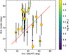 |
Fig. 14. Comparison of the orientation derived for the outflow (R.A.) with that inferred for the stellar disk of each galaxy from the HST F814W image using GALFIT. The dashed red line shows the identity, that is, when the inclination of the galaxy and the inclination of the outflow are the same. For a face-on polar outflow, both inclinations would be ∼90°, and for an edge-on polar outflow, both would be ∼0°. We have excluded from the figure galaxies that exhibit a nearly isotropic outflow (O.A. > 75°), as well as galaxies for which the inclination measured with GALFIT was too uncertain due to their complex surface brightness profile. The orange squares indicate galaxies with a measured continuum HLRs > 2 kpc. The formal uncertainties of the inclination provided by GALFIT are < 1°. |
With this caveat in mind, our results do not support a clear alignment between the Mg II outflow and the stellar disk. For nearly half of the galaxies, the direction of the outflow is not consistent with the inclination of the galaxy. This is also the case if we consider only galaxies with continuum HLRs larger than 2 kpc (indicated with orange squares in the figure).
While polar outflows are consistent with results from absorption line studies (e.g., Bouché et al. 2013) and simulations (e.g., Péroux et al. 2020), the small number of studies of Mg II halos in emission makes it difficult to unambiguously assess the orientation of outflows with respect to their host galaxies. For instance, Leclercq et al. (2022) find that the Mg II nebula in a group of five galaxies is well aligned with the semi-major axis of the most massive group member. On the other hand, Zabl et al. (2021) report a Mg II halo that is aligned with the semi-minor axis of its host galaxy, as would be expected from a polar outflow.
From stacking studies, Guo et al. (2023) find that edge-on galaxies present an excess of Mg II emission along their semi-minor axes, compared to their semi-major axes. However, comparing results from stacking with individual objects is not straightforward. We have selected the sample used in this work based on the presence of a P-Cygni profile in the Mg II line. In the context of polar outflows, this inevitably biases the sample toward more face-on orientations, excluding edge-on cases. Thus, our current sample, by construction, will lack the edge-on cases that produce the signature reported in Guo et al. (2023).
In that sense, the misalignment between galaxies and their outflows is also supported by the fact that we do not see a bias toward face-on orientations in the inclinations derived with GALFIT. Indeed, the highest inclination that we find among the sample (including those with nearly isotropic outflows, which are not shown in Fig. 14) is ∼64°. On the other hand, this expected bias toward face-on geometries is clearly seen in the distribution of the outflow R.A. This difference between the outflows and galaxies’ inclination distributions already suggests that these two quantities are not strictly connected. Furthermore, in another stacking study, Dutta et al. (2023) does not find a clear correlation between the surface brightness of Mg II halos and azimuthal angle, for a stack of ∼40 nearly edge-on galaxies.
A lack of correspondence between R.A. and galaxy inclination would suggest that the geometry of outflows is more complex than simply being ejected along the polar direction. In the context of star-forming driven outflows, this is not entirely unexpected. Star-forming regions are distributed across the galaxy disk, and they form stars in a stochastic manner. The ejection of ISM material by stellar feedback would thus naturally depend on the location of the star-forming region inside the disk, as well as the ISM conditions surrounding it (in addition to the energy input by the stellar feedback itself). And while generally, star-formation surface density (and thus feedback from star formation) is higher at the central regions of late-type galaxies (see, e.g., Ellison et al. 2021; Pessa et al. 2021), there is evidence that indicates that the radial mass assembly of low-mass galaxies (M* ≲ 9.3 M⊙) is more diverse, compared to more massive galaxies (Ibarra-Medel et al. 2016; Smith et al. 2022; Pessa et al. 2023). Moreover, in Guo et al. (2023), the authors find that for galaxies less massive than 9.5 M⊙, the differences between the edge-on and face-on stack samples essentially vanish.
Altogether, we find that the orientation of outflows with respect to their galaxy is not aligned with their semi-minor axis, suggesting that the interaction between the star-formation feedback and the surrounding ISM is complex and leads to a wider variety of geometries, rather than outflows being always ejected in the polar direction. However, a definitive assessment in this regard would require a more careful determination of the galaxy orientation, taking into account the stellar kinematics (which is beyond the scope of this paper), as well as accounting for differences between high- and low-mass galaxies.
7. Summary and conclusions
We have presented, for the first time, a population-level analysis of cool-gas galactic-scale outflows traced by their Mg II emission. To this end, we used deep MUSE data from the MUSCATEL survey and built a sample of 47 galaxies in which we detected significant Mg II extended emission and identified a P-Cygni spectral profile in the Mg II doublet, a characteristic signature of resonant scattering in an optically thick outflow.
Using this sample, we were able to study in a systematic manner the properties of their extended Mg II emission, such as morphology and spatial extent, and we used an outflow modeling scheme to infer the properties of the galactic winds powering the extended emission. Using available HST data, we were able to derive properties from the host galaxies and search for correlations between galactic wind properties derived from the extended Mg II emission and host-galaxy properties. Our main findings are the following:
-
Galaxies with extended Mg II emission tracing galactic-scale outflows are not necessarily significantly above the SFMS of galaxies or exclusively associated with starbursts. A fraction of them are significantly above the relation and could be cataloged as starbursting galaxies. However, most of them lie closer to (or even below) the SFMS.
-
Relative to our original parent sample, galaxies in our final sample are preferentially located in the high-end of the SFR and sSFR distributions, and they commonly show younger ages. However, even in the young and high SFR and sSFR regimes, the fraction of galaxies that present an outflow traced by their Mg II emission is low (∼20 − 30%). Altogether, this implies that having a certain SFR or a certain number of young stars does not strictly correlate with the presence of cool-gas outflows. Thus, there must also be other physical conditions required to produce a detectable outflow signal.
-
We corrected the Mg II emission for the self-absorption of the central galaxy, and we were able to derive the intrinsic size of the Mg II emission halos in terms of their HLR. We find that most of our sample galaxies exhibit halos with HLRs of ∼5 kpc, but the distribution also presents an extended tail of larger HLRs.
-
We do not identify any clear trend between the size of the Mg II emission halos and host-galaxy properties. However, we find a tentative correlation between the size of the halos on the compact side of the distribution (HLR ≲8 kpc) and the stellar mass of their host galaxy, potentially hinting at a difference in the mechanisms powering compact and extended halos.
-
Our outflow model is able to reproduce many of the features seen in the data in terms of spectral profile and general morphology. At the same time, residuals of the model also contain valuable information to put constraints on the physical mechanism shaping the CGM, such as additional secondary outflow components, or even hint at the presence of inflows.
-
We used our outflow modeling to derive the distribution of the galactic-wind properties, and we find that the inner regions of the wind are completely optically thick (log τ0 ∼ 2.6). The data are consistent with winds that accelerate nearly linearly with radius, from launching velocities of ∼60 km s−1 up to maximum velocities of ∼490 km s−1.
-
We investigated the correlations between the outflow properties and host galaxy properties, and we found tentative trends. More massive galaxies preferentially show higher maximum outflow velocities compared to less massive ones and perhaps also higher central optical depths than less massive ones. Regarding the geometry of the outflows, we find that low-mass galaxies show preferentially wider opening angles, while more massive galaxies show a much wider range of opening angles, which could be indicative of outflows escaping more easily through the ISM of less massive galaxies, compared to that of more massive ones.
-
Lastly, by comparing the inclination of our sample galaxies with those derived for the outflows, we find that the direction of the outflows is not strictly perpendicular to the disk plane, which could be due to the non-homogeneous distribution of SF regions across the galactic disk and the interaction between stellar feedback and the ISM. However, a more rigorous determination of the galaxy orientations with respect to the line of sight is needed to make a more robust claim in this regard.
These findings represent a significant step forward in understanding the occurrence and nature of cool-gas galactic outflows traced by Mg II emission. By combining deep integral-field spectroscopy with detailed outflow modeling and host-galaxy characterization, we have highlighted both the diversity and the complexity of mechanisms driving these winds. The presence of outflows in galaxies that are not strongly offset from the SFMS, the moderate detection fraction even among high-sSFR systems, and the tentative correlations with stellar mass all point to a multifaceted interplay between internal galaxy properties and the conditions necessary to launch and sustain cool-gas outflows. Future studies expanding the sample size, incorporating multiwavelength constraints, using more sophisticated modeling (e.g., radiative transfer simulations), and taking into account the recent star-formation history of galaxies will be crucial to fully disentangling the physical processes at play and to place these outflows in the broader context of galaxy evolution and baryon cycling in the CGM.
Acknowledgments
We thank the referee for their insightful and constructive comments, which have improved the paper. This project has received funding from the European Research Council (ERC) under the European Union’s Horizon 2020 research and innovation programme (grant agreement 101020943, SPECMAP-CGM). LW acknowledges funding by the Deutsche Forschungsgemeinschaft, Grant Wi 1369/32-1. JP and LW acknowledge funding by the Deutsche Forschungsgemeinschaft, Grant Wi 1369/31-1. We thank contributors to SCIPY (Virtanen et al. 2020), MATPLOTLIB (Hunter 2007), NUMPY (Harris et al. 2020), ASTROPY (Astropy Collaboration 2013, 2018), and the PYTHON programming language; the free and open-source community; and the NASA Astrophysics Data System for software and services. We also thank contributors to linetools (Prochaska et al. 2016) and PyMUSE (Pessa & Tejos 2020).
References
- Ambartsumian, V. A. 1958, Theoretical Astrophysics (New York: Pergamon Press) [Google Scholar]
- Astropy Collaboration (Price-Whelan, A. M., et al.) 2018, AJ, 156, 123 [Google Scholar]
- Astropy Collaboration (Robitaille, T. P., et al.) 2013, A&A, 558, A33 [NASA ADS] [CrossRef] [EDP Sciences] [Google Scholar]
- Bacon, R., Accardo, M., Adjali, L., et al. 2010, SPIE, 773508 [Google Scholar]
- Bacon, R., Conseil, S., Mary, D., et al. 2017, A&A, 608, A1 [NASA ADS] [CrossRef] [EDP Sciences] [Google Scholar]
- Bacon, R., Brinchmann, J., Conseil, S., et al. 2023, A&A, 670, A4 [NASA ADS] [CrossRef] [EDP Sciences] [Google Scholar]
- Baldwin, J. A., Phillips, M. M., & Terlevich, R. 1981, PASP, 93, 5 [Google Scholar]
- Barbani, F., Pascale, R., Marinacci, F., et al. 2025, A&A, 697, A121 [NASA ADS] [CrossRef] [EDP Sciences] [Google Scholar]
- Bezanson, R., Labbe, I., Whitaker, K. E., et al. 2024, ApJ, 974, 92 [NASA ADS] [CrossRef] [Google Scholar]
- Bordoloi, R., Lilly, S. J., Hardmeier, E., et al. 2014, ApJ, 794, 130 [NASA ADS] [CrossRef] [Google Scholar]
- Bouché, N. F., Hohensee, W., Vargas, R., et al. 2012, MNRAS, 426, 801 [CrossRef] [Google Scholar]
- Bouché, N. F., Murphy, M. T., Kacprzak, G. G., et al. 2013, Science, 341, 50 [CrossRef] [Google Scholar]
- Bouché, N. F., Wendt, M., Zabl, J., et al. 2025, A&A, 694, A67 [NASA ADS] [CrossRef] [EDP Sciences] [Google Scholar]
- Brinchmann, J., Charlot, S., White, S. D. M., et al. 2004, MNRAS, 351, 1151 [Google Scholar]
- Bruzual, G., & Charlot, S. 2003, MNRAS, 344, 1000 [NASA ADS] [CrossRef] [Google Scholar]
- Burchett, J. N., Rubin, K. H. R., Prochaska, J. X., et al. 2021, ApJ, 909, 151 [NASA ADS] [CrossRef] [Google Scholar]
- Byrohl, C., & Gronke, M. 2020, A&A, 642, L16 [NASA ADS] [CrossRef] [EDP Sciences] [Google Scholar]
- Calzetti, D., Armus, L., Bohlin, R. C., et al. 2000, ApJ, 533, 682 [NASA ADS] [CrossRef] [Google Scholar]
- Carr, C., & Scarlata, C. 2022, ApJ, 939, 47 [Google Scholar]
- Castor, J. I. 1970, MNRAS, 149, 111 [NASA ADS] [Google Scholar]
- Castor, J. I., & Lamers, H. J. G. L. M. 1979, ApJS, 39, 481 [NASA ADS] [CrossRef] [Google Scholar]
- Chabrier, G. 2003, PASP, 115, 763 [Google Scholar]
- Chang, S.-J., & Gronke, M. 2024, MNRAS, 532, 3526 [NASA ADS] [CrossRef] [Google Scholar]
- Chang, S.-J., Dutta, R., Gronke, M., et al. 2025, MNRAS, 542, 525 [Google Scholar]
- Chisholm, J., Prochaska, J. X., Schaerer, D., Gazagnes, S., & Henry, A. 2020, MNRAS, 498, 2554 [CrossRef] [Google Scholar]
- Chung, A. S., Dijkstra, M., Ciardi, B., Kakiichi, K., & Naab, T. 2019, MNRAS, 484, 2420 [NASA ADS] [CrossRef] [Google Scholar]
- Daddi, E., Dickinson, M., Morrison, G., et al. 2007, ApJ, 670, 156 [NASA ADS] [CrossRef] [Google Scholar]
- Dalla Vecchia, C., & Schaye, J. 2008, MNRAS, 387, 1431 [Google Scholar]
- Das, S., Joshi, R., Chaudhary, R., et al. 2025, A&A, 695, A207 [NASA ADS] [CrossRef] [EDP Sciences] [Google Scholar]
- Dutta, R., Fossati, M., Fumagalli, M., et al. 2023, MNRAS, 522, 535 [NASA ADS] [CrossRef] [Google Scholar]
- Ellison, S. L., Lin, L., Thorp, M. D., et al. 2021, MNRAS, 501, 4777 [NASA ADS] [CrossRef] [Google Scholar]
- Emsellem, E., Schinnerer, E., Santoro, F., et al. 2022, A&A, 659, A191 [NASA ADS] [CrossRef] [EDP Sciences] [Google Scholar]
- Erb, D. K., Steidel, C. C., & Chen, Y. 2018, ApJ, 862, L10 [Google Scholar]
- Erb, D. K., Li, Z., Steidel, C. C., et al. 2023, ApJ, 953, 118 [NASA ADS] [CrossRef] [Google Scholar]
- Feltre, A., Bacon, R., Tresse, L., et al. 2018, A&A, 617, A62 [NASA ADS] [CrossRef] [EDP Sciences] [Google Scholar]
- Fernandez-Figueroa, A., Lopez, S., Tejos, N., et al. 2022, MNRAS, 517, 2214 [NASA ADS] [CrossRef] [Google Scholar]
- Fernández-Figueroa, A., Kacprzak, G. G., Barone, T. M., et al. 2025, MNRAS, 544, 255 [Google Scholar]
- Fielding, D., Quataert, E., Martizzi, D., & Faucher-Giguère, C.-A. 2017, MNRAS, 470, L39 [CrossRef] [Google Scholar]
- Finley, H., Bouché, N. F., Contini, T., et al. 2017a, A&A, 605, A118 [NASA ADS] [CrossRef] [EDP Sciences] [Google Scholar]
- Finley, H., Bouché, N. F., Contini, T., et al. 2017b, A&A, 608, A7 [NASA ADS] [CrossRef] [EDP Sciences] [Google Scholar]
- Foreman-Mackey, D., Hogg, D. W., Lang, D., & Goodman, J. 2013, PASP, 125, 306 [Google Scholar]
- Fossati, M., Fumagalli, M., Lofthouse, E. K., et al. 2019, MNRAS, 490, 1451 [NASA ADS] [CrossRef] [Google Scholar]
- Gelman, A., & Rubin, D. B. 1992, Stat. Sci., 7, 457 [Google Scholar]
- Grinin, V. P. 2001, Astrophysics, 44, 402 [NASA ADS] [CrossRef] [Google Scholar]
- Guo, Y., Bacon, R., Bouché, N. F., et al. 2023, Nature, 624, 53 [NASA ADS] [CrossRef] [Google Scholar]
- Guo, Y., Bacon, R., Wisotzki, L., et al. 2024, A&A, 691, A66 [NASA ADS] [CrossRef] [EDP Sciences] [Google Scholar]
- Harris, C. R., Millman, K. J., van der Walt, S. J., et al. 2020, Nature, 585, 357 [NASA ADS] [CrossRef] [Google Scholar]
- Harvey, Z., Krishna, S., Wild, V., Tojeiro, R., & Hewett, P. 2025, Open J. Astrophys., 8, 47836 [Google Scholar]
- Heckman, T. M., Lehnert, M. D., Strickland, D. K., & Armus, L. 2000, ApJS, 129, 493 [Google Scholar]
- Heckman, T. M., Alexandroff, R. M., Borthakur, S., Overzier, R., & Leitherer, C. 2015, ApJ, 809, 147 [Google Scholar]
- Hemmati, S., Mobasher, B., Darvish, B., et al. 2015, ApJ, 814, 46 [Google Scholar]
- Henry, A., Berg, D. A., Scarlata, C., Verhamme, A., & Erb, D. 2018, ApJ, 855, 96 [Google Scholar]
- Herenz, E. C., & Wisotzki, L. 2017, A&A, 602, A111 [NASA ADS] [CrossRef] [EDP Sciences] [Google Scholar]
- Hunter, J. D. 2007, Comput. Sci. Eng., 9, 90 [NASA ADS] [CrossRef] [Google Scholar]
- Ibarra-Medel, H. J., Sánchez, S. F., Avila-Reese, V., et al. 2016, MNRAS, 463, 2799 [NASA ADS] [CrossRef] [Google Scholar]
- Kacprzak, G. G., Oppenheimer, B., Nielsen, N., et al. 2025, PASA, 42 [Google Scholar]
- Kelleher, D. E., & Podobedova, L. I. 2008, J. Phys. Chem. Ref. Data, 37, 267 [NASA ADS] [CrossRef] [Google Scholar]
- Kewley, L. J., Geller, M. J., & Jansen, R. A. 2004, AJ, 127, 2002 [Google Scholar]
- Kriek, M., van Dokkum, P. G., Labbé, I., et al. 2009, ApJ, 700, 221 [Google Scholar]
- Kusakabe, H., Shimasaku, K., Momose, R., et al. 2019, PASJ, 71, 55 [NASA ADS] [CrossRef] [Google Scholar]
- Kusakabe, H., Verhamme, A., Blaizot, J., et al. 2022, A&A, 660, A44 [NASA ADS] [CrossRef] [EDP Sciences] [Google Scholar]
- Kusakabe, H., Mauerhofer, V., Verhamme, A., et al. 2024, A&A, 691, A255 [NASA ADS] [CrossRef] [EDP Sciences] [Google Scholar]
- Leclercq, F., Bacon, R., Wisotzki, L., et al. 2017, A&A, 608, A8 [NASA ADS] [CrossRef] [EDP Sciences] [Google Scholar]
- Leclercq, F., Verhamme, A., Epinat, B., et al. 2022, A&A, 663, A11 [NASA ADS] [CrossRef] [EDP Sciences] [Google Scholar]
- Leibundgut, B., Bacon, R., Jaffé, Y. L., et al. 2017, The Messenger, 170, 20 [NASA ADS] [Google Scholar]
- Martin, C. L., Shapley, A. E., Coil, A. L., et al. 2013, ApJ, 770, 41 [NASA ADS] [CrossRef] [Google Scholar]
- Mitchell, P. D., Blaizot, J., Cadiou, C., et al. 2021, MNRAS, 501, 5757 [Google Scholar]
- Mowla, L. A., van Dokkum, P., Brammer, G. B., et al. 2019, ApJ, 880, 57 [NASA ADS] [CrossRef] [Google Scholar]
- Nedkova, K. V., Häußler, B., Marchesini, D., et al. 2021, MNRAS, 506, 928 [NASA ADS] [CrossRef] [Google Scholar]
- Nelson, D., Pillepich, A., Springel, V., et al. 2019a, MNRAS, 490, 3234 [Google Scholar]
- Nelson, D., Springel, V., Pillepich, A., et al. 2019b, Comput. Astrophys. Cosmol., 6, 2 [Google Scholar]
- Nelson, D., Byrohl, C., Peroux, C., Rubin, K. H. R., & Burchett, J. N. 2021, MNRAS, 507, 4445 [NASA ADS] [CrossRef] [Google Scholar]
- Noeske, K. G., Weiner, B. J., Faber, S. M., et al. 2007, ApJ, 660, L43 [CrossRef] [Google Scholar]
- Pagul, A., Sánchez, F. J., Davidzon, I., & Mobasher, B. 2021, ApJS, 256, 27 [NASA ADS] [CrossRef] [Google Scholar]
- Peng, C. Y., Ho, L. C., Impey, C. D., & Rix, H.-W. 2002, AJ, 124, 266 [Google Scholar]
- Peng, C. Y., Ho, L. C., Impey, C. D., & Rix, H.-W. 2010, AJ, 139, 2097 [Google Scholar]
- Péroux, C., Nelson, D., van de Voort, F., et al. 2020, MNRAS, 499, 2462 [CrossRef] [Google Scholar]
- Pessa, I., Tejos, N., & Moya1, C., 2020, ASP Conf. Ser., 522, 61 [Google Scholar]
- Pessa, I., Schinnerer, E., Belfiore, F., et al. 2021, A&A, 650, A134 [NASA ADS] [CrossRef] [EDP Sciences] [Google Scholar]
- Pessa, I., Schinnerer, E., Sanchez-Blazquez, P., et al. 2023, A&A, 673, A147 [NASA ADS] [CrossRef] [EDP Sciences] [Google Scholar]
- Pessa, I., Wisotzki, L., Urrutia, T., et al. 2024, A&A, 691, A5 [NASA ADS] [CrossRef] [EDP Sciences] [Google Scholar]
- Pharo, J., Wisotzki, L., Urrutia, T., et al. 2024, A&A, 690, A343 [NASA ADS] [CrossRef] [EDP Sciences] [Google Scholar]
- Pillepich, A., Nelson, D., Springel, V., et al. 2019, MNRAS, 490, 3196 [Google Scholar]
- Popesso, P., Concas, A., Cresci, G., et al. 2023, MNRAS, 519, 1526 [Google Scholar]
- Prochaska, J. X., Kasen, D., & Rubin, K. 2011, ApJ, 734, 24 [Google Scholar]
- Prochaska, J. X., Tejos, N., Crighton, N., et al. 2016, https://doi.org/10.5281/zenodo.168270 [Google Scholar]
- Reichardt Chu, B., Fisher, D. B., Chisholm, J., et al. 2025, MNRAS, 536, 1799 [Google Scholar]
- Remolina-Gutiérrez, M. C., & Forero-Romero, J. E. 2019, MNRAS, 482, 4553 [Google Scholar]
- Reynaldi, V., & Feinstein, C. 2013, MNRAS, 435, 1350 [Google Scholar]
- Rihtaršič, G., Bradač, M., Desprez, G., et al. 2025, A&A, 696, A15 [NASA ADS] [CrossRef] [EDP Sciences] [Google Scholar]
- Rubin, K. H. R., Prochaska, J. X., Ménard, B., et al. 2011, ApJ, 728, 55 [NASA ADS] [CrossRef] [Google Scholar]
- Rubin, K. H. R., Prochaska, J. X., Koo, D. C., et al. 2014, ApJ, 794, 156 [Google Scholar]
- Schroetter, I., Bouché, N. F., Wendt, M., et al. 2016, ApJ, 833, 39 [NASA ADS] [CrossRef] [Google Scholar]
- Schroetter, I., Bouché, N. F., Zabl, J., et al. 2019, MNRAS, 490, 4368 [CrossRef] [Google Scholar]
- Schroetter, I., Bouché, N. F., Zabl, J., et al. 2024, A&A, 687, A39 [NASA ADS] [CrossRef] [EDP Sciences] [Google Scholar]
- Scuderi, S., Bonanno, G., di Benedetto, R., Spadaro, D., & Panagia, N. 1992, ApJ, 392, 201 [NASA ADS] [CrossRef] [Google Scholar]
- Shipley, H. V., Lange-Vagle, D., Marchesini, D., et al. 2018, ApJS, 235, 14 [Google Scholar]
- Smith, M. V., van Zee, L., Dale, D. A., et al. 2022, MNRAS, 515, 3270 [NASA ADS] [CrossRef] [Google Scholar]
- Sobolev, V. V. 1960, Moving Envelopes of Stars (Cambridge: Harvard University Press) [Google Scholar]
- Song, H., Seon, K.-I., & Hwang, H. S. 2020, ApJ, 901, 41 [NASA ADS] [CrossRef] [Google Scholar]
- Tremonti, C. A., Heckman, T. M., Kauffmann, G., et al. 2004, ApJ, 613, 898 [Google Scholar]
- Tumlinson, J., Peeples, M. S., & Werk, J. K. 2017, ARA&A, 55, 389 [Google Scholar]
- Turner, M. L., Schaye, J., Crain, R. A., et al. 2017, MNRAS, 471, 690 [NASA ADS] [CrossRef] [Google Scholar]
- Urrutia, T., Wisotzki, L., Kerutt, J., et al. 2019, A&A, 624, A141 [NASA ADS] [CrossRef] [EDP Sciences] [Google Scholar]
- van der Wel, A., Franx, M., van Dokkum, P. G., et al. 2014, ApJ, 788, 28 [Google Scholar]
- Verhamme, A., Orlitová, I., Schaerer, D., et al. 2017, A&A, 597, A13 [NASA ADS] [CrossRef] [EDP Sciences] [Google Scholar]
- Virtanen, P., Gommers, R., Oliphant, T. E., et al. 2020, Nature Methods, 17, 261 [CrossRef] [Google Scholar]
- Wang, B., Leja, J., Atek, H., et al. 2024, ApJ, 963, 74 [CrossRef] [Google Scholar]
- Weilbacher, P. M., Streicher, O., Urrutia, T., et al. 2014, ASP Conf. Ser., 485, 451 [NASA ADS] [Google Scholar]
- Weilbacher, P. M., Palsa, R., Streicher, O., et al. 2020, A&A, 641, A28 [NASA ADS] [CrossRef] [EDP Sciences] [Google Scholar]
- Werk, J. K., Prochaska, J. X., Tumlinson, J., et al. 2014, ApJ, 792, 8 [NASA ADS] [CrossRef] [Google Scholar]
- Wisotzki, L., Bacon, R., Blaizot, J., et al. 2016, A&A, 587, A98 [NASA ADS] [CrossRef] [EDP Sciences] [Google Scholar]
- Xu, X., Heckman, T., Henry, A., et al. 2022, ApJ, 933, 222 [NASA ADS] [CrossRef] [Google Scholar]
- Zabl, J., Bouché, N. F., Schroetter, I., et al. 2019, MNRAS, 485, 1961 [NASA ADS] [CrossRef] [Google Scholar]
- Zabl, J., Bouché, N. F., Schroetter, I., et al. 2020, MNRAS, 492, 4576 [NASA ADS] [CrossRef] [Google Scholar]
- Zabl, J., Bouché, N. F., Wisotzki, L., et al. 2021, MNRAS, 507, 4294 [NASA ADS] [CrossRef] [Google Scholar]
For A370, only one ‘deep field’ with a total exposure time of 10 hours was observed.
For the shallow fields, we used a S/N threshold of 6.
Median F814W mag of ∼23.4, with the faintest having a F814W mag of ∼25.5, significantly brighter than the detection threshold of the HFF HST data of ∼28 mag; see Shipley et al. (2018).
Appendix A: Compilation of continuum-subtracted Mg II pseudo-narrowband images and Mg II surface brightness radial profiles for the remaining galaxies in our sample
In this appendix, we present the continuation of Fig. 4, including the rest of our sample galaxies.
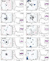 |
Fig. A.1. (Continued.) |
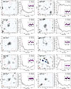 |
Fig. A.1. (Continued.) |
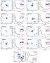 |
Fig. A.1. (Continued.) |
Appendix B: Model results for all our sample galaxies
Here we show the figures that compare the data and best-fitting model cubes, analogous to the figure shown in Sec. 5.1, for all our sample galaxies. Figures B.1, B.2, B.3, B.4, B.5, B.6, B.7, B.8, B.9, B.10, B.11, and B.12 summarize the modeling results for each galaxy in our sample. Galaxies are sorted by stellar mass, in descending order.
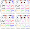 |
Fig. B.1. Comparison between the observed and best-fitting model cubes, in terms of the continuum-subtracted pseudo-narrowband images and spectra extracted from annular apertures for four sample galaxies. Each set of panels corresponds to one galaxy, following the same layout as in Fig. 8 (see caption of Fig. 8 for a full description of each panel). |
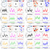 |
Fig. B.10. Same as Fig. B.1, but for four other galaxies in our sample. |
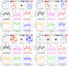 |
Fig. B.11. Same as Fig. B.1, but for four other galaxies in our sample. |
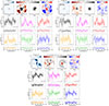 |
Fig. B.12. Same as Fig. B.1, but for three other galaxies in our sample. |
Appendix C: Discussion on particular cases
In this appendix, we discuss two particular cases that could potentially deviate from a simple outflow model, in a broader sense than exhibiting more complex Mg II velocity components within their Mg II halo.
C.1. A potentially interacting system
Two of our sample galaxies (AS1063-MF3-004 and AS1063-MF3-091) are actually physical neighbors, with a projected separation of ∼18 kpc, and a velocity difference of ∼160 km s−1. Figure C.1 shows the HST, continuum-subtracted Mg II pseudo-narrowband images, and the best-fitting model for these two galaxies.
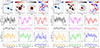 |
Fig. C.1. Comparison between data and model cube for two galaxies in our sample (AS1063-MF3-004 and AS1063-MF3-091) that are physical neighbors, with a projected separation of ∼18 kpc, and a velocity difference of ∼160 km s−1, whose Mg II halo could potentially be interacting and thus deviating from a simple outflow model. The set of panels on the left side of the figure shows the data and best-fitting model comparison for AS1063-MF3-004, and the right set of panels shows the same for AS1063-MF3-091. The layout of each set of panels is the same as in Fig. C.3, comparing the continuum-subtracted Mg II pseudo-narrowband images and the spectra extracted from annular apertures from the data and best-fitting model cube. The nearby galaxies have been masked during the fitting of each individual galaxy. |
The pseudo-narrowband images show that there is indeed a significant detection of Mg II emission surrounding both of these galaxies. This ‘shared’ Mg II halo is also seen in the corresponding panels of Fig. 4. We have modeled the Mg II halo of each galaxy independently, neglecting any additional contribution from the neighbor galaxy (the neighbor galaxy has been masked out during each fitting). This can potentially lead to the misrepresentation of the Mg II emission by the model seen in Fig. C.1, especially in the outer apertures. There is more Mg II emission in the outer apertures in the data cube, compared to the best-fitting model (especially for AS1063-MF3-004), and with seemingly more complex kinematics.
Another possibility is that the Mg II halo belongs to (in the sense that it is produced by) only one of the galaxies in the system. In that line, the kinematics of the Mg II emission are more consistent with the more massive galaxy of the pair AS1063-MF3-004 (offset with respect to systemic velocity Δv = 4 km s−1) than with the less massive one AS1063-MF3-091 (Δv = 120 km s−1). However, an offset of 120 km s−1 is not unusual in our sample, and it is consistent with the rest of the sample, composed of essentially isolated galaxies. On the other hand, the morphology of the halo does not suggest that the halo is produced by just one of the galaxies of the pair. If this were the case, it would imply an extremely asymmetric and elongated halo. One could speculate that the gravitational interaction could, in principle, produce such morphology, driving the outflowing gas toward the second galaxy. Nevertheless, there is not yet strong evidence that this is the case, and modeling both galaxies independently produces a reasonable output. While using a more sophisticated model is outside the scope of this paper, systems like this can provide observational evidence of how the physical properties of cool gas halos are affected by nearby galaxies, and how they can impact the baryon cycle.
C.2. Possible inflow signature
While there is evidence that suggests that cool accretion flows could become the dominant mechanisms shaping the CGM at large impact parameters (b ≳ 50 kpc; see, e.g., Turner et al. 2017; Chung et al. 2019), absorption line studies find that extended accretion disks aligned with the semi-major axis of galaxies can be present at smaller impact parameters (b ∼ 10 kpc Zabl et al. 2019). Fernández-Figueroa et al. (2025) also find evidence that suggests that ultra-strong Mg II absorbers in the sight lines of background quasi-stellar objects at b ≲ 30 kpc, and down the barrel, could be probing cool-gas inflows. This additional inflowing component could certainly leave an imprint in the Mg II emission halo that our outflow model might not be able to capture. In this line, one of our sample galaxies (A2744-DF-013) exhibits a morphology and Mg II spectral profile that seems to be incompatible with our outflow model.
The left section of Fig. C.2 shows the data and best-fitting model for this galaxy, using our fiducial outflow model. It is clear that the data present characteristics that are too complex for the model to reproduce. The inner apertures are dominated by a strong and broad absorption, with likely more than one absorbing kinematic component, and the outer apertures exhibit strong Mg II emission. In between, the spectral profile of the line becomes extremely complex, with even a seemingly inverted P-Cygni profile, which could be indicative of inflowing gas. Interestingly, the full aperture-integrated spectrum does not show any clear Mg II P-Cygni profile, and only the Mg II 2796 line shows up cleanly in emission. The high S/N of the data implies that this complex spectral profile is real, and not a noise-driven feature. Additionally, both the absorption and the emission features are well centered at the systemic velocity.
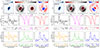 |
Fig. C.2. Comparison between data and model cube for one of our sample galaxies (A2744-DF-013) whose Mg II emission halo exhibits characteristics that are inconsistent with our purely outflow emission model. By including an additional inflow-absorbing contribution to the model, we are able to reproduce the data more closely. The parameterization of the inflow component is detailed in the main text (see Sec C.2). The set of panels on the left side of the figure shows the data and best-fitting model comparison for A2744-DF-013, using our fiducial outflow-only model described in Appendix E.1. The right set of panels shows the same for our outflow+inflow model. The layout of each set of panels is the same as in Fig. C.3, comparing the continuum-subtracted Mg II pseudo-narrowband images and the spectra extracted from annular apertures from the data and best-fitting model cube. |
While the model attempts to capture these features, it clearly lacks the complexity to reproduce the data. Specifically, the model suggests a nearly face-on outflow (R.A. = 71°) that would indeed exhibit only absorption at low impact parameters, and only emission at larger galactocentric distances. However, the predicted level of emission falls short with respect to the data in the outer apertures by a significant margin. The overall shape and velocity of the Mg II spectrum are also not well captured by the model.
In order to improve the model and provide a more accurate representation of the data, we have included an additional inflowing absorption contribution. The motivation is that inflowing gas absorbing light from the central galaxy in the innermost line of sights could produce a signal similar to what is seen in the data, such as strong absorption at nearly the same velocity as the Mg II emission, that could totally or partially cancel out in the integrated spectrum, as well as the inverted P-Cygni profile seen in the yellow aperture.
To parametrize the gas inflow, we have employed a similar formalism used for the outflowing gas, following the implementation from Carr & Scarlata (2022), where the velocity of the inflowing gas also varies radially as
 (C.1)
(C.1)
where v = v∞ − v0, in would represent the maximum velocity of the inflowing gas, reached at r = R0. The accretion begins from rest at r = Rmax, in, and then the gas is radially accelerated during its infall up to the maximum velocity, at a rate that depends on v0, in and γin. This simple scenario is consistent with gas that is ejected from the galaxy and eventually reaccreted (Barbani et al. 2025).
This different assumed velocity law implies that instead of solving Eq. E.3 to determine the bijective relation between observed velocity and radius, we had to instead solve
![Mathematical equation: $$ \begin{aligned} r^{2} - R_{0}^{2} \, \biggl (1 - \biggl [\frac{\epsilon }{r}\biggr ]^{2} \biggr )^{\frac{\gamma _{\mathrm{in}} - 1}{\gamma _{\mathrm{in}}}} \biggl (\frac{v_{\infty } (1 - \frac{\epsilon ^2}{r^2} )^{0.5} - v_{\mathrm{obs}}}{v_{0,\mathrm{in}}} \biggr )^{2/\gamma _{\mathrm{in}}} - \epsilon ^{2}= 0. \end{aligned} $$](/articles/aa/full_html/2026/04/aa57875-25/aa57875-25-eq15.gif) (C.2)
(C.2)
Finally, to compute the inflow optical depth τin at a given radius, we use the same Eq. E.7 as for the outflow, but using a different parameter τ0, in to describe the optical depth at r = R0 for the inflowing gas, and γin for the acceleration rate. A total of four additional parameters are required to add this additional contribution into the model (v∞, v0, in, γin, and τ0, in).
In Carr & Scarlata (2022), the authors show that using this parametrization, the isovelocity curves (i.e., surfaces of constant observed velocity; see also Appendix E.1) bend back into the central source, meaning that for impact parameters larger than the source size R0, any given sight line will intersect the same isovelocity curve more than once (as opposed from the outflow case, where the isovelocity curves do not bend, and are intersected always only once by any given sight line; see, e.g., Pessa et al. 2024). Essentially, this means that for large impact parameters, Eq. C.2 will have more than one real solution, and a single observed velocity value would be probing more than one location inside the inflow. However, the absorption contribution of the inflows occurs, by definition, at impact parameters enclosed by the source size; thus, this ambiguity is not a problem when accounting only for the absorption contribution of the inflowing gas.
The model obtained after adding this additional absorbing contribution is shown in the right section of Fig. C.2. With this additional contribution, the data are now described as a nearly edge-on outflow (R.A. = 10°), and a wide opening angle (although not isotropic) of O.A = 75°. In this scenario, both the outflowing and the inflowing gas contribute to the absorption profile along the lines of sight at low impact parameters. With this additional complexity, the model is able to reproduce better (or at least get closer to reproducing) several of the features exhibited by the data, such as the anisotropic morphology, more complex profiles, kinematic centers of the emission and absorbing components (and thus partial cancellation of emission and absorption in the integrated spectrum), and the overall strength of the emission.
Despite this improvement, we stress that our goal here is not to provide a robust inflow plus outflow modeling for this particular galaxy. In fact, our implementation of the inflowing gas is extremely simplistic. We neglect that the inflowing gas could also produce additional extended Mg II emission. Zabl et al. (2019) and Kacprzak et al. (2025) find that gas accretion is aligned with the semi-major axis of galaxies, corotating with the stellar disk. Thus, not accounting for the emission of accreting gas could potentially lead to broader opening angles. The reasons to not include it in our model are, firstly, that as described earlier, the relation between observed velocity and radius inside the inflow is no longer bijective toward large impact parameters (because the isovelocity curves bend back into the central source; see Carr & Scarlata 2022, for a detailed explanation), and secondly, the geometry of the emission produced by the inflowing gas is uncertain. It could be, in principle, modeled like an accretion disk, following findings from absorption line studies that are consistent with the biconical outflow plus accretion disk CGM model (see, e.g., Bouché et al. 2012; Tumlinson et al. 2017; Zabl et al. 2019; Schroetter et al. 2019; Zabl et al. 2020). However, this would still require the modeling of the disk geometry and its orientation with respect to the line of sight, adding several degrees of freedom to the model, and possibly resulting in degeneracies between the outflow emission and inflow emission.
Nevertheless, even with our simplified approach to incorporating inflows into the model, we obtain promising results. This may be the first object in which the fountain CGM model can be directly observed in Mg II emission. These findings encourage the exploration of more sophisticated models that account for both outflows and inflows, as well as additional phenomena such as underlying stellar and ISM absorption (which we do not consider here). Furthermore, the disturbed morphology of this object in the HST image suggests it may be a merging system, making the interpretation of the emission line profiles much more complex. In this context, modern radiative transfer simulations (e.g., Chang & Gronke 2024; Chang et al. 2025) can serve as a powerful tool for interpreting observations. This will help (i) determine the mechanisms truly driving the observed features in the Mg II emission and (ii) place constraints on the gas properties.
C.3. Blueshifting of the Mg II emission toward larger galactocentric distances
In this section, we discuss, in particular, two galaxies from our sample whose Mg II emission exhibits a clear blueshifting toward larger radii with respect to the emission closer to the galaxy, and also with respect to the expectations from a simple outflow model.
Figure C.3 shows the data cube and best-fitting cube comparison for the first object. The continuum-subtracted pseudo-narrowband images show a close-to-isotropic morphology, dominated by Mg II in emission. The P-Cygni profiles of both Mg II lines shown in the inner apertures are well reproduced by the model. Remarkably, a second Mg II kinematic component starts to show up in emission at distances greater than 0.8’ (yellow spectrum). This second component is blueshifted relative to the main component and becomes progressively stronger toward larger galactocentric distances, becoming dominant in the farthest aperture (blue spectrum), where it is clear that the observed spectrum is significantly blueshifted with respect to the model expectation. As a result, the spectrum integrated in the full modeled aperture (black spectrum) displays Mg II in emission only, since the Mg II emission of this second component overcomes the central absorption at nearly the same velocity.
Similarly, Fig. C.4 shows the data cube and best-fitting cube comparison for the first object for the second object discussed in this section. It exhibits strong extended Mg II emission and central absorption. There is significant Mg II emission even in the farthest aperture, and the pseudo-narrowband images show that it extends up to the edges of the modeled region in some directions. Furthermore, the emission in the outer aperture appears blueshifted relative to the Mg II emission closer to the galaxy, and to the systemic velocity. However, unlike Fig. C.3, there are no indications of a secondary Mg II kinematic component that could be driving this blueshifting. Instead, the blueshift appears to be due to a change in the gas kinematics that is not captured by the single power law used by the model. At face value, it could indicate that the assumption of a velocity that increases with radius is no longer a good approximation at large galactocentric distances, where the gas could potentially stop accelerating, and or even begin an infall (see, e.g., hydrodynamical N-body simulations from Barbani et al. 2025). Guo et al. (2024) and Kozlova et al. (in prep) also report a similar blueshifting of the Lyα emission peak toward larger galactocentric distances, possibly due to the presence of cool-gas inflows. Nevertheless, a more detailed model that allows for more complex kinematics (potentially involving radiative transfer modeling) would be required to thoroughly investigate the nature of this change in the gas kinematics.
While a more complex modeling of the extended Mg II emission is beyond the scope of this paper, these residuals show how our data captures the complexity of the CGM and have the potential to serve as benchmark to provide constraints on other mechanisms shaping the galactic environment, such as inflows from the intergalactic medium into the galaxy halo, or even past outflow events. Similar to what we reported in a previous work (Pessa et al. 2024), we generally find a good agreement with the data in the inner regions, where the outflow emission likely dominates, and relatively higher residuals at larger galactocentric distances where other mechanisms, such as inflows or satellites, could become relevant (or dominant) in shaping the CGM of galaxies (Nelson et al. 2019a). Finally, while here we discuss only these particular objects as representative cases of this phenomenon. There are more galaxies in our sample that could show a similar behavior (i.e., a blueshifting of the Mg II emission toward larger radii), although they are less clear due to their lower S/N (e.g., M0416-DF-032, M0416-DF-147).
Appendix D: Tables
In this appendix, we present the tables summarizing the general properties of our final sample of galaxies (Table D.1) and the best-fitting model parameters for each galaxy (Table D.2).
Summary of the main properties of the galaxies from our final sample (see Sec. 3 for details on our sample selection).
Summary of the best-fitting model parameters obtained for each one of our sample galaxies.
Appendix E: Methods
E.1. Outflow model
The outflow model utilized to interpret our MUSE data was introduced and thoroughly described in Pessa et al. (2024). For a comprehensive description of the model, we refer the reader to that work. Here, we summarize its most relevant aspects.
The model employs the Sobolev approximation (Ambartsumian 1958; Sobolev 1960; Grinin 2001) to characterize the interactions between scattered continuum photons and ions in the outflowing material, rather than performing full radiative transfer calculations. It consists of a spherically symmetric source with radius R0 that emits continuum radiation isotropically, encased by a spherical (or biconical) gaseous envelope (wind) that expands from R0 to a terminal radius Rmax. The expansion velocity of the envelope (v) increases with radius (r) following a power-law profile with exponent γ, expressed as
 (E.1)
(E.1)
where v0 corresponds to the initial velocity of the wind (i.e., at R0), and vmax is the terminal velocity of the wind at Rmax. Under the assumption of mass conservation through the outflow, the density profile corresponding to Eq. E.1 is
 (E.2)
(E.2)
where n0 is the gas density at r = R0. Provided the velocity gradient in Eq. E.1 is large, the photons produced by the central source will interact with the outflowing material only at the specific radius where the absorbing ions are at resonance (due to their Doppler shift, i.e., Sobolev approximation).
Due to projection effects, the observed line-of-sight velocity vobs of a given spherical shell at radius r will differ from its true underlying velocity. This observed velocity depends on the projected distance (ϵ) of the line of sight from the central source, commonly referred to as the impact parameter.
For a line of sight at an arbitrary impact parameter ϵ, the corresponding radial location r within the envelope that produces an observed velocity vobs is given by the expression
![Mathematical equation: $$ \begin{aligned} r^{2} - R_{0}^{2} \, \biggl ( \frac{v_{\rm obs}}{v_{0}} \biggr )^{2/\gamma } \biggl (1 - \biggl [\frac{\epsilon }{r}\biggr ]^{2} \biggr )^{\frac{\gamma - 1}{\gamma }} - \epsilon ^{2}= 0. \end{aligned} $$](/articles/aa/full_html/2026/04/aa57875-25/aa57875-25-eq18.gif) (E.3)
(E.3)
The optical depth (τ) can be evaluated on the corresponding interaction surface, as a function of the physical properties of the wind and atomic constants, following Castor (1970):
![Mathematical equation: $$ \begin{aligned} \tau (r) = \frac{\pi e^{2}}{mc} \, f_{lu} \, \lambda _{lu} \, n_{l}(r) \, \biggl [ 1 - \frac{n_{u} \, g_{l}}{n_{l} \, g_{u}} \biggr ] \frac{r/v}{1 + \sigma \cos ^{2} \phi }, \end{aligned} $$](/articles/aa/full_html/2026/04/aa57875-25/aa57875-25-eq19.gif) (E.4)
(E.4)
where ϕ is the angle between the velocity and the trajectory of the photon, ful and λul correspond to the oscillator strength and wavelength for the ul transition, respectively, and  . Assuming the velocity law in Eq. E.1 and neglecting stimulated emission (i.e.,
 ![Mathematical equation: $ \biggl[ 1 - \frac{n_{u} \, g_{l}}{n_{l} \, g_{u}} \biggr] = 1 $](/articles/aa/full_html/2026/04/aa57875-25/aa57875-25-eq21.gif) ), we get that the optical depth can be expressed as
), we get that the optical depth can be expressed as
 (E.5)
(E.5)
Finally, defining
 (E.6)
(E.6)
we can write the optical depth as
 (E.7)
(E.7)
Altogether, Eqs. E.3 and E.7 provide a bijective relation between observed velocity and radius of resonance, that is, the radius where continuum photons will interact with the outflowing ions, given their Doppler shift (for a given sight line, defined by its impact parameter), and the value of optical depth at any radius within the outflow, respectively. Combining these two equations, it is possible to calculate τ as a function of vobs (and therefore wavelength, λ).
While Eq. E.3 establishes a bijective relationship between the observed velocity and the resonance radius, Eq. E.7 defines the optical depth at any given radius within the outflow. By combining them, one can express τ as a function of vobs, and consequently, as a function of wavelength λ.
E.1.1. Modeling integral field spectroscopic data
Each MUSE spaxel is considered, in principle, as an individual sight line, characterized by a single impact parameter value. For a given MUSE spaxel, the fraction of the continuum flux absorbed at each wavelength by the spherical envelope located at resonance with the photons emitted by the central source at wavelength λ is given by:
 (E.8)
(E.8)
On the other hand, the profile of the emission for any given MUSE spaxel, as a function of wavelength, can then be expressed in units of the continuum radiation as
 (E.9)
(E.9)
where rλ is the radius of resonance for the photons emitted at wavelength λ, calculated following Eq. E.3.
However, note that while the absorbing component is scaled by the level of continuum in any specific sight line, the emission contribution must be scaled to the total continuum radiation emitted by the central source. This is because while the absorption is only meaningful relative to a continuum, the emission component does not depend on the presence of a continuum in the same sight line, but it is powered by the total production of continuum photons by the central source.
By construction, the absorption component is confined to wavelengths that correspond to vobs < 0, since only the part of the spherical envelope moving toward the observer, between the observer and the central source, is able to absorb continuum radiation in the line of sight. On the other hand, both the blueshifted and redshifted parts of any given spherical shell are able to scatter photons into the line of sight. However, note that since R0 represents the launching radius of the wind, wavelengths that correspond to a radius smaller than R0 do not absorb or emit scattered radiation.
The resulting P-Cygni profile of the outflow can be computed for any specific sight line as
 (E.10)
where Icont, local and Icont, total correspond to the local level of continuum in the sight line, and the total continuum of the galaxy in the corresponding wavelengths, respectively, with R0, τ0, γ, v0, and vmax being free parameters of the model.
E.1.2. Nebular emission contribution
Besides the Mg II emission produced by resonant scattering of continuum photons produced by the central galaxy with ions in the CGM, photoionization models of H II regions also predict the production of nebular Mg II emission (see, e.g., Henry et al. 2018).
We model this possible extra source of Mg II photons in a given sight line as a Gaussian (centered at 0 km s−1) whose amplitude is proportional to the local stellar continuum, through a free parameter fC. Specifically, we define
 (E.11)
where the standard deviation of the nebular emission σNeb is fixed to the value of velocity dispersion measured for the [O II] line if available. Otherwise, we use the mean of the distribution computed for those galaxies where [O II] is available (80 ± 30 km s−1). Lastly, the intrinsic emissivity ratio of nebular Mg IIλ2796 to Mg IIλ2803 emission is set by atomic physics to be two (see, e.g., Chisholm et al. 2020), so we fix this ratio in our model by using half of the amplitude for the Mg IIλ2803 line.
E.1.3. Biconical geometry
Observational evidence suggests that the CGM is not isotropically distributed around a central galaxy (e.g., Schroetter et al. 2019). Moreover, the data are consistent with a picture of Mg II being predominantly present in outflow cones and extended disk-like structures. (e.g., Bouché et al. 2012; Schroetter et al. 2019; Zabl et al. 2019; Fernandez-Figueroa et al. 2022; Guo et al. 2023). Thus, a strictly spherical geometry represents an oversimplification of the problem.
The biconical geometry can be fully described through three additional parameters; an opening angle (O.A.), a position angle (P.A.), and a rotation angle (R.A.). Figure E.1 is the same as Pessa et al. (2024), and it provides a schematic representation of the angles that describe this parametrization. The opening angle represents the angle between the central axis and the surface of each cone. The position angle corresponds to the angle of the outflow with respect to the horizontal axis, in the plane of the sky (i.e., perpendicular to the line of sight; see the left panel of Fig. E.1), and the rotation angle measures the rotation of the outflow in the plane defined by x = 0, with respect to the y-axis. That is, a rotation perpendicular to the plane of the sky, toward the observer. Hence, for a given set of O.A., P.A., and R.A., we set the scattered emission outside the biconical volume to zero, whereas inside the outflow it is given by Eq. E.9
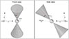 |
Fig. E.1. Schematic representation of the outflow geometry parametrization described in Appendix E.1.3, taken from Pessa et al. (2024). The figure illustrates the front (left) and side (right) view of an outflow characterized by an arbitrary O.A., P.A. = 90° and R.A. = 45°. The opening angle represents the angle between the axis and the surface of each outflow cone, the position angle corresponds to the angle of the outflow with respect to the horizontal axis, in the plane of the sky, and the rotation angle measures the rotation of the outflow in the plane defined by x = 0, with respect to the y-axis. The red line shows the cone axis. The observer is located at a large positive z value. |
E.1.4. PSF and LSF convolution
Accounting for instrumental LSF and PSF is essential for a meaningful comparison between our model and the observed data. The LSF describes the spectral broadening of a given spectral line due to instrumental effects, and the PSF characterizes the spatial broadening of the light distribution of a point-like source in the detector.
The MUSE LSF is modeled as a Gaussian function, whose width was measured by fitting a Gaussian to a set of sky lines in Bacon et al. (2017). The FWHM of the LSF varies smoothly with wavelength, as a second-degree polynomial:
 (E.12)
where λ and FWHM are both in Å.
On the other hand, the MUSE PSF is accurately described by a circular Moffat function with a fixed β and a FWHM that varies linearly with wavelength. For MUSCATEL, the FWHM and β values were determined based on available stars in the field.
The PSF of the MUSCATEL data are well characterized by a Moffat function with β = 2.6 and a FWHM that decreases linearly with wavelength, ranging from a median value of 0.71 ± 0.13 arcseconds on the bluest side of the MUSE wavelength range to 0.50 ± 0.11 arcseconds at the reddest end of the wavelength range. For each galaxy, we adopt the corresponding FWHM based on its MUSCATEL field and the wavelength at which the Mg II transition is observed.
E.2. Fitting method
E.2.1. Modeled signal
We use the model described in the previous section to fit the Mg II emission of our sample galaxies. We consider the wavelength interval around the Mg II transition, approximately the 2790 - 2809 Å range (rest-frame), modeling the two Mg II transitions simultaneously. For some galaxies, the modeled wavelength interval is slightly larger or smaller, if they exhibit, for instance, a broader spectral profile, contamination due to sky emission lines, or a nearby galaxy (in projected distance) that would require truncating the wavelength range. We fit the Mg II emission profile in a circular field of view with a radius of  , which corresponds to 26 − 30 kpc at redshifts 0.7 − 2.2, respectively.
We model the Mg IIλλ2796, 2803 transitions at their corresponding rest-frame velocities, using the same set of parameters to model both transitions, except for τ0. This is because the oscillator strength of Mg IIλ2796 is essentially two times larger than that of Mg IIλ2803 (Kelleher & Podobedova 2008), and thus we used an optical depth of τ = τ0/2 for Mg IIλ2803, as the optical depth depends linearly on the oscillator strength
E.2.2. Description of the fitting
To find the best-fitting parameters for the MUSE data of our sample galaxies, we used a Markov chain Monte Carlo (MCMC) analysis implemented in the EMCEE python package (Foreman-Mackey et al. 2013). For each MCMC step, we compute a model cube and the respective likelihood of the used set of parameters.
We used broad, uninformative priors for most of the outflow parameters described in Appendix E.1:
 (E.13)
 (E.14)
 (E.15)
 (E.16)
 (E.17)
where 𝒩(μ, σ) stands for a Normal distribution with mean μ and standard deviation σ. ℒ𝒰(a, b) and 𝒰(a, b) stand for Log-Uniform and Uniform distributions, within the (a, b) intervals, respectively. This is our standard setup of priors. However, for some galaxies we modified these priors in subsequent runs, for instance, if a posterior distribution converges toward the edge of a prior.
For R0, we chose a prior distribution tailored to each individual galaxy. As described in previous sections, R0 corresponds to the launching radius of the galactic wind and should be on the same order as the size of the stellar component of each galaxy. Thus, we used GALFIT (Peng et al. 2002, 2010) to fit a Sérsic model to the HST F814W image of each galaxy, which should be dominated by stellar continuum emission, to obtain a first estimation of the galaxy size, parametrized by the half-light radius of the Sérsic profile. Then, we chose a normal prior for R0 centered on this half-light radius, with standard deviation of 1 kpc, namely:
 (E.18)
Thus, we exclude scenarios where R0 is much larger or much smaller than the actual size of a given galaxy. For galaxies with more irregular geometries, where the size is less constrained by a simple Sérsic model, we use a broader prior, with a standard deviation of 2 kpc instead. The continuum HLR measured for each galaxy is reported in Table D.1.
An additional parameter Δv accounts for any kinematic offset between the systemic velocity and the P-Cygni emission. Its prior is given by
 (E.19)
and it has units of km s−1. For the geometric parameters, we also use completely agnostic priors, namely,
 (E.20)
 (E.21)
 (E.22)
in units of degrees. Finally, we included an additional term f to account for the existence of additional variance in the data. The extra variance (σ) is proportional to the model such that:
 (E.23)
where M is the value of the model, evaluated in the independent variable, given a set of parameters. The prior on f is given by
 (E.24)
We used 22 MCMC chains to sample the posterior distributions, each with 6000 iterations. We discard 500 burn-in iterations before convergence for each chain. The convergence of the MCMC chains is ensured by using the  criterion (Gelman & Rubin 1992).
Appendix F: Fraction of galaxies in our sample for different exposure times
In Sec. 3.3.2 we show how the presence of a Mg II traced galactic-scale outflow correlated with host-galaxy properties, for our full sample. Here, we investigate the role of the depth of the field in the prevalence of the outflows. Figure F.1 shows the SFR distribution of our parent and final sample of galaxies, and the ratio between the number of galaxies in both samples as a function of the galaxy SFR. Same as the top-right panel of Fig. 6, but now separated by depth of the MUSCATEL fields (e.g., SF, MF, and DF). While the trend with SFR is qualitatively the same for the different depth levels (i.e., higher prevalence of galactic-scale outflows in higher SFR galaxies), the absolute fraction of galaxies that exhibit an outflow is significantly higher for the deeper fields, compared to the shallow field.
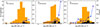 |
Fig. F.1. Comparison of the SFR distributions for our final sample of galaxies (black) and our parent sample (orange), separated by depth of the field (SF, MF, and DF; see MUSCATEL description in Sec. 2.1). The blue line shows the fraction of galaxies from the parent sample in our final sample, in each SFR bin. The right-side y-axis indicates the fraction shown by the blue line. In the top-left corner of each panel is indicated the field depth, and the number of galaxies in the final/parent sample. |
All Tables
Summary of the main properties of the galaxies from our final sample (see Sec. 3 for details on our sample selection).
Summary of the best-fitting model parameters obtained for each one of our sample galaxies.
All Figures
|
Fig. 1. Stellar mass distribution of our preliminary sample of galaxies. The sample consists of 89 galaxies drawn from the MUSCATEL survey that exhibit Mg II in emission or absorption or a P-Cygni profile, determined after a careful inspection of their integrated spectra and their continuum-subtracted Mg II pseudo-narrowband image. A direct S/N threshold has not been applied. Each stacked histogram shows the distribution of the galaxies that belong to each one of the depth levels of the MUSCATEL survey (shallow field, medium field, and deep field; see Sec. 2), indicated in the top-left part of each panel. The black line shows the distribution of the full preliminary sample in all the panels. Stellar masses are calculated via SED fitting, as described in Sec. 2.2. The stacked histograms are color coded by the different spectral profiles shown in Mg II, as indicated in the legend. |
| In the text | |
|
Fig. 2. Significance of the extended Mg II emission, stellar mass, and redshift distribution for the galaxies in our preliminary sample that exhibit a P-Cygni profile in Mg II. Left: significance of the extended Mg II emission in terms of its spatially integrated S/N for the 50 galaxies in our preliminary sample that exhibit a P-Cygni profile in Mg II. We further removed from our preliminary sample those galaxies where the integrated S/N of the modeled emission is lower than 3σ (indicated with a vertical dashed red line). Middle: stacked histogram that shows the stellar mass distribution of galaxies in the preliminary sample with a P-Cygni profile in Mg II. The gray histogram shows the stellar mass distribution of those galaxies where the significance of the Mg II emission is above the 3σ threshold. The black histogram shows the stellar mass distribution of galaxies below this significance threshold. Right: same as middle panel, but for the redshift distribution of the sample galaxies. |
| In the text | |
|
Fig. 3. Star formation rate as a function of stellar mass for our sample galaxies. Both quantities were obtained via SED fitting (see Sec. 2.2). Our final sample of 47 galaxies that exhibit a P-Cygni profile and a significant detection of modeled extended emission is shown with squares, color coded by redshift. The preliminary sample is shown as dark gray circles, and the original parent sample is shown as smaller light gray dots. For reference, we show the SFMS as measured by Popesso et al. (2023) for z = 1 (solid) and z = 2 (dashed) by collecting different measurements of the SFMS for a wide range of redshifts. |
| In the text | |
|
Fig. 4. Compilation of continuum-subtracted Mg II pseudo-narrowband images (gray color scale) and HST F814W images (blue color scale, probing the stellar light) for our final sample of galaxies that exhibit a P-Cygni profile in Mg II as well as a significant detection of extended Mg II emission. Galaxies are sorted by stellar mass in descending order. The continuum-subtracted Mg II pseudo-narrowband images were computed by collapsing the MUSE data across the wavelength axis for wavelengths that enclose the full P-Cygni profile of the Mg II doublet for a field of view of 80 × 80 kpc2. The brown circle in the bottom-left part of the panel shows the size of the MUSE PSF. The black contours show the 1-σ and 2-σ detection levels of Mg II net emission in the pseudo-narrowband images. The red contours show the 2-σ and 4-σ levels of Mg II net absorption in the pseudo-narrowband images. For visualization purposes, the continuum-subtracted Mg II pseudo-narrowband images have been smoothed using a Gaussian kernel with a FWHM of 1 arcsec. For each galaxy, we also show the radial profile of the Mg II emission as observed in the data (solid) and after correcting by self-absorption using our best-fitting model (dashed; see Sec. 4). The vertical dotted brown line shows the half-light radius measured for the self-absorption corrected radial profiles. The inset shows the Mg II spectrum extracted from the MUSE data cube for each galaxy, across the full modeled region (black) and a small central aperture of radius |
| In the text | |
|
Fig. 5. Comparison of the SFR values derived for our sample galaxies obtained via SED fitting (see Sec. 2.2 for details) and from the [O II] luminosity of each galaxy (see Sec. 3.3.1). The black squares show the SFR values for galaxies in our final sample, and the gray dots show the SFR values for galaxies in the preliminary sample, for the subset of galaxies at z ≲ 1.48, where the [O II] doublet falls well within the MUSE wavelength range. The red line shows the identity for reference. Table D.1 provides these measurements for each galaxy in our final sample. |
| In the text | |
|
Fig. 6. Comparison of the stellar mass, SFR, sSFR, and age distributions for our final sample of galaxies (black) and our parent sample (orange). The blue line shows the fraction of galaxies from the parent sample in our final sample in each bin of the relevant quantity for each panel. The right side y-axis indicates the fraction shown by the blue line. |
| In the text | |
|
Fig. 7. Distribution of the sizes (in terms of HLR) of the Mg II halos. The halos were corrected by self-absorption before measuring their HLR using the absorption component of the best-fitting model. The radial profiles of the absorption-corrected Mg II emission halos are shown with a dashed line in Fig. 4. The HLR of each galaxy is provided in Table D.1. |
| In the text | |
|
Fig. 8. Summary of the comparison of the observed and best-fitting model Mg II spectral profile and continuum-subtracted pseudo-narrowband images for an example galaxy in our final sample (M0416-SF7-012). The top-left panel shows the cutout of the HST F814W image around the galaxy, of 7 arcsec2 size. The top-middle panels show the observed (middle-left) and best-fitting model (middle-right) continuum-subtracted Mg II pseudo-narrowband images. The pseudo-narrowband images were created by collapsing the cubes across the wavelength axis, for wavelengths that enclose the full P-Cygni profile of the Mg II doublet. The size of the pseudo-narrowband images is the same as that of the HST F814W cutout. The two panels show net Mg II emission in black and net Mg II absorption in red. The residuals between both images are shown in the top-right panel. The rest of the panels show the integrated Mg II spectra on different annular (and circular) apertures for the data (solid) and best-fitting model (dashed) cubes. The residuals are shown in the small panels below, in units of standard deviations. The vertical dotted brown lines indicate the rest-frame wavelength of the Mg II doublet. The blue circle in the top-left panel shows the size of the full modeled region, and the black spectrum corresponds to the spectrum integrated over it. The rest of the panels that show colored spectra (and residuals) correspond to the comparison of the spectra extracted from the data and model cubes, in different annular and circular (in the case of the magenta spectra) apertures. In the legend of each panel, the inner and outer radii of the annular apertures are indicated. The color of the spectra in each panel matches the color of the circle in the top-left panel, which corresponds to the outer radii of its annular (or circular) aperture. The nearly horizontal dotted lines in each panel indicate the approximate continuum level. |
| In the text | |
|
Fig. 9. Distribution of the best-fitting model parameters for our sample galaxies. The parameters of the model are described in detail in Appendix E.1. For R.A., we only included galaxies with non-isotropic outflows (O.A. < 75°), and for P.A., we considered only galaxies with non-isotropic outflows (O.A. < 75°) that are also not seen nearly face on (R.A. < 75°). The median and standard deviation of each distribution are indicated in each corresponding panel. The best-fitting parameters and their uncertainties obtained for each galaxy are provided in Table D.2. |
| In the text | |
|
Fig. 10. Correlation of the best-fitting model parameters obtained with our outflow modeling scheme (see Appendix E.1) with the stellar mass of each galaxy, derived via SED fitting (see Sec. 2.2). The plots are color coded by the size of the Mg II halo of each galaxy, reported in Sec. 4, with green colors indicating halos in the extended regime of the distribution, and pink colors indicating more compact halos. The blue squares in the top-left panel indicate galaxies with a more robustly constrained τ0. For R.A., we only included galaxies with non-isotropic outflows (O.A. < 75°), and for P.A., we only considered galaxies with non-isotropic outflows (O.A. < 75°) that are also not seen nearly face on (R.A. < 75°). |
| In the text | |
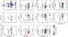 |
Fig. 11. Same as Fig. 10, but for the sSFR derived via SED fitting for our sample galaxies. |
| In the text | |
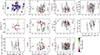 |
Fig. 12. Same as Fig. 10, but for the ΣSFR estimated for our sample galaxies. |
| In the text | |
|
Fig. 13. Size of the Mg II emission halos after correcting by self-absorption as described in Sec. 4. The left panel shows the sizes of the Mg II emission halos as a function of the stellar mass of each galaxy, derived via SED fitting. The inset in the left panel shows a zoom-in to the HLR versus stellar mass relation for only those galaxies with HLR < 8 kpc. The right panel shows the ratio between the size of the Mg II emission halos and the size of the stellar component, as a function of the stellar mass of our sample galaxies. The horizontal dashed gray line shows the ratio of one for reference. |
| In the text | |
|
Fig. 14. Comparison of the orientation derived for the outflow (R.A.) with that inferred for the stellar disk of each galaxy from the HST F814W image using GALFIT. The dashed red line shows the identity, that is, when the inclination of the galaxy and the inclination of the outflow are the same. For a face-on polar outflow, both inclinations would be ∼90°, and for an edge-on polar outflow, both would be ∼0°. We have excluded from the figure galaxies that exhibit a nearly isotropic outflow (O.A. > 75°), as well as galaxies for which the inclination measured with GALFIT was too uncertain due to their complex surface brightness profile. The orange squares indicate galaxies with a measured continuum HLRs > 2 kpc. The formal uncertainties of the inclination provided by GALFIT are < 1°. |
| In the text | |
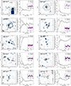 |
Fig. A.1. Continuation of Fig. 4. |
| In the text | |
|
Fig. A.1. (Continued.) |
| In the text | |
|
Fig. A.1. (Continued.) |
| In the text | |
|
Fig. A.1. (Continued.) |
| In the text | |
|
Fig. B.1. Comparison between the observed and best-fitting model cubes, in terms of the continuum-subtracted pseudo-narrowband images and spectra extracted from annular apertures for four sample galaxies. Each set of panels corresponds to one galaxy, following the same layout as in Fig. 8 (see caption of Fig. 8 for a full description of each panel). |
| In the text | |
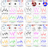 |
Fig. B.2. Same as Fig. B.1, but for four other galaxies in our sample. |
| In the text | |
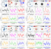 |
Fig. B.3. Same as Fig. B.1, but for four other galaxies in our sample. |
| In the text | |
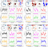 |
Fig. B.4. Same as Fig. B.1, but for four other galaxies in our sample. |
| In the text | |
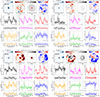 |
Fig. B.5. Same as Fig. B.1, but for four other galaxies in our sample. |
| In the text | |
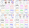 |
Fig. B.6. Same as Fig. B.1, but for four other galaxies in our sample. |
| In the text | |
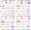 |
Fig. B.7. Same as Fig. B.1, but for four other galaxies in our sample. |
| In the text | |
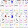 |
Fig. B.8. Same as Fig. B.1, but for four other galaxies in our sample. |
| In the text | |
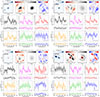 |
Fig. B.9. Same as Fig. B.1, but for four other galaxies in our sample. |
| In the text | |
|
Fig. B.10. Same as Fig. B.1, but for four other galaxies in our sample. |
| In the text | |
|
Fig. B.11. Same as Fig. B.1, but for four other galaxies in our sample. |
| In the text | |
|
Fig. B.12. Same as Fig. B.1, but for three other galaxies in our sample. |
| In the text | |
|
Fig. C.1. Comparison between data and model cube for two galaxies in our sample (AS1063-MF3-004 and AS1063-MF3-091) that are physical neighbors, with a projected separation of ∼18 kpc, and a velocity difference of ∼160 km s−1, whose Mg II halo could potentially be interacting and thus deviating from a simple outflow model. The set of panels on the left side of the figure shows the data and best-fitting model comparison for AS1063-MF3-004, and the right set of panels shows the same for AS1063-MF3-091. The layout of each set of panels is the same as in Fig. C.3, comparing the continuum-subtracted Mg II pseudo-narrowband images and the spectra extracted from annular apertures from the data and best-fitting model cube. The nearby galaxies have been masked during the fitting of each individual galaxy. |
| In the text | |
|
Fig. C.2. Comparison between data and model cube for one of our sample galaxies (A2744-DF-013) whose Mg II emission halo exhibits characteristics that are inconsistent with our purely outflow emission model. By including an additional inflow-absorbing contribution to the model, we are able to reproduce the data more closely. The parameterization of the inflow component is detailed in the main text (see Sec C.2). The set of panels on the left side of the figure shows the data and best-fitting model comparison for A2744-DF-013, using our fiducial outflow-only model described in Appendix E.1. The right set of panels shows the same for our outflow+inflow model. The layout of each set of panels is the same as in Fig. C.3, comparing the continuum-subtracted Mg II pseudo-narrowband images and the spectra extracted from annular apertures from the data and best-fitting model cube. |
| In the text | |
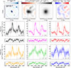 |
Fig. C.3. Same as Fig. 8, but for another galaxy in our sample (AS1063-MF2-011). |
| In the text | |
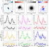 |
Fig. C.4. Same as Fig. 8, but for another galaxy in our sample (AS1063-DF-109). |
| In the text | |
|
Fig. E.1. Schematic representation of the outflow geometry parametrization described in Appendix E.1.3, taken from Pessa et al. (2024). The figure illustrates the front (left) and side (right) view of an outflow characterized by an arbitrary O.A., P.A. = 90° and R.A. = 45°. The opening angle represents the angle between the axis and the surface of each outflow cone, the position angle corresponds to the angle of the outflow with respect to the horizontal axis, in the plane of the sky, and the rotation angle measures the rotation of the outflow in the plane defined by x = 0, with respect to the y-axis. The red line shows the cone axis. The observer is located at a large positive z value. |
| In the text | |
|
Fig. F.1. Comparison of the SFR distributions for our final sample of galaxies (black) and our parent sample (orange), separated by depth of the field (SF, MF, and DF; see MUSCATEL description in Sec. 2.1). The blue line shows the fraction of galaxies from the parent sample in our final sample, in each SFR bin. The right-side y-axis indicates the fraction shown by the blue line. In the top-left corner of each panel is indicated the field depth, and the number of galaxies in the final/parent sample. |
| In the text | |
Current usage metrics show cumulative count of Article Views (full-text article views including HTML views, PDF and ePub downloads, according to the available data) and Abstracts Views on Vision4Press platform.
Data correspond to usage on the plateform after 2015. The current usage metrics is available 48-96 hours after online publication and is updated daily on week days.
Initial download of the metrics may take a while.