| Issue |
A&A
Volume 701, September 2025
|
|
|---|---|---|
| Article Number | A128 | |
| Number of page(s) | 33 | |
| Section | Stellar structure and evolution | |
| DOI | https://doi.org/10.1051/0004-6361/202554370 | |
| Published online | 09 September 2025 | |
Early light curve excess in Type IIb supernovae observed with ATLAS
Qualitative constraints on progenitor systems
1
Instituto de Astrofísica, Departamento de Física, Facultad de Ciencias Exactas, Universidad Andrés Bello, Fernández Concha 700, Las Condes, Santiago RM, Chile
2
Millennium Institute of Astrophysics, Nuncio Monseñor Sotero Sanz 100, Of. 104, Providencia, Santiago, Chile
3
European Southern Observatory, Alonso de Córdova 3107, Vitacura, Santiago, Chile
4
Instituto de Alta Investigación, Universidad de Tarapacá, Casilla 7D, Arica, Chile
5
Data and Artificial Intelligence Initiative (IDIA), Faculty of Physical and Mathematical Sciences, Universidad de Chile, Santiago, Chile
6
Center for Mathematical Modeling, Universidad de Chile, Beauchef 851, Santiago 8370456, Chile
7
Department of Physics, University of Oxford, Keble Road, Oxford OX1 3RH, UK
8
Astrophysics Research Centre, School of Mathematics and Physics, Queen’s University Belfast, N. Ireland BT7 1NN, United Kingdom
9
Space Telescope Science Institute, 3700 San Martin Drive, Baltimore MD 21218, USA
10
Physics and Astronomy Department, Johns Hopkins University Baltimore MD 21218, USA
11
Astronomical Observatory Institute, Faculty of Physics and Astronomy, Adam Mickiewicz University, ul. Słoneczna 36, 60-286 Poznań, Poland
12
South African Astronomical Observatory, Cape Town 7925, South Africa
13
Department of Physics, Stellenbosch University, Stellenbosch 7602, South Africa
⋆ Corresponding author: This email address is being protected from spambots. You need JavaScript enabled to view it.
Received:
4
March
2025
Accepted:
11
June
2025
Abstract
Context. Type IIb supernovae (SNe IIb) often exhibit an early light curve excess (EE) preceding the main peak powered by 56Ni decay. The physical origin of this early emission remains an open question. Among the proposed scenarios, shock cooling (SC) emission, resulting from the interaction of the shock wave with extended envelopes, is considered the most plausible mechanism. However, the occurrence rate of such events has yet to be reliably constrained.
Aims. This study aims to quantify the frequency of EE in SNe IIb and investigate its physical origin by analysing optical light curves from the Asteroid Terrestrial-impact Last Alert System (ATLAS) survey, ultimately providing qualitative constraints on their progenitor systems.
Methods. We identified 74 potential SNe IIb from 153 spectroscopically classified events reported in the Transient Name Server (TNS), observed by ATLAS with peak fluxes exceeding 150 μJy (18.46 mag) and explosion epoch uncertainties below six days. Using a spectral reclassification method, we selected a sample of 66 SNe IIb and a cleaned sample of 59 SNe IIb for analysis. We then applied light curve model fitting and outlier analysis to identify objects exhibiting EE emission and studied their photometric properties.
Results. We identify 20 SNe IIb with EE, corresponding to a frequency of approximately 30.5% to 50%, the higher value being obtained under the most stringent observational data-quality cuts. The duration and colour evolution of the early excess support its interpretation as shock cooling in extended envelopes. We also find that EE SNe IIb exhibit faster post-peak declines than non-EE events, while both groups show similar peak absolute magnitudes and rise-time distributions.
Conclusions. Our findings suggest that EE and non-EE SNe IIb likely share similar initial progenitor masses but differ in their ejecta properties, potentially due to varying degrees of binary interaction. This study constrains EE SNe frequency and photometric properties, paving the way for future theoretical work, such as hydrodynamical modelling of EE SNe light curves, which could corroborate these results and contribute to constraining the evolutionary pathways of SNe IIb progenitor systems.
Key words: supernovae: general
© The Authors 2025
 Open Access article, published by EDP Sciences, under the terms of the Creative Commons Attribution License (https://creativecommons.org/licenses/by/4.0), which permits unrestricted use, distribution, and reproduction in any medium, provided the original work is properly cited.
This article is published in open access under the Subscribe to Open model. This email address is being protected from spambots. You need JavaScript enabled to view it. to support open access publication.
1. Introduction
Core-collapse supernovae (CCSNe) are the explosions of stars in their final evolutionary stages, with zero-age main sequence (ZAMS) masses, MZAMS ≳ 8 − 10 M⊙ (e.g. Heger et al. 2003; Smartt 2009), leaving a neutron star or a black hole as a remnant. Among CCSNe, stripped-envelope supernovae (SESNe – Types Ic, Ib, and IIb) form a subcategory, where the progenitor loses part of its envelope prior to the explosion (Clocchiatti et al. 1996). Within the SESNe class, SNe IIb exhibit hydrogen features at early times that disappear a few weeks after the explosion, as helium lines begin to emerge in the spectrum (e.g. Filippenko et al. 1993; Filippenko 1997). SN IIb progenitors are thought to retain part of their hydrogen envelope, with estimated masses ranging between a few hundredths up to to one solar mass (e.g. Smith et al. 2011; Sravan et al. 2019; Gilkis & Arcavi 2022). The dominant mechanism responsible for stripping the progenitor’s envelope prior to explosion remains uncertain. However, the likely mechanisms include stellar winds in more massive (MZAMS ≳ 20 M⊙) isolated stars (e.g. Smith & Owocki 2006; Puls et al. 2008) and mass transfer in close binary systems involving a less massive (MZAMS ≲ 17 M⊙) progenitor star (e.g. Claeys et al. 2011; Benvenuto et al. 2013).
Type IIb supernovae typically display single-peaked, bell-shaped light curves and reach this peak approximately 20 days after the explosion (e.g. Lyman et al. 2016; Drout et al. 2011; Rodríguez et al. 2023), with the luminosity mainly powered by the radioactive decay of 56Ni → 56Co → 56Fe (Woosley et al. 1994). However, Rodríguez et al. (2024) have recently argued that the luminosity of most SESNe (including SNe IIb) cannot be explained solely by 56Ni decay. Regardless of the primary power source (e.g. 56Ni, central engine, or circumstellar material interactions), statistical studies have show that SNe IIb generally exhibits single-peaked light curves (e.g. Taddia et al. 2018; Rodríguez et al. 2024). Nevertheless, some SNe IIb display an additional early excess (EE) preceding the 56Ni peak. This feature has been observed in several SNe IIb, including SN 1993J (Woosley et al. 1994), SN 2011fu (Kumar et al. 2013), SN 2011dh (Arcavi et al. 2011), SN 2011hs (Bufano et al. 2014), SN 2013df (Van Dyk et al. 2014; Morales-Garoffolo et al. 2014), SN 2016gkg (Bersten et al. 2018; Arcavi et al. 2017), SN 2017jgh (Armstrong et al. 2021), ZTF18aalrxas (Fremling et al. 2019), SN 2020bio (Pellegrino et al. 2023), SN 2021zby (Wang et al. 2023), and SN 2024uwq (Subrayan et al. 2025).
Several works propose that the early flux excess observed in some Type IIb SNe (hereafter EE SNe), which precedes the 56Ni peak and produces double-peaked light curves, arises from different physical mechanisms. For instance, double 56Ni distributions could produce an early luminosity peak through jet-like outflows that eject nickel-rich material into low-opacity regions (Orellana & Bersten 2022). Alternatively, the strength and shape of the first peak could be affected by Thomson scattering and chemical mixing in double-peaked SNe IIb light curves (Park et al. 2024). However, for the 11 EE SNe listed above, the most widely accepted explanation involves the interaction of the shock wave generated during core collapse with an extended envelope. This interaction results in a shock-heated envelope that radiates as it cools (e.g. Soderberg et al. 2012; Nakar & Piro 2014; Van Dyk et al. 2014; Piro 2015; Sapir & Waxman 2017; Piro et al. 2021).
Several studies have investigated the physical conditions required to produce double-peaked light curves, assuming their origin in shock cooling (SC) emission, and they have shown that extended envelopes are essential. Using analytical approximations, Nakar & Piro (2014) demonstrated that hydrogen-rich low-mass (∼0.06 M⊙) extended envelopes can produce double-peaked light curves. Piro (2015) refined this model, showing that a more massive and extended envelope prolongs the shock propagation and results in a brighter, more pronounced early peak. Similarly, Sapir & Waxman (2017) showed that hydrogen-dominated envelopes with masses below 1 M⊙, modelled using polytropic density profiles, can also reproduce early light curve peaks. Piro et al. (2021) developed an updated analytic model for SC emission that incorporates a more realistic two-component density structure. They showed that low-mass (∼0.01 − 0.1 M⊙), extended envelopes (∼100 − 300 R⊙) naturally produce double-peaked light curves. Supporting these insights, hydrodynamic simulations of SN 2011dh by Bersten et al. (2012) suggest that the double-peaked light curve of SN 2011dh resulted from a low-mass extended envelope (Menv ≈ 0.1 M⊙). Dessart et al. (2018) further proposed that progenitors with a core-halo structure, where 95% of the mass is confined within 10% of the stellar radius, can produce double-peaked light curves due to their tenuous and extended envelopes.
Most recently, Dessart et al. (2024) simulated CCSNe light curves originating from progenitors in binary systems. Their model used fixed values for the explosion energy and 56Ni mass. The primary star had a ZAMS mass of 12 M⊙ and a mass ratio of 0.9 relative to the companion, while the initial binary period was varied. These variations led to progenitors with different hydrogen masses and envelope properties, producing a diversity of light curve morphologies, including double-peaked light curves consistent with SNe IIb.
The binary progenitor scenario is currently considered the most plausible origin for SNe IIb. Direct and indirect evidence support this hypothesis. Post-explosion images have revealed companion stars for SN 2011dh (Folatelli et al. 2014), SN 2001ig (Ryder et al. 2018), and SN 1993J (Maund et al. 2004). In addition, pseudo-spectral energy distributions from pre-explosion images of SN 2008ax indicate either a single B-type star or a binary system with a lower-mass progenitor and a main-sequence O9-B0 companion (Folatelli et al. 2015).
Theoretical studies suggest that SNe IIb may originate from either single or binary progenitor systems. Single-star models require high ZAMS masses (20 − 26 M⊙) to strip the hydrogen envelope through strong stellar winds (Georgy 2012; Sravan et al. 2019). However, only mass transfer from lower-mass primaries in close binaries can reproduce the observed properties of SNe IIb, including their helium-core masses, under specific parameter configurations, thus highlighting binary interactions as a plausible evolutionary pathway for SNe IIb (Claeys et al. 2011; Yoon et al. 2017; Sravan et al. 2019, 2020).
Additional evidence from X-ray and radio observations has reveals circumstellar densities higher than those expected from single-star mass loss, suggesting that binary interactions could play an important role in shaping the environments of SNe IIb (e.g. Sravan et al. 2020). Furthermore, the observed correlation between progenitor radius and mass-loss rate is naturally explained by binary interaction via mass transfer (Ouchi & Maeda 2017), further supporting the binary progenitor scenario. Moreover, more than 70% of massive stars are estimated to interact in binaries during their evolution (e.g. Sana et al. 2012). This fraction suggests that binary star systems could be the progenitors of SNe IIb and that binary interactions could produce the properties of SNe IIb progenitors (for further details, see Sravan et al. 2019, 2020, and references therein).
In this paper, we aim to quantify the fraction of SNe IIb that exhibit an EE preceding the main peak using data from the ATLAS survey (Tonry et al. 2018), which provides one of the highest cadences currently available among all-sky surveys. In addition to quantifying the EE frequency, we characterise the light curves of EE SNe and SNe IIb without the EE (hereafter non-EE SNe) using parameters such as post-peak decline (ΔM15, the difference in magnitude between the peak and 15 days after the peak), peak absolute magnitude (Mpeak), and rise time (trise, time between the explosion and the 56Ni light curve peak). We interpret these light curve parameters in terms of explosion and progenitor properties, including 56Ni mass and ejecta mass (Mej), based on correlations reported in the literature (Drout et al. 2011; Wheeler et al. 2015; Lyman et al. 2016; Prentice et al. 2016, 2019; Dessart et al. 2016; Rodríguez et al. 2023). Finally, we attempt to understand and constrain the different progenitor scenarios that can explain the observed light curve properties of EE and non-EE SNe IIb.
This paper is structured as follows. In Sect. 2 we describe the data selection, photometric cleaning process, spectroscopic reclassification, and identification of peculiar or misclassified SNe IIb. Sect. 3 introduces the methodology for detecting the EE, including the estimation of explosion epochs and the process of fitting light curves and identifying the EE. Sect. 4 presents the results, including model performance, EE frequency, light curve characterisation, and a comparison between EE and non-EE SNe IIb. It also analyses EE duration and colour, and assesses the robustness of the findings. Sect. 5 presents a correlation analysis of the light curve parameters. In addition, it provides a qualitative physical interpretation of the light curve parameter distributions, discusses implications for progenitor systems based on the conditions required to produce double-peaked light curves, and outlines scenarios that could lead to extended envelopes. Finally, Sect. 6 summarises the main conclusions of this study.
2. Data sample, cleaning, and reclassification
As of 3 October 2024, the Transient Name Server1 (TNS) had reported a total of 233 spectroscopically classified SNe IIb, 154 of which had been observed by ATLAS (Smith et al. 2020).
ATLAS is a sky survey funded by the National Aeronautics and Space Administration (NASA) and operated by the University of Hawaii. It consists of four telescopes: two in Hawaii, one in Chile, and another in South Africa. Although ATLAS was designed primarily to detect near-Earth asteroids, its high-cadence and deep imaging strategy makes it an excellent facility to discover and photometrically follow transient events. With its large field of view (55 deg2), ATLAS can scan the entire observable sky every one or two days, depending on the weather conditions, with four exposures obtained on individual fields on each night (Tonry et al. 2018). The survey operates in two bands: cyan (c) and orange (o), corresponding approximately to the g+r and r+i filters from Pan-STARRS (Tonry et al. 2018), covering wavelength ranges of 420–650 nm and 560–820 nm, respectively. During dark time2, the ATLAS-o band reaches a limiting flux of ∼43.65 μJy (corresponding to a magnitude of 19.8).
We downloaded forced photometry of all SNe IIb from the ATLAS Forced Photometry server (Shingles et al. 2021) and applied the ATClean tool (Rest et al. 2023, 2025) to perform photometric data cleaning. ATClean employs a data-cleaning methodology that includes several steps. First, it analyses control light curves (CLCs) defined as forced photometry in a 17″ circular aperture around the SN to measure the sky flux (see Figure 1 in Rest et al. 2025) and estimates additional noise. Next, chi-square PSF fitting ( ) and flux uncertainty cuts are applied. Then, SN photometry is averaged over the four measurements obtained each night. A detailed description of the methodology and parameters used in ATClean is summarised in Appendix A.
Panels (a) and (b) in Figure 1 show the result of applying ATClean to the SN 2021zby light curve. In this work, we used only the o-band since the c-band is significantly less sampled than the o-band, as can be seen in Figure 1.
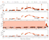 |
Fig. 1. Data cleaning and explosion epoch estimation example for SN 2021zby. The panels, labelled as a, b, c, and d from top to bottom, present different stages of the analysis (we detail a and b in Section 2 and c and d in Section 3). Red and grey dots represent photometry in the o and c bands, respectively. Panel (a) shows the raw ATLAS forced photometry. Panel (b) presents the photometry after applying the ATClean methodology detailed in Section 2. Panel (c) shows the pre-SN photometry, where the red region highlights the relevant data, and the sky blue and brown dashed lines represent the 3 and 1.5 σpre − SN values, respectively. In Panel (d), green and black star symbols represent the last non-detection and discovery, which we use to estimate the explosion time. |
From the 154 SNe IIb observed by ATLAS and reported in the TNS, we selected 74 with peak fluxes fpeak > 150 μJy (18.46 mag) to measure key light curve parameters such as ΔM15. SNe IIb exhibit a mean post-peak decline of ΔM15 = 0.72 ± 0.2 mag (Rodríguez et al. 2023), which corresponds to a flux of approximately 78 μJy. Thus, selecting objects with fpeak > 150 μJy ensures that the flux remains above the ATLAS detection limit of 43.65 μJy (19.8 mag) at 15 days after peak, allowing accurate measurement of the post-peak decline.
The sample of 74 SNe represents our potential sample of SNe IIb as classifications reported in the TNS are not always reliable, depending on the individual reporters and the available data quality. Therefore, we reclassified the 74 SNe using spectral-matching classification tools. From our methodology described in Appendix B.1, we identified six objects potentially misclassified as SNe IIb: 2018jee (II-P), 2019rn (Ic), 2020tjd (II-P), 2021rjj (Ib), 2022ngb (Ib), and 2023mti (II-P). In addition, SN 2019lgc lacks publicly available spectra for reclassification. Consequently, we excluded this object from our analysis sample.
Our reclassification does not guarantee that all reclassified objects are indeed SNe IIb, as most have only a single available spectrum, preventing a robust spectroscopic time-series classification analysis. Consequently, for the 67 SNe reclassified as SNe IIb, we identify objects that do not follow the typical photometric behaviour of SNe IIb. Based on the defined method described in Appendix B.2, we identify SN 2022ytx, which, despite having a good spectroscopic match to a SN IIb, exhibits photometric properties inconsistent with normal SNe IIb (see Appendix B.2.1). Furthermore, we identify four objects (SN 2019hte, SN 2021iiu, SN 2022fzf, SN 2022W) that display a transitional photometric behaviour between SNe II and IIb.
For this study, we have defined a sample of 66 objects, from which we excluded six misclassified events based on our spectral reclassification and removed SN 2022ytx. This sample retains the four objects with transitional light curves between SNe II and IIb. However, we exclude them from a cleaned subsample of 59 SNe IIb, which we define to test the robustness of our results in Section 4.5.
It is important to note that the sample used in this work may represent a lower limit to the number of SNe IIb, biasing the derived results, such as EE-SNe frequency. This underestimation may result because some SNe IIb could be misclassified as SNe II (see example in Appendix B.2.2). Additionally, some SNe IIb may be misclassified as SNe Ib if their spectra were obtained at phases when hydrogen features have already disappeared.
Addressing this issue will require first expanding the number of spectra and improving the template libraries of SNe IIb and SNe Ib used in spectral classification tools. It would also involve collecting spectra and light curves to reclassify and analyse the full sample of ∼700 SNe II and ∼130 SNe Ib reported in the TNS and observed by ATLAS. That is beyond the scope of this paper. However, we plan to develop this study in a future work by compiling and analysing all CCSNe reported in the TNS and observed by ATLAS.
3. Shock cooling detection: Methodology
Figure 1 shows an example SN IIb light curve of SN 2021zby, which displays the standard broad peak that is understood to be produced by the decay of 56Ni (Woosley et al. 1994) and an EE preceding the 56Ni peak. In this section, we introduce our statistical methodology for detecting or ruling out the presence of EE in the light curves. We define EE detection by identifying positive photometric outliers (i.e. residuals where the flux exceeds the model prediction) before the light curve maximum, compared to a model that does not reproduce double-peaked light curves.
3.1. Light curve properties: Explosion epoch and point density
Accurate estimation of the explosion epoch and its uncertainty is essential for properly detecting and characterizing early flux excess, given that previously reported cases in the literature have durations ranging from approximately four days (e.g. SN 2011dh; Arcavi et al. 2011) to 12 days (e.g. SN 2021zby; Wang et al. 2023). We estimate the explosion epoch texp and its uncertainty δtexp using pre-explosion SN photometry from ATLAS. Specifically, we determine texp as the midpoint between the last non-detection and the discovery epoch, following standard procedures (e.g. Taddia et al. 2015). A detailed description of the discovery time and last non-detection determination is provided in Appendix C. Figure 1(d) illustrates an example of the estimation of the last non-detection and discovery epochs, while panel (c) shows the pre-SN flux.
Using our selected sample of 66 SNe with peak flux greater than fpeak > 150 μJy (18.46 mag), we analysed the distributions of fpeak, δtexp, ρpeak, and redshift (z), as shown in Figure 2. Here, ρpeak represents the numerical density of points during the rise time, defined as the number of photometric data points between the explosion and the peak divided by the time to peak3. The sample exhibits a mean and median redshift of 0.024, with a mean and median peak brightness of 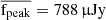 (16.65 mag) and
  (17.85 mag), respectively. The explosion epoch uncertainty has mean and median values of
  days and
  days, respectively. These small uncertainties demonstrate ATLAS’s capability of estimating accurate explosion epochs, which is crucial for studying EE flux in SNe IIb.
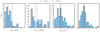 |
Fig. 2. Distributions of fpeak, δtexp, ρpeak, and z for the SNe sample. Red and grey vertical dashed lines indicate the median and mean, respectively. |
3.2. Light curve fitting and EE identification
We detect early flux excess by fitting an analytic function representative of standard SN light curves, where we do not expect additional peaks before the maximum. Consequently, any early-time flux excess will result in positive residuals where the observed flux exceeds the model. We define an EE point as a positive outlier that deviates from the model by more than three times the residual standard deviation (3σr) between texp − δtexp and tpeak, where texp is the explosion time and δtexp is the uncertainty in the explosion time, and tpeak is the time to the light curve peak. Specifically, a data point at time ti is considered a 3σr outlier if its residual, defined as 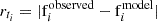 , satisfies rti > 3σr. We adopt a 3σr threshold, corresponding to a deviation with a probability of 0.13% under a normal distribution, thus ensuring a statistically significant departure from the model expectations.
We fit the Supernova Parametric Model (SPM) introduced by Villar et al. (2019), which is a six-parameter analytic model that describes SN light curves that considers factors such as explosion times, initial rise timescales, and post-peak decline rates. It is important to mention that the SPM model is not a physical model based on radiative processes, but an analytical model. We employ the modified version of the SPM as described by Sánchez-Sáez et al. (2021), defined by the following equation
![Mathematical equation: $$ \begin{aligned} F&= \frac{A \left(1 - \beta {\prime } \frac{t - t_{0}}{t_{1} - t_{0}}\right)}{1 + \exp \left(- \frac{t - t_{0}}{\tau _{\mathrm{rise}}}\right)} \left[1 - \sigma \left(\frac{t - t_{1}}{3}\right)\right] \nonumber \\&\quad + \frac{A(1 - \beta {\prime }) \exp \left(- \frac{t - t_{1}}{\tau _{\mathrm{fall}}}\right)}{1 + \exp \left(- \frac{t - t_{0}}{\tau _{\mathrm{rise}}}\right)} \left[\sigma \left(\frac{t - t_{1}}{3}\right)\right], \nonumber \\ \sigma (t)&= \frac{1}{1 + \exp (-t)}\cdot \end{aligned} $$](/articles/aa/full_html/2025/09/aa54370-25/aa54370-25-eq7.gif) (1)
(1)
This modified version includes two key improvements: first, the reparametrisation ensures the function remains positive within a valid range; second, incorporating a sigmoid function alloisationws for a smooth transition between the two components of the model, enabling more effective optimisation and improving parameter estimation. Even though each parameter in the analytical model has a unique effect, degeneracies prevent distinct interpretations of the physical basis of each parameter (Villar et al. 2019). For example, A affects the amplitude; τrise, γ (γ ≡ t1 − t0), and τfall influence the rise, plateau onset, and fall of the light curve, respectively; t0 shifts the light curve in phase; and β′ affects the slope of the plateau.
We estimate the best fit using the Markov Chain Monte Carlo (MCMC) method, which maximises the posterior probability 𝒫(θ|D)∝ℒ(D|θ)π(θ), where ℒ(D|θ) is the likelihood function and π(θ) represents the prior probability of the parameters θ. We employed the Python package emcee (Foreman-Mackey et al. 2013) for this analysis. We defined the input parameter distributions using Gaussian priors 𝒩(μ, σ), where μ is the mean, σ the standard deviation, and boundary conditions (B) restrict the priors to zero probability outside the defined range (see Table 1). The SPM was fitted to the o-band light curves at phases between (texp − δtexp) and 60 days post-explosion, provided the flux exceeded 60 μJy (19.45 mag) to avoid biases near the ATLAS survey’s limiting flux of ∼43.65 μJy (19.8). Best-fit parameter values were derived from the posterior distributions using the median of the samples, with uncertainties estimated as the 16th and 84th percentiles. Figure D.1 in the appendix illustrates an example of the posterior distributions for SN 2022jpx.
Markov Chain Monte Carlo input parameters for the SPM.
Given that the early flux excess could affect our light curve fitting (as the SPM does not account for this feature), we mitigate its influence by iteratively refitting the models after removing all positive 3σr outliers between texp and tpeak, as described in Section 3.2. The refitting process stops at the iteration at which no outliers remain, thus ensuring that our light curve represents the early evolution of normal SNe IIb (without flux excess), which is fundamental to our methodology for detecting flux excess. Figure 3 illustrates an example of the SPM iterative fitting after removing outliers for SN 2022jpx.
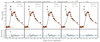 |
Fig. 3. Example of the SPM fit and refitting process for SN 2022jpx. The left panel shows the initial SPM fit, with outliers identified and enclosed by open blue squares in the top plot. The bottom plot displays the residuals associated with the SPM fit (rSPM), with dashed lines indicating the ±3σr thresholds used for outlier identification. From the left panel to the right, we illustrate the iterative SPM fitting process, where outliers are removed in each iteration until no outliers are detected. In this case, no outliers remain after the fifth iteration. The χd.o.f.2 value is reported in each panel for every iteration. |
4. Results
This section presents our results on light curve characterisation and the frequency and properties of EE SNe light curves. Figure 4 shows an example of eight SNe light curve fitting. In addition, all SNe IIb light curves in our sample – with and without an EE detection – are displayed in Figures E.1 and E.2 in Appendix E. The fitting process shows relative residuals below 7.2% for most phases, except between days 10 and 15, where the relative error increases to 13% due to the rapid flux evolution and limited data points in this phase. The overall performance of the fit and detailed statistical analysis is presented in Appendix E. We quantify the EE frequency across various photometric densities and explosion epoch uncertainty thresholds (see Section 4.1). Subsequently, we characterise our SN IIb light curves (see Section 4.2.1), comparing the distributions of EE and non-EE SNe IIb and exploring correlations among these parameters. Finally, we study the properties of the EE, specifically its duration and colour evolution, and compare these properties between our ATLAS dataset and the literature sample (see Section 4.3).
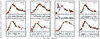 |
Fig. 4. Supernovae parametric model fits and residuals for 8 representative SNe IIb. The red points show the o-band photometry from ATLAS for each of the SNe in our sample. The black continuous line represents each SPM fit. Inside each panel, we indicate the name of the corresponding SN. Bottom Panels display the residuals of the SPM fit for each SN. The dashed lines mark the ±3σr thresholds, which we use to identify outliers. We excluded these outliers from the SPM refitting process. Cyan squares highlight the outliers, which we define as evidence for EE. |
4.1. EE frequency
Using our defined EE detection methodology, we identify a total of 20 EE SNe from the entire sample of 66 SNe IIb analysed by applying the criterion defined in Section 3.1, without considering additional criteria for explosion epoch error (δtexp) or observational point density (ρpeak). The light curves of these 20 SNe, normalised by their main peak flux, are shown in Figure 5.
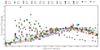 |
Fig. 5. Normalised light curves of the 20 EE SNe. The flux is normalised by the main peak flux in the o-band, illustrating the variability and timing of the EE among the sample. |
We proceeded to quantify the frequency of EE SNe under different criteria for δtexp and ρpeak. Specifically, we consider thresholds for the explosion epoch error δtTH ∈ [1, 2, …, 6] days, and for the observational point density ![Mathematical equation: $ \rho^{\mathrm{peak}}_{\mathrm{TH}} \in [0.0, 0.1, \ldots, 0.4] $](/articles/aa/full_html/2025/09/aa54370-25/aa54370-25-eq10.gif) observations per day, and we apply these thresholds to the sample. Figure 6 illustrates the percentage of SNe IIb exhibiting early flux excess, which ranges from 31.8% to 55.6%, depending on the criteria applied for δtexp and ρpeak. As expected, the frequency of EE SNe increases consistently for smaller explosion epoch errors and higher observational point densities.
observations per day, and we apply these thresholds to the sample. Figure 6 illustrates the percentage of SNe IIb exhibiting early flux excess, which ranges from 31.8% to 55.6%, depending on the criteria applied for δtexp and ρpeak. As expected, the frequency of EE SNe increases consistently for smaller explosion epoch errors and higher observational point densities.
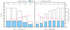 |
Fig. 6. Supernovae counts and EE percentages under specific criteria. The number of SNe IIb satisfying specific criteria for observational point density (ρpeak > ρTH, left panel) and explosion epoch error (δtexp < δtTH, right panel) are shown as unfilled bars. Blue-filled bars represent the subset EE SNe. The dashed pink line indicates the percentage of EE SNe for each criterion, with numerical percentages displayed above the bars. |
4.2. Characterisation of light curve properties
After identifying the 20 EE SNe in the ATLAS sample and calculating their frequency, we characterise their photometric properties in order to compare them with the 46 non-EE SNe.
We characterised the light curve properties using the rise time (trise), the decline rate (ΔM15), and the peak absolute magnitude ( ). The absolute magnitudes were estimated using distances derived from recessional redshifts, assuming a local Hubble-Lemaétre constant H0 = 74.03 ± 1.42 kms−1 Mpc−1 (Riess et al. 2019), with cosmological parameters Ωm = 0.27 and ΩΛ = 0.73, and correcting only for Milky Way extinction from galactic dust reddening reported in Schlafly & Finkbeiner (2011) using ratio of total to selective extinction of RV = 3.1. Host galaxy extinction corrections were not applied because the necessary data are unavailable for all SNe in our sample. Even when such data are accessible for methods such as the colour–colour curve (Rodríguez et al. 2014, 2019), colour evolution (Stritzinger et al. 2018), Balmer decrement (Xiao et al. 2012), or sodium absorption lines (Poznanski et al. 2012), the associated uncertainties in estimating E(B − V) remain significant. As de Jaeger et al. (2018) highlighted, these methods are generally unreliable for SNe II and often introduce additional uncertainties. Furthermore, the poorly constrained RV exacerbates these issues. Consequently, we did not correct for extinction in the host galaxy to avoid adding further uncertainties to our results.
Our analysis was conducted on the 66 SNe IIb sample using different criteria for explosion epoch error (δtexp) and observational point density (ρpeak), as defined in Section 4.1. However, we adopt the subset with ρpeak ≥ 0.3 days−1 (36 SNe: 16 EE and 20 non-EE) as representative, as it offers a good balance between cadence quality and sample size. The explosion epochs are well constrained (median δtexp = 1.4 days), enabling robust statistical analysis. In this subset, we find statistically significant differences in the ΔM15 distributions between EE and non-EE SNe (see Section 4.2.1), and strong correlations between ΔM15 and trise for both groups (see Section 4.2.2). In addition, this subset is representative because their results remain consistent under less restrictive criteria, such as lower density thresholds (ρpeak < 0.2 days−1) and explosion epoch uncertainties δtexp < 4 − 6 days. At the strictest threshold ρpeak > 0.4 days−1, we observe the same trends. However, the smaller sample size (19 SNe: 9 EE and 10 non-EE) limits the statistical significance, particularly in distribution and correlation tests. This drop in significance likely reflects limited data rather than the absence of the underlying correlations.
4.2.1. Distributions of light curve parameters
In this subsection, we compare the light curve properties of EE and non-EE SNe IIb using the Kolmogorov-Smirnov (KS) and Anderson-Darling (AD) tests, focusing on trise, ΔM15, and  . Figure 7 shows the distributions of light curve parameters for EE and non-EE SNe IIb in the representative subset with ρpeak ≥ 0.3 days−1. We find a statistically significant difference in ΔM15 between the two groups, as indicated by the AD test (p = 3.92 × 10⁻²). This difference is consistently observed across a wide range of selection criteria (see Table F.2), including all tested density thresholds below ρpeak < 0.3 days−1 and all explosion time uncertainties δtexp ≤ 6 days. These findings support the robustness of the trend in ΔM15 distributions. At the strictest threshold (ρpeak = 0.4 days−1), a similar result is observed, but it does not reach statistical significance due to the small sample size (19 SNe: 9 EE and 10 non-EE), rather than the disappearance of the underlying difference.
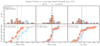 |
Fig. 7. Histograms and cumulative distributions of ΔM15, |

The rise time trise shows marginal differences in some subsets, specifically at ρpeak = 0.0 and 0.1 days−1, and for δtexp = 3 − 4 days. However, as observed in the representative sample (see Figure 7), the 1σ confidence intervals show substantial overlap between EE and non-EE distributions, indicating that the observed differences are not statistically robust. Furthermore, at stricter criteria (ρpeak ≥ 0.3 days−1), the differences in trise disappear altogether. In addition, we find no statistically significant differences in the peak absolute magnitude  distributions between EE and non-EE SNe under any of the selection criteria explored.
In summary, our analysis reveals statistically significant differences between EE and non-EE SNe in the ΔM15 distributions. In contrast, we find similar rise times and peak absolute magnitudes distributions. Table F.2 summarises the complete KS and AD test statistics and p-values across all selection criteria. The implications and qualitative physical interpretation of these results are discussed in Section 5.2.
4.2.2. Correlations in light curve parameters
We investigated possible correlations among light curve parameters in EE and non-EE SNe IIb. We define a statistically significant correlation as having a correlation coefficient ≥ 0.5 and a p-value ≤ 0.05 in either the Pearson or Spearman test.
Figure 8 shows the results for our representative sample (ρpeak ≥ 0.3 days−1). EE SNe exhibit a strong negative correlation between ΔM15 and trise (Pearson r = −0.72, p = 1.66 × 10⁻³), indicating that faster post-peak declining SNe tend to reach maximum brightness earlier. Additionally, we find a significant correlation between trise and  (Pearson r = −0.6, p = 1.28 × 10⁻²), suggesting that brighter SNe reach the peak at early phases. No correlation is found between ΔM15 and
  (r = 0.2, p = 4.55 × 10⁻¹).
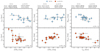 |
Fig. 8. Correlation between ΔM15, trise, and |

Among non-EE SNe, we also observe statistically significant correlations between ΔM15 and trise (r = −0.64, p = 2.03 × 10⁻³), and between trise and  (r = −0.71, p = 3.55 × 10⁻⁴). Additionally, the non-EE sample shows a strong correlation between ΔM15 and
  (r = 0.75, p = 1.22 × 10⁻⁴), suggesting that brighter SNe tend to decline more rapidly after peak.
Table F.1 summarises the correlation coefficients for each observational criterion. In the EE sample, the correlation between ΔM15 and trise and  and trise is consistently observed across all density and explosion epoch error thresholds, suggesting robust correlations.
For non-EE SNe, we find the ΔM15–trise correlation in most criteria, except for ρpeak = 0.4 days−1 (8 SNe) and δtexp = 1 day (7 SNe), where the small sample sizes likely prevent the correlation from reaching statistical significance. In both cases, the data still show a similar trend, suggesting that the lack of significance is more likely due to limited statistical power rather than the absence of an underlying correlation. In contrast, the correlations between  and trise, as well as between ΔM15 and
  , while present in the representative sample, are only recovered at ρpeak = 0.4 days−1, and not consistently under other criteria. In most cases, the correlation strength or significance falls below our defined thresholds (i.e. r < 0.5 and/or p > 0.05), indicating weaker or more dispersed trends. We therefore consider these two correlations in non-EE SNe as not robust.
In summary, we identify a robust and statistically significant correlation between ΔM15 and trise, which persists across all selection criteria for both EE and non-EE SNe. In addition, EE SNe exhibit a significant correlation between Mpeak and trise. In Section 5.1 we discuss these results in more detail.
4.3. Properties of the EE
Motivated by the differences observed in the distributions of light curve parameters between EE and non-EE SNe in Sect. 4.2.1, as well as the correlations identified for EE and non-EE SNe in Sect. 4.2.2, this section aims to characterise the properties of the EE. To achieve this, we first statistically quantify its duration in Section 4.3.1 and subsequently explore differences in colour evolution during the phases where the EE is present, comparing it with the colour of non-EE SNe at similar phases in Section 4.3.2.
4.3.1. Duration of the EE
To statistically characterise the duration of the EE, we estimated an upper limit for its timescale because the low cadence and the limited number of photometric points during the EE do not allow for an accurate estimation. We define this duration as the time interval between the last photometric data point before the EE and the first photometric data point following it, where the residuals fall below the threshold of three residual standard deviations (3σr), as defined in Section 3.2 for identifying the EE. If the point preceding the earliest point satisfying this condition occurs before the explosion epoch, we use the explosion epoch as the first epoch before the EE.
The uncertainty in the upper limit duration of the EE, δtEE, was estimated through error propagation, accounting for the cadence of the light curve and the uncertainty in the explosion epoch when appropriate. Specifically, if the photometric point preceding the first EE point occurs after the estimated explosion time, then 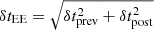 , where δtprev and δtpost correspond to the time gaps between the first and last EE points and their adjacent observations, respectively. Conversely, if the explosion epoch is the only available reference prior to the EE, then
  , where δtexp is the uncertainty in the explosion time. This formulation provides a conservative estimate of the EE duration uncertainty in both scenarios.
For the 20 EE SNe in our sample, the upper limit for the duration of the EE has a mean value of 8.8 days, a median of 8 days, and a standard deviation of 3.7 days. The distribution spans from 3 to 15 days. The uncertainty in this upper limit has a mean value of 4.9, a median of 4.35 days, and a standard deviation of 2.1 days, with values ranging between 2.8 days and 10.3 days.
4.3.2. Colour evolution
After statistically estimating the phases where the EE is present, we study the colour evolution of EE and non-EE SNe during and after these phases. To do this, we used the Zwicky Transient Facility (Bellm et al. 2019) (ZTF) Forced Photometry Service (Masci et al. 2023), which allowed us to download ZTF-g and ZTF-r bands and estimate the g − r colour. We calculated the g − r colour for 59 of the 66 objects in our selected ATLAS sample that the ZTF also observed. The colours were corrected only for extinction in the Milky Way, as described in Section 4.2.
Of the 59 objects, 40 correspond to non-EE SNe and 19 to EE SNe. We focused on comparing the g − r colour of the EE and non-EE SNe. Considering that the median upper limit for the duration of the EE is eight days, we studied the colour before and after this epoch. To analyse the average colour evolution of the EE and non-EE SNe up to phase 30 days after the explosion, we calculated a centred moving average of the g − r colour using consecutive three-day time windows from 0 to 30 days. Each value was assigned to the window’s midpoint, representing the average interval. We computed the mean and standard deviation of the g − r colour measurements for each time window. This approach allowed us to compare the average colour trends between the two groups, particularly before and after eight days post-explosion.
Figure 9 shows the g-r colour evolution for EE and non-EE SNe. During the first three days post-explosion, EE SNe exhibit a mean g − r colour of −0.18 with a standard deviation of 0.4 (based on 10 SNe), while non-EE SNe show a redder mean colour of 0.18 with a smaller dispersion of 0.25 (based on 5 SNe). Although this colour difference is not statistically significant due to the sample size and dispersion, it suggests that EE SNe tend to be intrinsically bluer at early times. Similarity to the literature sample of double-peaked SNe (see Section 4.4.2), further supports this trend.
 |
Fig. 9. Evolution of the g − r colour for EE and non-EE SNe up to 30 days post-explosion. Individual measurements for non-EE SNe are shown as grey points, while pastel-coloured markers represent EE SNe. The solid lines correspond to the centred moving averages, pink for EE and sation for non-EE SNe. Dashed lines indicate the standard deviation (σ) per time bin, and the shaded regions denote the mean ± σ. The vertical black line marks the median upper limit of the EE duration (8 days). |
Between three and six days post-explosion, the mean colours of both groups become more similar, with values of 0.24 ± 0.33 for EE SNe and 0.27 ± 0.41 for non-EE SNe. From six to nine days, EE SNe remain slightly redder on average (0.39 ± 0.29) than non-EE SNe (0.27 ± 0.32), though the difference is modest. Beyond this phase, the colour evolution of both groups converges progressively, with comparable mean values and overlapping dispersions in subsequent intervals up to ∼30 days post-explosion.
4.4. Literature sample with an EE interpreted as shock cooling emission
In this section, after identifying 20 EE-SNe and characterizing their light curves and colours, we investigate whether the EE observed in the ATLAS sample can be attributed to SC emission from the progenitor envelope after shock breakout. To address this, we compare the photometric properties of the ATLAS EE-SNe with those of nine SNe IIb from the literature that exhibit SC emission, aiming to assess their consistency with this physical origin.
The literature sample is characterised by its higher sampling quality than the ATLAS sample. Specifically, the mean observational point density for these SNe in the V band is  , significantly higher than the ATLAS sample’s
  . Similarly, the mean explosion epoch uncertainty for the literature sample is
  days, substantially lower than the ATLAS sample’s
  days.
days.
The improved sampling properties of the literature sample result from the targeted follow-up campaigns conducted for the literature SNe. In contrast, the ATLAS sample is obtained from a survey with a default sky-scanning cadence, resulting in less frequent observations. The superior sampling of the literature sample enables more precise estimates of light curve parameters than the ATLAS sample.
4.4.1. Light curves
To characterise the light curves through ΔM15, trise, and Mpeak, and to further characterise the SC phase using parameters described below, we employed Automated Loess Regression (ALR). ALR is a non-parametric method that fits local polynomials with a smoothing parameter that adjusts the fit to local variations in the curve (Rodríguez et al. 2019). We chose ALR over SPM because the SPM cannot accurately model the main peak of the light curve due to the high number of photometric points during the SC phase and the inability to fully exclude SC photometric points during the iterative refitting process defined in Section 3.2. In this context, ALR provides a more reliable representation of the SC, transitional phase, and main peak.
Figure 10 illustrates the light curves and their interpolations. We estimate the SC duration dSC as the time between the explosion and the minimum flux in the transitional phase (ttrans) between the SC and the main peak. Table 4.4.3 lists the SC literature sample, reporting their explosion epoch, colour excess, SC duration, distance, and their corresponding references. The SC duration has a mean of  days, a median of
  days, and a standard deviation of σdSC = 3.37 days.
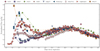 |
Fig. 10. Normalized light curves of nine SNe with SC emission compiled from the literature, presented in different photometric bands. Analogous to Figure 5, the light curves are normalized by the flux of the second peak, illustrating the diversity of SC properties. Solid lines represent the ALR interpolation of the first and second peaks, while the dashed line represents the transition between the two peaks. |
This methodology to estimate the SC duration is not feasible for the ATLAS EE SNe because their lower cadence does not allow for the observation of the transition between the two peaks in most cases. This limitation highlights another reason for investigating the literature sample. Its higher observational quality allows for a more detailed characterisation of the SC phase and its properties.
In addition to the SC duration, we also estimate the absolute magnitude during the transition, Mtrans, and the peak absolute magnitude in the SC as Mpeak, SC. The Mpeak, SC for SNe 2011h, 2016gkg, 2020bio, and 2013df was estimated as a lower limit because the SC peak is not sampled. Therefore, we assume the Mpeak, SC value as the earliest SC photometric point. Additionally, we estimate parameters related to the main peak, such as trise, Mabs5, and ΔM15. All the parameters above were calculated for the six SNe6 with photometry in the V-band, as it provides the largest sample of objects for consistent analysis.
We explored potential correlations between parameters measured during the shock SC phase and those associated with the main peak of the light curve. Correlations were considered significant if at least one of the statistical tests (Pearson, Kendall, or Spearman) had a p-value below 0.05. In this case, all significant correlations also presented a correlation coefficient greater than |r|> 0.82, providing strong evidence of the relations described. The detailed correlation coefficients and p-values for all parameter pairs across these tests are provided in each top panel in Figure 11. Below, we describe the significant correlations observed within the SC phase, the main peak, and between these two phases.
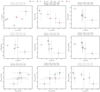 |
Fig. 11. Correlation analysis between parameters measured during the shock SC phase and those associated with the main peak of the light curve for the literature sample. Significant correlations are highlighted, including relationships within the SC phase, such as between the transitional absolute magnitude (Mtrans) and the SC rise time (trise), and between the SC peak absolute magnitude (Mpeak, SC) and Mtrans. Correlations within the main peak include Mpeak and trise. Additionally, correlations between the SC phase and the main peak are shown, including ttrans with trise, Mpeak, SC with trise, and Mpeak, SC with Mpeak. These relationships provide evidence linking the SC phase to the main peak properties, highlighting the continuity of physical processes across both phases. Non-significant correlations are also shown for completeness. |
Within the SC phase, a strong correlation was observed between the transitional absolute magnitude (Mtrans) and the transitional time (ttrans), indicating that prolonged SC phases correspond to brighter transitions. While a trend between the peak SC absolute magnitude (Mpeak, SC) and Mtrans is observed, it is not statistically significant (Pearson: −0.74, p-value: 9.4 × 10⁻²). This suggests that brighter SC peaks may tend to produce brighter transitions; however, a larger sample sise, along with precise measurements instead of upper limits, is needed to confirm or reject this trend.
In the main peak, we identified a correlation between the peak absolute magnitude (Mpeak) and the rise time (trise), where brighter SNe tend to exhibit longer rise times.
Correlations between the SC phase and the main peak reveal further links between the early phases and the peak of the light curve. The peak SC absolute magnitude (Mpeak, SC) was found to correlate with the rise time to the main peak (trise), showing that brighter SC peaks are associated with longer rise times. Additionally, Mpeak, SC correlates with the peak absolute magnitude of the main peak (Mpeak), demonstrating that brighter SC peaks are linked to brighter main peaks. Lastly, while no significant correlation was found between the duration of the SC phase (ttrans) and the rise time to the main peak (trise), a trend is observed where longer SC phases tend to result in later main peaks.
While these significant correlations provide insight into the statistical relation between SC parameters and the main peak, several correlations did not reach statistical significance with the current sample size. For instance, the correlation between ΔM15 and trise showed moderate trends but lacked sufficient statistical strength to draw definitive conclusions. A larger sample is necessary to confirm or reject these correlations.
4.4.2. Colours
In addition to analysing the light curve properties of the SNe with SC from the literature, we studied their optical colour evolution. Among the colours, the B − V colour is the most commonly available, with six SC SNe having the necessary photometry to calculate B − V. As previously mentioned in Section 4.2, the colours were corrected only for extinction in the Milky Way.
To compare the B − V colour of the six SC SNe, we defined a sample of SNE IIb without the presence of the SC (non-SC SNe sample). The non-SC sample consists of seven SNe IIb from the literature with early photometric observations, all at phases earlier than the average SC duration (8.8 days), in which visual inspection suggests the absence of SC in this sample, as no photometric points were consistent with an EE. Of these non-SC SNe, four have data earlier than two days, and three have data earlier than 6.3 days.
The B − V colour evolution for SNe with and without SC is shown in Figure 12. We estimated the average colour using the same methodology described in Section 4.3.2.
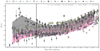 |
Fig. 12. B − V colour evolution for SNe with (seven) and without (five) SC up to 30 days post-explosion. Individual data points for SNe without SC are sation, while pastel-coloured markers represent those with SC. Solid lines show the centred moving averages, with pink representing SNe with SC and sation for those without SC. Dashed lines indicate the standard deviation (σ) around the mean for each time interval, and the filled regions represent the mean ± σ. The vertical black line marks the average upper limit for the SC duration. Analogous to Figure 9, this figure emphasizes the differences in colour evolution between the two groups, particularly in the early phases. |
To analyse the B − V colour evolution during and after the SC phase, we use the average duration of the SC phase (8.8 days) as a reference point. During the first three days after the explosion, SNe with SC exhibit significantly bluer colours (B − V = 0.11 ± 0.14) compared to those without SC (B − V = 0.49 ± 0.24), with the colour difference being statistically significant7. After this period, the colours converge, overlapping within the standard deviation range. Beyond the SC phase (after nine days), the differences between the two groups diminish further. At later phases, such as 18–21 days, the mean B − V colour for SNe with SC is 0.44 ± 0.16, compared to 0.56 ± 0.23 for those without SC, indicating a convergence in colour evolution. However, a larger dataset is necessary to confirm these trends due to the small sample size. These results show that the B − V colour differences between SNe with and without SC are consistent with the trends observed in the ATLAS EE sample. The implications of these findings, along with their relevance to the physical origin of EE in SNe IIb, are discussed in detail in Sect. 4.4.3.
4.4.3. Comparison of EE and shock cooling properties
At this stage, we have identified the EE, characterised its photometric properties, and compared it with non-EE SNe. We next explore its possible origin by comparing it with SNe exhibiting SC emission, as detailed in Section 4.4. We focus on their durations, colour evolution, and correlations among light curve parameters.
In Section 4.3.1, we estimated an upper limit for the EE duration using the ATLAS sample, while Section 4.4.1 provided the SC emission duration from the literature sample. The methodologies differ primarily due to more precise explosion epoch determinations and higher observational densities in the literature sample.
We conducted statistical tests on both samples to compare the durations. The KS and Mann-Whitney U (MWU) tests yield a KS statistic of 0.3 (p-value = 0.61) and a U statistic of 77 (p-value = 0.9), respectively. In both cases, the p-values exceed the conventional threshold of 0.05, indicating that we cannot reject the null hypothesis that the durations of the EE and SC emissions come from the same distribution. These results suggest that the upper limit of the EE duration could be consistent with the duration of the SC emission.
In addition to comparing EE and SC emission durations, we analysed their colour evolution trends. Both features show similar timescales, with EE lasting a median of eight days and SC having a mean duration of 8.8 days. During the SC phase, SNe with SC exhibit statistically significant bluer B − V colours compared to those without SC. Although the dispersion in the data prevents statistical significance, EE SNe show a similar trend, displaying bluer g − r colours than non-EE SNe, particularly at phases earlier than five days. Despite using different filter systems, both EE and SC samples follow a consistent trend of blue colour evolution during the early phases.
We also examined whether the correlations observed in the ATLAS sample (ΔM15–trise and Mpeak–trise) are also present in the SC SNe literature sample. In both samples, the general trends are consistent: SNe with slower post-peak declines (ΔM15) tend to have longer trise, and brighter peak magnitudes (Mpeak) are associated with early phases of trise.
The ATLAS sample shows statistically significant correlations for both pairs under representative criteria (e.g. ρpeak ≥ 0.3 days−1), the literature sample similarly displays a statistical significant strong negative correlation for trise − Mpeak. On the other hand, the relation of trise − ΔM15 shows consistent behaviour with the ATLAS sample, but is not statistically significant, probably due to the reduced sample size (five SNe).
These similarities between the ATLAS sample and the literature suggest that the features we identify as EE in ATLAS SNe could indicate the same physical processes driving SC as described in previous studies.
4.5. Robustness of our results
In this section, we analyse the robustness of our results by removing potential false positives EE SNe and possible peculiar/misclassified objects. We define a criterion for identifying false positives within the EE sample detected in Section 4.1. In addition, we use our defined cleaned sample that excludes the four objects (SN 2019hte, SN 2021iiu, SN 2022fzf, SN 2022W) based on our method in Appendix B.2, identified as possible misclassified/peculiar objects.
After excluding these false positives and using our cleaned sample, we recalculate the observed frequency of SNe with EE in the ATLAS sample in Section 4.5.2. Subsequently, in Section 4.5.3, we examine whether the differences in the distributions of light curve parameters between EE and non-EE SNe, observed for the entire sample in Section 4.2.1, persist. Also, Section 4.5.3 assesses whether the correlations observed for SNe with EE remain consistent after removing the three false positives.
4.5.1. Verification of EE detections
This section assesses the validity of the 20 SNe identified with EE. We specifically examined cases in which our method detected only one photometric point that satisfied the criterion of having a residual, defined as the difference between the observed flux and the SPM, greater than three times the standard deviation of the residuals (3σr), considering it as an EE. Nine of the 20 SNe detected meet this condition in the ATLAS light curves, of which seven have additional g- and r-band photometry from ZTF. We visually inspected these seven ZTF light curves to verify whether photometric points consistent with the single EE point detected in ATLAS were present. As shown in Figure 13, five of these seven objects exhibit flux consistent with the EE detected in ATLAS. However, the remaining two SNe and the two SNe that only have a single point detected in ATLAS and lack ZTF photometry are considered potential false positives.
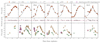 |
Fig. 13. Zwicky Transient Facility verification of potential false positives with ZTF photometry. The top panels show the ATLAS o-band photometry, with potential SC points enclosed by blue open squares. The middle panels illustrate the residuals produced by the SPM model. The bottom panels display the ZTF g- and r-band photometry, with points consistent with an EE identified by visual inspection and enclosed in purple open circles. |
For these four potential false positives, we redefined the criterion for EE detection by adopting a more conservative threshold of eight times the standard deviation of the residuals (8σr) instead of the original 3σr defined in Section 3.2. This threshold was chosen for its highly conservative nature, as such extreme values have a negligible probability (< 10−15) of arising from statistical noise under a normal distribution, significantly reducing the risk of false positives. As a result, only SN 2017ixz satisfies this stricter criterion, while the remaining three objects (SN 2023xoo, SN 2019rn, and SN 2024jcf) were removed from our sample.
4.5.2. Verification of the frequency
In this section, we test the robustness of the EE SNe frequency using our cleaned sample of 59 SNe IIb, and removing objects identified as peculiar or misclassified. Figure 14 shows the new frequency estimation across the different density and explosion epoch thresholds. We analysed variations in the EE frequency across the different thresholds, comparing this result with those obtained in Section 4.1.
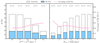 |
Fig. 14. Same as Figure 6 using our defined cleaned sample after rejecting potential false positive EE SNe. |
The representative subsample (ρpeak ≥ 0.3 days−1) shows an EE SNe frequency that decreases from 44.4% when using the full sample to 42.4% when using the cleaned sample and excluding potential false positives. This new estimation is consistent with those obtained from the full sample in Section 4.1, representing a modest reduction of 2%.
We examined density criteria ranging from 0 days−1 to 0.4 days−1 and found that the frequency of SNe with EE varies from 31.8% to 47.4% in the full sample, compared to 30.5% to 44.4% in the new estimation. On the other hand, for the explosion epoch error criteria, the frequency decreases from 31.8% to 55.6% in the full sample to 30.5% to 50% in the new estimation. The frequencies are lower than those of the full sample presented in Section 4.1; however, they remain consistent, with a maximum difference of 5.6%.
4.5.3. Validation of distributions and correlations
Another important aspect is to verify whether the differences in the distributions of light curve parameters between SNe with and without EE observed in the full sample persist using the cleaned sample and removing potential EE false positive SNe. In addition, we verify if the correlations observed in the full sample, such as ΔM15-trise for EE and non-EE SNe and Mpeak-trise for EE SNe, remain consistent in the new estimation.
Figure 15 shows the cumulative distributions of ΔM15, trise, and Mpeak for the cleaned sample after removing potential EE false positives SNe. We find a statistically significant difference in the ΔM15 distributions based on the KS test (0.5, p-value = 1.89 × 10⁻²) as in the full sample. In contrast, Mpeak and trise show no statistically significant differences.
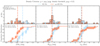 |
Fig. 15. Same as Figure 7, but after removing potential false positives among EE SNe (Section 4.5.1) and possibly misclassified objects (Section 2), reducing the sample from 66 to 59 SNe. |
Table F.2 summarises the KS and AD test results for ΔM15, trise, and Mpeak under all selection criteria. We consistently observe a significant difference in the ΔM15 distribution between EE and non-EE SNe across all criteria. Additionally, Mpeak distributions show no significant differences under any selection criterion. Finally, similar to the full sample, trise shows marginal differences under some criteria (e.g. ρpeak = 0 days−1 and δtexp ≥ 3 days); however, the 1σ confidence regions display substantial overlap between the EE and non-EE distributions (see right panels of Figures 7 and 15), and the difference further vanishes under more restrictive selection criteria.
In summary, these new results lead to the same conclusions discussed in Section 4.2.1, reinforcing the robustness of our findings. We identify statistically significant differences between EE and non-EE SNe in the ΔM15 distributions, while trise and Mpeak remain statistically similar. In addition to corroborating the distributions, we verify the correlations found in our full sample analysis (Section 4.2.2) and obtain consistent results in our cleaned sample.
Figure 16 shows the results for the representative sample (ρpeak ≥ 0.3 days−1), where we identify a statistically significant correlation between ΔM15 and trise for both EE and non-EE SNe, consistent with the results from the full sample. Additionally, we observe a correlation between Mpeak and trise in EE SNe. The same correlation appears in non-EE SNe; however, as discussed below, it weakens under stricter selection criteria.
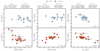 |
Fig. 16. Same as Figure 8, but after removing potential false positives among EE SNe (Section 4.5.1) and possibly misclassified objects (Section 2), reducing the sample from 66 to 59 SNe. |
The correlation between ΔM15 and trise in EE SNe persists across all selection criteria except for the density threshold ρpeak = 0.4 days−1, where the small sample size (8 SNe) results in a non-significant p-value (5.8 × 10⁻²), despite maintaining a correlation coefficient |r|> 0.5. For non-EE SNe, this correlation is also present in all criteria except for ρpeak = 0.4 days−1 (10 SNe) and δtexp = 1 day (7 SNe), where the reduced sample sizes similarly prevent statistical significance. In addition, the correlation between Mpeak and trise in EE SNe holds under all criteria except for δtexp = 1 − 2 days, where the limited number of objects (7 and 10 SNe, respectively) prevents the p-value from reaching significance, even though the correlation strength remains high (|r|> 0.5).
In summary, we confirm the presence of the ΔM15–trise correlation in both EE and non-EE SNe, as well as the Mpeak–trise correlation in EE SNe, supporting the robustness of the results presented in Section 4.2.2.
5. Discussion
5.1. Correlation analysis of light curve parameters
We now qualitatively assess the observed correlations in our sample, focusing on the ΔM15–trise and Mpeak–trise relations, and explore their potential physical origins. We also examine correlations between the SC phase and the main peak based on a literature sample (4.4.1).
Dessart et al. (2016) reported a correlation between ΔM15 and trise, finding a strong relation in their simulations of SESNe (including SNe IIb) that resulted from the terminal explosions of mass donors in close-binary systems. In their model, more massive ejecta lead to longer diffusion timescales, producing slower post-peak declines and later peak times. Similarly, Rodríguez et al. (2023) observed this correlation for SNe Ib and Ic, where faster post-peak decline light curves tend to reach the peak at earlier phases. However, they reported no significant correlation for SNe IIb.
Our analysis reveals a strong correlation between ΔM15 and trise for both EE and non-EE SNe, indicating that fast post-peak declining light curves tend to reach maximum brightness at earlier phases. This behaviour is consistent with the expectation that more massive ejecta produce longer diffusion timescales, resulting in slower declines and later peak times. Additionally, we find a significant correlation between trise and Mpeak for EE SNe. Although this correlation also appears in the representative non-EE subsample, it is not under any other selection criterion, suggesting that non-EE SNe may form a more heterogeneous group compared to EE SNe, which exhibit lower scatter in their photometric properties. Finally, we detect no correlation between ΔM15 and Mpeak for either EE or non-EE SNe. Previous studies, such as Drout et al. (2011), Prentice et al. (2016), and Dessart et al. (2016), have also reported the absence of such a correlation for SESNe, including SNe IIb. The lack of correlation likely arises from the complex and non-uniform relationship between explosion mechanisms and ejecta properties. In particular, Dessart et al. (2016) attributed the wide scatter in both ΔM15 and Mpeak to the fact that the amount of 56Ni synthesised primarily governs the peak absolute magnitude. In contrast, the post-maximum decline rate depends on a combination of 56Ni mass, ejecta mass, and kinetic energy.
In the literature sample, correlations observed between the SC phase and the main peak suggest a link between the energy source driving the SC and the subsequent light curve evolution. The SC peak absolute magnitude (Mpeak, SC) shows significant correlations with both the rise time to the main peak (trise) and the main peak absolute magnitude (Mpeak), highlighting that brighter SC peaks are associated with brighter and slower-evolving main peaks. These findings suggest a shared underlying energy source or mechanism influencing both phases. In addition, a trend between the SC duration (ttrans) and trise shows that SNe with longer SC phases tends to take more time to reach their main peak; however, this correlation is not statistically significant (p-value > 0.05), a larger sample is required to confirm or reject this potential correlation. Given the small sample of six SNe, further data is essential to validate these correlations robustly.
Assuming the previously described correlations exist, no clear hypothesis currently explains this connection. Analytical models suggest that more massive H-rich envelopes produce longer SC phases, while more extended envelopes result in brighter SC peaks. Furthermore, Park et al. (2024) demonstrated that the brightness of the first peak can be reduced by more than a factor of three due to Thomson scattering. If an extended H-rich envelope primarily powers SC, the observed correlations between SC timescales, brightness, and the main peak could indicate that H recombination influences the phases of the main peak. Given the limited sample size and the lack of a comprehensive explanation for these correlations, hydrodynamical studies exploring these relationships under specific physical conditions are necessary.
5.2. Light curve parameter distributions: Qualitative physical interpretation
In this section, we discuss the cumulative distributions of ΔM15, trise, and Mpeak for EE and non-EE SNe, as presented in Section 4.2.1, and explore their physical interpretation in terms of explosion parameters inferred from correlations with these observables. Given that these parameters exhibit similar trends across individual bands and bolometric light curves (Rodríguez et al. 2023), we base our qualitative interpretation on their measurements in the o-band.
Explosion properties such as ejecta mass (Mej), 56Ni mass, and explosion energy (E) have been inferred from analytical modelling of bolometric light curves of SESNe, revealing correlations between these physical parameters and observable light curve properties, including rise and decline rates, characteristic timescales, and peak absolute luminosities (Drout et al. 2011; Lyman et al. 2016; Prentice et al. 2016, 2019; Rodríguez et al. 2023). A well-established correlation exists between 56Ni mass and peak absolute magnitude for SNe IIb (Lyman et al. 2016; Prentice et al. 2016), consistent with expectations from the Arnett-rule model for SNe Ia (Arnett 1982), where the decay of 56Ni powers the light curve (MNi ∝ Lp). However, this model is inaccurate for SESNe, as their diffusion time (tdiff) is comparable to the dynamical timescale (tdyn), leading to adiabatic losses during ejecta expansion. As a consequence, the Arnett rule tends to overestimates 56Ni mass by a factor of ∼2 compared to values derived from luminosity measurements during the radioactive tail phase (e.g. Meza & Anderson 2020). At phases later than ∼60 days post-explosion, the ejecta becomes optically thin (tdiff ≪ tdyn), and the luminosity directly traces the energy deposition of 56Ni decay. Using this method, Rodríguez et al. (2023) also reported a strong correlation between 56Ni mass and peak absolute magnitude for SNe IIb.
The similarity in the cumulative distributions of peak absolute magnitude between EE and non-EE SNe suggests that their 56Ni mass distributions are comparable. Since 56Ni production is linked to explosion properties and progenitor core structure (Suwa et al. 2019), this implies that EE and non-EE SNe likely share similar progenitor characteristics. Moreover, explosion models predict that 56Ni mass increases with ZAMS mass (see Figure 14 in Burrows et al. 2024), further reinforcing the idea that both samples originate from progenitors with comparable initial masses.
Rodríguez et al. (2023) identified a correlation between Mej, time to peak tpeak, and post-peak decline ΔM15, based on an analytical framework derived from Arnett’s model (Wheeler et al. 2015). Their results suggest that SNe with more massive ejecta exhibit slower post-peak declines and reach the main peak at later phases, as more massive ejecta leads to longer diffusion timescales. Given the correlation between Mej and ΔM15 (rp = 0.5, p-value < 0.03) reported in Rodríguez et al. (2023) and the statistically higher values of ΔM15 in EE SNe compared to non-EE SNe, this suggest that EE SNe likely have lower ejecta masses. On the other hand, considering the correlation between Mej and tpeak (rp = 0.65, p-value < 0.03) reported by Rodríguez et al. (2023), and the similarity in the tpeak distributions for EE and non-EE SNe, we infer that the ejecta masses are likely comparable between both groups. The discrepancy between the ejecta masses (Mej) inferred from the ΔM15 and trise distributions may arise from several reasons. First, these correlations are based on Arnett’s model, which is not strictly valid for SESNe and thus not fully applicable to SNe IIb. If ejecta mass estimates derived from Arnett’s formalism are assumed to be valid for SNe IIb, the correlation between trise and Mej appears stronger than that between ΔM15 and Mej (Rodríguez et al. 2023), suggesting that EE and non-EE SNe likely have similar ejecta masses. On the other hand, the post-peak decline is primarily governed by a combination of 56Ni mass, ejecta mass, and kinetic energy (Dessart et al. 2016). Given that the 56Ni mass inferred from the peak absolute magnitude is comparable for both groups, we attribute the observed differences in ΔM15 distributions between EE and non-EE SNe to variations in ejecta mass and/or kinetic energy. Additionally, given the similarities in duration and colour between EE and SC SNe, and considering that the conditions required to produce SC are associated with extended envelopes, it is reasonable to expect that such structures could influence parameters such as ΔM15. However, confirming this hypothesis would require, for example, hydrodynamical simulations of SN explosions from progenitors with envelopes of similar mass but different degrees of extension.
In summary, without relying on a specific model, the observed differences in the ΔM15 distributions between EE and non-EE SNe may indicate intrinsic differences in their ejecta properties. Moreover, the similarity in the Mpeak distributions for EE and non-EE SNe implies a similar amount of synthesised 56Ni, based on the empirical correlation between Mpeak and 56Ni mass, which is independent of Arnett’s model. The previous analysis leads to a natural question: how do the progenitors of EE SNe attain these properties if they are otherwise similar to non-EE SNe?
5.3. Implications for the progenitor systems
Motivated by the similarities in colour and duration between EE and SC features discussed in Section 4.4.3, as well as the differences in ejecta properties between EE and non-EE SNe inferred from the ΔM15 distributions, we qualitatively constrain the progenitor systems by considering the ejecta conditions required to produce SC emission, as suggested by analytical and numerical models.
Alternative hypotheses have been proposed to explain the SC feature, such as circumstellar material (CSM) interaction; however, observational evidence has revealed inconsistencies. For instance, SN IIb 2013cu exhibited flash-ionised spectral features approximately 15 hours after explosion, providing clear evidence of CSM interaction, but showing a single-peaked light curve (Gal-Yam et al. 2014). Additionally, all eleven SNe IIb with reported SC emission in the literature have interpreted this feature as originating from the SC of an extended envelope.
Assuming that the EE observed in the EE SNe identified in this study originates from SC emission, we explore scenarios that could lead to different envelope properties, such as extended versus compact envelopes. It is difficult to explain the difference in the progenitor envelope under the assumption of a single progenitor channel, in which the mechanism responsible for stripping the envelope should be similar for similar progenitors. In this context, the most plausible explanation involves binary progenitor systems. Observational and theoretical evidence strongly support the hypothesis that the progenitors of SNe IIb are binary systems (e.g. Claeys et al. 2011; Yoon et al. 2017; Sravan et al. 2019, 2020).
The models presented by Dessart et al. (2024) are particularly illustrative in the context of our results. These models assume the same initial progenitor, with fixed 56Ni mass and explosion energy, and demonstrate how varying the initial binary period leads to different evolutionary outcomes and envelope properties (e.g. ejecta extension and hydrogen mass), ultimately producing double-peaked light curves. However, these models aim to reproduce the entire diversity of core-collapse SNe (i.e. SNe Ic → Ib → IIb → II-L → II-P), rather than focusing specifically on the diversity within SNe IIb. Dedicated hydrodynamical modelling of the light curves of EE and non-EE SNe IIb is required to test whether the observed differences in ΔM15 and similarities in trise can be consistently reproduced.
In summary, we propose that the 20 EE SNe identified in this study originate from SC emission produced by an extended envelope. In addition, both groups’ progenitors are similar, where binary interactions lead to compact/extended envelopes producing non-EE and EE SNe.
6. Conclusions
In this study, we developed a methodology to reclassify SNe IIb reported in the TNS and to identify potentially misclassified or peculiar cases. We also introduced a method to identify EE SNe IIb, which we applied to the ATLAS survey, leading to the detection of 20 EE SNe. We quantified the frequency of EE SNe IIb under specific light curve sampling conditions, inferring a range between 30.5% and 50%.
The 20 EE SNe identified in this study exhibit durations and colour-evolution trends consistent with SNe IIb showing SC emission reported in the literature, suggesting that their origin may be related to progenitors with extended envelopes. Furthermore, the EE SNe in the ATLAS sample display distinct photometric properties compared to non-EE SNe, including statistically significant differences in ΔM15, while showing similar values of Mpeak and trise. These findings suggest that EE and non-EE SNe IIb may originate from progenitors with comparable initial properties but distinct ejecta structures. In this context, binary interactions provide a more plausible explanation for the observed diversity than single-star evolution. Our results constrain the fraction of massive stars that retain the envelope configurations required to produce SC emission. Population synthesis models aiming to reproduce the observed properties of SNe IIb progenitors and their explosions should account for the frequency of EE SNe and the physical conditions required to generate the envelope structures responsible for their early-time emission. Thus, EE SNe provide a valuable observational probe for testing and refining models of stellar evolution and binary interaction.
This study represents a starting point in several respects. First, as discussed in Section 2, the possible presence of SNe II or Ib misclassified as IIb in the TNS sample implies that the reported EE frequency should be considered a lower limit, potentially introducing a bias in our results. Resolving this issue will require a comprehensive analysis of the full CCSNe sample observed by ATLAS in future work. Second, a systematic study using hydrodynamical models of light curves from pre-SN progenitors shaped by binary interactions is needed to test whether the observed differences in ΔM15 and trise can be reproduced, thereby confirming or challenging the interpretations proposed in this work and helping to constrain the evolutionary pathways of SNe IIb progenitor systems.
Period around new moon when the night sky is darkest, optimal for observing faint astronomical objects.
Here, a photometric data point refers to the result after applying the ATClean procedure described in Appendix A, where the four ATLAS observations per night are combined into a single measurement.
Redshift values were obtained from the host galaxy using the NASA/IPAC Extragalactic Database (NED; Helou et al. 1991) when available; otherwise, the value reported in TNS was used.

The ΔM15 value for SN 2016gkg is not available due to the lack of V-band photometry 15 days after the second peak.
Statistically significant indicates that the differences exceed one standard deviation 1σ.
SNID provides a list of template matches, typically reporting how many templates yield rlap ≥ 5.
GELATO always returns the 20 best-matching templates regardless of quality.
Therefore, we cleaned the light curves of these SNe II and estimated their explosion epochs using the same methodology as for the SNe IIb sample.
ΔM30 is calculated analogously to ΔM15, as the difference in magnitude between the peak and 30 days after the peak.
Acknowledgments
We thank Luc Dessart and the anonymous referee for their insightful comments and suggestions, which helped to improve the paper. This research was funded in whole or in part by National Science Centre, Poland, through the PRELUDIUM grant 2024/53/N/ST9/00350. BA acknowledges support from National Agency for Research and Development (ANID) grants ANID-PFCHA/Doctorado Nacional/21221964. MR acknowledges support from National Agency for Research and Development (ANID) grants ANID-PFCHA/Doctorado Nacional/2020-21202606. RD acknowledges funds by ANID grant FONDECYT Postdoctorado N° 3220449. FF acknowledges support from Centro de Modelamiento Matemático (CMM) BASAL fund FB210005 for center of excellence from ANID-Chile. SJS acknowledges funding from STFC Grants ST/Y001605/1, ST/X006506/1, ST/T000198/1, a Royal Society Research Professorship, and the Hintze Charitable Foundation. This work was funded by ANID, Millennium Science Initiative, ICN12_009. MS is a scholarship holder of the Adam Mickiewicz University Foundation in Poznan for the academic year 2024/2025.
References
- Arcavi, I., Gal-Yam, A., Yaron, O., et al. 2011, ApJ, 742, L18 [Google Scholar]
- Arcavi, I., Hosseinzadeh, G., Brown, P. J., et al. 2017, ApJ, 837, L2 [NASA ADS] [CrossRef] [Google Scholar]
- Armstrong, P., Tucker, B. E., Rest, A., et al. 2021, MNRAS, 507, 3125 [Google Scholar]
- Arnett, W. D. 1982, ApJ, 253, 785 [Google Scholar]
- Bellm, E. C., Kulkarni, S. R., Graham, M. J., et al. 2019, PASP, 131, 018002 [Google Scholar]
- Benvenuto, O. G., Bersten, M. C., & Nomoto, K. 2013, ApJ, 762, 74 [NASA ADS] [CrossRef] [Google Scholar]
- Bersten, M. C., Benvenuto, O. G., Nomoto, K., et al. 2012, ApJ, 757, 31 [Google Scholar]
- Bersten, M. C., Folatelli, G., García, F., et al. 2018, Nature, 554, 497 [Google Scholar]
- Blondin, S., & Tonry, J. L. 2007, ApJ, 666, 1024 [NASA ADS] [CrossRef] [Google Scholar]
- Bufano, F., Pignata, G., Bersten, M., et al. 2014, MNRAS, 439, 1807 [Google Scholar]
- Burrows, A., Wang, T., & Vartanyan, D. 2024, ApJ, 964, L16 [NASA ADS] [CrossRef] [Google Scholar]
- Claeys, J. S. W., de Mink, S. E., Pols, O. R., Eldridge, J. J., & Baes, M. 2011, A&A, 528, A131 [NASA ADS] [CrossRef] [EDP Sciences] [Google Scholar]
- Clocchiatti, A., Wheeler, J. C., Benetti, S., & Frueh, M. 1996, ApJ, 459, 547 [Google Scholar]
- de Jaeger, T., Anderson, J. P., Galbany, L., et al. 2018, MNRAS, 476, 4592 [NASA ADS] [CrossRef] [Google Scholar]
- Dessart, L., Hillier, D. J., Woosley, S., et al. 2016, MNRAS, 458, 1618 [NASA ADS] [CrossRef] [Google Scholar]
- Dessart, L., Yoon, S.-C., Livne, E., & Waldman, R. 2018, A&A, 612, A61 [NASA ADS] [CrossRef] [EDP Sciences] [Google Scholar]
- Dessart, L., Gutiérrez, C. P., Ercolino, A., Jin, H., & Langer, N. 2024, A&A, 685, A169 [NASA ADS] [CrossRef] [EDP Sciences] [Google Scholar]
- Drout, M. R., Soderberg, A. M., Gal-Yam, A., et al. 2011, ApJ, 741, 97 [NASA ADS] [CrossRef] [Google Scholar]
- Filippenko, A. V. 1997, ARA&A, 35, 309 [NASA ADS] [CrossRef] [Google Scholar]
- Filippenko, A. V., Matheson, T., & Ho, L. C. 1993, ApJ, 415, L103 [NASA ADS] [CrossRef] [Google Scholar]
- Folatelli, G., Bersten, M. C., Benvenuto, O. G., et al. 2014, ApJ, 793, L22 [NASA ADS] [CrossRef] [Google Scholar]
- Folatelli, G., Bersten, M. C., Kuncarayakti, H., et al. 2015, ApJ, 811, 147 [Google Scholar]
- Foreman-Mackey, D., Hogg, D. W., Lang, D., & Goodman, J. 2013, PASP, 125, 306 [Google Scholar]
- Fremling, C., Ko, H., Dugas, A., et al. 2019, ApJ, 878, L5 [NASA ADS] [CrossRef] [Google Scholar]
- Gal-Yam, A., Arcavi, I., Ofek, E. O., et al. 2014, Nature, 509, 471 [CrossRef] [Google Scholar]
- Georgy, C. 2012, A&A, 538, L8 [NASA ADS] [CrossRef] [EDP Sciences] [Google Scholar]
- Gilkis, A., & Arcavi, I. 2022, MNRAS, 511, 691 [NASA ADS] [CrossRef] [Google Scholar]
- Harutyunyan, A. H., Pfahler, P., Pastorello, A., et al. 2008, A&A, 488, 383 [NASA ADS] [CrossRef] [EDP Sciences] [Google Scholar]
- Heger, A., Fryer, C. L., Woosley, S. E., Langer, N., & Hartmann, D. H. 2003, ApJ, 591, 288 [CrossRef] [Google Scholar]
- Helou, G., Madore, B. F., Schmitz, M., et al. 1991, in Databases and On-line Data in Astronomy, eds. M. A. Albrecht, & D. Egret, Astrophysics and Space Science Library, 171, 89 [NASA ADS] [CrossRef] [Google Scholar]
- Kumar, B., Pandey, S. B., Sahu, D. K., et al. 2013, MNRAS, 431, 308 [NASA ADS] [CrossRef] [Google Scholar]
- Lyman, J. D., Bersier, D., James, P. A., et al. 2016, MNRAS, 457, 328 [Google Scholar]
- Masci, F. J., Laher, R. R., Rusholme, B., et al. 2023, arXiv e-prints [arXiv:2305.16279] [Google Scholar]
- Maund, J. R., Smartt, S. J., Kudritzki, R. P., Podsiadlowski, P., & Gilmore, G. F. 2004, Nature, 427, 129 [NASA ADS] [CrossRef] [Google Scholar]
- Meza, N., & Anderson, J. P. 2020, A&A, 641, A177 [NASA ADS] [CrossRef] [EDP Sciences] [Google Scholar]
- Morales-Garoffolo, A., Elias-Rosa, N., Benetti, S., et al. 2014, MNRAS, 445, 1647 [Google Scholar]
- Nakar, E., & Piro, A. L. 2014, ApJ, 788, 193 [NASA ADS] [CrossRef] [Google Scholar]
- Orellana, M., & Bersten, M. C. 2022, A&A, 667, A92 [NASA ADS] [CrossRef] [EDP Sciences] [Google Scholar]
- Ouchi, R., & Maeda, K. 2017, ApJ, 840, 90 [NASA ADS] [CrossRef] [Google Scholar]
- Park, S. H., Yoon, S.-C., & Blinnikov, S. 2024, ApJ, 960, 63 [NASA ADS] [CrossRef] [Google Scholar]
- Pellegrino, C., Hiramatsu, D., Arcavi, I., et al. 2023, ApJ, 954, 35 [Google Scholar]
- Pessi, P. J., Folatelli, G., Anderson, J. P., et al. 2019, MNRAS, 488, 4239 [NASA ADS] [CrossRef] [Google Scholar]
- Piro, A. L. 2015, ApJ, 808, L51 [NASA ADS] [CrossRef] [Google Scholar]
- Piro, A. L., Haynie, A., & Yao, Y. 2021, ApJ, 909, 209 [NASA ADS] [CrossRef] [Google Scholar]
- Poznanski, D., Prochaska, J. X., & Bloom, J. S. 2012, MNRAS, 426, 1465 [Google Scholar]
- Prentice, S. J., Mazzali, P. A., Pian, E., et al. 2016, MNRAS, 458, 2973 [NASA ADS] [CrossRef] [Google Scholar]
- Prentice, S. J., Ashall, C., James, P. A., et al. 2019, MNRAS, 485, 1559 [NASA ADS] [CrossRef] [Google Scholar]
- Puls, J., Vink, J. S., & Najarro, F. 2008, A&ARv, 16, 209 [NASA ADS] [CrossRef] [Google Scholar]
- Rest, S., Rest, A., Wang, Q., et al. 2023, https://doi.org/10.5281/zenodo.7897346 [Google Scholar]
- Rest, S., Rest, A., Kilpatrick, C. D., et al. 2025, ApJ, 979, 114 [Google Scholar]
- Richmond, M. W., Treffers, R. R., Filippenko, A. V., et al. 1994, AJ, 107, 1022 [Google Scholar]
- Riess, A. G., Casertano, S., Yuan, W., Macri, L. M., & Scolnic, D. 2019, ApJ, 876, 85 [Google Scholar]
- Rodríguez, Ó., Clocchiatti, A., & Hamuy, M. 2014, AJ, 148, 107 [CrossRef] [Google Scholar]
- Rodríguez, Ó., Pignata, G., Hamuy, M., et al. 2019, MNRAS, 483, 5459 [CrossRef] [Google Scholar]
- Rodríguez, Ó., Maoz, D., & Nakar, E. 2023, ApJ, 955, 71 [CrossRef] [Google Scholar]
- Rodríguez, Ó., Nakar, E., & Maoz, D. 2024, Nature, 628, 733 [Google Scholar]
- Ryder, S. D., Van Dyk, S. D., Fox, O. D., et al. 2018, ApJ, 856, 83 [NASA ADS] [CrossRef] [Google Scholar]
- Sana, H., de Mink, S. E., de Koter, A., et al. 2012, Science, 337, 444 [Google Scholar]
- Sánchez-Sáez, P., Reyes, I., Valenzuela, C., et al. 2021, AJ, 161, 141 [CrossRef] [Google Scholar]
- Sapir, N., & Waxman, E. 2017, ApJ, 838, 130 [NASA ADS] [CrossRef] [Google Scholar]
- Schlafly, E. F., & Finkbeiner, D. P. 2011, ApJ, 737, 103 [Google Scholar]
- Schlegel, D. J., Finkbeiner, D. P., & Davis, M. 1998, ApJ, 500, 525 [Google Scholar]
- Shingles, L., Smith, K. W., Young, D. R., et al. 2021, TNSAN, 7, 1 [NASA ADS] [Google Scholar]
- Smartt, S. J. 2009, ARA&A, 47, 63 [NASA ADS] [CrossRef] [Google Scholar]
- Smith, N., & Owocki, S. P. 2006, ApJ, 645, L45 [NASA ADS] [CrossRef] [Google Scholar]
- Smith, N., Li, W., Filippenko, A. V., & Chornock, R. 2011, MNRAS, 412, 1522 [NASA ADS] [CrossRef] [Google Scholar]
- Smith, K. W., Smartt, S. J., Young, D. R., et al. 2020, PASP, 132, 085002 [Google Scholar]
- Soderberg, A. M., Margutti, R., Zauderer, B. A., et al. 2012, ApJ, 752, 78 [NASA ADS] [CrossRef] [Google Scholar]
- Sravan, N., Marchant, P., & Kalogera, V. 2019, ApJ, 885, 130 [NASA ADS] [CrossRef] [Google Scholar]
- Sravan, N., Marchant, P., Kalogera, V., Milisavljevic, D., & Margutti, R. 2020, ApJ, 903, 70 [NASA ADS] [CrossRef] [Google Scholar]
- Srivastav, S., Fulton, M., Smartt, S. J., et al. 2022, TNSAN, 248, 1 [Google Scholar]
- Stritzinger, M. D., Taddia, F., Burns, C. R., et al. 2018, A&A, 609, A135 [NASA ADS] [CrossRef] [EDP Sciences] [Google Scholar]
- Subrayan, B. M., Sand, D. J., Bostroem, K. A., et al. 2025, ApJL, submitted [arXiv:2505.02908] [Google Scholar]
- Suwa, Y., Tominaga, N., & Maeda, K. 2019, MNRAS, 483, 3607 [Google Scholar]
- Taddia, F., Sollerman, J., Leloudas, G., et al. 2015, A&A, 574, A60 [NASA ADS] [CrossRef] [EDP Sciences] [Google Scholar]
- Taddia, F., Stritzinger, M. D., Bersten, M., et al. 2018, A&A, 609, A136 [NASA ADS] [CrossRef] [EDP Sciences] [Google Scholar]
- Takáts, K., & Vinkó, J. 2006, MNRAS, 372, 1735 [CrossRef] [Google Scholar]
- Tartaglia, L., Fraser, M., Sand, D. J., et al. 2017, ApJ, 836, L12 [NASA ADS] [CrossRef] [Google Scholar]
- Tonry, J. L., Denneau, L., Heinze, A. N., et al. 2018, PASP, 130, 064505 [Google Scholar]
- Tully, R. B., Rizzi, L., Shaya, E. J., et al. 2009, AJ, 138, 323 [NASA ADS] [CrossRef] [Google Scholar]
- Van Dyk, S. D., Zheng, W., Fox, O. D., et al. 2014, AJ, 147, 37 [Google Scholar]
- Villar, V. A., Berger, E., Miller, G., et al. 2019, ApJ, 884, 83 [NASA ADS] [CrossRef] [Google Scholar]
- Wang, Q., Armstrong, P., Zenati, Y., et al. 2023, ApJ, 943, L15 [Google Scholar]
- Wheeler, J. C., Johnson, V., & Clocchiatti, A. 2015, MNRAS, 450, 1295 [Google Scholar]
- Woosley, S. E., Eastman, R. G., Weaver, T. A., & Pinto, P. A. 1994, ApJ, 429, 300 [NASA ADS] [CrossRef] [Google Scholar]
- Xiao, T., Wang, T., Wang, H., et al. 2012, MNRAS, 421, 486 [NASA ADS] [Google Scholar]
- Yoon, S.-C., Dessart, L., & Clocchiatti, A. 2017, ApJ, 840, 10 [NASA ADS] [CrossRef] [Google Scholar]
Appendix A: ATClean methodology and parameters
This appendix presents the methodology and criteria implemented in the ATClean tool to process and clean forced photometry data. The procedure identifies and rejects unreliable measurements, incorporates systematic noise estimates, and ensures consistent photometric quality across the light curves. Below, we outline the main steps of the algorithm and the specific thresholds applied during the data cleaning process.
-
For each SN measurement, ATClean constructs eight Control Light Curves (CLCs) by performing forced photometry within a 17″ circular aperture centred near the SN position. These CLCs are empirical references to assess the background noise and systematic uncertainties near the SN.
-
From each CLC, ATClean computes the median flux uncertainty,
 , and the standard deviation of the flux, σf, after applying 3-σ clipping. These values characterise the expected photometric scatter under normal sky conditions.
 -
To identify additional noise contributions not captured by the reported flux uncertainties, ATClean compares σf with
 . If
. If  , an extra noise component is estimated as
  . This extra noise is added in quadrature to the SN flux uncertainties only if the total flux scatter increases by more than 10%, i.e. if
 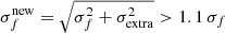 .
. -
The reliability of each SN photometric measurement is evaluated using the expected flux-to-error ratio f/δf ≈ 1 in the CLCs. Deviations from this expectation may indicate observational issues. Therefore, ATClean computes the χCLC2 from a constant-flux model fit to each CLC. A measurement is flagged and discarded if χCLC2 > 2.5, if more than four CLC points are clipped, or if fewer than two remain for averaging.
-
Additionally, ATClean rejects SN measurements with poor photometric quality, specifically when the PSF fit yields χPSF2 > 5 or when the flux uncertainty exceeds 160 μJy, a threshold associated with bright stars near CCD saturation.
-
Corrections are applied for any systematic flux discontinuities arising from periodic updates to the ATLAS reference templates used in image subtraction.
-
Finally, ATClean performs an additional quality control on the SN epochs. It computes the χSN2 from a constant-flux fit after 3-σ clipping. We reject the epoch if χSN2 > 4, if fewer than two measurements remain, or if more than one is clipped.
-
After all corrections and quality checks, the four individual exposures per epoch are averaged. Only exposures passing the PSF χ2 cut, having acceptable uncertainties, and not flagged by the clipping procedure are included in the average.
Appendix B: SN classification
Motivated by the fact that the spectral classification reported in the TNS is not always reliable, we developed a method to classify the SNe spectroscopically (Section B.1) and to identify objects with photometric evolution that deviates from that of typical SNe IIb (Section B.2).
B.1. Spectral classification
We used Supernova Identification (SNID; Blondin & Tonry 2007) and generic classification tool (GELATO; Harutyunyan et al. 2008) to classify the 74 SNe in our sample spectroscopically. We downloaded the available spectra for these objects from the Weizmann Interactive Supernova Data Repository8 (WISEREP). Most have a single classification spectrum. Table B.2 lists the SNe along with the phase of their corresponding classification spectrum. SNID and Gelato determine the best-fit template by comparing the spectrum to be classified to a library of spectra templates.
SNID performs a cross-correlation in logarithmic wavelength space to estimate the SN type, redshift, and phase. SNID quantifies the quality of the match through the rlap parameter, defined as the product of the correlation peak height-to-noise ratio (r) and the logarithmic wavelength overlap (lap). Values of rlap ≳ 5 are typically considered reliable9. GELATO, on the contrary, computes weighted residuals across predefined spectral windows and returns a quality parameter QoF (Quality of Fit), where QoF ≳ 1.5 indicates an acceptable match10.
Table B.1 summarises the number of SNe and spectra of different SESNe in SNID and GELATO, respectively.
Number of SNe and spectra per SN type in the SNID and GELATO template libraries.
To estimate the best match, we forced the redshift using the value of the host galaxy when available in the NASA/IPAC Extragalactic Database (NED; Helou et al. 1991). If the host galaxy redshift was unavailable, we used the redshift reported in TNS. A limitation of both SNID and GELATO is that they do not consider the phase of the input spectrum during the classification process.
Figure B.1 shows an example of the spectral match in SN 2022yep. The best match reported by SNID is SN II-P 2006bp at a phase of +65 days after peak, while the spectrum of SN 2022yep corresponds to +32 days post-peak. Figure B.2 displays the light curve of SN 2022ytx, which shows a post-peak evolution inconsistent with the plateau behaviour of Type II-P SNe, suggesting that SNID’s classification is unreliable in this case.
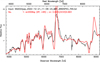 |
Fig. B.1. Supernova Identification best template match of SN 2022yep (black line) with SN 2006bp (red line). The phase of each spectrum relative to the light curve peak is indicated in the figure. |
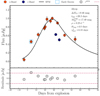 |
Fig. B.2. ATLAS o-band light curve of SN 2022yep. The continuous black line shows the fit using the SPM. Red and blue dots correspond to the photometry in the o and c ATLAS bands, respectively. The bottom panel shows the residuals of the SPM fit, with dashed lines indicating the ±3σr range. |
Motivated by these issues, we defined a method to identify the best template match that combines the classification statistic (either rlap or QoF) with the temporal proximity between the spectrum to be classified and the template. The phase of the spectrum to be classified is well constrained, with an average explosion epoch uncertainty of 2.38 days across our sample.
We defined a score as follows
 (B.1)
(B.1)

where phasestbc is the phase of the spectrum to be classified, and phasetemp is the phase of each template. The variable stat refers to QoF for GELATO and rlap for SNID. We adopt α = 0.4, giving more weight to the statistical quality of the match, while still accounting for the phase information. The score is computed for each template satisfying the quality thresholds (i.e. rlap ≥ 5 or QoF ≥ 1.5). The final classification is assigned based on the individual template (from either SNID or GELATO) that yields the highest score. Given that SNID includes more SNE IIb and spectral templates, we primarily rely on it. GELATO, although useful, has practical limitations: it operates through a web interface, requires 5–7 seconds per object, and returns output only on screen, which must be saved manually. However, we used GELATO instead of SNID in two specific cases:
-
When the redshift estimated by SNID differs from the input redshift by more than 0.020. i.e. |zSNID − zinput|> 0.020.
-
When the best SNID match corresponds to a non-SN source (e.g. AGNs).
Table B.2 presents the best matches based on our score definition. As a result, we classified 67 out of 74 objects as SNe IIb.
Spectral classification results using SNID and GELATO.
B.2. Identifying misclassified or peculiar SNe IIb candidates
To identify objects exhibiting photometric behaviour inconsistent with typical SNe IIb, which could indicate either misclassification or peculiar nature, we analysed their light curve parameters, specifically the post-peak decline and rise time. After the spectral reclassification described in the previous section, the primary potential source of contamination in our final sample of 67 SNe IIb arises from SNe II being misclassified as IIb due to early-phase spectra or peculiar objects.
Therefore, we compiled an initial sample of 92 transients reported as Type II SNe in the TNS and observed by ATLAS. From this set, we selected a subsample of 53 objects with an estimated explosion epoch uncertainty smaller than 6 days—the same threshold applied to our initial sample of 74 SNe IIb. 11
Figures B.3 and B.4 show the light curves of the 53 SNe II and their corresponding SPM fits, which we used to measure key light curve parameters for further comparison with the SNe IIb sample.
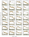 |
Fig. B.3. Supernovae parametric model fits and residuals for 27 SNe II. Orange circles show the ATLAS o-band photometry for each SN. Solid black lines represent the corresponding SPM fits. The name of each SN is indicated in the upper right corner of each light curve panel. Bottom panels display the residuals between the photometry and the SPM fits. The shaded green area marks the ±3σr region, and dashed orange lines indicate the ±3σr thresholds. |
We use the different light curve morphologies between SNe II and SNe IIb (e.g. Pessi et al. 2019) to distinguish between them. We quantified the post-peak decline using both ΔM15 and ΔM30,12 and found that the difference between SNe IIb and SNe II is more pronounced when using ΔM30, as indicated by the KS statistic and its associated p-value: 0.751, p = 3.27 × 10⁻¹⁶ for ΔM15, and 0.802, p = 1.41 × 10⁻¹⁸ for ΔM30.
It is important to note that the SNe II reported in TNS may also be unreliable; for instance, some SNe IIb may have been classified as SNe II (see Section B.2.2). To reduce contamination from peculiar or misclassified objects, we applied a sigma-clipping procedure to the distributions of ΔM30 and trise, removing outliers such as potentially misclassified or peculiar SNe. This process excluded four SNe II from the sample (e.g. SN1987A-like events; see Figure B.5). Therefore, given the sigma clipping and the remaining sample size of 49 objects, we expect the overall trends to remain robust and representative of the SNe II population. In addition, using the same sigma clipping procedure, we removed one object from our sample of 67 SNe IIb: SN 2022ytx, which we briefly discuss in Section B.2.1.
Figure B.5 shows SNe IIb and SNe II in the ΔM30–trise parameter space. SNe IIb exhibit a correlation, as indicated by the Pearson correlation test (r = −0.68, p = 3.45 × 10⁻¹⁰), in contrast to SNe II, which do not show a significant trend. This distinction allowed us to separate the two populations. The figure also marks the spectroscopically rejected objects discussed in the previous section and those removed through the sigma-clipping procedure.
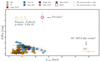 |
Fig. B.5. SNe IIb (blue dots) and SNe II (orange dots) in the trise–ΔM30 parameter space. Objects rejected through the spectroscopic reclassification method described in Section B.1 are marked with filled X symbols. Additionally, objects excluded after the σ-clipping procedure are shown with unfilled X markers. The number of SNe II and IIb in the sample is indicated, along with the correlation test result for SNe IIb. |
To further characterise the ΔM30–trise correlation observed in the SNe IIb sample and subsequently identify misclassified or peculiar SNe IIb candidates, we perform a linear fit using the curve_fit function from the scipy.optimize package. This routine returns both the best-fit parameters and their covariance matrix. In this context, the fitted parameters a and b correspond to the slope and intercept of the linear relation, respectively. We then estimated the model uncertainty as a function of x by propagating the uncertainties in a and b, including their covariance. We computed the model uncertainty using
σa and σb are the standard deviations of the fitted parameters, and Cov(a, b) is their covariance. The resulting ±3σy(x)-pagination band defines the confidence region around the linear model, which we adopted to identify potential misclassified or peculiar SNe IIb.
Figure B.7 shows the correlation and confidence region between ΔM30 and trise. Although some overlap exists between the two populations, SNe IIb and SNe II can still be distinguished, as illustrated by their cumulative distributions in ΔM30 and trise (see Figure B.6).
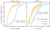 |
Fig. B.6. Cumulative distributions of ΔM30 and trise. The shaded regions represent the ±3σ confidence intervals estimated via Monte Carlo simulations. Five hundred realisations were generated for each distribution by perturbing the original measurements according to their associated uncertainties, assuming a Gaussian distribution. We computed the cumulative distribution function for each realisation and extracted the median, 0.3th percentile (lower bound), and 99.7th percentile (upper bound) to define the central trend and its corresponding error envelope. |
We identified SNe IIb outside this confidence region as potentially peculiar or misclassified objects. Eight such events were found: four (2017hyh, 2021udc, 2022psx, and 2024ljc) lie above the confidence region, exhibiting fast post-peak decline and short rise times; and four (2019hte, 2021iiu, 2022fzf, and 2022W) fall below the region, with fast rise times and slow post-peak decline.
The diagram shows that the first group of four SNe lies far from the SNe II region. As shown in Figure B.8, they all exhibit Hα in their spectra, ruling out a Type Ib classification. Therefore, we retained them in our sample. In contrast, the second group falls within the region populated by SNe II. Consequently, we categorise them as potential SNe II misclassified as IIb and remove them from our refined subsample of 59 SNe IIb for the robustness analysis presented in Section 4.5.
 |
Fig. B.7. Same as Figure B.5, but zoomed in after removing the objects excluded by the σ-clipping. A linear fit and its ±3σ confidence region are shown as a solid and dashed blue line, respectively. Using this correlation, we identify objects above and below the confidence region, marked with diamonds and hexagons. The black ellipse encloses those above the confidence region that show Hα features in their spectra (see Figure B.8). |
 |
Fig. B.8. Optical spectra of the four objects above the confidence region in Figure B.7. All four objects exhibit clear Hα features, confirming that they are indeed SNe IIb rather than SNe Ib. |
B.2.1. Peculiar SN 2022ytx
The spectrum of SN 2022ytx at −7.8 days relative to peak brightness matches that of SN IIb 2003bg at −7.4 days based on our method. This agrees with the report by Srivastav et al. (2022), which classified SN 2022ytx as a peculiar SNe IIb characterised by a long rise time (37.7 days) and a fast post-peak decline (ΔM15 = 2.23 mag). The classification report also highlights precursor emission detected in pre-explosion Pan-STARRS images approximately 60 days before discovery, although ATLAS data do not show this feature. We present our spectroscopic classification and light curve in Figures B.9 and B.10. The physical reason for explaining the peculiar light curve properties is unclear.
 |
Fig. B.10. Same as Figure B.2, but for SN 2022ytx. |
B.2.2. Misclassified SNe IIb as SNe II?
Within the original sample of 94 SNe II, we identify SN 2024pof as exhibiting an EE in its light curve (see Figure B.12), consistent with the EE observed in SNe IIb presented in this work. We classify this object as a SN II based on our spectral reclassification method. Figures B.11 and B.12 display its best spectral match and light curve, respectively. There are two possible interpretations for this object. The first is that it is indeed an SN II; however, to date, no SNe II have been reported to show such a pronounced EE. The second, and more likely scenario, is that SN 2024pof is a SN IIb whose only available spectrum, obtained at 9.42 days post-explosion, is too early and thus consistent with the spectral features of SNe II. Later-time spectra (e.g. at ∼20–25 days) would be necessary to confirm its classification as a SN IIb. As we noted, this issue directly impacts our results, implying that both the number of SNe IIb and the fraction exhibiting EE reported in this work should be considered lower limits.
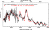 |
Fig. B.11. Same as Figure B.1, but for SN 2024pof. |
 |
Fig. B.12. Same as Figure B.2, but for SN 2024pof. |
Appendix C: Explosion epoch estimation
In this appendix, we detail the methodology used to determine the explosion epoch texp, including the estimation of the last non-detection and discovery epochs.
-
Pre-SN flux determination:
-
The pre-SN flux fpre − SN is defined as the median flux of all photometric points obtained before
 days.
days. -
The median
 and standard deviation σfpre − SN are computed using the median absolute deviation (MAD), which is robust against outliers:
-
Figure 1 (c) illustrates an example of the pre-SN flux determination.
-
-
Discovery epoch estimation:
-
The discovery time td is defined as the first photometric point satisfying:

where δfi is the flux uncertainty.
-
The following two consecutive epochs must also satisfy the above condition to confirm detection.
-
-
Last non-detection epoch estimation:
-
The last non-detection epoch tlnd is the latest photometric point before td that satisfies:

-
The choice of 1.5σ ensures that flux variations remain consistent with the pre-SN flux within reasonable statistical limits.
-
-
Explosion epoch and uncertainty calculation:
-
The explosion epoch is estimated as the midpoint between the last non-detection and discovery:
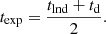
-
The uncertainty in the explosion epoch is given by:
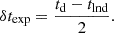
-
This methodology follows Taddia et al. (2015). Figure 1 (d) illustrates an example of the determination of tlnd and td in a real dataset.
-
Appendix D: Posterior distributions from the MCMC fit: SN 2022jpx
Figure D.1 shows the posterior distributions of the six SPM parameters obtained from the MCMC analysis of SN 2022jpx. These results provide the basis for estimating best-fit values and uncertainties.
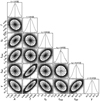 |
Fig. D.1. Posterior distributions of the six SPM parameters (A, f, t0, trise, tfall, γ) for SN 2022jpx. The distributions are based on MCMC sampling, with the median (50th percentile) indicated by vertical dashed lines, and shaded regions representing the 16th and 84th percentiles. The best-fit values and their associated errors are reported at the top of each panel. |
Appendix E: Light curve fitting and performance of the SPM
All SNe IIb light curves in our sample - with and without an EE detection - are displayed in Figures E.1 and E.2.
To evaluate the performance of the SPM, we analysed the residuals and the χdof2. To ensure consistent comparisons for all objects, we calculated residuals relative to the average flux between the explosion and 40 days later, removing biases associated with the brightness of specific SNe. Thus, we analysed the residuals by computing the mean, median, and standard deviation within a moving window of five days. Figure E.3 shows the relative residuals and their statistics. Generally, the relative errors are below 7.2% across most phases, except between days 10 and 15, where the relative error increases to 13%. This higher error is attributed to the rapid flux evolution during the rise time and the limited data points available in this phase, with an average of seven observations.
The χ2, which accounts for both residuals and the associated flux uncertainties, tends to be overestimated for brighter objects (fpeak > 1000 μJy). The reason is that brighter objects exhibit minor relative uncertainties than fainter ones, consistent with the Poisson nature of flux distributions, where the flux uncertainty scales as  , leading to higher χ2 values for brighter objects.
For the 63 SNe with a peak flux below 1000μJy, the mean, median, and standard deviation of the χdof2 are 3.5, 2.6, 3.1 respectively. In contrast, for the complete sample of 74 SNe, these values increase to a mean of 10.7, a median of 3, and a standard deviation of 35. The increase in χdof2 when including brighter objects highlights the effect above. This trend is further illustrated in Figure E.4, where a fainter object with larger mean residuals but higher relative errors exhibits a lower χdof2 compared to a brighter object with smaller mean residuals but lower relative errors.
Analysing the implications of these results for EE detection and light curve characterisation, we define EE detection in our methodology based on residual analysis, showing a maximum error of 13%, an acceptable uncertainty level. Additionally, during the post-peak phases, we measure all the parameters we use to characterise the light curves. The relative residuals are below 6% (see Figure E.3), ensuring robust analysis for subsequent studies.
Appendix F: Summary of distribution and correlation statistics
This appendix presents the full statistical analysis of light curve parameters for EE and non-EE SNe IIb discussed in Sections 4.2.1 and 4.2.2. Table F.1 summarises the Pearson correlation coefficients and p-values for the relationships between these parameters within the EE and non-EE samples, also evaluated across the same grid of δtexp and ρpeak thresholds. Table F.2 provides the results of the KS and AD tests applied to the distributions of trise, ΔM15, and  across a grid of explosion epoch error thresholds (δtexp ∈ [1, 2, …, 6]days) and observational point density thresholds (ρpeak ∈ [0.0.0.1,⋯,0.4] days−1).
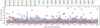 |
Fig. F.1. Relative residuals calculated concerning the average flux between the explosion and 40 days for the 74 SNe in the ATLAS sample. The pink and sation solid lines represent the mean and median estimates computed within a moving 5-day window, respectively, while the dashed lines represent the standard deviations. |
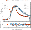 |
Fig. F.2. An illustrative example of χ2 overestimation for bright objects. The upper panel displays the light curves and SPM fits for SN 2024iss (red dots) and SN 2024jfg (blue dots), while the bottom panel shows their residuals. Within the upper panel, we report the number of observations, peak flux, and χdof2. The dashed lines in the bottom panel represent the values for three residual standard deviations. This example demonstrates how brighter objects with smaller residuals and lower relative errors can lead to an overestimation of χ2. |
Correlation coefficients between light curve parameters.
KS and AD test results for EE and non-EE SNe IIb.
All Tables
Number of SNe and spectra per SN type in the SNID and GELATO template libraries.
All Figures
|
Fig. 1. Data cleaning and explosion epoch estimation example for SN 2021zby. The panels, labelled as a, b, c, and d from top to bottom, present different stages of the analysis (we detail a and b in Section 2 and c and d in Section 3). Red and grey dots represent photometry in the o and c bands, respectively. Panel (a) shows the raw ATLAS forced photometry. Panel (b) presents the photometry after applying the ATClean methodology detailed in Section 2. Panel (c) shows the pre-SN photometry, where the red region highlights the relevant data, and the sky blue and brown dashed lines represent the 3 and 1.5 σpre − SN values, respectively. In Panel (d), green and black star symbols represent the last non-detection and discovery, which we use to estimate the explosion time. |
| In the text | |
|
Fig. 2. Distributions of fpeak, δtexp, ρpeak, and z for the SNe sample. Red and grey vertical dashed lines indicate the median and mean, respectively. |
| In the text | |
|
Fig. 3. Example of the SPM fit and refitting process for SN 2022jpx. The left panel shows the initial SPM fit, with outliers identified and enclosed by open blue squares in the top plot. The bottom plot displays the residuals associated with the SPM fit (rSPM), with dashed lines indicating the ±3σr thresholds used for outlier identification. From the left panel to the right, we illustrate the iterative SPM fitting process, where outliers are removed in each iteration until no outliers are detected. In this case, no outliers remain after the fifth iteration. The χd.o.f.2 value is reported in each panel for every iteration. |
| In the text | |
|
Fig. 4. Supernovae parametric model fits and residuals for 8 representative SNe IIb. The red points show the o-band photometry from ATLAS for each of the SNe in our sample. The black continuous line represents each SPM fit. Inside each panel, we indicate the name of the corresponding SN. Bottom Panels display the residuals of the SPM fit for each SN. The dashed lines mark the ±3σr thresholds, which we use to identify outliers. We excluded these outliers from the SPM refitting process. Cyan squares highlight the outliers, which we define as evidence for EE. |
| In the text | |
|
Fig. 5. Normalised light curves of the 20 EE SNe. The flux is normalised by the main peak flux in the o-band, illustrating the variability and timing of the EE among the sample. |
| In the text | |
|
Fig. 6. Supernovae counts and EE percentages under specific criteria. The number of SNe IIb satisfying specific criteria for observational point density (ρpeak > ρTH, left panel) and explosion epoch error (δtexp < δtTH, right panel) are shown as unfilled bars. Blue-filled bars represent the subset EE SNe. The dashed pink line indicates the percentage of EE SNe for each criterion, with numerical percentages displayed above the bars. |
| In the text | |
|
Fig. 7. Histograms and cumulative distributions of ΔM15, |
| In the text | |
|
Fig. 8. Correlation between ΔM15, trise, and |
| In the text | |
|
Fig. 9. Evolution of the g − r colour for EE and non-EE SNe up to 30 days post-explosion. Individual measurements for non-EE SNe are shown as grey points, while pastel-coloured markers represent EE SNe. The solid lines correspond to the centred moving averages, pink for EE and sation for non-EE SNe. Dashed lines indicate the standard deviation (σ) per time bin, and the shaded regions denote the mean ± σ. The vertical black line marks the median upper limit of the EE duration (8 days). |
| In the text | |
|
Fig. 10. Normalized light curves of nine SNe with SC emission compiled from the literature, presented in different photometric bands. Analogous to Figure 5, the light curves are normalized by the flux of the second peak, illustrating the diversity of SC properties. Solid lines represent the ALR interpolation of the first and second peaks, while the dashed line represents the transition between the two peaks. |
| In the text | |
|
Fig. 11. Correlation analysis between parameters measured during the shock SC phase and those associated with the main peak of the light curve for the literature sample. Significant correlations are highlighted, including relationships within the SC phase, such as between the transitional absolute magnitude (Mtrans) and the SC rise time (trise), and between the SC peak absolute magnitude (Mpeak, SC) and Mtrans. Correlations within the main peak include Mpeak and trise. Additionally, correlations between the SC phase and the main peak are shown, including ttrans with trise, Mpeak, SC with trise, and Mpeak, SC with Mpeak. These relationships provide evidence linking the SC phase to the main peak properties, highlighting the continuity of physical processes across both phases. Non-significant correlations are also shown for completeness. |
| In the text | |
|
Fig. 12. B − V colour evolution for SNe with (seven) and without (five) SC up to 30 days post-explosion. Individual data points for SNe without SC are sation, while pastel-coloured markers represent those with SC. Solid lines show the centred moving averages, with pink representing SNe with SC and sation for those without SC. Dashed lines indicate the standard deviation (σ) around the mean for each time interval, and the filled regions represent the mean ± σ. The vertical black line marks the average upper limit for the SC duration. Analogous to Figure 9, this figure emphasizes the differences in colour evolution between the two groups, particularly in the early phases. |
| In the text | |
|
Fig. 13. Zwicky Transient Facility verification of potential false positives with ZTF photometry. The top panels show the ATLAS o-band photometry, with potential SC points enclosed by blue open squares. The middle panels illustrate the residuals produced by the SPM model. The bottom panels display the ZTF g- and r-band photometry, with points consistent with an EE identified by visual inspection and enclosed in purple open circles. |
| In the text | |
|
Fig. 14. Same as Figure 6 using our defined cleaned sample after rejecting potential false positive EE SNe. |
| In the text | |
|
Fig. 15. Same as Figure 7, but after removing potential false positives among EE SNe (Section 4.5.1) and possibly misclassified objects (Section 2), reducing the sample from 66 to 59 SNe. |
| In the text | |
|
Fig. 16. Same as Figure 8, but after removing potential false positives among EE SNe (Section 4.5.1) and possibly misclassified objects (Section 2), reducing the sample from 66 to 59 SNe. |
| In the text | |
|
Fig. B.1. Supernova Identification best template match of SN 2022yep (black line) with SN 2006bp (red line). The phase of each spectrum relative to the light curve peak is indicated in the figure. |
| In the text | |
|
Fig. B.2. ATLAS o-band light curve of SN 2022yep. The continuous black line shows the fit using the SPM. Red and blue dots correspond to the photometry in the o and c ATLAS bands, respectively. The bottom panel shows the residuals of the SPM fit, with dashed lines indicating the ±3σr range. |
| In the text | |
|
Fig. B.3. Supernovae parametric model fits and residuals for 27 SNe II. Orange circles show the ATLAS o-band photometry for each SN. Solid black lines represent the corresponding SPM fits. The name of each SN is indicated in the upper right corner of each light curve panel. Bottom panels display the residuals between the photometry and the SPM fits. The shaded green area marks the ±3σr region, and dashed orange lines indicate the ±3σr thresholds. |
| In the text | |
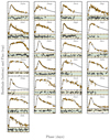 |
Fig. B.4. Same as Figure B.3, but for 25 additional SNe II. |
| In the text | |
|
Fig. B.5. SNe IIb (blue dots) and SNe II (orange dots) in the trise–ΔM30 parameter space. Objects rejected through the spectroscopic reclassification method described in Section B.1 are marked with filled X symbols. Additionally, objects excluded after the σ-clipping procedure are shown with unfilled X markers. The number of SNe II and IIb in the sample is indicated, along with the correlation test result for SNe IIb. |
| In the text | |
|
Fig. B.6. Cumulative distributions of ΔM30 and trise. The shaded regions represent the ±3σ confidence intervals estimated via Monte Carlo simulations. Five hundred realisations were generated for each distribution by perturbing the original measurements according to their associated uncertainties, assuming a Gaussian distribution. We computed the cumulative distribution function for each realisation and extracted the median, 0.3th percentile (lower bound), and 99.7th percentile (upper bound) to define the central trend and its corresponding error envelope. |
| In the text | |
|
Fig. B.7. Same as Figure B.5, but zoomed in after removing the objects excluded by the σ-clipping. A linear fit and its ±3σ confidence region are shown as a solid and dashed blue line, respectively. Using this correlation, we identify objects above and below the confidence region, marked with diamonds and hexagons. The black ellipse encloses those above the confidence region that show Hα features in their spectra (see Figure B.8). |
| In the text | |
|
Fig. B.8. Optical spectra of the four objects above the confidence region in Figure B.7. All four objects exhibit clear Hα features, confirming that they are indeed SNe IIb rather than SNe Ib. |
| In the text | |
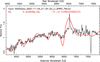 |
Fig. B.9. Same as Figure B.1, but for SN 2022ytx |
| In the text | |
|
Fig. B.10. Same as Figure B.2, but for SN 2022ytx. |
| In the text | |
|
Fig. B.11. Same as Figure B.1, but for SN 2024pof. |
| In the text | |
|
Fig. B.12. Same as Figure B.2, but for SN 2024pof. |
| In the text | |
|
Fig. D.1. Posterior distributions of the six SPM parameters (A, f, t0, trise, tfall, γ) for SN 2022jpx. The distributions are based on MCMC sampling, with the median (50th percentile) indicated by vertical dashed lines, and shaded regions representing the 16th and 84th percentiles. The best-fit values and their associated errors are reported at the top of each panel. |
| In the text | |
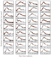 |
Fig. E.1. Same as Figure 4, for 36 objects. |
| In the text | |
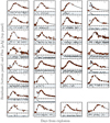 |
Fig. E.2. Same as Figure E.1, for the remaining 30 objects. |
| In the text | |
|
Fig. F.1. Relative residuals calculated concerning the average flux between the explosion and 40 days for the 74 SNe in the ATLAS sample. The pink and sation solid lines represent the mean and median estimates computed within a moving 5-day window, respectively, while the dashed lines represent the standard deviations. |
| In the text | |
|
Fig. F.2. An illustrative example of χ2 overestimation for bright objects. The upper panel displays the light curves and SPM fits for SN 2024iss (red dots) and SN 2024jfg (blue dots), while the bottom panel shows their residuals. Within the upper panel, we report the number of observations, peak flux, and χdof2. The dashed lines in the bottom panel represent the values for three residual standard deviations. This example demonstrates how brighter objects with smaller residuals and lower relative errors can lead to an overestimation of χ2. |
| In the text | |
Current usage metrics show cumulative count of Article Views (full-text article views including HTML views, PDF and ePub downloads, according to the available data) and Abstracts Views on Vision4Press platform.
Data correspond to usage on the plateform after 2015. The current usage metrics is available 48-96 hours after online publication and is updated daily on week days.
Initial download of the metrics may take a while.