A comprehensive catalogue of high-mass X-ray binaries in the Large Magellanic Cloud detected during the first eROSITA all-sky survey

D. Kaltenbrunner; C. Maitra; F. Haberl; J. Bodensteiner; D. Bogensberger; D. A. H. Buckley; M. R. L. Cioni; J. Greiner; I. Monageng; A. Udalski; G. Vasilopoulos; R. Willer

doi:10.1051/0004-6361/202555693

Home

All issues

Volume 707 (March 2026)

A&A, 707 (2026) A225

Full HTML

Open Access

Issue		A&A Volume 707, March 2026


Article Number		A225
Number of page(s)		38
Section		Catalogs and data
DOI		https://doi.org/10.1051/0004-6361/202555693
Published online		17 March 2026

A&A, 707, A225 (2026)

A comprehensive catalogue of high-mass X-ray binaries in the Large Magellanic Cloud detected during the first eROSITA all-sky survey

D. Kaltenbrunner¹^★, C. Maitra¹^,2^★, F. Haberl¹, J. Bodensteiner³^,4, D. Bogensberger⁵^,6, D. A. H. Buckley⁷^,8, M. R. L. Cioni⁹, J. Greiner¹, I. Monageng⁷^,8, A. Udalski¹⁰, G. Vasilopoulos¹¹^,12 and R. Willer¹

¹ Max-Planck-Institut für extraterrestrische Physik, Gießenbachstraße 1, 85748 Garching, Germany
² Inter-University Centre for Astronomy and Astrophysics (IUCAA), Ganeshkhind, Pune 411007, India
³ ESO − European Southern Observatory, Karl-Schwarzschild-Straße 2, 85748 Garching bei München, Germany
⁴ Anton Pannekoek Institute for Astronomy, University of Amsterdam, Science Park 904, 1098 XH Amsterdam, The Netherlands
⁵ Department of Astronomy, The University of Michigan, 1085 South University Avenue, Ann Arbor, Michigan, 48103, USA
⁶ Université Paris-Saclay, Université Paris Cité, CEA, CNRS, AIM, 91191 Gif-sur-Yvette, France
⁷ Southern African Astronomical Observatory, PO Box 9, Observatory Rd, Observatory 7935, South Africa
⁸ Department of Astronomy, University of Cape Town, Private Bag X3, Rondebosch 7701, South Africa
⁹ Leibniz Institut für Astrophysik Potsdam, An der Sternwarte 16, 14482 Potsdam, Germany
¹⁰ Astronomical Observatory, University of Warsaw, Warszawa, Poland
¹¹ Department of Physics, National and Kapodistrian University of Athens, University Campus Zografos, GR 15784, Athens, Greece
¹² Institute of Accelerating Systems & Applications, University Campus Zografos, Athens, Greece

^★ Corresponding author: This email address is being protected from spambots. You need JavaScript enabled to view it. ; This email address is being protected from spambots. You need JavaScript enabled to view it.

Received: 28 May 2025
Accepted: 2 January 2026

Abstract

Context. The Magellanic Clouds, the closest star-forming galaxies to the Milky Way, offer an excellent environment to study high-mass X-ray binaries (HMXBs). While the Small Magellanic Cloud (SMC) has been thoroughly investigated with over 120 systems identified, the Large Magellanic Cloud (LMC) has lacked a complete survey due to its large angular size. Most prior studies targeted central or high-star-formation regions. The SRG/eROSITA all-sky surveys now enable a comprehensive coverage of the LMC, particularly due to its close vicinity to the south ecliptic pole.

Aims. This work aims to improve our understanding of the HMXB population in the LMC by building a flux-limited catalogue. This allows us to compare sample properties with those of HMXB populations in other nearby galaxies.

Methods. Using detections during the first eROSITA all-sky survey (eRASS1), we cross-matched X-ray positions with optical and infrared catalogues to identify candidate HMXBs. We assigned flags based on multi-wavelength follow-up observations and archival data, using properties of known LMC HMXBs. These flags defined confidence classes for our candidates.

Results. We detect sources down to X-ray luminosities of a few 10³⁴ erg s⁻¹, resulting in a catalogue of 53 objects, including 28 confirmed HMXBs and 21 new eROSITA detections. Compared to the SMC, the LMC hosts fewer HMXBs and more systems with supergiant companions. We identify several likely supergiant systems, including a candidate supergiant fast X-ray transient with phase-dependent flares. We also find three Be stars with likely white dwarf companions. Two of the candidate Be/WD binaries show steady luminosities across four eROSITA scans, unlike the post-nova states seen in the majority of previous Be/WD reports.

Conclusions. Our catalogue is the first to cover the entire LMC since the ROSAT era, providing a basis for statistical population studies. Using the HMXB population, we estimate the LMC star-formation rate to be (0.22_−0.07^+0.06) M_⊙yr⁻¹, which is in agreement with results using other tracers.

Key words: stars: emission-line, Be / stars: neutron / supergiants / white dwarfs / galaxies: individual: LMC / X-rays: binaries

© The Authors 2026

Open Access article, published by EDP Sciences, under the terms of the Creative Commons Attribution License (https://creativecommons.org/licenses/by/4.0), which permits unrestricted use, distribution, and reproduction in any medium, provided the original work is properly cited.

This article is published in open access under the Subscribe to Open model.

Open Access funding provided by Max Planck Society.

1 Introduction

High-mass X-ray binaries (HMXBs) are instrumental in studying the final stages of massive star evolution and their interactions with compact objects such as neutron stars (NSs) or black holes (BHs; Liu et al. 2006; Remillard & McClintock 2006). These systems consist of an early-type (O or B) massive (≳8 M_⊙) star and a compact companion, where the compact object accretes material from the stellar wind or via Roche lobe overflow, leading to diverse X-ray emission, ranging from persistent to highly transient behaviour, and can be among the brightest X-ray sources in the sky (Reig & Nespoli 2013).

The Large Magellanic Cloud (LMC) serves as an excellent environment for investigating HMXBs due to its proximity (∼50 kpc Pietrzyński et al. 2019) and low foreground absorption (Harris & Zaritsky 2009). Additionally, the LMC exhibits a high specific star formation rate (SFR) similar to that of the Small Magellanic Cloud (SMC) and significantly higher than that of the Milky Way (MW; Harris & Zaritsky 2004, 2009), as well as a metallicity approximately half of that of our galaxy, and approximately twice of that of the SMC (Rolleston et al. 2002; Luck et al. 1998).

Additionally, the LMC’s large angular extent, approximately 10 degrees by 10 degrees on the sky, has limited deep sensitive studies mainly to its central regions (Maggi et al. 2016) as compared to the SMC (Sturm et al. 2013). While ROSAT covered the entire LMC, the observations were constrained by a relatively low sensitivity and positional precision, and a narrow soft energy range (0.1–2.4 keV).

The known HMXB population in the LMC is dominated by Be/X-ray binaries (BeXRBs), which are the most common sub-class of HMXBs in metal-poor, actively star-forming environments. These systems typically consist of a NS orbiting a Be-type donor star, with mass transfer occurring episodically through interactions with the circumstellar disc. Their X-ray spectra are characterised by a hard power-law continuum with power-law indices of ∼1. Typically, BeXRBs show high variability, seen in Type I outbursts (modulated by the orbital period) and occasional giant Type II outbursts, where the X-ray luminosity can increase by several orders of magnitude (e.g. Vasilopoulos et al. 2020; Yang et al. 2025).

The observed HMXB population in the LMC provides valuable insights into how metallicity and star formation history (SFH) influence the formation and evolution of compact object binaries. Compared to the SMC, the fraction of supergiant X-ray binaries (SgXRBs) is higher in the LMC. This can be mainly attributed to differences in the SFH. In the SMC, the HMXB population is caused predominantly by high star formation activity 25−40 Myr ago (Antoniou et al. 2010). To date, the SMC is known to host ∼130 BeXRBs and only one SgXRB (Haberl & Sturm 2016). The HMXB population in the LMC is associated with a star formation period at an earlier epoch and at a lower HMXB formation efficiency (Antoniou & Zezas 2016). Out of the 59 HMXBs known to date, 8 are SgXRBs, such as LMC X−1, LMC X−3, and LMC X−4, and more recent discoveries such as supergiant fast X-ray transient (SFXT) systems (Vasilopoulos et al. 2018). The higher number of HMXBs in the SMC despite its lower stellar mass compared to the LMC (SMC: ∼ 3.2 × 10⁸M_⊙, LMC: ∼ 1.3 × 10⁹M_⊙; Skibba et al. 2012) can be attributed to the interplay between recent SFH and metallicity (Linden et al. 2010).

The eROSITA instrument aboard the Spektrum Roentgen Gamma (SRG) spacecraft (Sunyaev et al. 2021; Predehl et al. 2021) has drastically improved the detection and cataloguing of X-ray sources, particularly in the LMC. The first eROSITA all-sky survey (eRASS1) provides enhanced sensitivity and positional accuracy, which is particularly beneficial in the LMC due to its proximity to the south ecliptic pole (SEP), where all eROSITA scans overlap. This overlap results in some parts of the LMC, especially those near the SEP, being observed for in total over 50 ks over the first four eROSITA all-sky surveys (eRASS:4), enabling detailed studies of this region (Merloni et al. 2024). Compared to ROSAT, eROSITA is about 25 times more sensitive in the soft band (0.2–2.3 keV), while in the hard band (2.3–8.0 keV) it provides the first imaging survey of the entire LMC (Predehl et al. 2021).

In this paper, we present a new catalogue of HMXBs in the LMC based on objects detected during eRASS1. To validate and further characterise these sources, we use properties of known LMC HMXBs. We use photometric data from the Mag-ellanic Clouds Photometric Survey (MCPS; Zaritsky et al. 2002, 2004) and the VISTA Magellanic Cloud Survey (Cioni et al. 2011). We assess LMC membership using proper motion measurements from Gaia eDR3 (Gaia Collaboration 2021). We study optical variability with light curves from the Optical Gravitational Lensing Experiment (OGLE; Udalski et al. 2015). We also incorporate optical follow-up spectroscopy with the FLOYDS spectrograph mounted on the 2 m Las Cumbres Observatory (LCO; Brown et al. 2013) telescope at Siding Spring Observatory in Australia, the Robert Stobie Spectrograph (RSS), and the High Resolution Spectrograph (HRS), both on the 9.2 m Southern African Large Telescope (SALT). Finally, we include X-ray observations from XMM-Newton. We also leverage archival data from the VizieR¹ database, the ESO Archive Science Portal², and the HILIGT upper limit server³ (Saxton et al. 2022).

For new candidate HMXBs, we apply a system of flags to assess their credibility, taking into account multi-wavelength information and additional follow-up observations. Moreover, X-ray spectra and light curves for these sources are derived from data collected across all four eROSITA all-sky surveys (eRASS1−eRASS4). This approach allows us to make detailed inferences about all the candidates by assigning confidence classes. Following this, we derive a flux-limited catalogue of HMXBs in the entire LMC.

The paper is organised as follows. Section 2 focuses on the instruments used for the detailed analysis of sources in our catalogue. In Sect. 3 we explain the criteria we used for objects to enter our catalogue. Section 4 then focuses on how we analysed the multi-wavelength data to obtain the parameters and characteristics of interest. In Sect. 5 we discuss the properties of the whole sample, and explain the scheme for the classification of all sources in our catalogue into six confidence classes of (candidate) HMXBs. Additionally, this section explains the flags we used for assigning confidence classes. In Sect. 6 we discuss the X-ray luminosity function, a fundamental relation that links HMXBs with the SFR of a galaxy. In Sect. 7 we discuss our results for individual objects, examine optical variability and the classification of optical counterparts, and compare our overall findings with those from previous studies in the SMC. Finally, in Sect. 8 we summarise our findings. Following Pietrzyński et al. (2019), we assume a distance of d = 49.49 kpc to the LMC in this paper.

2 Observations

2.1 eROSITA

The main instrument we used for our analysis is eROSITA (Predehl et al. 2021), the soft X-ray instrument on board the SRG mission, which was launched in 2019 and surveyed the whole X-ray sky in great circles passing through the ecliptic poles between December 2019 and February 2022 in the energy range of 0.2– 8 keV. We investigated sources that were detected during the first eROSITA all-sky survey (eRASS1, Merloni et al. 2024) and analysed the combined data products of all eROSITA scans. Due to its close vicinity to the SEP, sources in the direction of the LMC were monitored for a significantly longer period than the rest of the sky, with average effective exposures (corrected for vignetting) that are higher by between one and two orders of magnitude. During eRASS1, effective exposures (0.2−4.5 keV) in the LMC range from 406 to 28 218 s, with a median value of 1064 s. The effective exposure at the ecliptic equator is ∼100 s (Merloni et al. 2024).

2.2 XMM-Newton

XMM-Newton (X-ray Multi-Mirror mission; Jansen et al. 2001) is an X-ray observatory launched by the European Space Agency in 1999. For our analysis, we utilised data from the three European Photon Imaging Cameras (EPIC), comprising two MOS-CCD cameras (Turner et al. 2001) and one pn-CCD camera (Strüder et al. 2001). We used data from XMM-Newton for more detailed X-ray analysis and to search for possible pulse periods of objects we found during our eROSITA analysis. XMM-Newton data additionally provides more precise astromet-rical positions (median uncertainty of 0.9^′′ for XMM-Newton positions of HMXBs in the LMC performing source detection using the standard XMM-Newton pipeline similar to Haberl et al. 2025) and a way to validate optical counterparts.

2.3 OGLE monitoring

We used photometric data from the regular monitoring of the LMC by the OGLE project (Udalski et al. 1992). Images were taken at the Las Campanas Observatory in the I and (less frequently) V bands with the 1.3 m Warsaw telescope starting in 1997 (OGLE-II). During phases OGLE-III (begin 2001) and OGLE-IV (begin 2010), improved CCDs with an increased field of view (FOV) were used. The data were calibrated to the standard I-band system in the manner described in Udalski et al. (2008, 2015). The OGLE data used in this work are summarised in Table D.1. Most of our objects were covered by OGLE-IV for about 14 years, while for those also observed during OGLE-III, light curves ≳23 years are available. The typical observing cadence for our sources (median time interval between observations) is two or three days, but can be longer in a few cases (e.g. sources 10 and 28 from Table D.1, with 4 and 7 days, respectively). On the other hand, some selected fields are observed up to eight times per night for selected observing seasons (e.g. sources 36 and 43).

2.4 LCO/FLOYDS spectroscopy

To characterise the optical counterpart of objects in our catalogue, we used spectroscopic data from the LCO/FLOYDS spectrograph that was commissioned at Faulkes Telescope South (FTS) at Siding Springs Observatory in 2012. Observations were planned to achieve a signal-to-noise ratio (S/N) of ≈100 with a resolving power of 326−384 in the 5600–6600 Å range and 482−588 in the 4100–5000 Å range. To reduce spectra,

PyRAF

tasks were used as part of the FLOYDS pipeline⁴ in the manner explained in Valenti et al. (2013). We analysed the Hα and Hβ lines that typically appear in emission in Be stars (Porter & Rivinius 2003; Balona 2000; Slettebak 1988). Table 1 gives details on each observation we used.

2.5 SALT/RSS and SALT/HRS spectroscopy

Additional optical spectroscopy was undertaken using the RSS and the HRS on SALT (first light in 2005) under the SALT transient follow-up programme. For the RSS, the PG0900 VPH grating was used, which covers the spectral region 3920–7000 Å at a resolving power of 632–1129. For the HRS, we used the low resolution mode with a resolving power of ∼16 000 in the spectral region 3700–8900 Å. The SALT pipeline was used to perform primary reductions comprising overscan corrections, bias subtraction, gain correction, and amplifier cross-talk corrections (Crawford et al. 2010). The remaining steps, which include wavelength calibration, background subtraction, and extracting the 1D spectrum, were executed using IRAF⁵. Table 1 lists information on all individual observations taken with SALT.

2.6 VLT FLAMES/GIRAFFE spectroscopy

We made use of archival optical spectra obtained with the Fibre Large Array Multi Element Spectrograph (FLAMES), which started its operations in 2001 at the 8.2 m Unit Telescope 2 (UT2) of the Very Large Telescope (VLT) at Cerro Paranal, Chile (Pasquini et al. 2002). The spectra we used were obtained with the GIRAFFE spectrograph, which has a resolving power of 17 000 in the spectral region 6299–6691 Å, and were processed using the standard data reduction pipeline (Evans et al. 2011).

2.7 Broad-band photometry

In order to get an additional assessment of whether the spectral energy distribution (SED) is consistent with that of an early-type star in the LMC, we compared all available photometric measurements with synthetic models. For the observations, we used the VizieR photometry tool and obtained all available photometric measurements within a 1^′′ circle around the source position. This approach is supported by the availability of data from survey missions such as 2MASS, Gaia, IRAC, and WISE for the majority of our sources. All flux values were converted to common units of erg cm⁻² s⁻¹ Å⁻¹.

3 Building the catalogue

In this section we explain the catalogues and steps required to create our initial set of HMXBs. In Sect. 5.6, these candidates are then rated more precisely by comparing parameters with those of all secure HMXBs in our catalogue and of possible contaminators such as active galactic nuclei (AGNs) or foreground stars.

3.1 Catalogues used

3.1.1 eRASS1 source catalogue

As a basis for our analysis, we used the first eROSITA All-Sky Survey (eRASS1; Merloni et al. 2024). Most HMXBs are spectrally hard sources, which in the LMC can be very useful because they stand out against the soft X-ray emission caused by the hot interstellar medium, which is especially dominant in the centre of the LMC. To utilise this, we used two different eRASS1 catalogues. The first is the publicly released one-band (1B) catalogue for which source detection in the most sensitive band of eROSITA between 0.2 and 2.3 keV was applied. As a complementary catalogue to reduce the impact of the hot ISM in the LMC centre and to increase the sensitivity for hard sources, we used a catalogue for which source detection was applied in three energy bands simultaneously (3B catalogue; the bands are 0.2−0.6 keV, 0.6−2.3 keV, and 2.3−5.0 keV). This catalogue was published by Merloni et al. (2024), but they used an additional cut of a minimum detection likelihood in the hardest band

DET_LIKE_3

≥12. This cut proved overly restrictive for our purposes, and we therefore did not apply it.

The positional uncertainties of the 1B catalogue are given in the

POS_ERR

column. This column corrects the uncertainties found during source detection (

RADEC_ERR

) by analysing distances found during matching the eRASS1 source catalogue with AGN catalogues as is described in Sect. 6.2 of Merloni et al. (2024). The correlation between

POS_ERR

and

RADEC_ERR

is given by

POS_ERR = \sqrt{A \cdot σ^{2} + σ_{0}^{2}},

$Mathematical equation: ${\rm{POS\_ERR}} = \sqrt {A \cdot {\sigma ^2} + \sigma _0^2} ,$$

where $σ = RADEC_ERR / \sqrt{2}$ $Mathematical equation: $\sigma = {\rm{RADEC\_ERR}}/\sqrt 2 $$ , A, and σ₀ are the multiplicative and the systematic correction terms, respectively. To test whether this correction also applies to the higher-exposure LMC region and if it can be applied to the 3B catalogue, we conducted a similar but simplified analysis for Gaia-detected AGNs in the LMC region. For both catalogues, we find both correction terms in agreement within uncertainties with those from Merloni et al. (2024), which are A = 1.3 and σ₀ = 0.9. Given our smaller sample compared to the one used by Merloni et al. (2024), we therefore used the

POS_ERR

as positional uncertainties of the 1B catalogue and applied the same correction for objects in the 3B catalogue.

Due to the close vicinity of the LMC to the SEP, the exposure varies highly from the east to the west end (see Fig. 1). This has its strongest influence on population analysis, such as completeness (see Sect. 5.6) and the extraction of a completeness-corrected luminosity function (see Sect. 6).

To reduce the contribution of spurious detections and chance coincidences, we applied three cuts to the eRASS1 catalogue. The first was to select only point-like sources by requiring log-likelihood of the extent probability

EXT_LIKE

=0. This cut applied to 7 and 6% of detections in the LMC listed in the 1B and 3B catalogues, respectively. By selecting only catalogue objects with positional uncertainties within the lower 95 percent of all objects within the LMC, we made sure not to include sources for which a secure identification of the optical and infrared (IR) counterparts could not be achieved. This resulted in a maximum

POS_ERR

of 6.92^′′ and 6.96^′′ for the 1B and 3B catalogues, respectively. Next, we applied

DET_LIKE_0

≥20, which we found to be most useful in restraining the number of spurious detections caused by the hot ISM. In the 1B catalogue,

DET_LIKE_0

refers to the detection log-likelihood in the 0.2−2.3 keV band; in the 3B catalogue, it refers to the combined detection likelihood in all three bands. For fainter sources, it is typically not possible to securely identify an object as a source, and even less so to constrain the spectral parameters well enough to distinguish an HMXB from contaminating objects. This cut applies to 64 and 66% of detections in the LMC listed in the 1B and 3B catalogues, respectively. Finally, the remaining spurious objects were identified and sorted out through visual screening using RGB images of eRASS1−4 and eRASS:4 covering the sources. This visual screening was conducted during the final step of matching the eRASS1 catalogues with optical and IR catalogues (see Sect. 3.2).

Table 1

Summary of spectroscopic observations done for objects in our catalogue.

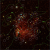Fig. 1

RGB (r: 0.2−1.0 keV, g: 1.0−2.0 keV, b: 2.0−4.5 keV) of LMC during eRASS 1. The green contours show the total exposure achieved with eRASS1. The exposure maximum lies at the SEP. Cyan markers represent known HMXBs. Red and yellow markers show candidates, representing previously known objects and those discovered with eROSITA, respectively. Labels refer to the sequence numbers in Table 5. The entire region visible in the image, except for the top corners, was investigated during our analysis. White contours indicate the LMC coverage by XMM-Newton. Remarkably, the central LMC has been thoroughly observed by XMM-Newton, while the outskirts remain under-sampled.

3.1.2 MCPS

The Magellanic Clouds Photometric Survey is a four-band (U, B, V, and I) survey of the LMC and SMC with a typical astrometric uncertainty of less than 1^′′ (Zaritsky et al. 2002, 2004). For the LMC, the central 8 × 8 deg² were covered down to a typical limiting magnitude of V=21 mag. Sturm et al. (2013) have shown that the early-type optical companions in HMXBs can be found using a colour and magnitude selection of secure HMXBs. We used the criteria 12.0 mag<V<16.4 mag and −0.6 mag<B−V<0.7 mag, which we got from the distribution of known HMXBs (see Fig. 2). We slightly relaxed the selection criteria by requiring that the selection criteria have to be fulfilled within the uncertainties listed in the MCPS catalogue.

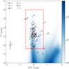Fig. 2

Selection of MCPS counterparts (red rectangle) compared to the distribution of MCPS entries matched with the Gaia proper motion selection for the LMC (colour mesh; found by matching the MCPS catalogue with Gaia proper motion selection). The colour scale gives the number of sources in each colour-magnitude bin. The bin sizes are 0.01 mag and 0.02 mag for B−V and V, respectively. Data points show the MCPS counterparts of all objects in our catalogue grouped by their confidence classes. Note that #11 was not used for defining the selection criterion, because the absence of I-band and U-band measurements in the MCPS catalogue indicates a possible measurement error. We include objects #48 and #49 in our selection because our criterion allows objects to be considered as long as they fall within the selection region when accounting for uncertainties. Objects #38 and #47 are considered candidates because their VMC counterparts meet the VMC selection criteria described in Sect. 3.1.3.

3.1.3 VMC

The VISTA (VISual and infrared Telescope for Astronomy) near-IR YJK_S survey of the Magellanic Cloud system (VMC; Cioni et al. 2011) has an astrometric uncertainty of less than 1^′′ for 98.4% of the sources. By observing stars across multiple wavelengths, VMC aims to analyse stellar populations, map their three-dimensional structure, identify variable stars, and investigate SFH. The survey was designed to achieve S/N=10 at Y=21.1 mag, J=21.3 mag, and Ks=20.7 mag, respectively. For our study we used DR6 of the VMC catalogue (Cioni & et al. 2023). Similar to the MCPS selection, we used the distribution of known HMXBs to define a selection criterion for the candidates. We required 12.8 mag<Y<16.6 mag, −0.126 mag<Y−J<0.251 mag, and −0.142 mag<J−Ks<0.485 mag. As is seen in Fig. 3, this selection is well separated from the colour-colour region that quasars typically reside in (Cioni et al. 2013).

3.1.4 Gaia EDR3

To verify the LMC membership of the MCPS and VMC counterparts, we used the spatial and proper motion selection criterion of the LMC from Gaia EDR3 presented in Sect. 2 in Gaia Collaboration (2021). We also used the more precise Gaia positions for matching between different optical and IR catalogues.

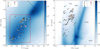Fig. 3

Left: distribution of VMC counterparts of all sources in our catalogue grouped by confidence class (see Table 7) in the VMC colour-colour plane compared to the typical location of QSOs marked by the dotted line (see Cioni et al. 2013, Eq. (1)–(3)) and the distribution of LMC stars (colour mesh; found by matching VMC with Gaia proper motion selection). The colour scale gives the number of sources in each colour-colour bin. The bin sizes are 0.01 mag for both axes. Right: sources in our catalogue in the colour-magnitude plane compared to different stellar evolution stages and features caused by foreground and background objects (see Sun et al. 2017, their Fig. 2 and Sect. 3.1; MS: main-sequence, RGB: red giant branch, RC: red clump, RSG: red supergiants, FGS: foreground Galactic stars, BGG: background galaxies) and LMC stars (colour mesh). The colour scale gives the number of sources in each colour-magnitude bin. The bin sizes are 0.01 and 0.02 mag for Y−J and Ks, respectively.

3.1.5 Known HMXBs

We utilised existing literature (Haberl & Pietsch 1999a; Sasaki et al. 2000; Antoniou & Zezas 2016; Vasilopoulos et al. 2013a; Haberl et al. 2022, 2023; Maitra et al. 2019a, 2021a,b, 2023b; van Jaarsveld et al. 2018) to identify known HMXBs and their characteristics. By analysing these sources, we established parameter ranges for selecting new HMXB candidates.

3.1.6 Screening catalogues

To obtain a reliable HMXB catalogue, it is essential to screen other kinds of securely identified X-ray point sources. The majority of sources possibly contaminating our catalogue are AGNs behind the LMC that match an LMC early-type star by chance coincidence. The accretion of matter onto supermassive BHs can produce similar X-ray spectra as HMXBs, but they can more easily be discriminated using data from other wavelengths, especially using mid-IR and far-IR data. Other possible contaminators of our catalogue are galaxies behind the LMC that appear as point sources for eROSITA, cataclysmic variable stars, or foreground MW stars. For screening, we used the catalogues listed in Table 2. We used only subsets defined by the rules listed in the table to avoid falsely excluding HMXBs listed in those catalogues. Entries of the catalogues that fulfil the criteria in the ‘Flags’ column are treated as candidates. Each source in our catalogue that matches one of those candidates is flagged and considered an HMXB candidate of lower reliability.

3.2 Catalogue matching

A schematic of the matching process to arrive at the final list of HMXB candidates is shown in Fig. 4. The fundamental catalogues of HMXB candidates were derived from matching the eRASS1 1B catalogue with optical or IR counterparts from the MCPS and VMC catalogues, respectively. Complementary to this, we utilised the eRASS1 3B catalogue to search for very faint, hard sources that would be missed when using the 1B catalogue alone. In total, this results in four lists that we combined into a final catalogue of HMXB candidates in the last step. The detailed steps are the following:

Known HMXB (candidates) in eRASS1: we matched the full eROSITA catalogue with the X-ray positions of our list of previously known HMXB (candidates) with a maximum separation of 30^′′ to minimise the risk of chance-coincidences. Additionally, we implied a maximum separation of less than or equal to 3σ. For a Rayleigh distribution, this is equivalent to $S e p a r a t i o n \leq 3.439 \cdot \sqrt{POS_{ERR}^{2} + σ_{X - r a y}^{2}}$ $Mathematical equation: $Separation \le 3.439 \cdot \sqrt {{\rm{POS}}\_{\rm{ER}}{{\rm{R}}^{\rm{2}}}{\rm{ + }}\sigma _{X - ray}^2}$$ , where σ_X−ray is the X-ray positional error of previous observations. If eROSITA improved the positional uncertainty of a candidate and the new position no longer matched that of an early-type star from our MCPS and VMC selections, we rejected the candidate as a possible HMXB.
eRASS1 LMC catalogue: contains all eRASS1 sources with distances <10 degrees to the centre of the LMC at RA=05h 23 m 34.00s and Dec=−69d 45 m 22.0s (1B: 50148 objects, 3B: 50914 objects).
Cleaned eRASS1 LMC catalogue: from the eRASS1 LMC catalogue, we selected only the objects with
```
DET_LIKE_0
```
≥ 20 and
```
EXT_LIKE
```
=0 (1B: 15770 objects, 3B: 15229 objects).
Screened and cleaned eRASS1 LMC catalogue: to clean the eRASS1 catalogue from known foreground and background X-ray sources, we removed from the eRASS1 catalogue matches with the screening catalogues found in Table 2 within a search radius of 30" and a maximum separation of less than or equal to $3 σ = 3.439 \cdot \sqrt{POS_{ERR}^{2} + σ_{s c r e e n}^{2}}$ $Mathematical equation: $3\sigma = 3.439 \cdot \sqrt {{\rm{POS}}\_{\rm{ER}}{{\rm{R}}^{\rm{2}}}{\rm{ + }}\sigma _{screen}^2}$$ with the positional error listed in the respective screening catalogue σ_screen (1B: 14992 objects, 3B: 14458 objects).
Raw eRASS1 matches: the screened and cleaned eRASS1 catalogue was then matched with our selection of the MCPS or VMC catalogue, respectively, within 30^′′ and $3 σ = 3.439 \cdot \sqrt{POS_{ERR}^{2} + {(1^{''})}^{2}}$ $Mathematical equation: $3\sigma = 3.439 \cdot \sqrt {{\rm{POS}}\_{\rm{ER}}{{\rm{R}}^{\rm{2}}}{\rm{ + }}{{\left( {{{\rm{1}}^{\prime \prime }}} \right)}^{\rm{2}}}}$$ , where we used 1^′′ as an upper limit for the expected positional uncertainty of the MCPS and VMC catalogues (VMC: 1B: 167 objects, 3B: 160 objects; MCPS: 1B: 124 objects, 3B: 123 objects).
Final set of eROSITA candidates: as a final step, we matched the optical/IR positions of the raw eRASS1 matches with the LMC selection of Gaia eDR3 objects within 1^′′ to secure LMC membership of the counterpart (VMC: 1B: 74 objects, 3B: 74 objects; MCPS: 1B: 65 objects, 3B: 63 objects; VMC and MCPS: 1B: 48 objects, 3B: 51 objects; VMC or MCPS: 1B: 88 objects, 3B: 85 objects). Additionally, we visually inspected the eROSITA RGB images for eRASS1, 2, 3, 4 and :4/5 to reject spurious objects, which typically appear as random fluctuations in the background count rates. We also rejected clear foreground or background objects based on their VizieR and Simbad⁶ matches. In total, we excluded 43 matched objects from the 1B catalogue and 5 from the 3B catalogue.

The final set of eROSITA candidates was matched with the lists of AGN candidates indicated in Table 2. Matches and corresponding flags were added to the catalogue as information. Table 5 reports the results for known and new HMXBs.

Table 2

Catalogues used for matching (top) and screening of foreground and background sources (bottom).

3.3 Chance coincidence

To assess contamination from chance-coincidence misidentifi-cations, we estimated the number of objects that would appear in our final set of eROSITA candidates when using a simulated eRASS1 catalogue, following a method similar to Maitra et al. (2019b). This fake catalogue was generated by shifting and rotating the entire original eRASS1 catalogue as a whole. Specifically, we started with the screened and cleaned eRASS1 LMC catalogue, then applied a uniform translation in RA and Dec by a random value between 180^′′ and 540^′′, followed by a single rotation around the LMC centre using a random angle within the same range. We then applied the same selection procedure used for the real eRASS1 dataset to obtain the final set of eROSITA candidates. For VMC matches, the contamination rates are 69 ± 9% and 63 ± 8% for the 1B and 3B catalogues, respectively. For MCPS matches, the contamination rates are 51 ± 9% and 47 ± 8%. Among objects with counterparts in both the MCPS and VMC selections, we find contamination rates of 54 ± 11% and 45 ± 8% for the 1B and 3B catalogues, respectively. For objects with a counterpart in at least one of the two selections, the expected contamination rates due to chance coincidences are 67 ± 8% and 62 ± 8%. The relatively high contamination rate is consistent with the fact that nearly half of the initial matches were rejected as spurious during visual inspection, indicating that the majority of contaminants were effectively identified and removed.

4 Data reduction and analysis

4.1 Methodology

To distinguish between the region we are discussing and the origin of photons, we shall use the terms ‘on’ and ‘off’ to refer to the regions with and without the source, respectively. The terms ‘source’ and ‘background’ are used for the photon origin only and do not correspond to regions. As an example, we expect all photons in the off-region to be background photons. Photons in the on-region are the sum of source and background photons.

For the extraction of source products from eROSITA data, we used the eROSITA Standard Analysis Software System (

eSASS

version

eSASSusers_211214;

Brunner et al. 2022). For the extraction of events in the on- and off-regions, we used the

eSASS

task

srctool

. For light curves, we used the combined data of all telescope modules (TMs 1−7) and typically used a cut on fractional exposure of 0.15 (

FRACEXP

>0.15) to avoid highly vignetted data (except for very bright objects such as LMC X−1, LMC X−3, and LMC X−4). For spectra, we used the combined data of cameras with an on-chip optical block filter (TMs 1−4 and 6). TMs 5 and 7 suffer from light leak (Predehl et al. 2021) and no reliable energy calibration is available as of yet. As an on-region for the large majority of sources, we used circles of approximately 50^′′, depending on source brightness, to optimise the S/N. The exceptions are LMC X−1, LMC X−3, and LMC X−4, where the high source flux leads to photon pile-up in the central region. To counter this, we used annuli for these three objects, which lowered the overall fractional exposure by approximately a factor of 1000, such that we had to adjust the fractional exposure cut for the light curves by this factor. Where possible, we used two circles of the same size placed on both sides of the eROSITA scan direction as an off-region. This provided a homogeneous background fraction during the whole observation. For some objects, it was not possible to apply this method due to strong changes in the background caused by the hot ISM.

There are two fundamental schemes to group observations into time periods for eROSITA. The first is to group the data by eRASSs, which are defined by specific dates seen in Table 3. The second way is to group it into epochs of continuous observation. For the majority of the sky, this is the same thing, but due to the fact that the starting line of the eRASSs lies in the LMC, there are objects that are observed at the start and end of each eRASS. For those, it makes most sense to divide the data not by eRASS but by the gaps between observations. In the following, these two period schemes are referred to as ‘eRASS’ and ‘epoch’, respectively.

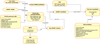Fig. 4

Flowchart summarising the selection process for new candidates included in the catalogue. A detailed description can be found in Sect. 3.2.

Table 3

eRASS start and stop times.

4.2 eROSITA timing analysis: Searching for variability

4.2.1 Creation of light curves

For our most fundamental approach to analysing the time-dependent variability of our sources, we extracted light curves. Due to the observation strategy of eROSITA to create a meaningful light curve, it is essential to take into account the changing fractional exposure at all times. In addition, the presence of a large number of faint sources in our sample, combined with high background count rates resulting from the hot interstellar medium and the high source density in the LMC, led us to employ a Bayesian approach to model background and source count rates in each time bin.

The natural time bin of eROSITA is one full rotation of the satellite (four hours), also called an eROday. However, due to the scans moving over the source, the time for which a source is visible during one eROday is variable (up to 40 s). Due to the close vicinity to the SEP, the total exposure during one eRASS can add up to more than 10 ks in the NE part of the LMC and is approximately 2 ks in the central regions. To not integrate over too long times when the source is at the edges of the FOV, we chose to use 1 s bins for the initial extraction with srctool and rebin the light curve thereafter. Before rebinning, we applied a cut in fractional exposure of 0.15 (with a few exceptions noted for individual objects) to eliminate very noisy data points at the beginning and end of scans, which occur due to high off-axis angles. For rebinning, we used two different approaches. The first one was to rebin into eROdays, for which we used the temporal offset between two primary bins, defining the start of a new eROday when the offset to the previous bin exceeded 3600 s. The second rebinning pattern we used was motivated by the low count rates of many of our objects. To obtain statistically meaningful count rates, we rebinned our light curves by ensuring a minimum number of photon counts in the on-region while allowing the bin width to vary freely. By default, we set this minimum to 10. We implied that such a bin cannot extend over the end of a period. If the last bin of a period did not have a sufficient number of photon counts, it was merged with the previous bin. The only exception to merging was when the bin was the first of its period, in which case the period was treated as a single time bin, even if it did not meet the minimum photon count threshold. In addition, we did not allow a time bin to end during an eROday. This was motivated by the large time gap between eROdays relative to their length, leading to count rates that are expected to vary more between eROdays than within a single scan.

Rebinning the light curves by a minimum number of photon counts can wash out flares for faint objects, which is why we create both types of light curves – binned by scans and binned by counts – for all of our objects.

Once the light curves were rebinned, we fitted for count rates in each new time bin using the

CmdStanPy

interface⁷ to

Stan

(Stan Development Team 2024) for using Bayesian inference. For this, we assume a constant count rate in each new bin, respectively, and assume that counts in the on- and off-region are drawn as Poisson variables as follows:

\begin{array}{l} n_{on, i} ~ Poisson ((s r c + b k g) \cdot d t_{i} \cdot f_{E, i}) \\ n_{off, i} ~ Poisson (\frac{b k g}{r_{i}} \cdot d t_{i} \cdot f_{E, i}), \end{array}

$Mathematical equation: $\eqalign{ & {n_{{\rm{on}},{\rm{i}}}}\~{\mathop{\rm Poisson}\nolimits} \left( {(src + bkg) \cdot {\rm{d}}{t_{\rm{i}}} \cdot {f_{{\rm{E}},{\rm{i}}}}} \right) \cr & {n_{{\rm{off}},{\rm{i}}}}\~{\mathop{\rm Poisson}\nolimits} \left( {{{bkg} \over {{r_{\rm{i}}}}} \cdot {\rm{d}}{t_{\rm{i}}} \cdot {f_{{\rm{E}},{\rm{i}}}}} \right), \cr} $$ (1)

where n_on,i and n_off,i are the number of photon counts in the on and off-region, respectively, src and bkg are the count rates of the source and background in the on-region which are fit for, dt_i is the time interval of an initial time bin, f_E,i are the fractional exposures and r_i is the factor by which the background counts should be scaled in order to estimate the number of background counts within the on-region. The subscript i refers to the initial time bins that are included in the new bin. We note that the criterion mentioned for rebinning to a minimum of 10 counts can be written as ∑_i n_on,i ≥ 10. We used a log-uniform prior for the source and background count rates. As uncertainties, we show the 1 σ percentiles of the source and background count rate posterior distributions in each time bin.

4.2.2 Variability

As a measure to quantify the variability of our sources and compare them to the spectrally similar AGN, we used the ratio, var, of the maximum and the minimum measured count rates as $v a r = \frac{s r c_{max}}{s r c_{min}},$ $Mathematical equation: $var = {{sr{c_{{\rm{max}}}}} \over {sr{c_{{\rm{min}}}}}},$$ (2)

where src and σ are the source count rates and corresponding uncertainties at the bins where src − σ has its maximum and where src + σ has its minimum (subscripts ‘max’ and ‘min’, respectively). We used these definitions of maximum and minimum values to avoid being dominated by high-uncertainty values. We calculated this value for light curves extracted as explained in Sects. 4.2.1 and 5.4.2.

4.2.3 Bayesian blocks

Bayesian blocks (Scargle 1998; Scargle et al. 2013a,b) is an algorithm to find change points in binned data or a list of photon arrival times. Bayesian blocks decides whether to put a change point or not based on Bayesian model comparison. The most fundamental application of Bayesian blocks is to use it to analyse count light curves or a list of arrival times without any predefined binning. However, as is mentioned in Sect. 2.1, due to the scanning procedure of eROSITA, the fractional exposure of a source changes during an observation. This means that one cannot directly compare the number of counts in different time bins; however, it is necessary to extract the corresponding count rates. Another difficulty for the standard Bayesian blocks algorithm is that, especially for fainter sources, the background is not negligible. A modification of the Bayesian blocks algorithm to incorporate those two aspects would be desirable, but this is beyond the scope of this work. Instead, we used the Gaussian Bayesian blocks implementation by

astropy

(Astropy Collaboration 2013; Astropy Collaboration 2018, 2022), which allows for the application of Bayesian blocks on a sequence of (non-integer) measured data points with Gaussian errors. For this, we used the extracted light curve as explained in Sect. 4.2.1. Due to the method we used for extracting our light curves, we typically do not find Gaussian or symmetric errors. As an estimator for the Bayesian blocks algorithm, we used the maximum of the upper and lower value at each data point and cap the value by the count rate in the given bin, such that src − σ ≥ 0. We then applied the

astropy

Bayesian blocks algorithm (

bayesian_blocks

) with the

fitness

parameter set to ‘measures’ and the false alarm probability parameter, p₀, set to 0.05. We want to note that p₀ does not exactly correspond to a probability due to several reasons:

p₀ enters the Bayesian blocks algorithm by modifying the prior for the number of changing points as a function of the number of initial bins N. Scargle et al. (2013a) did extensive simulations for binned event data and this way determined the prior as a function of N and p₀ empirically as $n c p_p r i o r = 4 - \log (73.53 p_{0} N^{- 0.478}) .$ $Mathematical equation: $ncp\_prior = 4 - \log \left( {73.53{p_0}{N^{ - 0.478}}} \right).$$ (3)

Note the correction done by Scargle et al. (2013b). This prior was developed for event data only, and it does not match the relation Scargle et al. (2013a) find for point measures done for p₀ = 0.05.
In the case of event data in the
```
astropy
```
package, there is a note that p₀ does not seem to accurately represent the false alarm probability. While the same functional form is used for ncp_prior for all three cases, there is no such comment for the case of point measures.
As was mentioned earlier, our data does not exhibit Gaussian errors, and we are forced to apply an estimation so we can use the Bayesian blocks algorithm.

For these reasons, we refrain from stating a false alarm probability of 5%. Instead, p₀ should be understood only as a parameter in our analysis. However, since we did not use Bayesian blocks to measure the variability of our sources but only as a tool to look for outbursts or flares that could otherwise be missed, this was sufficient for our needs, and we could tune the p₀ parameters using a select number of objects for which we knew which behaviour to expect.

4.2.4 Hardness ratio light curves

Drastic variability in flux in HMXB arise from variations in accretion rate and geometry, often causing spectral changes (Reig & Nespoli 2013). For example, in addition to Compton up-scattering at the accretion column, at higher accretion rates, photons can be produced through blackbody-like emission in a newly formed accretion disc. Meanwhile, cold, dense material surrounding the compact object make the spectrum appear harder through absorption.

To study these effects, we analysed spectral changes using hardness ratio (HR) light curves. We extracted 1 s binned light curves in three energy ranges: a reference band (0.2−5.0 keV; same as the band for spectral fitting) used for fractional exposure cuts, a soft band (0.2−2.0 keV), and a hard band (2.0−5.0 keV). The bands were chosen to highlight absorption effects in the soft band while ensuring a sufficient number of photons in the hard band for sources with expected power-law spectra. For better statistics, we then rebinned the data such that each new bin fulfilled two criteria:

The number of counts in the full band had to be at least 10.
The number of counts in each of the sub-bands had to be at least 1 (for higher time resolution) or 10 (for better statistics).

We then applied Eq. (1) for the soft and hard bands simultaneously to fit for the count rates and calculate the HR as $H R = \frac{s r c_{hard} - s r c_{soft}}{s r c_{hard} + s r c_{soft}} .$ $Mathematical equation: $HR = {{sr{c_{{\rm{hard}}}} - sr{c_{{\rm{soft}}}}} \over {sr{c_{{\rm{hard}}}} + sr{c_{{\rm{soft}}}}}}.$$ (4)

As uncertainties, we again used the 1σ percentiles of the posterior distribution.

4.3 Spectral fitting of the eROSITA data

4.3.1 BXA

For the spectral analysis of our sources, we used Bayesian X-ray analysis (

BXA

; Buchner 2021a).

BXA

allows one to use X-ray models from

Xspec

(Arnaud 1996) together with nested sampling from

UltraNest

(Buchner 2021b) to explore the entire model parameter space. This provides a computationally efficient tool for an unsupervised search of the best estimate parameters, utilising the Bayesian theorem.

4.3.2 Models and priors used

Most of our sources are well described by an absorbed power law (

powerlaw

Xspec

), a black body (

bbodyrad

), or a combination of the two. The power-law model is commonly used for Comptonised thermal emission in HMXBs. The blackbody emission typically originates in the accretion disc or appears on the polar cap or the surface of supersoft sources (SSSs), such as binary systems of Be stars with white dwarfs (Be/WD). For absorption, we used a

tbabs

component to account for MW foreground absorption. We used the weighted average value from Dickey & Lockman (1990) as a reference and scaled it up by a factor of 1.25 to account for the minimum contribution to absorption by molecular gas as suggested in Willingale et al. (2013). If it improved the fit, we added a

tbvarabs

model for local absorption with LMC metallicity (elemental abundances fixes at 0.49; Rolleston et al. 2002; Luck et al. 1998) if needed or a

tbpcf

component to account for partially covered sources. For all absorption models, we used abundances from Wilms et al. (2000).

For the background spectrum, we used a principal component analysis (PCA) model provided by

BXA

and fit the source and background spectra simultaneously. To determine the spectral shape of the PCA component, we first fit the off-region spectrum alone. We then kept the shape frozen and fitted the normalisation simultaneously to the off-region and, together with the source model, to the on-region, while tying the normalisations in the two regions to one another using the

BACKSCAL

value as a factor.

BACKSCAL

is the keyword calculated by

srctool

, which links the sizes of the on- and off-regions with one another.

The final important component for our models was the priors we used for the fit parameters. These are described in Table 4.

Table 4

Model priors for the spectral fits.

4.4 Investigating the variability of the optical counterpart through OGLE

We used OGLE I-band light curves to investigate the long-term variability of our sources and to search for orbital periods of the (candidate) HMXB systems. In Table D.1 we present OGLE information about the optical counterparts. While we focus on new systems or systems without published OGLE data (OGLE-IDs are listed in Table D.1), we provide references for already published OGLE data. In three cases, stars are placed near CCD gaps, which can lead to fewer measurements (indicated by the letter ‘D’ in the OGLE-IDs). For systems which show high variability in their I-band light curves (>0.3 mag), we used V-band data to investigate colour-magnitude diagrams. V-band data can be identified by the letter ‘v’ in their OGLE-IDs.

Our Fig. D.2 and Fig. D.1 in Kaltenbrunner (2025) (see Fig. D.1 for an example) present OGLE light curves of the systems investigated in this work. I- and V-band light curves are only presented for highly variable cases (>0.3 mag in I). For the latter, we created colour (V − I) magnitude (I) diagrams, as is described, for example, in Haberl et al. (2022) and shown in Fig. D.2.

To search for periodic variations in the OGLE I-band light curves, we used the Lomb-Scargle (LS) periodogram analysis (Lomb 1976; Scargle 1982), implemented in the

astropy

package of

Python

⁸. As applied to new LMC HMXBs in the past (e.g. Haberl et al. 2022, 2023), we first removed long-term trends from the light curves by subtracting a smoothed version of the light curve. To avoid false positive signals and remove true signals, we used two different methods of smoothing: applying 1) a Savitzky–Golay filter with different window lengths (Savitzky & Golay 1964) and 2) a spline fit (rspline from

wotan

; Hippke et al. 2019) with a window of 200 and a break tolerance of 500 (see Treiber et al. 2025, for an analysis of BeXRBs in the SMC). Candidate periods, which could indicate the orbital period of the binary system, are only accepted when found by both methods. In addition, we created LS periodograms from the light-curve window functions. Strong peaks are only found at 1 d, ∼0.5 year, ∼1 year, and beyond several years.

We produce LS periodograms for the three period ranges 2−20 days, 20−200 days, and 200 days to one third of the total observing time for the original and both sets of detrended light curves. The split into three period ranges allows for individual scalings, providing better visualisation of peaks with different heights. When significant peaks were found near 2 days, we also looked at shorter periods to check for aliasing effects with the sampling period of 1 day and/or short periods, which most likely are caused by non-radial pulsations (NRPs) of the Be star (e.g. Rivinius et al. 2003).

An example for the period analysis is shown in Fig. 5 for 1eRASS J054242.7−672752. While various peaks appear in the periodograms at periods longer than 20 s, a highly significant pair of sharp peaks is consistently found around 6.5 s across the different detrending methods. We newly detect periods from eleven systems, seven of which are new HMXB candidates discovered during eRASS1. The periods are listed in Table D.1, marked with ‘(TW)’, and we provide additional information on individual systems in the following.

Table 5

Known and candidate HMXB detected during eRASS1.

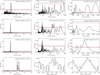Fig. 5

LS analysis of the OGLE I-band light curve of 1eRASS J054242.7−672752 (see source 46 in Table 5 and Fig. D.2). The top three rows show the LS periodogram split into three period ranges (for better visualisation): 2−20 d, 20−200 d, and 200 d to ∼1600 d, which is one-third of the monitoring period. The first row pertains to the original, the second row to the spline fit, and the third to the Savitzky–Golay filtered light curves (window 101). The bottom row shows a zoom of the LS periodogram and the light curves folded with the period with the highest power at 6.49 d (middle panel for original and right panel for spline-detrended light curves). The dashed red and black lines mark the 95 and 99% confidence levels.

4.5 Spectroscopic follow-up of optical counterparts

To securely identify the optical counterpart of our sources as Be stars, we used flux-calibrated spectra obtained using SALT, LCO/FLOYDS, and VLT FLAMES/GIRAFFE. For all three instruments, we analysed the Balmer series Hα and Hβ lines; for SALT, we additionally fitted the HeI 4921 line. Depending on the spectrum, we fitted a single- or double-peaked Gaussian or a Lorentzian line profile to the locally normalised spectrum. From the position of the line, we extracted the radial velocity with respect to the MW to verify LMC membership (radial velocity of LMC with respect to the Sun: 278±2 km s⁻¹, Richter et al. 1987). For a double-peaked line, we used the average velocity of the two lines as a reference. We determined all parameter uncertainties through Monte Carlo simulations, assuming the deviations in the line-less part of the fitted spectra are stochastic in nature. The Hα emission line profile allows us to constrain the disc inclination towards the line of sight (Hanuschik et al. 1988) and the equivalent width can be related to the size of the decretion disc (Grundstrom & Gies 2006).

4.6 SED fitting

As an additional tool to evaluate the credibility of candidates, we tested whether their archival broadband SEDs are consistent with those of a Be star. We used publicly available data from VizieR as explained in Sect. 2.7. The fitting procedure was adapted from the one described in Bodensteiner et al. (2023), where more details can be found.

The synthetic SEDs were taken from the TLUSTY OSTAR2002 and BSTAR2006 grid (Lanz & Hubeny 2003, 2007) assuming LMC metallicity. Here, we selected a constant log g of 4 (given that the SED is not directly sensitive to the surface gravity) and varied the effective temperature over all available models (that is, between 15 000 and 50 000 K). The TLUSTY models provide Eddington flux at the stellar surface, which we converted to the observed flux by scaling for the LMC distance of d =49.59 kpc (Pietrzyński et al. 2019), the stellar radius, and interstellar extinction. We varied the radius from 2 to 80 solar radii, typical of OB MS stars and supergiants (SGs). For the extinction, we used the extinction map from Skowron et al. (2021) to obtain an overall reddening value E(V−I) at the position of the star, which we converted to E(B−V) following E(V − I) = 1.237E(B − V) as indicated by the authors. To account for local variations in reddening, we treated the extinction as a free parameter, allowing it to vary between half and twice the value indicated in the extinction map. We further assume the extinction model from Gordon et al. (2023) and a constant R_V = 3.5. The IR excess is a well-known signature of the Be disc (e.g. de Wit et al. 2006), while it can also result from X-ray irradiation during major outbursts (Vasilopoulos 2025). To reduce potential contamination from the Be disc, we limited our analysis to photometric data at wavelengths below 10 microns, where its contribution is comparatively weaker.

For each model, we finally obtained the observed flux by convolving it with the corresponding filter transmission curves (Rodrigo et al. 2012; Rodrigo & Solano 2020). To find the best-fit model, we computed an overall χ² for all observation-model pairs and located the minimum. We then assessed the quality of fit to determine whether the observations can be well reproduced by an early-type star located at the LMC distance.

5 Catalogue results

Our final catalogue comprises 53 objects that meet our selection criteria (with relaxed criteria for previously known objects) and are not classified as spurious, foreground, or background sources. Among these, we detect 28 of the 59 HMXBs known prior to our study. The large number of non-detected known HMXBs can be attributed to their high intrinsic variability and the fact that they fall below eROSITA’s detection threshold. Additionally, we identify 25 candidate HMXBs, 21 of which were detected with eROSITA for the first time. One known HMXB and two candidate HMXBs were added based on their 3B detection; they would not have been included in our final catalogue had we relied solely on the eRASS1 1B catalogue (see Table 5 for details).

Of the 53 objects in our catalogue, 38 meet all the criteria required for new candidates. Given a total of 88 objects that satisfy the selection criteria for either the MCPS or VMC catalogue and an expected contamination rate of 67 ± 8% due to chance coincidences, we anticipate approximately 11 misidentified objects in our catalogue. Later in this section, we define a classification scheme into confidence classes based on optical and X-ray properties for all objects in our catalogue. With this scheme, 11 objects fall into our lowest confidence class, suggesting that the remaining catalogue has a high level of purity.

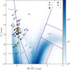Fig. 6

Gaia colour-magnitude diagram for objects in our catalogue labelled by confidence classes compared to the distribution of LMC stars (colour mesh) selected by proper motions and with overlaid contours for different stellar types (proper motion selection and stellar evolutionary phases from Gaia Collaboration (2021) evolutionary phases in Sect. 2.3.1 and figure 2; Young 1: very young main sequence (age < 50 Myr), Young 2: young main sequence (50 Myr < age < 400 Myr), BL: blue loop, RGB: red giant branch, AGB: asymptotic giant branch). The colour scale of the colour mesh gives the number of sources in each colour-magnitude bin. The bin sizes are 0.01 mag and 0.02 mag for BP−RP and G, respectively. Note that the majority of objects from confidence classes 1−5 lie in or close to the area of very young main-sequence stars, which is to be expected for Be stars. Several objects of confidence class 6 deviate strongly from this, which might indicate misidentifications.

5.1 Gaia colours

Figure 6 shows the distribution of the Gaia counterparts of objects in the catalogue compared to the entire proper motion selected sample of Gaia sources in the LMC as described in Gaia Collaboration (2021). Coloured lines separate regions in the diagram, populated by different stellar types, as shown in Fig. 2 of that work. The vast majority of objects from confidence classes 1−5 lie in or close to the area of very young main-sequence stars, which is to be expected for Be stars and SGs. Several objects of the confidence class 6 deviate strongly from this, which might indicate misidentifications.

5.2 IR colours

Similar to the SED after photometric fitting (see Sect. 4.6), the IR excess caused by the Be disc can also be observed via IR colours. Bonanos et al. (2010) used Spitzer IRAC fluxes at 3.6, 4.5, 5.8 and 8.0 µm relative to J magnitudes and found that Be stars typically exhibit high values in the IR colour J-[3.6]. They further define a photometric Be star classification for objects with J-[3.6]>0.5. Figure 7 shows IR colours for the objects in our catalogue. Remarkably, a large portion of confidence class 6 objects fall in the bottom left corner of the J over J-[3.6] plot. This corresponds to fainter and bluer objects, hinting at possible misidentifications.

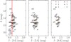Fig. 7

2MASS J magnitudes over SAGE IR colours for objects in our catalogue labelled by confidence classes. #42 stands out due to its high luminosity, caused by the SG nature of its optical companion. The notable clustering of confidence class 6 objects at the bottom left in the left figure, which accounts for their faint nature without hints of any IR excess, can be seen as an indication of misidentification of those objects. Objects missing in one or several of the plots are caused by a lack of entries in the corresponding SAGE bands.

5.3 Optical colour-colour distribution

To test the similarity of Be stars among each other, we used the plots shown in Fig. 8, which display the colour V−I over the reddening-free Q parameter (Q = U − B − 0.72 × (B − V); see Straizys et al. 1998; Aidelman & Cidale 2023). The striking difference between the LMC and SMC populations is evident in Be stars within HMXB systems, as well as in the entire Be population. The significantly higher spread observed for the LMC population suggests a greater variety in the physical properties of Be stars therein.

5.4 X-ray variability

A defining aspect of HMXB is their variability in X-ray brightness, which can be attributed to changes in accretion. This variability manifests itself both in the short and long terms.

5.4.1 Short-term

We define short-term variability as one observable over the span of the two years during which objects were observed by eROSITA. Figure 9 shows the distribution of vars (see Sect. 4.2.2) we find for 0.2−5.0 keV light curves using time bins with a minimum of 10 net counts per time bin. We compare the distributions for secure HMXB (class I, see Table 7) with candidates of different confidence levels and the same set of AGN as described in Sect. 5.5. We find that the distributions of variability in HMXBs and AGN show large similarities, with the exception that very high values of variability are predominantly observed in HMXBs. We therefore give objects with a short-term var of >100 a positive flag, indicating a high chance of being an HMXB.

5.4.2 Long-term

To study long-term variability, we used data available on the HILIGT upper limit server for XMM-Newton (slew and pointed), ROSAT (pointed and survey) and Swift and included data points for the average flux in each eRASS. Lacking knowledge of spectral changes of objects during observations included in the upper limit server, we used an absorbed power-law spectral model with a power-law index of 1 and N_H of 3×10²⁰ cm⁻² for the flux normalisation, also applying this to eROSITA data points for comparability. If the lowest flux point in the long-term light curve is an upper limit, the resulting var is a lower limit. Similar to short-term variability, we find that large values of variability are predominantly observed in HMXBs. For long-term variability, this corresponds to values greater than 30, which matches those of earlier works (Haberl & Sturm 2016). The individual long-term LCs with var values for each source are shown in Fig. A.3 in Kaltenbrunner (2025), an example can be seen in Fig. A.3.

5.5 X-ray hardness ratios

As a qualitative measure of the spectral differences between HMXBs and AGNs − our main expected contributors to misidentifications caused by chance-coincidence matches − X-ray HRs can be used. For this purpose, we used four energy bands (1: 0.2−0.5 keV, 2: 0.5−1.0 keV, 3: 1.0−2.0 keV, 4: 2.0−5.0 keV) and defined the HR as $H R_{i} = \frac{r_{i + 1} - r_{i}}{r_{i + 1} + r_{i}}$ $Mathematical equation: $H{R_i} = {{{r_{i + 1}} - {r_i}} \over {{r_{i + 1}} + {r_i}}}$$

and uncertainties as $H R_e r r_{i} = 2 \frac{\sqrt{{(r_{i} * r_e r r_{i + 1})}^{2} + {(r_{i + 1} * r_e r r_{i})}^{2}}}{{(r_{i} + r_{i + 1})}^{2}},$ $Mathematical equation: $HR\_er{r_i} = 2{{\sqrt {{{\left( {{r_i}*r\_er{r_{i + 1}}} \right)}^2} + {{\left( {{r_{i + 1}}*r\_er{r_i}} \right)}^2}} } \over {{{\left( {{r_i} + {r_{i + 1}}} \right)}^2}}},$$

where r_i is the eROSITA count rate of energy band i and r_err_i is the corresponding uncertainty. We used the values given in the forced photometry catalogue (Merloni et al. 2024).

Figure 10 shows the distribution of objects in our catalogue compared to eROSITA counterparts of known AGN. To obtain a highly clean AGN sample, we matched objects in Kozłowski et al. (2013) with known redshifts and of classes QSO-Aa or QSO-Ba with the eRASS 1 catalogue in the LMC region and maximum separations of 2^′′, minimising chance-coincidence matches. This results in a list of 61 AGN, which is comparable to the number of objects in our catalogue. One can clearly see two distributions, but the large overlap between the two distributions and the large uncertainties prevent a clear discrimination between the two groups.

Three objects that clearly stand out are located at the bottom left of the HR diagrams, which correspond to the softest sources observed. Those three objects are the Be/WD candidates, well explained by soft blackbody emitters with no detection above 2 keV (see Sect. 7.2.4).

5.6 Filtering of HMXB candidates

Candidate systems presented in this catalogue were found by matching the positions of early-type LMC stars with positions of detected X-ray sources. Despite cleaning the X-ray catalogue for known fore- and background sources (see Table 2), the high source density in the LMC paired with the size of typical X-ray error circles in the eRASS1 catalogue bears the risk of a large number of chance-coincidence matches. This would lead to a high fraction of mis-identifications without adequate filtering.

To assess the credibility of candidates, we used a combination of various properties in multiple wavelengths. We then assigned positive and negative flags and divide objects into different classes of confidence, applying an approach similar to Haberl & Sturm (2016). Table 6 lists all flags we used to rate candidates. Table 7 assigns confidence classes according to the presence of these flags and shows the number of objects in each class.

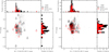Fig. 8

V−I over Q plotted for the optical companion stars in (candidate) HMXBs (black circles) and HMXBs with X-ray pulsar (red circles) as detected during eRASS1 in the LMC (left, labelled by source number from Table 5). Be stars (V<18 mag) from the list of Sabogal et al. (2005) are marked as faint grey dots. For comparison, the same is plotted for the SMC (right, source numbers from Haberl & Sturm 2016 and Be stars from Mennickent et al. 2002). The larger spread in the LMC compared to the SMC is evident in all systems.

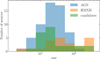Fig. 9

Short-term variability of AGN, HMXBs, and HMXB candidates represented by their var. For readability, the plot is capped at a maximum variability of 400. Six additional HMXBs exceed this var threshold, while no AGN or HMXB candidates show larger values.

5.7 Rejected HMXB candidates

The improved sensitivity and positional accuracy of eROSITA allow us to re-evaluate HMXB candidates from older surveys, such as those detected by ROSAT. In particular, we can now test whether the X-ray source positions align with early-type stars, which are the optical counterparts expected for HMXBs. If an X-ray source detected by eROSITA does not match the position of an early-type star, we can confidently reject it as an HMXB candidate, assuming that the two X-ray detections correspond to the same source. In our study, we identified five HMXB candidates, originally reported by Haberl & Pietsch (1999a) and listed in the catalogue of HMXBs in the Magellanic Clouds of Liu et al. (2005), which can now be ruled out with high confidence as HMXB candidates. This demonstrates the capability of eROSITA to refine and update earlier catalogues by improved positional uncertainties. In Table 8, a summary of the five X-ray sources can be found.

6 The X-ray luminosity function

To study the luminosity distribution of HMXBs in the LMC and to compare the population of that in the MW, SMC, and other galaxies in the local Universe with a large variety in underlying conditions, we extracted the X-ray luminosity function (XLF) of HMXBs. As was shown by Grimm et al. (2003), there is a close correlation between the recent SFR and the HMXB XLF. Close to the SEP, eROSITA allows us to probe the LMC HMXB XLF down to luminosities of ≈10³⁴ erg s⁻¹ at a completeness of 10% (see Fig. 12). However, due to eROSITA’s scanning scheme, the sensitivity is highly dependent on the position within the LMC (see Figs. 1 and 12). In order to correct our XLF for completeness, we binned our sources by luminosity and eROSITA sky tile (see Sect. 4.1 in Merloni et al. 2024). We modelled the number of sources in each luminosity bin by assuming a homogeneous source distribution throughout the LMC, that the observed number of objects is a Poisson variable, and that the detection probability equals the average sensitivity in the luminosity bin.

The luminosities we obtained by scaling the eRASS1 count rates assuming an absorbed power-law model with N_H = 6×10²⁰ cm⁻² and Γ =1. For comparison with other works in the literature, we also calculated the expected flux in the 2−12 keV range and created the corresponding XLF. Note that this should be viewed as an extrapolation and interpreted with caution. We only include objects from confidence classes 1−5 to minimise the impact of possible source contamination. Additionally, we exclude Swift J045558.9−702001, RX J0501.6−7034, 3XMM J051259.8−682640, RX J0520.5−6932, RX J0535.0−6700, RX J0544.1−7100, 4XMM J053449.0−694338, 1eRASS J054422.3−672729, and 1eRASS J055849.9−675220 from the analysis, because they would not have been included in the catalogue using the eRASS1 1B catalogue alone (see Table 5 for details). Furthermore, eRASSU J050213.8−674620, 1eRASS J050705.9−652149 and 1eRASS J054242.7−672752 were excluded due to their likely Be/WD nature, which is not typically included in the study of HMXB populations. We extracted a second luminosity function using only HMXBs of high confidence (confidence classes 1 and 2).

Figure 11 shows the results of the XLF fit. Assuming a power-law distribution of luminosities (0.2−12 keV), we followed Crawford et al. (1970) to fit an unbinned power-law function and find power-law indices of ${0.34}_{- 2.94}^{+ 0.14}$ $Mathematical equation: $0.34_{ - 2.94}^{ + 0.14}$$ and ${0.55}_{- 0.11}^{+ 0.53}$ $Mathematical equation: $0.55_{ - 0.11}^{ + 0.53}$$ , using confidence classes 1 and 2 and 1−5, respectively. Those results are similar to what Grimm et al. (2003) find as a universal value for nearby galaxies (note that the power-law indices we find are lower by 1, due to the change in the y axis). The small difference might be caused by including objects down to luminosities approximately one order of magnitude lower than Grimm et al. (2003) and a possible change in power-law index at lower luminosities, as was already suggested by Shtykovskiy & Gilfanov (2005b).

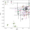Fig. 10

Hardness ratio diagram of eROSITA detections of HMXBs and HMXB candidates compared to contours showing where the eRASS counterparts of AGN in Kozłowski et al. (2013) with maximum separations of 2^′′ lie, for which 1, 2 and 3σ contours of the entire sample are plotted. The large error bars of fainter sources make a spectral identifi-cation through HR alone impossible. We identify objects #35, #37, and #46 as Be/WD candidates with spectra fit best by absorbed blackbody spectra (see Sect. 7.2.4).

Table 6

Identification flags.

Table 7

Confidence classes.

7 Discussion

7.1 X-ray luminosity function

To test the correlation between the luminosity function and the LMC SFR, we needed the luminosity function normalisation, which we obtained from an additional fit. For this purpose, we fitted a straight line in the log-log plane of Figure 11 to the binned luminosity function, freezing the slope of the line to the power-law indices we obtain with the unbinned fit. Using this fit, we could then estimate the expected number of objects with luminosities >2×10³⁸ erg s⁻¹, which is the value used by Grimm et al. (2003) to relate SFR and the HMXB population of galaxies, using the Antennae Galaxies as a reference. By then scaling this number by a factor of SRF_Antennae/N(L > 2×10³⁸ erg s⁻¹)_Antennae we get an estimate for the SFR of the LMC given its HMXB population, which we calculate as $({0.21}_{- 0.05}^{+ 0.07}) M_{⊙} {yr}^{- 1}$ $Mathematical equation: $\left( {0.21_{ - 0.05}^{ + 0.07}} \right){{\rm{M}}_ \odot }{\rm{y}}{{\rm{r}}^{ - 1}}$$ and $({0.22}_{- 0.07}^{+ 0.06}) M_{⊙} {yr}^{- 1}$ $Mathematical equation: $\left( {0.22_{ - 0.07}^{ + 0.06}} \right){{\rm{M}}_ \odot }{\rm{y}}{{\rm{r}}^{ - 1}}$$ for confidence classes 1 and 2 and 1−5, respectively. Both values match the 0.2 M_⊙yr⁻¹ found by Harris & Zaritsky (2009) using photometric MCPS data. Estimating the SFR from the HMXB luminosity function is inherently limited by the stochastic variability of the instantaneous HMXB sample size and the fact that the HMXB population reflects the SFR from several tens of millions of years in the past. This is further supported by Grimm et al. (2003), who found that the luminosity functions of the galaxies in their sample vary by a factor of ∼2 when scaled with the SFR. Given these limitations, this analysis serves as an initial step towards linking HMXBs to the LMC SFH, a connection that we shall explore in detail in our next work.

Table 8

Rejected HMXB candidates.

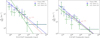Fig. 11

X-ray luminosity functions of HMXB detected during eRASS1. Green and blue points mark the expected number of sources per dex. A Poisson distribution of measured numbers is assumed. The blue and green lines mark the best-fit power-law correlation for the luminosity functions of confidence classes 1−5 and 1 and 2, respectively. The red line marks the universal power-law correlation found by Grimm et al. (2003). Left: HMXB XLF in the detection band of the eRASS1 catalogue scaling catalogue count rates assuming an absorbed power-law model with N_H = 6×10²⁰ cm⁻² and Γ = 1. Right: extrapolation to 2−12 keV range.

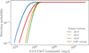Fig. 12

Sensitivity function for eRASS 1 detection assuming a spectra defined by an absorbed power-law with power-law index 1 for three positions within the LMC (sky tile closest to SEP, sky tile in the centre of the LMC and sky tile most distant from the SEP) as well as the LMC average sensitivity.

7.2 Subpopulations of HMXBs

In this section, we discuss our analysis of (groups of) objects outstanding in their multi-wavelength properties and due to follow-up observations we conducted. eROSITA timing and spectral analysis for all objects are based on Sects. 4.2 and 4.3, respectively; optical spectra use the methods described in Sect. 4.5.

7.2.1 BeXRBs detected in outburst during eRASS1

RX J0529.8−6556 is a BeXRB pulsar that was first discovered in ROSAT data (Haberl et al. 1997) with a pulse period of 69.5 s and at a flux of 3.8×10⁻¹² erg cm⁻² s⁻¹ (0.1−2.4 keV). During a deep XMM-Newton observation (Haberl et al. 2003) the source was found at a flux of 2.2×10⁻¹³ erg cm⁻² s⁻¹ (0.2−10 keV). eROSITA detected RX J0529.8−6556 in outburst (Haberl et al. 2020d) at a flux of 2.6×10⁻¹¹ erg cm⁻² s⁻¹ (0.3−8 keV) and Treiber et al. (2021) conducted targeted NICER observations to characterise the outburst. Additionally, they studied the optical behaviour using SALT spectroscopy and the 10-year OGLE V- and I-band light curves. The eROSITA spectrum is fit best with an absorbed combination of a power-law and a blackbody (

tbabs*(pow+bbodyrad)

Xspec

). No additional absorption component to account for absorption in the LMC is necessary (note that we always use a component to account for MW foreground absorption as described in Sect. 4.3). For the power law, we find an index of 0.98±0.04. The blackbody component shows a temperature of

73_{- 21}^{+ 26} eV

$Mathematical equation: $73_{ - 21}^{ + 26}{\rm{eV}}$$ and a normalisation corresponding to an emission region of

107_{- 57}^{+ 199} km

$Mathematical equation: $107_{ - 57}^{ + 199}{\rm{km}}$$ at LMC distance. The power-law component accounts for 99.1 % of the total flux of (24.3±0.6)×10⁻¹³ erg cm⁻² s⁻¹ between 0.2 and 5 keV. During the outburst (end of eRASS1, beginning of eRASS2) we find a flux of (12.35±0.16)×10⁻¹² erg cm⁻² s⁻¹ (0.2−5 keV), corresponding to an absorption-corrected luminosity of (40.7±0.5)×10³⁵ erg s⁻¹. During all other eRASSs, the source is fainter by a factor of ∼100.

eRASSU J050810.4−660653 was discovered in a bright state during eRASS1 (Haberl et al. 2020a) and with pointed XMM-Newton observations Haberl et al. (2021, 2023) confirmed it as an HMXB pulsar with a pulse period of 40.6 s. Salganik et al. (2022) then later observed eRASSU J050810.4−660653 during an episode of enhance X-ray activity with SRG/ART-XC, Swift and NuSTAR, where an orbital period of ∼38 d was found. We find the source in a bright state during all eRASSs. In the eRASS1 catalogue, the source is listed under the name 1eRASS J050810.1−660653. The merged eROSITA spectrum is best fit with an absorbed power-law with power-law index ${0.87}_{- 0.05}^{+ 0.06}$ $Mathematical equation: $0.87_{ - 0.05}^{ + 0.06}$$ and at a flux of (3.61±0.11)×10⁻¹² erg cm⁻² s⁻¹ (0.2−5 keV). The spectrum is best fit with an additional absorption component accounting for gas in the LMC, with an absorption column of $N_{H, L M C} = ({9.9}_{- 1.8}^{+ 2.2}) \times 10^{20} {cm}^{- 2}$ $Mathematical equation: ${N_{H,LMC}} = \left( {9.9_{ - 1.8}^{ + 2.2}} \right) \times {10^{20}}{\rm{c}}{{\rm{m}}^{ - 2}}$$ . Assuming standard LMC distance the luminosity corrected for absorption is (11.8±0.3)×10³⁵ erg s⁻¹. During eRASS1 we find a flux of (15.4±0.7)×10⁻¹³ erg cm⁻² s⁻¹ (0.2−5 keV), corresponding to an absorption-corrected luminosity of (50.3±2.3)×10³⁴ erg s⁻¹. Across all eRASSs, we find a var of ∼34.

eRASSU J052914.9−662446 was discovered in a bright state during eRASS1 and confirmed as a BeXRB pulsar with a spin period of 1412 s and an orbital period of ∼151 days (Maitra et al. 2020a,b). Maitra et al. (2023b) studied the broadband spectral and timing behaviour using eROSITA, Swift and NuS-TAR data in X-rays and OGLE and SALT data in optical. In the eRASS1 catalogue, the source is listed under the name 1eRASS J052914.3−662445. Across all eRASSs, we find variability of a factor ≤4. The merged eROSITA is fit best by an absorbed power-law spectrum without an additional absorption component for the LMC. We find a power-law index of ${0.30}_{- 0.07}^{+ 0.08}$ $Mathematical equation: $0.30_{ - 0.07}^{ + 0.08}$$ and a flux of (6.2±0.4)×10⁻¹³ erg cm⁻² s⁻¹ (0.2−5 keV), which corresponds to an absorption-corrected luminosity of $({19.0}_{- 1.0}^{+ 1.1}) \times 10^{34} erg s^{- 1}$ $Mathematical equation: $\left( {19.0_{ - 1.0}^{ + 1.1}} \right) \times {10^{34}}\,{\rm{erg}}\,{{\rm{s}}^{ - 1}}$$ .

Swift J053041.9−665426 was discovered during an outburst with a luminosity of 9.7×10³⁶ erg s⁻¹ in November 2011 during a Swift observation of the LMC nova 2009B (Sturm et al. 2011a). The re-detection with higher positional accuracy during Swift follow-up observations and spectral properties of the optical counterpart led to the classification as a BeXRB candidate (Sturm et al. 2011b). Charles et al. (2011) reported variability of the optical counterpart. Vasilopoulos et al. (2013a) then confirmed Swift J053041.9−665426 as a BeXRB, detecting X-ray pulsations at ∼28.78 s and a luminosity of 5.53×10³⁵ erg s⁻¹. The source was detected in outburst at the end of eRASS1, eRASS2, and eRASS3. In each successive eRASS, the outburst appeared at progressively later scan positions, consistent with an orbital period of ∼195 d. This is in line with orbital variability (Vasilopoulos et al. 2013a). The merged eROSITA spectrum can be best fit by an absorbed power-law spectrum without an additional absorption component for the LMC. We find a power-law index of 0.63±0.05 and a flux of (11.6±0.5)×10⁻¹³ erg cm⁻² s⁻¹ (0.2−0.5 keV), which corresponds to an absorption-corrected luminosity of (35.8±1.4)×10³⁴ erg s⁻¹. During the outbursts, the source displays a luminosity of (13.6±0.4)×10³⁵ erg s⁻¹, in quiescence, the source is fainter by a factor of ∼100.

Swift J0549.7−6812 is a BeXRB system that was discovered serendipitously in 2013 with the hard X-ray transient monitor of the Swift Burst Alert Telescope (BAT, Krimm et al. 2013a). Krimm et al. (2013c) found the source to be consistent with the position of the faint ROSAT object 1RXS J055007.0−681451, which was detected at a luminosity of 6.4×10³⁴ erg s⁻¹ (assuming a typical spectral power-law index of 1). Krimm et al. (2013b) later conducted targeted Swift observations that revealed X-ray pulsations with a 6.2 s period, and associated the X-ray source with an early-type star, identifying it as an HMXB. They reported that during a deep Chandra observation (OBSID 3850; 67.5 ks on 2 October 2003), no X-ray source consistent with Swift J0549.7−6812 was detected, suggesting the source must have been fainter by a factor of at least ∼100 compared to the ROSAT observations. Coe et al. (2023) reported that the 2013 Swift observations coincided with an outburst, during which the source showed a peak luminosity of 8.1×10³⁷ erg s⁻¹ (0.3−10 keV), and that long-term Swift/BAT observations over 10 yr have not shown any additional X-ray outbursts. They also conducted SALT/RSS observations of the optical counterpart, which revealed Hα and Hβ in emission, confirming the BeXRB nature of the source. Swift J0549.7−6812 was detected in an outburst in eRASS1 at an average flux of (3.9±0.4)×10⁻¹³ erg cm⁻² s⁻¹ (0.2−5 keV), which corresponds to an absorption-corrected luminosity of (1.19±0.11)×10³⁵ erg s⁻¹. At the peak of the outburst during eRASS1, the source reached a luminosity of ∼7.0×10³⁵ erg s⁻¹ with the event lasting for ∼17 days. These characteristics are consistent with a type I outburst. The entire eROSITA light curve can be seen in Fig. 13. During all other eRASSs, the source is fainter by a factor of at least ∼10 and lies below the background flux. The merged spectrum can be best fit by an absorbed power law without an additional absorption component for the LMC. The best-fit power-law index is 0.56±0.20.

eRASSU J050213.8-674620 was first detected during an outburst in eRASS1. As a Be/WD candidate, the source is discussed in more detail in Sect. 7.2.4.

7.2.2 A population of SgXRBs

SgXRBs consist of a NS accreting from an OB SG, primarily through stellar winds or Roche-lobe overflow. They typically show persistent or moderately variable X-ray emission (10³⁵–10³⁸ erg s⁻¹; Martínez-Núñez et al. 2017) and short orbital periods of the order of a few days (Walter et al. 2015). Many SgXRBs display pulsations due to the spin of a magnetised NS, as well as eclipses and orbital modulation driven by interactions with the dense stellar wind. Some also exhibit superorbital variability.

RX J0532.5−6551 was first detected by Haberl et al. (1995). Based on the optical classification of the proposed counterpart, they classified it as an SgXRB. During the ROSAT observations between 1990 and 1994, they observed a change in flux by a factor of ∼50 with an average X-ray luminosity of a few 10³⁴ erg s⁻¹ and a maximum luminosity of 1.9×10³⁵ erg s⁻¹ (0.1−2.4 keV). Later, Negueruela & Coe (2002) and Jaxon et al. (2001) independently confirmed the SgXRB classification, and Negueruela & Coe (2002) further confirmed the system to be the first wind-fed SgXRB system known in the LMC. The merged eROSITA spectrum can best be fit by an absorbed power-law without an additional component to account for local absorption. We find a power-law index of 0.58±0.05 and a flux of (8.5± 0.3)×10⁻¹³ erg cm⁻² s⁻¹ (0.2−5 keV), corresponding to an absorption-corrected luminosity of $({2.62}_{- 0.10}^{+ 0.09}) \times 10^{35} erg s^{- 1}$ $Mathematical equation: $\left( {2.62_{ - 0.10}^{ + 0.09}} \right) \times {10^{35}}\,{\rm{erg}}\,{{\rm{s}}^{ - 1}}$$ .

LMC X−1 was the first extra-galactic HMXB to be detected (Mark et al. 1969). It consists of an O-type SG, and a BH with a mass of 10.9 M_⊙ (Orosz et al. 2009). LMC X−1 is characterised by soft X-ray spectrum at a relatively constant luminosity of ∼2×10³⁸ erg s⁻¹. We fit the merged eROSITA spectrum with an absorbed disc-blackbody spectrum with an additional absorption component to account for local absorption (

tbabs

tbvarabs

diskbb

Xspec

). The best-fit parameters are

NH = ({4.91}_{- 0.17}^{+ 0.18}) \times 10^{21} {cm}^{- 2}

$Mathematical equation: ${{\rm{N}}_{\rm{H}}} = \left( {4.91_{ - 0.17}^{ + 0.18}} \right) \times {10^{21}}{\rm{c}}{{\rm{m}}^{ - 2}}$$ and

T_{in} = (800_{- 14}^{+ 15}) eV

$Mathematical equation: ${{\rm{T}}_{{\rm{in}}}} = \left( {800_{ - 14}^{ + 15}} \right){\rm{eV}}$$ at a flux of (5.22±0.07)×10⁻¹⁰ erg cm⁻² s⁻¹ (0.2−5 keV). This corresponds to an absorption-corrected luminosity of (2.42±0.03)×10³⁸ erg s⁻¹. Similar to what was observed in the past, LMC X−1 showed low variability across all eRASS, with a factor of ∼4.

LMC X−3 is another binary system of an SG filling its Roche lobe and a BH with a mass of 6.98 M_⊙ (Soria et al. 2001; Orosz et al. 2014). We fitted the merged eROSITA spectrum with an absorbed combination of a power-law and a disc-blackbody model (

tbabs

pow

diskbb

) in

Xspec

). We find a power-law index of

({1.82}_{- 0.08}^{+ 0.11})

$Mathematical equation: $(1.82_{ - 0.08}^{ + 0.11})$$ and a temperature of T_eff=(0.79±0.03) keV at an average flux of (7.09±0.07)×10⁻¹⁰ erg cm⁻² s⁻¹, which corresponds to an absorption-corrected luminosity of (24.94±0.24)×10³⁷ erg s⁻¹.

LMC X−4 is an eclipsing high-mass binary pulsar. An orbital solution of the binary shows a mass of 18 M_⊙ for the O-type SG and 1.57 M_⊙ for the NS (Falanga et al. 2015, and references therein). The merged eROSITA spectrum is best fit by an absorbed combination of a blackbody, a hard and a soft power-law (

tbabs

bbodyrad

pow

pow

) in

Xspec

) without an additional local absorption component. For the blackbody component we find

T_{eff} = (43_{- 3}^{+ 4}) eV

$Mathematical equation: ${T_{{\rm{eff}}}} = \left( {43_{ - 3}^{ + 4}} \right){\rm{eV}}$$ . For the soft and hard power-law components, we find α = 2.17 ± 0.05 and

α = - {1.7}_{- 0.5}^{+ 0.4}

$Mathematical equation: $\alpha = - 1.7_{ - 0.5}^{ + 0.4}$$ , respectively. The average flux during all eRASSs is (3.06±0.06)×10⁻¹¹ erg cm⁻² s⁻¹ (0.2−5 keV), which corresponds to an absorption-corrected luminosity of

({1.83}_{- 0.09}^{+ 0.10}) \times 10^{37} erg s^{- 1}

$Mathematical equation: $\left( {1.83_{ - 0.09}^{ + 0.10}} \right) \times {10^{37}}\,{\rm{erg}}\,{{\rm{s}}^{ - 1}}$$ .

XMMU J053108.3−690923, XMMU J053320.8−684122 and 1eRASS J054422.3−672729 are (candidate) systems of the sub-class of SFXTs and are discussed in Sect. 7.2.3.

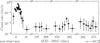Fig. 13

eROSITA light curve for the BeXRB Swift J0549.7−6812. During the outburst in eRASS1, the flux rises to a maximum of ∼3.5×10³⁵ erg s⁻¹. For readability, white spaces between the individual eRASSs are removed. The light curve is rebinned to have a minimum number of 10 net source counts per time bin as described in Sect. 4.2.1. The variability var (found in the bottom right) is calculated as described in Sect. 4.2.2.

7.2.3 Supergiant fast X-ray transients

Supergiant fast X-ray transients are a subtype of SgXRBs characterised by a faint nature during the majority of the time, interrupted by sporadic strong flares that only last for a few hours and during which the flux typically rises by a factor of a hundred or more. Often, those flares appear grouped during periods of higher activity and are accompanied by spectral changes. The exact mechanics leading to this behaviour are still a matter of debate. Plausible explanations include clumpiness of the stellar wind (in’t Zand 2005), magnetic or centrifugal gates due to the NS rotation and strong magnetic fields (Bozzo et al. 2008), as well as the onset of a long-standing settling accretion regime (Shakura et al. 2012).

In eRASS1, we detect both SFXTs in the LMC known from the literature. Additionally, find one new object that displays a typical SFXT behaviour, 1eRASS J054422.3−672729, showing an increase in flux by a factor of ∼100 and ∼50 during two flares, respectively. We propose that this should be seen as a lower limit for the variability of this system, because it is likely that the system’s brightest state was not observed due to eROSITA’s scanning scheme. Typical SFXT dynamical ranges can be up to ∼10³−10⁵ between quiescence and outburst (Romano 2015).

XMMU J053320.8−684122 was first detected by Sturm et al. (2012b) during a Swift survey and a follow-up observation in 2012, at fluxes of 5.4×10⁻¹³ erg cm⁻² s⁻¹ and 8.1×10⁻¹³ erg cm⁻² s⁻¹, respectively (Swift J053321.3−684121). It was later re-detected during observations for the XMM-Newton large survey of the LMC. Vasilopoulos et al. (2018) then conducted a detailed study of X-ray data from XMM-Newton and Swift combined with optical spectra obtained with the Fibre-fed Extended Range Optical Spectrograph (FEROS; Kaufer et al. 1999) and photometric data from the Gamma-Ray Burst Optical and Near-Infrared Detector (GROND; Greiner et al. 2008). They found a mean flux of 8.4×10⁻¹³ erg cm⁻² s⁻¹ (0.3−10 keV) with a flux increase by a factor of ∼13 towards the end of the XMM-Newton observation. Given the optical data indicating an SG companion, it is proposed that XMMU J053320.8−684122 belongs to the class of SFXTs. The eROSITA light curve shows a var of ∼120, and our Bayesian blocks analysis reveals that it stays in a quiescent state most of the time to brighten up by a factor of ∼10 for several days during eRASS1, 2 and 4. The spectrum is fit best with an absorbed power-law at a mean flux of $({3.5}_{- 0.4}^{+ 0.5}) \times 10^{- 13} erg {cm}^{- 2} s^{- 1} (0.2 - 5 keV)$ $Mathematical equation: $\left( {3.5_{ - 0.4}^{ + 0.5}} \right) \times {10^{ - 13}}{\rm{erg}}\,{\rm{c}}{{\rm{m}}^{ - 2}}{{\rm{s}}^{ - 1}}(0.2 - 5\,{\rm{keV}})$$ erg cm⁻² s⁻¹ (0.2−5 keV) with a power-law index of 0.6±0.4 and with a high local absorption of $({1.1}_{- 0.5}^{+ 0.6}) \times 10^{22} {cm}^{- 2}$ $Mathematical equation: $\left( {1.1_{ - 0.5}^{ + 0.6}} \right) \times {10^{22}}{\rm{c}}{{\rm{m}}^{ - 2}}$$ . This corresponds to an absorption-corrected luminosity of ${13.3}_{- 1.4}^{+ 1.7} \times 10^{34} erg s^{- 1}$ $Mathematical equation: $13.3_{ - 1.4}^{ + 1.7} \times {10^{34}}\,{\rm{erg}}\,{{\rm{s}}^{ - 1}}$$ .

XMMU J053108.3−690923 was first reported as an SgXRB by Vasilopoulos et al. (2018) by using optical spectroscopy for the SG classification of the optical companion. Using XMM-Newton they detected X-ray variability at a period of ∼2013 s, which is very high for typical pulsars in HMXBs. Maitra et al. (2021b) later verified the high spin period of ∼2020 s with eROSITA and XMM-Newton observations. During two of the eROSITA pointed observations, they also observed strong flares, during which the flux increased by a factor of ∼15 and ∼30, respectively, leading them to classify the system as an SFXT. Across all the eRASSs, we do not detect any significant changes in the luminosity of XMMU J053108.3−690923. The merged eROSITA spectrum is fit best by an absorbed power-law with an additional component for LMC absorption. The best-fit parameters are an absorption of $N_{H, L M C} = ({3.3}_{- 1.5}^{+ 2.0}) \times 10^{22} {cm}^{- 2}$ $Mathematical equation: ${N_{H,LMC}} = \left( {3.3_{ - 1.5}^{ + 2.0}} \right) \times {10^{22}}{\rm{c}}{{\rm{m}}^{ - 2}}$$ , a power-law index of ${0.9}_{- 0.7}^{+ 0.8}$ $Mathematical equation: $0.9_{ - 0.7}^{ + 0.8}$$ and a flux of $({2.2}_{- 0.4}^{+ 0.5}) \times 10^{- 13} erg {cm}^{- 2} s^{- 1} (0.2 - 5 keV)$ $Mathematical equation: $\left( {2.2_{ - 0.4}^{ + 0.5}} \right) \times {10^{ - 13}}{\rm{erg}}\,{\rm{c}}{{\rm{m}}^{ - 2}}{{\rm{s}}^{ - 1}}(0.2 - 5{\rm{keV}})$$ , which corresponds to an absorption-corrected luminosity of $({1.1}_{- 0.3}^{+ 0.8}) \times 10^{35} erg s^{- 1}$ $Mathematical equation: $\left( {1.1_{ - 0.3}^{ + 0.8}} \right) \times {10^{35}}{\rm{erg}}\,{{\rm{s}}^{ - 1}}$$ .

We find 1eRASS J054422.3−672729 as a new HMXB candidate in the course of this study. The optical properties of its companion match those of an SG in terms of colour and brightness. Analysis of OGLE I-band data revealed a highly significant 5.25 d period, which likely is the orbital period of the system. The source is seen in a state of increased flux twice, once during eRASS2 and once during eRASS4, where the flux increased by a factor of ∼100 and ∼50, respectively, and which each last for ∼1 d. We propose 1eRASS J054422.3−672729 as a new SFXT. The merged eROSITA spectrum can be best fit with an absorbed power law, with an additional component to account for LMC absorption. The best-fit parameters are $N_{H, L M C} = ({0.8}_{- 0.3}^{+ 0.4}) \times 10^{22} {cm}^{- 2}$ $Mathematical equation: ${N_{H,LMC}} = \left( {0.8_{ - 0.3}^{ + 0.4}} \right) \times {10^{22}}{\rm{c}}{{\rm{m}}^{ - 2}}$$ for the absorption, 2.1±0.6 for the power-law index and $({5.8}_{- 1.2}^{+ 1.5}) \times 10^{- 14} erg {cm}^{- 2} s^{- 1} (0.2 - 5 keV)$ $Mathematical equation: $\left( {5.8_{ - 1.2}^{ + 1.5}} \right) \times {10^{ - 14}}{\rm{erg}}\,{\rm{c}}{{\rm{m}}^{ - 2}}{{\rm{s}}^{ - 1}}(0.2 - 5{\rm{keV}})$$ for the flux, which corresponds to and absorption-corrected luminosity of $({4.2}_{- 1.0}^{+ 3.3}) \times 10^{34} erg s^{- 1}$ $Mathematical equation: $\left( {4.2_{ - 1.0}^{ + 3.3}} \right) \times {10^{34}}{\rm{erg}}\,{{\rm{s}}^{ - 1}}$$ . We conducted a series of ten 1200 s exposure SALT observations between 2023-11-05 and 2023-11-23 to study the optical counterpart of 1eRASS J054422.3−672729. We specifically studied the equivalent widths and kinematics of the Lyman Hα and Hβ lines, as well as those of the HeI 4921 lines. The line profiles are best fit by a wide absorption line with a narrow emission line for Hα and Hβ, and a single absorption line for HeI 4921. See Figure 16 for the normalised spectra with best-fit functions at the Hα line for all observations. Table 9 lists the best-fit parameters for the Hβ and HeI 4921 lines. We tested whether the velocity shift or the change in equivalent width could be linked to the orbital period derived from OGLE, but found no indication of such a link for any of the three lines. In the case of the HeI 4921 line, this may be due to low S/N.

The light curve of 1eRASS J054422.3−672729 can be seen in Fig. 14 in two energy bands and the HR of those two bands as defined in Eq. (4). Two flares at 373 days and 730 days are clearly visible in the soft band and are less pronounced in the hard band. The HR indicates a spectral softening of the spectrum during the flares. It is possible that this spectral softening, as opposed to the often observed hardening, is caused by low statistics during quiescence. Alternatively, the observed behaviour could resemble that of the objects in Ferrigno et al. (2022), which showed no spectral hardening. This may indicate alternative mechanisms to gas clump accretion, or that the clumps are not located along the LOS. Also, the observed dynamic ranges for all three systems observed by eROSITA should be understood as a lower limit, as eROSITA is likely to have missed the main flare due to its scanning scheme. An interesting feature we found is that both flares seem to happen at the same orbital phase, using the orbital period we found by analysing OGLE data (see Sect. 7.4). This can be seen in Fig. 15. In general, X-ray flares appear more concentrated around periastron passage in many SFXT systems (e.g. Sidoli et al. 2006; Gamen et al. 2015), which could be what is seen in 1eRASS J054422.3−672729 and agrees with the scenario of accretion from the clumpy wind of an SG. Nevertheless, flares also appear during other orbital phases (e.g. Smith et al. 2012; Goossens et al. 2013; Sidoli et al. 2023), preventing any definitive interpretation in the absence of an orbital solution.

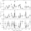Fig. 14

eROSITA light curve of 1eRASS J054422.3−672729 in the energy bands 0.2−2.0 keV (soft; top), 2.0−5.0 keV (hard; middle) and the HR defined from those two bands (bottom). The light curve is binned such that there is a minimum of 1 net count in each band and a minimum of 10 net counts in the sum of the two bands per time bin. The flares at ∼373 and ∼730 days are marked with dotted grey lines and can be best seen in the soft band. The HR light curve indicates spectral softening at those times. Note that time gaps between eRASSs are cut out for readability.

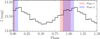Fig. 15

OGLE phase-folded light curve of 1eRASS J054422.3−672729 with timing of the flares marked. Flares 1 and 2 refer to the flares at 373 and 730 days in Fig. 14, respectively.

7.2.4 Be/WD binaries

The vast majority of HMXBs found to date consist of a Be star and an NS. This contradicts the expectations of binary evolution models, which predict that there should be a factor of seven more systems with a WD as a compact object than the number of Be/NS binaries (Pols et al. 1991; Raguzova 2001). However, to date, only a few such systems are known (Kahabka et al. 2006; Sturm et al. 2012a; Coe et al. 2020; Kennea et al. 2021a; Marino et al. 2025).

Among the candidates newly detected with eROSITA, we find three objects with spectral properties that cannot be explained by the model of a Be/NS system with a hard X-ray spectrum. All three show soft blackbody spectra with close to no or no emission above 2 keV, which is typical for SSSs (Maitra & Haberl 2022). This points towards their nature as Be systems containing a WD or BH. Be/BHs are elusive objects that are mostly expected to be X-ray faint (Sen et al. 2021). Recently, BPS models have predicted a fraction of Be/BH systems in the luminosity range of 10³¹⁻³⁵ erg s⁻¹ with a non-thermal spectrum (Sen et al. 2024).

eRASSU J050213.8−674620 was first detected during eRASS1 (Haberl et al. 2020b) and as an optical companion AL 55 (Howarth 2013), a star with typical features of an early type star, was proposed. In the eRASS1 catalogue, the source is listed under the name 1eRASS J050214.6-674616. We conducted follow-up LCO/FLOYDS observations for a spectral classification of the optical counterpart and found a strong Hα emission line of (−28.11 ± 0.22) Å, which confirms its Be nature. The line is at a radial velocity of (146.8 ± 2.0) km s⁻¹ relative to the LMC rest frame. The eROSITA spectrum is best described by an absorbed blackbody spectrum without an additional absorption component for the LMC. The best-fit temperature is $({45.8}_{- 2.1}^{+ 2.3}) eV$ $Mathematical equation: $\left( {45.8_{ - 2.1}^{ + 2.3}} \right){\rm{eV}}$$ . eRASSU J050213.8−674620 shows a flux of (6.4±0.5)×10⁻¹³ erg cm⁻² s⁻¹ (0.2−2.0 keV) during eRASS1. During all other eRASSs, the flux lies below the background flux, which requires a change of at least two orders of magnitude. Assuming LMC distance the flux during eRASS1 corresponds to an emission radius of $(2800_{- 500}^{+ 700}) km$ $Mathematical equation: $\left( {2800_{ - 500}^{ + 700}} \right){\rm{km}}$$ and an absorption-corrected luminosity of (1.52 ± 0.12)×10³⁶ erg s⁻¹. This suggests emission from the entire surface of a WD.

For the optical counterpart of 1eRASS J050705.9−652149 we find strong Hα emission of (−26.8 ± 0.4) Å at a radial velocity of (150 ± 4) km s⁻¹ relative to the LMC. It shows a higher flux during eRASS1, but in contrast to eRASSU J050213.8−674620, the flux goes down only by a factor of ∼10. We find a best-fit blackbody temperature of $(85_{- 14}^{+ 20}) eV$ $Mathematical equation: $\left( {85_{ - 14}^{ + 20}} \right){\rm{eV}}$$ . During eRASS1, we find a flux of (3.0±0.7)×10⁻¹⁴ erg cm⁻² s⁻¹, which at LMC distance corresponds to an absorption-corrected luminosity of (2.1±0.5)×10³⁴ erg s⁻¹ and an emission radius of $(63_{- 28}^{+ 54}) km$ $Mathematical equation: $\left( {63_{ - 28}^{ + 54}} \right){\rm{km}}$$ . Averaging over all eRASSs we find a flux of (9.1±2.6)×10⁻¹⁵ erg cm⁻² s⁻¹, corresponding to an absorption-corrected flux of $({6.2}_{- 2.1}^{+ 2.7}) \times 10^{33} erg s^{- 1}$ $Mathematical equation: $\left( {6.2_{ - 2.1}^{ + 2.7}} \right) \times {10^{33}}\,{\rm{erg}}\,{{\rm{s}}^{ - 1}}$$ or an emission radius of $(35_{- 16}^{+ 30}) km$ $Mathematical equation: $\left( {35_{ - 16}^{ + 30}} \right){\rm{km}}$$ , possibly originating from a hot spot on the surface of a WD.

The LCO/FLOYDS spectrum of the optical companion of 1eRASS J054242.7−672752 shows Hα at (−10.7±0.2) Å at a radial velocity of (24±8) km s⁻¹, confirming its Be nature. The eROSITA data show a constant flux across all eRASSs, which is best fit with an absorbed blackbody spectrum without an additional LMC absorption component. We find a best-fit blackbody temperature of 88 ± 6 eV and a flux of $({2.69}_{- 0.28}^{+ 0.30}) \times 10^{- 14} erg {cm}^{- 2} s^{- 1} (0.2 - 2.0 keV)$ $Mathematical equation: $\left( {2.69_{ - 0.28}^{ + 0.30}} \right) \times {10^{ - 14}}{\rm{erg}}\,{\rm{c}}{{\rm{m}}^{ - 2}}{{\rm{s}}^{ - 1}}(0.2 - 2.0\,{\rm{keV}})$$ . Assuming LMC distance, the flux corresponds to an emission radius of $(65_{- 12}^{+ 15}) km$ $Mathematical equation: $\left( {65_{ - 12}^{ + 15}} \right){\rm{km}}$$ or an absorption-corrected luminosity of $({2.4}_{- 0.3}^{+ 0.4}) \times 10^{34} erg s^{- 1}$ $Mathematical equation: $\left( {2.4_{ - 0.3}^{ + 0.4}} \right) \times {10^{34}}{\rm{erg}}\,{{\rm{s}}^{ - 1}}$$ . Similar to 1eRASS J050705.9−652149, this can be explained by emission from a hot spot on the surface of a WD.

To evaluate whether the eROSITA spectra of the three sources can be alternately explained by BH binaries, we tested two standard models. First, we applied an absorbed power-law model, allowing for local absorption and power-law indices in the range 0.0 to 4.0, using a flat prior (

tbabs*tbvarabs*pow

Xspec

). This type of model is typically associated with the low-hard state observed in BH binaries. For eRASSU J050213.8−674620, this model can be clearly rejected. In contrast, for 1eRASS J050705.9−652149 and 1eRASS J054242.7−672752, the low source flux relative to the background prevents a definitive rejection. However, in both cases, the posterior distribution for the power-law index peaks at the upper boundary of the prior, indicating a potentially even higher value. Since power-law indices observed in BH systems generally lie below ∼3, this model is also disfavoured for the two fainter sources.

The second model we tested was an absorbed multi-blackbody model (

tbabs*tbvarabs*diskbb

Xspec

), which is typically observed only in the high-soft state during periods of high accretion. The parameters were constrained within the expected range for Schwarzschild BHs with masses between 10/3 M_⊙ and 30 M_⊙, assuming a face-on accretion disc. For the inner disc radius, we adopted the innermost stable circular orbit (ISCO):

R_{ISCO} = \frac{6 G M}{c^{2}},

$Mathematical equation: ${R_{{\rm{ISCO}}}} = {{6GM} \over {{c^2}}},$$

where M is the BH mass, G the gravitational constant, and c the speed of light.

The temperature at the inner disc radius was taken as the maximum temperature in the distribution described by Shakura & Sunyaev (1973) $T_{\max} = \frac{6 \sqrt{6}}{7 \cdot 7^{3 / 4}} {(\frac{3}{8 π \cdot 6^{3}})}^{1 / 4} {(\frac{\dot{M} c^{6}}{G^{2} M^{2} σ})}^{1 / 4} \approx 0.075 {(\frac{\dot{M} c^{6}}{G^{2} M^{2} σ})}^{1 / 4},$ $Mathematical equation: ${T_{\max }} = {{6\sqrt 6 } \over {7 \cdot {7^{3/4}}}}{\left( {{3 \over {8\pi \cdot {6^3}}}} \right)^{1/4}}{\left( {{{\dot M{c^6}} \over {{G^2}{M^2}\sigma }}} \right)^{1/4}} \approx 0.075{\left( {{{\dot M{c^6}} \over {{G^2}{M^2}\sigma }}} \right)^{1/4}},$$

at $r = \frac{49}{36} R_{ISCO}$ $Mathematical equation: $r = {{49} \over {36}}{R_{{\rm{ISCO}}}}$$ , where $\dot{M}$ $Mathematical equation: $\dot M$$ is the mass accretion rate and σ is the Stefan–Boltzmann constant.

As a lower limit for the accretion rate, we adopted $\dot{M} \geq 10^{- 2} {\dot{M}}_{Edd} \approx 10^{- 10} \frac{M}{M_{⊙}} \frac{M_{⊙}}{yr}$ $Mathematical equation: $\dot M \ge {10^{ - 2}}{\dot M_{{\rm{Edd}}}} \approx {10^{ - 10}}{M \over {{M_ \odot }}}{{{M_ \odot }} \over {{\rm{yr}}}}$$ , where ${\dot{M}}_{Edd}$ $Mathematical equation: ${\dot M_{{\rm{Edd}}}}$$ is the Eddington mass accretion rate, following Esin et al. (1997), who find that accretion discs are not formed below this threshold. This model results in a poor fit and can be robustly rejected for all three sources. We therefore propose all three objects as new Be/WD candidates. Figures 17, 18 and 19 show the merged eROSITA spectra with best-fit absorbed black body models for the three sources.

Be/WDs have been relatively elusive, with only a few such systems identified, and these are usually observed during X-ray outbursts, attributed to a thermonuclear runaway. eRASSU J050213.8−674620 falls into this pattern. It is detected only during eRASS1, where the entire WD surface appears to be emitting X-rays at a temperature of ∼50 eV. In contrast, it appears that 1eRASS J054242.7−672752 and 1eRASS J050705.9−652149 are in a persistent emission state. Their spectral fits agree with temperatures of ∼100 eV and luminosities corresponding to emission regions of ∼50 km.

Given those higher blackbody temperatures and much smaller emission regions, this suggests emission from hot spots on the WD surface. Sturm et al. (2012a) observed the SSS XMMU J010147.5−715550 in the SMC in a similar state.

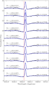Fig. 16

Hα profiles of SALT observations of the optical counterpart of 1eRASS J054422.3−672729 between 5 and 23 November 2023 shifted to the rest-frame of the LMC. The black line shows the data, the blue line shows the best-fit spectrum using a wide absorption line and a narrow emission line feature, and the dashed red line indicates the rest-frame wavelength of Hα. Between individual observations lies a shift of 1.5 for the normalised flux for readability. The equivalent widths and radial velocities are given for the narrow absorption line.

Table 9

Best-fit results for Hβ and HeI 4921 lines for SALT spectra of 1eRASS J054422.3−672729.

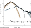Fig. 17

eROSITA spectra of the Be/WD candidate eRASSU J050213.8−674620 merged over all eRASS. Black data points represent the flux in the on-region, while blue data points represent the flux in the off-region, scaled by the size difference between the on- and off-regions. The dark yellow curve represents the best-fit model for the source (absorbed black body), and the shaded areas surrounding it indicate the 1 and 3 sigma regions for the model. The blue curve and shaded area show the best fit for the PCA background model. The black curve and shaded area are the sum of the source and background models.

Fig. 18

Same as Fig. 17 but for 1eRASS J054242.7−672752 without local absorption.

Fig. 19

Same as Fig. 17 but for 1eRASS J050705.9−652149 without local absorption.

7.2.5 Persistent BeXRBs

High-mass X-ray binaries, predominantly systems with a Be star counterpart (BeXRBs), are characterised by eccentric orbits, resulting in a transient nature. During a large portion of the orbit, the systems stay in an X-ray quiescent state until they undergo a major outburst during periastron passage.

Persistent HMXBs are so far scarcely studied sub-class of HMXBs that are characterised by relatively low luminosities of ≲10³⁴ erg s⁻¹ and a lack of major outbursts. Pfahl et al. (2002) proposed that this behaviour is caused by long orbital periods and low eccentricities. Due to their wide orbits, no tidal circu-larisation could have occurred after the supernova explosion that created the NS. Therefore, the low-eccentricity orbit must have formed in a supernova explosion without a significant kick. It was found that NSs in such systems exhibit longer spin periods of the order of a few hundred to a thousand seconds (Reig & Roche 1999; La Palombara & Mereghetti 2007; La Palombara et al. 2009, 2012). This can be explained by quasi-spherical accretion or very high magnetic fields of the NS, leading to gating mechanisms. In the subsonic regime, accretion occurs where the plasma remains hot until it reaches the magnetosphere, forming a hot, quasi-spherical shell (Shakura et al. 2012).

4XMM J053449.0−694338 is a new HMXB candidate we identified in this work. The source shows long-term variability (see Sect. 5.4.2) of a factor ∼10 over a period of 30 years. The merged eROSITA spectrum is fit best with an absorbed power-law without an additional absorption component for the LMC, a power-law index of 1.6±0.4 and a flux of $({5.0}_{- 1.4}^{+ 1.5}) \times 10^{- 14} erg {cm}^{- 2} s^{- 1}$ $Mathematical equation: $\left( {5.0_{ - 1.4}^{ + 1.5}} \right) \times {10^{ - 14}}{\rm{erg}}\,{\rm{c}}{{\rm{m}}^{ - 2}}{{\rm{s}}^{ - 1}}$$ . This corresponds to an absorption-corrected luminosity of (1.9±0.5)×10³⁴ erg s⁻¹. To study the characteristics of 4XMM J053449.0−694338 in more detail, we conducted XMM-Newton follow-up observations (obs.-ID 0943900201; obs. time: 2024-07-18 22:47 – 2024-07-19 16:34). The exposure time after background-flare screening for EPIC-pn is 40520 s. The spectral analysis was conducted on events with

PATTERN

1–4 using the conservative event filtering with

FLAG

=0. The response files were computed with the

XMMSAS

(version

xmmsas_22.1.0-a8f2c2afa-20250304

⁹) tasks

arfgen

and

rmfgen

. To optimise the S/N, we used data up to 6.0 keV for our fit. For the spectral shape of the background, we used a PCA model provided by

BXA

similar to our analysis of eROSITA data (see Sect. 4.3.2). This PCA model is fit-able only down to detector channel 41, which confines our spectral fit to energies larger than ∼0.22 keV. Our best-fit model for the source is an absorbed combination of a power-law and a blackbody with an additional absorption component to account for gas in the LMC (

tbabs*tbvarabs*(pow+bbodyrad)

Xspec

). The best-fit parameters are a power-law index of

{1.50}_{- 0.23}^{+ 0.44}

$Mathematical equation: $1.50_{ - 0.23}^{ + 0.44}$$ , an effective temperature of

{0.77}_{- 0.22}^{+ 0.21} keV

$Mathematical equation: $0.77_{ - 0.22}^{ + 0.21}{\rm{keV}}$$ and a local absorption of

({7.5}_{- 7.0}^{+ 14.1}) \times 10^{20} {cm}^{- 2}

$Mathematical equation: $\left( {7.5_{ - 7.0}^{ + 14.1}} \right) \times {10^{20}}{\rm{c}}{{\rm{m}}^{ - 2}}$$ . For the flux we find (5.2±0.4)×10⁻¹⁴ erg cm⁻² s⁻¹ (0.2–6 keV), which corresponds to a luminosity corrected for absorption of

({1.85}_{- 0.18}^{+ 0.28}) \times 10^{34} erg s^{- 1}

$Mathematical equation: $\left( {1.85_{ - 0.18}^{ + 0.28}} \right) \times {10^{34}}{\rm{erg}}\,{{\rm{s}}^{ - 1}}$$ . The blackbody normalisation corresponds to an emission region of

(340_{- 190}^{+ 160}) m

$Mathematical equation: $\left( {340_{ - 190}^{ + 160}} \right){\rm{m}}$$ and the blackbody component accounts for ∼30% of the total flux. The EPIC-pn spectrum with the best-fit model is shown in Fig. 20. Correcting the event arrival times to the Solar System barycentre, we created an EPIC-pn light curve and conducted a search for periodic variability using an LS periodogram in the range 10–1000 s. We do not find any significant periodicity in the data.

Similarly, 4XMM J053049.6−662010 is another new HMXB candidate identified in this work. The source exhibits long-term variability of a factor of ≤10 over a 30-year period. The merged eROSITA spectrum is fit best with an absorbed power-law without an additional absorption component for the LMC, a power-law index of 1.43 ± 0.17 and a flux of $({9.0}_{- 1.0}^{+ 1.1}) \times 10^{- 14} erg {cm}^{- 2} s^{- 1}$ $Mathematical equation: $\left( {9.0_{ - 1.0}^{ + 1.1}} \right) \times {10^{ - 14}}{\rm{erg}}\,{\rm{c}}{{\rm{m}}^{ - 2}}{{\rm{s}}^{ - 1}}$$ . This corresponds to an absorption-corrected luminosity of (3.1 ± 0.3)×10³⁴ erg s⁻¹.

The LCO/FLOYDS spectra of the optical companions of both 4XMM J053449.0−694338 and 4XMM J053049.6−662010 are characteristic of main sequence O or B stars but show Hα in absorption, while their results for the SED fits indicate IR excess (see Sect. 4.6). This can indicate the loss or truncation of the Be disc due to binary interactions, which is in agreement with the low X-ray luminosity scenario despite the short orbital period we identified with OGLE for 4XMM J053449.0−694338 (see Sect. 7.4).

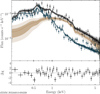Fig. 20

EPIC-pn spectrum of 4XMM J053449.0−694338 with colours as in Fig. 17 visually rebinned for better readability.

7.2.6 A gamma-ray binary embedded in a supernova remnant

While hundreds of interacting binary systems containing a high-mass star and a compact object show emission in X-rays (Liu et al. 2006; Antoniou & Zezas 2016; Haberl & Sturm 2016), very few systems are detectable in gamma-rays. For the creation of gamma-ray emission, non-thermal processes are necessary, such as particle acceleration in the shock of colliding winds of a fast-rotating pulsar and its high-mass companion (Dubus 2006) or high-velocity jets in BH-binaries (Mirabel & Rodríguez 1998). It is expected that HMXBs hosting NSs undergo a short gamma-ray emitting phase shortly after formation, leading to an expected number of approximately 30 such systems in the MW (Meurs & van den Heuvel 1989). Finding fewer gamma-ray binaries might suggest that NSs are born with relatively slow rotation.

CXOU J053600.0−673507 was proposed as an HMXB candidate inside the pulsar wind nebula DEM L241 (Seward et al. 2012; Bamba et al. 2006). Corbet et al. (2016) later identified it as the first extragalactic gamma-ray binary with its gamma-ray counterpart called LMC P3. They consistently find orbital modulation at a period of 10.3 days in radio, X-rays, and gamma-rays.

eROSITA detects CXOU J053600.0−673507 as a point source surrounded by the extended emission of DEM L241. To correctly fit the X-ray spectrum of the HMXB, we need to apply a more sophisticated spectral fit to the background spectrum than the PCA model described in Sect. 4.3. For the off-region, we chose a circle well inside the South head of the supernova remnant (SNR) (see Seward et al. 2012). We then follow Yeung et al. (2023) (Appendix A) to estimate the particle background (PB) contribution in the on- and the off-regions and fit for the sum of PB and the SNR in the off-region and the sum of SNR, PB, and HMXB contributions in the on-region. We account for the positionally non-constant background contribution by the SNR by allowing the normalisations to change between on- and off-regions while tying the spectral shapes. Figure 21 shows the best-fit models and Table 10 gives the best-fit parameters. We detect the source at an average flux of $({4.5}_{- 0.3}^{+ 0.4}) \times 10^{- 13} erg {cm}^{- 2} s^{- 1} (0.2 - 5 keV)$ $Mathematical equation: $\left( {4.5_{ - 0.3}^{ + 0.4}} \right) \times {10^{ - 13}}{\rm{erg}}\,{\rm{c}}{{\rm{m}}^{ - 2}}{{\rm{s}}^{ - 1}}(0.2 - 5{\rm{keV}})$$ , which corresponds to an absorption-corrected luminosity of $({10.9}_{- 1.1}^{+ 1.2}) \times 10^{34} erg s^{- 1}$ $Mathematical equation: $\left( {10.9_{ - 1.1}^{ + 1.2}} \right) \times {10^{34}}{\rm{erg}}\,{{\rm{s}}^{ - 1}}$$ .

7.3 Other BeXRBs

Due to its stable luminosity and long-term behaviour, we conducted XMM-Newton follow-up observations for RX J0516.0−6916 to test its possible membership as a class of persistent BeXRB. Here we present our spectral and timing analysis conducted with eROSITA and XMM-Newton observations. Cowley et al. (1997) first suggested RX J0516.0−6916 as a BeXRB by confirming the optical counterpart of the X-ray source as an early type star, which is claimed to be a Be star. Later works (Negueruela & Coe 2002; Raguzova & Popov 2005) questioned the identification of the optical counterpart as a Be star due to the lack of display of any characteristic Be behaviour. Riquelme et al. (2012) found the source to exhibit Hα emission, which suggests the correct classification as a BeXRB with the Be star switching between periods with and without a decretion disc. During our LCO/FLOYDS observation, the source again shows Hα emission with an equivalent width of (−6.4 ± 0.7) Å at a radial velocity relative to the LMC of (418 ± 83) km s⁻¹, further confirming the Be classification.

Across all eRASSs, we find RX J0516.0−6916 to vary by a factor of ≤10. The merged eROSITA spectrum is best fit by an absorbed power-law with an additional component to account for absorption in the LMC. We find a local absorption of $N_{H, L M C} = ({2.1}_{- 1.7}^{+ 2.2}) \times 10^{21} {cm}^{- 2}$ $Mathematical equation: ${N_{H,LMC}} = \left( {2.1_{ - 1.7}^{ + 2.2}} \right) \times {10^{21}}{\rm{c}}{{\rm{m}}^{ - 2}}$$ , a power-law index of 1.4 ± 0.4 and a flux of $({2.7}_{- 0.4}^{+ 0.5}) \times 10^{- 13} erg {cm}^{- 2} s^{- 1}$ $Mathematical equation: $\left( {2.7_{ - 0.4}^{ + 0.5}} \right) \times {10^{ - 13}}{\rm{erg}}\,{\rm{c}}{{\rm{m}}^{ - 2}}{{\rm{s}}^{ - 1}}$$ for the merged eROSITA spectrum. This corresponds to an absorption-corrected luminosity of $({11.1}_{- 1.1}^{+ 1.7}) \times 10^{34} {ergs}^{- 1}$ $Mathematical equation: $\left( {11.1_{ - 1.1}^{ + 1.7}} \right) \times {10^{34}}{\rm{erg}}{{\rm{s}}^{ - 1}}$$ . The XMM-Newton observations for RX J0516.0−6916 were conducted on 2023-11-13 11:28 – 20:10 (obs.-ID 0923160101). The exposure time after background-flare screening for pn is 13780 s. The spectral and timing analysis was performed similarly to that of 4XMM J053449.0−694338 (see Sect. 7.2.5), with fitting restricted to the range of 0.22 to 7.0 keV for higher S/N and due to the PCA model used for the spectral shape of the background. Our best-fit model is an absorbed power law, without an additional component to account for LMC absorption, with a power-law index of 0.66±0.14. For the flux we find $({9.4}_{- 0.9}^{+ 1.0}) \times 10^{- 14} erg {cm}^{- 2} s^{- 1} (0.2 - 0.7 keV)$ $Mathematical equation: $\left( {9.4_{ - 0.9}^{ + 1.0}} \right) \times {10^{ - 14}}{\rm{erg}}\,{\rm{c}}{{\rm{m}}^{ - 2}}{{\rm{s}}^{ - 1}}(0.2 - 0.7{\rm{keV}})$$ , corresponding to an absorption-corrected luminosity of $({2.87}_{- 0.26}^{+ 0.28}) \times 10^{34} erg s^{- 1}$ $Mathematical equation: $\left( {2.87_{ - 0.26}^{ + 0.28}} \right) \times {10^{34}}{\rm{erg}}\,{{\rm{s}}^{ - 1}}$$ . The EPIC-pn spectrum with the best-fit model is shown in Fig. 22. Correcting the event arrival times to the Solar System barycentre, we created an EPIC-pn light curve and conducted a search for periodic variability using an LS periodogram in the range 10–1000 s. We do not find any significant indication of a period present in the data.

XMMU J050722.1−684758 was discovered as a new BeXRB by Maitra et al. (2021a), probably associated with the SNR MCSNR J0507−6847. The authors confirm the NS nature of the compact object by detecting X-ray pulsations with a periodicity of 570 s and find an absorption-corrected X-ray luminosity of 8.5×10³⁴ erg s⁻¹ (0.2−12 keV).

The merged eROSITA spectrum can best be fit by an absorbed power-law without an additional component to account for local absorption. We find a power-law index of 1.2±0.6 and a flux of $({2.9}_{- 1.0}^{+ 1.6}) \times 10^{- 14} erg {cm}^{- 2} s^{- 1} (0.2 - 5 keV)$ $Mathematical equation: $\left( {2.9_{ - 1.0}^{ + 1.6}} \right) \times {10^{ - 14}}{\rm{erg}}\,{\rm{c}}{{\rm{m}}^{ - 2}}{{\rm{s}}^{ - 1}}(0.2 - 5{\rm{keV}})$$ , corresponding to an absorption-corrected luminosity of $({1.0}_{- 0.3}^{+ 0.4}) \times 10^{34} erg s^{- 1}$ $Mathematical equation: $\left( {1.0_{ - 0.3}^{ + 0.4}} \right) \times {10^{34}}{\rm{erg}}\,{{\rm{s}}^{ - 1}}$$ . The optical counterpart of XMMU J050722.1−684758 was observed with the VLT FLAMES/GIRAFFE spectrograph during six observations between 2008-10-07 and 2009-01-07 (PI: R. E. Mennickent, programme ID 082.D-0575 in the wavelength range 6299−6691 Å (red) at spectral resolutions between 10.2 and 39.1. During our analysis, we found strong double-peaked Hα emission in all six observations, which can be best fit with two Lorentzian line profiles. The red and blue lines lie at radial velocities of approximately +100 km s⁻¹ and −100 km s⁻¹ with respect to the LMC. During the first observation on 2008-10-07, the source was fainter by a factor of ∼5 compared to the other five observations. The variability is consistent with a sinusoidal function with a period of 40.16 d (from OGLE analysis, see Sect. 7.4), excluding the first of the six observations. No such behaviour could be observed for the red line. The results of our spectral analysis can be found in Figs. 23 and 24.

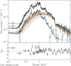Fig. 21

eROSITA spectra of the Gamma-ray binary CXOU J053600.0−673507 merged over all eRASS like Fig. 17. The dark yellow curve shows the best-fit model for the source (absorbed power law). The blue curve and shaded area show the best fit for a sum of particle background and a

vapec

model for the SNR contribution in the on-region. The background spectrum is dominated by the SNR emission up to ∼2 keV, where the particle background takes over. The black curve and shaded area are the sum of the source and background models.

Table 10

Best-fit parameters for CXOU J053600.0−673507.

Fig. 22

Same as Fig. 20 but for RX J0516.0−6916.

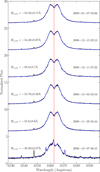Fig. 23

Hα profiles of VLT FLAMES/GIRAFFE observations of the optical counterpart of XMMU J050722.1−684758 between 2008-10-07 and 2009-01-07 shifted to the rest-frame of the LMC. The black line shows the data, the blue line shows the best-fit model using a double-peaked Lorentzian line profile, and the dashed red line indicates the rest-frame wavelength of Hα. Between individual observations, there is a shift of 5.0 in the normalised flux for readability.

7.4 Variability and classification of the optical counterparts

We analysed the OGLE I-band light curves of 28 (candidate) HMXB systems in the LMC in order to find periodicities that are likely related to the binary orbit of the systems. We report eleven new periods (Table D.1), seven from the new candidates discovered in the eROSITA eRASS1 data, supporting their identification as HMXBs. Four periods were identified from previously known systems. From one of them (Swift J0549.7−6812 with period 45.7 d) also the spin period of 6.2 s is known (Krimm et al. 2013b). From the eleven new periods, six are found between 45 d and 170 d, as typical for orbital periods of BeXRBs. Orbital periods of HMXBs shorter than 10 d are usually associated with wind-fed SgXRBs.

Note that this section is self-contained and independent of Sect. 7.2; objects introduced there may also appear here. The analysed OGLE I-band light curves can be found in Fig. D.1 in Kaltenbrunner (2025).

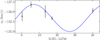Fig. 24

Radial velocity change of the blue component in the double-peaked Hα lines observed from XMMU J050722.1−684758 between 2008-11-28 and 2009-01-07 compared to a sinusoidal fit with a period frozen at the orbital period found with OGLE.

7.4.1 Systems with periods shorter than 10 d

In this section and the following, we discuss our findings for the analysis described in Sect. 4.4. Similar to 1eRASS J054242.7−672752, we find four additional systems with highly significant signals at periods below 10 d. The LS-periodograms around the periods are collected in Fig. 25.

1eRASS J054242.7−672752, used as example in Fig. 5, shows a pair of peaks in the periodograms at 6.49 d and 6.61 d. The periods are consistent with the 1 yr alias (the difference in frequency space is 1 year⁻¹) of each other. We suggest the peak with the highest significance at 6.49 d as the likely orbital period of the system, but cannot rule out the period of 6.61 d.

1eRASS J050705.9−652149 is another such case with the most significant peak at 7.61 d together with the 1 yr alias at 7.77 d. Similarly to the previous case, we propose 7.61 d as the orbital period of the HMXB system, but cannot rule out the period of 7.77 d.

Both 1eRASS J050705.9−652149 and 1eRASS J054242.7− 672752 are candidate Be/WD systems. Likely orbital periods for similar systems are known with 21.5 d (Swift J004427.3− 734801, Haberl et al. 2020c; Coe et al. 2020) and 17.4 d (Swift J011511.0−725611, Kennea et al. 2021b,a) from two Be stars associated with supersoft X-ray sources in the SMC. Orbital periods at the short end of the period distribution seen from BeXRBs suggest tighter orbits for systems with a white dwarf as a compact object with respect to classical BeXRBs with a NS.

The periodograms of 1eRASS J054422.3−672729 are characterised by a highly significant peak at 5.25 d with weaker peaks on both sides, which are consistent with 1 yr aliases. This, together with the relatively bright optical counterpart (V = 13.52 mag) and the X-ray temporal behaviour, identifies this source as an SFXT candidate with a SG in a 5.25 d orbit. While commonly SFXT systems show larger orbital periods than Roche-lobe overflow SgXRBs, there are known SFXT systems with orbital periods of the order of a few days (e.g. Jain et al. 2009).

The highest peaks in the periodograms of RX J0532.5−6551 are found at 3.37 d (P1) and 7.19 d (P2). Smaller peaks around P2 can be related to 1 yr aliases. One-day aliases of P1 and P2 also appear at periods around 1 d. We cannot find a relation between P1 and P2, suggesting two independent periods in the system: 7.19 d, which could be the orbital period, and 1.42 d, which could be the period of NRPs.

4XMM J053449.0−694338 shows a series of four peaks at 1.737 d (P1), 1.879 d (P2), 2.125 d (P3), and 2.341 d (P4), with their corresponding series of 1 d aliases between 0.6 d and 0.7 d. Also, P1 and P4 are 1 d aliases, as well as P2 and P3. P4 could be the alias period of 1 d and 3×P3. It remains unclear if the highest-power peak indicates the fundamental period of 2.125 d, which could be the orbital period of the system, or if it is itself an alias of 0.68 d, suggesting NRPs of a Be star. In addition, the Floyds spectrum showed Hα in absorption (Table 1) and the U−B colour is unusually red (fainter in U than in B), adding a question mark behind the identification of the optical counterpart as O/Be star (Haberl & Sturm 2016). On the other hand, the optical counterpart is too faint (V ∼15 mag) for an SG at LMC distance, and the identification as HMXB needs further confirmation.

7.4.2 Systems with longer periods

Our timing analysis of the OGLE light curves revealed six systems with periods ranging from 45.7 d to 170.3 d. Figure 26 presents the corresponding LS-periodograms, highlighting peaks at these longer periods (Fig. 26).

The I-band light curve of Swift J0549.7−6812 is only sparsely populated with measurements. Nevertheless, a clear peak at 45.7 d is found, with a light curve folded at that period with sinusoidal shape and an amplitude (maximum minus minimum) of ∼0.05 mag. We suggest 45.7 d as the orbital period of an HMXB.

Negueruela & Coe (2002) confirmed RX J0535.0−6700 as a BeXRB in the LMC. Therefore, the period of 241 d reported by Reid et al. (1988) from a UK Schmidt telescope photographic survey was suggested as the likely orbital period of the binary by Haberl & Pietsch (1999b). In our LS periodograms, we detect a relatively sharp peak at 80.5 d, consistent with one-third of the previously reported value, which we cannot confirm in our periodograms. There is also a signal at ∼161 d, which is diffi-cult to filter out of many nearby peaks. Inspection of the light curve between HJD 2458000 and HJD 2459000 reveals a series of strong outbursts, which are 80.5 d apart. However, every other outburst is much stronger than the one before, suggesting that the true underlying period is 161 d. Therefore, we suggest 161 d as the revised orbital period of RX J0535.0−6700. The 241 d period reported earlier might be explained by the much sparser sampling of the UK Schmidt survey compared to OGLE.

The OGLE-IV light curve of 1eRASS J060212.5−674305 is characterised by a slight decrease in brightness over the years. Superimposed are short flares, which increase in their maximum brightness over time. The LS periodograms reveal a peak at ∼122 d, which is also present when removing the flares from the light curve (using only data with I>14.04 mag). Phase folding the light curve data shows that the flares occur at irregular phases. We suggest an orbital period of ∼122 d with the optical flaring activity unrelated to the orbit.

The I-band light curve of 1eRASS J055849.9−675220 shows a scatter of ±0.02 mag without any significant long-term trend. The LS analysis of the light curve without detrending reveals only one significant peak across the full investigated period range at 170 d, which likely indicates the orbital period. The folded light curve is consistent with a sinusoidal profile.

1eRASS J050053.3−653209 shows a somewhat larger scatter of ±0.04 mag on top of small 0.02 mag long-term variations. The most significant peak in the periodograms is found at 160 d, most likely the orbital period. A one-year alias is seen at 285 d. Two additional peaks are found at ∼173 d and ∼180 d. While the latter is probably associated with the 0.5 year period of the window function, 173 d could be an alias of ∼2000 d, related to the length of the light curve. The folded light curve has a triangular profile. However, no significant signal for harmonics are seen in the periodogram.

1eRASS J045028.2−693558 was covered by OGLE-III and OGLE-IV. In addition to a ±0.05 mag scatter, short flares and sharp dips are seen. A highly significant peak is observed in the LS periodograms at 83.89 d. The folded profile is characterised by a broad bump about 0.8 wide in phase and a minimum 0.06 mag fainter than the maximum.

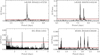Fig. 25

LS periodograms with highly significant peaks at periods below 10 d.

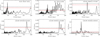Fig. 26

LS periodograms with peaks at longer periods.

7.5 Comparison with SMC population

Compared to the MW, the MCs, particularly the SMC, host a disproportionately large number of HMXBs relative to their stellar mass, likely due to recent episodes of enhanced star formation (Negueruela & Coe 2002; Antoniou et al. 2010; Antoniou & Zezas 2016) and metallicity differences between the galaxies (Linden et al. 2010; Douna et al. 2015). To date the SMC is known to host ∼130 BeXRBs and only one SgXRB (Maravelias et al. 2014; Haberl & Sturm 2016; Vasilopoulos et al. 2017; Kennea et al. 2020; Maitra et al. 2023a). In comparison, in the LMC 59, HMXBs are known, of which 8 are SG systems. The higher abundance of SG systems compared to the SMC can be explained by differences in when recent star formation peaked in the two galaxies (Antoniou et al. 2010; Antoniou & Zezas 2016). The different populations of optical counterparts are also apparent in the V−I over Q plane (see Fig. 8), where counterparts in the LMC display a significantly larger spread than those in the SMC.

Compared to the findings of Sturm et al. (2013) for the SMC, our X-ray luminosity function is less steep at higher luminosities and more closely resembles those reported by Grimm et al. (2003). Additionally, we do not observe a significant change in the power-law index below ∼4×10³⁵ erg s⁻¹, as reported by Sturm et al. (2013). However, this discrepancy may be due to statistical limitations and needs to be confirmed through follow-up observations that probe lower luminosities.

8 Summary

We compiled a comprehensive catalogue of 53 HMXBs in the LMC detected during the first eROSITA all-sky survey (eRASS1), which is complete down to ∼10³⁵ erg s⁻¹. By cross-matching the eRASS1 sources with MCPS, VMC, and a proper-motion selected subsample of the Gaia eDR3 catalogue, we identified and characterised the HMXB population in the LMC.

Out of 60 previously known HMXBs in the LMC, 28 were detected during eRASS1. Additionally, 9 out of 23 previously suggested HMXB candidates were detected, out of which we rejected 5 as HMXBs. We identified 21 new HMXB candidates based on their multi-wavelength properties.

Our analysis utilised the multi-wavelength properties of known HMXBs to define classification flags based on both archival data and follow-up observations, which we used to define six confidence classes. In X-rays, we assessed the spectral properties, the long- and short-term variability, and pulsations. Optical and IR characteristics included Hα emission, IR excess searches from SED fitting, IR colour investigations, and long-term optical variability identification using decades of OGLE data.

The population of HMXBs in the LMC differs notably from that in the SMC, with a higher abundance of systems distinct from the stereotypical Be/NS XRBs, including seven SgXRBs and three (candidate) Be/WD systems. Among the SgXRBs, we identified a new candidate SFXT with phase-dependent flares. Two of the candidate Be/WDs appear in a low-luminosity state, which can be explained by stable accretion on the hotspot of a magnetised WD. These findings highlight the distinct evolutionary pathways and environmental factors influencing HMXB populations in the two Magellanic Clouds.

We constructed the sensitivity-corrected X-ray luminosity function for systems of high confidence classes. A power-law fit to the luminosity function yields an index of ${0.55}_{- 0.11}^{+ 0.53}$ $Mathematical equation: $0.55_{ - 0.11}^{ + 0.53}$$ , in agreement with a previous Chandra-based study that examined the XLFs in several nearby galaxies. Using the X-ray luminosity function, we find that the LMC’s SFR can be estimated with a value of $({0.22}_{- 0.07}^{+ 0.06}) M_{⊙} {yr}^{- 1}$ $Mathematical equation: $\left( {0.22_{ - 0.07}^{ + 0.06}} \right){{\rm{M}}_ \odot }{\rm{y}}{{\rm{r}}^{ - 1}}$$ , which is in agreement with results from other tracers.

Data availability

The full version of our catalogue is available at the CDS via https://cdsarc.cds.unistra.fr/viz-bin/cat/J/A+A/707/A225.

Acknowledgements

We thank the referee for useful comments and suggestions. This work is based on data from eROSITA, the soft X-ray instrument aboard SRG, a joint Russian-German science mission supported by the Russian Space Agency (Roskosmos), in the interests of the Russian Academy of Sciences represented by its Space Research Institute (IKI), and the Deutsches Zentrum für Luft- und Raumfahrt (DLR). The SRG spacecraft was built by Lavochkin Association (NPOL) and its subcontractors, and is operated by NPOL with support from the Max Planck Institute for Extraterrestrial Physics (MPE). The development and construction of the eROSITA X-ray instrument was led by MPE, with contributions from the Dr. Karl Remeis Observatory Bamberg & ECAP (FAU Erlangen-Nürnberg), the University of Hamburg Observatory, the Leibniz Institute for Astrophysics Potsdam (AIP), and the Institute for Astronomy and Astrophysics of the University of Tübingen, with the support of DLR and the Max Planck Society. The Argelander Institute for Astronomy of the University of Bonn and the Ludwig Maximilians Universität Munich also participated in the science preparation for eROSITA. The eROSITA data shown here were processed using the eSASS software system developed by the German eROSITA consortium. This research has made use of the VizieR catalogue access tool, CDS, Strasbourg, France (Ochsenbein 1996). The original description of the VizieR service was published in Ochsenbein et al. (2000). This research has made use of the Spanish Virtual Observatory (https://svo.cab.inta-csic.es) project funded by MCIN/AEI/10.13039/501100011033/ through grant PID2020-112949GB-I00. The LCO observations have been made possible by the support of the Deutsche Forschungsgemeinschaft (DFG, German Research Foundation) under Germany’s Excellence Strategy-EXC-2094-390783311. Based on observations collected at the European Southern Observatory under ESO programme(s) 082.D-0575(A) and/or data obtained from the ESO Science Archive Facility with DOI(s) under https://doi.org/10.18727/archive/27. R.W. is funded by the Deutsche Forschungsgemeinschaft (DFG, German Research Foundation) – 446281683. G.V. acknowledges support from the Hellenic Foundation for Research and Innovation (H.F.R.I.) through the project ASTRAPE (Project ID 7802). A.U. acknowledges support from the “Copernicus 2024 Award” of the Polish FNP and German DFG agencies.

References

Aidelman, Y., & Cidale, L. S. 2023, Galaxies, 11, 31 [NASA ADS] [CrossRef] [Google Scholar]
Antoniou, V., & Zezas, A. 2016, MNRAS, 459, 528 [Google Scholar]
Antoniou, V., Zezas, A., Hatzidimitriou, D., & Kalogera, V. 2010, ApJ, 716, L140 [NASA ADS] [CrossRef] [Google Scholar]
Arnaud, K. A. 1996, ASP Conf. Ser., 101, 17 [Google Scholar]
Assef, R. J., Stern, D., Noirot, G., et al. 2018, ApJS, 234, 23 [Google Scholar]
Astropy Collaboration (Robitaille, T. P., et al.) 2013, A&A, 558, A33 [NASA ADS] [CrossRef] [EDP Sciences] [Google Scholar]
Astropy Collaboration (Price-Whelan, A. M., et al.) 2018, AJ, 156, 123 [Google Scholar]
Astropy Collaboration (Price-Whelan, A. M., et al.) 2022, ApJ, 935, 167 [NASA ADS] [CrossRef] [Google Scholar]
Bailer-Jones, C. A. L., Fouesneau, M., & Andrae, R. 2019, VizieR Online Data Catalog: Gaia DR2 quasar and galaxy classification (Bailer-Jones+, 2019), VizieR On-line Data Catalog: VII/285 [Google Scholar]
Balona, L. A. 2000, ASP Conf. Ser., 214, 1 [Google Scholar]
Bamba, A., Ueno, M., Nakajima, H., Mori, K., & Koyama, K. 2006, A&A, 450, 585 [NASA ADS] [CrossRef] [EDP Sciences] [Google Scholar]
Bodensteiner, J., Sana, H., Dufton, P. L., et al. 2023, A&A, 680, A32 [NASA ADS] [CrossRef] [EDP Sciences] [Google Scholar]
Bonanos, A. Z., Lennon, D. J., Köhlinger, F., et al. 2010, AJ, 140, 416 [NASA ADS] [CrossRef] [Google Scholar]
Bozzo, E., Falanga, M., & Stella, L. 2008, ApJ, 683, 1031 [Google Scholar]
Brown, T. M., Baliber, N., Bianco, F. B., et al. 2013, PASP, 125, 1031 [Google Scholar]
Brunner, H., Liu, T., Lamer, G., et al. 2022, A&A, 661, A1 [NASA ADS] [CrossRef] [EDP Sciences] [Google Scholar]
Buchner, J. 2021a, J. Open Source Softw., 6, 3045 [NASA ADS] [CrossRef] [Google Scholar]
Buchner, J. 2021b, J. Open Source Softw., 6, 3001 [CrossRef] [Google Scholar]
Charles, P. A., Booth, L., Densham, R. H., et al. 1983, MNRAS, 202, 657 [NASA ADS] [Google Scholar]
Charles, P. A., Rajoelimanana, A., & Maccarone, T. J. 2011, ATel., 3751, 1 [Google Scholar]
Cioni, M. R. L., et al. 2023, VizieR Online Data Catalog: VISTA Magellanic Survey (VMC) catalog (YJKs) DR6 (Cioni+, 2011), VizieR On-line Data Catalog: II/375 [Google Scholar]
Cioni, M. R. L., Clementini, G., Girardi, L., et al. 2011, A&A, 527, A116 [CrossRef] [EDP Sciences] [Google Scholar]
Cioni, M. R. L., Kamath, D., Rubele, S., et al. 2013, A&A, 549, A29 [NASA ADS] [CrossRef] [EDP Sciences] [Google Scholar]
Coe, M. J., Negueruela, I., Buckley, D. A. H., Haigh, N. J., & Laycock, S. G. T. 2001, MNRAS, 324, 6234 [Google Scholar]
Coe, M. J., Finger, M., Bartlett, E. S., & Udalski, A. 2015, MNRAS, 447, 1630 [Google Scholar]
Coe, M. J., Kennea, J. A., Evans, P. A., & Udalski, A. 2020, MNRAS, 497, L50 [NASA ADS] [CrossRef] [Google Scholar]
Coe, M. J., Kennea, J. A., Monageng, I. M., et al. 2023, MNRAS, 524, 3263 [Google Scholar]
Corbet, R. H. D., Chomiuk, L., Coe, M. J., et al. 2016, ApJ, 829, 105 [Google Scholar]
Cowley, A. P., Crampton, D., Hutchings, J. B., Remillard, R., & Penfold, J. E. 1983, ApJ, 272, 118 [Google Scholar]
Cowley, A. P., Schmidtke, P. C., McGrath, T. K., et al. 1997, PASP, 109, 21 [NASA ADS] [CrossRef] [Google Scholar]
Crawford, D. F., Jauncey, D. L., & Murdoch, H. S. 1970, ApJ, 162, 405 [Google Scholar]
Crawford, S. M., Still, M., Schellart, P., et al. 2010, SPIE Conf. Ser., 7737, 773725 [Google Scholar]
de Wit, W. J., Lamers, H. J. G. L. M., Marquette, J. B., & Beaulieu, J. P. 2006, A&A, 456, 1027 [NASA ADS] [CrossRef] [EDP Sciences] [Google Scholar]
Dickey, J. M., & Lockman, F. J. 1990, ARA&A, 28, 215 [NASA ADS] [CrossRef] [Google Scholar]
Douna, V. M., Pellizza, L. J., Mirabel, I. F., & Pedrosa, S. E. 2015, A&A, 579, A44 [NASA ADS] [CrossRef] [EDP Sciences] [Google Scholar]
Dubus, G. 2006, A&A, 456, 801 [NASA ADS] [CrossRef] [EDP Sciences] [Google Scholar]
Ducci, L., Mereghetti, S., Santangelo, A., et al. 2022, A&A, 661, A22 [NASA ADS] [CrossRef] [EDP Sciences] [Google Scholar]
Esin, A. A., McClintock, J. E., & Narayan, R. 1997, ApJ, 489, 865 [NASA ADS] [CrossRef] [Google Scholar]
Evans, C. J., Taylor, W. D., Hénault-Brunet, V., et al. 2011, A&A, 530, A108 [NASA ADS] [CrossRef] [EDP Sciences] [Google Scholar]
Falanga, M., Bozzo, E., Lutovinov, A., et al. 2015, A&A, 577, A130 [NASA ADS] [CrossRef] [EDP Sciences] [Google Scholar]
Ferrigno, C., Bozzo, E., & Romano, P. 2022, A&A, 664, A99 [NASA ADS] [CrossRef] [EDP Sciences] [Google Scholar]
Flesch, E. W. 2023, VizieR Online Data Catalog: The Million Quasars (Milliquas) catalogue, version 8 (Flesch, 2023), VizieR On-line Data Catalog: VII/294 [Google Scholar]
Gaia Collaboration (Luri, X., et al.) 2021, A&A, 649, A7 [EDP Sciences] [Google Scholar]
Gamen, R., Barbà, R. H., Walborn, N. R., et al. 2015, A&A, 583, L4 [NASA ADS] [CrossRef] [EDP Sciences] [Google Scholar]
Goossens, M. E., Bird, A. J., Drave, S. P., et al. 2013, MNRAS, 434, 2182 [NASA ADS] [CrossRef] [Google Scholar]
Gordon, K. D., Clayton, G. C., Decleir, M., et al. 2023, ApJ, 950, 86 [CrossRef] [Google Scholar]
Greiner, J., Bornemann, W., Clemens, C., et al. 2008, PASP, 120, 405 [Google Scholar]
Grimm, H.-J., Gilfanov, M., & Sunyaev, R. 2003, Chinese J. Astron. Astrophys. Suppl., 3, 257 [Google Scholar]
Grundstrom, E. D., & Gies, D. R. 2006, ApJ, 651, L53 [NASA ADS] [CrossRef] [Google Scholar]
Haberl, F., & Pietsch, W. 1999a, A&AS, 139, 277 [Google Scholar]
Haberl, F., & Pietsch, W. 1999b, A&A, 344, 521 [NASA ADS] [Google Scholar]
Haberl, F., & Sturm, R. 2016, A&A, 586, A81 [NASA ADS] [CrossRef] [EDP Sciences] [Google Scholar]
Haberl, F., Pietsch, W., & Dennerl, K. 1995, A&A, 303, L49 [NASA ADS] [Google Scholar]
Haberl, F., Dennerl, K., Pietsch, W., & Reinsch, K. 1997, A&A, 318, 490 [Google Scholar]
Haberl, F., Dennerl, K., & Pietsch, W. 2003, A&A, 406, 471 [NASA ADS] [CrossRef] [EDP Sciences] [Google Scholar]
Haberl, F., Israel, G. L., Rodriguez Castillo, G. A., et al. 2017, A&A, 598, A69 [NASA ADS] [CrossRef] [EDP Sciences] [Google Scholar]
Haberl, F., Maitra, C., Carpano, S., et al. 2020a, ATel, 13609, 1 [Google Scholar]
Haberl, F., Maitra, C., Greiner, J., et al. 2020b, ATel, 13789, 1 [Google Scholar]
Haberl, F., Maitra, C., Greiner, J., et al. 2020c, ATel, 13709, 1 [Google Scholar]
Haberl, F., Wilms, J., Gokus, A., et al. 2020d, ATel, 13828, 1 [NASA ADS] [Google Scholar]
Haberl, F., Salganik, A., Maitra, C., et al. 2021, ATel, 15133, 1 [NASA ADS] [Google Scholar]
Haberl, F., Maitra, C., Vasilopoulos, G., et al. 2022, A&A, 662, A22 [NASA ADS] [CrossRef] [EDP Sciences] [Google Scholar]
Haberl, F., Maitra, C., Kaltenbrunner, D., et al. 2023, A&A, 671, A90 [NASA ADS] [CrossRef] [EDP Sciences] [Google Scholar]
Haberl, F., Xu, Y., Maitra, C., et al. 2025, MNRAS, 542, 583 [Google Scholar]
Hanuschik, R. W., Kozok, J. R., & Kaiser, D. 1988, A&A, 189, 147 [NASA ADS] [Google Scholar]
Harris, J., & Zaritsky, D. 2004, AJ, 127, 1531 [NASA ADS] [CrossRef] [Google Scholar]
Harris, J., & Zaritsky, D. 2009, AJ, 138, 1243 [NASA ADS] [CrossRef] [Google Scholar]
Hippke, M., David, T. J., Mulders, G. D., & Heller, R. 2019, AJ, 158, 143 [Google Scholar]
Hog, E., Fabricius, C., Makarov, V. V., et al. 2000, VizieR Online Data Catalog: The Tycho-2 Catalogue (Hog+ 2000), VizieR On-line Data Catalog: I/259 [Google Scholar]
Howarth, I. D. 2013, A&A, 555, A141 [NASA ADS] [CrossRef] [EDP Sciences] [Google Scholar]
Hutchings, J. B., Crampton, D., & Cowley, A. P. 1983, ApJ, 275, L43 [NASA ADS] [CrossRef] [Google Scholar]
Inam, S. Ç., Townsend, L. J., McBride, V. A., et al. 2009, MNRAS, 395, 1662 [Google Scholar]
in’t Zand, J. J. M. 2005, A&A, 441, L1 [CrossRef] [EDP Sciences] [Google Scholar]
Jain, C., Paul, B., & Dutta, A. 2009, MNRAS, 397, L11 [NASA ADS] [CrossRef] [Google Scholar]
Jansen, F., Lumb, D., Altieri, B., et al. 2001, A&A, 365, L1 [NASA ADS] [CrossRef] [EDP Sciences] [Google Scholar]
Jaxon, E. G., Guerrero, M. A., Howk, J. C., et al. 2001, PASP, 113, 1130 [Google Scholar]
Joss, P. C., & Rappaport, S. A. 1984, ARA&A, 22, 537 [Google Scholar]
Kahabka, P., de Boer, K. S., & Brüns, C. 2001, A&A, 371, 816 [NASA ADS] [CrossRef] [EDP Sciences] [Google Scholar]
Kahabka, P., Haberl, F., Payne, J. L., & Filipović, M. D. 2006, A&A, 458, 285 [NASA ADS] [CrossRef] [EDP Sciences] [Google Scholar]
Kaltenbrunner, D. 2025, A comprehensive catalogue of High-Mass Xray binaries in the Large Magellanic Cloud detected during the first eROSITA all-sky survey - Appendix Figures and Tables, available at DOI: 10.5281/zenodo.17833631 [Google Scholar]
Kaufer, A., Stahl, O., Tubbesing, S., et al. 1999, The Messenger, 95, 8 [Google Scholar]
Kennea, J. A., Coe, M. J., Evans, P. A., et al. 2020, ATel, 13823, 1 [Google Scholar]
Kennea, J. A., Coe, M. J., Evans, P. A., et al. 2021a, MNRAS, 508, 781 [NASA ADS] [CrossRef] [Google Scholar]
Kennea, J. A., Coe, M. J., Evans, P. A., et al. 2021b, ATel, 14341, 1 [Google Scholar]
Kim, D.-W., Protopapas, P., Trichas, M., et al. 2012, ApJ, 747, 107 [NASA ADS] [CrossRef] [Google Scholar]
Kovlakas, K., Zezas, A., Andrews, J. J., et al. 2021, MNRAS, 506, 1896 [NASA ADS] [CrossRef] [Google Scholar]
Kozłowski, S., & Kochanek, C. S. 2009, ApJ, 701, 508 [CrossRef] [Google Scholar]
Kozłowski, S., Onken, C. A., Kochanek, C. S., et al. 2013, ApJ, 775, 92 [CrossRef] [Google Scholar]
Krimm, H. A., Corbet, R. H. D., Evans, P. A., et al. 2009, ATel, 2011, 1 [Google Scholar]
Krimm, H. A., Barthelmy, S. D., Baumgartner, W., et al. 2013a, ATel, 5286, 1 [Google Scholar]
Krimm, H. A., Gelbord, J. M., Holland, S. T., & Kennea, J. A. 2013b, ATel, 5309, 1 [Google Scholar]
Krimm, H. A., Holland, S. T., & Kennea, J. A. 2013c, ATel, 5293, 1 [Google Scholar]
La Palombara, N., & Mereghetti, S. 2007, A&A, 474, 137 [NASA ADS] [CrossRef] [EDP Sciences] [Google Scholar]
La Palombara, N., Sidoli, L., Esposito, P., Tiengo, A., & Mereghetti, S. 2009, A&A, 505, 947 [NASA ADS] [CrossRef] [EDP Sciences] [Google Scholar]
La Palombara, N., Sidoli, L., Esposito, P., Tiengo, A., & Mereghetti, S. 2012, A&A, 539, A82 [NASA ADS] [CrossRef] [EDP Sciences] [Google Scholar]
Lanz, T., & Hubeny, I. 2003, ApJS, 146, 417 [NASA ADS] [CrossRef] [Google Scholar]
Lanz, T., & Hubeny, I. 2007, ApJS, 169, 83 [CrossRef] [Google Scholar]
Linden, T., Kalogera, V., Sepinsky, J. F., et al. 2010, ApJ, 725, 1984 [Google Scholar]
Liu, Q. Z., van Paradijs, J., & van den Heuvel, E. P. J. 2005, A&A, 442, 1135 [NASA ADS] [CrossRef] [EDP Sciences] [Google Scholar]
Liu, Q. Z., van Paradijs, J., & van den Heuvel, E. P. J. 2006, A&A, 455, 1165 [NASA ADS] [CrossRef] [EDP Sciences] [Google Scholar]
Lomb, N. R. 1976, Ap&SS, 39, 447 [Google Scholar]
Luck, R. E., Moffett, T. J., Barnes, T. G., III, & Gieren, W. P. 1998, AJ, 115, 605 [NASA ADS] [CrossRef] [Google Scholar]
Maggi, P., Haberl, F., Sturm, R., et al. 2013, A&A, 554, A1 [NASA ADS] [CrossRef] [EDP Sciences] [Google Scholar]
Maggi, P., Haberl, F., Kavanagh, P. J., et al. 2016, A&A, 585, A162 [NASA ADS] [CrossRef] [EDP Sciences] [Google Scholar]
Maitra, C., & Haberl, F. 2022, A&A, 657, A26 [NASA ADS] [CrossRef] [EDP Sciences] [Google Scholar]
Maitra, C., Haberl, F., Filipović, M. D., et al. 2019a, MNRAS, 490, 5494 [Google Scholar]
Maitra, C., Haberl, F., Ivanov, V. D., Cioni, M.-R. L., & van Loon, J. T. 2019b, A&A, 622, A29 [NASA ADS] [CrossRef] [EDP Sciences] [Google Scholar]
Maitra, C., Haberl, F., Carpano, S., et al. 2020a, ATel, 13610, 1 [Google Scholar]
Maitra, C., Haberl, F., Koenig, O., et al. 2020b, ATel, 13650, 1 [NASA ADS] [Google Scholar]
Maitra, C., Haberl, F., Maggi, P., et al. 2021a, MNRAS, 504, 326 [NASA ADS] [CrossRef] [Google Scholar]
Maitra, C., Haberl, F., Vasilopoulos, G., et al. 2021b, A&A, 647, A8 [NASA ADS] [CrossRef] [EDP Sciences] [Google Scholar]
Maitra, C., Haberl, F., Kaltenbrunner, D., et al. 2023a, ATel, 15886, 1 [NASA ADS] [Google Scholar]
Maitra, C., Kaltenbrunner, D., Haberl, F., et al. 2023b, A&A, 669, A30 [NASA ADS] [CrossRef] [EDP Sciences] [Google Scholar]
Maravelias, G., Zezas, A., Antoniou, V., & Hatzidimitriou, D. 2014, MNRAS, 438, 2005 [NASA ADS] [CrossRef] [Google Scholar]
Marino, A., Yang, H. N., Coti Zelati, F., et al. 2025, ApJ, 980, L36 [Google Scholar]
Mark, H., Price, R., Rodrigues, R., Seward, F. D., & Swift, C. D. 1969, ApJ, 155, L143 [NASA ADS] [CrossRef] [Google Scholar]
Martínez-Núñez, S., Kretschmar, P., Bozzo, E., et al. 2017, Space Sci. Rev., 212, 59 [Google Scholar]
Mateos, S., Alonso-Herrero, A., Carrera, F. J., et al. 2012, MNRAS, 426, 3271 [Google Scholar]
Mennickent, R. E., Pietrzyński, G., Gieren, W., & Szewczyk, O. 2002, A&A, 393, 887 [NASA ADS] [CrossRef] [EDP Sciences] [Google Scholar]
Merloni, A., Lamer, G., Liu, T., et al. 2024, A&A, 682, A34 [NASA ADS] [CrossRef] [EDP Sciences] [Google Scholar]
Meurs, E. J. A., & van den Heuvel, E. P. J. 1989, A&A, 226, 88 [NASA ADS] [Google Scholar]
Mirabel, I. F., & Rodríguez, L. F. 1998, Nature, 392, 673 [NASA ADS] [CrossRef] [Google Scholar]
Negueruela, I., & Coe, M. J. 2002, A&A, 385, 517 [NASA ADS] [CrossRef] [EDP Sciences] [Google Scholar]
Ochsenbein, F. 1996, The VizieR database of astronomical catalogues [Google Scholar]
Ochsenbein, F., Bauer, P., & Marcout, J. 2000, A&AS, 143, 23 [Google Scholar]
Orosz, J. A., Steeghs, D., McClintock, J. E., et al. 2009, ApJ, 697, 573 [NASA ADS] [CrossRef] [Google Scholar]
Orosz, J. A., Steiner, J. F., McClintock, J. E., et al. 2014, ApJ, 794, 154 [NASA ADS] [CrossRef] [Google Scholar]
Pasquini, L., Avila, G., Blecha, A., et al. 2002, The Messenger, 110, 1 [Google Scholar]
Pennock, C. M., van Loon, J. T., Filipovic, M. D., et al. 2021, VizieR Online Data Catalog: ASKAP-EMU ESP LMC Radio Continuum Survey (Pennock+, 2021), VizieR On-line Data Catalog: J/MNRAS/506/3540 [Google Scholar]
Pfahl, E., Rappaport, S., Podsiadlowski, P., & Spruit, H. 2002, ApJ, 574, 364 [Google Scholar]
Pietrzyński, G., Graczyk, D., Gallenne, A., et al. 2019, Nature, 567, 200 [Google Scholar]
Pols, O. R., Cote, J., Waters, L. B. F. M., & Heise, J. 1991, A&A, 241, 419 [NASA ADS] [Google Scholar]
Porter, J. M., & Rivinius, T. 2003, PASP, 115, 1153 [Google Scholar]
Predehl, P., Andritschke, R., Arefiev, V., et al. 2021, A&A, 647, A1 [EDP Sciences] [Google Scholar]
Raguzova, N. V. 2001, A&A, 367, 848 [NASA ADS] [CrossRef] [EDP Sciences] [Google Scholar]
Raguzova, N. V., & Popov, S. B. 2005, Astron. Astrophys. Trans., 24, 151 [Google Scholar]
Reid, N., Glass, I. S., & Catchpole, R. M. 1988, MNRAS, 232, 53 [Google Scholar]
Reig, P., & Nespoli, E. 2013, A&A, 551, A1 [NASA ADS] [CrossRef] [EDP Sciences] [Google Scholar]
Reig, P., & Roche, P. 1999, MNRAS, 306, 100 [NASA ADS] [CrossRef] [Google Scholar]
Remillard, R. A., & McClintock, J. E. 2006, ARA&A, 44, 49 [Google Scholar]
Richter, O. G., Tammann, G. A., & Huchtmeier, W. K. 1987, A&A, 171, 33 [Google Scholar]
Riquelme, M. S., Torrejón, J. M., & Negueruela, I. 2012, A&A, 539, A114 [NASA ADS] [CrossRef] [EDP Sciences] [Google Scholar]
Rivinius, T., Baade, D., & Štefl, S. 2003, A&A, 411, 229 [NASA ADS] [CrossRef] [EDP Sciences] [Google Scholar]
Rodrigo, C., & Solano, E. 2020, in XIV.0 Scientific Meeting (virtual) of the Spanish Astronomical Society, 182 [Google Scholar]
Rodrigo, C., Solano, E., & Bayo, A. 2012, SVO Filter Profile Service Version 1.0, IVOA Working Draft 15 October 2012 [Google Scholar]
Rolleston, W. R. J., Trundle, C., & Dufton, P. L. 2002, A&A, 396, 53 [NASA ADS] [CrossRef] [EDP Sciences] [Google Scholar]
Romano, P. 2015, J. High Energy Astrophys., 7, 126 [Google Scholar]
Sabogal, B. E., Mennickent, R. E., Pietrzyński, G., & Gieren, W. 2005, MNRAS, 361, 1055 [NASA ADS] [CrossRef] [Google Scholar]
Salganik, A., Tsygankov, S. S., Lutovinov, A. A., et al. 2022, MNRAS, 514, 4018 [NASA ADS] [CrossRef] [Google Scholar]
Sasaki, M., Haberl, F., & Pietsch, W. 2000, A&AS, 143, 391 [Google Scholar]
Savitzky, A., & Golay, M. J. E. 1964, Anal. Chem., 36, 1627 [Google Scholar]
Saxton, R. D., König, O., Descalzo, M., et al. 2022, Astron. Comput., 38, 100531 [NASA ADS] [CrossRef] [Google Scholar]
Scargle, J. D. 1982, ApJ, 263, 835 [Google Scholar]
Scargle, J. D. 1998, ApJ, 504, 405 [Google Scholar]
Scargle, J. D., Norris, J. P., Jackson, B., & Chiang, J. 2013a, ApJ, 764, 167 [Google Scholar]
Scargle, J. D., Norris, J. P., Jackson, B., & Chiang, J. 2013b, arXiv e-prints [arXiv:1304.2818] [Google Scholar]
Schmidtke, P. C., Cowley, A. P., Frattare, L. M., et al. 1994, PASP, 106, 843 [NASA ADS] [CrossRef] [Google Scholar]
Schmidtke, P. C., Cowley, A. P., Hauschildt, P. H., et al. 1996, PASP, 108, 668 [Google Scholar]
Secrest, N. J., Dudik, R. P., Dorland, B. N., et al. 2015, ApJS, 221, 12 [NASA ADS] [CrossRef] [Google Scholar]
Sen, K., Xu, X. T., Langer, N., et al. 2021, A&A, 652, A138 [NASA ADS] [CrossRef] [EDP Sciences] [Google Scholar]
Sen, K., El Mellah, I., Langer, N., et al. 2024, A&A, 690, A256 [NASA ADS] [CrossRef] [EDP Sciences] [Google Scholar]
Seward, F. D., Charles, P. A., Foster, D. L., et al. 2012, ApJ, 759, 123 [Google Scholar]
Shakura, N. I., & Sunyaev, R. A. 1973, A&A, 24, 337 [NASA ADS] [Google Scholar]
Shakura, N., Postnov, K., Kochetkova, A., & Hjalmarsdotter, L. 2012, MNRAS, 420, 216 [Google Scholar]
Shtykovskiy, P., & Gilfanov, M. 2005a, A&A, 431, 597 [NASA ADS] [CrossRef] [EDP Sciences] [Google Scholar]
Shtykovskiy, P., & Gilfanov, M. 2005b, MNRAS, 362, 879 [NASA ADS] [CrossRef] [Google Scholar]
Sidoli, L., Paizis, A., & Mereghetti, S. 2006, A&A, 450, L9 [NASA ADS] [CrossRef] [EDP Sciences] [Google Scholar]
Sidoli, L., Ponti, G., Sguera, V., & Esposito, P. 2023, A&A, 671, A150 [NASA ADS] [CrossRef] [EDP Sciences] [Google Scholar]
Skibba, R. A., Engelbracht, C. W., Aniano, G., et al. 2012, ApJ, 761, 42 [NASA ADS] [CrossRef] [Google Scholar]
Skowron, D. M., Skowron, J., Udalski, A., et al. 2021, ApJS, 252, 23 [Google Scholar]
Slettebak, A. 1988, PASP, 100, 770 [NASA ADS] [CrossRef] [Google Scholar]
Smith, D. M., Markwardt, C. B., Swank, J. H., & Negueruela, I. 2012, MNRAS, 422, 2661 [NASA ADS] [CrossRef] [Google Scholar]
Soria, R., Wu, K., Page, M. J., & Sakelliou, I. 2001, A&A, 365, L273 [NASA ADS] [CrossRef] [EDP Sciences] [Google Scholar]
Souchay, J., Gattano, C., Andrei, A. H., et al. 2019, VizieR Online Data Catalog: Astrometric Catalogue 5, LQAC-5 (Souchay+, 2019), VizieR On-line Data Catalog: J/A+A/624/A145 [Google Scholar]
Stan Development Team 2024, Stan Modeling Language Users Guide and Reference Manual v2.34, https://mc-stan.org/docs/reference-manual/ [Google Scholar]
Straizys, V., Lazauskaite, R., Liubertas, R., & Azusienis, A. 1998, Balt. Astron., 7, 605 [Google Scholar]
Strüder, L., Briel, U., Dennerl, K., et al. 2001, A&A, 365, L18 [Google Scholar]
Sturm, R., Haberl, F., & Pietsch, W. 2011a, ATel, 3747, 1 [Google Scholar]
Sturm, R., Haberl, F., & Pietsch, W. 2011b, ATel, 3753, 1 [Google Scholar]
Sturm, R., Haberl, F., Pietsch, W., et al. 2012a, A&A, 537, A76 [NASA ADS] [CrossRef] [EDP Sciences] [Google Scholar]
Sturm, R., Haberl, F., Pietsch, W., Immler, S., & Udalski, A. 2012b, ATel, 3993, 1 [Google Scholar]
Sturm, R., Haberl, F., Pietsch, W., et al. 2013, A&A, 558, A3 [NASA ADS] [CrossRef] [EDP Sciences] [Google Scholar]
Sun, N.-C., de Grijs, R., Subramanian, S., et al. 2017, ApJ, 849, 149 [Google Scholar]
Sunyaev, R., Arefiev, V., Babyshkin, V., et al. 2021, A&A, 656, A132 [NASA ADS] [CrossRef] [EDP Sciences] [Google Scholar]
Treiber, H., Vasilopoulos, G., Bailyn, C. D., et al. 2021, MNRAS, 503, 6187 [CrossRef] [Google Scholar]
Treiber, H., Vasilopoulos, G., Bailyn, C. D., Haberl, F., & Udalski, A. 2025, A&A, 694, A43 [NASA ADS] [CrossRef] [EDP Sciences] [Google Scholar]
Turner, M. J. L., Abbey, A., Arnaud, M., et al. 2001, A&A, 365, L27 [CrossRef] [EDP Sciences] [Google Scholar]
Udalski, A. 2008, Acta Astron., 58, 187 [NASA ADS] [Google Scholar]
Udalski, A., Szymanski, M., Kaluzny, J., Kubiak, M., & Mateo, M. 1992, Acta Astron., 42, 253 [NASA ADS] [Google Scholar]
Udalski, A., Szymanski, M. K., Soszynski, I., & Poleski, R. 2008, Acta Astron., 58, 69 [NASA ADS] [Google Scholar]
Udalski, A., Szymański, M. K., & Szymański, G. 2015, Acta Astron., 65, 1 [NASA ADS] [Google Scholar]
Valenti, S., Dand, D., & Howell, D. A. 2013, FLOYDS Manual and Pipeline, https://www.authorea.com/users/598/articles/6566 [Google Scholar]
van Jaarsveld, N., Buckley, D. A. H., McBride, V. A., et al. 2018, MNRAS, 475, 3253 [Google Scholar]
Vasilopoulos, G. 2025, A&A, 698, A26 [NASA ADS] [CrossRef] [EDP Sciences] [Google Scholar]
Vasilopoulos, G., Maggi, P., Haberl, F., et al. 2013a, A&A, 558, A74 [NASA ADS] [CrossRef] [EDP Sciences] [Google Scholar]
Vasilopoulos, G., Sturm, R., Haberl, F., Maggi, P., & Udalski, A. 2013b, ATel, 5540, 1 [Google Scholar]
Vasilopoulos, G., Haberl, F., Sturm, R., Maggi, P., & Udalski, A. 2014, A&A, 567, A129 [NASA ADS] [CrossRef] [EDP Sciences] [Google Scholar]
Vasilopoulos, G., Zezas, A., Antoniou, V., & Haberl, F. 2017, MNRAS, 470, 4354 [NASA ADS] [CrossRef] [Google Scholar]
Vasilopoulos, G., Maitra, C., Haberl, F., Hatzidimitriou, D., & Petropoulou, M. 2018, MNRAS, 475, 220 [Google Scholar]
Vasilopoulos, G., Ray, P. S., Gendreau, K. C., et al. 2020, MNRAS, 494, 5350 [NASA ADS] [CrossRef] [Google Scholar]
Walter, R., Lutovinov, A. A., Bozzo, E., & Tsygankov, S. S. 2015, A&A Rev., 23, 2 [Google Scholar]
White, N. E., & Marshall, F. E. 1984, ApJ, 281, 354 [Google Scholar]
Willingale, R., Starling, R. L. C., Beardmore, A. P., Tanvir, N. R., & O’Brien, P. T. 2013, MNRAS, 431, 394 [Google Scholar]
Wilms, J., Allen, A., & McCray, R. 2000, ApJ, 542, 914 [Google Scholar]
Yang, H. N., Maitra, C., Vasilopoulos, G., et al. 2025, MNRAS, 536, 1357 [Google Scholar]
Yeung, M. C. H., Freyberg, M. J., Ponti, G., et al. 2023, A&A, 676, A3 [NASA ADS] [CrossRef] [EDP Sciences] [Google Scholar]
Zaritsky, D., Harris, J., Thompson, I. B., Grebel, E. K., & Massey, P. 2002, AJ, 123, 855 [Google Scholar]
Zaritsky, D., Harris, J., Thompson, I. B., & Grebel, E. K. 2004, AJ, 128, 1606 [Google Scholar]

https://vizier.cds.unistra.fr/

https://archive.eso.org/scienceportal/home

http://xmmuls.esac.esa.int/upperlimitserver/

⁴

https://lco.global/documentation/data/floyds-pipeline/

⁵

https://iraf-community.github.io/

⁶

https://simbad.cds.unistra.fr/simbad/

⁷

https://mc-stan.org/cmdstanpy/

⁸

https://docs.astropy.org/en/stable/timeseries/lombscargle.html

⁹

https://www.cosmos.esa.int/web/xmm-newton/sas-release-notes-2210/

Appendix A Supplementary X-ray material

Table A.1

Alternative names and literature references for discovery of the X-ray sources with confidence class 1 in our HMXB catalogue.

References: See Table A.2.

Table A.2

Same as Table A.1 for confidence classes 2−6.

References: HMV22: Haberl et al. (2022), VSH13: Vasilopoulos et al. (2013b), SCF94: Schmidtke et al. (1994), SCH96: Schmidtke et al. (1996), MHM21: Maitra et al. (2021a), MHS13: Maggi et al. (2013), HMC20: Haberl et al. (2020a), HIR17: Haberl et al. (2017), KCE09: Krimm et al. (2009), CFB15: Coe et al. (2015), CSM97: Cowley et al. (1997), KdBB01: Kahabka et al. (2001), CNB01: Coe et al. (2001), HP99: Haberl & Pietsch (1999a), vJBM18: van Jaarsveld et al. (2018), MHC20: Maitra et al. (2020a), MHK20: Maitra et al. (2020b), HDP97: Haberl et al. (1997), HDP03: Haberl et al. (2003), VMH13: Vasilopoulos et al. (2013a), VMH18: Vasilopoulos et al. (2018), HPD95: Haberl et al. (1995), JR84: Joss & Rappaport (1984), NC02: Negueruela & Coe (2002), CBD83: Charles et al. (1983), BUN06: Bamba et al. (2006), CCC16: Corbet et al. (2016), CCH83: Cowley et al. (1983), HCC83: Hutchings et al. (1983), WM84: White & Marshall (1984), SG05: Shtykovskiy & Gilfanov (2005a), ITM09: Inam et al. (2009), KBB13: Krimm et al. (2013a), KGH13: Krimm et al. (2013b), HMG20: Haberl et al. (2020b), SHP12: Sturm et al. (2012b), SHP00: Sasaki et al. (2000).

The merged eROSITA spectra, eROSITA light curves and long-term light curves for all systems investigated in this work can be found in Kaltenbrunner (2025) Fig. A.1, Fig. A.2 and Fig. A.3, respectively. Examples can be found in Fig. A.1, Fig. A.2 and Fig. A.3. For all sources, Tables A.3 and A.4 in Kaltenbrunner (2025) list the effective eRASS:5 exposure times and luminosities derived from fits to the merged eRASS:5 spectra. Note that the effective exposures of LMC X−1 (#25), LMC X−3 (#24), and LMC X−4 (#20) are significantly lower because their extraction regions were restricted to mitigate photon pile-up (see Sect. 4.1).

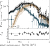Fig. A.1

Example for Fig. A.1 in Kaltenbrunner (2025). Merged eROSITA spectrum with best fit models for #1. Black and blue data points are fluxes in the on- and off-region, respectively. Blue and yellow lines show the best-fit models for the background and source, the black line shows the sum of both. Shaded areas display the 1σ (dark) and 3σ (light) confidence for the models.

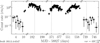Fig. A.2

Example for Fig. A.2 in Kaltenbrunner (2025). eROSITA light curve for #9. For readability white spaces between the individual eRASSs are removed. The light curves are rebinned to have a minimum number of 10 net source counts per time bin as described in Sect. 4.2.1. The variability var (found in the bottom right of each figure) is calculated as described in Sect 4.2.2.

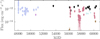Fig. A.3

Example for Fig. A.3 in Kaltenbrunner (2025). Long-term light curve extracted as explained in Sect. 5.4.2 for #10. The flux values and upper limits are shown for XMM-Newton Slew (black), XMM-Newton Pointed (dark yellow), Swift-XRT (salmon), ROSAT Pointed-HRI (plum), ROSAT Pointed-PSPC (light steel blue) and eROSITA (azure).

Table A.3

eRASS1 DETUIDs.

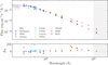Fig. B.1

Example for Fig. B.1 in Kaltenbrunner (2025). SED fits as described in Sect. 4.6 for #16. Coloured points show data from the different instruments, black points are model predictions convolved with the corresponding filters. Only data below 10 micron were used for the fit.

Appendix B SED fitting

Figure B.1 in Kaltenbrunner (2025) shows the results from SED fitting as explained in Sect. 4.6 for all sources listed as candidates in our sample. An example plot can be seen in Fig. B.1. Sources we flag to have an IR excess fit well for wavelengths below 10 microns and show overluminosity compared to the model prediction above. Table B.1 summarises the best-fit results we obtained. For 1eRASS J050945.8−655237 (#38), 1eRASS J055318.4−655953 (#49), 1eRASS J055536.1−671444 (#50), and 1eRASS J060212.5−674305 (#52), spectral fitting was unsuccessful, with inferred temperatures lower than expected for Be stars. This makes their classification as HMXBs uncertain. In the cases of 1eRASS J045028.2−693558 (#31) and 1eRASS J050053.3−653209 (#34), two distinct sources fall within the VizieR selection region and cannot be distinguished based on position alone. The spectral parameters presented in Table B.1 correspond to the object whose SED is consistent with that of a Be star, though the results – particularly the parameter uncertainties – should be taken with a grain of salt.

For sources for which optical spectra with SALT or LCO/FLOYDS were taken, Fig. B.2 shows a comparison of the best-fit result from SED fitting and the observed spectrum. This nicely shows the enhanced Hα flux.

Table B.1

SED fitting results.

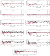Fig. B.2

Best-fit spectrum from SED fitting as described in Sect. 4.6 compared to LCO/FLOYDS spectrum for #28, #32, #35, #36, #37, #39, #41, #43, #44, #51 and #52.

Appendix C Gaia counterparts

Table C.1

Gaia DR3 counterparts of objects in our catalogue.

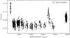Fig. D.1

Example for Fig. D.1 in Kaltenbrunner (2025). OGLE I-band light curves of stars with low-amplitude (<0.3 mag) variability.

Appendix D OGLE photometry

Our Fig. D.2 and Fig. D.1 in Kaltenbrunner (2025) (see Fig. D.1 for an example) present OGLE light curves of the systems investigated in this work.

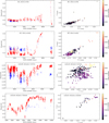Fig. D.2

OGLE photometry of highly variable stars (>0.3 mag in I). Left: OGLE I-band (red) and V-band (blue) light curves. Right: Colour (V−I) - magnitude (I) diagrams.

Table D.1

Periodicities in OGLE data.

All Tables

Table 1

Summary of spectroscopic observations done for objects in our catalogue.

In the text

Table 2

Catalogues used for matching (top) and screening of foreground and background sources (bottom).

In the text

Table 3

eRASS start and stop times.

In the text

Table 4

Model priors for the spectral fits.

In the text

Table 5

Known and candidate HMXB detected during eRASS1.

In the text

Table 6

Identification flags.

Confidence classes.

Rejected HMXB candidates.

In the text

Table 9

Best-fit results for Hβ and HeI 4921 lines for SALT spectra of 1eRASS J054422.3−672729.

In the text

Table 10

Best-fit parameters for CXOU J053600.0−673507.

In the text

Table A.1

Alternative names and literature references for discovery of the X-ray sources with confidence class 1 in our HMXB catalogue.

In the text

Table A.2

Same as Table A.1 for confidence classes 2−6.

eRASS1 DETUIDs.

SED fitting results.

Gaia DR3 counterparts of objects in our catalogue.

In the text

Table D.1

Periodicities in OGLE data.

In the text

All Figures

	Fig. 4 Flowchart summarising the selection process for new candidates included in the catalogue. A detailed description can be found in Sect. 3.2.
In the text

	Fig. 9 Short-term variability of AGN, HMXBs, and HMXB candidates represented by their var. For readability, the plot is capped at a maximum variability of 400. Six additional HMXBs exceed this var threshold, while no AGN or HMXB candidates show larger values.
In the text

	Fig. 12 Sensitivity function for eRASS 1 detection assuming a spectra defined by an absorbed power-law with power-law index 1 for three positions within the LMC (sky tile closest to SEP, sky tile in the centre of the LMC and sky tile most distant from the SEP) as well as the LMC average sensitivity.
In the text

	Fig. 15 OGLE phase-folded light curve of 1eRASS J054422.3−672729 with timing of the flares marked. Flares 1 and 2 refer to the flares at 373 and 730 days in Fig. 14, respectively.
In the text

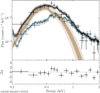	Fig. 18 Same as Fig. 17 but for 1eRASS J054242.7−672752 without local absorption.
In the text

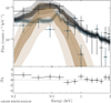	Fig. 19 Same as Fig. 17 but for 1eRASS J050705.9−652149 without local absorption.
In the text

	Fig. 20 EPIC-pn spectrum of 4XMM J053449.0−694338 with colours as in Fig. 17 visually rebinned for better readability.
In the text

Fig. 21

vapec

In the text

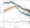	Fig. 22 Same as Fig. 20 but for RX J0516.0−6916.
In the text

Fig. 23

In the text

	Fig. 24 Radial velocity change of the blue component in the double-peaked Hα lines observed from XMMU J050722.1−684758 between 2008-11-28 and 2009-01-07 compared to a sinusoidal fit with a period frozen at the orbital period found with OGLE.
In the text

	Fig. 25 LS periodograms with highly significant peaks at periods below 10 d.
In the text

	Fig. 26 LS periodograms with peaks at longer periods.
In the text

	Fig. A.1 Example for Fig. A.1 in Kaltenbrunner (2025). Merged eROSITA spectrum with best fit models for #1. Black and blue data points are fluxes in the on- and off-region, respectively. Blue and yellow lines show the best-fit models for the background and source, the black line shows the sum of both. Shaded areas display the 1σ (dark) and 3σ (light) confidence for the models.
In the text

	Fig. A.2 Example for Fig. A.2 in Kaltenbrunner (2025). eROSITA light curve for #9. For readability white spaces between the individual eRASSs are removed. The light curves are rebinned to have a minimum number of 10 net source counts per time bin as described in Sect. 4.2.1. The variability var (found in the bottom right of each figure) is calculated as described in Sect 4.2.2.
In the text

	Fig. A.3 Example for Fig. A.3 in Kaltenbrunner (2025). Long-term light curve extracted as explained in Sect. 5.4.2 for #10. The flux values and upper limits are shown for XMM-Newton Slew (black), XMM-Newton Pointed (dark yellow), Swift-XRT (salmon), ROSAT Pointed-HRI (plum), ROSAT Pointed-PSPC (light steel blue) and eROSITA (azure).
In the text

	Fig. B.1 Example for Fig. B.1 in Kaltenbrunner (2025). SED fits as described in Sect. 4.6 for #16. Coloured points show data from the different instruments, black points are model predictions convolved with the corresponding filters. Only data below 10 micron were used for the fit.
In the text

	Fig. B.2 Best-fit spectrum from SED fitting as described in Sect. 4.6 compared to LCO/FLOYDS spectrum for #28, #32, #35, #36, #37, #39, #41, #43, #44, #51 and #52.
In the text

	Fig. D.1 Example for Fig. D.1 in Kaltenbrunner (2025). OGLE I-band light curves of stars with low-amplitude (<0.3 mag) variability.
In the text

	Fig. D.2 OGLE photometry of highly variable stars (>0.3 mag in I). Left: OGLE I-band (red) and V-band (blue) light curves. Right: Colour (V−I) - magnitude (I) diagrams.
In the text

Current usage metrics show cumulative count of Article Views (full-text article views including HTML views, PDF and ePub downloads, according to the available data) and Abstracts Views on Vision4Press platform.

Data correspond to usage on the plateform after 2015. The current usage metrics is available 48-96 hours after online publication and is updated daily on week days.

Initial download of the metrics may take a while.

[R1] Aidelman, Y., & Cidale, L. S. 2023, Galaxies, 11, 31 [NASA ADS] [CrossRef] [Google Scholar]

[R2] Antoniou, V., & Zezas, A. 2016, MNRAS, 459, 528 [Google Scholar]

[R3] Antoniou, V., Zezas, A., Hatzidimitriou, D., & Kalogera, V. 2010, ApJ, 716, L140 [NASA ADS] [CrossRef] [Google Scholar]

[R4] Arnaud, K. A. 1996, ASP Conf. Ser., 101, 17 [Google Scholar]

[R5] Assef, R. J., Stern, D., Noirot, G., et al. 2018, ApJS, 234, 23 [Google Scholar]

[R6] Astropy Collaboration (Robitaille, T. P., et al.) 2013, A&A, 558, A33 [NASA ADS] [CrossRef] [EDP Sciences] [Google Scholar]

[R7] Astropy Collaboration (Price-Whelan, A. M., et al.) 2018, AJ, 156, 123 [Google Scholar]

[R8] Astropy Collaboration (Price-Whelan, A. M., et al.) 2022, ApJ, 935, 167 [NASA ADS] [CrossRef] [Google Scholar]

[R9] Bailer-Jones, C. A. L., Fouesneau, M., & Andrae, R. 2019, VizieR Online Data Catalog: Gaia DR2 quasar and galaxy classification (Bailer-Jones+, 2019), VizieR On-line Data Catalog: VII/285 [Google Scholar]

[R10] Balona, L. A. 2000, ASP Conf. Ser., 214, 1 [Google Scholar]

[R11] Bamba, A., Ueno, M., Nakajima, H., Mori, K., & Koyama, K. 2006, A&A, 450, 585 [NASA ADS] [CrossRef] [EDP Sciences] [Google Scholar]

[R12] Bodensteiner, J., Sana, H., Dufton, P. L., et al. 2023, A&A, 680, A32 [NASA ADS] [CrossRef] [EDP Sciences] [Google Scholar]

[R13] Bonanos, A. Z., Lennon, D. J., Köhlinger, F., et al. 2010, AJ, 140, 416 [NASA ADS] [CrossRef] [Google Scholar]

[R14] Bozzo, E., Falanga, M., & Stella, L. 2008, ApJ, 683, 1031 [Google Scholar]

[R15] Brown, T. M., Baliber, N., Bianco, F. B., et al. 2013, PASP, 125, 1031 [Google Scholar]

[R16] Brunner, H., Liu, T., Lamer, G., et al. 2022, A&A, 661, A1 [NASA ADS] [CrossRef] [EDP Sciences] [Google Scholar]

[R17] Buchner, J. 2021a, J. Open Source Softw., 6, 3045 [NASA ADS] [CrossRef] [Google Scholar]

[R18] Buchner, J. 2021b, J. Open Source Softw., 6, 3001 [CrossRef] [Google Scholar]

[R19] Charles, P. A., Booth, L., Densham, R. H., et al. 1983, MNRAS, 202, 657 [NASA ADS] [Google Scholar]

[R20] Charles, P. A., Rajoelimanana, A., & Maccarone, T. J. 2011, ATel., 3751, 1 [Google Scholar]

[R21] Cioni, M. R. L., et al. 2023, VizieR Online Data Catalog: VISTA Magellanic Survey (VMC) catalog (YJKs) DR6 (Cioni+, 2011), VizieR On-line Data Catalog: II/375 [Google Scholar]

[R22] Cioni, M. R. L., Clementini, G., Girardi, L., et al. 2011, A&A, 527, A116 [CrossRef] [EDP Sciences] [Google Scholar]

[R23] Cioni, M. R. L., Kamath, D., Rubele, S., et al. 2013, A&A, 549, A29 [NASA ADS] [CrossRef] [EDP Sciences] [Google Scholar]

[R24] Coe, M. J., Negueruela, I., Buckley, D. A. H., Haigh, N. J., & Laycock, S. G. T. 2001, MNRAS, 324, 6234 [Google Scholar]

[R25] Coe, M. J., Finger, M., Bartlett, E. S., & Udalski, A. 2015, MNRAS, 447, 1630 [Google Scholar]

[R26] Coe, M. J., Kennea, J. A., Evans, P. A., & Udalski, A. 2020, MNRAS, 497, L50 [NASA ADS] [CrossRef] [Google Scholar]

[R27] Coe, M. J., Kennea, J. A., Monageng, I. M., et al. 2023, MNRAS, 524, 3263 [Google Scholar]

[R28] Corbet, R. H. D., Chomiuk, L., Coe, M. J., et al. 2016, ApJ, 829, 105 [Google Scholar]

[R29] Cowley, A. P., Crampton, D., Hutchings, J. B., Remillard, R., & Penfold, J. E. 1983, ApJ, 272, 118 [Google Scholar]

[R30] Cowley, A. P., Schmidtke, P. C., McGrath, T. K., et al. 1997, PASP, 109, 21 [NASA ADS] [CrossRef] [Google Scholar]

[R31] Crawford, D. F., Jauncey, D. L., & Murdoch, H. S. 1970, ApJ, 162, 405 [Google Scholar]

[R32] Crawford, S. M., Still, M., Schellart, P., et al. 2010, SPIE Conf. Ser., 7737, 773725 [Google Scholar]

[R33] de Wit, W. J., Lamers, H. J. G. L. M., Marquette, J. B., & Beaulieu, J. P. 2006, A&A, 456, 1027 [NASA ADS] [CrossRef] [EDP Sciences] [Google Scholar]

[R34] Dickey, J. M., & Lockman, F. J. 1990, ARA&A, 28, 215 [NASA ADS] [CrossRef] [Google Scholar]

[R35] Douna, V. M., Pellizza, L. J., Mirabel, I. F., & Pedrosa, S. E. 2015, A&A, 579, A44 [NASA ADS] [CrossRef] [EDP Sciences] [Google Scholar]

[R36] Dubus, G. 2006, A&A, 456, 801 [NASA ADS] [CrossRef] [EDP Sciences] [Google Scholar]

[R37] Ducci, L., Mereghetti, S., Santangelo, A., et al. 2022, A&A, 661, A22 [NASA ADS] [CrossRef] [EDP Sciences] [Google Scholar]

[R38] Esin, A. A., McClintock, J. E., & Narayan, R. 1997, ApJ, 489, 865 [NASA ADS] [CrossRef] [Google Scholar]

[R39] Evans, C. J., Taylor, W. D., Hénault-Brunet, V., et al. 2011, A&A, 530, A108 [NASA ADS] [CrossRef] [EDP Sciences] [Google Scholar]

[R40] Falanga, M., Bozzo, E., Lutovinov, A., et al. 2015, A&A, 577, A130 [NASA ADS] [CrossRef] [EDP Sciences] [Google Scholar]

[R41] Ferrigno, C., Bozzo, E., & Romano, P. 2022, A&A, 664, A99 [NASA ADS] [CrossRef] [EDP Sciences] [Google Scholar]

[R42] Flesch, E. W. 2023, VizieR Online Data Catalog: The Million Quasars (Milliquas) catalogue, version 8 (Flesch, 2023), VizieR On-line Data Catalog: VII/294 [Google Scholar]

[R43] Gaia Collaboration (Luri, X., et al.) 2021, A&A, 649, A7 [EDP Sciences] [Google Scholar]

[R44] Gamen, R., Barbà, R. H., Walborn, N. R., et al. 2015, A&A, 583, L4 [NASA ADS] [CrossRef] [EDP Sciences] [Google Scholar]

[R45] Goossens, M. E., Bird, A. J., Drave, S. P., et al. 2013, MNRAS, 434, 2182 [NASA ADS] [CrossRef] [Google Scholar]

[R46] Gordon, K. D., Clayton, G. C., Decleir, M., et al. 2023, ApJ, 950, 86 [CrossRef] [Google Scholar]

[R47] Greiner, J., Bornemann, W., Clemens, C., et al. 2008, PASP, 120, 405 [Google Scholar]

[R48] Grimm, H.-J., Gilfanov, M., & Sunyaev, R. 2003, Chinese J. Astron. Astrophys. Suppl., 3, 257 [Google Scholar]

[R49] Grundstrom, E. D., & Gies, D. R. 2006, ApJ, 651, L53 [NASA ADS] [CrossRef] [Google Scholar]

[R50] Haberl, F., & Pietsch, W. 1999a, A&AS, 139, 277 [Google Scholar]

[R51] Haberl, F., & Pietsch, W. 1999b, A&A, 344, 521 [NASA ADS] [Google Scholar]

[R52] Haberl, F., & Sturm, R. 2016, A&A, 586, A81 [NASA ADS] [CrossRef] [EDP Sciences] [Google Scholar]

[R53] Haberl, F., Pietsch, W., & Dennerl, K. 1995, A&A, 303, L49 [NASA ADS] [Google Scholar]

[R54] Haberl, F., Dennerl, K., Pietsch, W., & Reinsch, K. 1997, A&A, 318, 490 [Google Scholar]

[R55] Haberl, F., Dennerl, K., & Pietsch, W. 2003, A&A, 406, 471 [NASA ADS] [CrossRef] [EDP Sciences] [Google Scholar]

[R56] Haberl, F., Israel, G. L., Rodriguez Castillo, G. A., et al. 2017, A&A, 598, A69 [NASA ADS] [CrossRef] [EDP Sciences] [Google Scholar]

[R57] Haberl, F., Maitra, C., Carpano, S., et al. 2020a, ATel, 13609, 1 [Google Scholar]

[R58] Haberl, F., Maitra, C., Greiner, J., et al. 2020b, ATel, 13789, 1 [Google Scholar]

[R59] Haberl, F., Maitra, C., Greiner, J., et al. 2020c, ATel, 13709, 1 [Google Scholar]

[R60] Haberl, F., Wilms, J., Gokus, A., et al. 2020d, ATel, 13828, 1 [NASA ADS] [Google Scholar]

[R61] Haberl, F., Salganik, A., Maitra, C., et al. 2021, ATel, 15133, 1 [NASA ADS] [Google Scholar]

[R62] Haberl, F., Maitra, C., Vasilopoulos, G., et al. 2022, A&A, 662, A22 [NASA ADS] [CrossRef] [EDP Sciences] [Google Scholar]

[R63] Haberl, F., Maitra, C., Kaltenbrunner, D., et al. 2023, A&A, 671, A90 [NASA ADS] [CrossRef] [EDP Sciences] [Google Scholar]

[R64] Haberl, F., Xu, Y., Maitra, C., et al. 2025, MNRAS, 542, 583 [Google Scholar]

[R65] Hanuschik, R. W., Kozok, J. R., & Kaiser, D. 1988, A&A, 189, 147 [NASA ADS] [Google Scholar]

[R66] Harris, J., & Zaritsky, D. 2004, AJ, 127, 1531 [NASA ADS] [CrossRef] [Google Scholar]

[R67] Harris, J., & Zaritsky, D. 2009, AJ, 138, 1243 [NASA ADS] [CrossRef] [Google Scholar]

[R68] Hippke, M., David, T. J., Mulders, G. D., & Heller, R. 2019, AJ, 158, 143 [Google Scholar]

[R69] Hog, E., Fabricius, C., Makarov, V. V., et al. 2000, VizieR Online Data Catalog: The Tycho-2 Catalogue (Hog+ 2000), VizieR On-line Data Catalog: I/259 [Google Scholar]

[R70] Howarth, I. D. 2013, A&A, 555, A141 [NASA ADS] [CrossRef] [EDP Sciences] [Google Scholar]

[R71] Hutchings, J. B., Crampton, D., & Cowley, A. P. 1983, ApJ, 275, L43 [NASA ADS] [CrossRef] [Google Scholar]

[R72] Inam, S. Ç., Townsend, L. J., McBride, V. A., et al. 2009, MNRAS, 395, 1662 [Google Scholar]

[R73] in’t Zand, J. J. M. 2005, A&A, 441, L1 [CrossRef] [EDP Sciences] [Google Scholar]

[R74] Jain, C., Paul, B., & Dutta, A. 2009, MNRAS, 397, L11 [NASA ADS] [CrossRef] [Google Scholar]

[R75] Jansen, F., Lumb, D., Altieri, B., et al. 2001, A&A, 365, L1 [NASA ADS] [CrossRef] [EDP Sciences] [Google Scholar]

[R76] Jaxon, E. G., Guerrero, M. A., Howk, J. C., et al. 2001, PASP, 113, 1130 [Google Scholar]

[R77] Joss, P. C., & Rappaport, S. A. 1984, ARA&A, 22, 537 [Google Scholar]

[R78] Kahabka, P., de Boer, K. S., & Brüns, C. 2001, A&A, 371, 816 [NASA ADS] [CrossRef] [EDP Sciences] [Google Scholar]

[R79] Kahabka, P., Haberl, F., Payne, J. L., & Filipović, M. D. 2006, A&A, 458, 285 [NASA ADS] [CrossRef] [EDP Sciences] [Google Scholar]

[R80] Kaltenbrunner, D. 2025, A comprehensive catalogue of High-Mass Xray binaries in the Large Magellanic Cloud detected during the first eROSITA all-sky survey - Appendix Figures and Tables, available at DOI: 10.5281/zenodo.17833631 [Google Scholar]

[R81] Kaufer, A., Stahl, O., Tubbesing, S., et al. 1999, The Messenger, 95, 8 [Google Scholar]

[R82] Kennea, J. A., Coe, M. J., Evans, P. A., et al. 2020, ATel, 13823, 1 [Google Scholar]

[R83] Kennea, J. A., Coe, M. J., Evans, P. A., et al. 2021a, MNRAS, 508, 781 [NASA ADS] [CrossRef] [Google Scholar]

[R84] Kennea, J. A., Coe, M. J., Evans, P. A., et al. 2021b, ATel, 14341, 1 [Google Scholar]

[R85] Kim, D.-W., Protopapas, P., Trichas, M., et al. 2012, ApJ, 747, 107 [NASA ADS] [CrossRef] [Google Scholar]

[R86] Kovlakas, K., Zezas, A., Andrews, J. J., et al. 2021, MNRAS, 506, 1896 [NASA ADS] [CrossRef] [Google Scholar]

[R87] Kozłowski, S., & Kochanek, C. S. 2009, ApJ, 701, 508 [CrossRef] [Google Scholar]

[R88] Kozłowski, S., Onken, C. A., Kochanek, C. S., et al. 2013, ApJ, 775, 92 [CrossRef] [Google Scholar]

[R89] Krimm, H. A., Corbet, R. H. D., Evans, P. A., et al. 2009, ATel, 2011, 1 [Google Scholar]

[R90] Krimm, H. A., Barthelmy, S. D., Baumgartner, W., et al. 2013a, ATel, 5286, 1 [Google Scholar]

[R91] Krimm, H. A., Gelbord, J. M., Holland, S. T., & Kennea, J. A. 2013b, ATel, 5309, 1 [Google Scholar]

[R92] Krimm, H. A., Holland, S. T., & Kennea, J. A. 2013c, ATel, 5293, 1 [Google Scholar]

[R93] La Palombara, N., & Mereghetti, S. 2007, A&A, 474, 137 [NASA ADS] [CrossRef] [EDP Sciences] [Google Scholar]

[R94] La Palombara, N., Sidoli, L., Esposito, P., Tiengo, A., & Mereghetti, S. 2009, A&A, 505, 947 [NASA ADS] [CrossRef] [EDP Sciences] [Google Scholar]

[R95] La Palombara, N., Sidoli, L., Esposito, P., Tiengo, A., & Mereghetti, S. 2012, A&A, 539, A82 [NASA ADS] [CrossRef] [EDP Sciences] [Google Scholar]

[R96] Lanz, T., & Hubeny, I. 2003, ApJS, 146, 417 [NASA ADS] [CrossRef] [Google Scholar]

[R97] Lanz, T., & Hubeny, I. 2007, ApJS, 169, 83 [CrossRef] [Google Scholar]

[R98] Linden, T., Kalogera, V., Sepinsky, J. F., et al. 2010, ApJ, 725, 1984 [Google Scholar]

[R99] Liu, Q. Z., van Paradijs, J., & van den Heuvel, E. P. J. 2005, A&A, 442, 1135 [NASA ADS] [CrossRef] [EDP Sciences] [Google Scholar]

[R100] Liu, Q. Z., van Paradijs, J., & van den Heuvel, E. P. J. 2006, A&A, 455, 1165 [NASA ADS] [CrossRef] [EDP Sciences] [Google Scholar]

[R101] Lomb, N. R. 1976, Ap&SS, 39, 447 [Google Scholar]

[R102] Luck, R. E., Moffett, T. J., Barnes, T. G., III, & Gieren, W. P. 1998, AJ, 115, 605 [NASA ADS] [CrossRef] [Google Scholar]

[R103] Maggi, P., Haberl, F., Sturm, R., et al. 2013, A&A, 554, A1 [NASA ADS] [CrossRef] [EDP Sciences] [Google Scholar]

[R104] Maggi, P., Haberl, F., Kavanagh, P. J., et al. 2016, A&A, 585, A162 [NASA ADS] [CrossRef] [EDP Sciences] [Google Scholar]

[R105] Maitra, C., & Haberl, F. 2022, A&A, 657, A26 [NASA ADS] [CrossRef] [EDP Sciences] [Google Scholar]

[R106] Maitra, C., Haberl, F., Filipović, M. D., et al. 2019a, MNRAS, 490, 5494 [Google Scholar]

[R107] Maitra, C., Haberl, F., Ivanov, V. D., Cioni, M.-R. L., & van Loon, J. T. 2019b, A&A, 622, A29 [NASA ADS] [CrossRef] [EDP Sciences] [Google Scholar]

[R108] Maitra, C., Haberl, F., Carpano, S., et al. 2020a, ATel, 13610, 1 [Google Scholar]

[R109] Maitra, C., Haberl, F., Koenig, O., et al. 2020b, ATel, 13650, 1 [NASA ADS] [Google Scholar]

[R110] Maitra, C., Haberl, F., Maggi, P., et al. 2021a, MNRAS, 504, 326 [NASA ADS] [CrossRef] [Google Scholar]

[R111] Maitra, C., Haberl, F., Vasilopoulos, G., et al. 2021b, A&A, 647, A8 [NASA ADS] [CrossRef] [EDP Sciences] [Google Scholar]

[R112] Maitra, C., Haberl, F., Kaltenbrunner, D., et al. 2023a, ATel, 15886, 1 [NASA ADS] [Google Scholar]

[R113] Maitra, C., Kaltenbrunner, D., Haberl, F., et al. 2023b, A&A, 669, A30 [NASA ADS] [CrossRef] [EDP Sciences] [Google Scholar]

[R114] Maravelias, G., Zezas, A., Antoniou, V., & Hatzidimitriou, D. 2014, MNRAS, 438, 2005 [NASA ADS] [CrossRef] [Google Scholar]

[R115] Marino, A., Yang, H. N., Coti Zelati, F., et al. 2025, ApJ, 980, L36 [Google Scholar]

[R116] Mark, H., Price, R., Rodrigues, R., Seward, F. D., & Swift, C. D. 1969, ApJ, 155, L143 [NASA ADS] [CrossRef] [Google Scholar]

[R117] Martínez-Núñez, S., Kretschmar, P., Bozzo, E., et al. 2017, Space Sci. Rev., 212, 59 [Google Scholar]

[R118] Mateos, S., Alonso-Herrero, A., Carrera, F. J., et al. 2012, MNRAS, 426, 3271 [Google Scholar]

[R119] Mennickent, R. E., Pietrzyński, G., Gieren, W., & Szewczyk, O. 2002, A&A, 393, 887 [NASA ADS] [CrossRef] [EDP Sciences] [Google Scholar]

[R120] Merloni, A., Lamer, G., Liu, T., et al. 2024, A&A, 682, A34 [NASA ADS] [CrossRef] [EDP Sciences] [Google Scholar]

[R121] Meurs, E. J. A., & van den Heuvel, E. P. J. 1989, A&A, 226, 88 [NASA ADS] [Google Scholar]

[R122] Mirabel, I. F., & Rodríguez, L. F. 1998, Nature, 392, 673 [NASA ADS] [CrossRef] [Google Scholar]

[R123] Negueruela, I., & Coe, M. J. 2002, A&A, 385, 517 [NASA ADS] [CrossRef] [EDP Sciences] [Google Scholar]

[R124] Ochsenbein, F. 1996, The VizieR database of astronomical catalogues [Google Scholar]

[R125] Ochsenbein, F., Bauer, P., & Marcout, J. 2000, A&AS, 143, 23 [Google Scholar]

[R126] Orosz, J. A., Steeghs, D., McClintock, J. E., et al. 2009, ApJ, 697, 573 [NASA ADS] [CrossRef] [Google Scholar]

[R127] Orosz, J. A., Steiner, J. F., McClintock, J. E., et al. 2014, ApJ, 794, 154 [NASA ADS] [CrossRef] [Google Scholar]

[R128] Pasquini, L., Avila, G., Blecha, A., et al. 2002, The Messenger, 110, 1 [Google Scholar]

[R129] Pennock, C. M., van Loon, J. T., Filipovic, M. D., et al. 2021, VizieR Online Data Catalog: ASKAP-EMU ESP LMC Radio Continuum Survey (Pennock+, 2021), VizieR On-line Data Catalog: J/MNRAS/506/3540 [Google Scholar]

[R130] Pfahl, E., Rappaport, S., Podsiadlowski, P., & Spruit, H. 2002, ApJ, 574, 364 [Google Scholar]

[R131] Pietrzyński, G., Graczyk, D., Gallenne, A., et al. 2019, Nature, 567, 200 [Google Scholar]

[R132] Pols, O. R., Cote, J., Waters, L. B. F. M., & Heise, J. 1991, A&A, 241, 419 [NASA ADS] [Google Scholar]

[R133] Porter, J. M., & Rivinius, T. 2003, PASP, 115, 1153 [Google Scholar]

[R134] Predehl, P., Andritschke, R., Arefiev, V., et al. 2021, A&A, 647, A1 [EDP Sciences] [Google Scholar]

[R135] Raguzova, N. V. 2001, A&A, 367, 848 [NASA ADS] [CrossRef] [EDP Sciences] [Google Scholar]

[R136] Raguzova, N. V., & Popov, S. B. 2005, Astron. Astrophys. Trans., 24, 151 [Google Scholar]

[R137] Reid, N., Glass, I. S., & Catchpole, R. M. 1988, MNRAS, 232, 53 [Google Scholar]

[R138] Reig, P., & Nespoli, E. 2013, A&A, 551, A1 [NASA ADS] [CrossRef] [EDP Sciences] [Google Scholar]

[R139] Reig, P., & Roche, P. 1999, MNRAS, 306, 100 [NASA ADS] [CrossRef] [Google Scholar]

[R140] Remillard, R. A., & McClintock, J. E. 2006, ARA&A, 44, 49 [Google Scholar]

[R141] Richter, O. G., Tammann, G. A., & Huchtmeier, W. K. 1987, A&A, 171, 33 [Google Scholar]

[R142] Riquelme, M. S., Torrejón, J. M., & Negueruela, I. 2012, A&A, 539, A114 [NASA ADS] [CrossRef] [EDP Sciences] [Google Scholar]

[R143] Rivinius, T., Baade, D., & Štefl, S. 2003, A&A, 411, 229 [NASA ADS] [CrossRef] [EDP Sciences] [Google Scholar]

[R144] Rodrigo, C., & Solano, E. 2020, in XIV.0 Scientific Meeting (virtual) of the Spanish Astronomical Society, 182 [Google Scholar]

[R145] Rodrigo, C., Solano, E., & Bayo, A. 2012, SVO Filter Profile Service Version 1.0, IVOA Working Draft 15 October 2012 [Google Scholar]

[R146] Rolleston, W. R. J., Trundle, C., & Dufton, P. L. 2002, A&A, 396, 53 [NASA ADS] [CrossRef] [EDP Sciences] [Google Scholar]

[R147] Romano, P. 2015, J. High Energy Astrophys., 7, 126 [Google Scholar]

[R148] Sabogal, B. E., Mennickent, R. E., Pietrzyński, G., & Gieren, W. 2005, MNRAS, 361, 1055 [NASA ADS] [CrossRef] [Google Scholar]

[R149] Salganik, A., Tsygankov, S. S., Lutovinov, A. A., et al. 2022, MNRAS, 514, 4018 [NASA ADS] [CrossRef] [Google Scholar]

[R150] Sasaki, M., Haberl, F., & Pietsch, W. 2000, A&AS, 143, 391 [Google Scholar]

[R151] Savitzky, A., & Golay, M. J. E. 1964, Anal. Chem., 36, 1627 [Google Scholar]

[R152] Saxton, R. D., König, O., Descalzo, M., et al. 2022, Astron. Comput., 38, 100531 [NASA ADS] [CrossRef] [Google Scholar]

[R153] Scargle, J. D. 1982, ApJ, 263, 835 [Google Scholar]

[R154] Scargle, J. D. 1998, ApJ, 504, 405 [Google Scholar]

[R155] Scargle, J. D., Norris, J. P., Jackson, B., & Chiang, J. 2013a, ApJ, 764, 167 [Google Scholar]

[R156] Scargle, J. D., Norris, J. P., Jackson, B., & Chiang, J. 2013b, arXiv e-prints [arXiv:1304.2818] [Google Scholar]

[R157] Schmidtke, P. C., Cowley, A. P., Frattare, L. M., et al. 1994, PASP, 106, 843 [NASA ADS] [CrossRef] [Google Scholar]

[R158] Schmidtke, P. C., Cowley, A. P., Hauschildt, P. H., et al. 1996, PASP, 108, 668 [Google Scholar]

[R159] Secrest, N. J., Dudik, R. P., Dorland, B. N., et al. 2015, ApJS, 221, 12 [NASA ADS] [CrossRef] [Google Scholar]

[R160] Sen, K., Xu, X. T., Langer, N., et al. 2021, A&A, 652, A138 [NASA ADS] [CrossRef] [EDP Sciences] [Google Scholar]

[R161] Sen, K., El Mellah, I., Langer, N., et al. 2024, A&A, 690, A256 [NASA ADS] [CrossRef] [EDP Sciences] [Google Scholar]

[R162] Seward, F. D., Charles, P. A., Foster, D. L., et al. 2012, ApJ, 759, 123 [Google Scholar]

[R163] Shakura, N. I., & Sunyaev, R. A. 1973, A&A, 24, 337 [NASA ADS] [Google Scholar]

[R164] Shakura, N., Postnov, K., Kochetkova, A., & Hjalmarsdotter, L. 2012, MNRAS, 420, 216 [Google Scholar]

[R165] Shtykovskiy, P., & Gilfanov, M. 2005a, A&A, 431, 597 [NASA ADS] [CrossRef] [EDP Sciences] [Google Scholar]

[R166] Shtykovskiy, P., & Gilfanov, M. 2005b, MNRAS, 362, 879 [NASA ADS] [CrossRef] [Google Scholar]

[R167] Sidoli, L., Paizis, A., & Mereghetti, S. 2006, A&A, 450, L9 [NASA ADS] [CrossRef] [EDP Sciences] [Google Scholar]

[R168] Sidoli, L., Ponti, G., Sguera, V., & Esposito, P. 2023, A&A, 671, A150 [NASA ADS] [CrossRef] [EDP Sciences] [Google Scholar]

[R169] Skibba, R. A., Engelbracht, C. W., Aniano, G., et al. 2012, ApJ, 761, 42 [NASA ADS] [CrossRef] [Google Scholar]

[R170] Skowron, D. M., Skowron, J., Udalski, A., et al. 2021, ApJS, 252, 23 [Google Scholar]

[R171] Slettebak, A. 1988, PASP, 100, 770 [NASA ADS] [CrossRef] [Google Scholar]

[R172] Smith, D. M., Markwardt, C. B., Swank, J. H., & Negueruela, I. 2012, MNRAS, 422, 2661 [NASA ADS] [CrossRef] [Google Scholar]

[R173] Soria, R., Wu, K., Page, M. J., & Sakelliou, I. 2001, A&A, 365, L273 [NASA ADS] [CrossRef] [EDP Sciences] [Google Scholar]

[R174] Souchay, J., Gattano, C., Andrei, A. H., et al. 2019, VizieR Online Data Catalog: Astrometric Catalogue 5, LQAC-5 (Souchay+, 2019), VizieR On-line Data Catalog: J/A+A/624/A145 [Google Scholar]

[R175] Stan Development Team 2024, Stan Modeling Language Users Guide and Reference Manual v2.34, https://mc-stan.org/docs/reference-manual/ [Google Scholar]

[R176] Straizys, V., Lazauskaite, R., Liubertas, R., & Azusienis, A. 1998, Balt. Astron., 7, 605 [Google Scholar]

[R177] Strüder, L., Briel, U., Dennerl, K., et al. 2001, A&A, 365, L18 [Google Scholar]

[R178] Sturm, R., Haberl, F., & Pietsch, W. 2011a, ATel, 3747, 1 [Google Scholar]

[R179] Sturm, R., Haberl, F., & Pietsch, W. 2011b, ATel, 3753, 1 [Google Scholar]

[R180] Sturm, R., Haberl, F., Pietsch, W., et al. 2012a, A&A, 537, A76 [NASA ADS] [CrossRef] [EDP Sciences] [Google Scholar]

[R181] Sturm, R., Haberl, F., Pietsch, W., Immler, S., & Udalski, A. 2012b, ATel, 3993, 1 [Google Scholar]

[R182] Sturm, R., Haberl, F., Pietsch, W., et al. 2013, A&A, 558, A3 [NASA ADS] [CrossRef] [EDP Sciences] [Google Scholar]

[R183] Sun, N.-C., de Grijs, R., Subramanian, S., et al. 2017, ApJ, 849, 149 [Google Scholar]

[R184] Sunyaev, R., Arefiev, V., Babyshkin, V., et al. 2021, A&A, 656, A132 [NASA ADS] [CrossRef] [EDP Sciences] [Google Scholar]

[R185] Treiber, H., Vasilopoulos, G., Bailyn, C. D., et al. 2021, MNRAS, 503, 6187 [CrossRef] [Google Scholar]

[R186] Treiber, H., Vasilopoulos, G., Bailyn, C. D., Haberl, F., & Udalski, A. 2025, A&A, 694, A43 [NASA ADS] [CrossRef] [EDP Sciences] [Google Scholar]

[R187] Turner, M. J. L., Abbey, A., Arnaud, M., et al. 2001, A&A, 365, L27 [CrossRef] [EDP Sciences] [Google Scholar]

[R188] Udalski, A. 2008, Acta Astron., 58, 187 [NASA ADS] [Google Scholar]

[R189] Udalski, A., Szymanski, M., Kaluzny, J., Kubiak, M., & Mateo, M. 1992, Acta Astron., 42, 253 [NASA ADS] [Google Scholar]

[R190] Udalski, A., Szymanski, M. K., Soszynski, I., & Poleski, R. 2008, Acta Astron., 58, 69 [NASA ADS] [Google Scholar]

[R191] Udalski, A., Szymański, M. K., & Szymański, G. 2015, Acta Astron., 65, 1 [NASA ADS] [Google Scholar]

[R192] Valenti, S., Dand, D., & Howell, D. A. 2013, FLOYDS Manual and Pipeline, https://www.authorea.com/users/598/articles/6566 [Google Scholar]

[R193] van Jaarsveld, N., Buckley, D. A. H., McBride, V. A., et al. 2018, MNRAS, 475, 3253 [Google Scholar]

[R194] Vasilopoulos, G. 2025, A&A, 698, A26 [NASA ADS] [CrossRef] [EDP Sciences] [Google Scholar]

[R195] Vasilopoulos, G., Maggi, P., Haberl, F., et al. 2013a, A&A, 558, A74 [NASA ADS] [CrossRef] [EDP Sciences] [Google Scholar]

[R196] Vasilopoulos, G., Sturm, R., Haberl, F., Maggi, P., & Udalski, A. 2013b, ATel, 5540, 1 [Google Scholar]

[R197] Vasilopoulos, G., Haberl, F., Sturm, R., Maggi, P., & Udalski, A. 2014, A&A, 567, A129 [NASA ADS] [CrossRef] [EDP Sciences] [Google Scholar]

[R198] Vasilopoulos, G., Zezas, A., Antoniou, V., & Haberl, F. 2017, MNRAS, 470, 4354 [NASA ADS] [CrossRef] [Google Scholar]

[R199] Vasilopoulos, G., Maitra, C., Haberl, F., Hatzidimitriou, D., & Petropoulou, M. 2018, MNRAS, 475, 220 [Google Scholar]

[R200] Vasilopoulos, G., Ray, P. S., Gendreau, K. C., et al. 2020, MNRAS, 494, 5350 [NASA ADS] [CrossRef] [Google Scholar]

[R201] Walter, R., Lutovinov, A. A., Bozzo, E., & Tsygankov, S. S. 2015, A&A Rev., 23, 2 [Google Scholar]

[R202] White, N. E., & Marshall, F. E. 1984, ApJ, 281, 354 [Google Scholar]

[R203] Willingale, R., Starling, R. L. C., Beardmore, A. P., Tanvir, N. R., & O’Brien, P. T. 2013, MNRAS, 431, 394 [Google Scholar]

[R204] Wilms, J., Allen, A., & McCray, R. 2000, ApJ, 542, 914 [Google Scholar]

[R205] Yang, H. N., Maitra, C., Vasilopoulos, G., et al. 2025, MNRAS, 536, 1357 [Google Scholar]

[R206] Yeung, M. C. H., Freyberg, M. J., Ponti, G., et al. 2023, A&A, 676, A3 [NASA ADS] [CrossRef] [EDP Sciences] [Google Scholar]

[R207] Zaritsky, D., Harris, J., Thompson, I. B., Grebel, E. K., & Massey, P. 2002, AJ, 123, 855 [Google Scholar]

[R208] Zaritsky, D., Harris, J., Thompson, I. B., & Grebel, E. K. 2004, AJ, 128, 1606 [Google Scholar]