The inside-out quenching of the MHONGOOSE galaxy NGC 1371

S. Veronese; W. J. G. de Blok; F. Fraternali; F. M. Maccagni; J. Healy; D. Kleiner; T. A. Oosterloo; R. Morganti

doi:10.1051/0004-6361/202555735

Home

All issues

Volume 703 (November 2025)

A&A, 703 (2025) A249

Full HTML

Open Access

Issue		A&A Volume 703, November 2025


Article Number		A249
Number of page(s)		25
Section		Extragalactic astronomy
DOI		https://doi.org/10.1051/0004-6361/202555735
Published online		19 November 2025

A&A, 703, A249 (2025)

The inside-out quenching of the MHONGOOSE galaxy NGC 1371

S. Veronese¹^,2^⋆, W. J. G. de Blok¹^,2^,3, F. Fraternali², F. M. Maccagni⁴, J. Healy⁵^,6, D. Kleiner¹, T. A. Oosterloo¹^,2 and R. Morganti¹^,2

¹ Netherlands Institute for Radio Astronomy (ASTRON), Oude Hoogeveensedijk 4, 7991 PD Dwingeloo, The Netherlands
² Kapteyn Astronomical Institute, University of Groningen, PO Box 800 9700 AV Groningen, The Netherlands
³ Department of Astronomy, University of Cape Town, Private Bag X3, 7701 Rondebosch, South Africa
⁴ INAF – Osservatorio Astronomico di Cagliari, Via della Scienza 5, 09047 Selargius, CA, Italy
⁵ Jodrell Bank Centre for Astrophysics, School of Physics and Astronomy, University of Manchester, Oxford Road, Manchester M13 9PL, UK
⁶ United Kingdom SKA Regional Centre (UKSRC), University of Manchester, Oxford Road, Manchester M13 9PL, UK

^⋆ Corresponding author: veronese.astro@gmail.com

Received: 30 May 2025
Accepted: 19 September 2025

Abstract

We present the deepest 21 cm spectral line and 1.4 GHz broad-band continuum observations of nearby early-type spiral galaxy NGC 1371 as part of the MeerKAT H I Observations of Nearby Galactic Objects: Observing Southern Emitters (MHONGOOSE) survey. We found the neutral atomic hydrogen (H I) mostly distributed in a regularly rotating disk with a hole ∼5 kpc wide around the galactic centre. The continuum observations reveal, within the H I hole, emission from one of the lowest luminosity AGNs known to date and from two unique ∼10 kpc wide bipolar bubbles never observed before in this galaxy. The properties of the bubbles suggest that they may result from the impact of the low-power radio jet propagating within the gaseous disk instead of perpendicular to it. We found indication for jet-induced ionised outflows within the H I hole but no molecular gas (upper limit of M_H₂ < 2 × 10⁵ M_⊙) was detected. The emerging picture is that the gas in the central regions was rapidly depleted by the stellar bar or, despite its low power, the AGN in NGC 1371 is efficiently heating and/or removing the gas through the jets and possibly by radiative winds, leading to the inside-out quenching of the galaxy.

Key words: methods: observational / techniques: interferometric / galaxies: active / galaxies: Seyfert

© The Authors 2025

Open Access article, published by EDP Sciences, under the terms of the Creative Commons Attribution License (https://creativecommons.org/licenses/by/4.0), which permits unrestricted use, distribution, and reproduction in any medium, provided the original work is properly cited.

This article is published in open access under the Subscribe to Open model. Subscribe to A&A to support open access publication.

1. Introduction

There is a general consensus that galaxy formation and evolution are governed by two major physical processes: gas accretion (see reviews by Putman et al. 2012; Tumlinson et al. 2017; Péroux & Howk 2020; Tacconi et al. 2020; Faucher-Giguère & Oh 2023) and feedback (see reviews by Fabian 2012; Heckman & Best 2014; Harrison et al. 2018; Tacconi et al. 2020). The timescale for the depletion of gas in galaxies is less than a Hubble time (Saintonge et al. 2013, 2016; Tacconi et al. 2013; Saintonge & Catinella 2022), which requires gas accretion to explain the measured cosmic star formation history (Fraternali & Tomassetti 2012; Madau & Dickinson 2014; Davé et al. 2017; Walter et al. 2020; Chen et al. 2021), while feedback is needed to regulate the growth of galaxies (Silk & Mamon 2012; Somerville & Davé 2015). It is not known in detail how these two mechanisms interact throughout the lifetime of the Universe to assemble galaxies and produce the diversity of structures that we observe at the present age.

In our current understanding of gas accretion, pristine gas from the cosmic web or from the galaxy halo and mergers supplies the fuel for star formation over cosmic time. How this gas accretion occurs is an open question from both a theoretical and an observational perspective. One expectation is that for low-mass galaxies (halo mass < 5 × 10¹¹ M_⊙) it happens in a cold mode (Kereš et al. 2005, 2009; Dekel & Birnboim 2006; Dekel et al. 2009; van de Voort et al. 2011; Danovich et al. 2015; Nelson et al. 2016), where clouds and filamentary streams of cold gas (T < 10⁵ K) funnel onto galaxies and fuel the star formation. Conversely, high-mass galaxies are expected to be fed by hot-mode accretion, in which the gas falling onto galaxies forms a hot circumgalactic medium (CGM). This happens when the cooling time of the gas is greater than the free-fall time. When a hot CGM is formed, it can further cool through cooling flows (Thompson et al. 2016; Schneider et al. 2018, 2020; Fielding & Bryan 2022), thermal instabilities (McCourt et al. 2012; Sharma et al. 2012; Gaspari et al. 2018), and induced cooling (Fraternali & Binney 2006; Fraternali 2017; Marinacci et al. 2010, 2011; Li et al. 2021; Marasco et al. 2022). It is unclear whether most of the accretion occurs in a cold or hot phase; observationally, direct unambiguous evidence of gas accretion for the hot and the cold modes is still missing (Braun & Thilker 2004; Wolfe et al. 2013, 2016; Das et al. 2020, 2024; Kamphuis et al. 2022; Xu et al. 2022; Liu et al. 2023).

If our understanding of gas accretion is limited, this also applies to our knowledge of feedback. Feedback comes in two forms: stellar (Tacconi et al. 2020) and active galactic nuclei (AGNs; Fabian 2012; Heckman & Best 2014; Harrison et al. 2018). Stellar feedback acts as a regulator of star formation (Schaye 2004; Krumholz et al. 2009; Ostriker et al. 2010; Davé et al. 2012; Lilly et al. 2013; Leroy et al. 2013; Peng & Maiolino 2014; Somerville & Davé 2015; Hayward & Hopkins 2017; Tabatabaei et al. 2018). When star formation is high, supernova explosions inject energy into the galaxy, heat the interstellar medium (ISM), and expel gas from the galaxy via winds. This leads to the suppression of future star-forming activities. As star formation terminates, gas falls back onto the galaxy, cools down and collapses, restarting the stellar production. However, many of the details of this process are still uncertain, and recent observational (Samal et al. 2014; Egorov et al. 2017) and theoretical (Yu et al. 2020; Egorov et al. 2023) studies have proposed that supernova feedback may also be positive, locally enhancing the star formation rate.

The role of AGN feedback is also uncertain. It is invoked in cosmological simulation to quench star formation and supermassive black hole (SMBH) growth to match the predicted properties of massive galaxies (Schaye et al. 2015; Khandai et al. 2015; Dubois et al. 2016; McCarthy et al. 2017; Nelson et al. 2018; Davé et al. 2019). From a physical point of view, this negative feedback arises from the strong winds and jets launched by the central engine (Di Matteo et al. 2005; Springel et al. 2005; Bower et al. 2006; Croton 2006; Ciotti et al. 2010; Wagner et al. 2012; Pontzen et al. 2017; Zinger et al. 2020). These outflows blow out and heat the gas, preventing its cooling and collapse and suppressing star formation. However, some theoretical studies propose that AGN feedback may also have a positive effect, promoting star formation (Ishibashi & Fabian 2012; Zinn et al. 2013; Silk 2013; Mukherjee et al. 2018a). This happens because the jet winds compress and shock-heat the gas, which allows very efficient radiative cooling. Empirically, both negative and positive AGN feedback have been observed in a number of different galaxies (see e.g. Marasco et al. 2020; Venturi et al. 2021; Kondapally et al. 2023; Heckman & Best 2023; Heckman et al. 2024 for negative feedback and Santoro et al. 2015a; Cresci et al. 2015a,b; Gallagher et al. 2019; Zhuang & Ho 2020 for AGN-induced star formation), making our understanding of AGN feedback more ambiguous.

Both stellar and AGN feedback effects may be constrained by observational neutral atomic hydrogen (H I) studies (see Tamburro et al. 2009; Ostriker et al. 2010; Ianjamasimanana et al. 2012; Stilp et al. 2013; Kim & Oh 2022 for stellar feedback, Morganti et al. 2003, 2016; Morganti & Oosterloo 2018; Gupta et al. 2006; Chandola et al. 2011; Mahony et al. 2013; Geréb et al. 2015; Maccagni et al. 2017 for AGN feedback), and yet these studies are limited by the need for both column density sensitivity and angular and spectral resolution. The recent MeerKAT H I Observations of Nearby Galactic Objects: Observing Southern Emitters (MHONGOOSE, de Blok et al. 2024) survey represents a major step forward in understanding gas accretion and feedback in the context of galaxy formation and evolution. Using the high column density sensitivity (down to a few times 10¹⁷ cm⁻²), angular resolution (up to 7″), spectral resolution (1.4 km s⁻¹), and wide-field coverage (1.5°) of the MeerKAT radio telescope¹ (Jonas & MeerKAT Team 2016), MHONGOOSE studies the distribution and dynamics of H I in and around 30 nearby star-forming galaxies. We refer to de Blok et al. (2024) for information on MHONGOOSE and its selection criteria.

In this paper, we discuss the MHONGOOSE galaxy NGC 1371, a nearby early-type spiral galaxy member of the Eridanus group (Brough et al. 2006; For et al. 2023) (see Table 1 for the main observational properties). With a stellar mass of 4.3 × 10¹⁰ M_⊙ and a combined mid-IR and UV star formation rate (SFR) of 0.24 M_⊙ yr⁻¹ (Cluver et al. 2025), it is the only target in the MHONGOOSE sample that is significantly below the main sequence of galaxy star formation (de Blok et al. 2024), with a SFR that is ∼1.7 M_⊙ yr⁻¹ lower than expected. This statement holds even when considering different SFR estimates (Grundy et al. 2023). Photometric measurements of the λ ∼ 154 nm far-ultraviolet (FUV) and λ ∼ 623 nm (r) emission from the Galaxy Evolution Explorer (GALEX; Martin et al. 2005) and the Dark Energy Survey (DES; Dark Energy Survey Collaboration 2016) place this galaxy at the edge between the star-forming main sequence and the green valley.

Table 1.

NGC 1371 main observational properties.

It is unclear whether NGC 1371 hosts an AGN. Based on the Hα emission, Hameed & Devereux (1999) claimed that the nuclear ISM is probably heated by the ionising UV radiation from post-asymptotic giant branch stars rather than by AGN activity. The lack of nuclear activity was corroborated by Cisternas et al. (2013), who analysed the central X-ray emission with the Chandra X-ray Observatory (Weisskopf et al. 2000). However, based on the same Chandra observations, Hughes et al. (2007) asserts that the Hα-X-ray luminosity correlation in the NGC 1371 nucleus is compatible with the relation found for the AGN by Ho et al. (2001), suggesting that this galaxy hosts a low-luminosity AGN. Studying the ∼1.4 GHz continuum with the Giant Metrewave Radio Telescope (GMRT; Swarup 1990) Omar & Dwarakanath (2005) also claimed that NGC 1371 hosts an AGN. Evidence for this is a radio excess with respect to the far-infrared emission (Yun et al. 2001), the observation of a bright radio source coincident with the nuclear Hα emission, and a kiloparsec-scale jet-like structure with no Hα correspondence, suggesting that the extended radio emission does not come from star-forming regions. These findings are corroborated by Grundy et al. (2023) using the more sensitive and higher resolution 1.4 GHz continuum observation from the Widefield ASKAP L-band Legacy All-sky Blind surveY (WALLABY; Koribalski et al. 2020). This means that NGC 1371 is one of the most tantalising MHONGOOSE galaxies for the study of the effect of stellar and AGN feedback and possible quenching mechanisms. For example, environmental effects such as tidal interaction and gas stripping (see Hirschmann et al. 2014; Hatfield & Jarvis 2017 for theoretical works and Peng et al. 2015; Knobel et al. 2015 for observational evidence), as well as secular processes such as bar quenching (Khoperskov et al. 2018; George et al. 2019) or disk instabilities (Bluck et al. 2022) may suppress its star formation.

This paper is organised as follows. In Sect. 2 we present the MHONGOOSE data used in this study. In Sect. 3 we describe how these data were analysed to derive the main H I and radio properties of this galaxy. In Sect. 4 we discuss the results, focussing on the feedback mechanism that led to the suppression of star formation. In Sect. 5 we summarise our conclusions and briefly provide some future prospects.

2. Description of the data

2.1. H I observations

Detailed information on the MHONGOOSE H I observations is given in de Blok et al. (2024). In short, each galaxy is observed for a total of 55 hours, split into ten 5.5-hour sessions. For NGC 1371 we have an additional 5.5 hour track. The eleven tracks underwent the same calibration procedure and were combined as described in de Blok et al. (2024). For the H I, we used the 32k narrow-band data, consisting of 32 768 channels, each 3.265 kHz wide, giving a total bandwidth of 107 MHz. We binned the channels by 2, leading to a final velocity resolution of1.4 km s⁻¹.

The calibration was done with the Containerized Automated Radio Astronomy Calibration (CARAcal) pipeline (Józsa et al. 2020), which provides an all-in-one package to perform standard data reduction steps such as data flagging, calibration, continuum subtraction, and spectral line imaging. WSClean (Offringa et al. 2014; Offringa & Smirnov 2017) within the CARAcal environment cleaned the H I data iteratively using cleaning masks at progressively higher angular resolution, providing six H I cubes spanning a range of angular resolution, from 7″ to 90″. All cubes have a spectral resolution of 1.4 km s⁻¹ and cover a field of view of 1.5°.

In this work we aim to investigate the effects of stellar and AGN feedback across the disk, thus, we mainly used a high-resolution cube (beam: 13.7″ × 9.6″), created with a robust parameter r = 0.5 and without u-v tapering. The cube spans a range of ∼1000 km s⁻¹ centred on 1456.4 km s⁻¹, the central velocity of the galaxy and reaches a 3σ limiting column density of 1.1 × 10¹⁹ cm⁻² over 16 km s⁻¹, where σ = 1.1 × 10¹⁸ cm⁻² is the noise level.

2.2. 1.4 GHz continuum

In parallel with the 32k narrow-band data, observations were also obtained using the 4k-correlator mode with the same integration times. We use these to create a deep 1.4 GHz continuum image. The 4k data consist of 4096 channels with a channel width of 208.984 kHz, thus providing a bandwidth of 856 MHz centred on a frequency of 1284 MHz. Only the frequency range from 856–1650 MHz was considered (due to the drop-off of sensitivity towards the band edges).

The 4k-data were also reduced with CARAcal following standard calibration and flagging procedures. In the 910–950 MHz and 1510–1610 MHz bands all the data were flagged, while in the 1020–1060 MHz, 1080–1320 MHz and 1460–1500 MHz ranges about 60% of the data per channel were discarded. The 1408–1423 MHz band was additionally flagged to avoid bright H I emission. Channels were averaged by a factor five, and this averaged data set was used for three cycles of self-calibration within CARAcal. The resulting continuum measurement sets were combined and deconvolved with the oxkat package (Heywood 2020). This was also used to apply an additional direction-dependent calibration.

The wide bandwidth and long integration times make this observation one of the deeper continuum images made with MeerKAT of nearby galaxies, reaching a final noise level of 2.6 μJy at an angular resolution of 7.4″ × 6.7″ using a robust parameter r = 0. In Fig. 1, we present a multi-wavelength image of NGC 1371, incorporating several of the datasets discussed in this paper.

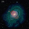Fig. 1.

Multi-wavelength image of NGC 1371. The background shows the combined gzri optical image from Dark Energy Camera Legacy Survey (DECaLS, Dey et al. 2019). The MeerKAT high-resolution 1.4 GHz radio continuum is shown in yellow and red. The UV emission as observed by GALEX is overlaid in pink. The multi-resolution H I from the MHOONGOOSE observations is given in green and blue.

2.3. Ancillary data

Beside the new MeerKAT observations, in this paper we used archival data from other facilities to study star formation and the possible AGN emission. Although H I can be seen as the gas reservoir for future star formation, it is molecular hydrogen (H₂), formed by cooling of H I clouds (Clark et al. 2012; Walch et al. 2015), which directly fuels stellar production (Meidt et al. 2015; Schinnerer et al. 2019; Walter et al. 2020). While H₂ itself is difficult to observe directly due to its lack of a permanent electric dipole moment, it can be traced by emission of carbon monoxide (CO) (Tacconi et al. 2013; Bolatto et al. 2013; Audibert et al. 2022, 2023) at millimetre wavelength. Therefore, we used Morita Atacama Compact Array (ACA; Iguchi et al. 2009) observations of NGC 1371 to trace the molecular ISM. These data were taken under the programme ID 2022.1.01314.S (PI: Adam Leroy). The bandwidth covers ∼500 km s⁻¹ centred on the CO_1 → 0 rest frequency ν_obs = 115.271 GHz. The FoV is a 93″ × 143″ (8.9 kpc × 13.7 kpc) rectangular mosaic around the major axis and centred on the galaxy.

The 1.4 GHz continuum is a tracer of the star formation (e.g. Cook et al. 2024), but it is sensitive to external contamination such as AGN. A more robust estimator of the SFR is therefore obtained by combining UV and infrared emission (Leroy et al. 2008). As such, we retrieved the Wide-field Infrared Survey Explorer (WISE; Wright et al. 2010) 12 μm (W3) and the GALEX FUV maps from Leroy et al. (2019) to quantify the current SFR of NGC 1371.

The H I and CO emission provides information on the colder phases of the ISM. For the most comprehensive view on what can cause the low SFR in NGC 1371 it is important to study also the hot gas. This is tracked by ionised atomic hydrogen (Hα) emission. Archival data are, however, restricted to the galactic centre. The available Hα observations come from integral field spectroscopy data taken by the Multi Unit Spectroscopic Explorer (MUSE; Bacon et al. 2010). MUSE observed the inner 5 kpc of the galaxy at ∼20-pc resolution under programme ID 108.227L.001 (PI: Peter Erwin). We retrieved the reduced data cube from the ESO Science Portal.

3. Data analysis

3.1. H I moment maps

In Fig. 2, we present, from left to right, the ∼10″-resolution H I intensity (moment-0), intensity-weighted mean velocity² (moment-1), and line-of-sight (LoS) velocity width (moment-2) map for NGC 1371, as derived by the Source Finding Application (SoFiA-2, Westmeier et al. 2021) using the parameters described in de Blok et al. (2024). The H I is distributed along tight spiral arms, with the outermost appearing to be disrupted. There is also a central H I hole with a diameter of ∼5 kpc. This hole is not due to absorption, as there is no significant negative flux within it, but rather to the absence of H I at the limiting column density of the map. This remains true even when inspecting the more sensitive, 30″ resolution data, which reach a 3σ limiting column density of 1.4 × 10¹⁸ cm⁻² over 16 km s⁻¹.

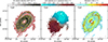Fig. 2.

High-resolution H I moment maps of NGC 1371. Left panel: Primary beam-corrected H I column-density map. The contour levels are given on the colour bar. In the bottom right we show the 13.7″ × 9.6″ beam. The 10 kpc reference scale is shown in the top left. Central panel: Intensity-weighted mean velocity field with respect to the systemic velocity (1456.4 km s⁻¹). The dashed contours refer to the approaching side, while the solid lines correspond to receding velocities. Right panel: moment 2 map, i.e. the velocity spread along each LoS. It corresponds to the velocity dispersion when the emission comes from a single line or to the spread of multiple components at different velocities.

The moment-1 map shows that most of the H I disk is undergoing regular rotation. The kinematic minor axis appears distorted, probably due to the warping of the outer disk. Nevertheless, other processes, such as radial motions and variations in the inclination angle, also affect the minor axis (Begeman 1987; Di Teodoro & Peek 2021). The kinematics at the edge of the H I hole is regular. In Fig. A.1 we show the 1250 km s⁻¹ to 1665 km s⁻¹ channel maps of the H I cube in steps of 28 km s⁻¹ to further illustrate the kinematical properties of the disk. These channel maps contain the H I intensity at a given velocity, providing an immediate visualisation of the gas rotation. The maps also clearly shows the H I hole. Furthermore, in Fig. 3 we include the position-velocity (pv) slices extracted³ along azimuthal angles of (0, 30, 60, 90, 120, 150) degrees, where 0 corresponds to the position angle of the major axis (φ = 135°). The pv diagram is a slice across the cube that gives the velocity of the gas as a function of a spatial coordinate, in this case the distance from the centre of the galaxy. Since the velocity of the gas along the LoS is given by (Begeman 1987)

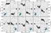Fig. 3.

Position-velocity diagrams at azimuthal angles (θ) of (0, 30, 60, 90, 120, 150) degrees with respect to the major axis in the plane of the sky. The data cube was spectrally smoothed with a 7 km s⁻¹ Hanning kernel. The solid contour levels denote the (4, 16, 64, 256, 1024)σ level, where σ = 0.03 mJy beam⁻¹. The dashed grey contours refers to the −4σ level. The dashed black horizontal line corresponds to the systemic velocity, while the dash-dotted black vertical line denotes the centre of the galaxy. The insets shows the moment 2 map and the slice along which the pv is extracted. The letters A and B provide the orientation in the main panels.

$\begin{matrix} v_{los} = v_{sys} + (v_{rot} cos θ + v_{rad} sin θ) sin i, \end{matrix}$ $\begin{aligned} v_{\rm los}=v_{\rm sys}+(v_{\rm rot}\cos {\theta }+v_{\rm rad}\sin {\theta })\sin {i}, \end{aligned}$ (1)

where v_sys, v_rad, and v_rot are the systemic, radial, and rotation velocity, respectively, while θ and i are the azimuthal and inclination angle, the pv along the major axis (θ = 0°, top left panel of Fig. 3) traces the rotation curve of the galaxy. Instead, along the minor axis (θ = 90°, bottom left panel of Fig. 3), non-circular motions can be identified via deviations from the systemic velocity. Intermediate values of θ allow for a complete overview of the gas kinematics.

In the upper right corner of the top left panel of Fig. 3 a significant clumpy emission is visible at ∼6′ from the galactic centre at a velocity of ∼1650 km s⁻¹. The H I mass of this object, that we refer to as MKT 033442-245148 (α = 3^h34^m42.31^s, δ = −24^d51^m47.52^s, cz = 1647 km s⁻¹), is M_H I = 6.6 × 10⁶ M_⊙. The overlay between the H I contours and the DECaLs gzri image presented in Fig. A.2 reveals that MKT 033442-245148 is likely a dwarf galaxy. Searching for known objects at the location of MKT 033442-245148 in the SIMBAD Astronomical Database (Wenger et al. 2000) and in the NASA/IPAC Extragalactic Database⁴ leads to no results. Therefore, MKT 033442-245148 is likely a new galaxy. An immediate question raising from this finding is whether this dwarf is interacting with NGC 1371. The moment maps of MKT 033442-245148, provided in Fig. A.3, show no clear signatures of tidal tails or gas stripping. The morphology and kinematics are fairly regular, with the only prominent feature being an asymmetry in the NE side of the galaxy. However, this asymmetry is also marginally resolved, therefore we do not consider it a strong indication of ongoing interaction between NGC 1371 and MKT 033442-245148. The above considerations holds even when inspecting the 30″ resolution data, suggesting that the > 10¹⁸ cm⁻² H I in this galaxy is relaxed.

The moment-2 map of NGC 1371 shows ∼15 km s⁻¹ values throughout the disk and > 15 km s⁻¹ around the H I hole along the minor axis of the disk and between the two spiral arms. However, interpreting these values is not straightforward, as they represent the velocity spread along the LoS: a high value can result from either a single structure with a large velocity width or multiple (narrow) components distributed along the LoS. To investigate this, we performed a detailed kinematical modelling of the H I disk with the 3D-Based Analysis of Rotating Objects via Line Observations (3D-Barolo, Di Teodoro & Fraternali 2015).

The modelling is performed via ‘tilted-ring’ fitting (Begeman 1987), where the disk is approximated in concentric rings. Each ring is parametrised with a set of five geometrical variables, namely, the rotation centroid (x₀, y₀), the position angle on the sky (PA), the inclination angle (i) and the scale height (z₀), and four kinematical parameters, that are the systemic, rotation, and radial velocity (v_sys, v_rot, v_rad) and the intrinsic velocity dispersion (σ₀) as a function of radius. For this fit we used the 3DFIT task of 3D-Barolo on the H I disk divided into rings with the width along the major axis equal to the beam (13.7″). The fitting procedure is a two-step process, described in detail in Di Teodoro & Peek (2021), where in the first step we constrained the rotation curve and in the second we fit the radial velocities (if present). This procedure is done on the approaching and receding side separately, as well as both sides simultaneously. To constrain the rotation curve we fixed the scale-height of the disk to 100 pc. Using different values is not critical: as long as they are between 0 and 1 kpc, differences in the best fit are negligible. As from Eq. (1) the radial velocities are minimal close to the major axis (θ = 0°), whereas v_rot has the larger contribution to v_los, we also fixed v_rad = 0 km s⁻¹ and set the weighting function for the fit to cos²(θ), such that the fit will focus on minimising the residuals along the major axis (Di Teodoro & Fraternali 2015). The minimisation is done on |model − data| to balance the residuals of the bright and faint emission (Di Teodoro & Fraternali 2015). The free parameter of the fit are, therefore, x₀, y₀, v_rot, v_sys, PA, i and the intrinsic dispersion σ₀. This first step consists furthermore in a two-stage fit. In the first stage, the free parameter are fitted. However, a systematic issue in the 3D modelling is that the fits of PA and i often show unrealistic scatter (Di Teodoro & Fraternali 2015). Thus, in the second stage of the fit 3D-Barolo regularises PA and i and repeats the fit on the free parameters. We chose Bezier functions (Di Teodoro & Fraternali 2015) for this regularisation, as we noticed that the radial profile of PA and i cannot be approximated by a constant or a simple polynomial. The result of this first, two-stage fit is used as prior for the second step, where we want to fit for radial motions. Equation (1) tells that the effect of v_rad is maximised along the minor axis (θ = 90°), whereas v_rot is now minimal. Consequently, any small error in the determination of v_rot has a minor impact in this step. We kept the best-fit values from the first step fixed and let v_rad free to vary. We also changed the weighting function to sin²(θ), as we want to minimise the residuals along the minor axis. Furthermore, in this step only the first stage of the fit is used, as PA andi are fixed.

In Fig. 4 we show the comparison of the radial profiles of the geometrical and kinematical parameters as derived by fitting only the receding (in magenta) and approaching side (in blue) or both sides simultaneously (in green). The differences in the best fits between the two sides are negligible. The jump in v_rot and σ₀ at 30 kpc correspond to the location of the outer spiral arm. Similarly, the difference in the H I surface density around 15 kpc is due to the asymmetry in the H I distribution of the inner disk. The parameter having the largest scatter among the three models is i. However, an unambiguous estimate for i is generally hard to achieve even with high-resolution, high S/N data (e.g. Di Teodoro & Peek 2021; Mancera Piña et al. 2022, 2024). Furthermore, comparing the model with the data using the same pv slices of Fig. 3 (see Figs. A.4, A.5 and A.6 in Appendix A) we found always a good agreement with the data.

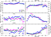Fig. 4.

Comparison of the best-fit parameters for the 3D model derived by 3D-Barolo fitting the approaching and receding side of the galaxy separately and simultaneously. From left to right and from top to bottom each panel shows v_rot, σ₀, v_rad, Σ_H I, i, and PA. The pink points refer to the best fit on the receding side, blue to the approaching side, and green to the simultaneous fit. The black horizontal dashed line in the v_rad panel is a visual guide indicating the 0-level, whereas in the i panel is the indicative optical inclination angle from NED (de Blok et al. 2024).

Hereafter we consider as the best-fit model the one derived from the simultaneous fit of both sides. This gives a constant centroid at (x₀, y₀) = (3^h 35^m 01.56^s, −24^d 56^m 00.12^s), almost identical to the fiducial position of (x₀, y₀) = (3^h 35^m 01.35^s, −24^d 55^m 59.58^s) listed in NED from WISE observations, and a constant systemic velocity of v_sys = 1456.4 km s⁻¹, the same value derived from the global profile (de Blok et al. 2024). This already indicates that the kinematics of this galaxy is gloablly regular, as there are no major disturbances able to shift the central velocity of the global profile away from v_sys. The radial velocities are consistent with 0 km s⁻¹ over the whole disk (⟨v_rad⟩= − 1.5 ± 3.9 km s⁻¹). In Fig. 5, we compare the observed moment-2 map with the one derived by 3D-Barolo using the aforementioned model. The high dispersion in the galactic centre is also present in the mock moment map, indicating that it is a resolution effect caused by the extremely steep rise on the rotation curve compared to the beam size.

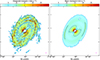Fig. 5.

Comparison between the observed (left) and mock (right) moment-2 map derived with 3D-Barolo. In the bottom right corner the 13.7″ × 9.6″ beam is displayed.

3.2. Radio continuum

In the left panel of Fig. 6 we present the radio continuum map. We detected⁵ a previously known jet-like structure (Omar & Dwarakanath 2005; Grundy et al. 2023), comprising of a core, two inner hotspots, and two outer hotspots. Due to the high sensitivity of MeerKAT, we also detect two (in projection) ∼10 kpc wide nuclear bubbles that have never been observed before in this galaxy. We used the process_image task of the Python Blob Detector and Source Finder⁶ (PyBDSF; Mohan & Rafferty 2015) to quantify the 1.4 GHz luminosity (L_1.4 GHz) of these structures and the galaxy as a whole. PyBDSF decomposes an image into a set of Gaussians and subsequently merges them into sources. These sources are then parametrised and recorded in a catalogue. The software also produces model and residual images for visual inspection, shown in the central and right panels of Fig. 6, respectively. The total luminosity of the entire jet-like structure, as derived by PyBDSF, is $L_{1.4 GHz}^{jet} = (9.75 \pm 0.04) \times 10^{20}$ $L^{\mathrm{jet}}_{1.4\,\mathrm{GHz}}=(9.75\pm0.04)\times10^{20}$ W Hz⁻¹, consistent with the measurements from the literature summarised in Table 1 of Grundy et al. (2023). The core alone has a luminosity of $L_{1.4 GHz}^{core} = (7.17 \pm 0.05) \times 10^{19}$ $L^{\mathrm{core}}_{1.4\,\mathrm{GHz}}=(7.17\pm0.05)\times10^{19}$ W Hz⁻¹.

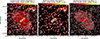Fig. 6.

1.4 GHz continuum maps. From left to right: Observed radio continuum, best-fit model from pPyBDSF, and the residuals in terms of data-model. The contour levels, with the lowest corresponding to 3σ, are given by the colour bar at the top. A 5 kpc reference line is given in the bottom left corner. In the central panel we indicate with blue arrows the locations of the core (C), the two inner hotspots (I), and the two outer hotspots (O). In the right panel we highlight the edge-brightening of the bubbles with the cyan dashed contours, corresponding to a flux density of 10 μJy beam⁻¹.

From the residual image, we also estimated the luminosity of the bubbles. We isolated them by applying an initial 3σ cut to the residual image (right panel of Fig. 6), followed by manual masking of the remaining low-level sources outside the bubbles. Summing the flux in the map yields $L_{1.4 GHz}^{bubbles} < 4.6 \times 10^{20}$ $L^{\mathrm{bubbles}}_{1.4\,\mathrm{GHz}} < 4.6\times10^{20}$ W Hz⁻¹, where the upper limit is to account for contamination by low-level background sources and residual faint emission from the jets or star-forming regions not included in the PyBDSF modelling. The total continuum luminosity of NGC 1371 is therefore L_1.4 GHz < 1.5 × 10²¹ W Hz⁻¹, placing the galaxy at the faint end of the 1.4 GHz luminosity function of radio galaxies, both observationally (Pracy et al. 2016; Butler et al. 2019) and theoretically (Thomas et al. 2021). In Table 2 we list the 1.4 GHz flux and luminosity for the various radio components.

Table 2.

NGC 1371 radio flux.

The high S/N of our data allows us to derive the spatially resolved distribution of the spectral index (α) in the 950–1408 MHz band, defined by the non-thermal power law S_ν ∝ ν^α, where S_ν is the monochromatic flux at frequency ν. We convolved the cube to the lowest-resolution beam and to avoid contamination of background sources, we used the PyBDSF model image (see the central panel of Fig. 6) to mask the LoS containing background quasars. Finally, we determined α using a fit⁷ to the logarithmic spectrum at each position. For each unmasked LoS, only channels with flux > 3σ were considered for the fit. The uncertainty on α (Δα) is computed from the covariance matrix of the best-fit parameters. Its distribution in terms of $\frac{Δ α}{α}$ $\frac{\Delta\alpha}{\alpha}$ is given in the right panel of Fig. 7. LoS for which $\frac{Δ α}{α} > 0.5$ $\frac{\Delta\alpha}{\alpha} > 0.5$ are shown in red and were further rejected from the spectral index map, presented in the left panel of Fig. 7.

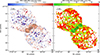Fig. 7.

Spatially resolved 950–1408 MHz spectral index map (left panel) and percentage uncertainty (right panel). The white regions in the left panel are due to the masking of contaminant sources and unreliable fits (see text for the details). The contour levels are given in the colour bar. In the right panel we show the percentage error on the spectral index in terms of $100 \cdot \frac{Δ α}{α}$ $100\cdot\frac{\Delta\alpha}{\alpha}$ , where Δα is the uncertainty on α as derived by the least-squares fit. The LoS where Δα > 50% are marked in red. These were removed from the map on the left. Contaminant sources are masked. In both maps, the black contours refers to the radio continuum from the jet (levels: 36, 141, 367, 772 μJy beam⁻¹), while the 7.4″ × 6.7″ beam is reported in the bottom right corner and a 5 kpc reference line is given in the top left corner.

3.3. Star formation rate density

The high spatial resolution of the MHONGOOSE observations allows for spatially resolved study of the correlation between the H I and radio continuum distribution with the SFR. Therefore, we computed SFR density maps (Σ_SFR) from the WISE W3 and the GALEX FUV data from Leroy et al. (2019), which already include masks for foreground stars. After correcting for the inclination of NGC 1371, we converted the FUV (I_FUV) and W3 (I_W3) intensities into Σ_SFR using the following equation, described in Leroy et al. (2019):

$\begin{matrix} \begin{matrix} \frac{Σ_{SFR}}{M_{⊙} {yr}^{- 1} {kpc}^{- 2}} = & 1.04 \times 10^{- 1} (\frac{C FUV}{10^{43.35}}) (\frac{I_{FUV}}{1 {MJy sr}^{- 1}}) \\ + 3.77 \times 10^{- 3} (\frac{C_{W 3}}{10^{42.79}}) (\frac{I_{W 3}}{1 {MJy sr}^{- 1}}) . \end{matrix} \end{matrix}$ $\begin{aligned} \begin{aligned} \frac{\Sigma _{\mathrm{SFR}}}{\mathrm{M}_\odot \,{\mathrm{yr}}^{-1}\,{\mathrm{kpc}}^{-2}}=&1.04\times 10^{-1}\left(\frac{C{\mathrm{FUV}}}{10^{43.35}}\right)\left(\frac{I_{\mathrm{FUV}}}{1\,\mathrm{MJy\,sr}^{-1}}\right)\\ &+3.77\times 10^{-3}\left(\frac{C_{\mathrm{W3}}}{10^{42.79}}\right)\left(\frac{I_{\mathrm{W3}}}{1\,\mathrm{MJy\,sr}^{-1}}\right) .\end{aligned} \end{aligned}$ (2)

Here C_FUV = 10^43.42 and C_W3 = 10^42.79 are the FUV and W3 correction factors, respectively. The resulting map is shown in Fig. 8.

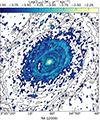Fig. 8.

Star formation density map derived with the prescription given in Leroy et al. (2019). The black contours correspond to H I column densities of (0.3, 2.9, 11.3, 29.5, 62.1) × 10¹⁹ cm^-2.

In Fig. 9 we overlay the radio continuum with the H I moment 0, the Σ_SFR map and the optical image from DECaLS. This immediate positional comparison shows that there is little-to-no spatial correlation between the radio continuum and the H I distribution. The lack of significant radio emission from the spiral arms is also qualitatively consistent with the low SFR of this galaxy and with the sparse distribution of star-forming regions in the UV imaging. Interestingly, the jet-like structure has no clear counterpart in both the Σ_SFR and optical image.

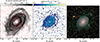Fig. 9.

Overlays of the H I (left), star formation density (center), and optical (right) map with the radio continuum contours. Contour levels are (0.006, 0.06, 0.2, 0.6, 1.3) mJy beam⁻¹, with the lowest being equivalent to 5σ. The optical image is an RGB composition of the gzri DECaLS observations.

4. Discussion

By analysing the H I and radio continuum emission, as well as Σ_SFR of NGC 1371, we found a jet-like structure within the central H I hole having a luminosity of $L_{1.4 GHz}^{jet} = (9.75 \pm 0.04) \times 10^{20}$ $L^{\mathrm{jet}}_{1.4\,\mathrm{GHz}}=(9.75\pm0.04)\times10^{20}$ W Hz⁻¹. This structure is not visible in the Σ_SFR and is more extended than the stellar bar. In the radio continuum we also detected previously unknown bipolar nuclear bubbles with a projected size of ∼10 kpc and luminosity of $L_{1.4 GHz}^{bubbles} < 4.6 \times 10^{20}$ $L^{\mathrm{bubbles}}_{1.4\,\mathrm{GHz}} < 4.6\times10^{20}$ W Hz⁻¹. In the following we discuss whether those features are attributed to the stellar bar or to an AGN or to both, and how they could explain the low SFR of the galaxy.

4.1. Determining whether NGC 1371 is an active galaxy

Whether NGC 1371 hosts an AGN is a matter of debate (see the discussion in Sect. 1). Our radio continuum data reveals the presence of a jet-like structure, already detected previously (Omar & Dwarakanath 2005; Grundy et al. 2023), that we can now study in more detail to understand if it is coming from an AGN or from the star formation in the stellar bar.

One way to distinguish between the two origins is to compare L_1.4 GHz with the SFR, as there is a well-known correlation between L_1.4 GHz and the SFR (Cook et al. 2024). From the Σ_SFR map derived earlier we measured a total SFR within the jet-like region of ∼0.03 M_⊙ yr⁻¹. The SFR-L_1.4 GHz relation from Cook et al. (2024) gives an estimation for L_1.4 GHz of 1.6 × 10¹⁹ W Hz⁻¹. This value is approximately 2 dex lower than $L_{1.4 GHz}^{jet}$ $L^{\mathrm{jet}}_{1.4\,\mathrm{GHz}}$ derived by PyBDSF. This suggests that star formation is unlikely to be responsible for the jet-like structure and that a low-luminosity AGN is the most probable cause.

Another parameter commonly used for distinguishing radio emission from star formation from that of AGN activity is the spectral index. The spectral index associated with star formation typically lies within the range −0.6 to −0.8 (Magnelli et al. 2015; Tabatabaei et al. 2017; Klein et al. 2018; An et al. 2021, 2024), whereas AGNs can exhibit a broader range of values (Eckart et al. 1986; Zajaček et al. 2019): spectral indices of α < −0.7 are characteristic of optically thin synchrotron emission from cool electrons in radio lobes, while −0.7 < α < −0.4 indicates a mixed contribution of optically thin and self-absorbed synchrotron emission from jets and values of α > −0.4 are typical of AGN cores, where synchrotron self-absorption becomes significant. From the spectral index map presented in Fig. 7 we measured an average spectral index in the radio core of α = −0.43 ± 0.01, consistent with the synchrotron self-absorption emission from an AGN core, while the radio emission from the jet has α < −0.7, which is consistent with the expected value for radio lobes. However, we must point out that our spectral index analysis has some caveats: the derivation of the spectral index strongly depends on the frequency range, the thermal contamination and the acceleration mechanism for the charged particles. Nonetheless, with the further support of the radio excess in the jet-like structure and the lack of similar features in the Σ_SFR map and the optical image, as shown in Fig. 9, we conclude that NGC 1371 is an active galaxy and the jet-like structure is tracing the AGN jet, rather than the star formation in thestellar bar.

4.2. Bubbles in other galaxies

Observations of disk galaxies hosting a radio AGN are rare (Ledlow et al. 1998; Abdo et al. 2009; Morganti et al. 2011; Doi et al. 2012; Bagchi et al. 2014; Singh et al. 2015). Kiloparsec-scale radio bubbles misaligned with the jets are even rarer, with only few known cases up to date (see Table 4 of Hota & Saikia 2006 and also Mrk 231, Ulvestad et al. 1999; M87, Owen et al. 2000; de Gasperin et al. 2012; The Teacup, Harrison et al. 2015; NGC 4438, Li et al. 2022 and M106, Zeng et al. 2023). Apart from The Teacup (undetermined morphology) and M87 (cD0-1 pec), all the aforementioned galaxies are classified as disc. Regarding the radio luminosity, NGC 4051 and M51 have L_1.4 GHz one dex lower than NGC 1371 (Hota & Saikia 2006), but their bubbles are also much smaller, with an estimated extent of 0.5 kpc. NGC 3367 has ∼15.3 kpc bipolar bubbles (Hota & Saikia 2006) but its radio emission (L_1.4 GHz = 1.12 × 10²² W Hz⁻¹) is much brighter than NGC 1371. The other galaxies have L_1.4 GHz two to three orders of magnitude higher than NGC 1371 and bubble sizes in the range of 1–3.4 kpc. Therefore, the bubbles of NGC 1371 have unique aspects.

4.3. Comparison with the Fermi/eROSITA bubbles

In our Galaxy 10 kpc bipolar nuclear bubbles have been detected at γ- and X-ray energies (reviewed by Sarkar 2024). The radio emission from the so-called ‘Fermi/eROSITA bubbles’ (FEBs) exhibits a northern loop whose outer edge closely follows the FEBs (Haslam et al. 1982; Kalberla et al. 2005; Planck Collaboration XXV 2016). There is an ongoing debate on whether this radio emission results from a nearby (∼200 pc away from us) supernova (e.g. Vidal et al. 2015; Dickinson 2018) or nuclear activity (e.g. Mou et al. 2014, 2015; Zhang & Guo 2020; Yang et al. 2022; Mondal et al. 2022). Arguments supporting the supernova origin arise from the absence of a southern FEBs radio counterpart, though some simulations suggest this could also result from nuclear activity interacting with an inhomogeneous CGM (e.g. Sarkar 2019). The question is whether the FEBs can provide insights into the properties of the bubbles in NGC 1371, and vice versa. In other words, we need to determine if the radio bubbles in NGC 1371 could be extragalactic analogues of the FEBs.

Unfortunately, there is no detected X-ray emission for the NGC 1371 bubbles (see Fig. 10), preventing a direct comparison. However, similarities can still be explored. Hughes et al. (2007) studied the X-ray distribution from NGC 1371 and found a compact source coincident with the nucleus and well described by an absorbed power-law spectrum with unabsorbed 0.5–10 keV flux of F_{2 − 10 keV} = 1.2 × 10⁻¹² erg cm⁻² s⁻¹. They also found diffuse emission in a 2.6 kpc × 1.3 kpc region around the galactic centre, coinciding with the radio jet (see the green ellipse in Fig. 10). The X-ray spectrum is consistent with thermal emission from a hot (kT ∼ 10 keV) and a warm (kT ∼ 0.3 keV) medium. The authors suggested that this emission originates from sources linked to recent star formation, but we argue that the X-rays likely trace the ISM heated by the jet, as they correlate well with the brightest radio continuum. Hughes et al. (2007) detected also very faint and soft diffuse emission (E < 2 keV) within an 8.6 kpc × 6.2 kpc region around the AGN (see the blue ellipse in Fig. 10), enclosing the radio lobes and the base of the bubbles. Notably, they report a medium temperature of ∼0.4 keV, similar to the FEBs (∼0.3 keV; Kataoka et al. 2013, 2018; Miller & Bregman 2016; Ursino et al. 2016).

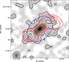Fig. 10.

Chandra X-ray image of NGC 1371. The X-ray emission has been smoothed with a Gaussian 1 kpc × 1 kpc kernel (given in the bottom right corner) to enhance the faint emission. The black contour denotes the 3σ level of the smoothed X-ray image. The red contours refers to the radio continuum (levels: 0.08, 0.31, 0.80, 1.68 mJy beam⁻¹, where the beam is 7.4″ × 6.7″). The dashed green and blue ellipses correspond to the extraction regions of the X-ray spectra studied by Hughes et al. (2007).

Since NGC 1371 is an active galaxy, it is possible that the bubbles are produced by its AGN. For this we further compare the nuclear activity of NGC 1371 with our Galaxy under the assumption that the FEBs are also ejected by our central SMBH, Sgr A^⋆. In fact, whether FEBs result from nuclear starburst or AGN activity remains debated (see Sarkar 2024, and references therein). Sgr A^⋆ has a mass of 4.14 × 10⁶ M_⊙ (Event Horizon Telescope Collaboration 2022a) (see also Gillessen et al. 2009; Davis et al. 2014), current accretion rate of 10⁻⁸–10⁻⁹ M_⊙ yr⁻¹ (Sharma et al. 2007; Event Horizon Telescope Collaboration 2022b; Ressler et al. 2023), and current bolometric luminosity of ∼10³⁶ erg s⁻¹ (Event Horizon Telescope Collaboration 2022b). In Table 3 we compare these quantities for Sgr A^⋆ and the SMBH in NGC 1371. Estimates in the literature for the mass of the SMBH in NGC 1371 (M_SMBH) already exist. From the spiral arm pitch angle Davis et al. (2014) derived M_SMBH = 10^{6.17 ± 0.5} M_⊙, close to Sgr A^⋆, but from the well-known M_SMBH − σ_⋆ relation (Woo et al. 2013), where σ_⋆ is the velocity dispersion of the stellar bulge, Cisternas et al. (2013) estimated M_SMBH ∼ 10^7.4 M_⊙, an order of magnitude higher than Sgr A^⋆. They also provided the bolometric luminosity (L_bol ∼ 8 × 10⁴¹ erg s⁻¹), from which we estimated the accretion rate (ṁ) onto the SMBH in NGC 1371 via

$\begin{matrix} \dot{m} = 1.59 \times 10^{- 26} \frac{L_{bol}}{ϵ c^{2}}, \end{matrix}$ $\begin{aligned} \dot{m} = 1.59\times 10^{-26}\frac{L_{\rm bol}}{\epsilon c^2} ,\end{aligned}$ (3)

Table 3.

Comparison of Sgr A^⋆ and the SMBH in NGC 1371.

where ϵ = 0.1 is the typical efficiency for the conversion of accreted mass into radiant energy (e.g. Heckman & Best 2014), c is the speed of light and 1.59 × 10⁻²⁶ is the conversion factor from g s⁻¹ to M_⊙ yr⁻¹. This gives $\dot{m} \sim 1.4 \times 10^{- 4}$ $\dot{m}\sim1.4\times10^{-4}$ M_⊙ yr⁻¹.

In conclusion, we do not find conclusive evidence that the bubbles in NGC 1371 are extragalactic analogous to the FEBs. They share a similar medium temperature and size, but there are some differences in the mass and activity of the SMBH. Nevertheless, this does not exclude that they are the same class of object.

4.4. The origin of the bubbles

Bipolar nuclear bubbles are typically produced by AGNs via jet-ISM interaction (see e.g. Morganti et al. 1998; Ulvestad et al. 1999; Owen et al. 2000; Hota & Saikia 2006; Harrison et al. 2015; Mukherjee et al. 2018a; Li et al. 2022; Yang et al. 2022; Tanner & Weaver 2022; Kondapally et al. 2023; Zeng et al. 2023) or by a burst of nuclear star formation (e.g. Baum et al. 1993; Su et al. 2010; Crocker & Aharonian 2011; Crocker et al. 2015; Yang et al. 2018; Bland-Hawthorn et al. 2019; Ponti et al. 2019; Meliani et al. 2024; Thompson & Heckman 2024). Determining whether they originate from AGN activity or star formation bursts is not straightforward for NGC 1371, given its low SFR and the uncertainty regarding their physical properties. From Fig. 7 we see that the bubbles have structures in the spectral index distribution. The inner part of the bubbles is dominated by the steep synchrotron emission from old, cooler electrons (α ≪ −0.7; e.g. Harwood et al. 2013), while on the edges the emitting medium is likely warmer, as the spectrum is flatter. Although the spectral index in the bubbles is inconsistent with the values for star-forming activity (−0.8 < α_SFR < −0.6), as mentioned in Sect. 4.1 our analysis has caveats that need to be taken into account. Thus, without a proper correction for the contamination by thermal emission and without an extension of the frequency range, not possible with the current data, we cannot rule out that the bubbles are the remnant of a past burst of star formation in the stellar bar.

Recent pc-resolution hydrodynamical simulations of the interaction between a P_jet < 10⁴⁵ erg s⁻¹ jet and the surrounding medium have shown that kiloparsec-scale bipolar bubbles, different from the radio lobes of the jet, are a natural consequence of the jet propagating within the gaseous disk at inclinations > 45° with respect to the rotational axis of the galaxy (Mukherjee et al. 2018a; Tanner & Weaver 2022).

With the P_jet − L_1.4 GHz relation from Heckman & Best (2014)

$\begin{matrix} Log (\frac{P_{jet}}{W}) = 4 \times 10^{35} {(f_{W})}^{\frac{3}{2}} Log {(\frac{L_{1.4 GHz}}{10^{25} {W Hz}^{- 1}})}^{0.86}, \end{matrix}$ $\begin{aligned} \mathrm{Log}\left(\frac{P_{\rm jet}}{\mathrm{W}}\right) = 4\times 10^{35}(f_W)^\frac{3}{2}\mathrm{Log}\left(\frac{L_{1.4\,\mathrm{GHz}}}{10^{25}\mathrm{W\,Hz}^{-1}}\right)^{0.86} ,\end{aligned}$ (4)

originally found by Willott et al. (1999) (see also Cavagnolo et al. 2010; Daly et al. 2012), we estimated the jet power of the NGC 1371 AGN. Using $L_{1.4 GHz}^{jet} = (9.75 \pm 0.04) \times 10^{20}$ $L^{\mathrm{jet}}_{1.4\,\mathrm{GHz}}=(9.75\pm0.04)\times10^{20}$ W Hz⁻¹ derived in Sect. 3.2 we found P_jet ∼ 10^{39 − 41} erg s⁻¹ depending on the normalisation factor f_W which is observationally restricted to be 1 < f_W < 20 (Blundell & Rawlings 2000; Hardcastle et al. 2007).

Thus, the simulation by Tanner & Weaver (2022) is especially indicative as they simulate a jet with powers as low as 10⁴¹ erg s⁻¹, comparable with P_jet estimated for NGC 1371. At such low luminosities, the jet inclination is the main driver of the bubble properties, including their temperature, composition, and pressure. They found that most of the outflow is expected to be ionised (T > 5000 K), while the warm (100 K < T < 5000 K) and cold (T < 100 K) medium provide < 1% of the total outflow mass. Unfortunately, no predictions are provided about the impact on the SFR.

Other simulations of tilted jets predict that these bubbles exhibit a pronounced S-shaped limb brightening (Cecil et al. 2000; Wilson et al. 2001; Krause et al. 2007) that is observed, for example, in M106 (Zeng et al. 2023). By carefully looking at the residual image of the continuum modelling, presented in the right panel of Fig. 6, we found tentative evidence for this limb brightening also in the NGC 1371 bubbles, as highlighted by the black dashed contours. Therefore, based on the aforementioned considerations, we argue that the bubbles in NGC 1371 could be originating from the impact of a P_jet < 10⁴¹ erg s⁻¹ jet propagating at angles > 45° with respect to the rotational axis of the disk.

However, the interaction of a more powerful jet in a previous cycle of activity or a burst in star formation from the rapid depletion of gas in the stellar bar might also have produced the bubbles. Further work on the age of the jet and the bubbles, and on the star formation history of NGC 1371 should help clarify the nature of the bubble.

4.5. AGN feedback

In the following we use multi-wavelength data to learn about the feedback from the peculiar jet-ISM interaction occurring in this galaxy. NGC 1371 is an outlier of the MHONGOOSE sample, being the only target significantly below the star-forming main sequence. It is also the only one where the presence of a kiloparsec-scale jet is confirmed. Thus, it is natural to consider whether the presence of the central AGN is related to the low SFR of this galaxy.

The jet and the base of the radio bubbles are (in projection) coincident with the ∼5 kpc wide H I hole visible in the moment-0 map of Fig. 2. As we cannot use H I to trace the state of the ISM in the inner 5 kpc, we require another gas tracer to study the feedback from the AGNs. A tracer of the jet-ISM interaction are the optical emission lines of the ionised gas (e.g. Alatalo et al. 2014; Santoro et al. 2015a,b; Mahony et al. 2016; Venturi et al. 2021, 2023; Maccagni et al. 2021; Tamhane et al. 2023). The characterisation of the ionised gas in the inner 5 kpc of the galaxy is achieved by extracting the emission line properties from the MUSE data presented in Sect. 2.3. Extracting the ionised gas kinematics involves modelling and subtracting the stellar continuum and fitting a set of Gaussian profiles to the residual cube. This can be done in one go with the nGIST pipeline (Fraser-McKelvie et al. 2025a,b), an extension of GIST⁸, originally written by Bittner et al. (2019). nGIST applies a preliminary S/N cut on the MUSE cube and further improves the S/N of the data via Voronoi binning (Cappellari & Copin 2003; Cappellari 2009). It then models the stellar continuum and gas kinematics using the penalised Pixel-Fitting Method (pPXF; Cappellari & Emsellem 2004; Cappellari 2017, 2023). The output of nGIST includes intensity, velocity, and dispersion maps of the stars and of the emission lines.

We ran nGIST in wide-field mode with adaptive optics, because this is the observing mode that was used for the MUSE observations, and over the 4750–7100 Å range. This range avoids the noisiest regions of the spectrum and includes the diagnostic lines Hβ_λ4861.35, [OIII]_{λ4958.91, λ5006.84}, [NII]_{λ6548.05, λ6583.45}, Hα_λ6562.79, and [SII]_{λ6716.44, λ6730.82} (Baldwin et al. 1981; Kewley et al. 2001; Kauffmann et al. 2003; Kewley et al. 2006). By visually inspecting the cube, we found that [NII] is the brightest line, which already suggests that the gas is not primarily excited by photoionisation from a starburst. Therefore, to maximise the information retrievable from the cube, we let nGIST to Voronoi bin the cube to achieve a minimum S/N of 50 per bin in the 6550–6650 Å range. For the stellar continuum modelling, we used the E-MILES stellar population synthesis templates from Vazdekis et al. (2016), normalised to achieve a light-weighted best fit. The templates were fitted to the data with a set of 5-degree multiplicative and 11-degree additive Legendre polynomials⁹. For fitting the gas emission lines, we divided the kinematic parameters of the emission lines into three groups (Emsellem et al. 2022): Balmer (Hβ and Hα); low ionisation ([OI]_{λ6300, λ6364}, [NI]_{λ5197, λ5200}, [NII], [NII]_λ5754, [SII]); and high-ionisation ([HeI]_λ5875, [OIII], [SIII]_λ6312) lines. This classification shows that the main ionisation mechanism differs for each group: AGNs and star formation for Balmer lines, star formation for low-ionisation lines, and AGNs for high-ionisation lines (Heckman 1980; Baldwin et al. 1981).

In Fig. A.7 we present the integrated spectrum of the inner 5 kpc of the galaxy. We also show the best-fit stellar continuum, the emission lines from the ionised gas, and the residuals, demonstrating good agreement between the fit and the data. High residuals are found in the 5775–6010 Å range, i.e. the band affected by the adaptive optics laser. The flux in these channels is set by nGIST to the median value of the spectrum and does not enter the fit. There are also two bright spikes around 6300 Å. These are not real emission lines, but faulty channels.

In Fig. 11, we present the intensity, LoS velocity, and velocity dispersion¹⁰ maps for the three line groups, overlaid with the radio continuum contours. Bins with a poor fit are blanked. These were defined by δv > σ_ins and δσ > σ_ins, where δv and δσ are the error in the velocity and dispersion of the line and σ_ins is the instrumental broadening. σ_ins depends on the considered wavelength: for [OIII] is 64 km s⁻¹, while for Hα and [NII] is 49 km s⁻¹. These selection criteria were supported by the visual inspection of the spectra. The maps show that the brightest emission from the ionised gas originates within the inner hotspots of the jet. Within the innermost 1.5 kpc, the gas is not following the disk rotation and its emission is broader.

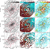Fig. 11.

Ionised gas moment maps. Left columns: Intensity map in grey-scale from faint (grey) to bright (black) of the Hα, [NII] and [OIII] lines (from top to bottom). The contour levels for the intensity map are given in the colour bar at the top. The red contours refer to the radio continuum (levels: 0.08, 0.31, 0.80, 1.68 mJy beam⁻¹). Central columns: Peak-velocity field with respect to the systemic velocity (1456.4 km s⁻¹). The dashed contours refer to the approaching side, while the solid lines correspond to receding velocities. The radio continuum is overlaid with orange contours. Right panels: Velocity dispersion map of the aforementioned lines. The contour levels are given in the colour bar. The black contours refer to the radio continuum. In all the top panels the 1 kpc reference scale is shown at the top left.

The presence of non-rotating gas is also evident from the channel maps in a 800 km s⁻¹ range around Hα, provided in Fig. A.8. This velocity range is sufficient to cover the emission from Hα and prevent significant contamination from the wings of the [NII] doublet, as indicated by the dispersion map in the right panels of Fig. 11. The maps further corroborate the spatial coincidence between Hα and the bright radio continuum tracing the inner regions of the jets. This suggests that within 1.5 kpc from the centre the jet is impacting ISM, affecting its kinematics and physical state.

The output of the nGIST pipeline includes the stellar kinematics map obtained from the fit to the stellar absorption lines. We use the map to derive the rotation curve of the stellar disc. This has been computed with the 2DFIT task of 3D-Barolo. We fitted the rotation velocity and position angle of 100 rings, each 0.3″ wide. We fixed the inclination of the rings to 46°, i.e. the optical inclination of the galaxy as listed in de Blok et al. (2024), the radial velocities to 0 km s⁻¹, and the systemic velocity also to 0 km s⁻¹, as the kinematics map is already corrected for it. We use this information to compare with the ionised gas kinematics. The 7″-wide pv diagram extracted along the major axis, given in Fig. 12, shows this comparison. The identification of the aforementioned kinematically anomalous gas, indicated by the arrows in Fig. 12, suggests again that probably a jet-induced outflow is present in the nuclear region.

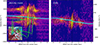Fig. 12.

Position-velocity diagrams of the ionised gas. The left panel shows the pv diagram along the major axis (θ = 135°) of the [NII]-Hα triplet, whereas the right panel shows the pv diagram of the [OIII] line. The contours denote the (2, 4, 8, 16, 21)σ level. The dashed black horizontal line corresponds to the Hα and [OIII] systemic velocity. The cyan line corresponds to the stellar rotation curve. The inset shows the velocity field of Hα, overlaid with the radio continuum (pink contours) and the slice from which the pv is extracted (black hatched area). The arrows indicate kinematically anomalous features.

To further explore the jet-ISM interaction in NGC 1371 we investigated the impact of the radio jet on the molecular gas. This phenomenon has been well studied with CO observations (e.g. Alatalo et al. 2011; Cicone et al. 2014; Morganti et al. 2015, 2021; Oosterloo et al. 2017, 2019; Fluetsch et al. 2019; Ruffa et al. 2020, 2022; Maccagni et al. 2021; Audibert et al. 2023). We visually inspected the low-resolution ACA cube (beam: Ω = 14″ × 14″; channel separation: Δv = 4.4 km s⁻¹) presented in Sect. 2.3 resulting in no detection. Searching for emission with SoFiA-2 also provides no reliable sources at the 3σ level. After converting the brightness temperature noise value (σ_{T_b} = 3 mK) into Jy (Meyer et al. 2017)

$\begin{matrix} \frac{σ_{S}}{Jy} = 4.8 \times 10^{12} \frac{k_{b} ν_{obs}^{2} Ω σ_{T_{b}}}{c^{2}}, \end{matrix}$ $\begin{aligned} \frac{\sigma _{\rm S}}{\mathrm{Jy}} = 4.8\times 10^{12}\frac{k_{\rm b}\nu _{\mathrm{obs}}^2\Omega \sigma _{T_{\rm b}}}{c^2}, \end{aligned}$ (5)

where k_b is the Boltzmann constant, Ω is the beam area in arcsec², and 4.8 × 10¹² accounts for the steradians-to-arcsec² and Jy-to-erg s⁻¹ conversions, we calculated an upper limit on the molecular mass (M_H₂) using

$\begin{matrix} M_{H_{2}} = L_{CO} \cdot α_{CO}, \end{matrix}$ $\begin{aligned} M_{\mathrm{H}_{2}}=L_{\rm CO}\cdot \alpha _{\rm CO}, \end{aligned}$ (6)

where α_CO = 4.36 M_⊙ is a standard CO-to-H₂ conversion factor (Tacconi et al. 2013; Bolatto et al. 2013; Audibert et al. 2022, 2023) and

$\begin{matrix} \frac{L_{CO}}{{K km s}^{- 1} {pc}^{- 2}} = 3.25 \times 10^{7} (\frac{σ_{S}}{Jy}) (\frac{Δ v}{{km s}^{- 1}}) {(\frac{D_{L}}{Mpc})}^{2} {(\frac{ν_{obs}}{Hz})}^{- 2} \end{matrix}$ $\begin{aligned} \frac{L_{\rm CO}}{\mathrm{K\,km\,s}^{-1}\,\mathrm{pc}^{-2}} = 3.25\times 10^7\left(\frac{\sigma _{\rm S}}{\mathrm{Jy}}\right)\left(\frac{\Delta v}{\mathrm{km\,s}^{-1}}\right)\left(\frac{D_{\rm L}}{\mathrm{Mpc}}\right)^2\left(\frac{\nu _{\rm obs}}{\mathrm{Hz}}\right)^{-2} \end{aligned}$ (7)

is the CO luminosity (Solomon & Vanden Bout 2005). The estimated upper limit in the inner 5 kpc of the galaxy (i.e. within the H I hole) is $M_{H_{2}}^{hole} < 2 \times 10^{5} M_{⊙}$ $M^{\mathrm{hole}}_{\mathrm{H}_{2}} < 2\times10^5\,\mathrm{M}_{\odot}$ . This value is three orders of magnitude lower than the typical molecular mass detected in circumnuclear disks of AGNs (e.g. Maccagni et al. 2018; Ruffa et al. 2019; Combes et al. 2019) and about two dex lower if we compare with the upper limits for non-detected disks (Tadhunter et al. 2024). This may indicate a lack of molecular gas or that it is just warmer (T ∼ tens of K, Oosterloo et al. 2017). In the latter scenario, the CO_2 → 1 or CO_3 → 2 emission lines are much brighter than CO_1 → 0 (e.g. Alatalo et al. 2011; Oosterloo et al. 2017, 2019; Ruffa et al. 2022). Observations using these lines would clarify the lack of detectable CO_1 → 0.

In conclusion, we found indications that in the inner 3 kpc of NGC 1371 the low-power jet is producing an outflow in the ionised phase of the gas. We found no detectable CO_1 → 0 down to 2 × 10⁵ M_⊙ within the inner 5 kpc, where also H I is not detected up to column densities of 1.1 × 10¹⁹ cm⁻². It is not clear why only the hot phase of the gas survives in the central region.

4.6. The absence of cold ISM

Jet-ISM coupling typically does not prevent the cooling of the gas and the survivability of neutral and molecular hydrogen. Evidence is the large amount of H I (e.g. Morganti et al. 2003, 2016; Morganti & Oosterloo 2018; Gupta et al. 2006; Chandola et al. 2011; Mahony et al. 2013; Geréb et al. 2015; Maccagni et al. 2017) and CO (e.g. Alatalo et al. 2011; Cicone et al. 2014; Morganti et al. 2015, 2021; Oosterloo et al. 2017, 2019; Fluetsch et al. 2019; Ruffa et al. 2020, 2022; Maccagni et al. 2021; Audibert et al. 2023) observations of such interactions, as well as the support from theoretical works (e.g. Mukherjee et al. 2018a,b; Tanner & Weaver 2022). Also, the effect of the jet is directional, while in NGC 1371 the non-detection of cold gas is ubiquitous. However, since the gas in the galaxy rotates, one possible way out is that in the inner 5 kpc of NGC 1371 the gas cooling time is higher than its orbital time. Assuming the gas corotates with the stellar disk on circular orbits, from the stellar rotation curve derived earlier we calculate the orbital period. This ranges from ∼10 to ∼70 Myr, which implies cooling times of similar amplitudes. This is not an unreasonable range, given the many physical parameters affecting the cooling of the gas, such as its density, metallicity, and temperature (e.g. Valentini & Brighenti 2015; Kanjilal et al. 2021; Dutta et al. 2024).

Another possibility is that the gas is blown out by a wind. Based on observations of 94 AGNs with detected sub-parsec to kiloparsec winds, Fiore et al. (2017) argued that AGN winds are very efficient in removing cold gas from the nuclear region of galaxies. At L_bol ∼ 10⁴⁵ erg s⁻¹ the wind reaches velocities of ∼700 km s⁻¹ and the molecular mass outflow is ∼200 M_⊙ yr⁻¹, while at L_bol ∼ 10⁴² erg s⁻¹ the wind speed is ∼200 km s⁻¹ and the outflow reaches ∼1 M_⊙ yr⁻¹. We recall that the estimated bolometric luminosity for NGC 1371 is L_bol ∼ 10⁴² erg s⁻¹ (Cisternas et al. 2013), implying wind speeds of ∼200 km s⁻¹ and an outflow rate of ∼1 M_⊙ yr⁻¹. This is reasonable for NGC 1371, as the velocity dispersion of the ionised gas, which could be used to trace also the molecular wind speed (Fiore et al. 2017), is ∼200 km s⁻¹ along the radio jet (see the top right panel of Fig. 11).

Another process capable of removing gas from the central region of galaxies is bar quenching (Khoperskov et al. 2018; George et al. 2019). Stellar bars are commonly found in the inner regions of disk galaxies (e.g. Menéndez-Delmestre et al. 2007; Hernández-Toledo et al. 2007; Marinova & Jogee 2007 and for our Galaxy Binney et al. 1991; Blitz & Spergel 1991; Weiland et al. 1994) and there is growing observational (Masters et al. 2010; Cheung et al. 2013; Gavazzi et al. 2015; James & Percival 2016; Kim et al. 2017; Wang et al. 2020; Scaloni et al. 2024) and theoretical (e.g. Carles et al. 2016; Spinoso et al. 2017) evidence, even in our Galaxy (Haywood et al. 2016, 2018), that bars favour the rapid depletion of gas and the inside-out quenching of disk galaxies. Based on near-infrared imaging with the Infrared Array Camera (IRAC; Fazio et al. 2004), Cisternas et al. (2013) classified NGC 1371 as a barred galaxy (see also Kim et al. 2015). Therefore, it is plausible that in this galaxy the lack of cold ISM in the inner 5 kpc results from the rapid depletion of gas from the bar.

Ultimately, we found that the low-power, inclined jet propagating in an under-dense ISM could explain the inside-out quenching of NGC 1371, although the stellar bar might play a significant role as well. Future hydrodynamical simulations of tilted jets and future observations of a sample of galaxies sharing similar properties (stellar bar, H I hole, low-power tilted jet) should be able to favour one of the possible scenario we proposed to explain the lack of cold gas in the inner 5 kpc: the ISM is not cold but warm, hence should be traced via CO_2 → 1 or CO_3 → 2 emission lines; the ISM has been mostly blown out by the AGN wind or it has been depleted by the stellar bar.

4.7. Star formation in the H I disc

Having established the dual relevance of the stellar bar and the low-luminosity AGN in perturbing the gas in the inner 5 kpc of the galaxy, we want to understand how far out in the gaseous disk the influence of these two processes extends. This requires studying whether the SFR is consistent with the gaseous content of the disk. The relation between the gas density of the ISM and the SFR is given by the Kennicutt-Schmidt law (Schmidt 1959; Kennicutt 1998; Kennicutt & Evans 2012; de los Reyes & Kennicutt 2019). This relation is well known and very tight for the molecular phase of the gas (e.g. Bigiel et al. 2008; Marasco et al. 2012; Leroy et al. 2013; de los Reyes & Kennicutt 2019), yet the precise correlation between Σ_SFR and the H I surface density (Σ_H I) remains a matter of debate (e.g. Kennicutt et al. 2007; Leroy et al. 2008; Bigiel et al. 2010; Roychowdhury et al. 2015; Yim & van der Hulst 2016; Bacchini et al. 2019; Eibensteiner et al. 2024).

The computation of the Σ_SFR maps is provided in Sect. 3.2. We derived Σ_H I from the inclination and primary beam-corrected moment 0 map (I_H I). First, we converted I_H I into column density (N_H I; Meyer et al. 2017),

$\begin{matrix} \frac{N_{H i}}{{atoms cm}^{- 2}} = 1.25 \times 10^{24} (\frac{I_{H i}}{{Jy km s}^{- 1}}) {(\frac{Ω}{{arcsec}^{2}})}^{- 1}, \end{matrix}$ $\begin{aligned} \frac{N_{\mathrm{H}\,{i }}}{\mathrm{atoms~cm}^{-2}} = 1.25\times 10^{24}\left(\frac{I_{\mathrm{H}\,{i }}}{\mathrm{Jy\,km\,s}^{-1}}\right)\left(\frac{\Omega }{\mathrm{arcsec}^2}\right)^{-1} ,\end{aligned}$ (8)

where Ω is the beam area. Then, we computed Σ_H I using

$\begin{matrix} \frac{Σ_{H i}}{M_{⊙} {pc}^{- 2}} = 7.95 \times 10^{- 19} (\frac{N_{H i}}{{atoms cm}^{- 2}}), \end{matrix}$ $\begin{aligned} \frac{\Sigma _{{\mathrm{H}\,{i }}}}{\mathrm{M}_\odot \,\mathrm{pc}^{-2}} = 7.95\times 10^{-19}\left(\frac{N_{{\mathrm{H}\,{i }}}}{\mathrm{atoms~cm}^{-2}}\right) ,\end{aligned}$ (9)

where 7.95 × 10⁻¹⁹ accounts for the centimetre-to-parsec and atoms-to-M_⊙ conversions. In the left panel of Fig. 13 we show the spatially resolved Σ_SFR as a function of Σ_H I. We also plot the relations found by Roychowdhury et al. (2015) for H I-dominated regions in spiral galaxies from the THINGS (Walter et al. 2008), the Bluedisk (Wang et al. 2013) and a control sample. The majority of the points are consistent with these relations, thus, most of the H I disk follows the expected Kennicutt-Schmidt law.

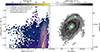Fig. 13.

Spatially resolved Kennicutt-Schimdt law. Left panel: Density plot of Σ_SFR as a function of Σ_H I. The two-dimensional histogram is made of 49 × 49 hexagonal bins, each containing at least 1 pixel. The coloured lines indicate the relations found by Roychowdhury et al. (2015) for H I dominated regions in spiral galaxies; the solid and dashed black curves refer to the relation found for THINGS (Walter et al. 2008) galaxies studied at 0.4 kpc resolution (solid line) and 1 kpc resolution (dashed line); the dotted cyan line indicates the relation found for the Bluedisk sample (Wang et al. 2013); the dash-dotted line refers to the control sample used by Roychowdhury et al. (2015). The silver-hatched area indicates the ±5σ scatter of the relation relative to the THINGS galaxies at 0.4 kpc resolution. Bins with magenta edges correspond to pixels within the dashed magenta elliptical annulus in the right panel. Right panel: Σ_H I map. The contour levels are given in the colour bar. The green regions indicate the location of the pixel which are in the hatched area in the left panel. The dashed magenta elliptical annulus provides the approximate location of a star-forming ring observed outside the H I hole.

In the right panel of Fig. 13, we instead plot Σ_H I overlaid with the locations of the pixels within the hatched area. Examining their spatial distribution, we found that most of the outliers are located around the H I hole. The reason for their displacement from the Kennicutt-Schmidt law is possibly that in this region of the disk Σ_H I is decreasing towards the center, whereas Σ_SFR is not, as shown in Fig. A.9. One explanation could be that the H I is turning molecular. H I holes in the centres of spiral galaxies are known to result from the conversion of H I into H₂ (Leroy et al. 2008; Bigiel et al. 2008). However, based on the very low upper limit on the molecular mass, derived at the beginning of this section (M_H₂ < 5 × 10⁶ M_⊙), we think this is unlikely. It is more probable that Σ_H I is decreasing due to the dual effect of the low-power AGN and the bar quenching, as explained in Sect. 4.5 and in Sect. 4.6.

From the multi-wavelength image in Fig. 1 and the SFR map of Fig. 8 it is evident a ring of star formation just outside the H I hole. In the right panel of Fig. 13 we show its approximate location with the dashed magenta elliptical annulus. The spatially resolved KS law for the pixels in the annulus is reported in left panel of Fig. 13 with the bins having magenta edges. These bins are mostly concentrated around the relations for H I-dominated regions, meaning they follow the KS law. Therefore, the star-forming ring may indicates the radii at which the inside-out quenching stops, and the gas is forming stars as expected in H I dominated regions.

In conclusion, we found that up to ∼10 kpc from the centre, the gas might still be affected by the processes that are removing or heating the ISM within the H I hole, i.e. AGN winds and/or the stellar bar. At larger radii, however, the disk is forming stars as expected from the Kennicutt-Schmidt relation of H I-dominated regions in spiral galaxies. Yet, the inner quenching of star formation appears enough to prevent the formation of the ∼1.75 M_⊙ yr⁻¹ needed to bring the galaxy back on the star-forming main sequence.

4.8. The impact of the environment

So far we have considered only the internal processes affecting the star formation and the state of the gas in NGC 1371. It is known that also external processes tidal interaction and gas stripping are able to impact the star formation of galaxies from both theoretical (Hirschmann et al. 2014; Hatfield & Jarvis 2017) predictions and empirical (Peng et al. 2015; Knobel et al. 2015) evidence. As mentioned in Sect. 1, NGC 1371 is a member of the Eridanus group (Brough et al. 2006), therefore it is worth investigating if there is any environmental effect acting on this galaxy. In Sect. 2.1 we already excluded a possible recent or ongoing interaction between NGC 1371 and the newly-discovered companion MKT 033442-245148. The H I disk is also not showing strong tidal features, like filaments and tails, but it is warped in the outermost regions. Thus, it can still be that the H I disk of NGC 1371 is being perturbed by the presence of the nearby companions.

The Eridanus group comprises at least 35 galaxies (For et al. 2023). Using WALLABY pre-pilot data, For et al. (2023) studied the H I properties of this group, finding that all the galaxies show a distorted H I morphology. They suggests that group interactions are occurring. The most massive neighbour of NGC 1371 is NGC 1385 (Log M_* = 10.13, Log M_H I = 9.34; For et al. 2023). Its distance (D) from NGC 1371 can be roughly estimated using

$\begin{matrix} \frac{D}{Mpc} = \sqrt{{(\frac{dl}{Mpc})}^{2} + {(\frac{d α}{Mpc})}^{2} + {(\frac{d δ}{Mpc})}^{2}}, \end{matrix}$ $\begin{aligned} \frac{D}{\mathrm{Mpc}}=\sqrt{\left(\frac{dl}{\mathrm{Mpc}}\right)^2+\left(\frac{d\alpha }{\mathrm{Mpc}}\right)^2+\left(\frac{d\delta }{\mathrm{Mpc}}\right)^2} ,\end{aligned}$ (10)

where dD, dα, and dδ are the distance and the projected right ascension and declination difference, respectively. Using the distance provided by (Leroy et al. 2019) and the fiducial position reported in NED for NGC 1385, we estimate D ∼ 0.3 Mpc. This distance is lower than the AMIGA isolation radius¹¹ (Verdes-Montenegro et al. 2005) of ∼0.9 Mpc, assuming an H I-based diameter for NGC 1385 and NGC 1371 of ∼46 kpc and ∼84 kpc, respectively, and lower than the NGC 1371 virial radius R₂₀₀ ∼ 0.37 Mpc (de Blok et al. 2024). From the above considerations, it is plausible that a weak interaction is ongoing between NGC 1371 and NGC 1385, but evident signatures of gas removal are not found. Therefore, we argue that the environment plays a minor role in the quenching of NGC 1371.

5. Conclusions and future prospects

In this paper we presented the deepest 21 cm spectral line and 1.4 GHz continuum observation ever taken of the nearby spiral galaxy NGC 1371. This galaxy is below the star-forming main sequence; our aim was to understand why that is. In the following we list our main findings:

(i)
The radio continuum reveals a low-luminosity ( $L_{1.4 GHz}^{jet} = (9.75 \pm 0.04) \times 10^{20}$ $L^{\mathrm{jet}}_{1.4\,\mathrm{GHz}}=(9.75\pm0.04)\times10^{20}$ W Hz⁻¹) jet extending up to 5 kpc (in projection) from the galactic centre.
(ii)
In the radio continuum we also detected ∼10 kpc wide bipolar nuclear bubbles, having total luminosity of $L_{1.4 GHz}^{bubbles} < 4.6 \times 10^{20}$ $L^{\mathrm{bubbles}}_{1.4\,\mathrm{GHz}} < 4.6\times10^{20}$ W Hz⁻¹. Such structures have never been observed before in NGC 1371 and are rarely seen in other galaxies.
(iii)
We do not find compelling evidence that the bubbles in NGC 1371 are an extragalactic analogue of our Galaxy FEBs, and yet we cannot exclude that they are the same class of object.
(iv)
The presence of such bubbles and their S-shaped limb brightening suggests that the jet in NGC 1371 is likely emitted with an angle > 45° with respect to the galaxy rotational axis.
(v)
There are indications that the tilted jet is producing an ionised gas outflow in the innermost kiloparsec (in projection).
(vi)
The H I is mostly distributed in a regularly rotating disk and peculiar features includes a warped outer disk and a ∼5 kpc wide H I hole around the galactic centre.
(vii)
Within the H I hole the molecular gas traced by the CO_1 → 0 transition was not detected, which allowed us to compute only an upper limit (M_H₂ < 2 × 10⁵ M_⊙).
(viii)
The lack of cold gas can be explained if the ISM affected by the AGN is warm, if its cooling time is longer than its orbital time (< 70 Myr), or if it has been blown out by AGN winds or depleted by the stellar bar. We argue that one (or more) of these four scenarios is causing the inside-out quenching of NGC 1371.
(ix)
At larger distances, the gaseous disk is forming stars, as expected from the Kennicutt-Schmidt relation of H I-dominated regions in spiral galaxies.
(x)
In the galaxy environment, we identified a new galaxy. MKT 033442-245148 (α = 3^h34^m42.31^s, δ = −24^d51^m47.52^s, cz = 1647 km s⁻¹) has a H I mass of M_H I = 6.6 × 10⁶ M_⊙ and we did not find strong evidence for a recent interaction with NGC 1371. Instead, from the isolation radius of NGC 1371 we found that the galaxy is probably weakly interacting with the neighbour NGC 1385, although we do not have enough elements to quantify the impact on its quenching.

Some aspects are still unclear. In the future, deriving the star formation history of NGC 1371 and the age of its bubbles is fundamental in order to understand if the bubbles could be the remnant of a past star burst in the stellar bar. Observing the NGC 1371 centre with higher excitation lines of CO (CO_2 → 1 and CO_3 → 2) would be useful to confirm if our CO_1 → 0 non-detection is due to the lack of molecular gas or to a higher medium temperature. It would also be useful to further investigate 3D hydrodynamical simulations of a low-power jet (P_jet < 10⁴¹ erg s⁻¹) propagating at an angle > 45° with respect to the galaxy rotational axis within a medium pre-processed by a stellar bar or an AGN wind. This will provide insights into why in NGC 1371 we are not detecting the neutral and molecular ISM in the inner 5 kpc of this galaxy. Moreover, these simulations will allow the inside-quenching to be studied in this peculiarenvironment.

¹

The MeerKAT telescope is operated by the South African Radio Astronomy Observatory, which is a facility of the National Research Foundation, an agency of the Department of Science and Innovation.

²

The velocity field colour map look-up table throughout this paper is taken from English et al. (2024).

³

The pv are 1 beam wide and were extracted with the pvextractor package (https://pvextractor.readthedocs.io/en/latest/).

⁴

The NASA/IPAC Extragalactic Database (NED) is funded by the National Aeronautics and Space Administration and operated by the California Institute of Technology.

⁵

The north-west emission is a background AGN.

⁶

We ran the task with its default input arguments, except for thresh_isl, which was set to 2.5.

⁷

The fit is performed with the curve_fit task of SciPy (Virtanen et al. 2020), which performs a non-linear least squares fit to the data.

⁸

http://ascl.net/1907.025

⁹

We tested different combinations of lower- and higher-degree polynomials and we found that this combination provides the best fit.

¹⁰

The velocity dispersion has been corrected for the instrumental broadening: $σ_{0} = \sqrt{σ^{2} - σ_{ins}^{2}}$ $\sigma_0=\sqrt{\sigma^2-\sigma^2_{\mathrm{ins}}}$ .

¹¹

The isolation radius for a galaxy of diameter d₀ with respect to a neighbour having diameter 0.25d₀ < d₁ < 4d₀ is equal to 20d₁.

Acknowledgments

We thank the anonymous referee for the constructive comments. This work has received funding from the European Research Council (ERC) under the European Union’s Horizon 2020 research and innovation programme (grant agreement No 882793 ‘MeerGas’). FMM acknowledges that (part of) the research activities described in this paper were carried out with contribution of the Next Generation EU funds within the National Recovery and Resilience Plan (PNRR), Mission 4 – Education and Research, Component 2 – From Research to Business (M4C2), Investment Line 3.1 – Strengthening and creation of Research Infrastructures, Project IR0000034 – “STILES – Strengthening the Italian Leadership in ELT and SKA. This research has made use of the NASA/IPAC Extragalactic Database (NED), which is funded by the National Aeronautics and Space Administration and operated by the California Institute of Technology. This paper makes use of the following ALMA data: ADS/JAO.ALMA#2022.1.01314.S. ALMA is a partnership of ESO (representing its member states), NSF (USA) and NINS (Japan), together with NRC (Canada), NSTC and ASIAA (Taiwan), and KASI (Republic of Korea), in cooperation with the Republic of Chile. The Joint ALMA Observatory is operated by ESO, AUI/NRAO and NAOJ. SV thanks E. di Teodoro for the insightful discussions about kinematical modelling of galaxy disks.

References

Abbott, T. M. C., Adamów, M., Aguena, M., et al. 2021, ApJS, 255, 20 [NASA ADS] [CrossRef] [Google Scholar]
Abdo, A. A., Ackermann, M., Ajello, M., et al. 2009, ApJ, 707, L142 [NASA ADS] [CrossRef] [Google Scholar]
Alatalo, K., Blitz, L., Young, L. M., et al. 2011, ApJ, 735, 88 [NASA ADS] [CrossRef] [Google Scholar]
Alatalo, K., Appleton, P. N., Lisenfeld, U., et al. 2014, ApJ, 795, 159 [Google Scholar]
An, F., Vaccari, M., Smail, I., et al. 2021, MNRAS, 507, 2643 [NASA ADS] [CrossRef] [Google Scholar]
An, F., Vaccari, M., Best, P. N., et al. 2024, MNRAS, 528, 5346 [NASA ADS] [CrossRef] [Google Scholar]
Audibert, A., Dasyra, K. M., Papachristou, M., et al. 2022, A&A, 668, A67 [NASA ADS] [CrossRef] [EDP Sciences] [Google Scholar]
Audibert, A., Ramos Almeida, C., García-Burillo, S., et al. 2023, A&A, 671, L12 [NASA ADS] [CrossRef] [EDP Sciences] [Google Scholar]
Bacchini, C., Fraternali, F., Iorio, G., & Pezzulli, G. 2019, A&A, 622, A64 [NASA ADS] [CrossRef] [EDP Sciences] [Google Scholar]
Bacon, R., Accardo, M., Adjali, L., et al. 2010, SPIE Conf. Ser., 7735 [Google Scholar]
Bagchi, J., Vivek, M., Vikram, V., et al. 2014, ApJ, 788, 174 [NASA ADS] [CrossRef] [Google Scholar]
Baldwin, J. A., Phillips, M. M., & Terlevich, R. 1981, PASP, 93, 5 [Google Scholar]
Baum, S. A., O’Dea, C. P., Dallacassa, D., de Bruyn, A. G., & Pedlar, A. 1993, ApJ, 419, 553 [NASA ADS] [CrossRef] [Google Scholar]
Begeman, K. G. 1987, Ph.D. Thesis, Kapteyn Institute [Google Scholar]
Bigiel, F., Leroy, A., Walter, F., et al. 2008, AJ, 136, 2846 [NASA ADS] [CrossRef] [Google Scholar]
Bigiel, F., Leroy, A., Walter, F., et al. 2010, AJ, 140, 1194 [NASA ADS] [CrossRef] [Google Scholar]
Binney, J., Gerhard, O. E., Stark, A. A., Bally, J., & Uchida, K. I. 1991, MNRAS, 252, 210 [Google Scholar]
Bittner, A., Falcón-Barroso, J., Nedelchev, B., et al. 2019, A&A, 628, A117 [NASA ADS] [CrossRef] [EDP Sciences] [Google Scholar]
Bland-Hawthorn, J., Maloney, P. R., Sutherland, R., et al. 2019, ApJ, 886, 45 [Google Scholar]
Blitz, L., & Spergel, D. N. 1991, ApJ, 379, 631 [Google Scholar]
Bluck, A. F. L., Maiolino, R., Brownson, S., et al. 2022, A&A, 659, A160 [NASA ADS] [CrossRef] [EDP Sciences] [Google Scholar]
Blundell, K. M., & Rawlings, S. 2000, AJ, 119, 1111 [NASA ADS] [CrossRef] [Google Scholar]
Bolatto, A. D., Wolfire, M., & Leroy, A. K. 2013, ARA&A, 51, 207 [CrossRef] [Google Scholar]
Bouquin, A. Y. K., Gil de Paz, A., Muñoz-Mateos, J. C., et al. 2018, ApJS, 234, 18 [NASA ADS] [CrossRef] [Google Scholar]
Bower, R. G., Benson, A. J., Malbon, R., et al. 2006, MNRAS, 370, 645 [Google Scholar]
Braun, R., & Thilker, D. A. 2004, A&A, 417, 421 [NASA ADS] [CrossRef] [EDP Sciences] [Google Scholar]
Brough, S., Forbes, D. A., Kilborn, V. A., Couch, W., & Colless, M. 2006, MNRAS, 369, 1351 [NASA ADS] [CrossRef] [Google Scholar]
Butler, A., Huynh, M., Kapińska, A., et al. 2019, A&A, 625, A111 [NASA ADS] [CrossRef] [EDP Sciences] [Google Scholar]
Cappellari, M. 2009, arXiv e-prints [arXiv:0912.1303] [Google Scholar]
Cappellari, M. 2017, MNRAS, 466, 798 [Google Scholar]
Cappellari, M. 2023, MNRAS, 526, 3273 [NASA ADS] [CrossRef] [Google Scholar]
Cappellari, M., & Copin, Y. 2003, MNRAS, 342, 345 [Google Scholar]
Cappellari, M., & Emsellem, E. 2004, PASP, 116, 138 [Google Scholar]
Carles, C., Martel, H., Ellison, S. L., & Kawata, D. 2016, MNRAS, 463, 1074 [NASA ADS] [CrossRef] [Google Scholar]
Cavagnolo, K. W., McNamara, B. R., Nulsen, P. E. J., et al. 2010, ApJ, 720, 1066 [Google Scholar]
Cecil, G., Greenhill, L. J., DePree, C. G., et al. 2000, ApJ, 536, 675 [Google Scholar]
Chandola, Y., Sirothia, S. K., & Saikia, D. J. 2011, MNRAS, 418, 1787 [NASA ADS] [CrossRef] [Google Scholar]
Chen, Q., Meyer, M., Popping, A., et al. 2021, MNRAS, 508, 2758 [NASA ADS] [CrossRef] [Google Scholar]
Cheung, E., Athanassoula, E., Masters, K. L., et al. 2013, ApJ, 779, 162 [NASA ADS] [CrossRef] [Google Scholar]
Cicone, C., Maiolino, R., Sturm, E., et al. 2014, A&A, 562, A21 [NASA ADS] [CrossRef] [EDP Sciences] [Google Scholar]
Ciotti, L., Ostriker, J. P., & Proga, D. 2010, ApJ, 717, 708 [Google Scholar]
Cisternas, M., Gadotti, D. A., Knapen, J. H., et al. 2013, ApJ, 776, 50 [NASA ADS] [CrossRef] [Google Scholar]
Clark, P. C., Glover, S. C. O., Klessen, R. S., & Bonnell, I. A. 2012, MNRAS, 424, 2599 [CrossRef] [Google Scholar]
Cluver, M. E., Jarrett, T. H., Dale, D. A., et al. 2025, ApJ, 979, 18 [Google Scholar]
Combes, F., García-Burillo, S., Audibert, A., et al. 2019, A&A, 623, A79 [NASA ADS] [CrossRef] [EDP Sciences] [Google Scholar]
Cook, R. H. W., Davies, L. J. M., Rhee, J., et al. 2024, MNRAS, 531, 708 [Google Scholar]
Cresci, G., Mainieri, V., Brusa, M., et al. 2015a, ApJ, 799, 82 [Google Scholar]
Cresci, G., Marconi, A., Zibetti, S., et al. 2015b, A&A, 582, A63 [NASA ADS] [CrossRef] [EDP Sciences] [Google Scholar]
Crocker, R. M., & Aharonian, F. 2011, Phys. Rev. Lett., 106, 101102 [Google Scholar]
Crocker, R. M., Bicknell, G. V., Taylor, A. M., & Carretti, E. 2015, ApJ, 808, 107 [NASA ADS] [CrossRef] [Google Scholar]
Croton, D. J. 2006, MNRAS, 369, 1808 [NASA ADS] [CrossRef] [Google Scholar]
Daly, R. A., Sprinkle, T. B., O’Dea, C. P., Kharb, P., & Baum, S. A. 2012, MNRAS, 423, 2498 [NASA ADS] [CrossRef] [Google Scholar]
Danovich, M., Dekel, A., Hahn, O., Ceverino, D., & Primack, J. 2015, MNRAS, 449, 2087 [Google Scholar]
Dark Energy Survey Collaboration (Abbott, T., et al.) 2016, MNRAS, 460, 1270 [Google Scholar]
Das, S., Sardone, A., Leroy, A. K., et al. 2020, ApJ, 898, 15 [NASA ADS] [CrossRef] [Google Scholar]
Das, S., Rickel, M., Leroy, A., et al. 2024, MNRAS, 527, 10358 [Google Scholar]
Davé, R., Finlator, K., & Oppenheimer, B. D. 2012, MNRAS, 421, 98 [Google Scholar]
Davé, R., Rafieferantsoa, M. H., Thompson, R. J., & Hopkins, P. F. 2017, MNRAS, 467, 115 [NASA ADS] [Google Scholar]
Davé, R., Anglés-Alcázar, D., Narayanan, D., et al. 2019, MNRAS, 486, 2827 [Google Scholar]
Davis, B. L., Berrier, J. C., Johns, L., et al. 2014, ApJ, 789, 124 [NASA ADS] [CrossRef] [Google Scholar]
de Blok, W. J. G., Healy, J., Maccagni, F. M., et al. 2024, A&A, 688, A109 [NASA ADS] [CrossRef] [EDP Sciences] [Google Scholar]
de Gasperin, F., Orrú, E., Murgia, M., et al. 2012, A&A, 547, A56 [NASA ADS] [CrossRef] [EDP Sciences] [Google Scholar]
de los Reyes, M. A. C., & Kennicutt, R. C., Jr. 2019, ApJ, 872, 16 [NASA ADS] [CrossRef] [Google Scholar]
Dekel, A., & Birnboim, Y. 2006, MNRAS, 368, 2 [NASA ADS] [CrossRef] [Google Scholar]
Dekel, A., Birnboim, Y., Engel, G., et al. 2009, Nature, 457, 451 [Google Scholar]
Dey, A., Schlegel, D. J., Lang, D., et al. 2019, AJ, 157, 168 [Google Scholar]
Di Matteo, T., Springel, V., & Hernquist, L. 2005, Nature, 433, 604 [NASA ADS] [CrossRef] [Google Scholar]
Di Teodoro, E. M., & Fraternali, F. 2015, MNRAS, 451, 3021 [Google Scholar]
Di Teodoro, E. M., & Peek, J. E. G. 2021, ApJ, 923, 220 [NASA ADS] [CrossRef] [Google Scholar]
Dickinson, C. 2018, Galaxies, 6, 56 [NASA ADS] [CrossRef] [Google Scholar]
Doi, A., Nagira, H., Kawakatu, N., et al. 2012, ApJ, 760, 41 [NASA ADS] [CrossRef] [Google Scholar]
Dubois, Y., Peirani, S., Pichon, C., et al. 2016, MNRAS, 463, 3948 [Google Scholar]
Dutta, R., Sharma, P., Sarkar, K. C., & Stone, J. M. 2024, ApJ, 973, 148 [CrossRef] [Google Scholar]
Eckart, A., Witzel, A., Biermann, P., et al. 1986, A&A, 168, 17 [NASA ADS] [Google Scholar]
Egorov, O. V., Lozinskaya, T. A., Moiseev, A. V., & Shchekinov, Y. A. 2017, MNRAS, 464, 1833 [NASA ADS] [CrossRef] [Google Scholar]
Egorov, O. V., Kreckel, K., Glover, S. C. O., et al. 2023, A&A, 678, A153 [NASA ADS] [CrossRef] [EDP Sciences] [Google Scholar]
Eibensteiner, C., Sun, J., Bigiel, F., et al. 2024, A&A, 691, A163 [NASA ADS] [CrossRef] [EDP Sciences] [Google Scholar]
Emsellem, E., Schinnerer, E., Santoro, F., et al. 2022, A&A, 659, A191 [NASA ADS] [CrossRef] [EDP Sciences] [Google Scholar]
English, J., Richardson, M. L. A., Ferrand, G., & Deg, N. 2024, Astrophysics Source Code Library [record ascl:2401.005] [Google Scholar]
Evans, I. N., Primini, F. A., Glotfelty, K. J., et al. 2010, ApJS, 189, 37 [NASA ADS] [CrossRef] [Google Scholar]
Event Horizon Telescope Collaboration (Akiyama, K., et al.) 2022a, ApJ, 930, L15 [NASA ADS] [CrossRef] [Google Scholar]
Event Horizon Telescope Collaboration (Akiyama, K., et al.) 2022b, ApJ, 930, L12 [NASA ADS] [CrossRef] [Google Scholar]
Fabian, A. C. 2012, ARA&A, 50, 455 [Google Scholar]
Faucher-Giguère, C.-A., & Oh, S. P. 2023, ARA&A, 61, 131 [CrossRef] [Google Scholar]
Fazio, G. G., Hora, J. L., Allen, L. E., et al. 2004, ApJS, 154, 10 [Google Scholar]
Fielding, D. B., & Bryan, G. L. 2022, ApJ, 924, 82 [NASA ADS] [CrossRef] [Google Scholar]
Fiore, F., Feruglio, C., Shankar, F., et al. 2017, A&A, 601, A143 [NASA ADS] [CrossRef] [EDP Sciences] [Google Scholar]
Fluetsch, A., Maiolino, R., Carniani, S., et al. 2019, MNRAS, 483, 4586 [NASA ADS] [Google Scholar]
For, B. Q., Spekkens, K., Staveley-Smith, L., et al. 2023, MNRAS, 526, 3130 [NASA ADS] [CrossRef] [Google Scholar]
Fraser-McKelvie, A., van de Sande, J., Gadotti, D. A., et al. 2025a, A&A, 700, A237 [NASA ADS] [CrossRef] [EDP Sciences] [Google Scholar]
Fraser-McKelvie, A., van de Sande, J., Brown, T., et al. 2025b, Astrophysics Source Code Library [record ascl:2507.015] [Google Scholar]
Fraternali, F. 2017, Astrophys. Space Sci. Lib., 430, 323 [CrossRef] [Google Scholar]
Fraternali, F., & Binney, J. J. 2006, MNRAS, 366, 449 [CrossRef] [Google Scholar]
Fraternali, F., & Tomassetti, M. 2012, MNRAS, 426, 2166 [NASA ADS] [CrossRef] [Google Scholar]
Gallagher, R., Maiolino, R., Belfiore, F., et al. 2019, MNRAS, 485, 3409 [NASA ADS] [CrossRef] [Google Scholar]
Gaspari, M., McDonald, M., Hamer, S. L., et al. 2018, ApJ, 854, 167 [Google Scholar]
Gavazzi, G., Consolandi, G., Dotti, M., et al. 2015, A&A, 580, A116 [NASA ADS] [CrossRef] [EDP Sciences] [Google Scholar]
George, K., Subramanian, S., & Paul, K. T. 2019, A&A, 628, A24 [NASA ADS] [CrossRef] [EDP Sciences] [Google Scholar]
Geréb, K., Maccagni, F. M., Morganti, R., & Oosterloo, T. A. 2015, A&A, 575, A44 [CrossRef] [EDP Sciences] [Google Scholar]
Gillessen, S., Eisenhauer, F., Trippe, S., et al. 2009, ApJ, 692, 1075 [NASA ADS] [CrossRef] [Google Scholar]
Grundy, J. A., Wong, O. I., Lee-Waddell, K., et al. 2023, PASA, 40, e012 [Google Scholar]
Gupta, N., Salter, C. J., Saikia, D. J., Ghosh, T., & Jeyakumar, S. 2006, MNRAS, 373, 972 [NASA ADS] [CrossRef] [Google Scholar]
Hameed, S., & Devereux, N. 1999, AJ, 118, 730 [Google Scholar]
Hardcastle, M. J., Evans, D. A., & Croston, J. H. 2007, MNRAS, 376, 1849 [NASA ADS] [CrossRef] [Google Scholar]
Harrison, C. M., Thomson, A. P., Alexander, D. M., et al. 2015, ApJ, 800, 45 [Google Scholar]
Harrison, C. M., Costa, T., Tadhunter, C. N., et al. 2018, Nat. Astron., 2, 198 [Google Scholar]
Harwood, J. J., Hardcastle, M. J., Croston, J. H., & Goodger, J. L. 2013, MNRAS, 435, 3353 [NASA ADS] [CrossRef] [Google Scholar]
Haslam, C. G. T., Salter, C. J., Stoffel, H., & Wilson, W. E. 1982, A&AS, 47, 1 [NASA ADS] [Google Scholar]
Hatfield, P. W., & Jarvis, M. J. 2017, MNRAS, 472, 3570 [Google Scholar]
Hayward, C. C., & Hopkins, P. F. 2017, MNRAS, 465, 1682 [Google Scholar]
Haywood, M., Lehnert, M. D., Di Matteo, P., et al. 2016, A&A, 589, A66 [NASA ADS] [CrossRef] [EDP Sciences] [Google Scholar]
Haywood, M., Di Matteo, P., Lehnert, M., et al. 2018, A&A, 618, A78 [NASA ADS] [CrossRef] [EDP Sciences] [Google Scholar]
Heckman, T. M. 1980, A&A, 87, 152 [Google Scholar]
Heckman, T. M., & Best, P. N. 2014, ARA&A, 52, 589 [Google Scholar]
Heckman, T. M., & Best, P. N. 2023, Galaxies, 11, 21 [NASA ADS] [CrossRef] [Google Scholar]
Heckman, T. M., Roy, N., Best, P. N., & Kondapally, R. 2024, ApJ, 977, 125 [Google Scholar]
Hernández-Toledo, H. M., Zendejas-Domínguez, J., & Avila-Reese, V. 2007, AJ, 134, 2286 [Google Scholar]
Heywood, I. 2020, Astrophysics Source Code Library [record ascl:2009.003] [Google Scholar]
Hirschmann, M., De Lucia, G., Wilman, D., et al. 2014, MNRAS, 444, 2938 [NASA ADS] [CrossRef] [Google Scholar]
Ho, L. C., Feigelson, E. D., Townsley, L. K., et al. 2001, ApJ, 549, L51 [NASA ADS] [CrossRef] [Google Scholar]
Hota, A., & Saikia, D. J. 2006, MNRAS, 371, 945 [NASA ADS] [CrossRef] [Google Scholar]
Hughes, J. P., Chugai, N., Chevalier, R., Lundqvist, P., & Schlegel, E. 2007, ApJ, 670, 1260 [Google Scholar]
Ianjamasimanana, R., de Blok, W. J. G., Walter, F., & Heald, G. H. 2012, AJ, 144, 96 [NASA ADS] [CrossRef] [Google Scholar]
Iguchi, S., Morita, K.-I., Sugimoto, M., et al. 2009, PASJ, 61, 1 [NASA ADS] [CrossRef] [Google Scholar]
Ishibashi, W., & Fabian, A. C. 2012, MNRAS, 427, 2998 [NASA ADS] [CrossRef] [Google Scholar]
James, P. A., & Percival, S. M. 2016, MNRAS, 457, 917 [Google Scholar]
Jonas, J.& MeerKAT Team. 2016, in MeerKAT Science: On the Pathway to the SKA, 1 [Google Scholar]
Józsa, G. I. G., White, S. V., Thorat, K., et al. 2020, Astrophysics Source Code Library [record ascl:2006.014] [Google Scholar]
Kalberla, P. M. W., Burton, W. B., Hartmann, D., et al. 2005, A&A, 440, 775 [NASA ADS] [CrossRef] [EDP Sciences] [Google Scholar]
Kamphuis, P., Jütte, E., Heald, G. H., et al. 2022, A&A, 668, A182 [NASA ADS] [CrossRef] [EDP Sciences] [Google Scholar]
Kanjilal, V., Dutta, A., & Sharma, P. 2021, MNRAS, 501, 1143 [Google Scholar]
Kataoka, J., Tahara, M., Totani, T., et al. 2013, ApJ, 779, 57 [NASA ADS] [CrossRef] [Google Scholar]
Kataoka, J., Sofue, Y., Inoue, Y., et al. 2018, Galaxies, 6, 27 [Google Scholar]
Kauffmann, G., Heckman, T. M., Tremonti, C., et al. 2003, MNRAS, 346, 1055 [Google Scholar]
Kennicutt, R. C., Jr. 1998, ApJ, 498, 541 [Google Scholar]
Kennicutt, R. C., & Evans, N. J. 2012, ARA&A, 50, 531 [NASA ADS] [CrossRef] [Google Scholar]
Kennicutt, R. C., Jr., Calzetti, D., Walter, F., et al. 2007, ApJ, 671, 333 [Google Scholar]
Kereš, D., Katz, N., Weinberg, D. H., & Davé, R. 2005, MNRAS, 363, 2 [Google Scholar]
Kereš, D., Katz, N., Fardal, M., Davé, R., & Weinberg, D. H. 2009, MNRAS, 395, 160 [Google Scholar]
Kewley, L. J., Dopita, M. A., Sutherland, R. S., Heisler, C. A., & Trevena, J. 2001, ApJ, 556, 121 [Google Scholar]
Kewley, L. J., Groves, B., Kauffmann, G., & Heckman, T. 2006, MNRAS, 372, 961 [Google Scholar]
Khandai, N., Di Matteo, T., Croft, R., et al. 2015, MNRAS, 450, 1349 [NASA ADS] [CrossRef] [Google Scholar]
Khoperskov, S., Haywood, M., Di Matteo, P., Lehnert, M. D., & Combes, F. 2018, A&A, 609, A60 [NASA ADS] [CrossRef] [EDP Sciences] [Google Scholar]
Kim, M., & Oh, S.-H. 2022, J. Korean Astron. Soc., 55, 149 [Google Scholar]
Kim, T., Sheth, K., Gadotti, D. A., et al. 2015, ApJ, 799, 99 [NASA ADS] [CrossRef] [Google Scholar]
Kim, E., Hwang, H. S., Chung, H., et al. 2017, ApJ, 845, 93 [CrossRef] [Google Scholar]
Klein, U., Lisenfeld, U., & Verley, S. 2018, A&A, 611, A55 [NASA ADS] [CrossRef] [EDP Sciences] [Google Scholar]
Knobel, C., Lilly, S. J., Woo, J., & Kovač, K. 2015, ApJ, 800, 24 [NASA ADS] [CrossRef] [Google Scholar]
Kondapally, R., Best, P. N., Raouf, M., et al. 2023, MNRAS, 523, 5292 [NASA ADS] [CrossRef] [Google Scholar]
Koribalski, B. S., Staveley-Smith, L., Westmeier, T., et al. 2020, Ap&SS, 365, 118 [Google Scholar]
Krause, M., Fendt, C., & Neininger, N. 2007, A&A, 467, 1037 [NASA ADS] [CrossRef] [EDP Sciences] [Google Scholar]
Krumholz, M. R., McKee, C. F., & Tumlinson, J. 2009, ApJ, 699, 850 [NASA ADS] [CrossRef] [Google Scholar]
Ledlow, M. J., Owen, F. N., & Keel, W. C. 1998, ApJ, 495, 227 [Google Scholar]
Leroy, A. K., Walter, F., Brinks, E., et al. 2008, AJ, 136, 2782 [Google Scholar]
Leroy, A. K., Walter, F., Sandstrom, K., et al. 2013, AJ, 146, 19 [Google Scholar]
Leroy, A. K., Sandstrom, K. M., Lang, D., et al. 2019, ApJS, 244, 24 [Google Scholar]
Li, A., Marasco, A., Fraternali, F., Trager, S., & Verheijen, M. A. W. 2021, MNRAS, 504, 3013 [NASA ADS] [CrossRef] [Google Scholar]
Li, J.-T., Wang, Q. D., Wiegert, T., et al. 2022, MNRAS, 515, 2483 [Google Scholar]
Lilly, S. J., Carollo, C. M., Pipino, A., Renzini, A., & Peng, Y. 2013, ApJ, 772, 119 [NASA ADS] [CrossRef] [Google Scholar]
Liu, Y., Zhu, M., Yu, H., et al. 2023, MNRAS, 523, 3905 [NASA ADS] [CrossRef] [Google Scholar]
Maccagni, F. M., Morganti, R., Oosterloo, T. A., Geréb, K., & Maddox, N. 2017, A&A, 604, A43 [NASA ADS] [CrossRef] [EDP Sciences] [Google Scholar]
Maccagni, F. M., Morganti, R., Oosterloo, T. A., Oonk, J. B. R., & Emonts, B. H. C. 2018, A&A, 614, A42 [NASA ADS] [CrossRef] [EDP Sciences] [Google Scholar]
Maccagni, F. M., Serra, P., Gaspari, M., et al. 2021, A&A, 656, A45 [NASA ADS] [CrossRef] [EDP Sciences] [Google Scholar]
Madau, P., & Dickinson, M. 2014, ARA&A, 52, 415 [Google Scholar]
Magnelli, B., Ivison, R. J., Lutz, D., et al. 2015, A&A, 573, A45 [NASA ADS] [CrossRef] [EDP Sciences] [Google Scholar]
Mahony, E. K., Morganti, R., Emonts, B. H. C., Oosterloo, T. A., & Tadhunter, C. 2013, MNRAS, 435, L58 [NASA ADS] [CrossRef] [Google Scholar]
Mahony, E. K., Oonk, J. B. R., Morganti, R., et al. 2016, MNRAS, 455, 2453 [NASA ADS] [CrossRef] [Google Scholar]
Mancera Piña, P. E., Fraternali, F., Oosterloo, T., et al. 2022, MNRAS, 512, 3230 [CrossRef] [Google Scholar]
Mancera Piña, P. E., Golini, G., Trujillo, I., & Montes, M. 2024, A&A, 689, A344 [NASA ADS] [CrossRef] [EDP Sciences] [Google Scholar]
Marasco, A., Fraternali, F., & Binney, J. J. 2012, MNRAS, 419, 1107 [NASA ADS] [CrossRef] [Google Scholar]
Marasco, A., Cresci, G., Nardini, E., et al. 2020, A&A, 644, A15 [EDP Sciences] [Google Scholar]
Marasco, A., Fraternali, F., Lehner, N., & Howk, J. C. 2022, MNRAS, 515, 4176 [NASA ADS] [CrossRef] [Google Scholar]
Marinacci, F., Binney, J., Fraternali, F., et al. 2010, MNRAS, 404, 1464 [NASA ADS] [Google Scholar]
Marinacci, F., Fraternali, F., Nipoti, C., et al. 2011, MNRAS, 415, 1534 [CrossRef] [Google Scholar]
Marinova, I., & Jogee, S. 2007, ApJ, 659, 1176 [Google Scholar]
Martin, D. C., Fanson, J., Schiminovich, D., et al. 2005, ApJ, 619, L1 [Google Scholar]
Masters, K. L., Mosleh, M., Romer, A. K., et al. 2010, MNRAS, 405, 783 [NASA ADS] [Google Scholar]
McCarthy, I. G., Schaye, J., Bird, S., & Le Brun, A. M. C. 2017, MNRAS, 465, 2936 [Google Scholar]
McCourt, M., Sharma, P., Quataert, E., & Parrish, I. J. 2012, MNRAS, 419, 3319 [NASA ADS] [CrossRef] [Google Scholar]
Meidt, S. E., Hughes, A., Dobbs, C. L., et al. 2015, ApJ, 806, 72 [NASA ADS] [CrossRef] [Google Scholar]
Meliani, Z., Cristofari, P., Rodríguez-González, A., et al. 2024, A&A, 683, A178 [NASA ADS] [CrossRef] [EDP Sciences] [Google Scholar]
Menéndez-Delmestre, K., Sheth, K., Schinnerer, E., Jarrett, T. H., & Scoville, N. Z. 2007, ApJ, 657, 790 [Google Scholar]
Meyer, M., Robotham, A., Obreschkow, D., et al. 2017, PASA, 34, 52 [Google Scholar]
Miller, M. J., & Bregman, J. N. 2016, ApJ, 829, 9 [NASA ADS] [CrossRef] [Google Scholar]
Mohan, N., & Rafferty, D. 2015, Astrophysics Source Code Library [record ascl:1502.007] [Google Scholar]
Mondal, S., Keshet, U., Sarkar, K. C., & Gurwich, I. 2022, MNRAS, 514, 2581 [NASA ADS] [CrossRef] [Google Scholar]
Morganti, R., & Oosterloo, T. 2018, A&ARv, 26, 4 [Google Scholar]
Morganti, R., Oosterloo, T., & Tsvetanov, Z. 1998, AJ, 115, 915 [NASA ADS] [CrossRef] [Google Scholar]
Morganti, R., Oosterloo, T. A., Emonts, B. H. C., van der Hulst, J. M., & Tadhunter, C. N. 2003, ApJ, 593, L69 [NASA ADS] [CrossRef] [Google Scholar]
Morganti, R., Holt, J., Tadhunter, C., et al. 2011, A&A, 535, A97 [NASA ADS] [CrossRef] [EDP Sciences] [Google Scholar]
Morganti, R., Oosterloo, T., Oonk, J. B. R., Frieswijk, W., & Tadhunter, C. 2015, A&A, 580, A1 [NASA ADS] [CrossRef] [EDP Sciences] [Google Scholar]
Morganti, R., Veilleux, S., Oosterloo, T., Teng, S. H., & Rupke, D. 2016, A&A, 593, A30 [NASA ADS] [CrossRef] [EDP Sciences] [Google Scholar]
Morganti, R., Oosterloo, T., Tadhunter, C., Bernhard, E. P., & Raymond Oonk, J. B. 2021, A&A, 656, A55 [NASA ADS] [CrossRef] [EDP Sciences] [Google Scholar]
Mou, G., Yuan, F., Bu, D., Sun, M., & Su, M. 2014, ApJ, 790, 109 [NASA ADS] [CrossRef] [Google Scholar]
Mou, G., Yuan, F., Gan, Z., & Sun, M. 2015, ApJ, 811, 37 [Google Scholar]
Mukherjee, D., Bicknell, G. V., Wagner, A. Y., Sutherland, R. S., & Silk, J. 2018a, MNRAS, 479, 5544 [NASA ADS] [CrossRef] [Google Scholar]
Mukherjee, D., Wagner, A. Y., Bicknell, G. V., et al. 2018b, MNRAS, 476, 80 [NASA ADS] [CrossRef] [Google Scholar]
Nelson, D., Genel, S., Pillepich, A., et al. 2016, MNRAS, 460, 2881 [NASA ADS] [CrossRef] [Google Scholar]
Nelson, D., Pillepich, A., Springel, V., et al. 2018, MNRAS, 475, 624 [Google Scholar]
Offringa, A. R., & Smirnov, O. 2017, MNRAS, 471, 301 [Google Scholar]
Offringa, A. R., McKinley, B., Hurley-Walker, N., et al. 2014, MNRAS, 444, 606 [Google Scholar]
Omar, A., & Dwarakanath, K. S. 2005, JApA, 26, 89 [NASA ADS] [Google Scholar]
Oosterloo, T., Raymond Oonk, J. B., Morganti, R., et al. 2017, A&A, 608, A38 [NASA ADS] [CrossRef] [EDP Sciences] [Google Scholar]
Oosterloo, T., Morganti, R., Tadhunter, C., et al. 2019, A&A, 632, A66 [NASA ADS] [CrossRef] [EDP Sciences] [Google Scholar]
Ostriker, E. C., McKee, C. F., & Leroy, A. K. 2010, ApJ, 721, 975 [CrossRef] [Google Scholar]
Owen, F. N., Eilek, J. A., & Kassim, N. E. 2000, ApJ, 543, 611 [NASA ADS] [CrossRef] [Google Scholar]
Peng, Y.-J., & Maiolino, R. 2014, MNRAS, 443, 3643 [NASA ADS] [CrossRef] [Google Scholar]
Peng, Y., Maiolino, R., & Cochrane, R. 2015, Nature, 521, 192 [Google Scholar]
Péroux, C., & Howk, J. C. 2020, ARA&A, 58, 363 [CrossRef] [Google Scholar]
Planck Collaboration XXV. 2016, A&A, 594, A25 [NASA ADS] [CrossRef] [EDP Sciences] [Google Scholar]
Ponti, G., Hofmann, F., Churazov, E., et al. 2019, Nature, 567, 347 [Google Scholar]
Pontzen, A., Tremmel, M., Roth, N., et al. 2017, MNRAS, 465, 547 [Google Scholar]
Pracy, M. B., Ching, J. H. Y., Sadler, E. M., et al. 2016, MNRAS, 460, 2 [Google Scholar]
Putman, M. E., Peek, J. E. G., & Joung, M. R. 2012, ARA&A, 50, 491 [Google Scholar]
Ressler, S. M., White, C. J., & Quataert, E. 2023, MNRAS, 521, 4277 [CrossRef] [Google Scholar]
Roychowdhury, S., Huang, M.-L., Kauffmann, G., Wang, J., & Chengalur, J. N. 2015, MNRAS, 449, 3700 [NASA ADS] [CrossRef] [Google Scholar]
Ruffa, I., Prandoni, I., Laing, R. A., et al. 2019, MNRAS, 484, 4239 [NASA ADS] [CrossRef] [Google Scholar]
Ruffa, I., Laing, R. A., Prandoni, I., et al. 2020, MNRAS, 499, 5719 [NASA ADS] [CrossRef] [Google Scholar]
Ruffa, I., Prandoni, I., Davis, T. A., et al. 2022, MNRAS, 510, 4485 [NASA ADS] [CrossRef] [Google Scholar]
Saintonge, A., & Catinella, B. 2022, ARA&A, 60, 319 [NASA ADS] [CrossRef] [Google Scholar]
Saintonge, A., Lutz, D., Genzel, R., et al. 2013, ApJ, 778, 2 [Google Scholar]
Saintonge, A., Catinella, B., Cortese, L., et al. 2016, MNRAS, 462, 1749 [Google Scholar]
Samal, M. R., Zavagno, A., Deharveng, L., et al. 2014, A&A, 566, A122 [NASA ADS] [CrossRef] [EDP Sciences] [Google Scholar]
Santoro, F., Oonk, J. B. R., Morganti, R., & Oosterloo, T. 2015a, A&A, 574, A89 [NASA ADS] [CrossRef] [EDP Sciences] [Google Scholar]
Santoro, F., Oonk, J. B. R., Morganti, R., Oosterloo, T. A., & Tremblay, G. 2015b, A&A, 575, L4 [NASA ADS] [CrossRef] [EDP Sciences] [Google Scholar]
Sarkar, K. C. 2019, MNRAS, 482, 4813 [NASA ADS] [CrossRef] [Google Scholar]
Sarkar, K. C. 2024, A&ARv, 32, 1 [NASA ADS] [CrossRef] [Google Scholar]
Scaloni, L., Rodighiero, G., Enia, A., et al. 2024, A&A, 687, A255 [NASA ADS] [CrossRef] [EDP Sciences] [Google Scholar]
Schaye, J. 2004, ApJ, 609, 667 [NASA ADS] [CrossRef] [Google Scholar]
Schaye, J., Crain, R. A., Bower, R. G., et al. 2015, MNRAS, 446, 521 [Google Scholar]
Schinnerer, E., Hughes, A., Leroy, A., et al. 2019, ApJ, 887, 49 [NASA ADS] [CrossRef] [Google Scholar]
Schmidt, M. 1959, ApJ, 129, 243 [NASA ADS] [CrossRef] [Google Scholar]
Schneider, E. E., Robertson, B. E., & Thompson, T. A. 2018, ApJ, 862, 56 [NASA ADS] [CrossRef] [Google Scholar]
Schneider, E. E., Ostriker, E. C., Robertson, B. E., & Thompson, T. A. 2020, ApJ, 895, 43 [NASA ADS] [CrossRef] [Google Scholar]
Sharma, P., Quataert, E., & Stone, J. M. 2007, ApJ, 671, 1696 [Google Scholar]
Sharma, P., McCourt, M., Quataert, E., & Parrish, I. J. 2012, MNRAS, 420, 3174 [NASA ADS] [CrossRef] [Google Scholar]
Silk, J. 2013, ApJ, 772, 112 [Google Scholar]
Silk, J., & Mamon, G. A. 2012, Res. Astron. Astrophys., 12, 917 [Google Scholar]
Singh, V., Ishwara-Chandra, C. H., Sievers, J., et al. 2015, MNRAS, 454, 1556 [NASA ADS] [CrossRef] [Google Scholar]
Solomon, P. M., & Vanden Bout, P. A. 2005, ARA&A, 43, 677 [NASA ADS] [CrossRef] [Google Scholar]
Somerville, R. S., & Davé, R. 2015, ARA&A, 53, 51 [Google Scholar]
Spinoso, D., Bonoli, S., Dotti, M., et al. 2017, MNRAS, 465, 3729 [NASA ADS] [CrossRef] [Google Scholar]
Springel, V., Di Matteo, T., & Hernquist, L. 2005, MNRAS, 361, 776 [Google Scholar]
Stilp, A. M., Dalcanton, J. J., Warren, S. R., et al. 2013, ApJ, 765, 136 [NASA ADS] [CrossRef] [Google Scholar]
Su, M., Slatyer, T. R., & Finkbeiner, D. P. 2010, ApJ, 724, 1044 [Google Scholar]
Swarup, G. 1990, Indian J. Radio Space Phys., 19, 493 [NASA ADS] [Google Scholar]
Tabatabaei, F. S., Schinnerer, E., Krause, M., et al. 2017, ApJ, 836, 185 [Google Scholar]
Tabatabaei, F. S., Minguez, P., Prieto, M. A., & Fernández-Ontiveros, J. A. 2018, Nat. Astron., 2, 83 [Google Scholar]
Tacconi, L. J., Neri, R., Genzel, R., et al. 2013, ApJ, 768, 74 [NASA ADS] [CrossRef] [Google Scholar]
Tacconi, L. J., Genzel, R., & Sternberg, A. 2020, ARA&A, 58, 157 [NASA ADS] [CrossRef] [Google Scholar]
Tadhunter, C., Oosterloo, T., Morganti, R., et al. 2024, MNRAS, 532, 4463 [Google Scholar]
Tamburro, D., Rix, H. W., Leroy, A. K., et al. 2009, AJ, 137, 4424 [Google Scholar]
Tamhane, P. D., McNamara, B. R., Russell, H. R., et al. 2023, MNRAS, 519, 3338 [NASA ADS] [CrossRef] [Google Scholar]
Tanner, R., & Weaver, K. A. 2022, AJ, 163, 134 [NASA ADS] [CrossRef] [Google Scholar]
Thomas, N., Davé, R., Jarvis, M. J., & Anglés-Alcázar, D. 2021, MNRAS, 503, 3492 [NASA ADS] [CrossRef] [Google Scholar]
Thompson, T. A., & Heckman, T. M. 2024, ARA&A, 62, 529 [NASA ADS] [CrossRef] [Google Scholar]
Thompson, T. A., Quataert, E., Zhang, D., & Weinberg, D. H. 2016, MNRAS, 455, 1830 [CrossRef] [Google Scholar]
Tumlinson, J., Peeples, M. S., & Werk, J. K. 2017, ARA&A, 55, 389 [Google Scholar]
Ulvestad, J. S., Wrobel, J. M., & Carilli, C. L. 1999, ApJ, 516, 127 [NASA ADS] [CrossRef] [Google Scholar]
Ursino, E., Galeazzi, M., & Liu, W. 2016, ApJ, 816, 33 [Google Scholar]
Valentini, M., & Brighenti, F. 2015, MNRAS, 448, 1979 [NASA ADS] [CrossRef] [Google Scholar]
van de Voort, F., Schaye, J., Booth, C. M., Haas, M. R., & Dalla Vecchia, C. 2011, MNRAS, 414, 2458 [NASA ADS] [CrossRef] [Google Scholar]
Vazdekis, A., Koleva, M., Ricciardelli, E., Röck, B., & Falcón-Barroso, J. 2016, MNRAS, 463, 3409 [Google Scholar]
Venturi, G., Cresci, G., Marconi, A., et al. 2021, A&A, 648, A17 [NASA ADS] [CrossRef] [EDP Sciences] [Google Scholar]
Venturi, G., Treister, E., Finlez, C., et al. 2023, A&A, 678, A127 [NASA ADS] [CrossRef] [EDP Sciences] [Google Scholar]
Verdes-Montenegro, L., Sulentic, J., Lisenfeld, U., et al. 2005, A&A, 436, 443 [NASA ADS] [CrossRef] [EDP Sciences] [Google Scholar]
Vidal, M., Dickinson, C., Davies, R. D., & Leahy, J. P. 2015, MNRAS, 452, 656 [NASA ADS] [CrossRef] [Google Scholar]
Virtanen, P., Gommers, R., Oliphant, T. E., et al. 2020, Nat. Methods, 17, 261 [Google Scholar]
Wagner, A. Y., Bicknell, G. V., & Umemura, M. 2012, ApJ, 757, 136 [CrossRef] [Google Scholar]
Walch, S., Girichidis, P., Naab, T., et al. 2015, MNRAS, 454, 238 [Google Scholar]
Walter, F., Brinks, E., de Blok, W. J. G., et al. 2008, AJ, 136, 2563 [Google Scholar]
Walter, F., Carilli, C., Neeleman, M., et al. 2020, ApJ, 902, 111 [Google Scholar]
Wang, J., Kauffmann, G., Józsa, G. I. G., et al. 2013, MNRAS, 433, 270 [Google Scholar]
Wang, J., Athanassoula, E., Yu, S.-Y., et al. 2020, ApJ, 893, 19 [NASA ADS] [CrossRef] [Google Scholar]
Weiland, J. L., Arendt, R. G., Berriman, G. B., et al. 1994, ApJ, 425, L81 [NASA ADS] [CrossRef] [Google Scholar]
Weisskopf, M. C., Tananbaum, H. D., Van Speybroeck, L. P., & O’Dell, S. L. 2000, SPIE Conf. Ser., 4012, 2 [Google Scholar]
Wenger, M., Ochsenbein, F., Egret, D., et al. 2000, A&AS, 143, 9 [NASA ADS] [CrossRef] [EDP Sciences] [Google Scholar]
Westmeier, T., Kitaeff, S., Pallot, D., et al. 2021, MNRAS, 506, 3962 [NASA ADS] [CrossRef] [Google Scholar]
Willott, C. J., Rawlings, S., Blundell, K. M., & Lacy, M. 1999, MNRAS, 309, 1017 [Google Scholar]
Wilson, A. S., Yang, Y., & Cecil, G. 2001, ApJ, 560, 689 [NASA ADS] [CrossRef] [Google Scholar]
Wolfe, S. A., Pisano, D. J., Lockman, F. J., McGaugh, S. S., & Shaya, E. J. 2013, Nature, 497, 224 [NASA ADS] [CrossRef] [Google Scholar]
Wolfe, S. A., Lockman, F. J., & Pisano, D. J. 2016, ApJ, 816, 81 [NASA ADS] [CrossRef] [Google Scholar]
Woo, J.-H., Schulze, A., Park, D., et al. 2013, ApJ, 772, 49 [NASA ADS] [CrossRef] [Google Scholar]
Wright, E. L., Eisenhardt, P. R. M., Mainzer, A. K., et al. 2010, AJ, 140, 1868 [Google Scholar]
Xu, C. K., Cheng, C., Appleton, P. N., et al. 2022, Nature, 610, 461 [NASA ADS] [CrossRef] [Google Scholar]
Yang, Q., Wu, X.-B., Fan, X., et al. 2018, ApJ, 862, 109 [Google Scholar]
Yang, H. Y. K., Ruszkowski, M., & Zweibel, E. G. 2022, Nat. Astron., 6, 584 [NASA ADS] [CrossRef] [Google Scholar]
Yim, K., & van der Hulst, J. M. 2016, MNRAS, 463, 2092 [Google Scholar]
Yu, S., Bullock, J. S., Wetzel, A., et al. 2020, MNRAS, 494, 1539 [Google Scholar]
Yun, M. S., Reddy, N. A., & Condon, J. J. 2001, ApJ, 554, 803 [Google Scholar]
Zajaček, M., Busch, G., Valencia-S., M., et al. 2019, A&A, 630, A83 [Google Scholar]
Zeng, Y., Wang, Q. D., & Fraternali, F. 2023, MNRAS, 526, 483 [NASA ADS] [CrossRef] [Google Scholar]
Zhang, R., & Guo, F. 2020, ApJ, 894, 117 [Google Scholar]
Zhuang, M.-Y., & Ho, L. C. 2020, ApJ, 896, 108 [NASA ADS] [CrossRef] [Google Scholar]
Zinger, E., Pillepich, A., Nelson, D., et al. 2020, MNRAS, 499, 768 [CrossRef] [Google Scholar]
Zinn, P. C., Middelberg, E., Norris, R. P., & Dettmar, R. J. 2013, ApJ, 774, 66 [NASA ADS] [CrossRef] [Google Scholar]

Appendix A: Ancillary plots

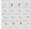Fig. A.1.

NGC 1371 H I channel maps from 1250 km s⁻¹ to 1665 km s⁻¹ in steps of 28 km s⁻¹. The coloured contours correspond to column densities of (4.3, 8.6, 17.3, 34.5) × 10¹⁸ cm⁻², equivalent to (4, 8, 16, 32)σ. The dashed grey contours denote the column density of −4.3 × 10¹⁸ cm⁻². At the bottom, we report the LoS velocity (with respect to the systemic velocity) in each channel and at the top left the 10 kpc reference scale. In the bottom right corner the 13.7″×9.6″ beam is displayed.

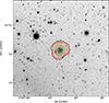Fig. A.2.

Combined gzri DECaLS image of MKT 033442-245148 overlaid with the H I contours denoting the (0.1, 0.6, 2.2, 5.8, 12.1)×10¹⁹ cm⁻² column density levels.

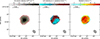Fig. A.3.

High-resolution H I moment maps of MKT 033442-245148. Left panel: Primary beam-corrected H I column-density map. Central panel: Intensity-weighted mean velocity field with respect to the systemic velocity (1647 km s⁻¹). The dashed contours refer to the approaching side, while the solid lines correspond to receding velocities. Right panel: moment 2 map. In all panels the contour levels are given on the colour bar, while in the bottom right corner we show the 13.7″×9.6″ beam and in the top left corner the 3 kpc reference scale.

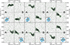Fig. A.4.

Low-resolution position-velocity diagrams at azimuthal angles (θ) of (0, 30, 60, 90, 120, 150) for the data and the best-fit model derived by 3D-Barolo fitting the approaching and receding side of the galaxy simultaneously. Both the data and the model cube were Hanning-smoothed at 7 km s⁻¹. For each panel, the background grey-scale image is the slice extracted from the data cube. Solid contour levels are denoting the (4, 16, 64, 256, 1024)σ. The coloured lines refer to the model, the green curves to the data. The dashed grey contours refers to the −4σ level. The dashed black horizontal line corresponds to the systemic velocity, while the dash-dotted black vertical line denotes the 0-offset. The insets shows the moment 2 map and the slice along which the pv is extracted. The letters A and B provide the orientation in the main panels.

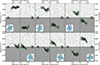Fig. A.5.

Same as in Fig. A.4, but for the fit on the receding side only. The shaded area indicates the approaching side.

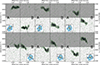Fig. A.6.

Same as in Fig. A.4, but for the fit on the approaching side only. The shaded area indicates the receding side.

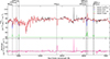Fig. A.7.

4750-7100Å integrated spectrum of the inner 5 kpc. The observed spectrum is reported in black, while the best-fit stellar continuum and the emission lines from the ionised gas are shown in blue and green, respectively. The model, i.e. the sum of the blue and green curves, is plotted in red. We shifted the emission lines flux up by 50 × 10⁻¹⁵ erg s⁻¹ cm⁻² for visualisation purposes. The bottom panel contains the residuals in terms of data−model. The observed 5775-6010Å range was originally masked because it is affected by the adaptive optics laser. The flux in these channels is set to the median value of the spectrum prior the fit. The high residual spikes around 6300Å are not real emission lines, but faulty channels.

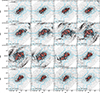Fig. A.8.

NGC 1371 Hα channel maps from −455 km s⁻¹ to 398 km s⁻¹ from the Hα systemic velocity in steps of 57 km s⁻¹. The colour-scale contours correspond to flux densities of (18, 36, 73, 146) × 10^-20 ergs s⁻¹ cm⁻² Å⁻¹, equivalent to (4, 8, 16, 32)σ. The dashed grey contours denote the −4σ level. At the bottom, we report the LoS velocity (with respect to the Hα systemic velocity) in each channel and at the top left the 2.5 kpc reference scale. The blue contours in all panels indicates the radio continuum (levels: 0.08, 0.31, 0.80, 1.68 mJy beam⁻¹)

Fig. A.9.

Radial profile of Σ_SFR (red) and Σ_H I (blue). The coloured shaded area is the standard deviation. The vertical magenta dashed lines indicate the approximate location of the star-forming ring. The left y-axis refers to Σ_H I, the right y-axis to Σ_SFR.

All Tables

Table 1.

NGC 1371 main observational properties.

NGC 1371 radio flux.

Comparison of Sgr A^⋆ and the SMBH in NGC 1371.

In the text

All Figures

	Fig. 1. Multi-wavelength image of NGC 1371. The background shows the combined gzri optical image from Dark Energy Camera Legacy Survey (DECaLS, Dey et al. 2019). The MeerKAT high-resolution 1.4 GHz radio continuum is shown in yellow and red. The UV emission as observed by GALEX is overlaid in pink. The multi-resolution H I from the MHOONGOOSE observations is given in green and blue.
In the text

Fig. 2.

High-resolution H I moment maps of NGC 1371. Left panel: Primary beam-corrected H I column-density map. The contour levels are given on the colour bar. In the bottom right we show the 13.7″ × 9.6″ beam. The 10 kpc reference scale is shown in the top left. Central panel: Intensity-weighted mean velocity field with respect to the systemic velocity (1456.4 km s⁻¹). The dashed contours refer to the approaching side, while the solid lines correspond to receding velocities. Right panel: moment 2 map, i.e. the velocity spread along each LoS. It corresponds to the velocity dispersion when the emission comes from a single line or to the spread of multiple components at different velocities.

In the text

Fig. 3.

Position-velocity diagrams at azimuthal angles (θ) of (0, 30, 60, 90, 120, 150) degrees with respect to the major axis in the plane of the sky. The data cube was spectrally smoothed with a 7 km s⁻¹ Hanning kernel. The solid contour levels denote the (4, 16, 64, 256, 1024)σ level, where σ = 0.03 mJy beam⁻¹. The dashed grey contours refers to the −4σ level. The dashed black horizontal line corresponds to the systemic velocity, while the dash-dotted black vertical line denotes the centre of the galaxy. The insets shows the moment 2 map and the slice along which the pv is extracted. The letters A and B provide the orientation in the main panels.

In the text

Fig. 4.

Comparison of the best-fit parameters for the 3D model derived by 3D-Barolo fitting the approaching and receding side of the galaxy separately and simultaneously. From left to right and from top to bottom each panel shows v_rot, σ₀, v_rad, Σ_H I, i, and PA. The pink points refer to the best fit on the receding side, blue to the approaching side, and green to the simultaneous fit. The black horizontal dashed line in the v_rad panel is a visual guide indicating the 0-level, whereas in the i panel is the indicative optical inclination angle from NED (de Blok et al. 2024).

In the text

	Fig. 5. Comparison between the observed (left) and mock (right) moment-2 map derived with `3D-Barolo`. In the bottom right corner the 13.7″ × 9.6″ beam is displayed.
In the text

Fig. 6.

1.4 GHz continuum maps. From left to right: Observed radio continuum, best-fit model from pPyBDSF, and the residuals in terms of data-model. The contour levels, with the lowest corresponding to 3σ, are given by the colour bar at the top. A 5 kpc reference line is given in the bottom left corner. In the central panel we indicate with blue arrows the locations of the core (C), the two inner hotspots (I), and the two outer hotspots (O). In the right panel we highlight the edge-brightening of the bubbles with the cyan dashed contours, corresponding to a flux density of 10 μJy beam⁻¹.

In the text

Fig. 7.

Spatially resolved 950–1408 MHz spectral index map (left panel) and percentage uncertainty (right panel). The white regions in the left panel are due to the masking of contaminant sources and unreliable fits (see text for the details). The contour levels are given in the colour bar. In the right panel we show the percentage error on the spectral index in terms of $100 \cdot \frac{Δ α}{α}$ $100\cdot\frac{\Delta\alpha}{\alpha}$ , where Δα is the uncertainty on α as derived by the least-squares fit. The LoS where Δα > 50% are marked in red. These were removed from the map on the left. Contaminant sources are masked. In both maps, the black contours refers to the radio continuum from the jet (levels: 36, 141, 367, 772 μJy beam⁻¹), while the 7.4″ × 6.7″ beam is reported in the bottom right corner and a 5 kpc reference line is given in the top left corner.

In the text

	Fig. 8. Star formation density map derived with the prescription given in Leroy et al. (2019). The black contours correspond to H I column densities of (0.3, 2.9, 11.3, 29.5, 62.1) × 10¹⁹ cm^-2.
In the text

	Fig. 9. Overlays of the H I (left), star formation density (center), and optical (right) map with the radio continuum contours. Contour levels are (0.006, 0.06, 0.2, 0.6, 1.3) mJy beam⁻¹, with the lowest being equivalent to 5σ. The optical image is an RGB composition of the gzri DECaLS observations.
In the text

Fig. 10.

Chandra X-ray image of NGC 1371. The X-ray emission has been smoothed with a Gaussian 1 kpc × 1 kpc kernel (given in the bottom right corner) to enhance the faint emission. The black contour denotes the 3σ level of the smoothed X-ray image. The red contours refers to the radio continuum (levels: 0.08, 0.31, 0.80, 1.68 mJy beam⁻¹, where the beam is 7.4″ × 6.7″). The dashed green and blue ellipses correspond to the extraction regions of the X-ray spectra studied by Hughes et al. (2007).

In the text

Fig. 11.

Ionised gas moment maps. Left columns: Intensity map in grey-scale from faint (grey) to bright (black) of the Hα, [NII] and [OIII] lines (from top to bottom). The contour levels for the intensity map are given in the colour bar at the top. The red contours refer to the radio continuum (levels: 0.08, 0.31, 0.80, 1.68 mJy beam⁻¹). Central columns: Peak-velocity field with respect to the systemic velocity (1456.4 km s⁻¹). The dashed contours refer to the approaching side, while the solid lines correspond to receding velocities. The radio continuum is overlaid with orange contours. Right panels: Velocity dispersion map of the aforementioned lines. The contour levels are given in the colour bar. The black contours refer to the radio continuum. In all the top panels the 1 kpc reference scale is shown at the top left.

In the text

Fig. 12.

Position-velocity diagrams of the ionised gas. The left panel shows the pv diagram along the major axis (θ = 135°) of the [NII]-Hα triplet, whereas the right panel shows the pv diagram of the [OIII] line. The contours denote the (2, 4, 8, 16, 21)σ level. The dashed black horizontal line corresponds to the Hα and [OIII] systemic velocity. The cyan line corresponds to the stellar rotation curve. The inset shows the velocity field of Hα, overlaid with the radio continuum (pink contours) and the slice from which the pv is extracted (black hatched area). The arrows indicate kinematically anomalous features.

In the text

Fig. 13.

Spatially resolved Kennicutt-Schimdt law. Left panel: Density plot of Σ_SFR as a function of Σ_H I. The two-dimensional histogram is made of 49 × 49 hexagonal bins, each containing at least 1 pixel. The coloured lines indicate the relations found by Roychowdhury et al. (2015) for H I dominated regions in spiral galaxies; the solid and dashed black curves refer to the relation found for THINGS (Walter et al. 2008) galaxies studied at 0.4 kpc resolution (solid line) and 1 kpc resolution (dashed line); the dotted cyan line indicates the relation found for the Bluedisk sample (Wang et al. 2013); the dash-dotted line refers to the control sample used by Roychowdhury et al. (2015). The silver-hatched area indicates the ±5σ scatter of the relation relative to the THINGS galaxies at 0.4 kpc resolution. Bins with magenta edges correspond to pixels within the dashed magenta elliptical annulus in the right panel. Right panel: Σ_H I map. The contour levels are given in the colour bar. The green regions indicate the location of the pixel which are in the hatched area in the left panel. The dashed magenta elliptical annulus provides the approximate location of a star-forming ring observed outside the H I hole.

In the text

Fig. A.1.

NGC 1371 H I channel maps from 1250 km s⁻¹ to 1665 km s⁻¹ in steps of 28 km s⁻¹. The coloured contours correspond to column densities of (4.3, 8.6, 17.3, 34.5) × 10¹⁸ cm⁻², equivalent to (4, 8, 16, 32)σ. The dashed grey contours denote the column density of −4.3 × 10¹⁸ cm⁻². At the bottom, we report the LoS velocity (with respect to the systemic velocity) in each channel and at the top left the 10 kpc reference scale. In the bottom right corner the 13.7″×9.6″ beam is displayed.

In the text

	Fig. A.2. Combined gzri DECaLS image of MKT 033442-245148 overlaid with the H I contours denoting the (0.1, 0.6, 2.2, 5.8, 12.1)×10¹⁹ cm⁻² column density levels.
In the text

Fig. A.3.

High-resolution H I moment maps of MKT 033442-245148. Left panel: Primary beam-corrected H I column-density map. Central panel: Intensity-weighted mean velocity field with respect to the systemic velocity (1647 km s⁻¹). The dashed contours refer to the approaching side, while the solid lines correspond to receding velocities. Right panel: moment 2 map. In all panels the contour levels are given on the colour bar, while in the bottom right corner we show the 13.7″×9.6″ beam and in the top left corner the 3 kpc reference scale.

In the text

Fig. A.4.

Low-resolution position-velocity diagrams at azimuthal angles (θ) of (0, 30, 60, 90, 120, 150) for the data and the best-fit model derived by 3D-Barolo fitting the approaching and receding side of the galaxy simultaneously. Both the data and the model cube were Hanning-smoothed at 7 km s⁻¹. For each panel, the background grey-scale image is the slice extracted from the data cube. Solid contour levels are denoting the (4, 16, 64, 256, 1024)σ. The coloured lines refer to the model, the green curves to the data. The dashed grey contours refers to the −4σ level. The dashed black horizontal line corresponds to the systemic velocity, while the dash-dotted black vertical line denotes the 0-offset. The insets shows the moment 2 map and the slice along which the pv is extracted. The letters A and B provide the orientation in the main panels.

In the text

	Fig. A.5. Same as in Fig. A.4, but for the fit on the receding side only. The shaded area indicates the approaching side.
In the text

	Fig. A.6. Same as in Fig. A.4, but for the fit on the approaching side only. The shaded area indicates the receding side.
In the text

Fig. A.7.

4750-7100Å integrated spectrum of the inner 5 kpc. The observed spectrum is reported in black, while the best-fit stellar continuum and the emission lines from the ionised gas are shown in blue and green, respectively. The model, i.e. the sum of the blue and green curves, is plotted in red. We shifted the emission lines flux up by 50 × 10⁻¹⁵ erg s⁻¹ cm⁻² for visualisation purposes. The bottom panel contains the residuals in terms of data−model. The observed 5775-6010Å range was originally masked because it is affected by the adaptive optics laser. The flux in these channels is set to the median value of the spectrum prior the fit. The high residual spikes around 6300Å are not real emission lines, but faulty channels.

In the text

Fig. A.8.

NGC 1371 Hα channel maps from −455 km s⁻¹ to 398 km s⁻¹ from the Hα systemic velocity in steps of 57 km s⁻¹. The colour-scale contours correspond to flux densities of (18, 36, 73, 146) × 10^-20 ergs s⁻¹ cm⁻² Å⁻¹, equivalent to (4, 8, 16, 32)σ. The dashed grey contours denote the −4σ level. At the bottom, we report the LoS velocity (with respect to the Hα systemic velocity) in each channel and at the top left the 2.5 kpc reference scale. The blue contours in all panels indicates the radio continuum (levels: 0.08, 0.31, 0.80, 1.68 mJy beam⁻¹)

In the text

	Fig. A.9. Radial profile of Σ_SFR (red) and Σ_H I (blue). The coloured shaded area is the standard deviation. The vertical magenta dashed lines indicate the approximate location of the star-forming ring. The left y-axis refers to Σ_H I, the right y-axis to Σ_SFR.
In the text

Current usage metrics show cumulative count of Article Views (full-text article views including HTML views, PDF and ePub downloads, according to the available data) and Abstracts Views on Vision4Press platform.

Data correspond to usage on the plateform after 2015. The current usage metrics is available 48-96 hours after online publication and is updated daily on week days.

Initial download of the metrics may take a while.

[1] Abbott, T. M. C., Adamów, M., Aguena, M., et al. 2021, ApJS, 255, 20 [NASA ADS] [CrossRef] [Google Scholar]

[2] Abdo, A. A., Ackermann, M., Ajello, M., et al. 2009, ApJ, 707, L142 [NASA ADS] [CrossRef] [Google Scholar]

[3] Alatalo, K., Blitz, L., Young, L. M., et al. 2011, ApJ, 735, 88 [NASA ADS] [CrossRef] [Google Scholar]

[4] Alatalo, K., Appleton, P. N., Lisenfeld, U., et al. 2014, ApJ, 795, 159 [Google Scholar]

[5] An, F., Vaccari, M., Smail, I., et al. 2021, MNRAS, 507, 2643 [NASA ADS] [CrossRef] [Google Scholar]

[6] An, F., Vaccari, M., Best, P. N., et al. 2024, MNRAS, 528, 5346 [NASA ADS] [CrossRef] [Google Scholar]

[7] Audibert, A., Dasyra, K. M., Papachristou, M., et al. 2022, A&A, 668, A67 [NASA ADS] [CrossRef] [EDP Sciences] [Google Scholar]

[8] Audibert, A., Ramos Almeida, C., García-Burillo, S., et al. 2023, A&A, 671, L12 [NASA ADS] [CrossRef] [EDP Sciences] [Google Scholar]

[9] Bacchini, C., Fraternali, F., Iorio, G., & Pezzulli, G. 2019, A&A, 622, A64 [NASA ADS] [CrossRef] [EDP Sciences] [Google Scholar]

[10] Bacon, R., Accardo, M., Adjali, L., et al. 2010, SPIE Conf. Ser., 7735 [Google Scholar]

[11] Bagchi, J., Vivek, M., Vikram, V., et al. 2014, ApJ, 788, 174 [NASA ADS] [CrossRef] [Google Scholar]

[12] Baldwin, J. A., Phillips, M. M., & Terlevich, R. 1981, PASP, 93, 5 [Google Scholar]

[13] Baum, S. A., O’Dea, C. P., Dallacassa, D., de Bruyn, A. G., & Pedlar, A. 1993, ApJ, 419, 553 [NASA ADS] [CrossRef] [Google Scholar]

[14] Begeman, K. G. 1987, Ph.D. Thesis, Kapteyn Institute [Google Scholar]

[15] Bigiel, F., Leroy, A., Walter, F., et al. 2008, AJ, 136, 2846 [NASA ADS] [CrossRef] [Google Scholar]

[16] Bigiel, F., Leroy, A., Walter, F., et al. 2010, AJ, 140, 1194 [NASA ADS] [CrossRef] [Google Scholar]

[17] Binney, J., Gerhard, O. E., Stark, A. A., Bally, J., & Uchida, K. I. 1991, MNRAS, 252, 210 [Google Scholar]

[18] Bittner, A., Falcón-Barroso, J., Nedelchev, B., et al. 2019, A&A, 628, A117 [NASA ADS] [CrossRef] [EDP Sciences] [Google Scholar]

[19] Bland-Hawthorn, J., Maloney, P. R., Sutherland, R., et al. 2019, ApJ, 886, 45 [Google Scholar]

[20] Blitz, L., & Spergel, D. N. 1991, ApJ, 379, 631 [Google Scholar]

[21] Bluck, A. F. L., Maiolino, R., Brownson, S., et al. 2022, A&A, 659, A160 [NASA ADS] [CrossRef] [EDP Sciences] [Google Scholar]

[22] Blundell, K. M., & Rawlings, S. 2000, AJ, 119, 1111 [NASA ADS] [CrossRef] [Google Scholar]

[23] Bolatto, A. D., Wolfire, M., & Leroy, A. K. 2013, ARA&A, 51, 207 [CrossRef] [Google Scholar]

[24] Bouquin, A. Y. K., Gil de Paz, A., Muñoz-Mateos, J. C., et al. 2018, ApJS, 234, 18 [NASA ADS] [CrossRef] [Google Scholar]

[25] Bower, R. G., Benson, A. J., Malbon, R., et al. 2006, MNRAS, 370, 645 [Google Scholar]

[26] Braun, R., & Thilker, D. A. 2004, A&A, 417, 421 [NASA ADS] [CrossRef] [EDP Sciences] [Google Scholar]

[27] Brough, S., Forbes, D. A., Kilborn, V. A., Couch, W., & Colless, M. 2006, MNRAS, 369, 1351 [NASA ADS] [CrossRef] [Google Scholar]

[28] Butler, A., Huynh, M., Kapińska, A., et al. 2019, A&A, 625, A111 [NASA ADS] [CrossRef] [EDP Sciences] [Google Scholar]

[29] Cappellari, M. 2009, arXiv e-prints [arXiv:0912.1303] [Google Scholar]

[30] Cappellari, M. 2017, MNRAS, 466, 798 [Google Scholar]

[31] Cappellari, M. 2023, MNRAS, 526, 3273 [NASA ADS] [CrossRef] [Google Scholar]

[32] Cappellari, M., & Copin, Y. 2003, MNRAS, 342, 345 [Google Scholar]

[33] Cappellari, M., & Emsellem, E. 2004, PASP, 116, 138 [Google Scholar]

[34] Carles, C., Martel, H., Ellison, S. L., & Kawata, D. 2016, MNRAS, 463, 1074 [NASA ADS] [CrossRef] [Google Scholar]

[35] Cavagnolo, K. W., McNamara, B. R., Nulsen, P. E. J., et al. 2010, ApJ, 720, 1066 [Google Scholar]

[36] Cecil, G., Greenhill, L. J., DePree, C. G., et al. 2000, ApJ, 536, 675 [Google Scholar]

[37] Chandola, Y., Sirothia, S. K., & Saikia, D. J. 2011, MNRAS, 418, 1787 [NASA ADS] [CrossRef] [Google Scholar]

[38] Chen, Q., Meyer, M., Popping, A., et al. 2021, MNRAS, 508, 2758 [NASA ADS] [CrossRef] [Google Scholar]

[39] Cheung, E., Athanassoula, E., Masters, K. L., et al. 2013, ApJ, 779, 162 [NASA ADS] [CrossRef] [Google Scholar]

[40] Cicone, C., Maiolino, R., Sturm, E., et al. 2014, A&A, 562, A21 [NASA ADS] [CrossRef] [EDP Sciences] [Google Scholar]

[41] Ciotti, L., Ostriker, J. P., & Proga, D. 2010, ApJ, 717, 708 [Google Scholar]

[42] Cisternas, M., Gadotti, D. A., Knapen, J. H., et al. 2013, ApJ, 776, 50 [NASA ADS] [CrossRef] [Google Scholar]

[43] Clark, P. C., Glover, S. C. O., Klessen, R. S., & Bonnell, I. A. 2012, MNRAS, 424, 2599 [CrossRef] [Google Scholar]

[44] Cluver, M. E., Jarrett, T. H., Dale, D. A., et al. 2025, ApJ, 979, 18 [Google Scholar]

[45] Combes, F., García-Burillo, S., Audibert, A., et al. 2019, A&A, 623, A79 [NASA ADS] [CrossRef] [EDP Sciences] [Google Scholar]

[46] Cook, R. H. W., Davies, L. J. M., Rhee, J., et al. 2024, MNRAS, 531, 708 [Google Scholar]

[47] Cresci, G., Mainieri, V., Brusa, M., et al. 2015a, ApJ, 799, 82 [Google Scholar]

[48] Cresci, G., Marconi, A., Zibetti, S., et al. 2015b, A&A, 582, A63 [NASA ADS] [CrossRef] [EDP Sciences] [Google Scholar]

[49] Crocker, R. M., & Aharonian, F. 2011, Phys. Rev. Lett., 106, 101102 [Google Scholar]

[50] Crocker, R. M., Bicknell, G. V., Taylor, A. M., & Carretti, E. 2015, ApJ, 808, 107 [NASA ADS] [CrossRef] [Google Scholar]

[51] Croton, D. J. 2006, MNRAS, 369, 1808 [NASA ADS] [CrossRef] [Google Scholar]

[52] Daly, R. A., Sprinkle, T. B., O’Dea, C. P., Kharb, P., & Baum, S. A. 2012, MNRAS, 423, 2498 [NASA ADS] [CrossRef] [Google Scholar]

[53] Danovich, M., Dekel, A., Hahn, O., Ceverino, D., & Primack, J. 2015, MNRAS, 449, 2087 [Google Scholar]

[54] Dark Energy Survey Collaboration (Abbott, T., et al.) 2016, MNRAS, 460, 1270 [Google Scholar]

[55] Das, S., Sardone, A., Leroy, A. K., et al. 2020, ApJ, 898, 15 [NASA ADS] [CrossRef] [Google Scholar]

[56] Das, S., Rickel, M., Leroy, A., et al. 2024, MNRAS, 527, 10358 [Google Scholar]

[57] Davé, R., Finlator, K., & Oppenheimer, B. D. 2012, MNRAS, 421, 98 [Google Scholar]

[58] Davé, R., Rafieferantsoa, M. H., Thompson, R. J., & Hopkins, P. F. 2017, MNRAS, 467, 115 [NASA ADS] [Google Scholar]

[59] Davé, R., Anglés-Alcázar, D., Narayanan, D., et al. 2019, MNRAS, 486, 2827 [Google Scholar]

[60] Davis, B. L., Berrier, J. C., Johns, L., et al. 2014, ApJ, 789, 124 [NASA ADS] [CrossRef] [Google Scholar]

[61] de Blok, W. J. G., Healy, J., Maccagni, F. M., et al. 2024, A&A, 688, A109 [NASA ADS] [CrossRef] [EDP Sciences] [Google Scholar]

[62] de Gasperin, F., Orrú, E., Murgia, M., et al. 2012, A&A, 547, A56 [NASA ADS] [CrossRef] [EDP Sciences] [Google Scholar]

[63] de los Reyes, M. A. C., & Kennicutt, R. C., Jr. 2019, ApJ, 872, 16 [NASA ADS] [CrossRef] [Google Scholar]

[64] Dekel, A., & Birnboim, Y. 2006, MNRAS, 368, 2 [NASA ADS] [CrossRef] [Google Scholar]

[65] Dekel, A., Birnboim, Y., Engel, G., et al. 2009, Nature, 457, 451 [Google Scholar]

[66] Dey, A., Schlegel, D. J., Lang, D., et al. 2019, AJ, 157, 168 [Google Scholar]

[67] Di Matteo, T., Springel, V., & Hernquist, L. 2005, Nature, 433, 604 [NASA ADS] [CrossRef] [Google Scholar]

[68] Di Teodoro, E. M., & Fraternali, F. 2015, MNRAS, 451, 3021 [Google Scholar]

[69] Di Teodoro, E. M., & Peek, J. E. G. 2021, ApJ, 923, 220 [NASA ADS] [CrossRef] [Google Scholar]

[70] Dickinson, C. 2018, Galaxies, 6, 56 [NASA ADS] [CrossRef] [Google Scholar]

[71] Doi, A., Nagira, H., Kawakatu, N., et al. 2012, ApJ, 760, 41 [NASA ADS] [CrossRef] [Google Scholar]

[72] Dubois, Y., Peirani, S., Pichon, C., et al. 2016, MNRAS, 463, 3948 [Google Scholar]

[73] Dutta, R., Sharma, P., Sarkar, K. C., & Stone, J. M. 2024, ApJ, 973, 148 [CrossRef] [Google Scholar]

[74] Eckart, A., Witzel, A., Biermann, P., et al. 1986, A&A, 168, 17 [NASA ADS] [Google Scholar]

[75] Egorov, O. V., Lozinskaya, T. A., Moiseev, A. V., & Shchekinov, Y. A. 2017, MNRAS, 464, 1833 [NASA ADS] [CrossRef] [Google Scholar]

[76] Egorov, O. V., Kreckel, K., Glover, S. C. O., et al. 2023, A&A, 678, A153 [NASA ADS] [CrossRef] [EDP Sciences] [Google Scholar]

[77] Eibensteiner, C., Sun, J., Bigiel, F., et al. 2024, A&A, 691, A163 [NASA ADS] [CrossRef] [EDP Sciences] [Google Scholar]

[78] Emsellem, E., Schinnerer, E., Santoro, F., et al. 2022, A&A, 659, A191 [NASA ADS] [CrossRef] [EDP Sciences] [Google Scholar]

[79] English, J., Richardson, M. L. A., Ferrand, G., & Deg, N. 2024, Astrophysics Source Code Library [record ascl:2401.005] [Google Scholar]

[80] Evans, I. N., Primini, F. A., Glotfelty, K. J., et al. 2010, ApJS, 189, 37 [NASA ADS] [CrossRef] [Google Scholar]

[81] Event Horizon Telescope Collaboration (Akiyama, K., et al.) 2022a, ApJ, 930, L15 [NASA ADS] [CrossRef] [Google Scholar]

[82] Event Horizon Telescope Collaboration (Akiyama, K., et al.) 2022b, ApJ, 930, L12 [NASA ADS] [CrossRef] [Google Scholar]

[83] Fabian, A. C. 2012, ARA&A, 50, 455 [Google Scholar]

[84] Faucher-Giguère, C.-A., & Oh, S. P. 2023, ARA&A, 61, 131 [CrossRef] [Google Scholar]

[85] Fazio, G. G., Hora, J. L., Allen, L. E., et al. 2004, ApJS, 154, 10 [Google Scholar]

[86] Fielding, D. B., & Bryan, G. L. 2022, ApJ, 924, 82 [NASA ADS] [CrossRef] [Google Scholar]

[87] Fiore, F., Feruglio, C., Shankar, F., et al. 2017, A&A, 601, A143 [NASA ADS] [CrossRef] [EDP Sciences] [Google Scholar]

[88] Fluetsch, A., Maiolino, R., Carniani, S., et al. 2019, MNRAS, 483, 4586 [NASA ADS] [Google Scholar]

[89] For, B. Q., Spekkens, K., Staveley-Smith, L., et al. 2023, MNRAS, 526, 3130 [NASA ADS] [CrossRef] [Google Scholar]

[90] Fraser-McKelvie, A., van de Sande, J., Gadotti, D. A., et al. 2025a, A&A, 700, A237 [NASA ADS] [CrossRef] [EDP Sciences] [Google Scholar]

[91] Fraser-McKelvie, A., van de Sande, J., Brown, T., et al. 2025b, Astrophysics Source Code Library [record ascl:2507.015] [Google Scholar]

[92] Fraternali, F. 2017, Astrophys. Space Sci. Lib., 430, 323 [CrossRef] [Google Scholar]

[93] Fraternali, F., & Binney, J. J. 2006, MNRAS, 366, 449 [CrossRef] [Google Scholar]

[94] Fraternali, F., & Tomassetti, M. 2012, MNRAS, 426, 2166 [NASA ADS] [CrossRef] [Google Scholar]

[95] Gallagher, R., Maiolino, R., Belfiore, F., et al. 2019, MNRAS, 485, 3409 [NASA ADS] [CrossRef] [Google Scholar]

[96] Gaspari, M., McDonald, M., Hamer, S. L., et al. 2018, ApJ, 854, 167 [Google Scholar]

[97] Gavazzi, G., Consolandi, G., Dotti, M., et al. 2015, A&A, 580, A116 [NASA ADS] [CrossRef] [EDP Sciences] [Google Scholar]

[98] George, K., Subramanian, S., & Paul, K. T. 2019, A&A, 628, A24 [NASA ADS] [CrossRef] [EDP Sciences] [Google Scholar]

[99] Geréb, K., Maccagni, F. M., Morganti, R., & Oosterloo, T. A. 2015, A&A, 575, A44 [CrossRef] [EDP Sciences] [Google Scholar]

[100] Gillessen, S., Eisenhauer, F., Trippe, S., et al. 2009, ApJ, 692, 1075 [NASA ADS] [CrossRef] [Google Scholar]

[101] Grundy, J. A., Wong, O. I., Lee-Waddell, K., et al. 2023, PASA, 40, e012 [Google Scholar]

[102] Gupta, N., Salter, C. J., Saikia, D. J., Ghosh, T., & Jeyakumar, S. 2006, MNRAS, 373, 972 [NASA ADS] [CrossRef] [Google Scholar]

[103] Hameed, S., & Devereux, N. 1999, AJ, 118, 730 [Google Scholar]

[104] Hardcastle, M. J., Evans, D. A., & Croston, J. H. 2007, MNRAS, 376, 1849 [NASA ADS] [CrossRef] [Google Scholar]

[105] Harrison, C. M., Thomson, A. P., Alexander, D. M., et al. 2015, ApJ, 800, 45 [Google Scholar]

[106] Harrison, C. M., Costa, T., Tadhunter, C. N., et al. 2018, Nat. Astron., 2, 198 [Google Scholar]

[107] Harwood, J. J., Hardcastle, M. J., Croston, J. H., & Goodger, J. L. 2013, MNRAS, 435, 3353 [NASA ADS] [CrossRef] [Google Scholar]

[108] Haslam, C. G. T., Salter, C. J., Stoffel, H., & Wilson, W. E. 1982, A&AS, 47, 1 [NASA ADS] [Google Scholar]

[109] Hatfield, P. W., & Jarvis, M. J. 2017, MNRAS, 472, 3570 [Google Scholar]

[110] Hayward, C. C., & Hopkins, P. F. 2017, MNRAS, 465, 1682 [Google Scholar]

[111] Haywood, M., Lehnert, M. D., Di Matteo, P., et al. 2016, A&A, 589, A66 [NASA ADS] [CrossRef] [EDP Sciences] [Google Scholar]

[112] Haywood, M., Di Matteo, P., Lehnert, M., et al. 2018, A&A, 618, A78 [NASA ADS] [CrossRef] [EDP Sciences] [Google Scholar]

[113] Heckman, T. M. 1980, A&A, 87, 152 [Google Scholar]

[114] Heckman, T. M., & Best, P. N. 2014, ARA&A, 52, 589 [Google Scholar]

[115] Heckman, T. M., & Best, P. N. 2023, Galaxies, 11, 21 [NASA ADS] [CrossRef] [Google Scholar]

[116] Heckman, T. M., Roy, N., Best, P. N., & Kondapally, R. 2024, ApJ, 977, 125 [Google Scholar]

[117] Hernández-Toledo, H. M., Zendejas-Domínguez, J., & Avila-Reese, V. 2007, AJ, 134, 2286 [Google Scholar]

[118] Heywood, I. 2020, Astrophysics Source Code Library [record ascl:2009.003] [Google Scholar]

[119] Hirschmann, M., De Lucia, G., Wilman, D., et al. 2014, MNRAS, 444, 2938 [NASA ADS] [CrossRef] [Google Scholar]

[120] Ho, L. C., Feigelson, E. D., Townsley, L. K., et al. 2001, ApJ, 549, L51 [NASA ADS] [CrossRef] [Google Scholar]

[121] Hota, A., & Saikia, D. J. 2006, MNRAS, 371, 945 [NASA ADS] [CrossRef] [Google Scholar]

[122] Hughes, J. P., Chugai, N., Chevalier, R., Lundqvist, P., & Schlegel, E. 2007, ApJ, 670, 1260 [Google Scholar]

[123] Ianjamasimanana, R., de Blok, W. J. G., Walter, F., & Heald, G. H. 2012, AJ, 144, 96 [NASA ADS] [CrossRef] [Google Scholar]

[124] Iguchi, S., Morita, K.-I., Sugimoto, M., et al. 2009, PASJ, 61, 1 [NASA ADS] [CrossRef] [Google Scholar]

[125] Ishibashi, W., & Fabian, A. C. 2012, MNRAS, 427, 2998 [NASA ADS] [CrossRef] [Google Scholar]

[126] James, P. A., & Percival, S. M. 2016, MNRAS, 457, 917 [Google Scholar]

[127] Jonas, J.& MeerKAT Team. 2016, in MeerKAT Science: On the Pathway to the SKA, 1 [Google Scholar]

[128] Józsa, G. I. G., White, S. V., Thorat, K., et al. 2020, Astrophysics Source Code Library [record ascl:2006.014] [Google Scholar]

[129] Kalberla, P. M. W., Burton, W. B., Hartmann, D., et al. 2005, A&A, 440, 775 [NASA ADS] [CrossRef] [EDP Sciences] [Google Scholar]

[130] Kamphuis, P., Jütte, E., Heald, G. H., et al. 2022, A&A, 668, A182 [NASA ADS] [CrossRef] [EDP Sciences] [Google Scholar]

[131] Kanjilal, V., Dutta, A., & Sharma, P. 2021, MNRAS, 501, 1143 [Google Scholar]

[132] Kataoka, J., Tahara, M., Totani, T., et al. 2013, ApJ, 779, 57 [NASA ADS] [CrossRef] [Google Scholar]

[133] Kataoka, J., Sofue, Y., Inoue, Y., et al. 2018, Galaxies, 6, 27 [Google Scholar]

[134] Kauffmann, G., Heckman, T. M., Tremonti, C., et al. 2003, MNRAS, 346, 1055 [Google Scholar]

[135] Kennicutt, R. C., Jr. 1998, ApJ, 498, 541 [Google Scholar]

[136] Kennicutt, R. C., & Evans, N. J. 2012, ARA&A, 50, 531 [NASA ADS] [CrossRef] [Google Scholar]

[137] Kennicutt, R. C., Jr., Calzetti, D., Walter, F., et al. 2007, ApJ, 671, 333 [Google Scholar]

[138] Kereš, D., Katz, N., Weinberg, D. H., & Davé, R. 2005, MNRAS, 363, 2 [Google Scholar]

[139] Kereš, D., Katz, N., Fardal, M., Davé, R., & Weinberg, D. H. 2009, MNRAS, 395, 160 [Google Scholar]

[140] Kewley, L. J., Dopita, M. A., Sutherland, R. S., Heisler, C. A., & Trevena, J. 2001, ApJ, 556, 121 [Google Scholar]

[141] Kewley, L. J., Groves, B., Kauffmann, G., & Heckman, T. 2006, MNRAS, 372, 961 [Google Scholar]

[142] Khandai, N., Di Matteo, T., Croft, R., et al. 2015, MNRAS, 450, 1349 [NASA ADS] [CrossRef] [Google Scholar]

[143] Khoperskov, S., Haywood, M., Di Matteo, P., Lehnert, M. D., & Combes, F. 2018, A&A, 609, A60 [NASA ADS] [CrossRef] [EDP Sciences] [Google Scholar]

[144] Kim, M., & Oh, S.-H. 2022, J. Korean Astron. Soc., 55, 149 [Google Scholar]

[145] Kim, T., Sheth, K., Gadotti, D. A., et al. 2015, ApJ, 799, 99 [NASA ADS] [CrossRef] [Google Scholar]

[146] Kim, E., Hwang, H. S., Chung, H., et al. 2017, ApJ, 845, 93 [CrossRef] [Google Scholar]

[147] Klein, U., Lisenfeld, U., & Verley, S. 2018, A&A, 611, A55 [NASA ADS] [CrossRef] [EDP Sciences] [Google Scholar]

[148] Knobel, C., Lilly, S. J., Woo, J., & Kovač, K. 2015, ApJ, 800, 24 [NASA ADS] [CrossRef] [Google Scholar]

[149] Kondapally, R., Best, P. N., Raouf, M., et al. 2023, MNRAS, 523, 5292 [NASA ADS] [CrossRef] [Google Scholar]

[150] Koribalski, B. S., Staveley-Smith, L., Westmeier, T., et al. 2020, Ap&SS, 365, 118 [Google Scholar]

[151] Krause, M., Fendt, C., & Neininger, N. 2007, A&A, 467, 1037 [NASA ADS] [CrossRef] [EDP Sciences] [Google Scholar]

[152] Krumholz, M. R., McKee, C. F., & Tumlinson, J. 2009, ApJ, 699, 850 [NASA ADS] [CrossRef] [Google Scholar]

[153] Ledlow, M. J., Owen, F. N., & Keel, W. C. 1998, ApJ, 495, 227 [Google Scholar]

[154] Leroy, A. K., Walter, F., Brinks, E., et al. 2008, AJ, 136, 2782 [Google Scholar]

[155] Leroy, A. K., Walter, F., Sandstrom, K., et al. 2013, AJ, 146, 19 [Google Scholar]

[156] Leroy, A. K., Sandstrom, K. M., Lang, D., et al. 2019, ApJS, 244, 24 [Google Scholar]

[157] Li, A., Marasco, A., Fraternali, F., Trager, S., & Verheijen, M. A. W. 2021, MNRAS, 504, 3013 [NASA ADS] [CrossRef] [Google Scholar]

[158] Li, J.-T., Wang, Q. D., Wiegert, T., et al. 2022, MNRAS, 515, 2483 [Google Scholar]

[159] Lilly, S. J., Carollo, C. M., Pipino, A., Renzini, A., & Peng, Y. 2013, ApJ, 772, 119 [NASA ADS] [CrossRef] [Google Scholar]

[160] Liu, Y., Zhu, M., Yu, H., et al. 2023, MNRAS, 523, 3905 [NASA ADS] [CrossRef] [Google Scholar]

[161] Maccagni, F. M., Morganti, R., Oosterloo, T. A., Geréb, K., & Maddox, N. 2017, A&A, 604, A43 [NASA ADS] [CrossRef] [EDP Sciences] [Google Scholar]

[162] Maccagni, F. M., Morganti, R., Oosterloo, T. A., Oonk, J. B. R., & Emonts, B. H. C. 2018, A&A, 614, A42 [NASA ADS] [CrossRef] [EDP Sciences] [Google Scholar]

[163] Maccagni, F. M., Serra, P., Gaspari, M., et al. 2021, A&A, 656, A45 [NASA ADS] [CrossRef] [EDP Sciences] [Google Scholar]

[164] Madau, P., & Dickinson, M. 2014, ARA&A, 52, 415 [Google Scholar]

[165] Magnelli, B., Ivison, R. J., Lutz, D., et al. 2015, A&A, 573, A45 [NASA ADS] [CrossRef] [EDP Sciences] [Google Scholar]

[166] Mahony, E. K., Morganti, R., Emonts, B. H. C., Oosterloo, T. A., & Tadhunter, C. 2013, MNRAS, 435, L58 [NASA ADS] [CrossRef] [Google Scholar]

[167] Mahony, E. K., Oonk, J. B. R., Morganti, R., et al. 2016, MNRAS, 455, 2453 [NASA ADS] [CrossRef] [Google Scholar]

[168] Mancera Piña, P. E., Fraternali, F., Oosterloo, T., et al. 2022, MNRAS, 512, 3230 [CrossRef] [Google Scholar]

[169] Mancera Piña, P. E., Golini, G., Trujillo, I., & Montes, M. 2024, A&A, 689, A344 [NASA ADS] [CrossRef] [EDP Sciences] [Google Scholar]

[170] Marasco, A., Fraternali, F., & Binney, J. J. 2012, MNRAS, 419, 1107 [NASA ADS] [CrossRef] [Google Scholar]

[171] Marasco, A., Cresci, G., Nardini, E., et al. 2020, A&A, 644, A15 [EDP Sciences] [Google Scholar]

[172] Marasco, A., Fraternali, F., Lehner, N., & Howk, J. C. 2022, MNRAS, 515, 4176 [NASA ADS] [CrossRef] [Google Scholar]

[173] Marinacci, F., Binney, J., Fraternali, F., et al. 2010, MNRAS, 404, 1464 [NASA ADS] [Google Scholar]

[174] Marinacci, F., Fraternali, F., Nipoti, C., et al. 2011, MNRAS, 415, 1534 [CrossRef] [Google Scholar]

[175] Marinova, I., & Jogee, S. 2007, ApJ, 659, 1176 [Google Scholar]

[176] Martin, D. C., Fanson, J., Schiminovich, D., et al. 2005, ApJ, 619, L1 [Google Scholar]

[177] Masters, K. L., Mosleh, M., Romer, A. K., et al. 2010, MNRAS, 405, 783 [NASA ADS] [Google Scholar]

[178] McCarthy, I. G., Schaye, J., Bird, S., & Le Brun, A. M. C. 2017, MNRAS, 465, 2936 [Google Scholar]

[179] McCourt, M., Sharma, P., Quataert, E., & Parrish, I. J. 2012, MNRAS, 419, 3319 [NASA ADS] [CrossRef] [Google Scholar]

[180] Meidt, S. E., Hughes, A., Dobbs, C. L., et al. 2015, ApJ, 806, 72 [NASA ADS] [CrossRef] [Google Scholar]

[181] Meliani, Z., Cristofari, P., Rodríguez-González, A., et al. 2024, A&A, 683, A178 [NASA ADS] [CrossRef] [EDP Sciences] [Google Scholar]

[182] Menéndez-Delmestre, K., Sheth, K., Schinnerer, E., Jarrett, T. H., & Scoville, N. Z. 2007, ApJ, 657, 790 [Google Scholar]

[183] Meyer, M., Robotham, A., Obreschkow, D., et al. 2017, PASA, 34, 52 [Google Scholar]

[184] Miller, M. J., & Bregman, J. N. 2016, ApJ, 829, 9 [NASA ADS] [CrossRef] [Google Scholar]

[185] Mohan, N., & Rafferty, D. 2015, Astrophysics Source Code Library [record ascl:1502.007] [Google Scholar]

[186] Mondal, S., Keshet, U., Sarkar, K. C., & Gurwich, I. 2022, MNRAS, 514, 2581 [NASA ADS] [CrossRef] [Google Scholar]

[187] Morganti, R., & Oosterloo, T. 2018, A&ARv, 26, 4 [Google Scholar]

[188] Morganti, R., Oosterloo, T., & Tsvetanov, Z. 1998, AJ, 115, 915 [NASA ADS] [CrossRef] [Google Scholar]

[189] Morganti, R., Oosterloo, T. A., Emonts, B. H. C., van der Hulst, J. M., & Tadhunter, C. N. 2003, ApJ, 593, L69 [NASA ADS] [CrossRef] [Google Scholar]

[190] Morganti, R., Holt, J., Tadhunter, C., et al. 2011, A&A, 535, A97 [NASA ADS] [CrossRef] [EDP Sciences] [Google Scholar]

[191] Morganti, R., Oosterloo, T., Oonk, J. B. R., Frieswijk, W., & Tadhunter, C. 2015, A&A, 580, A1 [NASA ADS] [CrossRef] [EDP Sciences] [Google Scholar]

[192] Morganti, R., Veilleux, S., Oosterloo, T., Teng, S. H., & Rupke, D. 2016, A&A, 593, A30 [NASA ADS] [CrossRef] [EDP Sciences] [Google Scholar]

[193] Morganti, R., Oosterloo, T., Tadhunter, C., Bernhard, E. P., & Raymond Oonk, J. B. 2021, A&A, 656, A55 [NASA ADS] [CrossRef] [EDP Sciences] [Google Scholar]

[194] Mou, G., Yuan, F., Bu, D., Sun, M., & Su, M. 2014, ApJ, 790, 109 [NASA ADS] [CrossRef] [Google Scholar]

[195] Mou, G., Yuan, F., Gan, Z., & Sun, M. 2015, ApJ, 811, 37 [Google Scholar]

[196] Mukherjee, D., Bicknell, G. V., Wagner, A. Y., Sutherland, R. S., & Silk, J. 2018a, MNRAS, 479, 5544 [NASA ADS] [CrossRef] [Google Scholar]

[197] Mukherjee, D., Wagner, A. Y., Bicknell, G. V., et al. 2018b, MNRAS, 476, 80 [NASA ADS] [CrossRef] [Google Scholar]

[198] Nelson, D., Genel, S., Pillepich, A., et al. 2016, MNRAS, 460, 2881 [NASA ADS] [CrossRef] [Google Scholar]

[199] Nelson, D., Pillepich, A., Springel, V., et al. 2018, MNRAS, 475, 624 [Google Scholar]

[200] Offringa, A. R., & Smirnov, O. 2017, MNRAS, 471, 301 [Google Scholar]

[201] Offringa, A. R., McKinley, B., Hurley-Walker, N., et al. 2014, MNRAS, 444, 606 [Google Scholar]

[202] Omar, A., & Dwarakanath, K. S. 2005, JApA, 26, 89 [NASA ADS] [Google Scholar]

[203] Oosterloo, T., Raymond Oonk, J. B., Morganti, R., et al. 2017, A&A, 608, A38 [NASA ADS] [CrossRef] [EDP Sciences] [Google Scholar]

[204] Oosterloo, T., Morganti, R., Tadhunter, C., et al. 2019, A&A, 632, A66 [NASA ADS] [CrossRef] [EDP Sciences] [Google Scholar]

[205] Ostriker, E. C., McKee, C. F., & Leroy, A. K. 2010, ApJ, 721, 975 [CrossRef] [Google Scholar]

[206] Owen, F. N., Eilek, J. A., & Kassim, N. E. 2000, ApJ, 543, 611 [NASA ADS] [CrossRef] [Google Scholar]

[207] Peng, Y.-J., & Maiolino, R. 2014, MNRAS, 443, 3643 [NASA ADS] [CrossRef] [Google Scholar]

[208] Peng, Y., Maiolino, R., & Cochrane, R. 2015, Nature, 521, 192 [Google Scholar]

[209] Péroux, C., & Howk, J. C. 2020, ARA&A, 58, 363 [CrossRef] [Google Scholar]

[210] Planck Collaboration XXV. 2016, A&A, 594, A25 [NASA ADS] [CrossRef] [EDP Sciences] [Google Scholar]

[211] Ponti, G., Hofmann, F., Churazov, E., et al. 2019, Nature, 567, 347 [Google Scholar]

[212] Pontzen, A., Tremmel, M., Roth, N., et al. 2017, MNRAS, 465, 547 [Google Scholar]

[213] Pracy, M. B., Ching, J. H. Y., Sadler, E. M., et al. 2016, MNRAS, 460, 2 [Google Scholar]

[214] Putman, M. E., Peek, J. E. G., & Joung, M. R. 2012, ARA&A, 50, 491 [Google Scholar]

[215] Ressler, S. M., White, C. J., & Quataert, E. 2023, MNRAS, 521, 4277 [CrossRef] [Google Scholar]

[216] Roychowdhury, S., Huang, M.-L., Kauffmann, G., Wang, J., & Chengalur, J. N. 2015, MNRAS, 449, 3700 [NASA ADS] [CrossRef] [Google Scholar]

[217] Ruffa, I., Prandoni, I., Laing, R. A., et al. 2019, MNRAS, 484, 4239 [NASA ADS] [CrossRef] [Google Scholar]

[218] Ruffa, I., Laing, R. A., Prandoni, I., et al. 2020, MNRAS, 499, 5719 [NASA ADS] [CrossRef] [Google Scholar]

[219] Ruffa, I., Prandoni, I., Davis, T. A., et al. 2022, MNRAS, 510, 4485 [NASA ADS] [CrossRef] [Google Scholar]

[220] Saintonge, A., & Catinella, B. 2022, ARA&A, 60, 319 [NASA ADS] [CrossRef] [Google Scholar]

[221] Saintonge, A., Lutz, D., Genzel, R., et al. 2013, ApJ, 778, 2 [Google Scholar]

[222] Saintonge, A., Catinella, B., Cortese, L., et al. 2016, MNRAS, 462, 1749 [Google Scholar]

[223] Samal, M. R., Zavagno, A., Deharveng, L., et al. 2014, A&A, 566, A122 [NASA ADS] [CrossRef] [EDP Sciences] [Google Scholar]

[224] Santoro, F., Oonk, J. B. R., Morganti, R., & Oosterloo, T. 2015a, A&A, 574, A89 [NASA ADS] [CrossRef] [EDP Sciences] [Google Scholar]

[225] Santoro, F., Oonk, J. B. R., Morganti, R., Oosterloo, T. A., & Tremblay, G. 2015b, A&A, 575, L4 [NASA ADS] [CrossRef] [EDP Sciences] [Google Scholar]

[226] Sarkar, K. C. 2019, MNRAS, 482, 4813 [NASA ADS] [CrossRef] [Google Scholar]

[227] Sarkar, K. C. 2024, A&ARv, 32, 1 [NASA ADS] [CrossRef] [Google Scholar]

[228] Scaloni, L., Rodighiero, G., Enia, A., et al. 2024, A&A, 687, A255 [NASA ADS] [CrossRef] [EDP Sciences] [Google Scholar]

[229] Schaye, J. 2004, ApJ, 609, 667 [NASA ADS] [CrossRef] [Google Scholar]

[230] Schaye, J., Crain, R. A., Bower, R. G., et al. 2015, MNRAS, 446, 521 [Google Scholar]

[231] Schinnerer, E., Hughes, A., Leroy, A., et al. 2019, ApJ, 887, 49 [NASA ADS] [CrossRef] [Google Scholar]

[232] Schmidt, M. 1959, ApJ, 129, 243 [NASA ADS] [CrossRef] [Google Scholar]

[233] Schneider, E. E., Robertson, B. E., & Thompson, T. A. 2018, ApJ, 862, 56 [NASA ADS] [CrossRef] [Google Scholar]

[234] Schneider, E. E., Ostriker, E. C., Robertson, B. E., & Thompson, T. A. 2020, ApJ, 895, 43 [NASA ADS] [CrossRef] [Google Scholar]

[235] Sharma, P., Quataert, E., & Stone, J. M. 2007, ApJ, 671, 1696 [Google Scholar]

[236] Sharma, P., McCourt, M., Quataert, E., & Parrish, I. J. 2012, MNRAS, 420, 3174 [NASA ADS] [CrossRef] [Google Scholar]

[237] Silk, J. 2013, ApJ, 772, 112 [Google Scholar]

[238] Silk, J., & Mamon, G. A. 2012, Res. Astron. Astrophys., 12, 917 [Google Scholar]

[239] Singh, V., Ishwara-Chandra, C. H., Sievers, J., et al. 2015, MNRAS, 454, 1556 [NASA ADS] [CrossRef] [Google Scholar]

[240] Solomon, P. M., & Vanden Bout, P. A. 2005, ARA&A, 43, 677 [NASA ADS] [CrossRef] [Google Scholar]

[241] Somerville, R. S., & Davé, R. 2015, ARA&A, 53, 51 [Google Scholar]

[242] Spinoso, D., Bonoli, S., Dotti, M., et al. 2017, MNRAS, 465, 3729 [NASA ADS] [CrossRef] [Google Scholar]

[243] Springel, V., Di Matteo, T., & Hernquist, L. 2005, MNRAS, 361, 776 [Google Scholar]

[244] Stilp, A. M., Dalcanton, J. J., Warren, S. R., et al. 2013, ApJ, 765, 136 [NASA ADS] [CrossRef] [Google Scholar]

[245] Su, M., Slatyer, T. R., & Finkbeiner, D. P. 2010, ApJ, 724, 1044 [Google Scholar]

[246] Swarup, G. 1990, Indian J. Radio Space Phys., 19, 493 [NASA ADS] [Google Scholar]

[247] Tabatabaei, F. S., Schinnerer, E., Krause, M., et al. 2017, ApJ, 836, 185 [Google Scholar]

[248] Tabatabaei, F. S., Minguez, P., Prieto, M. A., & Fernández-Ontiveros, J. A. 2018, Nat. Astron., 2, 83 [Google Scholar]

[249] Tacconi, L. J., Neri, R., Genzel, R., et al. 2013, ApJ, 768, 74 [NASA ADS] [CrossRef] [Google Scholar]

[250] Tacconi, L. J., Genzel, R., & Sternberg, A. 2020, ARA&A, 58, 157 [NASA ADS] [CrossRef] [Google Scholar]

[251] Tadhunter, C., Oosterloo, T., Morganti, R., et al. 2024, MNRAS, 532, 4463 [Google Scholar]

[252] Tamburro, D., Rix, H. W., Leroy, A. K., et al. 2009, AJ, 137, 4424 [Google Scholar]

[253] Tamhane, P. D., McNamara, B. R., Russell, H. R., et al. 2023, MNRAS, 519, 3338 [NASA ADS] [CrossRef] [Google Scholar]

[254] Tanner, R., & Weaver, K. A. 2022, AJ, 163, 134 [NASA ADS] [CrossRef] [Google Scholar]

[255] Thomas, N., Davé, R., Jarvis, M. J., & Anglés-Alcázar, D. 2021, MNRAS, 503, 3492 [NASA ADS] [CrossRef] [Google Scholar]

[256] Thompson, T. A., & Heckman, T. M. 2024, ARA&A, 62, 529 [NASA ADS] [CrossRef] [Google Scholar]

[257] Thompson, T. A., Quataert, E., Zhang, D., & Weinberg, D. H. 2016, MNRAS, 455, 1830 [CrossRef] [Google Scholar]

[258] Tumlinson, J., Peeples, M. S., & Werk, J. K. 2017, ARA&A, 55, 389 [Google Scholar]

[259] Ulvestad, J. S., Wrobel, J. M., & Carilli, C. L. 1999, ApJ, 516, 127 [NASA ADS] [CrossRef] [Google Scholar]

[260] Ursino, E., Galeazzi, M., & Liu, W. 2016, ApJ, 816, 33 [Google Scholar]

[261] Valentini, M., & Brighenti, F. 2015, MNRAS, 448, 1979 [NASA ADS] [CrossRef] [Google Scholar]

[262] van de Voort, F., Schaye, J., Booth, C. M., Haas, M. R., & Dalla Vecchia, C. 2011, MNRAS, 414, 2458 [NASA ADS] [CrossRef] [Google Scholar]

[263] Vazdekis, A., Koleva, M., Ricciardelli, E., Röck, B., & Falcón-Barroso, J. 2016, MNRAS, 463, 3409 [Google Scholar]

[264] Venturi, G., Cresci, G., Marconi, A., et al. 2021, A&A, 648, A17 [NASA ADS] [CrossRef] [EDP Sciences] [Google Scholar]

[265] Venturi, G., Treister, E., Finlez, C., et al. 2023, A&A, 678, A127 [NASA ADS] [CrossRef] [EDP Sciences] [Google Scholar]

[266] Verdes-Montenegro, L., Sulentic, J., Lisenfeld, U., et al. 2005, A&A, 436, 443 [NASA ADS] [CrossRef] [EDP Sciences] [Google Scholar]

[267] Vidal, M., Dickinson, C., Davies, R. D., & Leahy, J. P. 2015, MNRAS, 452, 656 [NASA ADS] [CrossRef] [Google Scholar]

[268] Virtanen, P., Gommers, R., Oliphant, T. E., et al. 2020, Nat. Methods, 17, 261 [Google Scholar]

[269] Wagner, A. Y., Bicknell, G. V., & Umemura, M. 2012, ApJ, 757, 136 [CrossRef] [Google Scholar]

[270] Walch, S., Girichidis, P., Naab, T., et al. 2015, MNRAS, 454, 238 [Google Scholar]

[271] Walter, F., Brinks, E., de Blok, W. J. G., et al. 2008, AJ, 136, 2563 [Google Scholar]

[272] Walter, F., Carilli, C., Neeleman, M., et al. 2020, ApJ, 902, 111 [Google Scholar]

[273] Wang, J., Kauffmann, G., Józsa, G. I. G., et al. 2013, MNRAS, 433, 270 [Google Scholar]

[274] Wang, J., Athanassoula, E., Yu, S.-Y., et al. 2020, ApJ, 893, 19 [NASA ADS] [CrossRef] [Google Scholar]

[275] Weiland, J. L., Arendt, R. G., Berriman, G. B., et al. 1994, ApJ, 425, L81 [NASA ADS] [CrossRef] [Google Scholar]

[276] Weisskopf, M. C., Tananbaum, H. D., Van Speybroeck, L. P., & O’Dell, S. L. 2000, SPIE Conf. Ser., 4012, 2 [Google Scholar]

[277] Wenger, M., Ochsenbein, F., Egret, D., et al. 2000, A&AS, 143, 9 [NASA ADS] [CrossRef] [EDP Sciences] [Google Scholar]

[278] Westmeier, T., Kitaeff, S., Pallot, D., et al. 2021, MNRAS, 506, 3962 [NASA ADS] [CrossRef] [Google Scholar]

[279] Willott, C. J., Rawlings, S., Blundell, K. M., & Lacy, M. 1999, MNRAS, 309, 1017 [Google Scholar]

[280] Wilson, A. S., Yang, Y., & Cecil, G. 2001, ApJ, 560, 689 [NASA ADS] [CrossRef] [Google Scholar]

[281] Wolfe, S. A., Pisano, D. J., Lockman, F. J., McGaugh, S. S., & Shaya, E. J. 2013, Nature, 497, 224 [NASA ADS] [CrossRef] [Google Scholar]

[282] Wolfe, S. A., Lockman, F. J., & Pisano, D. J. 2016, ApJ, 816, 81 [NASA ADS] [CrossRef] [Google Scholar]

[283] Woo, J.-H., Schulze, A., Park, D., et al. 2013, ApJ, 772, 49 [NASA ADS] [CrossRef] [Google Scholar]

[284] Wright, E. L., Eisenhardt, P. R. M., Mainzer, A. K., et al. 2010, AJ, 140, 1868 [Google Scholar]

[285] Xu, C. K., Cheng, C., Appleton, P. N., et al. 2022, Nature, 610, 461 [NASA ADS] [CrossRef] [Google Scholar]

[286] Yang, Q., Wu, X.-B., Fan, X., et al. 2018, ApJ, 862, 109 [Google Scholar]

[287] Yang, H. Y. K., Ruszkowski, M., & Zweibel, E. G. 2022, Nat. Astron., 6, 584 [NASA ADS] [CrossRef] [Google Scholar]

[288] Yim, K., & van der Hulst, J. M. 2016, MNRAS, 463, 2092 [Google Scholar]

[289] Yu, S., Bullock, J. S., Wetzel, A., et al. 2020, MNRAS, 494, 1539 [Google Scholar]

[290] Yun, M. S., Reddy, N. A., & Condon, J. J. 2001, ApJ, 554, 803 [Google Scholar]

[291] Zajaček, M., Busch, G., Valencia-S., M., et al. 2019, A&A, 630, A83 [Google Scholar]

[292] Zeng, Y., Wang, Q. D., & Fraternali, F. 2023, MNRAS, 526, 483 [NASA ADS] [CrossRef] [Google Scholar]

[293] Zhang, R., & Guo, F. 2020, ApJ, 894, 117 [Google Scholar]

[294] Zhuang, M.-Y., & Ho, L. C. 2020, ApJ, 896, 108 [NASA ADS] [CrossRef] [Google Scholar]

[295] Zinger, E., Pillepich, A., Nelson, D., et al. 2020, MNRAS, 499, 768 [CrossRef] [Google Scholar]

[296] Zinn, P. C., Middelberg, E., Norris, R. P., & Dettmar, R. J. 2013, ApJ, 774, 66 [NASA ADS] [CrossRef] [Google Scholar]

The inside-out quenching of the MHONGOOSE galaxy NGC 1371

1. Introduction

2. Description of the data

2.1. H I observations

2.2. 1.4 GHz continuum

2.3. Ancillary data

3. Data analysis

3.1. H I moment maps

3.2. Radio continuum

3.3. Star formation rate density

4. Discussion

4.1. Determining whether NGC 1371 is an active galaxy

4.2. Bubbles in other galaxies

4.3. Comparison with the Fermi/eROSITA bubbles

4.4. The origin of the bubbles

4.5. AGN feedback

4.6. The absence of cold ISM

4.7. Star formation in the H I disc

4.8. The impact of the environment

5. Conclusions and future prospects

Acknowledgments

References

Appendix A: Ancillary plots

All Tables

All Figures

2.1. H I observations

3.1. H I moment maps

4.7. Star formation in the H I disc