| Issue |
A&A
Volume 708, April 2026
|
|
|---|---|---|
| Article Number | A166 | |
| Number of page(s) | 51 | |
| Section | Cosmology (including clusters of galaxies) | |
| DOI | https://doi.org/10.1051/0004-6361/202557993 | |
| Published online | 10 April 2026 | |
The Local Distance Network: A community consensus report on the measurement of the Hubble constant at ∼1% precision
1
Space Telescope Science Institute, 3700 San Martin Drive, Baltimore, MD 21218, USA
2
Institute of Physics, École Polytechnique Fédérale de Lausanne (EPFL), Observatoire de Sauverny, 1290 Versoix, Switzerland
3
Inter-University Centre for Astronomy and Astrophysics (IUCAA), Post Bag 4, Ganeshkhind, Pune 411 007, India
4
NSF NOIRLab, 950 N Cherry Ave, Tucson, AZ 85719, USA
5
Research School of Astronomy & Astrophysics, Australian National University, Cotter Road, Weston Creek, ACT 2611, Australia
6
European Space Agency (ESA), ESA Office, Space Telescope Science Institute, 3700 San Martin Drive, Baltimore, MD 21218, USA
7
Boston University Departments of Astronomy and Physics, 725 Commonwealth Ave, Boston, USA
8
INAF – Astronomical Observatory of Abruzzo, Via Maggini, 64100 Teramo, Italy
9
Max-Planck-Institute for Astrophysics, Karl-Schwarzschild-Str. 1, 85741 Garching, Germany
10
Sorbonne Université, CNRS, Laboratoire de Physique Nucléaire et de Hautes Energies, 75252 Paris, France
11
School of Physics and Astronomy, University of Birmingham, Edgbaston, Birmingham B15 2TT, UK
12
School of Mathematical and Physical Sciences, University of Sheffield, Hounsfield Road, Sheffield S3 7RH, United Kingdom
13
Institute of Space Sciences (ICE-CSIC), Campus UAB, Carrer de Can Magrans, s/n, E-08193 Barcelona, Spain
14
Institut d’Estudis Espacials de Catalunya (IEEC), 08860 Castelldefels, Barcelona, Spain
15
Institut de Ciéncies del Cosmos (ICCUB), Universitat de Barcelona (UB), c. Martí i Franquès, 1, 08028 Barcelona, Spain
16
Departament de Física Quàntica i Astrofísica, Universitat de Barcelona, Martí i Franquès 1, E08028 Barcelona, Spain
17
Polish Academy of Sciences, Nicolaus Copernicus Astronomical Center, Department of Astrophysics, ul. Rabiańska 8, 87-100 Toruń, Poland
18
Center for Astrophysics | Harvard & Smithsonian, 60 Garden Street, Cambridge, MA 02138, USA
19
Department of Physics, Utah Valley University, 800 West University Parkway, Orem, UT 84058, USA
20
LIRA, Observatoire de Paris, Université PSL, Sorbonne Université, Université Paris Cité, CY Cergy Paris Université, CNRS, 92190 Meudon, France
21
French-Chilean Laboratory for Astronomy, IRL 3386, CNRS and U. de Chile, Casilla 36-D, Santiago, Chile
22
European Southern Observatory, Karl-Schwarzschild-Strasse 2, 85748 Garching, Germany
23
Department of Physics & Astronomy, Johns Hopkins University, Baltimore, MD 21218, USA
24
Department of Astronomy, University of California, Berkeley, CA, USA
25
Department of Physics & Astronomy, College of Sciences, University of Texas Rio Grande Valley, 1201 W University Blvd, Edinburg, TX 78539, USA
26
Black Hole Initiative at Harvard University, 20 Garden Street, Cambridge, MA 02138, USA
27
School of Mathematics and Physics, University of Queensland, Brisbane, QLD 4072, Australia
28
University Observatory, Faculty of Physics, Ludwig-Maximilians-Universität, Scheinerstr. 1, 81677 Munich, Germany
29
Excellence Cluster ORIGINS, Boltzmannstr. 2, 85748 Garching, Germany
30
Department of Physics, Duke University, Durham, NC 27708, USA
31
Scuola Superiore Meridionale, Largo S. Marcellino 10, 80138 Napoli, Italy
32
INAF-Osservatorio Astronomico di Capodimonte, Salita Moiariello 16, 80131 Napoli, Italy
33
Astronomical Observatory, University of Warsaw, Al. Ujazdowskie 4, 00-478 Warszawa, Poland
34
American Public University System, 111 W. Congress St., Charles Town, WV 25414, USA
35
Center for Astronomy, Space Science and Astrophysics, Independent University, Bangladesh, Dhaka 1245, Bangladesh
36
Institució Catalana de Recerca i Estudis Avançats, Passeig de Lluís Companys, 23, 08010 Barcelona, Spain
37
International Space Science Institute, Hallerstrasse 6, 3012 Bern, Switzerland
★ Corresponding author: This email address is being protected from spambots. You need JavaScript enabled to view it.
Received:
5
November
2025
Accepted:
2
December
2025
Abstract
Context. The direct empirical determination of the local value of the Hubble constant (H0) has markedly advanced thanks to improved instrumentation, measurement techniques, and distance estimators. However, combining determinations from different estimators is nontrivial due to their correlated calibrations and different analysis methodologies.
Aims. Using covariance weighting and leveraging community expertise, we have constructed a rigorous and transparent “Distance Network” to find a consensus value and uncertainty for the locally measured Hubble constant.
Methods. Experts across all relevant distance measurement domains were invited to critically review the available datasets spanning parallaxes, detached eclipsing binaries, masers, Cepheids, the tip of the red giant branch, Miras, carbon-rich asymptotic giant branch stars, Type Ia (SNe Ia) and Type II supernovae, surface brightness fluctuations, the fundamental plane, and Tully–Fisher relations. Before any calculations, the group voted for first-rank indicators to define a “baseline” Distance Network. Other indicators were included to assess the robustness and sensitivity of the results. We provide open-source software and data products to support full transparency and future extensions of this effort.
Results. Our key findings are as follows: (1) The local H0 is robustly determined, with first-rank indicators internally consistent within their uncertainties. (2) A covariance-weighted combination yields a relative uncertainty of 1.1% (baseline) or 0.9% (all estimators). (3) The contribution from SNe Ia is consistent across compilations of optical or NIR magnitudes. (4) Removing either Cepheids or the tip of the red giant branch has a minimal effect on the central value of H0. (5) Replacing SNe Ia with galaxy-based indicators changes H0 by less than 0.1 km s−1 Mpc−1 while doubling its uncertainty. (6) The baseline result is H0 = 73.50 ± 0.81 km s−1 Mpc−1, 7.1σ from the early Universe plus ΛCDM result 67.24 ± 0.35 km s−1 Mpc−1 and 5.0σ from BBN+BAO within a flat ΛCDM DESI DR2 (68.51 ± 0.58 km s−1 Mpc−1).
Conclusions. A networked approach, such as the one presented here, is invaluable for enabling further progress in Hubble constant measurements, as it provides the much needed advances in accuracy and precision without overreliance on any single method, sample, or group.
Key words: cosmological parameters / distance scale
© The Authors 2026
 Open Access article, published by EDP Sciences, under the terms of the Creative Commons Attribution License (https://creativecommons.org/licenses/by/4.0), which permits unrestricted use, distribution, and reproduction in any medium, provided the original work is properly cited.
This article is published in open access under the Subscribe to Open model. This email address is being protected from spambots. You need JavaScript enabled to view it. to support open access publication.
1. Introduction
The current expansion rate of the Universe, quantified by the Hubble constant (H0), is a cornerstone of modern cosmology (see reviews by Jacoby et al. 1992; Freedman & Madore 2010, and references therein). Over the past decade, increasingly precise measurements of H0 have revealed a striking and persistent discrepancy between its value inferred from observations of the early Universe, such as the cosmic microwave background (CMB), and its value measured directly in the local Universe using distance ladder methods. This disagreement, known as the “Hubble tension,” has persisted for a decade, and it exceeds the threshold for a statistical fluctuation and has withstood extensive scrutiny of both observational data and analysis techniques (see Verde et al. 2019; Shah et al. 2021; Kamionkowski & Riess 2023; Verde et al. 2024, for recent reviews). As such, it poses a major challenge to the standard Λ cold dark matter (ΛCDM) cosmological model and may point to new physics (see Di Valentino et al. 2021, 2025), barring the increasingly observationally disfavored possibility of multiple, independent, and unrecognized systematics. While many distance indicators have been used to measure the local value of H0, few studies have attempted to optimally combine these measures, which would require properly accounting for their correlations. In addition, correlations and/or redundant information offer a key advantage to ensure robustness. Rather than using a single distance ladder or several parallel, partially correlated ladders, we show in this work that these measurements constitute a (stable) network: the Local Distance Network. The study presented here is a comprehensive community-wide effort in 2025 to construct this Local Distance Network via a broad collaborative effort.
Building a Local Distance Network requires expert knowledge across diverse astronomical disciplines. There is a wide range of distance indicators with varying levels of maturity, confidence, and uncertainty, necessitating careful consideration before employing them jointly. The various subsets of the astronomical community working on aspects related to the Hubble tension have interacted at different junctures and have a general understanding of each other’s methodologies. However, accurately and reliably combining results while considering all interdependencies requires a hands-on, collaborative approach and a careful and thorough treatment rooted in transparency, engagement, and scientific discourse.
This was the underlying motivation and raison d’être for the workshop1 “What’s under the H0od?” held at the International Space Sciences Institute (ISSI) in Bern, Switzerland, in March 2025. The goal of this workshop was to arrive at a consensus set of "baseline" and "variant" datasets that should be included, to define statistically rigorous analysis procedures that account for dataset covariance, and to begin developing the open access tools required to measure H0 within a networked formalism. The Local Distance Network (Fig. 1) extends the distance ladder concept “horizontally” by linking multiple overlapping calibration paths. It combines the statistical advantages of consistently averaging the contributions from multiple probes with the robustness to allow for the omission of any single probe. This is possible because there are multiple indicators that can serve the same methodological role (e.g., different anchors, different intermediate calibrators, and different tracers of the Hubble flow; see Sect. 2.2) as well as some parts of the distance network that require fewer connections or steps (megamaser distances, type II supernova modeling). This ambitious program required assembling the leading experts in each of the relevant research areas. The workshop conveners sought to leverage worldwide expertise across multiple tools as much as possible in selecting the roughly 40 in-person attendees invited to participate in the ISSI workshop (see the Acknowledgements for a list of attendees and their respective areas of expertise). Attention was given to inviting representatives from the most active groups in the field, including competing groups using similar or identical methods, in order to build consensus on how to consistently incorporate methods within the network and evaluate the level of agreement, especially in cases considered contentious in the literature2. The group thus assembled (i.e., we, the H0DN collaboration) placed emphasis on the methodology of combining datasets (i.e., the “how-to”) rather than on the results themselves, which were understood to be subject to quality and consistency checks (e.g., χ2 or residuals) and to be published irrespective of the resulting value of H0.
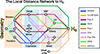 |
Fig. 1. Conceptual overview of the Local Distance Network, a many-routes approach. Different methods for distance determination may connect the absolute scale determined by geometric means to H0. A nonexhaustive list of baseline linkages discussed in the literature or the paper is labeled on the right. Links to geometric distances provided by masers, DEB, and parallaxes are indicated as available in our analysis. Background rectangles in orange, light blue, and gray indicate where Rung 1, Rung 2, and Rung 3 of a traditional distance ladder would fall. Unlabeled tick marks represent groups (Fornax & Virgo for the TRGB to SBF, Coma for FP). Example references: Riess et al. (2022b, SH0ES), Freedman et al. (2025, CCHP), Anand et al. (2021, EDD), Anand et al. (2024b, Pop-II), Pesce et al. (2020a, MCP), de Jaeger et al. (2022, Pop-I), Kourkchi et al. (2020, CF4), Said et al. (2025, DESI), Vogl et al. (2025, adh0cc). Appendix C.1 replicates a subset of these routes. |
2. Methodology
2.1. The Local Distance Network
The goal of measuring accurate and precise distances well into the Hubble flow (D ≳ 100 Mpc) to directly and empirically determine H0 requires the overlapping use of multiple techniques, a combination traditionally referred to as a “distance ladder.” The primary need for this approach is that geometric distance measurements have been limited in range (D ≲ 10 Mpc, and most often D ≲ 100 kpc), while long-range indicators, such as type-Ia supernovae (SNe Ia), are too rare to provide enough examples within reach of geometric distances. Historically, measuring H0 thus required a rather large number of methods and combinations of inhomogeneous datasets (e.g., Freedman et al. 2001; Sandage et al. 2006). Significant improvements in precision and accuracy have since been achieved by streamlining distance ladder setups, focusing on high-quality and maximally homogeneous datasets while maintaining tight control of systematic errors by using the same instrument across rungs to cancel flux calibration offsets. An example is the three-rung “SH0ES” distance ladder Riess et al. (2009a), which calibrates classical Cepheids (henceforth, Cepheids) as standard candles using distances measured by geometrical methods (i.e., higher precision MW parallaxes, detached eclipsing binaries in the Magellanic Clouds, the megamaser distance to NGC 4258), and, in turn, calibrates SNe Ia luminosity using distances to their host galaxies measured using Cepheids observed exclusively using the Hubble Space Telescope (HST). Finally, SNe Ia luminosity distances in the Hubble flow and their redshifts determine H0 (see Fig. 10 in Riess et al. 2016). Such streamlined approaches provided significant benefits in terms of robustness and precision, in part because they avoided potentially correlated systematics, ultimately leading to the Hubble tension as discussed today.
In recognition that the tension may be indicating something profound, greater reliability has been sought through an increasing number of different methods, sources, and measurements. These provide multiple, interrelated constraints for the same or different astrophysical sources, resulting in partially independent paths to H0. Many of these approaches replace certain steps with alternative methods, sources, or calibrators. For this reason, we believe it is appropriate to consider these tools in aggregate to comprise a “Distance Network,” illustrated schematically in Fig. 1, to better convey the interdependence of these methods. While such a goal was considered “lofty” and potentially unreachable more than a decade ago (see de Grijs 2013, and Fig. 1 therein, originally credited to Ciardullo 2006), the improvements to the systematics of several distance measurement techniques—inspired not least by the Hubble tension—now provide a wealth of robust information that allow the base on which the local measurement of H0 rests to again “diversify.”
The Distance Network provides two critical advantages on the path to a more accurate measurement of H0: robustness (to reduce systematic errors) and statistical advantage (to reduce statistical uncertainties). Systematic errors can be recognized by the redundancy of methods allowing for analyses that “leave one out.” At the same time, redundancy offers the means to reduce statistical fluctuations through covariance-weighted averaging. Informally, method combination and robustness has been evaluated through the display of “whisker diagrams” which separate measurements of H0 by the combination of techniques they employ. Intermediate measure comparisons have also been made, most importantly by comparing multiple ways to measure distances to specific SN Ia hosts, each calibrated by the same geometric source (e.g., Cepheids, TRGB, Miras, and JAGB), though these involve only a fraction of the available data (Riess et al. 2024). Formal covariance-weighting and combining has been attempted for only a limited set of indicators (Riess et al. 2022b).
In this paper we introduce an approach to the Distance Network that obviates these shortcomings. By combining existing measurements at the component level, rather than in terms of the resulting value of H0, into a common, statistically rigorous framework encompassing a broad range of methods, this approach yields a combined value of H0 with an uncertainty that reflects all available information. Within this framework, we will also be able to include or exclude different subsets of measurements, thus identifying possible outliers. We will be able to inspect residuals at different levels, verifying whether they are consistent with their stated accuracies.
2.2. Nomenclature and definitions
Given the intricate interrelations between different methods and measurements and the complexity of the resulting framework, we defined at the outset a set of terms, following past usage as closely as possible, that we used to formulate our approach. The principles underlying the various methods alongside the datasets used are presented in Sect. 3 and Appendix A.
2.2.1. Anchor
Any object, or collection of objects, whose distance is directly determined by geometric means, such as parallax or measurements of orbiting systems, and is used to calibrate the distances of other indicators. Anchors set the absolute scale of the Distance Network; all other distances, with a few exceptions (Sect. 3), are measured relative to this scale. The anchors used in this analysis include NGC 4258, through Keplerian motion of circumnuclear masers; the Magellanic Clouds, through detached eclipsing binaries (DEBs); and the collection of Milky Way Cepheids, through trigonometric parallaxes. The Milky Way uniquely provides distances to individual objects rather than a single extragalactic system, mostly measured by the ESA Gaia mission, which are then combined into a single calibration of the Leavitt Law for Galactic Cepheids. To a lesser extent, depth effects are also present in the Large Magellanic Cloud (LMC) and Small Magellanic Cloud (SMC), but may be corrected through the use of empirical geometric modeling fit to the collection of DEBs. In the traditional distance ladder, these anchors of geometric measures are often referred as the first rung.
2.2.2. Primary distance indicator
An astronomical feature that can be measured or calibrated directly using the aforementioned geometric means. Examples include the luminosity of the intercepts of the Leavitt Law of Cepheids or oxygen-rich Mira variables, as well as the luminosities of the tip of the red giant branch (TRGB) or the J-region of the asymptotic giant branch (JAGB).
2.2.3. Host
An object, typically a galaxy, whose distance can be estimated from its properties via a primary distance indicator. Relevant hosts include one or more secondary distance indicators and by means of their identical distance, enable absolute calibration of the secondary indicator (i.e., converting relative distance to true distance). In the distance ladder, these are often referred to as the second rung.
2.2.4. Secondary distance indicator
An astronomical feature that can be measured in more distant systems (“hosts”) and ideally reach out to Hubble flow systems. Secondary distance indicators used here include the luminosity of Type Ia and Type II supernovae (SNe Ia, SNe II), based on the measurement of objects in nearby hosts; the Tully-Fisher (TF) relation, which relates a spiral galaxy’s luminosity to its velocity width; the standardized luminosity of surface brightness fluctuations (SBFs); and the fundamental plane (FP) of elliptical galaxies, calibrated using its properties in the Coma cluster.
2.2.5. Calibrator
An astronomical object used in the calibration of a secondary distance indicator, such as SNe Ia, SNe II, and galaxies with luminosity estimated via TF or SBF relations. A Calibrator is in a host (or simply is a host, when the secondary distance indicator is based on the whole galaxy), and its distance is constrained by the host distance.
2.2.6. Group
A grouping (group or cluster) of galaxies that are assumed to be at a common distance, with appropriate dispersion due to depth effects. Group membership is used to obtain a distance estimate for some Calibrators, including SBF calibrators in Virgo and Fornax and FP calibrators in Coma.
2.2.7. Direct distance determination
A method that yields the distance to an astronomical object directly, without relying on intermediate calibration steps. Such methods are used to determine the distance of anchors, via trigonometric parallaxes (in the Milky Way), the orbital signatures of red giant stars in DEB (LMC, SMC), or the relation between line-of-sight and angular velocity fields in a system of masers (NGC 4258). However, direct distance determinations can sometimes be applied to astronomical objects in the Hubble flow (see next item) and thus provide a direct constraint on H0. Examples include maser systems similar to that in NGC 4258, which yield an angular diameter distance by modeling their recession and angular velocity fields, and SNe II calibrated via the expanding photosphere method (EPM), which determines distance by comparing angular size measured from surface brightness and color temperature to physical size determined from the evolution of the velocity profile.
2.2.8. Hubble flow system
(also called Tracer) An object at sufficiently large distance such that its cosmological redshift can be determined with good accuracy from its measured velocity; together with an angular or luminosity distance determination, such objects provide constraints on the value of H0. Tracers used here include SNe Ia, SNe II, galaxies with luminosity distances estimated from TF or SBF relations, megamasers, and elliptical galaxies via FP. The angular or luminosity distance can be determined using a primary or secondary distance indicator, or through a direct distance determination. Consistent with most determinations of the local value of H0, we limit our analysis to redshifts large enough to reduce the impact of correlated flows due to large-scale structure, generally z > 0.01 or z > 0.023, and small enough (z ≲ 0.15) that a simple, kinematic form of the redshift–distance relation suffices. In practice, the effective redshift range for Hubble flow systems follows the relevant literature and depends on the tracer; tracers that require resolved galaxy images, such as SBF, typically occupy a lower redshift range than SNe Ia.
2.2.9. Use of variance and covariance
For each measured quantity, the original sources often define an uncertainty, which can be the combination (in quadrature) of several terms. For example, the uncertainty in a TRGB-based measurement of the distance to a host galaxy (calibrator) may combine at least three terms: the uncertainty in the geometric distance to the anchor, such as NGC 4258; the uncertainty in the apparent magnitude of the TRGB in the anchor; and the uncertainty in the TRGB of the calibrator itself. However, several of these terms may be in common with other data. For example, all distance estimates anchored to NGC 4258 share the variance associated with its geometric distance measurements, and all TRGB distances estimated relative to NGC 4258 share the uncertainty of the apparent TRGB magnitude determination in this galaxy. In order to make use of more than one such measurement, these terms must be included as covariances between the relevant data and thus added as off-diagonal elements to a full covariance matrix of the data system. More details are given in the description of the equations in Appendix B.
Based on the need to define covariance and successfully leverage a broad range of distance indicators, it is necessary to restrict the use of measurements to those with direct traceability to well-defined sources. Likewise, direct linkages assume consistent measurements between sources (e.g., Cepheids in an anchor and an SN Ia host), a reasonable assumption when both employ the same telescope and instrument. In contrast, the combination of measures from different telescopes and instruments involves substantial covariance (most certainly from different zero points) whose characterization is rarely provided in publications and is beyond the scope of this work to define. The above serve as “quality cuts” for the inclusion of data in the distance network. As an example, we make use of TRGB measurements in hosts calibrated with NGC 4258, where both are identically measured with HST (or JWST). However, we do not combine ground-based and space-based calibrations.
2.3. Distance Network architecture
Given very few assumptions3, the measures and concepts presented above may be linked together as a system of equations, as we show below and in Appendix B, which we refer to as the Distance Network. The multiplicity of data (see Sect. 3 and Appendix A) means we can optimize the system by introducing free global parameters. The wealth of sources, methodologies, and distance indicators also provide important additional and complementary information which can help strengthen the distance ladder or can contribute to constrain H0. For example, the distance to a given supernova host can be measured via different methods (TRGB, Cepheids, JAGB, Miras) depending on which observations are available for that galaxy, and each method can be related to a different anchor. However, these determinations are not independent, as explained under “Use of variance and covariance” in Sect. 2.2. The full Distance Network is illustrated in Fig. 2.
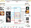 |
Fig. 2. Complete Distance Network, with all possible pathways illustrated. Anchors are objects that establish an absolute scale based on the methods shown to their left. The primary distance indicators (Cepheids, TRGB, Miras, and JAGB) transfer the absolute scale to hosts (i.e., galaxies), the ensemble of which calibrates secondary distance indicators in the Hubble flow (tracers). Exceptions are Megamasers and astrophysically modeled SNe II, both of which serve as primary distance indicators and are capable of reaching the Hubble flow without intermediate steps. Green arrows illustrate direct connections between anchors or tracers and the method used to determine the absolute scale. Blue, violet, yellow, and red arrows show which calibrators constrain host distances; line width qualitatively distinguishes the attainable precision. Among hosts, rectangles qualitatively indicate overlap among objects measured via multiple methods. Diamond shapes represent groups. Dark gray arrows tie subsets of hosts whose distance is constrained by different calibrators to tracers. Any given arrow may represent multiple datasets, for example, HST or JWST photometry of Cepheids or optical versus infrared photometry of SNe Ia. The number of hosts is labeled for Cepheids, TRGB, JAGB, and Miras, with the number of hosts exclusively available to each method shown in parentheses. |
Within the approximations of the present analysis, all equations are linear (or linearized), and all probability distributions are Gaussian in magnitude, distance modulus, or log10(H0). Due to shared calibration sources among primary or secondary distance indicators, a covariance matrix with off-diagonal elements provides a useful method for proper accounting and weighting. The optimization procedure is that of a generalized linear least squares problem. The global solution to this problem provides best-fit values for the underlying parameters of the Distance Network as well as their uncertainties, most notably the distance moduli of included host galaxies, absolute magnitude calibrations, and the Hubble constant. These parameters include log10(H0), the distance moduli to host systems, μhost, ℋ, and groups included in the host data, μ𝒢, as well as the reference magnitudes for each type of calibrator, Mref, 𝒯. The full description of the system of equations and the covariance matrix is given in Appendix B. The employed datasets are listed in Table 1, described briefly in Sect. 3, and shown in greater detail in Appendix A.
Distance Network datasets.
2.4. Implementing the Distance Network
2.4.1. Selecting the baseline
There was strong consensus among the workshop participants, which is also shared more broadly within the community, that not all data, measurements, and tools are viewed with equal confidence. For this reason, we decided to produce a “baseline” result based on all methods which enjoy the broadest and highest level of confidence (sometimes referred to in the literature as “gold standards”), along with variants to the baseline that incorporate additional methods or datasets, or exclude certain data in order to reflect a broad range of minority viewpoints and explore the robustness of the results. To reach a true consensus for the baseline and variants, we adopted a collaborative, methodologically inclusive approach during the ISSI workshop (i.e., “What’s under the H0od?”). Prior to analyzing any combined fits, we engaged in extensive discussion of the various available methods, the choice of datasets (for instance, Cepheids from HST, TRGB distances from JWST, etc.), distance calibrators, and the systematic uncertainties involved in the determination of local distances and H0. These included both classical and emerging techniques, ranging from geometric anchors (e.g., megamasers, Gaia parallaxes, and detached eclipsing binaries) to stellar standard candles (e.g., Cepheids, TRGB, Miras, and JAGB), as well as other methodologies such as SBFs from HST and JWST and the FP from DESI. We also carefully reviewed the use of Type Ia and Type II supernovae, which extend the distance ladder into the Hubble flow. In particular, we examined various SNe Ia datasets (e.g., Pantheon+, CSP, and NIR-only samples) as well as SNe II determinations based on both the standard candle method and spectral modeling.
A key element of this process was a series of open, expert-led discussions in a plenary setting, during which participants evaluated the strengths, systematics, data availability, and limitations of each method and dataset. Following these in-depth assessments, we held anonymous ballot votes to determine the configuration of the baseline analysis and well-motivated variants thereof as well as configurations that should be excluded entirely.
The first vote identified the primary and secondary distance indicators and methods considered most technically mature and broadly supported (see Table 2). In a second vote, we decided on specific combinations, methodological choices, and alternative calibrations, resulting in a comprehensive suite of variants; see Table 3. Methods were included in the baseline if they garnered more than half the total votes, including abstentions, as indicated by the horizontal lines in Tables 2 and 3. All votes were taken prior to deriving a value of H0, and their outcomes were considered binding. The datasets included in the baseline configuration are listed in Table 1 and discussed in detail in Appendix A. Where multiple datasets were available in principle, preference was given to datasets that had been fully published and/or have been most widely adopted. Alternative datasets, notably of SNe Ia (i.e., Pantheon+ versus CSP versus BayesSN), were included as variants.
Ranking of distance calibrators.
Ranking of secondary distance indicators.
This process aimed at identifying the most widely supported and robust measurement paths based on current data and understanding, not at enforcing a single value of H0. The resulting baseline, variants, datasets and code provide a flexible framework to assess the stability and reliability of the derived consensus H0 value under well-motivated methodological changes. This structured approach reflects the collective judgment of the experts present at the workshop, and provides a reproducible path forward for future analyses. Hence, “consensus” here refers to an a priori agreement on how a Distance Network should be constructed in terms of methods, datasets, and their combinations, rather than on the outcome, which was not known when the process was fixed.
In summary, the baseline analysis reflects the scientific consensus among workshop participants concerning the optimal combination of datasets and methodologies as established prior to obtaining results. It should be emphasized again that the vote served primarily to establish a consensus on the level of maturity of diffeerent methods; no method was excluded through this process, and all data remain available to run the Distance Network if different combinations are desired. Variants of the baseline analysis were performed to test the robustness of the result to individual methods, to different datasets corresponding to identical methodologies, and to quantitatively explore “hypothesis-driven” setups that combine multiple elements deviating from the baseline. Further detail on the process of selecting variants is provided in Sect. 2.4.2 below.
2.4.2. Selecting variants and other methodological choices
We defined analysis “variants” to explore the sensitivity of the H0 determination to well-motivated modifications in the analysis setup. Possible variants were identified through brainstorming and subsequently discussed for their merits and weaknesses. These variants serve as internal consistency tests (or “null tests”), helping to assess the robustness of the baseline result under plausible changes to inputs or methodology. Considerable discussion was involved in ensuring that variants were well-motivated prior to knowing their impact on H0. We specifically avoided combinations targeting maximal changes in H0, as these would require a posteriori information or intermediate outcomes, potentially becoming prone to confirmation bias. Our process described in Sects. 1 and 2.4.1 was key to taking these decisions well informed by broad interdisciplinary and expert knowledge. In each variant, we furthermore aimed to adequately reflect the current state-of-the-art in the various disciplines by including all datasets sufficiently precise to carry significant weight in the determination of H0. In other words, we omitted datasets or methods only when motivated by a specific hypothesis in order to avoid artificially inflated uncertainties (i.e., caused merely by insufficient data) that would reduce the Hubble tension in an uninformative way not representative of the state of knowledge.
We reiterate that most variants are effectively “null tests.” Their consistency (or lack thereof) serves primarily as a test of robustness of the baseline. In general, they are not fair substitutes for the baseline solution and should always be referenced together with a description of their underlying choices. It is also critical to note that the values of H0 obtained with all variants are highly correlated. They share a large fraction of the underlying data and are therefore expected to differ from each other by much less than the nominal uncertainty. Therefore, quantifying if individual datasets have anomalous pulls on the final result requires a more careful analysis (see Sect. 5 for further discussion).
The variants discussed in this paper can be organized into different categories. We outline these categories in the following.
2.4.2.1. Add-one-in variants
include additional information that was not voted for inclusion in the baseline and is introduced through a step-by-step process. This category can introduce additional anchors (i.e., the SMC) as well as primary or secondary distance indicators. For example, V01 (Baseline+JAGB) adds JWST/NIRCam distances of the JAGB in supernova hosts calibrated to that in NGC 4258. The addition of calibrators to the baseline configuration serves to explore whether these supplementary methods shift or reinforce the baseline results. Furthermore, this category includes the incorporation of alternative distance indicators in the Hubble flow, such as SNe II calibrated via the standard candle method or spectral modeling, the FP from DESI anchored to Coma, and the TF relation as implemented in the Cosmicflows-4 catalog (CF4; Kourkchi et al. 2020).
2.4.2.2. Leave-one-out variants
involve the exclusion of individual methods or calibrators from the baseline configuration, motivated by the hypothesis that there is an undiscovered error in a type of measurement. Each variant is constructed by removing one key element at a time—such as Cepheids, SNe Ia, TRGB, Gaia parallaxes, or NGC 4258—and observing the resulting impact on the derived H0 value. These tests help identify whether any individual dataset or calibrator is significantly impacting the result. This category also includes the exclusion of specific indicators in the third rung, such as SBF, SNe Ia, and masers in the Hubble flow. Since leaving out a given element can implicitly remove other elements (e.g., specific SNe Ia calibrators), we have constructed custom baselines (see below) to separately assess the effect of the implicit (undesired) modification relative to the baseline.
2.4.2.3. Instrument-suspicious variants
explore the impact of removing specific observatories or classes of observations. In particular, we tested the exclusion of all HST or JWST-based observations and of all SNe Ia before 1994. Similar choices, such as excluding all Gaia parallaxes, are included as “Leave-one-out” variants.
2.4.2.4. Hypothesis-driven variants
involve compound configurations motivated by specific physical or observational hypotheses. These include the use of alternative calibrations (e.g., CSP/SNooPy instead of Pantheon+/SALT2 for SNe Ia), different treatments of systematics (e.g., inclusion or exclusion of peculiar velocity corrections, metallicity corrections, or near-infrared (NIR) SN data), and restricted subsets of the data (e.g., only modern SNe Ia or cutting the Hubble flow sample at z > 0.06). Additionally, we included a variant that considered the Cepheid Leavitt law to be independent of chemical composition.
2.4.2.5. Custom baselines
The exclusion of certain measurements can also cause the exclusion of some SNe Ia calibrators. For example, when Cepheid measurements are excluded, only 35 of the 55 SNe Ia calibrators in the baseline can be included, since the other 20 only have determinations of the host distances through Cepheids. The resulting change in the H0 value and uncertainty is due to both the exclusion of the measurements and the change in the SNe Ia calibrator sample. To cleanly separate the two effects, we defined a custom baseline that includes those measurements, but it is restricted to only the SNe Ia calibrators for which other measurements are available. Custom baseline versions are not variants per se; they are only intended to facilitate the interpretation of the results for the corresponding variants.
2.4.2.6. Include everything
We also consider a variant in which all independent methods and data sets are included, to illustrate the accuracy that can be achieved with presently available measurements if systematic effects and other issues are resolved. A secondary variant in this class uses all independent methods except TF, for which the current dataset has excess dispersion. In either version, this variant includes only one set of measurements for SNe Ia, since different measurements are likely correlated (because of astrophysical variance) to a degree that has not been sufficiently quantified in the literature.
2.4.2.7. Additional solutions
In addition to the variant solutions described above, we also consider special solutions designed to test our methodology. These are not “variants” in the same sense as those listed previously, and do not appear in Table 4; they are discussed in more detail in Sects. 5.3.1 and 5.3.2 and Appendix C. They include independent grouping solutions, consistency checks, and emulator solutions. Independent grouping solutions consist of configurations in which two or more fully independent paths through the distance ladder are identified, sharing no common calibrators or intermediate steps. These allow for the construction of entirely separate determinations of H0, such that agreement between them provides a strong consistency check and minimizes the risk of shared systematic effects. They are the analogous to splitting the data in uncorrelated halves or thirds. Two such variants are discussed in Sect. 5.3.1. Consistency checks are employed to make sure that the network results are statistically self-consistent for different paths through it and are further discussed in Sect. 5.3.2. Emulator solutions involve a set of “emulators” designed to reproduce key published results, such as SH0ES, CCHP, and recent SBF analyses, within our unified framework and dataset handling. These configurations serve both as validation tests of our pipeline and as transparent benchmarks for comparison with previous literature, and they may also help explain sources of differences. These are discussed in Appendix C.
Main variants for H0 calculation.
3. Dataset descriptions
The analysis presented in this work is based on a comprehensive set of local distance measurements and their corresponding calibrators, as detailed in Sect. 2 and conceptually shown in Fig. 1. The dataset includes a broad array of distance indicators, spanning geometric anchors, calibrators, and tracers. These are combined using a statistically rigorous framework that accounts for shared systematics and covariances among measurements. To maintain clarity and readability in the main text, we provide here only a brief summary of the datasets used to construct the Distance Network, summarized also in Table 1. Methods employed in the baseline are marked in bold. A more detailed description of the individual measurements, sources, and associated assumptions is given in Appendix A. We employ peculiar velocity corrections as described in Appendix B.3.7.
3.1. Parallaxes
We adopted trigonometric wide-angle parallaxes (henceforth, parallaxes) of Milky Way stars from the early third data release of the ESA Gaia mission (GEDR3; Gaia Collaboration 2016, 2021). GEDR3 parallaxes were corrected for systematics following Lindegren et al. (2021a) and for additional residual offsets as determined for field Cepheids (Riess et al. 2021). GEDR3 parallaxes of open stars clusters were determined using nonvariable member stars (Riess et al. 2022a; Cruz Reyes & Anderson 2023). An additional seven narrow-angle parallaxes of Cepheids based on the HST/WFC3 spatial scanning technique were included (Riess et al. 2018).
3.2. Detached eclipsing binary distances
The distances to both Magellanic Clouds have been determined using helium burning red giants in DEB systems. These distances are determined geometrically as the ratio of the physical stellar radii determined from full orbital solutions to the angular diameters determined by surface-brightness-color relations calibrated empirically using long-baseline interferometry. The distance to the LMC from Pietrzyński et al. (2019) contributes to the Cepheid calibration in the baseline analysis. An analogous distance to the SMC from Graczyk et al. (2020) was considered as part of a variant.
3.3. Megamaser distances
We adopted geometric distance measurements to the anchor galaxy NGC 4258 and four additional galaxies out to the Hubble flow. The distances were determined via very long-baseline interferometric (VLBI) radio-wavelength observations of water megamasers in accretion disks surrounding central supermassive black hole of their host galaxies. Distances were determined by comparing the physical scale of the megamasers determined from a Keplerian disk model to the angular extent of the features (Braatz et al. 2015; Reid et al. 2019; Kuo et al. 2020).
3.4. Cepheids
The Leavitt Law, or Period–Luminosity relation of classical Cepheids (throughout this work: Cepheids) is a well-understood consequence of the dependence of acoustic oscillations on stellar density, the relation between mass and luminosity, and the Stefan-Boltzmann law. The periods of their observed brightness variations link directly to their intrinsic luminosity (Leavitt & Pickering 1912) with particularly small scatter in the infrared, and this is well described by stellar evolution models (e.g., Khan et al. 2025). Distances to Cepheids pulsating in the fundamental mode were measured using the reddening-free NIR Wesenheit magnitudes based on HST photometry published by Riess et al. (2018, 2021), 2022a, 2019, 2022b), Yuan et al. (2022), Breuval et al. (2024), and more recently with JWST by Riess et al. (2023, 2024, 2025). The Cepheid Period–Luminosity relation was calibrated in anchor galaxies using geometric distances in the Milky Way, Magellanic Clouds, and NGC 4258.
3.5. Tip of the red giant branch
The TRGB represents a recognizable feature in the color-magnitude diagram of galaxies that is caused by the nearly constant luminosity of the Helium flash of first-ascent red giant stars, which continue along their evolution toward the Horizontal Branch. The TRGB distances were measured using HST and JWST observations of resolved stars in nearby (D < 30 Mpc) galaxies. These distances were measured by the Carnegie-Chicago Hubble Program (CCHP; Freedman et al. 2019; Hoyt et al. 2021, 2025), the Extragalactic Distance Database (EDD; Tully et al. 2009; Anand et al. 2021), the SH0ES team (Anand et al. 2024a; Li et al. 2024a), and the TRGB-SBF project team (Anand et al. 2024b, 2025). Each team used somewhat different reduction, analysis, and calibration techniques, but we find that the resulting distances are generally consistent across groups, as shown in Sect. 4.
3.6. J-region asymptotic giant branch
The JAGB is a recognizable feature in the NIR color-magnitude diagram of galaxies attributed to post-third dredge-up carbon-rich intermediate-mass AGB stars. The JAGB distances used here are derived from data taken with JWST NIRCam as published by Li et al. (2024b, 2025b, SH0ES) and Freedman et al. (2025, CCHP) (see also Appendix A). In its current implementation, the JAGB method assumes a homogeneous stellar population with a constant average luminosity. Systematic uncertainties, for example asymmetric luminosity functions or metallicity effects, were considered following Li et al. (2024b) and remain a subject of research (e.g., Zgirski et al. 2021; Magnus et al. 2024; Lee et al. 2025).
3.7. Mira distances
Miras are high-amplitude long-period variable AGB stars that obey period–luminosity relations. We use a sample of 3 Mira host galaxies consisting of the geometric anchor NGC 4258 (Huang et al. 2018) and two SNe Ia calibrator galaxies, NGC 1559 and M101 (Huang et al. 2020, 2024), hosts of SN 2005df and SN 2011fe, respectively. All observations consisted of at least 10 epochs of HST WFC3/IR time series photometry spanning a minimum of one year, and distances were obtained using the Mira period–luminosity relation in the F160W bandpass.
3.8. Type Ia supernovae
Type Ia supernovae are standardizable candles whose light curve information (e.g., the duration) can be related to their intrinsic magnitude. We incorporate five different SNe Ia datasets, ranging from optical to NIR wavelengths and spanning different SNe Ia modeling methodologies (Spectral template PCA with SALT2, SALT3, and SNooPy v2.7, and template-free with BayesSN). Four of these datasets are used in the Hubble flow: (1) Pantheon+ (optical) with SALT2 (Scolnic et al. 2022; Brout et al. 2022b), (2) Carnegie Supernova Project (CSP) I & II (with SNooPy v2.7; Burns et al. 2011; Uddin et al. 2024), (3) template-independent distances in NIR (Galbany et al. 2023), (4) optical+NIR samples processed with BayesSN (Dhawan et al. 2023). A fifth dataset of 13 SNe Ia is used to calibrate the distance to the Coma cluster (Scolnic et al. 2025).
3.9. Type II Supernovae (SNe II)
Several methods exist to standardize SN II magnitudes and derive distances (see de Jaeger & Galbany 2024). In particular, the Standard Candle Method (SCM; Hamuy & Pinto 2002) standardizes SN II luminosities based on correlations with photospheric velocity (from Hβ) and color. We use a sample of 89 SNe II in the Hubble flow at z > 0.01 as well as 14 calibrator supernovae from de Jaeger et al. (2020a, 2022), compiled from CSP-I, LOSS, SDSS-II, SNLS, DES-SN, and SSP-HSC (de Jaeger et al. 2017b,a, 2020a).
3.10. Expanding photosphere method of Type IIP supernovae
We adopted distances of Type IIP supernovae (SNe IIP) determined by astrophysical modeling via the tailored EPM from Vogl et al. (2025). Such distances relate the angular extent of SNe IIP measured from light curves to their physical expansion determined by radiative transfer modeling of optical spectra (Vogl et al. 2020; Csörnyei et al. 2023b). The EPM can be applied to SNe IIP in the Hubble flow without requiring additional calibration, although it depends on the accuracy of the underlying astrophysical modeling.
3.11. Surface brightness fluctuations
Spatial fluctuations in the surface brightness of an otherwise smooth galaxy arise from the statistics of the discrete number of stars per pixel. The amplitude of these fluctuations depends inversely on the distance of the galaxy, as well as on age, metallicity, and other properties of the stellar population. For galaxies with evolved stellar populations, the SBF method can be calibrated through an empirical relation between the intrinsic magnitude of the fluctuations and the galaxy’s integrated color, used as a proxy for the stellar population properties. SBF measurements in the NIR are particularly useful because the fluctuations are bright at these wavelengths and can be well calibrated using optical colors. For this study, we use a sample of 61 HST WFC3/IR SBF elliptical galaxy distances reaching out to 100 Mpc (Jensen et al. 2025, 2021; Blakeslee et al. 2021); distances to the 14 calibrators in the Virgo and Fornax galaxy clusters are based on TRGB (see Appendix B.3.3).
3.12. Fundamental plane
The distance to an elliptical galaxy can be estimated by means of the FP relationship between central velocity dispersion, effective radius, and surface brightness. Fundamental plane distances were measured using the Dark Energy Spectroscopic Instrument (DESI) Early Data Release, analyzing 4191 early-type galaxies within 0.01 < z < 0.1 with photometry from the DESI Legacy Imaging Surveys and spectroscopic velocity dispersions from DESI observations (Said et al. 2025). The FP zero point calibration was established using a collection of galaxies in the Coma cluster, with the distance of the latter constrained by 13 SNe Ia within Coma analyzed by Scolnic et al. (2025), as well as an additional (fixed) constraint from SBF (see Appendix B.3.8).
3.13. Tully-Fisher
The TF relation relates the rotation velocity of spiral galaxies (determined with HI line widths) to the total intrinsic luminosity. TF data were obtained from the Cosmicflows-4 catalog (Kourkchi et al. 2020), which compiled HI line widths, redshifts, and photometry for ∼10 000 spiral galaxies across the full sky, out of which we use 3400 galaxies with complete infrared photometry (as recommended by Boubel, priv. comm.). The TF relation zero-point has been recalibrated within the Distance Network using calibrator galaxies identified in Boubel et al. (2024a), with systematic corrections applied by Scolnic et al. (2024).
4. Baseline results
The baseline solution for the Distance Network as illustrated in Fig. 3 yields
 (1)
(1)
As described in Sect. 2.4.1, this solution includes SNe Ia, SBF, and megamaser measurements as Tracers. The distances to hosts of SNe Ia and SBF calibrators are obtained from the solution of the full Distance Network, incorporating measurements based on TRGB and Cepheids from the sources described in Sect. 3, with the Milky Way, LMC, and NGC 4258 as anchors for Cepheid distances4. SNe Ia measurements are from the Pantheon+ sample, and peculiar velocity corrections in the Hubble flow are based on the 2M++ model (Carrick et al. 2015). This solution has an overall χ2 of 0.9879 per degree of freedom, indicating broad agreement between the estimated uncertainties—all based on original sources—and the statistical properties of the solution. Note that the value of χ2 does not include degrees of freedom associated with SNe Ia and SBF tracers in the Hubble flow. In our methodology, we solve separately for the Hubble flow intercept for SNe Ia and SBF tracers in the Hubble flow—as well for others that are not included in the baseline solution, such as SNe II and TF tracers—and only the intercept is included in the final Distance Network solution. It can be shown that, apart from a separation of the χ2 values, this approach is equivalent to directly including the Hubble tracer equations into the Distance Network (see also Appendix B.3.6).
Figure 4 shows the residuals of host distances, estimated from the network solution, grouped by methodology. Each grouping, identified by a different color, refers to a specific combination of primary distance indicator, anchor, and source, as indicated in the labels below the group. The error bars shown correspond to the uncertainty of the specific distance measurement for that host, not including terms that are covariant with the other elements of the group. For example, each Cepheid measurement is shown with the uncertainty of the Period–Luminosity intercept for that galaxy, which reflects the expected scatter of residuals within that group. The color-shaded band for each group shows instead the uncertainty associated with common error terms for that group, i.e., the anchor uncertainty and the uncertainty in the indicator measurement (TRGB magnitude or Cepheid Period–Luminosity intercept) for that anchor, combined in quadrature; this term is indicative of the likely scatter of the average of the group—shown by the corresponding horizontal line at the center of the band—with respect to zero5. As can be seen, the distribution of residuals is consistent with expectations, with no significant deviation from the published uncertainties for any subset of data.
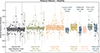 |
Fig. 4. Residuals for each category of host distance measurements from the Baseline solution. Each panel represents a group of measurements of host distances that share the same method, anchor, and authors, and shows the deviation of those measured host distances from the full Distance Network value. Error bars represent the individual uncertainty of each measurement, while the shaded regions for each group shows the common (fully correlated) uncertainty due to the reference system. |
A closer look at the residuals for Cepheids clearly shows that all anchors yield distances consistent with one another, as well as with TRGB-based distances. The systematic offsets (horizontal bars) for Cepheids anchored to the LMC, the Milky Way, and NGC 4258 differ by 0.02 mag or less from the distance network solution. Subsets of TRGB measurements have slightly larger typical offsets, about 0.03 mag, justified in part by the smaller number of systems included in each study; but overall they are in very good agreement, within the expected statistical uncertainties.
Figure 5 shows the distribution of residuals for objects in the Hubble flow as a function of redshift for three classes of objects. The ordinate is the offset in log10(H0) inferred for that specific object; the error bar reflects a combination of the measurement uncertainty (photometric error, error in standardization, and/or uncertainty in the solution, as applicable), the effect of the dispersion in peculiar velocities, the uncertainty in the peculiar velocity reconstruction, and the intrinsic dispersion in the relevant distance indicator, as determined in the original sources from the dispersion in the calibrators. They do not include the calibration uncertainty, which is determined as part of the distance network calibration solution for each group when applicable. The shaded bars at the right show the measured mean and dispersion for each of the three sets of data. Again, both the dispersion in individual measurements and the mean for each subset are consistent with expectations, which represent the direct measurement uncertainties for each value—not including calibration uncertainties. Figure 6 shows the posterior distribution for the global fit parameters for this solution: the absolute magnitude calibration for SNe Ia, the offset in the SBF calibration, the estimated distances to Virgo and Fornax, and the value of H0. These are based on finite-length chains extracted from the probability distribution of the solution, and the values of the parameters may be slightly different from the analytically calculated results.
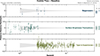 |
Fig. 5. Residuals in distance modulus as a function of redshift for objects in the Hubble flow in the Baseline solution. Error bars reflect the individual source scatter, without the common calibration uncertainty. The shaded region in each plot indicates the effect of a velocity uncertainty of 250 km s−1. The bars at the right show the mean and dispersion for each group of sources and the calibration uncertainty, which is a common error mode for all points in each panel. |
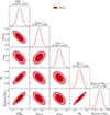 |
Fig. 6. Corner plot for the baseline solution illustrating the correlations between H0, the calibration of SNe Ia and SBF, and the distance to Fornax and Virgo, which contribute to the SBF calibration. The parameters use the naming convention of Appendix B.3.1. Deviations from the analytically calculated result are due to the numerical precision of a finite-length chain. |
The solution for the baseline Distance Network yields the most accurate direct H0 measurement to date, with a relative uncertainty of 1.09%, including systematic uncertainties. It agrees to much better than the 1σ uncertainty with previous determinations of H0 by the SH0ES team (Riess et al. 2022b). The relative uncertainty of this result improves by ≳13% over updates by the SH0ES team based on cluster Cepheids (Riess et al. 2022a) and sibling SNe Ia (Murakami et al. 2023), and by ∼7% compared to the most recent SH0ES update provided by Breuval et al. (2024), which furthermore incorporated the SMC as an additional anchor. As shown by Riess et al. (2022b), integrating TRGB distances into the fit strengthens the result, but does not cause it to deviate strongly. In the baseline case, this finding extends to the inclusion of distant megamasers and the SBF measurements. More generally, we find excellent agreement with most previous literature results based on direct measurements, as we show in Fig. 7—including most of the studies corresponding to the individual distance ladders that can be constructed within the Distance Network. We explicitly investigate the similarities and differences with respect to previous literature results that are part of the Distance Network in Appendix C, where we also showcase what is necessary to obtain the results with lower central values in H0. We also find great agreement with the recent TDCOSMO results from Tdcosmo Collaboration (2025), which give  and are compatible at ∼0.5σ.
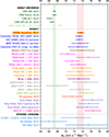 |
Fig. 7. Comparison of the baseline result with previous literature results based on early Universe indirect inferences using the flat ΛCDM model, based on direct measurements in the late Universe, and based on strong lensing results (which involve additional modeling). |
The consensus H0 measurement differs from the indirect, ΛCDM-dependent measurement based on the CMB anisotropies of 67.24 ± 0.35 km s−1 Mpc−1 (Camphuis et al. 2025, Eq. (54)). This corresponds to a statistical significance of 7.1σ.
5. Variants
Exploring variants to the baseline solution serves multiple purposes. First, several available methods and datasets were not included in the baseline solution, for various reasons—primarily because of maturity of analysis or questions about uncertainty estimates. These data can still be used to highlight potential issues with the baseline solution, or point toward future research directions. In some cases, additional observations may eventually justify including these methods in the baseline. Second, it is informative to assess what happens to both the value and uncertainty in the Hubble constant when different categories of data are included or excluded in the solution. Third, some methods—for example SNe Ia—can be included in several different ways; different filters, different light curve analysis, or different redshift selections. Finally, it is useful to consider a solution that includes all available, independent data and methods to assess the potential precision achievable with existing data once the remaining analysis issues are resolved. We stress that our process determined the baseline analysis as the primary solution prior to obtaining any results on H0. Variants in these categories are defined in Sect. 5.1, and the results discussed in Sect. 5.2.
Separately, we also consider two additional sets of consistency checks presented in Sect. 5.3. One builds fully independent, “orthogonal” paths capable of determining H0 to verify that no single path/method dominates the Distance Network (see Sect. 5.3.1). The other employs a variety of different, albeit not independent, paths through the data to verify that their statistical properties are consistent with expectations (see Sect. 5.3.2). These checks serve to demonstrate the statistical consistency of the baseline solution with all possible configurations. Replications of results presented in the literature provide additional consistency checks of our methodology and are presented in Appendix C.
Some general considerations pertain to all these analyses and their interpretation. First, the baseline and variants were defined and classified before considering the resulting values of H0. Very minor changes were introduced afterward if required by updated data availability, albeit without changing the definition of the baseline. Second, most “variants” should not be regarded as alternative, equally valid solutions. Rather, their role is to illustrate the statistical properties of the data, identify potential problems, and/or reinforce their validity. This is especially true when considering the consistency checks, which are designed specifically so that each path uses only a small fraction of the available data and thus by construction has a large nominal uncertainty, which is in no way representative of the uncertainty in H0. Third, the results of all variants are highly correlated because they share large portions of data. An exception are the orthogonal paths in Sect. 5.3.1, which serve as consistency checks. Hence, the scatter between variants is expected to be much smaller than their error estimates.
5.1. Description of variants
The following is a short description of the main variants included in Table 4. Specific sources of data products are provided in the text and in Appendix A.
5.1.1. Baseline
5.1.2. Add-one-in variants
5.1.3. Leave-one-out variants
5.1.4. Instrument-suspicious variants
5.1.5. Custom baselines
5.1.6. Hypothesis-driven variants
5.1.7. Include everything
5.2. Overview of results based on variants
The results of the baseline and all variants are illustrated in Fig. 8 and reported in Table 4. For each variant we report the resulting value of H0 and its 1-σ uncertainty, the number of degrees of freedom, the reduced χ2 for that solution, and PTE, the probability to obtain a larger value of χ2; a very small value of PTE indicates an anomalously large χ2, and is only seen in variants that include the TF method, as discussed in what follows. When appropriate, we also report Δσ, which is the variation in H0 with respect to a reference value in units of its expected dispersion. This quantity is computed only when a variant is a strict subset or superset of another, and it is usually referenced to the baseline variant except for those variants that have a custom baseline; the expected dispersion is the quadrature difference of the two variants being compared. (See Gratton & Challinor (2020) for the methodological details).
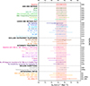 |
Fig. 8. Baseline and variants results from Table 4. For some variants, a labeled change has a secondary consequence (i.e., removing the identified primary distance indicator also results in the loss of calibration to some SN Ia). In these cases a dashed line immediately below such variants provides a custom baseline–i.e., the same SNe are removed before the removal of the primary indicator–is shown to provide a custom reference of the impact for that variant (see text for details). |
All variants yield results consistent with the baseline, typically varying only slightly from the baseline result; the dispersion of central values is 0.400 km s−1 Mpc−1, or 50% of the baseline’s 1σ uncertainty. Since the baseline and its variants are highly correlated due to shared datasets and methodologies, a scatter significantly below 1σ is expected. The absence of outliers among the variants demonstrates that the results are not driven in any particular direction by any one dataset or methodology, or any of the hypothetical systematics explored. For example, variants V08, V10, and V13 demonstrate that the central value of H0 is not dominated by Cepheids (V08), parallaxes mainly from Gaia (V10), or SNe Ia (V13). Figure 8 also readily identifies differences in constraining power brought by various methods: the largest increases in the error on H0 are seen in V08 (no Cepheids), V13 (no SNe Ia), and V16 (no HST). This underlines the crucial precision provided by Cepheids, SNe Ia, and HST observations, whereas the insensitivity of the central value on H0 demonstrates that neither dominate the result. The exploration of such variants establishes robustness of the baseline result and demonstrates that the Distance Network is enhanced by the joint consideration of complementary methodologies. It further underlines that the different methodologies reinforce and strengthen each other, resulting in improved accuracy thanks to the DN approach.
5.2.1. Adding one class at a time
Variants V01 to V07 each add one category of objects or methodology to the baseline solution; these include JAGB, Miras, the FP of elliptical galaxies, empirically and astrophysically calibrated SNe II, TF, and the SMC as an additional anchor. For all cases except the TF relation, the impact on the solution is negligible, with the central value of H0 changing by 0.2 km s−1 Mpc−1 or less (25% of the 1σ uncertainty), and the uncertainty remaining constant or decreasing slightly. Including astrophysically calibrated SNe II (V05) leads to the most significant improvement to the uncertainty, by 8.5% to 0.74 km s−1 Mpc−1; however, this method being relatively new, its systematic uncertainties are not yet fully quantified (Vogl et al. 2025).
Including the TF relation raises H0 by almost 0.5 km s−1 Mpc−1 (∼60% of the baseline error), and yields a reduced χ2 significantly larger than unity (1.4712). The increase in H0 is consistent with the results of the recalibration of the TF relation by Scolnic et al. (2024). Inspection of the residuals shows that the anomalous value of χ2 is caused by the dispersion in predicted magnitude for TF calibrators, whose empirical scatter significantly exceeds the assumed intrinsic dispersion, particularly at the bright end. Uncertainties in host distances are subdominant and unlikely to play a role in this comparison. We conclude that the internal dispersion currently assumed for the TF relation is likely underestimated, and recommend avoiding the inclusion of TF results until its intrinsic dispersion can be reevaluated.
5.2.2. Leave-one-out variants
Variants V08-V18 each remove one class of measurements or a subset of data from the solution. Most variants do not change the central value of H0 much, with the exception of V08 (no Cepheids), which drops it by almost 1 km s−1 Mpc−1 to 72.51 km s−1 Mpc−1, and V12 (no NGC 4258), which decreases it to 73.08 km s−1 Mpc−1. Comparing V08 and the corresponding custom baseline (V08B) clearly identifies that the shift in the no-Cepheids variant (V08) is driven by the implicit exclusion of 20 calibrator SNe Ia rather than by the Cepheids themselves. Analogous effects on H0 induced by subsampling SNe Ia calibrators have been extensively discussed in Riess et al. (2024). Accounting for this effect leaves a difference of merely 0.352 km s−1 Mpc−1 (44% of the baseline error) due to excluding Cepheids.
Some variants yield significantly increased uncertainties on H0. Excluding Cepheids (V08) increases the uncertainty from 0.81 to 1.30 km s−1 Mpc−1, and comparison with the uncertainty of the custom baseline V08B (0.87) reveals that this increase is truly driven by the exclusion of Cepheids rather than the implicitly removed 20 SNe Ia calibrators. More modest increases occur for the variants without NGC 4258 as anchor, or when TRGB measurements are excluded. This is simply a reflection of the reduced constraining power caused by the exclusion of a broad class of measurements. Excluding either the Milky Way or the LMC as anchors has less impact, as each exclusion leaves two anchors for Cepheids, and does not affect the TRGB, which is only calibrated via NGC 4258. The most dramatic impact is associated with the exclusion of all SNe Ia; this increases the uncertainty to 1.79 km s−1 Mpc−1, more than a factor of 2 above the baseline, illustrating the strong constraining power of SNe Ia, which remain the most powerful way to measure the local value of the Hubble constant. When SNe Ia are excluded from the baseline, the primary constraint on H0 is based on the SBF measurement. Even in this case, the central value of H0 is changed only little, although one naturally finds a much larger uncertainty. As an illustration, the solution including all other available data but excluding SNe Ia in the Hubble flow—formally not a variant, since it does not satisfy the criteria established during the Workshop—yields 75.29 ± 0.93 km s−1 Mpc−1; despite the higher uncertainty, this value is still 8.1σ away from the CMB value in flat ΛCDM.
The two variants V16 and V17 explore the impact of excluding all calibrator data from either HST or JWST, testing hypothetical broad systematics, such as calibration errors, that might affect either facility. Note that all primary distance indicators as included used space-based data from at least one of the two facilities. Excluding HST also implies excluding the Milky Way and the LMC as anchors, since we do not yet have a calibration for Cepheids in those systems based on JWST data. The solutions with either no HST or no JWST data are not fully disjoint since they share a common anchor, NGC 4258, and many of the Hubble flow tracers, and since the set of calibrators overlap, carrying with them any intrinsic variance in their properties. However, many of the sources of uncertainty in distance estimates are different and independent. The resulting H0 values bracket the baseline, as could be expected, with a difference in line with their respective uncertainties: without HST, 73.75 ± 1.33 km s−1 Mpc−1; and without JWST, 73.00 ± 0.86 km s−1 Mpc−1. Not surprisingly, the uncertainty in the result increases more if HST is excluded, since HST results use three anchors (only NGC 4258 is available for JWST) and more HST observations are available, yet both subsets remain close to the baseline with a difference below 1 km s−1 Mpc−1. The fact that the inclusion of JWST observations favors a higher value of H0 corroborates the conclusion based on host-to-host distance comparisons by Riess et al. (2024) that H0 measurements based purely on HST (Riess et al. 2022b) are not biased high by the limited spatial resolution of WFC3/IR (crowding). Excluding very early SNe (V18), mostly measured with photographic methods, only increases H0 by about 0.2 km s−1 Mpc−1; further excluding all SNe before 2000 would raise H0 by an additional 0.1 km s−1 Mpc−1.
5.2.3. Alternate treatments
Variants V19-V26 show what happens if subsets of data are either excluded or treated differently. For variants V19-V22, we modify the handling of peculiar velocities or redshift selection. In variant V19, we assume that the observed velocities directly represent cosmological redshifts, i.e., we set all peculiar velocity corrections, which are by default derived with the 2M++ model (Carrick et al. 2015), to zero. The value of H0 decreases slightly, to 73.06 ± 0.80 km s−1 Mpc−1, with no meaningful change in the accuracy. Similarly, restricting the redshift range, either by removing the high redshift end (V20, z > 0.06) or the low-redshift end (V21, 0.03 < z < 0.1), changes the value of H0 by up to 0.8 km s−1 Mpc−1; the impact on the accuracy is modest.
Variants V22-V27 are noteworthy because they explore different treatments of SNe Ia, which drive overall precision (see Sect. 5.2.2). Variants V22 and V23 consider different light curve fitters (consistently for both calibrators and tracers), namely SNooPy v2.7 in V22 and BayesSN in V23. Both variants yield slightly higher H0 values with slightly larger nominal uncertainties. The BayesSN variant V23 furthermore yields a higher reduced χ2. Further detail and comparisons with published articles is provided in Appendix C.2, specifically concerning SNooPy in Appendix C.2.1.
Variants V25 and V26 rely exclusively on NIR measurements for SNe Ia (Galbany et al. 2023), in the H and J band respectively. These also yield slightly lower, yet consistent H0 results with slightly larger uncertainties due to the smaller number of calibrators and Hubble flow tracers. Note that we never used SNe Ia measurements from multiple sources (e.g., Pantheon+ and NIR) simultaneously in any solution; doing so would lead to unreliable, likely incorrect results. First, the calibration of SN measurements in different samples are inconsistent, as they are based on different filters, fitting processes, and conventions. More importantly, different measurements of the same SN would share to a large extent the astrophysical variance of the source; therefore we expect such measurements to be significantly correlated in their deviation from the mean, to an extent that, to the best of our knowledge, has not been sufficiently quantified. Since the SNe Ia samples overlap significantly, multiple measurements cannot be included in the same solution in a statistically satisfactory way. To avoid such issues, we take care not to include multiple measurements of the same SNe Ia—whether as local calibrators or as Hubble flow objects—in the same solution. Unless otherwise stated, all solutions exclusively consider measurements collected in the Pantheon+ system (Scolnic et al. 2022).
Another treatment option concerns the covariance between different SNe Ia in the Hubble flow. Several collections of measurements provide covariances between different objects; these can be due to the effect of standardization parameters, or the survey from which data have been obtained. By default, we include such covariances where available. However, Variant V27 deliberately ignores these covariances and assumes (incorrectly) the stated uncertainties to be independent in order to assess the impact that the SNe Ia covariances have on the final result. This results in a miniscule decrease in H0, by less than 0.1 km s−1 Mpc−1, and analogously miniscule decrease in the nominal uncertainty. We conclude that covariances between SNe Ia measurements in the Hubble flow currently have a negligible impact on H0.
5.2.4. “Everything” solution
It is naturally interesting to consider the result of including all available methods into the Distance Network. To this end, we constructed variant V99 by including all available measurements. As noted above, multiple measurements of SNe Ia cannot be combined in a statistically satisfactory way, so that V99 exclusively considered Pantheon+ SNeIa. V99 also incorporates methods with as yet insufficiently well understood systematics, such as SN II with EPM and the TF relation. These results are provided here for completeness, and we recommend that they not be used for further analysis. The resulting value is 73.99 ± 0.70 km s−1 Mpc−1, which lies 8.7σ from the Planck+ΛCDM solution. We recognize that this solution may not be fully reliable, as indicated by the relatively large value of reduced χ2, namely 1.3078 per degree of freedom; indeed, this solution deviates from the baseline more than several others, primarily because of the TF contribution. Since the TF relation contributes the most to the excess χ2, we also include variant V99a, which is identical to V99 except for the exclusion of TF calibrators and tracers. This variant results in H0 = 73.66 ± 0.71 km s−1 Mpc−1, very close to the baseline with a 12% smaller uncertainty (and subpercent precision on H0), has a reasonable reduced χ2 of 0.8943, and lies 8.1σ from the Plank+ΛCDM solution.
The “everything” solution is useful to understanding how elements in the baseline solution compare to the elements not included therein, as well as any covariances among them. Three figures illustrate these points. Figure 9 shows the fit residuals of host and calibrator distances for V99 in analogy with Fig. 4 for the baseline. Figure 10 illustrates the corresponding Hubble flow residuals for V99. A corner plot illustrating covariance among the main global fit parameters of the Distance Network for V99 is shown in Fig. 11.
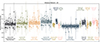 |
Fig. 9. Residuals for host and calibrator distances for the “everything” solution. The groupings, also distinguished by color, correspond to calibrators measured by the same authors with a common method and anchor. The error bars reflect the individual calibrator errors. The shaded areas for each group indicate the combined uncertainty in the anchor distance and its reference value, which are in common for all calibrators in the same grouping. |
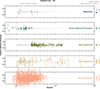 |
Fig. 10. Residuals in log(H0) versus redshift for objects in the Hubble flow for the “everything” solution. Each subplot refers to sources in the same group, measured by the same method. Error bars for individual sources are representative of the expected scatter across sources in the same category and do not include calibration uncertainties for each class. The shaded bars at the right show the mean and dispersion for each category. |
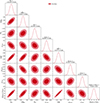 |
Fig. 11. Corner plot illustrating the main optimization parameters for the all-inclusive solution. The naming convention of Appendix B.3.1 is used. Parameters related to individual host distances are not included. Note that this solution is not an alternative result to the baseline solution, but rather it is a variant to check the impact of further data on our result (see also Sect. 5). We show it here to highlight the existing correlations between the various (most important) solution parameters. Deviations from the analytically calculated result are due to the numerical precision of a finite-length chain. |
5.3. Consistency checks
We demonstrated the statistical consistency of the baseline solution by building alternate paths through the Distance Network capable of determining H0. Statistically independent paths are discussed in Sect. 5.3.1, statistically not independent paths in Sect. 5.3.2. Replications of H0 results from the literature are presented in Appendix C.
5.3.1. Orthogonal paths
Orthogonal paths strike statistically fully independent paths across the Distance Network. In creating these paths, we sought to identify configurations capable of achieving similar constraining power. We identified the following two6 orthogonal paths and two extensions of the second path:
-
O1:(MW+LMC+SMC+Ceph+SNIa+FP): This path employs the Magellanic Clouds and Milky Way parallaxes as anchors, calibrates SNeIa using Cepheids, and adds in the FP calibrated in Coma. This yields H0 = 73.11 ± 0.92 km s−1 Mpc−1 with a χ2 = 53.5 and a reduced χ2 of 0.922.
-
O2:(N4258+TRGB+SBF+MM): This path uses N4258 as anchor, TRGB as calibrators, and SBFs as tracers, in addition to megamasers. This corresponds to a modified V07 (baseline+SMC) from which all measurements correlated with O1 have been removed. This yields H0 = 73.43 ± 1.80 km s−1 Mpc−1, with a χ2 = 11.2, and a reduced χ2 of 0.4851. The low reduced χ2 indicates that the measurement uncertainties used are overestimated.
-
O2_V99a:(O2+SNII+EPM): In this modified O2 path, both astrophysically and empirically calibrated SNe II have been added; i.e., it corresponds to V99a without elements in O1. We find H0 = 74.08 ± 1.26 km s−1 Mpc−1, with a χ2 = 28.76, and a reduced χ2 of 0.6016. Here too the reduced χ2 is a little low.
-
O2_V99:(O2_V99a+TF): In this modified O2 path, the TF relation has been added; i.e., it corresponds to V99 without the elements in O1. We find H0 = 74.76 ± 1.15 km s−1 Mpc−1, with a χ2 = 186.6631, and a reduced χ2 of 1.4612. The very significant increase in reduced χ2 emphasizes the underestimated uncertainties of the TF results (see V99).
Figure 12 illustrates the results of these orthogonal paths compared to the baseline result. Both O1 and O2 are highly compatible with each other, deviating by only 0.17σ despite representing fully independent measurements. As previously shown in the context of V13, the significantly higher uncertainty of O2 is due to the exclusion of SNe Ia. The orthogonal nature of O1 and O2 allows their weighted average, H0O1 + O2 = (73.18 ± 0.82) km s−1 Mpc−1, to be computed, which agrees to within 0.3 km s−1 Mpc−1 of the baseline. The slightly offset central value and reduced precision arise due to fewer internal cross-calibrations—their combination is missing for example any N4258-anchored calibrations of SNe Ia. This underlines a key advantage of the covariance-combined approach taken by the H0DN collaboration compared to independent pursuits of H0.
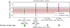 |
Fig. 12. Illustration of H0 estimates resulting from orthogonal paths. The two paths starting with “O” are proper orthogonal paths and can be taken as independent measurements of the Hubble constant. Their weighted mean (red) agrees well with our baseline result despite the latter including all cross-correlations. The shortcuts of the datasets are as defined in the text. The pie charts “fraction of data kept” represent the fraction of statistical power remaining in the path. It is computed as the fraction of the variance of H0 for the given result (in this way multiple datasets with the same constraining power in H0 will be assigned equal percentages). We show the percentages relative to the baseline result (V00). |
The two extensions to O2 considered, O2_V99a and O2_V99, add elements from the “everything” variants (V99a, V99) to improve precision. Both extensions yield H0 values marginally higher than O2 and fully compatible with the respective “everything” variants V99 and V99a. The weighted average H0O1 + O2_V99a = (73.45 ± 0.74) km s−1 Mpc−1 agrees to within < 0.5σ with V99a and features a very similar uncertainty. Finally, the weighted average including the TF relation, H0O1 + O2_V99 = (73.77 ± 0.71) km s−1 Mpc−1, agrees to within 0.4 km s−1 Mpc−1 with V99, with also very similar uncertainty.
Overall these tests confirm both the reliability of the main results as well as the consistent setup of the network. We note that in the case in which the baseline is split into two orthogonal paths we have a mild domination of the uncertainty by the SNe Ia, whereas in the extended cases the uncertainties are relatively balanced.
5.3.2. Paths based on subsets of data
In order to verify the internal consistency of different datasets and methods relevant to determining the Hubble constant, we show below the H0 values obtained for a set of “paths” through the network, each defined by a unique combination of anchors, calibrators, and tracers7. These paths are not all statistically independent by definition, since they might share, for example, a common anchor or a common set of tracer objects. However, we expect the corresponding distribution of H0 values to align at least as well as for independent variables, since we expect the shared data to produce positive, not negative, correlations. In this case, the corresponding test statistics can be regarded as lower bounds on the true values that would be obtained if the full correlation structure were accounted for (i.e., in plain English, if the points sharing the same data are incompatible, it is even worse than points not sharing the same data being incompatible). We find that the Anderson-Darling test cannot reject the null hypothesis of the paths stemming from a Gaussian distribution at 5% confidence level, and we find p = 86.3% for the Shapiro test, both very well within acceptable bounds. We also find no visually strong ( > 2σ) outliers among the paths shown in Fig. 13. Note that since these paths are constructed always using minimal paths through the network, they explicitly do not qualify as "variants" in the sense defined above. We also note that if we were to include the TF case in the generation of these paths, the results worsen quite a bit, to a p ≃ 10% for the Anderson-Darling test and a p ≃ 5% for the Shapiro test, showing once again the high discrepancy of the TF based results within the Distance Network.
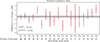 |
Fig. 13. Statistical consistency of various individual paths through the network. These estimates represent a set of paths that are highly correlated, and they often only take a tiny part of the network into account. They are used for a statistical consistency check and should not be interpreted as valid variants in the sense of Sect. 2.4.2. We also show the simple weighted mean of these paths in gray purely for visual purposes, reminding that due to their correlations (and selection effects) it need not necessarily agree with the baseline result. For details on the pie charts, see Fig. 12. |
6. Conclusions and discussion
The Hubble “tension” has persisted for more than a decade and significantly shifted focus among endeavors to precisely measure H0. Before around 2012, the primary motivation for measuring H0 with increasing precision was to provide a strong prior for constraining ΛCDM parameters and understanding dark energy (e.g., Suyu et al. 2012). As the statistical significance of the discrepancy between early- and late-Universe measurements grew, relentless attention was given to systematics of local distance measurements, with an implicit expectation that the tension would be resolved once the responsible systematic error was identified. In other words, there was a non-negligible preference among many to discard direct measurements (even ones with small and detailed uncertainties) based on astronomical techniques in favor of the H0 value derived from the perceived “simple physics” of the early Universe and a specific cosmological model. A narrative of merely two or three direct measurements disagreeing with one extremely precise prediction based on the Planck CMB and flat ΛCDM lent credence to this view, despite a plethora of partially independent measurements painting similar pictures (e.g., Di Valentino et al. 2025, and references therein). A statistically rigorous combination of the available measurements was thus needed to resolve whether any one method might be deemed “bad” or unreliable. The present work provides this long overdue combination supported by expert knowledge from all relevant disciplines, and the results presented discredit the expectation of “unknown unknowns” capable of misleading the direct measurement of the local expansion rate using astronomical techniques.
The Distance Network framework introduced here establishes a reproducible and extensible methodology for synthesizing local distance constraints. Its transparency and modularity allow for the straightforward integration of new data, methods, or calibrators, enabling the community to track the evolution of H0 estimates over time. In addition to the primary distance ladder, the network already incorporates several fully independent paths to H0, including the maser-based anchor, the TRGB-SBF route, and SNe II distances based on astrophysical modeling. These methods rely on distinct physical assumptions and observational systematics, yet they yield results consistent with the primary solution, reinforcing the robustness of the empirical determination. While current uncertainties for these paths are larger, their future competitiveness will depend on targeted improvements in calibration, modeling, and sample size. Promising opportunities include searches for SNe II in SBF or SNe Ia host galaxies, extending TRGB and Cepheid measurements deeper into the Hubble flow using future extremely large ground-based telescopes, denser tiling of NGC 4258 to refine JAGB and TRGB calibrations, and establishing additional anchors via geometric methods (e.g., using population-II pulsating stars calibrated by parallax; e.g., Lengen et al. 2025). Strengthening these independent routes and developing new anchors will be critical for validating and advancing precision cosmology. The approach presented here serves both as a benchmark of current capabilities and as a foundation for future consensus efforts in the determination of H0.
The Distance Network presented in this work provides the most precise direct measurement to date of the Hubble constant, H0 = 73.50 ± 0.81 km s−1 Mpc−1, achieving a relative uncertainty of 1.09%. This value is the result of a comprehensive, covariance-weighted combination of local distance measurements incorporating multiple distance indicators, each rigorously assessed for reliability, consistency, and methodological transparency. By explicitly accounting for shared uncertainties and correlations, the Distance Network formalism surpasses the precision of previous individual or pairwise combinations and reflects a collaborative consensus on data selection, treatment, and analysis strategy.
In constructing the distance network, certain methodological deviations from state-of-the-art analyses were necessary to achieve full covariance treatment across indicators. For example, the use of supernova intercepts for calibration simplifies network integration but does not incorporate the full cross-rung covariance present in datasets such as Pantheon+, as done in Riess et al. (2022b). These trade-offs are explicitly documented to ensure transparency and reproducibility. We are publicly releasing the full Distance Network code upon publication of this paper8.
A central feature of our approach is the construction of a baseline solution exclusively based on top-ranked calibrators and tracers, which were determined by agreement among all authors as representatives of their respective communities. This was complemented by a suite of predefined variants, decided prior to conducting the analysis, that explore the sensitivity of the result to alternative assumptions, datasets, and methodological choices. The resulting spread in H0 values across all variants is significantly smaller than the statistical uncertainty of any individual variant, confirming that no single dataset or technique dominates the result and that the network solution is not driven by any particular methodology or systematic effect. This is also confirmed by investigating routes through the network that are designed to not have any elements in common, leading to results that are highly consistent with the baseline analysis.
Further scrutiny of the systematics affecting Distance Network elements is both necessary and useful for further improvements to H0 accuracy. However, reconciling the Distance Network-based direct H0 measurement with the expectation from ΛCDM would require an extremely unlikely alignment of systematics conspiring to overestimate H0. The diversified portfolio of methods and datasets incorporated into the Distance Network effectively protects against significant bias and demonstrates that the Hubble tension cannot be eliminated by invoking as-yet unidentified systematics in any single method or dataset.
Our result differs by more than 6σ from the value predicted by the ΛCDM model calibrated to Planck CMB observations; by more than 7σ from that calibrated to SPT+ACT CMB measurements, which are given as H0= 67.24 ± 0.35 km s−1 Mpc−1 from Planck+SPT+ACT (Eq. (54) of Camphuis et al. 2025); and by about 5σ from the combination of BBN and DESI BAO constraints, which are H0 = 68.51 ± 0.58 km s−1 Mpc−1 (Tab. V of Abdul Karim et al. 2025). Since the Distance Network provides a conclusive, direct H0 measurement with demonstrated control of systematics, the resulting significant discrepancy retires the aforementioned expectation that identifying a simple systematic could resolve the Hubble constant tension. In this vein, we advocate that the empirically determined value of H0 from the Distance Network be used as a prior in cosmological analyses. This marks a significant shift in perspective: Rather than serving solely to constrain dark energy models, as envisioned a decade ago, the improved accuracy of H0 now exposes a broader inconsistency within the standard cosmological framework and strengthens the case for new physics or a deeper reassessment of early-Universe inferences. The evolving role of H0 has already reshaped our understanding of precision cosmology, and further surprises may lie ahead.
Data availability
The data and analysis code used in this paper are available on Github9. The original version of the code is in IDL; a python version preserving all the main functionality is also available. All the data files needed to run the code as well as corresponding instructions are also available in the repository.
The code is driven by configuration files that determine which data sets are included and other processing parameters. Configuration files corresponding to all the variants presented in Table 4 and many of the other tests are provided. Summary results for each run are provided in the form of text files; in addition, the user has the option of saving the main data, equation coefficients, and covariance matrices in FITS files for more detailed perusal10. It is our intent to update the code and data files with new options and published measurements as they become available.
Acknowledgments
The authors would like to express their sincere gratitude to the ISSI for their hospitality and organization, and especially for a critical role in enabling the scientific discussion and interactions that made this work possible. We are grateful to Fabio Crameri for assistance with visualizations (Figs. 4, 5, 8, and 9). This research has received support from the European Research Council (ERC) under the European Union’s Horizon 2020 research and innovation programme (Grant Agreement No. 947660). RIA is funded by the Swiss National Science Foundation through an Eccellenza Professorial Fellowship (award PCEFP2_194638). The research leading to these results has received funding from the European Research Council (ERC) under the European Union’s Horizon 2020 research and innovation program (project UniverScale, grant agreement 951549). PK acknowledges support from the Polish-French Marie Skłodowska-Curie and Pierre Curie Science Prize awarded by the Foundation for Polish Science. PK acknowledges financial support from the French Agence Nationale de la Recherche (ANR), under grant ANR-23-CE31-0009-01 (Unlock-pfactor). AB thanks the funding from the Anusandhan National Research Foundation (ANRF), Government of India, under the Prime Minister Early Career Research Grant scheme (ANRF/ECRG/2024/000675/PMS). LV and HGM acknowledge support of Spanish MINECO under project PID2022-141125NB-I00 MCIN/AEI, and Center of Excellence Maria de Maeztu Grant CEX2024-001451-M funded by MICIU/AEI/10.13039/501100011033. LG acknowledges financial support from AGAUR, CSIC, MCIN and AEI 10.13039/501100011033 under projects PID2023-151307NB-I00, PIE 20215AT016, CEX2020-001058-M, ILINK23001, COOPB2304, and 2021-SGR-01270. EDV is supported by a Royal Society Dorothy Hodgkin Research Fellowship. NS acknowledges support from the Excellence Cluster ORIGINS which is funded by the Deutsche Forschungsgemeinschaft (DFG, German Research Foundation) under Germany’s Excellence Strategy – EXC-2094 – 390783311, as well as the funding through a Fraunhofer-Schwarzschild Fellowship at the LMU. MC acknowledges support from ASI-INAF grant no. 2024-10-HH.0 (WP8420), the ESO Scientific Visitor Programme, and INAF GO-grant no. 12/2024. JJ acknowledges support from NASA/STScI through grants HST-GO-17436 and JWST-GO-5989. SC and GA acknowledge support from NASA/STScI through grants HST-GO-17098, JWST-GO-1685 and JWST-GO-2875. This article is based upon work from COST Action CA21136 “Addressing observational tensions in cosmology with systematics and fundamental physics” (CosmoVerse), supported by COST (European Cooperation in Science and Technology). This research was supported by the International Space Science Institute (ISSI) in Bern/Beijing through ISSI/ISSI-BJ International Team project ID #24-603 – “EXPANDING Universe” (EXploiting Precision AstroNomical Distance INdicators in the Gaia Universe). This research was supported by the Munich Institute for Astro-, Particle and BioPhysics (MIAPbP) which is funded by the Deutsche Forschungsgemeinschaft (DFG, German Research Foundation) under Germany’s Excellence Strategy – EXC-2094 – 390783311. Statement of individuals’ relevant expertise: Casertano–SN Ia, Cepheids, TRGB, network analysis; Anand–TRGB, HST, JWST, TF; Anderson–Cepheids, TRGB, star clusters, systematics of stellar standard candles; Beaton–TRGB, AGB, stellar populations; Bhardwaj–Cepheids, Miras, metallicity, clusters; Blakeslee–SBF; Boubel–TF relation; Breuval–Cepheids, metallicity, clusters; Brout–SN Ia, Pantheons+; Cantiello–SBF; Cruz Reyes–Cepheids, clusters; Csörnyei–SN II; de Jaeger–SN II; Dhawan–SN Ia, BayesSN; Di Valentino–cosmological analyses; Galbany–SN Ia, near-IR, SNooPy, SN II.; Gil-Marín–cosmological analyses; Graczyk–DEBs; Huang–Miras; Jensen–SBF; Kervella–Cepheids, metallicity, DEBs; Leibundgut–SN Ia, SN II; Lengen–Clusters; Li–JAGB, TRGB; Macri–Cepheids, Miras; Özülker–cosmological analyses; Pesce–Masers, Radio observations; Riess–SN Ia, Cepheids, HST, JWST; Romaniello–Cepheids, metallicity; Said-TF, FP, peculiar velocities; Schöneberg–cosmological analyses, BAO+BBN, CMB, H0 tension; Scolnic–SN Ia, Pantheon +; Sicignano–Cepheids; Skowron–DEBs, reddening maps; Uddin–SN Ia cosmology, Hubble constant analysis, CSP; Verde–cosmological analyses; Nota–Organizer.
References
- Abdul Karim, M., Aguilar, S., Ahlen, S., et al. 2025, Phys. Rev. D, 112, 083515 [Google Scholar]
- Adams, C., & Blake, C. 2020, MNRAS, 494, 3275 [NASA ADS] [CrossRef] [Google Scholar]
- Aitken, A. C. 1935, Proc. Royal Soc. Edinburgh, 55, 42 [Google Scholar]
- Anand, G. S., Rizzi, L., Tully, R. B., et al. 2021, AJ, 162, 80 [CrossRef] [Google Scholar]
- Anand, G. S., Tully, R. B., Rizzi, L., Riess, A. G., & Yuan, W. 2022, ApJ, 932, 15 [NASA ADS] [CrossRef] [Google Scholar]
- Anand, G. S., Riess, A. G., Yuan, W., et al. 2024a, ApJ, 966, 89 [NASA ADS] [CrossRef] [Google Scholar]
- Anand, G. S., Tully, R. B., Cohen, Y., et al. 2024b, ApJ, 973, 83 [Google Scholar]
- Anand, G. S., Tully, R. B., Cohen, Y., et al. 2025, ApJ, 982, 26 [Google Scholar]
- Anderson, R. I. 2019, A&A, 631, A165 [NASA ADS] [CrossRef] [EDP Sciences] [Google Scholar]
- Anderson, R. I. 2022, A&A, 658, A148 [NASA ADS] [CrossRef] [EDP Sciences] [Google Scholar]
- Anderson, R. I., & Riess, A. G. 2018, ApJ, 861, 36 [NASA ADS] [CrossRef] [Google Scholar]
- Anderson, J. P., Contreras, C., Stritzinger, M. D., et al. 2024a, A&A, 692, A95 [NASA ADS] [CrossRef] [EDP Sciences] [Google Scholar]
- Anderson, R. I., Koblischke, N. W., & Eyer, L. 2024b, ApJ, 963, L43 [NASA ADS] [CrossRef] [Google Scholar]
- Argon, A. L., Greenhill, L. J., Reid, M. J., Moran, J. M., & Humphreys, E. M. L. 2007, ApJ, 659, 1040 [Google Scholar]
- Baltay, C., Rabinowitz, D., Hadjiyska, E., et al. 2013, PASP, 125, 683 [Google Scholar]
- Beaton, R. L., Bono, G., Braga, V. F., et al. 2018, Space Sci. Rev., 214, 113 [NASA ADS] [CrossRef] [Google Scholar]
- Bhardwaj, A., Rejkuba, M., de Grijs, R., et al. 2021, ApJ, 909, 200 [NASA ADS] [CrossRef] [Google Scholar]
- Bhardwaj, A., Riess, A. G., Catanzaro, G., et al. 2023, ApJ, 955, L13 [NASA ADS] [CrossRef] [Google Scholar]
- Bhardwaj, A., Ripepi, V., Testa, V., et al. 2024, A&A, 683, A234 [NASA ADS] [CrossRef] [EDP Sciences] [Google Scholar]
- Bhardwaj, A., Matsunaga, N., Huang, C. D., Riess, A. G., & Rejkuba, M. 2025, ApJ, 990, 63 [Google Scholar]
- Blakeslee, J. P., Jensen, J. B., Ma, C.-P., Milne, P. A., & Greene, J. E. 2021, ApJ, 911, 65 [NASA ADS] [CrossRef] [Google Scholar]
- Boubel, P., Colless, M., Said, K., & Staveley-Smith, L. 2024a, MNRAS, 533, 1550 [Google Scholar]
- Boubel, P., Colless, M., Said, K., & Staveley-Smith, L. 2024b, MNRAS, 531, 84 [Google Scholar]
- Braatz, J., Greenhill, L., Reid, M., et al. 2007, IAU Symp., 242, 399 [Google Scholar]
- Braatz, J. A., Reid, M. J., Humphreys, E. M. L., et al. 2010, ApJ, 718, 657 [NASA ADS] [CrossRef] [Google Scholar]
- Braatz, J., Condon, J., Constantin, A., et al. 2015, IAU Gen. Assemb., 29, 2255730 [Google Scholar]
- Breuval, L., Kervella, P., Anderson, R. I., et al. 2020, A&A, 643, A115 [EDP Sciences] [Google Scholar]
- Breuval, L., Riess, A. G., Kervella, P., Anderson, R. I., & Romaniello, M. 2022, ApJ, 939, 89 [NASA ADS] [CrossRef] [Google Scholar]
- Breuval, L., Riess, A. G., Casertano, S., et al. 2024, ApJ, 973, 30 [Google Scholar]
- Breuval, L., Anand, G. S., Anderson, R. I., et al. 2025, ApJ, 994, 111 [Google Scholar]
- Brout, D., Scolnic, D., Popovic, B., et al. 2022a, ApJ, 938, 110 [NASA ADS] [CrossRef] [Google Scholar]
- Brout, D., Taylor, G., Scolnic, D., et al. 2022b, ApJ, 938, 111 [NASA ADS] [CrossRef] [Google Scholar]
- Burns, C. R., Stritzinger, M., Phillips, M. M., et al. 2011, AJ, 141, 19 [Google Scholar]
- Calcino, J., & Davis, T. 2017, JCAP, 2017, 038 [Google Scholar]
- Camphuis, E., Quan, W., Balkenhol, L., et al. 2025, ArXiv e-prints [arXiv:2506.20707] [Google Scholar]
- Cantiello, M., & Blakeslee, J. P. 2023, ArXiv e-prints [arXiv:2307.03116] [Google Scholar]
- Cappellari, M. 2023, MNRAS, 526, 3273 [NASA ADS] [CrossRef] [Google Scholar]
- Carr, A., Davis, T. M., Scolnic, D., et al. 2022, PASA, 39, e046 [NASA ADS] [CrossRef] [Google Scholar]
- Carrick, J., Turnbull, S. J., Lavaux, G., & Hudson, M. J. 2015, MNRAS, 450, 317 [Google Scholar]
- Casertano, S., Riess, A. G., Anderson, J., et al. 2016, ApJ, 825, 11 [Google Scholar]
- Ciardullo, R. 2006, in Planetary Nebulae Beyond the Milky Way, eds. L. Stanghellini, J. R. Walsh, & N. G. Douglas, 79 [Google Scholar]
- Claussen, M. J., Reid, M. J., Schneps, M. H., et al. 1988, IAU Symp., 129, 231 [Google Scholar]
- Cruz Reyes, M., & Anderson, R. I. 2023, A&A, 672, A85 [NASA ADS] [CrossRef] [EDP Sciences] [Google Scholar]
- Csörnyei, G., Anderson, R. I., Vogl, C., et al. 2023a, A&A, 678, A44 [NASA ADS] [CrossRef] [EDP Sciences] [Google Scholar]
- Csörnyei, G., Vogl, C., Taubenberger, S., et al. 2023b, A&A, 672, A129 [NASA ADS] [CrossRef] [EDP Sciences] [Google Scholar]
- D’Andrea, C. B., Sako, M., Dilday, B., et al. 2010, ApJ, 708, 661 [Google Scholar]
- Davis, T. M., Hui, L., Frieman, J. A., et al. 2011, ApJ, 741, 67 [NASA ADS] [CrossRef] [Google Scholar]
- Davis, T. M., Hinton, S. R., Howlett, C., & Calcino, J. 2019, MNRAS, 490, 2948 [NASA ADS] [CrossRef] [Google Scholar]
- de Grijs, R. 2013, IAU Symp., 289, 351 [Google Scholar]
- de Jaeger, T., & Galbany, L. 2024, in The Hubble Constant Tension, eds. E. Dillon, & B. Di Valentino, 177 [Google Scholar]
- de Jaeger, T., Galbany, L., Filippenko, A. V., et al. 2017a, MNRAS, 472, 4233 [NASA ADS] [CrossRef] [Google Scholar]
- de Jaeger, T., González-Gaitán, S., Hamuy, M., et al. 2017b, ApJ, 835, 166 [NASA ADS] [CrossRef] [Google Scholar]
- de Jaeger, T., Zheng, W., Stahl, B. E., et al. 2019, MNRAS, 490, 2799 [NASA ADS] [CrossRef] [Google Scholar]
- de Jaeger, T., Galbany, L., González-Gaitán, S., et al. 2020a, MNRAS, 495, 4860 [NASA ADS] [CrossRef] [Google Scholar]
- de Jaeger, T., Stahl, B. E., Zheng, W., et al. 2020b, MNRAS, 496, 3402 [NASA ADS] [CrossRef] [Google Scholar]
- de Jaeger, T., Galbany, L., Riess, A. G., et al. 2022, MNRAS, 514, 4620 [NASA ADS] [CrossRef] [Google Scholar]
- DESI Collaboration (Adame, A. G., et al.) 2024, AJ, 168, 58 [NASA ADS] [CrossRef] [Google Scholar]
- Dessart, L., & Hillier, D. J. 2005, A&A, 439, 671 [NASA ADS] [CrossRef] [EDP Sciences] [Google Scholar]
- Dey, A., Schlegel, D. J., Lang, D., et al. 2019, AJ, 157, 168 [Google Scholar]
- Dhawan, S., Goobar, A., Johansson, J., et al. 2022, ApJ, 934, 185 [NASA ADS] [CrossRef] [Google Scholar]
- Dhawan, S., Thorp, S., Mandel, K. S., et al. 2023, MNRAS, 524, 235 [Google Scholar]
- Di Valentino, E., Mena, O., Pan, S., et al. 2021, Class. Quant. Grav., 38, 153001 [NASA ADS] [CrossRef] [Google Scholar]
- Di Valentino, E., Said, J. L., Riess, A., et al. 2025, Phys. Dark Univ., 49, 101965 [Google Scholar]
- Djorgovski, S., & Davis, M. 1987, ApJ, 313, 59 [Google Scholar]
- Dressler, A., Lynden-Bell, D., Burstein, D., et al. 1987, ApJ, 313, 42 [Google Scholar]
- Fitzpatrick, E. L., & Massa, D. 2007, ApJ, 663, 320 [Google Scholar]
- Folatelli, G., Morrell, N., Phillips, M. M., et al. 2013, ApJ, 773, 53 [Google Scholar]
- Freedman, W. 2014, CHP-II: The Carnegie Hubble Program to Measure Ho to 3% Using Population II, HST Proposal ID 13691. Cycle 22 [Google Scholar]
- Freedman, W. L. 2018, An Independent Determination of the Hubble Constant, HST Proposal Cycle 26, ID. # 15642 [Google Scholar]
- Freedman, W. L., & Madore, B. F. 2010, ARA&A, 48, 673 [Google Scholar]
- Freedman, W. L., Madore, B. F., Gibson, B. K., et al. 2001, ApJ, 553, 47 [Google Scholar]
- Freedman, W. L., Madore, B. F., Hatt, D., et al. 2019, ApJ, 882, 34 [Google Scholar]
- Freedman, W. L., Madore, B. F., Hoyt, T., et al. 2021, Answering the Most Important Problem in Cosmology Today: Is the Tension in the Hubble Constant Real?, JWST Proposal. Cycle 1, ID. 1995 [Google Scholar]
- Freedman, W. L., Madore, B. F., Hoyt, T. J., et al. 2025, ApJ, 985, 203 [Google Scholar]
- Gaia Collaboration (Prusti, T., et al.) 2016, A&A, 595, A1 [NASA ADS] [CrossRef] [EDP Sciences] [Google Scholar]
- Gaia Collaboration (Brown, A. G. A., et al.) 2021, A&A, 649, A1 [NASA ADS] [CrossRef] [EDP Sciences] [Google Scholar]
- Galbany, L., de Jaeger, T., Riess, A. G., et al. 2023, A&A, 679, A95 [NASA ADS] [CrossRef] [EDP Sciences] [Google Scholar]
- Gallenne, A., Pietrzyński, G., Graczyk, D., et al. 2019, A&A, 632, A31 [EDP Sciences] [Google Scholar]
- Gao, F., Braatz, J. A., Reid, M. J., et al. 2016, ApJ, 817, 128 [NASA ADS] [CrossRef] [Google Scholar]
- Garnavich, P., Wood, C. M., Milne, P., et al. 2023, ApJ, 953, 35 [NASA ADS] [CrossRef] [Google Scholar]
- Gommers, R., Virtanen, P., Haberland, M., et al. 2025, https://doi.org/10.5281/zenodo.595738 [Google Scholar]
- Graczyk, D., Pietrzyński, G., Thompson, I. B., et al. 2018, ApJ, 860, 1 [NASA ADS] [CrossRef] [Google Scholar]
- Graczyk, D., Pietrzyński, G., Thompson, I. B., et al. 2020, ApJ, 904, 13 [Google Scholar]
- Gratton, S., & Challinor, A. 2020, MNRAS, 499, 3410 [Google Scholar]
- Graziani, R., Courtois, H. M., Lavaux, G., et al. 2019, MNRAS, 488, 5438 [NASA ADS] [CrossRef] [Google Scholar]
- Greenhill, L. J., Jiang, D. R., Moran, J. M., et al. 1995, ApJ, 440, 619 [Google Scholar]
- Hamuy, M., & Pinto, P. A. 2002, ApJ, 566, L63 [NASA ADS] [CrossRef] [Google Scholar]
- Hamuy, M., Folatelli, G., Morrell, N. I., et al. 2006, PASP, 118, 2 [NASA ADS] [CrossRef] [Google Scholar]
- Haschke, R., Grebel, E. K., & Duffau, S. 2011, AJ, 141, 158 [NASA ADS] [Google Scholar]
- Herrnstein, J. R., Moran, J. M., Greenhill, L. J., et al. 1999, Nature, 400, 539 [NASA ADS] [CrossRef] [Google Scholar]
- Hinton, S., & Brout, D. 2020, J. Open Source Softw., 5, 2122 [NASA ADS] [CrossRef] [Google Scholar]
- Hoyt, T. J., Beaton, R. L., Freedman, W. L., et al. 2021, ApJ, 915, 34 [NASA ADS] [CrossRef] [Google Scholar]
- Hoyt, T. J., Jang, I. S., Freedman, W. L., et al. 2025, ArXiv e-prints [arXiv:2503.11769] [Google Scholar]
- Hsiao, E. Y., Phillips, M. M., Marion, G. H., et al. 2019, PASP, 131, 014002 [NASA ADS] [CrossRef] [Google Scholar]
- Huang, C. D., Riess, A. G., Hoffmann, S. L., et al. 2018, ApJ, 857, 67 [NASA ADS] [CrossRef] [Google Scholar]
- Huang, C. D., Riess, A. G., Yuan, W., et al. 2020, ApJ, 889, 5 [Google Scholar]
- Huang, C. D., Yuan, W., Riess, A. G., et al. 2024, ApJ, 963, 83 [Google Scholar]
- Humphreys, E. M. L., Reid, M. J., Greenhill, L. J., Moran, J. M., & Argon, A. L. 2008, ApJ, 672, 800 [NASA ADS] [CrossRef] [Google Scholar]
- Humphreys, E. M. L., Reid, M. J., Moran, J. M., Greenhill, L. J., & Argon, A. L. 2013, ApJ, 775, 13 [Google Scholar]
- Jacoby, G. H., Branch, D., Ciardullo, R., et al. 1992, PASP, 104, 599 [Google Scholar]
- Jang, I. S., Hoyt, T. J., Beaton, R. L., et al. 2021, ApJ, 906, 125 [NASA ADS] [CrossRef] [Google Scholar]
- Jang, I. S., & Lee, M. G. 2017, ApJ, 836, 74 [NASA ADS] [CrossRef] [Google Scholar]
- Jensen, J. B., Blakeslee, J. P., Gibson, Z., et al. 2015, ApJ, 808, 91 [Google Scholar]
- Jensen, J. B., Blakeslee, J. P., Ma, C.-P., et al. 2021, ApJS, 255, 21 [Google Scholar]
- Jensen, J. B., Blakeslee, J. P., Cantiello, M., et al. 2025, ApJ, 987, 87 [Google Scholar]
- Jha, S., Garnavich, P. M., Kirshner, R. P., et al. 1999, ApJS, 125, 73 [CrossRef] [Google Scholar]
- Jones, D. O., Kenworthy, W. D., Dai, M., et al. 2023, ApJ, 951, 22 [NASA ADS] [CrossRef] [Google Scholar]
- Jorgensen, I., Franx, M., & Kjaergaard, P. 1995, MNRAS, 276, 1341 [NASA ADS] [Google Scholar]
- Kamionkowski, M., & Riess, A. G. 2023, Ann. Rev. Nucl. Part. Sci., 73, 153 [NASA ADS] [CrossRef] [Google Scholar]
- Kenworthy, W. D., Jones, D. O., Dai, M., et al. 2021, ApJ, 923, 265 [NASA ADS] [CrossRef] [Google Scholar]
- Kenworthy, W. D., Riess, A. G., Scolnic, D., et al. 2022, ApJ, 935, 83 [NASA ADS] [CrossRef] [Google Scholar]
- Kerzendorf, W. E., & Sim, S. A. 2014, MNRAS, 440, 387 [NASA ADS] [CrossRef] [Google Scholar]
- Khan, S., Anderson, R. I., Miglio, A., Mosser, B., & Elsworth, Y. P. 2023, A&A, 680, A105 [NASA ADS] [CrossRef] [EDP Sciences] [Google Scholar]
- Khan, S., Anderson, R. I., Ekström, S., Georgy, C., & Breuval, L. 2025, A&A, 702, A235 [NASA ADS] [CrossRef] [EDP Sciences] [Google Scholar]
- Kirshner, R. P., & Kwan, J. 1974, ApJ, 193, 27 [NASA ADS] [CrossRef] [Google Scholar]
- Kourkchi, E., Tully, R. B., Eftekharzadeh, S., et al. 2020, ApJ, 902, 145 [NASA ADS] [CrossRef] [Google Scholar]
- Krisciunas, K., Contreras, C., Burns, C. R., et al. 2017, AJ, 154, 211 [NASA ADS] [CrossRef] [Google Scholar]
- Kuo, C. Y., Braatz, J. A., Reid, M. J., et al. 2013, ApJ, 767, 155 [NASA ADS] [CrossRef] [Google Scholar]
- Kuo, C. Y., Braatz, J. A., Lo, K. Y., et al. 2015, ApJ, 800, 26 [NASA ADS] [CrossRef] [Google Scholar]
- Kuo, C. Y., Hsiang, J. Y., Chung, H. H., et al. 2020, ApJ, 892, 18 [Google Scholar]
- Laney, C. D., Joner, M. D., & Pietrzyński, G. 2012, MNRAS, 419, 1637 [Google Scholar]
- Lapack Contributors 2021, Astrophysics Source Code Library [record ascl:2104.020] [Google Scholar]
- Leavitt, H. S., & Pickering, E. C. 1912, Harvard College Observatory Circular, 173, 1 [Google Scholar]
- Lee, A. J., Freedman, W. L., Madore, B. F., et al. 2025, ApJ, 985, 182 [Google Scholar]
- Lengen, B., Anderson, R. I., Cruz Reyes, M., & Viviani, G. 2025, ArXiv e-prints [arXiv:2509.16331] [Google Scholar]
- Li, S., Anand, G. S., Riess, A. G., et al. 2024a, ApJ, 976, 177 [Google Scholar]
- Li, S., Riess, A. G., Casertano, S., et al. 2024b, ApJ, 966, 20 [NASA ADS] [CrossRef] [Google Scholar]
- Li, S., Riess, A. G., Anand, G. S., et al. 2025a, ArXiv e-prints [arXiv:2504.08921] [Google Scholar]
- Li, S., Riess, A. G., Scolnic, D., Casertano, S., & Anand, G. S. 2025b, ApJ, 988, 97 [Google Scholar]
- Lilow, R., & Nusser, A. 2021, MNRAS, 507, 1557 [NASA ADS] [CrossRef] [Google Scholar]
- Lindegren, L., Bastian, U., Biermann, M., et al. 2021a, A&A, 649, A4 [EDP Sciences] [Google Scholar]
- Lindegren, L., Klioner, S. A., Hernández, J., et al. 2021b, A&A, 649, A2 [EDP Sciences] [Google Scholar]
- Magnus, E., Groenewegen, M. A. T., Girardi, L., et al. 2024, A&A, 691, A350 [NASA ADS] [CrossRef] [EDP Sciences] [Google Scholar]
- Marion, G. H., Brown, P. J., Vinkó, J., et al. 2016, ApJ, 820, 92 [NASA ADS] [CrossRef] [Google Scholar]
- McQuinn, K. B. W., Boyer, M., Skillman, E. D., & Dolphin, A. E. 2019, ApJ, 880, 63 [Google Scholar]
- Mermilliod, J. C., Mermilliod, M., & Hauck, B. 1997, A&AS, 124, 349 [NASA ADS] [CrossRef] [EDP Sciences] [Google Scholar]
- Miyoshi, M., Moran, J., Herrnstein, J., et al. 1995, Nature, 373, 127 [NASA ADS] [CrossRef] [Google Scholar]
- Morrell, N., Phillips, M. M., Folatelli, G., et al. 2024, ApJ, 967, 20 [Google Scholar]
- Munari, U., & Zwitter, T. 1997, A&A, 318, 269 [NASA ADS] [Google Scholar]
- Murakami, Y. S., Riess, A. G., Stahl, B. E., et al. 2023, JCAP, 2023, 046 [CrossRef] [Google Scholar]
- Nugent, P., Sullivan, M., Ellis, R., et al. 2006, ApJ, 645, 841 [CrossRef] [Google Scholar]
- Parada, J., Heyl, J., Richer, H., Ripoche, P., & Rousseau-Nepton, L. 2021, MNRAS, 501, 933 [Google Scholar]
- Parada, J., Heyl, J., Richer, H., Ripoche, P., & Rousseau-Nepton, L. 2023, MNRAS, 522, 195 [NASA ADS] [CrossRef] [Google Scholar]
- Penrose, R. 1956, Math. Proc. Camb. Philos. Soc., 52, 17 [Google Scholar]
- Pesce, D. W., Braatz, J. A., Reid, M. J., et al. 2020a, ApJ, 890, 118 [NASA ADS] [CrossRef] [Google Scholar]
- Pesce, D. W., Braatz, J. A., Reid, M. J., et al. 2020b, ApJ, 891, L1 [Google Scholar]
- Peterson, E., Kenworthy, W., Scolnic, D., et al. 2023, Am. Astron. Soc. Meet. Abstr., 241, 424.08 [Google Scholar]
- Phillips, M. M., Contreras, C., Hsiao, E. Y., et al. 2019, PASP, 131, 014001 [Google Scholar]
- Pietrzyński, G., Thompson, I. B., Graczyk, D., et al. 2009, ApJ, 697, 862 [CrossRef] [Google Scholar]
- Pietrzyński, G., Graczyk, D., Gallenne, A., et al. 2019, Nature, 567, 200 [Google Scholar]
- Popovic, B., Brout, D., Kessler, R., Scolnic, D., & Lu, L. 2021, ApJ, 913, 49 [NASA ADS] [CrossRef] [Google Scholar]
- Popovic, B., Brout, D., Kessler, R., & Scolnic, D. 2023, ApJ, 945, 84 [NASA ADS] [CrossRef] [Google Scholar]
- Reid, M. J., Braatz, J. A., Condon, J. J., et al. 2009, ApJ, 695, 287 [Google Scholar]
- Reid, M. J., Braatz, J. A., Condon, J. J., et al. 2013, ApJ, 767, 154 [NASA ADS] [CrossRef] [Google Scholar]
- Reid, M. J., Pesce, D. W., & Riess, A. G. 2019, ApJ, 886, L27 [Google Scholar]
- Richmond, M. W., & Smith, H. A. 2012, JAAVSO, 40, 872 [Google Scholar]
- Riess, A. 2002, Determining Hubble’s Constant from Observations of Cepheids in the Host Galaxy of SN Ia 1994ae, HST Proposal ID 9351, Cycle 11 [Google Scholar]
- Riess, A. 2005, Cepheid Calibrations of the Luminosity of Two Reliable Type Ia Supernovae and a Re-determination of the Hubble Constant, HST Proposal ID 10497, Cycle 14 [Google Scholar]
- Riess, A. 2006, SHOES-Supernovae, H0, for the Equation of State of Dark energy, HST Proposal ID 10802. Cycle 15 [Google Scholar]
- Riess, A. G., Kirshner, R. P., Schmidt, B. P., et al. 1999, AJ, 117, 707 [Google Scholar]
- Riess, A. G., Li, W., Stetson, P. B., et al. 2005, ApJ, 627, 579 [Google Scholar]
- Riess, A. G., Strolger, L.-G., Casertano, S., et al. 2007, ApJ, 659, 98 [NASA ADS] [CrossRef] [Google Scholar]
- Riess, A. G., Macri, L., Casertano, S., et al. 2009a, ApJ, 699, 539 [Google Scholar]
- Riess, A. G., Macri, L., Li, W., et al. 2009b, ApJS, 183, 109 [NASA ADS] [CrossRef] [Google Scholar]
- Riess, A. G., Casertano, S., Anderson, J., MacKenty, J., & Filippenko, A. V. 2014, ApJ, 785, 161 [Google Scholar]
- Riess, A. G., Macri, L. M., Hoffmann, S. L., et al. 2016, ApJ, 826, 56 [Google Scholar]
- Riess, A. G., Casertano, S., Yuan, W., et al. 2018, ApJ, 855, 136 [Google Scholar]
- Riess, A. G., Casertano, S., Yuan, W., Macri, L. M., & Scolnic, D. 2019, ApJ, 876, 85 [Google Scholar]
- Riess, A. G., Casertano, S., Yuan, W., et al. 2021, ApJ, 908, L6 [NASA ADS] [CrossRef] [Google Scholar]
- Riess, A. G., Breuval, L., Yuan, W., et al. 2022a, ApJ, 938, 36 [NASA ADS] [CrossRef] [Google Scholar]
- Riess, A. G., Yuan, W., Macri, L. M., et al. 2022b, ApJ, 934, L7 [NASA ADS] [CrossRef] [Google Scholar]
- Riess, A. G., Anand, G. S., Yuan, W., et al. 2023, ApJ, 956, L18 [NASA ADS] [CrossRef] [Google Scholar]
- Riess, A. G., Scolnic, D., Anand, G. S., et al. 2024, ApJ, 977, 120 [NASA ADS] [CrossRef] [Google Scholar]
- Riess, A. G., Li, S., Anand, G. S., et al. 2025, ApJ, 992, L34 [Google Scholar]
- Ripoche, P., Heyl, J., Parada, J., & Richer, H. 2020, MNRAS, 495, 2858 [NASA ADS] [CrossRef] [Google Scholar]
- Rizzi, L., Tully, R. B., Makarov, D., et al. 2007, ApJ, 661, 815 [Google Scholar]
- Romaniello, M., Riess, A., Mancino, S., et al. 2022, A&A, 658, A29 [NASA ADS] [CrossRef] [EDP Sciences] [Google Scholar]
- Roy, R., Kumar, B., Benetti, S., et al. 2011, ApJ, 736, 76 [NASA ADS] [CrossRef] [Google Scholar]
- Sahu, D. K., Anupama, G. C., Srividya, S., & Muneer, S. 2006, MNRAS, 372, 1315 [Google Scholar]
- Said, K., Colless, M., Magoulas, C., Lucey, J. R., & Hudson, M. J. 2020, MNRAS, 497, 1275 [NASA ADS] [CrossRef] [Google Scholar]
- Said, K., Howlett, C., Davis, T., et al. 2025, MNRAS, 539, 3627 [Google Scholar]
- Sandage, A., Tammann, G. A., Saha, A., et al. 2006, ApJ, 653, 843 [Google Scholar]
- Schlafly, E. F., & Finkbeiner, D. P. 2011, ApJ, 737, 103 [Google Scholar]
- Schlegel, D. J., Finkbeiner, D. P., & Davis, M. 1998, ApJ, 500, 525 [Google Scholar]
- Schmidt, B. P., Kirshner, R. P., Eastman, R. G., et al. 1994, ApJ, 432, 42 [NASA ADS] [CrossRef] [Google Scholar]
- Scolnic, D., Boubel, P., Byrne, J., Riess, A. G., & Anand, G. S. 2024, ArXiv e-prints [arXiv:2412.08449] [Google Scholar]
- Scolnic, D., Brout, D., Carr, A., et al. 2022, ApJ, 938, 113 [NASA ADS] [CrossRef] [Google Scholar]
- Scolnic, D., Riess, A. G., Murakami, Y. S., et al. 2025, ApJ, 979, L9 [Google Scholar]
- Serenelli, A., Weiss, A., Cassisi, S., Salaris, M., & Pietrinferni, A. 2017, A&A, 606, A33 [NASA ADS] [CrossRef] [EDP Sciences] [Google Scholar]
- Shah, P., Lemos, P., & Lahav, O. 2021, A&ARv, 29, 9 [NASA ADS] [CrossRef] [Google Scholar]
- Smartt, S. J., Valenti, S., Fraser, M., et al. 2015, A&A, 579, A40 [NASA ADS] [CrossRef] [EDP Sciences] [Google Scholar]
- Stahl, B. E., Zheng, W., de Jaeger, T., et al. 2019, MNRAS, 490, 3882 [NASA ADS] [CrossRef] [Google Scholar]
- Strauss, M. A., & Willick, J. A. 1995, Phys. Rep., 261, 271 [NASA ADS] [CrossRef] [Google Scholar]
- Suyu, S. H., Treu, T., Blandford, R. D., et al. 2012, ArXiv e-prints [arXiv:1202.4459] [Google Scholar]
- Szalai, T., Vinkó, J., Könyves-Tóth, R., et al. 2019, ApJ, 876, 19 [Google Scholar]
- Taylor, G., Lidman, C., Tucker, B. E., et al. 2021, MNRAS, 504, 4111 [NASA ADS] [CrossRef] [Google Scholar]
- Tdcosmo Collaboration (Birrer, S., et al.) 2025, A&A, 704, A63 [Google Scholar]
- Teja, R. S., Singh, A., Sahu, D. K., et al. 2022, ApJ, 930, 34 [NASA ADS] [CrossRef] [Google Scholar]
- Tonry, J., & Schneider, D. P. 1988, AJ, 96, 807 [Google Scholar]
- Trentin, E., Catanzaro, G., Ripepi, V., et al. 2024, A&A, 690, A246 [NASA ADS] [CrossRef] [EDP Sciences] [Google Scholar]
- Tully, R. B., & Fisher, J. R. 1977, A&A, 54, 661 [NASA ADS] [Google Scholar]
- Tully, R. B., Rizzi, L., Shaya, E. J., et al. 2009, AJ, 138, 323 [NASA ADS] [CrossRef] [Google Scholar]
- Turner, R. J., Blake, C., & Ruggeri, R. 2023, MNRAS, 518, 2436 [Google Scholar]
- Udalski, A., Szymański, M. K., & Szymański, G. 2015, Acta Astron., 65, 1 [NASA ADS] [Google Scholar]
- Uddin, S. A., Burns, C. R., Phillips, M. M., et al. 2024, ApJ, 970, 72 [Google Scholar]
- Valdes, F., Gupta, R., Rose, J. A., Singh, H. P., & Bell, D. J. 2004, ApJS, 152, 251 [Google Scholar]
- Verde, L., Treu, T., & Riess, A. G. 2019, Nat. Astron., 3, 891 [Google Scholar]
- Verde, L., Schöneberg, N., & Gil-Marín, H. 2024, ARA&A, 62, 287 [Google Scholar]
- Vogl, C., Sim, S. A., Noebauer, U. M., Kerzendorf, W. E., & Hillebrandt, W. 2019, A&A, 621, A29 [NASA ADS] [CrossRef] [EDP Sciences] [Google Scholar]
- Vogl, C., Kerzendorf, W. E., Sim, S. A., et al. 2020, A&A, 633, A88 [NASA ADS] [CrossRef] [EDP Sciences] [Google Scholar]
- Vogl, C., Taubenberger, S., Csörnyei, G., et al. 2025, A&A, 702, A41 [NASA ADS] [CrossRef] [EDP Sciences] [Google Scholar]
- Wang, C., Yuan, H., & Huang, Y. 2022, AJ, 163, 149 [NASA ADS] [CrossRef] [Google Scholar]
- Wang, H., Xu, Y., Lin, Z., et al. 2024, AJ, 168, 34 [NASA ADS] [CrossRef] [Google Scholar]
- Wilson, R. E., & Devinney, E. J. 1971, ApJ, 166, 605 [Google Scholar]
- Yuan, W., Macri, L. M., Riess, A. G., et al. 2022, ApJ, 940, 64 [NASA ADS] [CrossRef] [Google Scholar]
- Zgirski, B., Pietrzyński, G., Gieren, W., et al. 2021, ApJ, 916, 19 [NASA ADS] [CrossRef] [Google Scholar]
- Zheng, W., Dessart, L., Filippenko, A. V., et al. 2025, ApJ, 988, 61 [Google Scholar]
Though the overall acceptance rate was high (> 90%), several invitees were unable to attend or declined participation in the workshop. Following the inclusive spirit of the workshop, opportunities for remote participation via Zoom and asynchronous participation by e-mail were offered in such cases. Several members and leaders of the CCHP group were invited but declined to participate; however, their published results are included in the analysis whenever they satisfy the ground rules for inclusion.
We make conventional assumptions common to distance ladders: that the cosmological principle holds so that we do not live in a special place (i.e., there is no intrinsic difference in objects solely based on their separation from us); that evolution over short lookback times, of order a few hundred Myr, is negligible; and that the expansion history for z < 0.15 can be approximated with an expansion of a few kinematic terms, namely H0, q0, and j0.
Note that the current version only uses TRGB measurements for the calibration of the SBF method, in accordance with the most recent publication (Jensen et al. 2025); in future iterations we intend to allow for arbitrary primary distance indicators for the calibration.
This is a slightly simplified description of the uncertainties, as it accounts for most, but not all, covariances in the data. However, it is a useful guide to the properties of residuals, as long as the formal χ2 is consistent with the statistics of the system.
In principle, more orthogonal paths could be formulated (e.g., by separating out specific one-step methods), but such combinations of paths are typically not balanced in their constraining power.
In practice we construct these paths as minimal combinations, except where this might lead to ambiguities. First we use each of the possible calibrator sets (e.g., Cepheids measured with HST, or Miras, or JAGB, etc.) together with the SNe Ia as Hubble flow tracers (13 combinations), then using the SNe II (either just with the minimal calibrator set from de Jaeger et al. (2020b) or with all available calibrators) (2 combinations), the megamasers alone, the SBF anchored using any hosts anchored by NGC 4258, and the SNII tailored EPM method (each 1 path), as well as the FP method anchored only by the SBF value (to remain minimal). In total that makes 19 paths through the network.
The IDL version can also be run using command-line parameters, and has options to provide more detailed output if desired.
We distinguish here between ZW as a nuisance parameter included in the distance ladder, and γ as the direct measurement of the metallicity effect on the Leavitt law intercept determined by spectroscopy and geometric distances alone.
Appendix A: Data
This section aims to discuss the various datasets employed within this work, giving for each one an overview of the dataset, a description of the source of the data, the methodological details of how the data is obtained and analyzed, possible systematic corrections to be applied, the most important assumptions going into the dataset or method, and the connection to the network. Note that this section primarily describes the data themselves; for an overview over the respective working principles, see Sect. 3, and for an overview of the implementation within the Distance Network set of equations, see Appendix B.
A.1. Geometric distances
A.1.1. Distances to Galactic Cepheids from trigonometric parallaxes
Overview. Trigonometric parallaxes of Galactic Cepheids were measured with high signal-to-noise by the ESA Gaia mission (Gaia Collaboration 2016). The Gaia spacecraft was in orbit around the Lagrange point L2 and traveled together with the Earth around the Sun once per year. Given Gaia’s distance from the Earth and Earth’s distance to the Sun, Gaia’s large baseline made it extremely sensitive and allowed it to measure, with observations of the same star collected over a few years, the apparent shift (parallax) of stars that were within d < 10 kpc.
Data sources. Parallaxes of Cepheids measured by the ESA Gaia mission are published as part of the early third data release (GEDR3, Gaia Collaboration 2021; Lindegren et al. 2021b). Seven additional narrow-angle parallaxes of Milky Way Cepheids measured by spatially scanning HST (Riess et al. 2014; Casertano et al. 2016) were added from Riess et al. (2018).
Methodological details. “Field” Cepheids identify classical Cepheids in the Milky Way with direct trigonometric parallax measurements. Cepheids in clusters have also been the focus of multiple studies: since Gaia provides parallaxes for all individual members, averaging them yields a value nearly three times more precise than for field Cepheids (Breuval et al. 2020; Riess et al. 2022a; Cruz Reyes & Anderson 2023; Wang et al. 2024).
Systematic corrections. Well documented systematics of GEDR3 parallaxes were corrected using the formalism by Lindegren et al. (2021a, L21), which considers source magnitude, color, and on-sky position (sine of ecliptic latitude). It is also well documented that additional corrections (known as a residual parallax offset ϖcorr) are required at a sample level to ensure unbiased parallaxes (e.g., Khan et al. 2023; Wang et al. 2022; Bhardwaj et al. 2021). Riess et al. (2021) simultaneously solved for the fiducial absolute magnitude of Cepheids and for ϖcorr for a sample of 75 field Cepheids observed photometrically with HST in the SH0ES Wesenheit index (a color-corrected magnitude, mHW) and found ϖcorr = −14 μarcsec. For cluster members (used to infer parallaxes of cluster Cepheids), Riess et al. (Riess et al. 2022b, R22) find no evidence for a residual parallax offset: the corrections from Lindegren et al. (2021a) effectively mitigate the parallax bias, as cluster members fall within the color and magnitude range of the sources used in its calibration. The cluster parallax uncertainty is a combination of the statistical uncertainty and the small-scale angular covariance, with the latter being the dominant term. Table 1 of Riess et al. (2022a) presents the mean parallaxes of 17 Cluster Cepheids from GEDR3 also observed photometrically with HST.
Assumptions. For field Cepheids, we assume that the parallax as measured by GEDR3 has a normal distribution with central value equal to the reciprocal of the true distance plus the fixed offset ϖcorr discussed above, and width given by the nominal EDR3 parallax uncertainty for each source. The calibration of Milky Way Cepheids is obtained from the aggregation of all the measured parallax values, including parallax, photometric, and systematic uncertainties, and marginalized over the solution of the offset value. The uncertainty in the offset ϖcorr thus determined is therefore included in the final calibration uncertainty. For cluster Cepheids, the distance to each cluster is estimated from the aggregation of the parallax measurements for cluster stars; as noted above, cluster stars are generally within the applicability parameters of the standard offset determined in Lindegren et al. (2021a). However, it is important to note that parallax uncertainties within a small angular region are significantly correlated; this correlation is included in the estimate of the combined uncertainty in Riess et al. (2022a). Thanks to the combination of multiple sources, individual cluster parallaxes are typically a factor of three better than the nominal uncertainty for a single bright Cepheid.
Connection to the network. Trigonometric parallaxes from Gaia GEDR3 are used as an anchor of the distance ladder and calibrate the Cepheid period–luminosity relation within the Milky Way.
A.1.2. Distance to NGC 4258 using megamasers
Overview. NGC 4258 is a nearby Seyfert 2 galaxy that is well-known for hosting the archetypal circumnuclear water megamaser disk system (Claussen et al. 1988; Greenhill et al. 1995). VLBI mapping and spectral monitoring of the water masers in this system reveal that they reside in an edge-on disk and appear to be executing nearly perfectly Keplerian orbits within the centermost ∼1 pc of the galaxy, where the gravitational potential is dominated by the central supermassive black hole (Miyoshi et al. 1995; Herrnstein et al. 1999). By modeling these maser orbits across ∼3.5 years of VLBI monitoring data (collected by Argon et al. 2007; Humphreys et al. 2008, 2013), Reid et al. (2019) determined a distance to NGC 4258 of 7.576 Mpc, with a statistical uncertainty of 0.082 Mpc and a systematic uncertainty of 0.076 Mpc. For the analyses presented in this paper, we adopt a distance modulus of μN4258 = 29.397 ± 0.032 for this system (Reid et al. 2019).
Data sources. The NGC 4258 data used by Reid et al. (2019) come from 18 epochs of VLBI monitoring with the Very Long Baseline Array, spanning 3.5 years and described by Humphreys et al. (2008) and Humphreys et al. (2013).
Methodological details. The orbital motion of the masers is determined using a combination of spectral and spatial information from the VLBI monitoring, which yields constraints on the sky-plane components of the masers’ positions as well as the line-of-sight components of their velocities and accelerations. The orbital parameters for all masers are modeled alongside global parameters describing the disk morphology, the mass and location of the central black hole, its line-of-sight velocity, and the distance to the system.
Systematic corrections. None.
Assumptions. It is assumed that the masers execute Keplerian orbits within a thin disk and that their orbital motion is entirely determined by the gravity of an enclosed point mass. Additionally, the analysis assumes no significant evolution of fundamental physical constants (e.g., G, c, and α) across space, time, or environment.
Connection to the network. The distance to NGC 4258 is used as an anchor in the network, where it calibrates the Cepheid variable, TRGB, JAGB, and Mira variable methods.
A.1.3. Distances to the Magellanic Clouds from detached eclipsing binaries
Overview. The eclipsing binary method is a spectrophotometric method that provides near-geometrical distances to detached eclipsing binary stars. The method serves both as a standard ruler, via absolute radii of eclipsing binary components, and as a standard candle, by means of the empirical surface brightness–color relations (SBCRs). The method is applied to two closest galaxies: the LMC (Pietrzyński et al. 2019), giving a distance of 49.59 kpc, and the SMC (Graczyk et al. 2020), giving a distance of 62.43 kpc. Both galaxies serve as geometrical anchors of the extragalactic distance ladder. For the analysis in the present work we adopt distance moduli of 18.477 ± 0.004 (stat.)±0.026 (sys.) mag and 18.977 ± 0.016 (stat.)±0.028 (sys.) mag for the LMC and the SMC, respectively.
Data sources. Calibration of SBCRs was based on NIR interferometry measurements of angular diameters of 40 nearby red clump stars (Gallenne et al. 2019). Their optical photometry came from compilation by Mermilliod et al. (1997) and NIR magnitudes came after Laney et al. (2012). Twenty detached EBs containing nonactive late-type giant stars were analysed in the LMC (Graczyk et al. 2018) and 15 similar systems in the SMC (Graczyk et al. 2020). Data used in both papers comprised 20 years of ground-based optical photometry from the OGLE project (Udalski et al. 2015), ground-based NIR photometry secured with SOFI instrument on NTT telescope in La Silla Observatory and long-term spectroscopic follow-up with 6 and 8 meter class telescopes in Las Campanas Observatory and Paranal Observatory carried out by the Araucaria project (e.g., Pietrzyński et al. 2009).
Methodological details. Light curves and radial velocity curves were analysed simultaneously with the updated Wilson-Devinney code (Wilson & Devinney 1971) in order to derive masses and radii of eclipsing binary components with a precision better than 3 percent. Interstellar extinction corrected photometric indices were used to derive angular diameters of components utilizing the SBCR calibrated by (Pietrzyński et al. 2019). The geometric distance to a particular eclipsing binary results from dividing a radius of a component by its angular diameter. Reddenings were determined by three independent methods using reddening maps (Schlegel et al. 1998; Haschke et al. 2011), the sodium doublet (Munari & Zwitter 1997) and utilizing extinction-free photometric indices derived from analysis of decomposed spectra of components.
Systematic corrections. None.
Assumptions. The binary stars are assumed to follow Roche-lobe geometry in the modeling. No significant dependence of the SBCR on metallicity is assumed for G- and K-type giant stars. A standard interstellar extinction curve is used (Fitzpatrick & Massa 2007) with RV = 3.1. Gray extinction is assumed to be negligible.
Connection to the network. Distances to the Magellanic Clouds are used to calibrate the period-luminosity relation (Leavitt Law) for the classical Cepheids within these galaxies.
A.2. Stellar standard candles
A.2.1. Cepheid variables
Overview. Cepheid type variables are yellow supergiants in the instability strip that follow a period-luminosity relation, also called the Leavitt Law (Leavitt & Pickering 1912). They are considered primary distance indicators and are commonly used to calibrate SNe Ia (though in this paper their use extends to other secondary distance indicators).
Data sources. Distances measured from Cepheids are adopted from the following sources:
-
HST—Cepheids—SH0ES: All Cepheids in the four anchor galaxies were observed in the same three filters (F160W, F555W, F814W) with the Wide Field Camera 3 (WFC3) on HST. A first study including 7 Milky Way field Cepheids with spatial scanning parallaxes and photometry was presented by Riess et al. (2018). Later, the photometry for a sample of 75 Milky Way Cepheids with accurate GEDR3 parallaxes was obtained using the same spatial scanning mode to avoid saturation and is listed in Table 1 from Riess et al. (2021). The photometry for an additional 17 Milky Way Cepheids located in open clusters can be found in Table 2 from Riess et al. (2022a). In the LMC, 70 Cepheids were measured in Table 2 from Riess et al. (2019) in the same three filters. The SMC has a non-negligible depth along the line of sight, therefore only Cepheids in the core regions were observed: a sample of 88 Cepheids with HST photometry is given in Table 2 from Breuval et al. (2024). Finally, in the maser host galaxy NGC 4258, HST photometry of 669 Cepheids in the optical (F555W, F814W) comes from Table 2 from Yuan et al. (2022) and in the infrared (F160W) from Riess et al. (2022b). HST photometry for Cepheids in 37 SN Ia host galaxies on the second rung are from Riess et al. (2022b).
-
JWST—Cepheids—SH0ES: Due to the brightness of Cepheids and the high sensitivity of JWST, the most practical and valuable set of measurements involves following up known Cepheids (discovered in the optical by HST) with JWST NIRCAM in the hosts of SNe Ia and the maser host NGC 4258. Table A2 of Riess et al. (2024) presents distances to 8 SN Ia hosts measured following this approach. (See Riess et al. (2023) for details of how these observations were made.)
Methodological details. Cepheid pulsation periods are measured from HST optical broad band light curves (in host galaxies) and from well covered ground based light curves in the Milky Way and Magellanic Clouds. The brightness of each Cepheid is measured from optical and IR observations using HST or JWST, and epoch-corrected using the estimated amplitude and phase of the light curve obtained from optical data. Periods are known at the 10−4 day level for Cepheids in the Milky Way and Magellanic Clouds and to 1–2% precision for those determined with HST in more distant hosts. A linear relation is fit between the logarithm of the pulsation period and Cepheid brightness, which gives the Period-Luminosity slope and intercept. Intercept differences between the period-luminosity relations in two galaxies give their relative distance.
Systematic corrections. The intercept of the period-luminosity relation depends on the metallicity of Cepheids. Metallicity effects were incorporated by differences in oxygen abundances. Milky Way, LMC, and SMC oxygen abundances of Cepheids were measured using high-resolution spectroscopy (Romaniello et al. 2022; Bhardwaj et al. 2023; Breuval et al. 2024). Oxygen abundances of Cepheids in host galaxies were estimated using oxygen abundance gradients determined via the R23 strong-line method as described by Riess et al. (2022b, Sect. 3.5) and the galactocentric distances of each Cepheid. The period-luminosity metallicity dependence ZW = −0.217 ± 0.046 mag/dex was adopted from the global fit to the distance ladder in Riess et al. (2022b). Differences among direct measurements of the metallicity intercept impact γ in the recent literature11 (e.g., Breuval et al. 2022; Bhardwaj et al. 2023; Trentin et al. 2024; Bhardwaj et al. 2024; Khan et al. 2025; Breuval et al. 2025) were discussed in detail and determined to be explained by specifics in methodology, without relevance for the distance network due to the limited range of [O/H] among SN-host Cepheids (see Fig. 21 from Riess et al. 2022b). A variant using ZW = 0 and excluding low-metallicity anchors (LMC and SMC) was introduced to assess sensitivity to uncertainties in ZW and possible mismatches between oxygen abundances determined using optical spectra and R23. As described in Riess et al. (2022b), statistical corrections for flux contributions due to cluster Cepheids occurring in hosts (Anderson & Riess 2018) were included for HST Cepheids as a background effect. Systematic corrections for time dilation were applied to measured periods of Cepheids in hosts (Anderson 2019, 2022).
Assumptions. It is assumed that the period-luminosity relation of Cepheids does not depend on host galaxy properties other than metallicity. While the period-luminosity relation can be qualitatively explained by stellar models, it is empirically calibrated and does not rely on specific assumptions about stellar physics. The period-luminosity relation is assumed to be linear over the period range 0.4 < log P < 2 (with period P in days), and the slope of the period-luminosity relation is considered to be independent of metallicity. There might be a mild metallicity dependence for the slope but it has not been detected to be significant at more than 1σ level (Trentin et al. 2024).
Connection to the network. Geometric distances of Cepheids in anchor galaxies are used to calibrate the period-luminosity relation: GEDR3 parallaxes in the Milky Way, DEBs distances in the LMC and SMC, and the maser distance to NGC 4258. Cepheids in hosts are then used to calibrate the respective secondary distance indicators.
A.2.2. Tip of the red giant branch
Overview. The TRGB, as a distance indicator, relies on a well-known astrophysical phenomenon: the onset of helium burning in the electron-degenerate helium core of an old, low-mass star (Serenelli et al. 2017). The ignition in degenerate conditions results in a runaway process which leads to the helium flash. The core mass at helium ignition varies negligibly over a wide range of stellar population ages, and in certain passbands, metallicity effects are also small or can be standardized (Serenelli et al. 2017; Beaton et al. 2018; Beaton et al. 2018; McQuinn et al. 2019).
Data sources. We use TRGB distances derived from a number of sources and teams as follows:
-
JWST—TRGB—SH0ES: The SH0ES JWST TRGB distances are drawn from the eight hosts of 10 SN Ia in Table 2 of (Li et al. 2024a), which are based on observations from JWST Cycles 1 & 2 GO-1685 and GO-2875 (PI: A. Riess). These observations were conducted in the JWST F090W and F150W filters. TRGB reference magnitudes were measured using a Sobel-filter based approach, anchored to the NGC 4258 measurement from Anand et al. (2024a), also using data from JWST Cycle 1 GO-1685.
-
JWST—TRGB—CCHP: The CCHP JWST TRGB distances are measured for a sample of ten galaxies plus the geometric anchor NGC 4258 (Hoyt et al. 2025; Freedman et al. 2025) based on observations from JWST GO-1995 (Freedman et al. 2021). These measurements are made in NIR filters: F115W is used as the primary filter, and F356W/F444W are used to measure colors. Given the notable tilt in the TRGB in these NIR filters, the TRGB slope is taken into account when performing the measurements.
-
JWST—TRGB—TRGB-SBF Project: The TRGB-SBF Project has measured distances to fourteen nearby elliptical galaxies with JWST/NIRCam (Anand et al. 2024b, 2025). These TRGB measurements are anchored to NGC 4258 using JWST observations in the F090W and F150W filters (Anand et al. 2024a). The measurements are performed with maximum-likelihood algorithms which incorporate results from artificial star experiments, although edge-detection measurements with a Sobel filter gives very similar results, on average.
-
HST—TRGB—CCHP: The tip measurements are from Freedman et al. (2019), but updated with results from Hoyt et al. (2021) that added a measurement for NGC 5643 and determined a direct measurement for NGC 1404. We note that the tip measurements from Freedman et al. (2019) are a mix of values derived from new observations collected for the CCHP program and those derived by Jang & Lee (2017) and by Freedman et al. (2019) a single LMC-based TRGB calibration is used. The HST data are from the following programs: GO-13691 (Freedman 2014), GO-15642 (Freedman 2018), GO-9351 (Riess 2002), GO-10497 (Riess 2005), and GO-10802 (Riess 2006). For the baseline, we elect to use a single geometric anchor, NGC 4258, for which we take the calibration from Jang et al. (2021) that assumes no color-term and adopts
 (stat) ± 0.048 (sys) mag. Thus, where needed we remove the TRGB zero point used in the respective paper and then adopt the NGC 4258 result.
 -
HST—TRGB—EDD: The TRGB measurements from Anand et al. (2022) provide an independent check on the CCHP TRGB measurements, using the same underlying HST data for their SN Ia hosts. The photometry is performed with distinct software, and the TRGB measurements are performed with a model-fitting approach, as opposed to the edge-detection algorithms employed by the CCHP. NGC 4258 remains the sole geometric anchor, but the TRGB absolute magnitude adopted here uses an added color calibration from Rizzi et al. (2007) to account for metallicity effects.
-
HST—TRGB—Li et al: We retrieve the distances from Li et al. (2025a), who adopted a Sobel filter approach to measure the TRGB in five SNe Ia host galaxies observed by HST, as well as the result from Dhawan et al. (2022) for NGC 7814 (which is referenced within Li et al. (2025a) and not contained in the other references above).
Methodological details. The TRGB magnitudes are identified using either edge-detection methods (e.g., Sobel filters; see Anderson et al. 2024b for methodological considerations) or model-fitting to the luminosity function of RGB stars. Color-based calibrations are applied to account for metallicity effects, particularly in the NIR. All measurements are anchored to the geometric distance to NGC 4258, with differing treatments of slope and zero point depending on filter set and methodology.
Systematic corrections. Some teams adopt a color-based metallicity calibration to standardize the TRGB magnitude. When a different zero point was originally assumed, it is replaced by the NGC 4258-based calibration to ensure consistency.
Assumptions. The different authors adopt distinct ways to deal with the metallicity dependence of the TRGB absolute magnitude. The general consistency between distances from the various works imply that the effect of these assumptions may be minor.
Connection to the network. The TRGB distances are geometrically anchored to NGC 4258 in both the native HST and JWST systems. These TRGB distances then provide the ability to calibrate other secondary distance indicators, such as for example the magnitudes of SNe Ia or SBFs.
A.2.3. Mira distances
Overview. Mira variables are fundamentally pulsating AGB stars that, similar to Cepheids, follow a period-luminosity Relation. Despite not being as widely used or as well-understood as Cepheids, Miras still have two major advantages as independent calibrators of Type Ia SNe: 1) they have larger NIR amplitudes than Cepheids, allowing them to be characterized and detected using only NIR observations and 2) they are ubiquitous since they have low-to-intermediate masses (stars with initial masses ranging from 0.8M⊙ < M < 8M⊙ are expected to undergo a Mira phase of evolution), allowing them to be detected in galaxies not reachable by Cepheids. Miras are as bright as Cepheids in the NIR and brighter than all of the other commonly used stellar distances indicators such as TRGB, JAGB, and RR Lyrae.
Data sources. Data and distance measurements to NGC 4258, NGC 1559, and M101 using Miras originate from Huang et al. (2018, 2020, 2024) respectively. All three galaxies were observed with HST WFC3/IR, primarily in the F160W bandpass. NGC 4258 and NGC 1559 also have F125W and F110W observations used to obtain colors.
Methodological details. Mira periods are determined using at least 10–12 epochs of photometry spaced unevenly over a minimum baseline of one year. In addition to applying cuts to remove nonvariable objects, candidate O-rich Miras are selected on the basis of their peak-to-trough amplitude (0.4 mag ≲A ≲ 0.8 mag), period of variability (200 ≲ P ≲ 400 days), and approximate color. These cuts are intended to limit the contamination from Carbon-rich Miras and other types of variables and AGB stars. In each galaxy, the lower period bound is set by an empirically determined completeness limit and magnitude of contamination from Carbon-rich Miras is modeled empirically using a mixture model based on the OGLE (Optical Gravitational Lensing Experiment) LMC observations of long-period variables. Although Miras in Milky Way star clusters and the LMC have also been used as anchors in the literature (e.g., Bhardwaj et al. 2025), these were not adopted here to mitigate systematic uncertainties related to ground-based to HST photometric transformations.
Systematic corrections. None.
Assumptions. It is assumed that Oxygen-rich Miras with periods below approximately 400 days follow a linear period-luminosity Relation. The slope and zero point of this relation, which are empirically calibrated, as well as the amplitudes of the Miras themselves, are not expected to evolve as a function of the host environment. (See Huang et al. (2024) for further discussion.)
Connection to the network. The zero point of the Mira period-luminosity relation is calibrated using the water megamaser distance to NGC 4258. This relation is then used to determine Mira distances to NGC 1559 (host of SN 2005df) and M101 (host of SN 2011fe) and calibrate secondary distance indicators in those hosts.
A.2.4. JAGB method
Overview. The JAGB method is a statistical method that uses evolved stars that are redder than the red giant branch in color-magnitude diagrams. The stars are identified using a color and magnitude selection and the application of a statistic such as mean, median, or mode.
Data sources. We use JAGB distances derived from the following sources:
-
JWST—JAGB—SH0ES: We draw our data for the SH0ES JAGB host galaxy distance measurements from Li et al. (2024b) and (Li et al. 2025b), which are based on observations from both JWST Cycle 1 & 2 programs GO-1685 and GO-2785 (PI: A. Riess). These observations were obtained in the JWST NIRCAM F150W and F277W filters.
-
JWST—JAGB—CCHP: We use distances from Freedman et al. (2025) for the CCHP JAGB distances. These distances are based on JWST NIRCAM observations from program GO-1995 (PI: W. Freedman) in the F115W, F356W, and F444W filters.
Methodological details. The JAGB reference magnitude can be measured using the mode, mean, median, or a model fit, as currently used in the literature. To account for systematic differences in selecting any one particular statistic, (Li et al. 2024b) adopted the middle, or median, of the JAGB reference magnitudes across several measurement variants and use the spread in JAGB magnitude across these variants as a systematic uncertainty. The CCHP distances use exclusively the mode.
Systematic corrections. For the SH0ES dataset, crowding corrections were applied using artificial star tests, as described in Li et al. (2024b) and are measured in the “outer disk,” where the crowding bias is less than 0.05 mag in both filters used for the measurement. The values from the CCHP dataset do not apply crowding corrections but seek to minimize the effects of crowding by also making the measurement in the outer disk.
Assumptions. The JAGB method, as currently described in the literature, assumes that the population of stars in the J-region is homogeneous such that the mean magnitude (or alternatively the median or mode) for all stars in this region remains constant. However, this may not be the case, as noted by Ripoche et al. (2020), Parada et al. (2021), Parada et al. (2023), and Li et al. (2024b, 2025b); such effects can manifest via asymmetry of the J-region luminosity function, which causes difference between the JAGB magnitude measured using different statistics. Systematics from this asymmetry can be quantified through the systematic uncertainty adopted via measurement variants.
Connection to the network. The JAGB is calibrated using the water maser distance in NGC 4258 and is used to further calibrate other secondary distance indicators in the respective hosts.
A.3. Supernovae
A.3.1. Type-Ia supernovae
Overview. Type Ia supernovae are thermonuclear explosions of white dwarf stars in binary systems. They are among the best-established standardizable candles in cosmology due to their consistent intrinsic luminosities after empirical corrections. This allows them to serve as precise distance indicators at cosmological scales. In the local distance ladder, SNe Ia constitute the third rung, calibrated by nearby objects with independent distance measurements.
Data sources. We use SNe Ia distances derived from the following sources:
-
Pantheon+ (optical): The Pantheon+ sample of 1701 light curves of 1550 spectroscopically confirmed SNe Ia compiled from 18 different surveys. The sample itself and light curves are detailed in Scolnic et al. (2022), is cross-calibrated in Brout et al. (2022b), and host-galaxy assignments and redshifts are updated in Carr et al. (2022). Pantheon+ utilize the SALT2 SN Ia model from Taylor et al. (2021) and apply bias corrections to the observed light curve quantities following Popovic et al. (2021, 2023). The entire analysis pipeline for Pantheon+ is automated in Hinton & Brout (2020) which facilitated the systematic uncertainties described in Brout et al. (2022a) that are utilized for this work.
-
CSP-I&II (optical+NIR): The Carnegie Supernova Project (CSP; Hamuy et al. 2006) obtained high-quality light curves of SNe Ia in uBgVriYJH bands from two observing campaigns between 2004 and 2015. The first observing campaign (CSP-I) ran from 2004 to 2009, and the second campaign (CSP-II) ran from 2011 to 2015. Light curves from CSP-I are published in Krisciunas et al. (2017), and spectroscopic analysis is described in Folatelli et al. (2013). While CSP-I followed up SNe Ia mostly from targeted search, CSP-II followed SNe Ia that are discovered from rolling search, primarily from La Silla Quest (Baltay et al. 2013). CSP-II is described in Hsiao et al. (2019) and in Phillips et al. (2019). Spectra of SNe Ia are published in Morrell et al. (2024), and individual light curves will be published (N. Suntzeff et al. in prep.) soon. An extensive analysis of Hubble constant using various distance calibrators is presented in Uddin et al. (2024), where light curve fitting parameters obtained from SNooPy (Burns et al. 2011) max_model method are available.
-
Template-independent distances in the NIR: A compilation of all publicly available SNe Ia with NIR observations was presented in Galbany et al. (2023). These were selected for having pre-maximum data so the peak magnitude could be derived by simple Gaussian Process fitting. The sample include 19 SNe Ia in galaxies with Cepheid-based distances from SH0ES, and 55 SNe Ia in the Hubble flow (z > 0.01). From those, all 19 SNe Ia in the calibrator sample have J-band light curves. However, only 16 have light curves with enough quality in the H band. Similarly, for the Hubble-flow sample, while 52 SNe Ia have good J-band light curves, 40 have H-band light curves that permit the determination of the peak-brightness. For the H0 determination, an intrinsic scatter of σint of 0.125 mag was included in quadrature to the observed peak magnitude uncertainty. From the baseline analysis presented in Galbany et al. (2023), in this paper we removed the term accounting for the SH0ES ladder in the systematic uncertainty budget (0.51 km s−1 Mpc−1), so the total systematic uncertainty here is 1.35 km s−1 Mpc−1 instead of the 1.44 km s−1 Mpc−1 used in Galbany et al. (2023).
-
BayeSN (optical+NIR): An inference of the SN Ia “distance,” i.e., a normalized peak magnitude, based on optical and NIR data (the latter where available), was presented in (Dhawan et al. 2023). The sample included 42 SNe Ia with Cepheid distances and 18 with TRGB distances. The SN Ia data is compiled from the literature (individual SN references are in Tables 1 and 2). To restrict the sample to the original training set of BayeSN, we used 67 Hubble flow SNe Ia. The uncertainties include the fit errors on each objects and the intrinsic scatter was fit in the MCMC code used to infer H0. When comparing optical only to optical + NIR, the final H0 error improved by ∼10%. For the case with a zmin = 0.023, the error in H0 was 1.135 km s−1 Mpc−1.
-
SNe Ia in Coma: A sample of 13 SNe Ia located in the Coma Cluster was recently compiled by (Scolnic et al. 2025), using data from multiple modern surveys including ATLAS and YSE. These SNe Ia were selected to be hosted by passive galaxies in the Coma cluster and are located at effectively the same redshift, providing a local standard-candle ensemble. Light curves are calibrated following the Pantheon+ framework.
Systematic corrections. Systematic uncertainties include photometric calibration, light curve model assumptions, and corrections for selection biases. These are treated internally within each analysis and propagated into the final uncertainties on H0.
Assumptions. SNe Ia are assumed to be standardizable candles, and the standardization is empirically calibrated. Therefore, it is assumed that there is no evolution of SNe Ia properties as function of time/distance and no dependence on properties of the host such as mass or metallicity beyond what is modeled in the standardization (see, e.g., Jones et al. 2023 for a discussion).
Connection to network. SNe Ia are used as tracers of cosmic expansion in the distance network.
A.3.2. Type-II supernovae—standard candle method
Overview. Type II supernova luminosities can be standardized using the Standard Candle Method (SCM; Hamuy & Pinto 2002), an empirical technique based on correlations with photospheric velocity and color. This allows SNe II to be used as distance indicators beyond the local Universe.
Data sources. The Type-II supernova sample used to derive distances through the SCM is almost the same as that in de Jaeger et al. (2022). This sample consists of 89 objects with z> 0.01 from various surveys, including the Carnegie Supernova Project-I (CSP-I; Anderson et al. 2024a), the Lick Observatory Supernova Survey (LOSS; de Jaeger et al. 2019), the Sloan Digital Sky Survey-II SN Survey (SDSS-II; D’Andrea et al. 2010), the Supernova Legacy Survey (SNLS; Nugent et al. 2006), the Dark Energy Survey Supernova Program (DES-SN; de Jaeger et al. 2020a), and the Subaru Hyper Suprime-Cam Survey (SSP-HSC; de Jaeger et al. 2017a). Filters used include multiple optical bands (e.g., B, V, R, I, g, r, and i). We exclude a total of four SNe II with Cepheid distances from the list in de Jaeger et al. (2022). The distances to three supernovae (SN 1999em, SN 1999gi, and SN 2012aw) were based on Cepheid measurements using optical images. These objects were removed for consistency with our baseline, for which all the Cepheid distances were derived using NIR images. Furthermore, SN 2005ay (NGC 3938) was also removed from the sample because it used the Cepheid distance to NGC 3982—both galaxies are part of the Ursa Major groups but are located in different subgroups (South and North, respectively). We add SN 2023ixf (Zheng et al. 2025) which exploded in M101, a galaxy for which a Cepheid distance is available (Riess et al. 2022b). Finally, the four galaxies NGC 628, NGC 5194, NGC 6946, and NGC 7793 (5 SNe II used by de Jaeger et al. 2022) with TRGB measurements were rescaled to the distances from Anand et al. (2022), which uses NGC 4258 as the TRGB zero point. Therefore, to calibrate the SN II absolute magnitude, we use a total of ten calibrators: four objects with Cepheid measurement, five SNe II with TRGB distances, and one in NGC 4258 with geometric maser distance.
Methodological details. We follow the methodology of de Jaeger et al. (2020a) to derive SN velocities, magnitudes, and colors. Expansion velocities are obtained using Hβ absorption via cross-correlation between observed spectra and an SN II template library. Light curves are modeled using hierarchical Gaussian Processes with the George Python library, allowing accurate interpolation of magnitudes and colors at fixed epochs (43 days post-explosion).
Systematic corrections. Magnitude corrections include Milky Way extinction, K-correction, and S-correction (de Jaeger et al. 2020b, 2022). CMB redshifts are taken from the NASA/IPAC Extragalactic Database and corrected for peculiar velocities using the model of Carrick et al. (2015). A residual peculiar-velocity uncertainty of 250 km s−1 is included.
Assumptions. SNeII are assumed to be standardizable candles, and the standardization is empirically calibrated. Therefore it is assumed that there is no significant evolution of the indicator with redshift and no environment-dependent bias (e.g., host mass and metallicity).
Connection to the network. In the distance ladder, SNe II are used as a tracer in the Hubble flow as secondary distance indicators calibrated using primary distance indicators.
A.3.3. Type-II supernovae—spectral modeling-based approach
Overview. Type II supernovae also offer a unique opportunity for a single-step distance estimation without the use of primary distance indicators. This path makes use of the tailored Expanding Photosphere Method (tailored EPM, Dessart & Hillier 2005; Vogl et al. 2020, 2025), which is a significantly improved version of the classical EPM (Kirshner & Kwan 1974; Schmidt et al. 1994). The method employs spectral modeling, which allows for the precise estimation of physical parameters of the supernova at each epoch. The latest implementation of the fitting and the distance estimation is described in Vogl et al. (2025) and Csörnyei et al. (2023a).
Data sources. The currently published set of Type II supernovae with astrophysical modeling distances consists of 19 supernovae: ten with z > 0.01 which were used for the recent H0 determination of Vogl et al. (2025), four SNe sharing two host galaxies at z ∼ 0.01 from the SN sibling consistency check of Csörnyei et al. (2023b), and five more supernovae from three additional nearby galaxies from Csörnyei et al. (2023b) and Csörnyei et al. (2023a). The spectra modeled in Vogl et al. (2025) were collected by the PESSTO survey (Smartt et al. 2015) at the New Technology Telescope of the European Southern Observatory, while Csörnyei et al. (2023b) used data collected across the literature, including data from Hamuy et al. (2006), Sahu et al. (2006), Roy et al. (2011), Szalai et al. (2019), Teja et al. (2022). The observed spectra have been recalibrated to the photometry through the estimation of synthetic colours to rule out potential contaminations. The exact procedure of the analysis and the applied steps are described in Vogl et al. (2025).
Methodological details. The main improvement of this technique over the traditionally used classical EPM is the use of radiative transfer modeling, which solves the outstanding issue of continuum flux dilution and the associated correction factors, which increased the systematic errors of this method in the past (for details, see Dessart & Hillier 2005). The radiative transfer models used for the physical parameter estimation were derived using the radiative transfer code TARDIS (Kerzendorf & Sim 2014; Vogl et al. 2019). These models are fit to the spectra on a χ2 basis employing the emulator and fitter described in Vogl et al. (2020). The estimated physical parameters are combined with the photometry to derive the absolute flux, total reddening, and the distance of the supernova following the procedure described in Vogl et al. (2025).
Systematic corrections. None.
Assumptions. Since the method is based on an astrophysical model, a relatively large number of assumptions are required for modeling the physics of SNe II. The current estimation makes use of the TARDIS radiative transfer code, which assumes a spherical supernova, without time-dependent effects, but including bound-bound, bound-free transitions, and Thomson scattering as the sources of the opacity. The full setup is described by Vogl et al. (2019). These assumptions hold well for a fully or almost fully ionized ejecta, and the results agree well with codes that include time-dependent effects. A further modeling assumption is made for the density profile of the supernova ejecta, modeled with a power-law profile, which was shown to provide adequate results in the past, but is a potential simplification. Finally, while the method allows for the estimation of the reddening, the total-to-selective extinction ratio RV has to be assumed for the distance estimation. For the modeling, an RV of 3.1 was assumed. A more comprehensive list of assumptions and their potential impacts is available in the discussion section of Vogl et al. (2025).
Connection to the network. The SN II tailored EPM method can be used to directly determine distances to objects in the Hubble flow. Currently, there is no overlap between the host galaxies used for the distance network and the SNe II modeling approach. However, they could serve as a calibrator in the future. An overlap between the network and the modeling of SNe II can be created by either finding new SNe II in host galaxies, by estimating further precise standard candle distances to hosts of modelable SNe II, or by observing siblings of SNe Ia and SNe II in the same host galaxy. All of these options will open new avenues in the distance network and are being actively pursued.
Comments Given the assumptions used in the spectral modeling, not all Type II supernovae can be modeled in the current framework: the radiative transfer models can only fit spectra reliably in a specific epoch range, and only for sufficiently normal Type II supernovae. These can be selected in advance based on the appearance of the spectra; however, a preselection is needed to limit exposure to systematic effects.
A.4. Surface brightness fluctuations
Overview. The SBF technique is a statistical distance indicator that measures pixel-to-pixel variance in the unresolved stellar populations of early-type galaxies. The variance of fluctuations, normalized to the galaxy surface brightness, scales inversely with distance squared, making the galaxy appear smoother as distance increases (Tonry & Schneider 1988). The SBF signal, which is dominated by red giant branch stars, can be reliably measured in nearby calibration galaxies and as a tracer of universal expansion well into the Hubble flow (∼100 Mpc with HST, and potentially several times farther with JWST).
Data sources. In 2024, JWST/NIRCam observed 14 giant elliptical galaxies to simultaneously measure both their TRGB brightnesses and SBF magnitudes (Anand et al. 2024b, 2025). This observation enabled high-precision absolute calibration of the near-IR SBF distance zero point. The TRGB distances were calibrated using the geometric distance to the megamaser galaxy NGC 4258 (Anand et al. 2024a). This approach provides a zero point for the WFC3/IR F110W SBF distance scale that is entirely independent of the Cepheid distance scale. The new TRGB-based calibration was applied to SBF measurements of 61 galaxies from Jensen et al. (2021) and Blakeslee et al. (2021), using updated optical (g − z) color measurements, to determine the distances used here (Jensen et al. 2025).12 The distant galaxy SBF sample spans distances up to 100 Mpc. In summary, the key measurements for the adopted SBF-based distances in this study come from:
-
JWST/NIRCam imaging of 14 elliptical galaxies used for both SBF and TRGB measurements (Anand et al. 2024b, 2025). Eight of these galaxies have HST WFC3/IR SBF data, and the full set provided a distance calibration for the Fornax and Virgo clusters that connects the JWST TRGB calibration to the HST IR SBF sample of Jensen et al. (2015).
-
JWST/NIRCam TRGB distance to the anchor galaxy NGC 4258 (Anand et al. 2024a).
-
HST/WFC3-IR imaging of 61 early-type galaxies in the F110W filter (Jensen et al. 2021; Blakeslee et al. 2021).
Methodological details. SBF distances are derived from the amplitude of spatial brightness fluctuations in galaxies, quantified by fitting the Fourier spatial power spectrum with a scaled power spectrum of the image point-spread function. Accurate SBF relative distances are obtained using an empirical calibration adjusted for stellar population age and metallicity variations based on optical colors. The recent JWST/TRGB calibration of the absolute SBF magnitude,  , as a function of the observed (g − z) color has replaced the earlier Cepheid-based calibration, which had been used in almost all previous SBF-based distance estimates.
Systematic corrections. The absolute fluctuation magnitude calibration depends on galaxy color, and for this study, a new calibration with updated optical colors and slope was derived (Jensen et al. 2025). The SBF zero point is anchored to TRGB distances that were calibrated using the geometric distance to NGC 4258. To convert distances into Hubble-flow velocities, peculiar velocity corrections were applied based on group assignments from both the Cosmic Flows 3 database (Graziani et al. 2019) and the 2M++ flow model (Carrick et al. 2015), following the approach of Blakeslee et al. (2021) and Anand et al. (2025). Standard corrections for foreground extinction were also applied using the prescription from Schlafly & Finkbeiner (2011).
Assumptions. The main assumptions behind the SBF method are that stellar population variations between galaxies are adequately accounted for by color corrections (i.e.,  versus (g − z) color calibration), and—for the analysis presented in this work—that the TRGB stars in the spiral megamaser galaxy NGC 4258 at a given color are representative of those in the 14 giant elliptical galaxies used to calibrate SBF.
Connection to the network. SBF distances are calibrated by TRGB distances from JWST/NIRCam, which are anchored to the geometric distance to NGC 4258. Additionally, SBF can be used to calibrate other distance indicators, thereby adding another rung to the cosmic distance ladder. The published SBF distance to one galaxy in the Coma cluster (Jensen et al. 2021) was used to provide a calibration of the FP method used to measure distances to thousands of elliptical galaxies (Said et al. 2025). SBF has also been used to provide an alternate calibration of type Ia SNe (Garnavich et al. 2023). However, this latter path was not included in the baseline network for this study.
Comments and known issues. While SBF is robust for early-type galaxies, its use is limited in spiral galaxies where star formation, clumpy dust, intermediate age AGB and young massive stars can all affect the RGB-based SBF signal useful for determining the distance (see Cantiello & Blakeslee 2023). The accuracy of SBF distances also depends on high-quality imaging and precise knowledge of the point spread function. The SBF method is potentially sensitive to calibration systematics from (i) the uncertainty in the slope of the stellar population correction arising from the limited number of calibrators and their color range, and (ii) the systematic uncertainty in the zero-point calibration from TRGB measured in a single anchor galaxy (NGC 4258), and the potential differences between the TRGB brightness in that spiral galaxy and in the elliptical galaxies used to calibrate SBF.
A.5. The fundamental plane calibrated in Coma
Overview. The FP is a three-dimensional scaling relation for early-type galaxies that connects their effective radius, surface brightness, and central velocity dispersion, working as a secondary distance indicator that can measure galaxy distances with 20 − 25% precision (Djorgovski & Davis 1987; Dressler et al. 1987). The FP relation uses two observables of elliptical galaxies that do not require any knowledge of distances, the mean surface brightness (Ie) and the central velocity dispersion (σ0), to infer the physical effective radius (Re), which requires distances to measure. Comparing the physical radius to the angular radius (θe) allows for the measurement of distances. In the distance ladder, the FP acts as a secondary distance indicator: it requires calibration through absolute distance measurements to nearby galaxy clusters, after which it can trace distances to more distant early-type galaxies in the Hubble flow, making it valuable for measuring peculiar velocities and constraining cosmological parameters like H0 (Said et al. 2025; Scolnic et al. 2025) and the growth rate of cosmic structure (Adams & Blake 2020; Said et al. 2020; Turner et al. 2023).
Data sources. Building the FP relation requires combining two complementary datasets: photometric and spectroscopic observations. The photometric component draws from the DESI Legacy Imaging Surveys (Dey et al. 2019), which provide multi-band imaging across the DESI footprint, while the spectroscopic data come from the Early Data Release of the DESI survey (DESI Collaboration 2024). The FP analysis included 4191 early-type galaxies within the redshift range 0 < z < 0.1, with central velocity dispersion measurements from DESI spectra (Said et al. 2025). Photometric parameters, including angular effective radius and mean surface brightness, were obtained from the DESI Legacy Imaging Surveys Data Release 9.
Methodological details. The DESI FP methodology employed a maximum likelihood approach to fit a three-dimensional Gaussian model in the parameter space defined by log Re = alog σ0 + blog Ie + c. Central velocity dispersions were measured from DESI spectra using pPXF (Cappellari 2023) with stellar templates from the Indo-U.S. Coudé Feed Spectral Library (Valdes et al. 2004). Photometric parameters were derived from DESI Legacy Survey imaging.
Systematic corrections. Several systematic corrections were applied to ensure robust distance measurements. For the DESI FP analysis, a photometric zero-point correction of +0.0234 mag was applied to northern r-band magnitudes to account for systematic differences between BASS and DECaLS surveys (Said et al. 2025). Velocity dispersion measurements were compared with SDSS pPXF values to assess potential systematic offsets, which were incorporated into the total systematic error budget rather than applied as corrections. Aperture corrections were applied using the Jorgensen et al. (1995) formula to convert to standard aperture sizes. A redshift cut of z > 0.023 was implemented to minimize peculiar velocity contamination, and peculiar velocity corrections were applied using pvhub13 velocity field maps.
Assumptions. Several key assumptions are made in the application of these distance measurement methods. For the FP analysis, the primary assumptions include: (1) negligible evolution of the FP relation over the redshift range 0.0 < z < 0.1, with only a modest evolution correction of 0.85z applied to account for stellar population aging; (2) universality of the FP relation across different galaxy environments, from field galaxies to dense cluster cores; and (3) adoption of a flat ΛCDM cosmology with fixed deceleration parameter q0 = −0.55 and jerk parameter j0 = 1, fitting only for the Hubble constant H0 due to the limited redshift range of the data (Said et al. 2025).
Connection to the network. Within the distance ladder, the FP operates as a tracer that requires calibration from other distance indicators. The precise linkage is further discussed in Appendix B.3.8, and is based primarily on SNe Ia distances, with a subleading fixed SBF calibration also employed. In the future it might be feasible to extend the FP approach to a full tracer, allowing for consistent modeling of expansion parameters (like q0, j0) and peculiar velocities within the context of the Distance Network. For now, we only rescale the H0 values of Said et al. (2025) and Scolnic et al. (2025); see Appendix B.3.8.
A.6. Tully-Fisher relation
Overview. The TF relation is an empirical scaling relation connecting the rotational velocity of spiral galaxies to their intrinsic luminosity, serving as a secondary distance indicator in the cosmic distance ladder. First used as a distance indicator by Tully & Fisher (1977), the relation enables distance measurements to spiral galaxies by comparing their observed apparent magnitude to absolute magnitudes predicted from measured HI line widths. The TF relation is a secondary distance indicator that requires calibration from primary distance indicators to establish its absolute zero-point. The current largest TF catalog is Cosmicflows-4 (Kourkchi et al. 2020) containing ∼10 000 spiral galaxies with HI line widths, redshifts, and photometry.
Data sources. The primary dataset for TF measurements is Cosmicflows-4 (CF4; Kourkchi et al. 2020), which represents the largest TF catalog to date with approximately 10 000 spiral galaxies distributed across the full sky, out of which we only use around 3 400 with complete infrared photometry (as recommended by P. Boubel 2025, priv. comm.). The CF4 sample combines data from multiple surveys, incorporating HI line widths from various sources, optical photometry from the SDSS in the i−band, and infrared photometry from WISE in the W1-band.
Methodological details. The TF model assumed for this dataset is typically a linear relation with a quadratic term introduced at the bright end and an intrinsic scatter that decreases linearly with rotation velocity / luminosity (Kourkchi et al. 2020; Boubel et al. 2024b). In the Distance Network implementation, the distances of the calibrators are solved for explicitly in the same way as all other calibrators.
Systematic corrections. The TF analysis applies corrections for galaxy inclination. Magnitude selection functions are modeled as a Gaussian drop-off beyond magnitude limits to account for high flux limit effects. Peculiar velocity corrections are applied through a simultaneous fit of velocity field parameters, including bulk flow and external dipole components.
Assumptions. The TF relation assumes that spiral galaxies follow a universal relation between rotational velocity and luminosity with no significant evolution over the redshift range used (z < 0.1). The method assumes that HI line widths provide accurate tracers of rotational velocity after inclination corrections, and that the intrinsic scatter in the relation is primarily astrophysical rather than systematic. The peculiar velocity model assumes that large-scale motions can be described by a linear velocity field with bulk flow and external bulk flow components.
Connection to the network. The TF relation serves as a tracer of the Hubble flow in the Distance Network, requiring calibration from primary distance indicators.
A.6. Megamasers in the Hubble flow
Overview. AGN accretion disk megamasers similar to those in NGC 4258 are also observed in more distant galaxies, where they can be used to make single-step measurements of the Hubble constant (Braatz et al. 2007). Pesce et al. (2020b) combined and updated these distance measurement.
Data sources. The Megamaser Cosmology Project (MCP) has carried out an extensive survey of several thousand AGN (Braatz et al. 2015; Kuo et al. 2020), identifying a number of megamaser systems that are suitable for precise (≲10% uncertainty) geometric distance measurements. VLBI mapping and spectral monitoring observations conducted by the MCP have to date yielded such measurements for five megamaser-hosting galaxies: UGC 3789 (Reid et al. 2009; Braatz et al. 2010; Reid et al. 2013), NGC 6264 (Kuo et al. 2013), NGC 6323 (Kuo et al. 2015), NGC 5765b (Gao et al. 2016), and CGCG 074-064 (Pesce et al. 2020a). For the analyses presented in this paper, we adopt the distance and velocity measurements from Pesce et al. (2020b), with the distance measurements reprocessed as constraints on distance modulus. These galaxies span a range of distances from ∼50–130 Mpc, and the MCP observations have utilized the Robert C. Byrd Green Bank Telescope, the Karl G. Jansky Very Large Array, and the Very Long Baseline Array.
Methodological details. For each megamaser-hosting galaxy, the orbital motion of the masers is determined using a combination of spectral monitoring and VLBI mapping, which yield constraints on the sky-plane components of the masers’ positions, as well as the line-of-sight components of their velocities and accelerations. The orbital parameters for all masers are modeled alongside global parameters describing the disk morphology, the mass and location of the central black hole, its line-of-sight velocity, and the distance to the system. The distance and velocity are combined to constrain H0.
Systematic corrections. A variety of peculiar velocity corrections have been tested for the megamaser sample, as detailed in Pesce et al. (2020b). For the analyses presented in this paper, we adopt the 2M++ peculiar velocity correction as primary; one of the variant solutions use the velocity in the CMB frame, without peculiar velocity corrections.
Assumptions. The analysis assumes that the masers execute Keplerian orbits within a thin disk and that their orbital motion is entirely governed by the gravitational influence of an enclosed point mass. It also assumes that fundamental physical constants (e.g., G, c, and α) do not vary across space, time, or environment.
Connection to the network. The megamasers are used directly as tracers in the Hubble flow and do not require further calibration.
Appendix B: The system of equations and the covariance matrix
The system of equations that constrains the parameters of the Distance Network consists of several different types of equations (some involving only individual sources, others global), constraining a number of optimization parameters. Within the approximations of the present analysis, all equations are linear (or linearized) in these parameters, and all probability distributions are Gaussian in magnitude, distance modulus, or log10 (H0). The optimization procedure is therefore appropriate to a generalized linear least squares problem, which—within the stated assumptions—provides the Best Linear Unbiased Estimator (BLUE) for the solution (Aitken 1935). Given the linearized nature of the equations, different methods of solving the equations generally return the same parameter constraints—computing Bayesian credible intervals using MCMC sampling methods or constructing Frequentist confidence intervals would give the same answers.
Critically, we do include several off-diagonal terms in the covariance matrix of all equations, reflecting the fact that their uncertainties are correlated. The solution process also returns the covariance matrix for the optimized parameters, including the Hubble constant (more precisely, its logarithm).
B.1. Linearity and Gaussianity
In our approach, we adopt equations that are linear in distance modulus and linearized in the logarithm of quantities nonlinearly related to distances, such as redshifts and H0. We also assume that the probability distribution function of all measured quantities is Gaussian in this description, and therefore is fully described by a (nondiagonal) covariance matrix. Unfortunately, many original papers do not provide a full PDF for the quantities they measure, and they implicitly describe the errors as Gaussian; even if asymmetric confidence intervals are given, the lack of a full description of the PDF makes it challenging to go beyond the Gaussian approximation. However, most measured quantities have small enough fractional errors that the Gaussian approximation is accurate, especially in the aggregate; those with large fractional errors (and typically more non-Gaussian profiles) contribute only little to the final results. Finally, we note that most published data are already processed, incorporating uncertainties, for example those due to the underlying anchor. Therefore, we make sure to include the appropriate (see below) covariances for the published data according to how they were obtained from the original measurements. The most direct validation we have for all of the above approximations is our ability to recover the original results for all the examples considered in Appendix C. We note that the linearization naturally implies that results going out to many > 5σ should be interpreted with this caveat in mind. However, only slight changes could be introduced by these approximations, and we believe that our qualitative statements remain true even in more careful implementations.
B.2. Solution procedure
Given the measured data vector Y with its associated (nondiagonal) covariance matrix C we can construct a likelihood function as follows:
 (B.1)
(B.1)
where p(Y|X) is the likelihood, and our linear model has the theory prediction of the data as Ytheory = AX with some coefficient matrix A that we determine below. We immediately recognize that this is a formulation of a generalized least squares problem, as indicated in the introduction of this Appendix B. For a problem of this kind, it is well known that Bayesian approaches with flat (unbounded) priors will generally give the same results as Frequentist maximum likelihood estimation approaches. Within this work we will mostly follow the Frequentist view, but we stress that, due to the properties of multivariate Gaussian distributions, our conclusions apply equivalently to the Bayesian approach.
The generalized least squares problem seeks to minimize a quadratic form Q in the residuals Y − AX,
 (B.2)
(B.2)
for some positive-definite, symmetric weight matrix W. Here ()T indicates the transpose. By the Gauss-Markov theorem, the result of this minimization has the lowest variance if the weight matrix W is the inverse of the covariance matrix C of the data (Aitken 1935). In this case the quadratic form corresponds to the usual χ2 in Eq. (B.1).
However, a difficulty can arise in that the set of these equations is generally not linearly independent. The reason is that the same measured quantities can be combined in different ways to obtain constraints (i.e., equations); if the number of constraints exceeds the number of independent measurements, some of these constraints must be equivalent to a combination of others. For example, consider the case of Cepheid-related distance constraints based on different anchors. If we have, say, 30 host galaxies with measured intercepts of the Leavitt law, and 3 calibrations based on different anchors, we have a total of 33 independently measured quantities: the apparent magnitude of the intercept in the 30 host galaxies, and the calibrated absolute magnitude of the intercept in the three anchors. However, these result in 90 separate equations for the host distances, one for each combination of host and anchor (see also Appendix B.3.2); these equations are by necessity linearly dependent. Other dependencies are more subtle, and result from using the same host distance constraint for different types of calibrators. As a result, the covariance matrix C, as constructed, is generally singular, as evidenced by extremely small (numerically consistent with zero) elements in the diagonal matrix of its singular-value decomposition. In our baseline case, we have 255 equations, but only 183 distinct measurements, resulting in 72 superflous/overconstrained equations.
To address the issue, we replace the standard matrix inversion for the covariance matrix with its Moore-Penrose inverse (Penrose 1956), also called pseudoinverse, computed, for example via the python routine scipy.linalg.pinv (see, e.g., Gommers et al. 2025). In this implementation, the Moore-Penrose inverse is computed via singular value decomposition, but the singular values that are numerically consistent with zero are ignored, i.e., their inverse is set to zero. Other languages have similar implementations, and this computation can also be implemented using LAPACK routines (see, e.g., Lapack Contributors 2021). The effect of using the Moore-Penrose inverse of the covariance matrix in Eq. B.1 is to ignore linearly dependent equations in the computation of the χ2, and reduce the problem to only linearly independent equations; this obviates the need to carry out a detailed analysis of all constraints.
We stress, however, that this numerical solution is completely equivalent to analytically making sure that only linearly independent equations are used. However, the current approach has several advantages, such as the readability of the code and simplicity of the ensuing system of equations, which also simplifies future modifications.
B.3. Equations and covariance matrix
Above we have described generally how the problem is set up. Within this section we aim to describe our specific setup of the equations. For this, we introduce a few additional pieces of notation. We minimize the residuals:
 (B.3)
(B.3)
where Yi are the Neq data values, corresponding also to the number of equations to be solved, with ieq = 1, …, Neq the data indices, and Xj are the Npar optimization parameters, and j = 1, …, Npar the parameter indices. We note that the matrix A is very sparse; each equation typically involves only one or two parameters. For convenience below we write the equations in the form AX = Y, understanding that we are actually implementing the least square solution to the corresponding residuals of that equation.
The form of each equation depends on which data and which parameters are involved. We have four main types of equations: host distance equations; host-group equations; calibrator equations; and Hubble flow equations. The host distance equations (Appendix B.3.2) relate the distance of each host to several published measurements, which are typically not independent; their correlations are accounted for in the covariance matrix, as discussed in the following. Host-group equations (Appendix B.3.3) relate the distance of each host in a group to the common distance of that group (or cluster). Calibrator equations (Appendix B.3.4) relate the absolute calibration of one of the secondary distance indicators—such as SNe Ia, SNe II, SBFs, TF relation, and so on—to the distance of a host system obtained via the primary calibration method. Hubble Flow equations (Appendix B.3.5) relate the distance (typically a luminosity or angular diameter distance) of a calibrated secondary distance indicator to its redshift and thus provides the connection to the Hubble constant. Some methods bypass some of these equations; for example, megamaser distances are calibrated directly, and directly provide a Hubble flow equation without intermediate steps. Similarly, astrophysically calibrated SNe II (using the Expanding Photosphere method) connect directly to the Hubble flow. In such cases, the equations are modified accordingly; for example, Hubble flow equations for directly calibrated distances will not involve a host distance (see also Appendix B.3.8 for these special cases).
B.3.1. Optimization parameters
We begin our discussion of the equations by formally writing down the list of all parameters that will be optimized. For this, we quickly revisit the general notation we adopt.
The quantity μℋ is the distance modulus of the host ℋ. This is defined on the basis of the geometric luminosity distance alone; the apparent magnitude mℋ is expected to follow the simple relation mℋ = Mℋ + μℋ, with any corrections due to extinction, redshift effects, and other standardization terms absorbed in the definition of the apparent or absolute magnitude, as appropriate. The reference absolute magnitude Mref, 𝒯 for calibrator type 𝒯 is defined so that for each calibrator 𝒞, the observed magnitude m𝒞 is expressed as
![Mathematical equation: $$ \begin{aligned} m_{\mathcal{C} } = M_{\mathrm{ref}, \mathcal{T} [\mathcal{C} ]} + \mu _{\mathcal{C} } . \end{aligned} $$](/articles/aa/full_html/2026/04/aa57993-25/aa57993-25-eq9.gif) (B.4)
(B.4)
For a calibrator 𝒞 within a given host ℋ[𝒞], this equation is used to determine the μhost, ℋ[𝒞]. The parameters to be optimized include the following:
-
μhost,ℋ(ℋ = 1,…,Nhosts): the distance modulus for each system treated as a host
-
Mref,𝒯 (𝒯 = 1,…,Ntypes): the reference magnitude for each type of calibrator used in the solution. Calibrator types include SNe Ia, SNe II (calibrated empirically), SBF, and TF. For the sake of brevity, we synonymously refer to these as MIa ≡ Mref, SNe Ia, MII ≡ Mref, SNe II,
 ,
,  , respectively.
 -
μ𝒢, the distance modulus to any groups (𝒢) included in the host data (see Appendix B.3.3).
-
μComa if the FP is used in the Distance Network.
-
log10 (H0).
These are collectively indicated as Xj in Equation B.3. Other parameters—for example those describing the metallicity dependence of a class of calibrators, or other standardization parameters—can in principle be included. However, in the spirit of this study, we generally adopt whatever conventions and standardizations have been used in the original papers, and eschew recharacterizing the behavior of calibrators.
B.3.2. Host distance equations
For every measurements of the distance of a nearby host, we include an equation relating the distance modulus for that host with a specific anchor and method. Separate equations are given for the same host measured by different methods, using different anchors, or by different collaborations/groups (source). A “method” in this context refers to the combination of a type of primary distance indicator (e.g., Cepheids) observed using a given instrument (e.g., HST). The equations are thus characterized by the method used, the anchors they refer to, and the source of the measurement. Collectively we refer to these as “MAS” (method, anchor, source) and denote them with ℳ[ieq] for the ieq-th equation. Data with different MAS are considered separately, although they can be correlated. We additionally define the host involved in the ieq-th as ℋ[ieq] and the anchor as 𝒜[ieq]—noting that different equations can have the same ℋ and/or 𝒜. Finally, for convenience we also define unique combinations of the host, the method, and the source (HMS) and denote them with 𝒫[ieq] for the ieq-th equation—where a host calibrated by the same group using the same method but with a different anchor can cause the 𝒫 of different equations to agree. Only the ℳ is unique to the ieq-th equation.
The host equation ieq can then be written as
![Mathematical equation: $$ \begin{aligned} \mu _{\mathcal{H} [i_{\rm eq}]} = \mu _{i_{\rm eq}} \end{aligned} $$](/articles/aa/full_html/2026/04/aa57993-25/aa57993-25-eq12.gif) (B.5)
(B.5)
with correspondingly Aieq, j = δj, ℋ[ieq] for this ieq, and δij = 1 if i = j and 0 otherwise. In order to construct the covariance for this set of equations, we note that the uncertainty of each measurement combines the measured uncertainty of the distance indicator (e.g., the TRGB magnitude or the Cepheid intercept) in the host, σℋ[ieq]|𝒫[ieq]; the uncertainty of the same measurement in the anchor, σ𝒜[ieq]|ℳ[ieq]; and the uncertainty in the distance modulus of the anchor itself, σ𝒜[ieq]. Therefore the diagonal element of the covariance matrix is:
![Mathematical equation: $$ \begin{aligned} C_{i_{\rm eq}, i_{\rm eq}} = \sigma _{\mathcal{H} [i_{\rm eq}]| \mathcal{P} [i_{\rm eq}]}^2 + \sigma _{\mathcal{A} [i_{\rm eq}]| \mathcal{M} [i_{\rm eq}]}^2 + \sigma _{\mathcal{A} [i_{\rm eq}]}^2 \end{aligned} $$](/articles/aa/full_html/2026/04/aa57993-25/aa57993-25-eq13.gif) (B.6)
(B.6)
The covariance between different equations ieq, jeq depends on which elements they have in common. If the anchor is the same, then the covariance includes the anchor distance uncertainty. If the MAS ℳ is the same, then the uncertainty of the measurement of the distance indicator in the anchor is in common. If two equations share the same host measured by the same method and source (𝒫) then the covariance includes the uncertainty of the distance indicator measurement within the host. Therefore,
![Mathematical equation: $$ \begin{aligned} C_{i_{\rm eq}, j_{\rm eq}} = \delta _{\mathcal{A} [i_{\rm eq}], \mathcal{A} [j_{\rm eq}]} \cdot \sigma _{\mathcal{A} [i_{\rm eq}]}^2 + \delta _{\mathcal{M} [i_{\rm eq}], \mathcal{M} [j_{\rm eq}]} \cdot \sigma _{\mathcal{A} [i_{\rm eq}]| \mathcal{M} [i_{\rm eq}]}^2 + \delta _{\mathcal{P} [i_{\rm eq}], \mathcal{P} [j_{\rm eq}]} \cdot \sigma _{\mathcal{H} [i_{\rm eq}]| \mathcal{P} [i_{\rm eq}]}^2 .\end{aligned} $$](/articles/aa/full_html/2026/04/aa57993-25/aa57993-25-eq14.gif) (B.7)
(B.7)
B.3.3. Host-group equations
In some cases, especially for the SBF method, a distance estimate for a calibrator or host can come from its membership in a group or cluster. Most of the SBF calibrators are either in Fornax or in Virgo; some of them have direct distance estimates from TRGB, others do not. The assumption is that all objects within each of those clusters are at approximately the same distance, with a dispersion reflecting the estimated spatial extent of the cluster.
This situation can be handled by introducing an additional class of parameters: the distance to a group or cluster. In keeping with the distance network concept, this distance is estimated from all members of the group with a direct distance measurement, and is applied to the members that do not have a direct measurement. For the members with a measurement, their distance is also partially constrained by the other group members.
The equations representing these constraints involve the parameters of the group distance estimate, μ𝒢, and the distance to each member, μℋ. If a host ℋ is a member of a group 𝒢, we write the simple equation:
![Mathematical equation: $$ \begin{aligned} \mu _{\mathcal{H} [i_{\rm eq}]} - \mu _{\mathcal{G} [i_{\rm eq}]} = 0 \end{aligned} $$](/articles/aa/full_html/2026/04/aa57993-25/aa57993-25-eq15.gif) (B.8)
(B.8)
with correspondingly Aieq, j = δj, ℋ[ieq] − δj, 𝒢[ieq] and Yieq = 0 in this case. The uncertainty associated to this equation is the estimated dispersion σℋ, 𝒢 of the distance modulus of host ℋ with respect to the distance of the group 𝒢. This value can in principle be different for every member of the group; however, currently we assign the same uncertainty σ𝒢 to all hosts in the group, and assume the hosts are randomly distributed within that group (no nondiagonal elements in the covariance matrix). In the current treatment, this type of equation has no covariance with any other equation.
B.3.4. Calibrator equations
For every calibrator 𝒞, we include an equation relating the distance modulus of its host and the quantity being calibrated, the reference magnitude Mref, 𝒯, with the standardized apparent magnitude m𝒞. This quantity can be the reference magnitude for TF or SBF, the standardized absolute magnitude of a SN Ia or SN II in the appropriate band, or (in the case of BayesSN) a reference magnitude for the SN. These equations have in general negligible covariance in the data, but it is critical that the intrinsic dispersion in each calibrator’s distance estimate (e.g., the intrinsic variance in SNe Ia absolute magnitude or the internal dispersion of the TF relation) be included in the uncertainty of each source. These uncertainties are reduced by using more calibrators. Distance calibration uncertainties are propagated from the uncertainty of the host distance modulus, which is derived from the distance network and are therefore not included in the data covariance matrix.
The calibrator equations have the form
 (B.9)
(B.9)
where μℋ is the distance modulus parameter of the host ℋ in which the calibrator 𝒞 is located, which will be optimized from the global solution of the generalized least-squares problem. This equation can be recast in the form of Eq. B.3 as follows:
![Mathematical equation: $$ \begin{aligned} M_{\mathrm{ref}, {\mathcal{T} }[i_{\rm eq}]} + \mu _{{\mathcal{H} }[i_{\rm eq}]} = m_{{\mathcal{C} }[i_{\rm eq}]}. \end{aligned} $$](/articles/aa/full_html/2026/04/aa57993-25/aa57993-25-eq17.gif) (B.10)
(B.10)
with correspondingly Aieq, j = δj, 𝒯[ieq] + δj, ℋ[ieq].
The variance associated with these quantities includes not only the contribution from the direct measurement process, such as the photometric uncertainty, but also the variance resulting from measurements of the standardization parameters, such as color and light curve width for SNe Ia, or the velocity width for TF. Those uncertainties are those reported in the original papers, unless otherwise stated. Critically, the variance must also include the intrinsic dispersion in that distance indicator—for example the scatter in standardized SN luminosities, or the dispersion in the velocity-based luminosity indicator from TF. This term is not always included explicitly in the uncertainties provided by the original sources, and in such cases it must be added in quadrature to the stated uncertainties. We assume that these equations have a diagonal covariance structure.
B.3.5. Hubble flow
In principle each tracer in the Hubble flow would add its own equation, and with the potentially hundreds to thousands of objects in the Hubble flow, this would greatly increase the size of the problem. Luckily, the additional equations are highly similar and therefore allow a great simplification of the overall problem. Since the equations for this part of the problem are uncorrelated to the remaining system of equations (the covariance matrix is block-diagonal), this subproblem can be treated independently. Additionally, the similarity of the equations can be expressed mathematically precisely as a rank deficiency of the coefficient matrix. We therefore first analyzed such rank-deficient cases in general, and then apply our knowledge to the Hubble flow tracer equations.
If the coefficient matrix A is rank-one, i.e., A = baT, then we can write
 (B.11)
 (B.12)
This establishes the equivalence between the full problem with coefficient matrix A, parameter vector X and data vector Y with inverse covariance matrix F = C−1 and a smaller condensed problem with coefficient vector a and a single data point y with inverse covariance f. Here f = (bTFb) and y = (bTFY)/(bTFb) are both scalars—the new condensed covariance matrix and data point. Additionally Δχ2 = (YTFY)−fy2 is a parameter-independent offset of the χ2 function and correspondingly does not impact the overall parameter estimation. This means that instead of solving the full problem with many data points Y, one can solve the reduced problem with a single data point y. Interestingly the value of the scalar y is the solution to the independent χ2 optimization problem
 (B.13)
which has the solution  and the variance
  . As such, we can first solve the reduced problem of Eq. B.13, and then use the mean solution and its variance as inputs for the condensed problem of Eq. B.12. In summary, a full problem with a rank-deficient coefficient matrix can be decomposed into a separate optimization problem, whose solution can be used to construct only a single additional equation for the original problem.
The equations for tracers in the Hubble flow could generally be expressed as
 (B.14)
with mi as the observed standardized magnitude of the i-th tracer, Mref, 𝒯 as the common reference absolute magnitude for the tracer type 𝒯, and μi as the distance modulus of the i-th tracer, which we decompose as μi = −5log10(H0)+5f(zi). Therefore, in our case we can identify two parameters X = {Mref, 𝒯, log10(H0)} and the data vector Yi = 0.2mi − f(zi). The rank deficient coefficient matrix is then A = baT with b = 1Ntracer being a vector of ones with length equal to the number of tracers (of a given type) in the Hubble flow, and aT = { − 0.2, 1} is a vector of length 2. We thus can use the techniques for a rank-deficient matrix and first solve the χ2-minimization reduced subproblem with equations of the type
 (B.15)
where  is the so-called Hubble intercept for tracer type 𝒯. For these reduced equations we use in analogy with Eq. B.13 the full covariance matrix of the mi with possible peculiar velocity corrections (see below). For our full problem, we can then reduce the additional equation to only
 (B.16)
with Aieq, j = δj, log H0 − 0.2δj, 𝒯[ieq], where a𝒯 is the solution to the Hubble intercept subproblem and its covariance is used for the full problem according to Eq. B.12. Solving the equations determining the Hubble flow then boils down to solving the Hubble flow intercept problem of Eq. B.15. We quickly note that the condensation procedure can be repeated independently for the independent tracer types, leading to one additional Hubble intercept equation and one independent Hubble intercept minimization problem per tracer type 𝒯; the form of the equation will differ for SBF and TF because of the form of their luminosity calibration.
B.3.6. The intercept equations
For the intercept equations, Eq. B.15, we have two distinct cases. When the tracer objects are standard candles (SNIa, SNII, etc) we need to use the luminosity distance for the distance modulus, and for standard ruler objects we can use the same equations, replacing the luminosity distance with the angular diameter distance. Therefore we only treat the case of standard candles below, noting that since the two are assumed to be related as DA = DL/(1 + z)2, we only need to insert the correct factors of (1 + z)2 at relevant locations (which we explicitly indicate below) to treat both cases.
The more problematic aspect of the Hubble flow intercept equations is that the measured redshifts zi are impacted by Doppler shifting from the peculiar motion of the tracer objects. Albeit this effect can be minimized by choosing corresponding tracer objects that are distant enough to minimize the relative influence on the velocity, we still aim to consistently account for these effects, allowing us to also use relatively nearby tracers such as megamasers.
We note that μi ∝ 5log10(D) and D ∝ H0−1 (where D can be either the luminosity or angular diameter distance), and therefore f(zi) is by design independent of H0, independently of which precise expansion rate a specific model has. While it would also be possible to parameterize the distance functional f(z) using a specific cosmology, we choose a cosmographic expansion for our baseline results due to its model-independence, and given the low redshift range z < 0.15 we typically consider for the tracers in the Hubble flow.
In general the expression for f(zi) must take into account also the corrections to the observed redshift from peculiar velocities (both of the earth as well as the individual tracer objects). We therefore differentiate between the cosmological redshift that a comoving object would have zHD, i, the actually observed redshift zi, and the redshift corrected into the heliocentric frame (removing earth’s peculiar motion) as zhel, i. We discuss these corrections further in Appendix B.3.7. The expression of the distance modulus can then be written as Davis et al. (2011), Calcino & Davis (2017)
 (B.17)
Together with Eq. B.14 this leads to the expression
 (B.18)
The distance can further be expressed using a cosmographic expansion within the desired redshift range, namely
![Mathematical equation: $$ \begin{aligned} D_L(z)&\approx \frac{cz}{H_0} \left[1+\frac{1}{2}(1-q_0) z - \frac{1}{6}(1-q_0 - 3 q_0^2 + j_0) z^2 + \ldots \right] \equiv \frac{v_L(z)}{H_0} \end{aligned} $$](/articles/aa/full_html/2026/04/aa57993-25/aa57993-25-eq29.gif) (B.19a)
(B.19a)
![Mathematical equation: $$ \begin{aligned} D_A(z)&\approx \frac{cz}{H_0} \left[1-\frac{1}{2}(3+q_0) z + \frac{1}{6}(11+7 q_0 + 3 q_0^2 - j_0) z^2 + \ldots \right] \equiv \frac{v_A(z)}{H_0}, \end{aligned} $$](/articles/aa/full_html/2026/04/aa57993-25/aa57993-25-eq30.gif) (B.19b)
(B.19b)
leading to the corresponding expansions for f(zi) that can be used for Eq. B.16 to compute the intercept. Here we have used the acceleration and jerk parameters q0 and j0 defined respectively as the evaluations today of  and
and  , which can be used to reexpress the redshift Taylor expansions of the distance expressions. According to Davis et al. (2019), this approximation is adequate out to z ∼ 0.3; additional correction for deviations from a flat Universe are negligible. The use of Eq. B.19 is the only direct cosmological dependence of our results. We adopt the fixed values q0 = −0.55 and j0 = +1, following Riess et al. (2016); the value for q0 differs slightly from that adopted by Boubel et al. (2024b) (q0 = −0.5275). Changes to q0 and j0 do not have a significant impact in the resulting value of H0; even a change in q0 from −0.55 to −0.50 would reduce the baseline value of H0 by less than 0.1 km s−1 Mpc−1. This description of distances assumes the validity of the cosmological principle, statistical isotropy and homogeneity (effectively a FRWL metric) and the Etherington relation—that is the (1 + z)2 scaling for DL/DA, which of course assumes photon number conservation in General Relativity. We also assume a given level of smoothness of the expansion history within the given redshift range such that the given expansion is applicable.
The variance of each data item mi − 5f(zi) combines: the measurement error for the indicator (typically a photometric error); the variance in the velocity function due to the uncertainty of the redshift (including any uncertainty in the peculiar velocity corrections); and the intrinsic width of the distance indicator, expressed in magnitudes. These variances are considered uncorrelated and added together. The elements entering the different intercept equations can (and typically do) have correlated errors; for example, uncertainties in the standardization parameter will propagate to all elements i in ways that depend on how their properties were standardized, and sources from the same survey could have survey-systematics in common. However, this information is not always available. We have included covariance terms between SNe Ia according to the prescriptions of Pantheon+, resulting in a minor impact on the results; the change in H0 between including and excluding off-diagonal covariance terms is less than 0.1 km/s/Mpc (see V00 versus V27 in Table 4). In practice, for all secondary distance indicators in use the intrinsic dispersion of the calibration is significantly larger than any systematic covariance terms; only with very large number of sources could these covariances, which are not abated by simply increasing the number of sources, come into play. The uncertainty in the absolute calibration itself is part of the distance network system and is accounted as part of the default system of equations; it need not be included explicitly in the covariance matrix of the separated intercept equations.
B.3.7. Peculiar velocities
Peculiar velocities are typically on the order of hundreds of km/s. At low redshifts especially (typically below cz = 3000 km/s, i.e., z < 0.01), the scatter introduced to the Hubble diagram by peculiar velocities becomes dominant; we generally consider tracers only at z > 0.01 (D ≳ 40Mpc), though preferentially at z > 0.023 (D ≳ 100Mpc).
In the linear regime, a smoothed density field mapped from a galaxy redshift survey can be used to predict the peculiar velocity field, up to a normalization and any influences external to the survey volume (often approximated as a residual bulk flow; Strauss & Willick 1995). This method has been applied to the 2M++ (Carrick et al. 2015) and Two-Micron All-Sky Redshift Survey (2MRS) redshift surveys (Lilow & Nusser 2021) to predict the density and velocity fields. For the 2M++ model, the normalization parameter and external bulk flow were remeasured by Said et al. (2020) using peculiar velocity measurements from 6dFGS and SDSS, and by Boubel et al. (2024b) using peculiar velocity measurements from the Tully-Fisher Cosmicflows-4 catalog. The uncertainty in these model predictions, σv is dominated by the residuals between the nonlinear observed field and the predicted linear field, and its value spans ∼150–250 km/s depending on the specific flow model.
Peculiar velocity corrections made using these models have previously been successful at reducing scatter in the redshift-distance relation. In this paper, we adopt the 2M++ model for peculiar velocity corrections in the baseline determination of H0. Previous studies have found it to be at least as good as other representations. For example, Peterson et al. (2023) found it produced the smallest uncertainties in cosmological parameters including H0. These peculiar velocities are adopted in all intercept equations, as well as for objects directly linked to the Hubble flow.
In all cases we decompose the observed redshift as
 (B.20)
where zHD, i would be the redshift if the object was comoving in the Hubble flow and was measured by a comoving observer, zearth is the Doppler redshift due to earth’s motion with respect to a comoving frame, and zpec, i is the Doppler redshift caused by the peculiar velocity of the given object with regard to a comoving frame, which can be computed by
 (B.21)
Finally we denote zhel, i as  .
.
B.3.8. Special cases
The previous sections describe the equations associated with a typical distance ladder: distance estimates for nearby (host) galaxies, calibration constraints, and secondary distance indicators applied to objects in the Hubble flow, leading to H0 constraints. However, there are some distance estimates that do not fit neatly into this three-rung scheme, and are discussed in the following.
Direct distance estimates for sources in the Hubble flow If the distance of a source far enough to be in the Hubble flow can be estimated directly, then the equivalent of Eq. B.19 can be written for that source. In such a case the equation will not involve Mref, 𝒯, which for other systems is used to estimate the distance on the basis of the observed apparent magnitude. Rather, the directly measured quantity is the distance Di, typically in the form of either a luminosity or an angular diameter distance. The equation can simply be written as
 (B.22)
where the coefficient matrix has Aieq, j = δj, log10(H0) and yieq = log10(v(zieq)) − log10(Dieq), where Dieq is the object’s measured distance and v(z) is either vA(z) or vL(z) from Eq. (B.19), depending on the nature of the object. Note that the redshift needs to be corrected for peculiar velocities, as discussed in Appendix B.3.7.
We include two such categories: megamasers, the distance of which is determined by fitting Keplerian orbital parameters and matching the physical and angular orbital radii (thus yielding an angular diameter distance); and astrophysically calibrated SNe II, for which the absolute luminosity is estimated from a model of their expanding photosphere, yielding a luminosity distance for each object. In the latter case, all SNe II thus measured share a common modeling uncertainty; however, this term is not clearly defined in the reference material, and is likely small in comparison with the (rather large) internal dispersion of the distance estimate. (See Appendix A for more details.)
The fundamental plane of elliptical galaxies and the Coma cluster Another special case is the measurement of the parameters of the so-called FP of elliptical galaxies, which is a tight relation between size, surface brightness, and velocity dispersion of bright ellipticals. In this case we make use of the analysis first performed in Said et al. (2025) and updated in Scolnic et al. (2025). We simply rescale the estimate anchored to Coma by the distance to Coma determined self-consistently from the global solution of the network. For this we primarily implement the following equation:
 (B.23)
with Coma distance modulus μComa, SNIa reference magnitude MIa, and individual supernovae magnitudes mieq, where we use the following list of 13 supernovae as part of the Coma cluster: [2019bkh, 2020ags, 2021dch, 2021lxb, 2022frn, 2023aakj, 2023czd, 2023epj, 2024ana, 2021oat, 2010ai, 2013ag, ASASSN-15jt]. Their absolute magnitude uncertainties include intrinsic dispersion but we do not model their correlations within Coma or with other calibrators. Following Said et al. (2025), we consider only the YSE measurement of SN 2021lxb.
In addition to the SNe Ia-derived distance we also allow for a constraint on the Coma distance from SBF measurements. However, in this case we do not employ the full Distance Network (yet) and simply use the distance modulus value μSBF, fixed = 34.98 ± 0.1345 (see Said et al. (2025), Scolnic et al. (2025) for details):
 (B.24)
Finally, the Coma distance is coupled to the Hubble flow via the rescaling equation
![Mathematical equation: $$ \begin{aligned} \log _{10}(H_0) + 0.2 \mu _{\rm Coma} = \log _{10}([H_0D]_{\rm FP}) + 5, \end{aligned} $$](/articles/aa/full_html/2026/04/aa57993-25/aa57993-25-eq39.gif) (B.25)
(B.25)
with [H0D]FP being the FP value of (76.05 ⋅ 99.1) with a uncertainty assigned to the logarithm of 0.00742 (see Said et al. 2025; Scolnic et al. 2025). In the future we are planning to directly compute intercept equations also in the case of the FP method.
An H0 estimate without Hubble flow SNe Ia Kenworthy et al. (2022) published an analysis of measured Cepheid distances to SNe Ia host galaxies that did not rely on a calibration of SNe Ia in the Hubble flow, essentially bypassing secondary distance indicators. Their solution used a more in-depth analysis of peculiar velocity corrections to mitigate their impact. While significantly less accurate, their estimate of H0 had the significant methodological advantage of being independent of any potential systematics in the properties of SNe Ia. Since this analysis does not use additional independent data, it is not included in our formalism; however, we note here this approach for methodological completeness. If direct distances to more distant galaxies are measured in the future, this approach may be worth renewed consideration.
B.4. The system of equations in matrix form
The following equations show formally how the equations for hosts, calibrators, and Hubble flow objects fit into the system of equations for the distance network. Which equations are included of course depends on the specific variant chosen; for simplicity, we show the case in which Hubble flow objects in the same class are grouped in via their corresponding α𝒪 value.
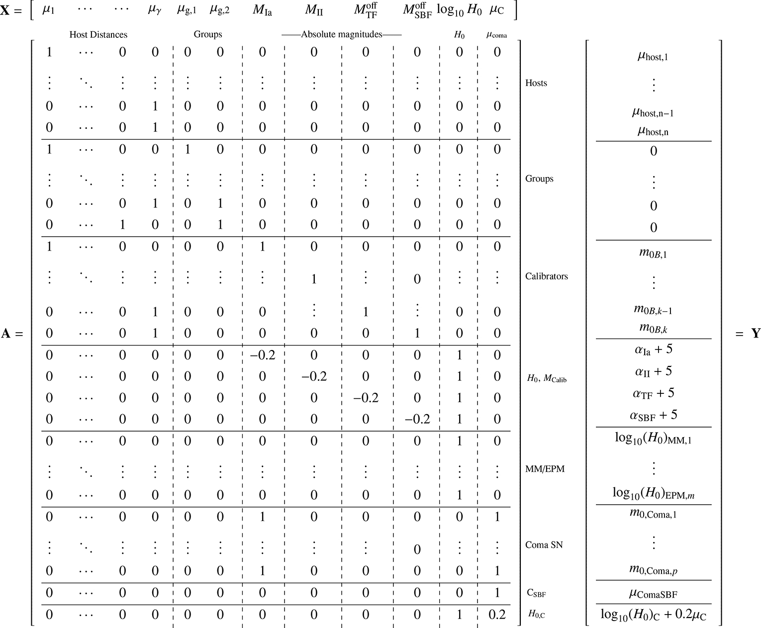
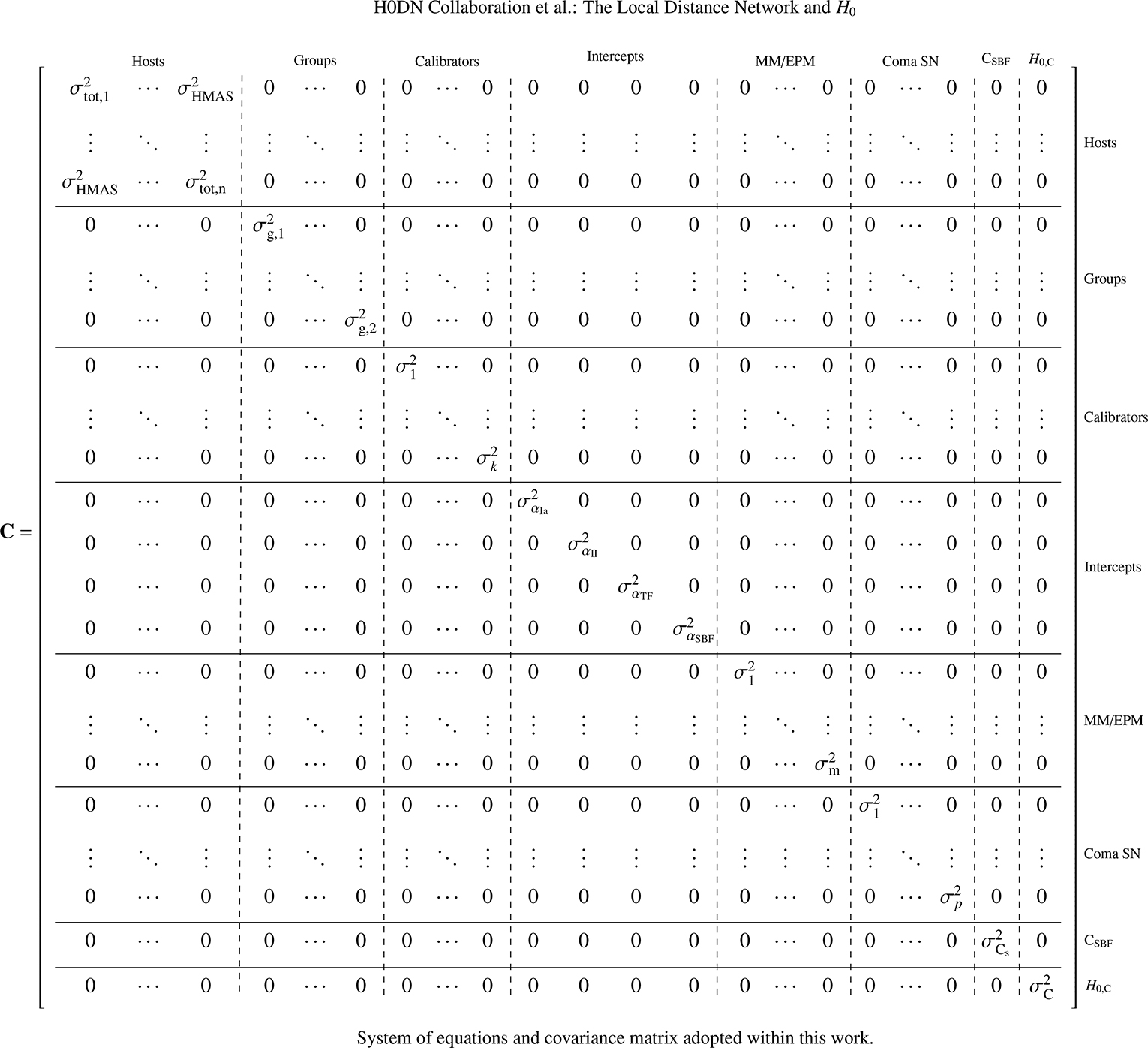
Appendix C: Literature comparison
Given that the distance network is an extension of the distance ladder framework, it is only natural, and an important test, that we should be able to reproduce various literature results using this framework. A few caveats to this arise from the simplifications we made in order to build the distance network, as well as possibly different treatments of objects in the Hubble flow (e.g., different peculiar velocity treatments). However, these are not expected to cause significant differences (≲0.3 km s−1Mpc−1) in the final determination of H0.
C.1. Literature replication and comparison for SNe Ia
Given the dominant role of the SNe Ia in previous claims of a Hubble tension, we focus in this part of the appendix on the agreement of the SNe Ia-derived results by exploring a broader range of SN Ia light curve fitters and SN Ia calibration samples than those included in the main variants Sect. 5 that may help explain the origin of differences in H0 compared to literature studies.
First, we compare our distance network in the case that we only use SNe Ia as secondary distance indicators and in the Hubble flow. For this case, we can compare to three references, namely Riess et al. (2022b), Dhawan et al. (2023), Freedman et al. (2025). This comparison is graphically summarized in Figs. C.1 and C.3, and the corresponding numbers can be found in Tables C.1 and C.4. We observe that all comparisons agree between the publication and the Distance Network emulation within less than 0.15σ on the inferred value of H0. In particular, when using only the 42 calibrators of Riess et al. (2022b) for Pantheon+ supernovae and adopting only the Cepheid calibration as in that study, we find H0 = 73.17 ± 0.96 km s−1 Mpc−1 where they find H0 = 73.15 ± 0.97 km s−1 Mpc−1 (0.02σ difference, 1% smaller uncertainty). Note that we compared to the results of Riess et al. (2022a), as the Distance Network also includes the cluster Cepheids that tighten the calibration in the anchors. When comparing to the Cepheid-based results of Dhawan et al. (2023) based on BayesSN supernovae, we find in this case H0 = 74.67 ± 1.14 km s−1 Mpc−1 where they find H0 = 74.82 ± 1.28 km s−1 Mpc−1 (−0.12σ difference, 11% smaller uncertainty). In this case, there is an additional caveat that Dhawan et al. (2023) only used 41 calibrators whereas with the BayesSN supernova fitter we used 42 Cepheid calibrators in this case. Finally, when comparing to the 24 TRGB-calibrated SN Ia results of F25, we find H0 = 70.31 ± 1.80 km s−1 Mpc−1 where they find H0 = 70.39 ± 1.22 (stat) ± 1.33 (sys) ± 0.70 (σSN) km s−1 Mpc−1 (−0.06σ difference, 0.3% smaller uncertainty when comparing the relevant uncertainties in quadrature). We can also compare the values of the calibration in these cases, finding for Riess et al. (2022b)MB = −19.260 ± 0.027 (−0.18σ compared to MB = −19.253 ± 0.027), for Dhawan et al. (2023)ΔMB = 0.039 ± 0.027 (+0.4σ compared to ΔMB = 0.030 ± 0.023, with one additional calibrator), and for Freedman et al. (2025)MB = −19.186 ± 0.053 (−0.11σ compared to MB = −19.18 ± 0.04(statonly)). We thus take as a noteworthy conclusion that the DN can accurately reproduce the individual distance ladder results based on the host distances, standardized SN magnitudes, and geometric calibrations used in these studies.
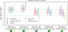 |
Fig. C.1. Comparison of the impact of supernova type Ia calibrator samples (sets of hosts) on the Hubble constant inference H0, each one relative to the baseline result, for the various light curve fitting codes. The triangle shows a case where for the bayesSN fitter only 52 out of the 55 hosts was calibrated due to several missing supernovae in the fit, and the cross one where only 32 out of 35 hosts were calibrated. (For details on the pie charts, see Fig. 13.) In this case we take 100% of the pies to be the case involving all supernovae data instead of the baseline. |
Comparison of Hubble constant values from different supernova sets and calibrators.
C.2. Understanding differences in H0 for past SN Ia-based ladders
Since we can reproduce the literature results within our framework, we can also investigate the sources of differences in H0 which may be attributed to specific analysis choices and datasets.
C.2.1 Refitting with new, SNooPy v2.7.0
An immediate challenge to comparing and extending the SN Ia results that make use of the SNooPy fitter (used in all CSP and CCHP studies) is both the absence of many useful SN calibrators in the Uddin et al. (2024, hereafter U24), the compilation that was used in Freedman et al. (2025) (hereafter F25), as well as the update of the SNooPy fitter to version v2.7.0 or later (since Aug 27, 2024); the prior version, which we dub “pre v2.7,” (the prior release was 2.5.3 Jan 29, 2020) that was used in U24 is not readily accessible nor recommended for further use by its author. According to C. Burns, who supports SNooPy development (private communication, 2025), current studies are advised to use the latest, v2.7.0. The most relevant update in v2.7 involves the method used by SNooPy to extrapolate the light curve templates beyond the training sample (s(B − V) < 0.3 and s(B − V) > 1.27). Supernovae that have light curves and inferred luminosities near the extrema of the distributions are often described as “91bg-like” at the faint and fast side and “91T-like” at the bright and slow, or high stretch, side. This has very little affect on the sample of calibrators, which are often preselected to be normal or near the middle of the distribution (see R22). However, the Hubble flow sample, and specifically the CSPII sample, has a surprising abundance of “high-stretch” or 91T-like SNe Ia (U24). We find 18 such supernovae in CSPII and 5 in CSP I (so 23 in all). Such SNe Ia will generally have s(B − V)≥1.15, for which the impact from the version update is quite large. The prior SNooPy version (pre v2.7) was found to over-correct these, motivating the revision to the fitter. For the updated SNooPy v2.7, prior fits with s(B − V)∼1.15 are lowered on average to s(B − V)∼1.0 (the fit, apparent peak magnitudes are hardly impacted) and the implied reddening in B − V is increased by ∼ 0.04 mag. The net change comparing old and new follows as Δm ≈ 0.9 ⋅ (1.15 − 1.0)−2.9 ⋅ ( − 0.04)≈0.25 mag (neglecting a small quadratic term in s(B − V) for this illustration) for the high s(B − V) supernovae, with the new standardized magnitude being brighter (since a brightness previously attributed to over-luminosity and low extinction is now reflected in the newly, brighter standardized magnitudes). Specific examples that all have s(B − V) > 1.1 include CSP12G, CSP13Z, CSP13aad, LSQ12agd, LSQ12gef, LSQ12hxx, LSQ13dqh, and PTF14uo, which all change by 0.2-0.3 mag in the same brighter direction. As 91Ts represent ∼ 8% of the CSP sample, we might expect a mean change of ∼ 0.02 mag, which is similar to the actual change from the new version of ∼0.03 mag (which includes error weighting). This appears as an increase in the Hubble flow intercept of aB = 0.6843 ± 0.0025 to aB = 0.6895 ± 0.0026 ( + 2σ). As a result H0 increases by 1.0 km s−1Mpc−1 due only to the change in the measurement of the Hubble flow for CSP from the new SNooPy.
An independent consideration is that it is also necessary to use the newer SNooPy v2.7 to fit additional SN Ia calibrators not included in the U24 compilation produced from pre v2.7 SNooPy. New SNooPy v2.7 fits were thus made by C. Burns (private communication, 2025) using the versions of the light curves in the Pantheon+ light curve database, most of which are not CSP light curves. In the process a number of discrepancies were identified from the prior SNooPy fits in U24 and Freedman et al. (2019, hereafter F19). These were either the use of an older data release when a newer and better one was available (e.g., Cfa I from Riess et al. 1999 did not employ host subtraction that was applied and released in Riess et al. 2005, 2007), an inconsistency in a filter function definition (i.e., when older published data were provided after transformation to the Landolt/Bessel system, not the “natural” system, e.g., 1998bu and 2002fk) or the use of a broader set of optical light curves was available.
These differences tend to pertain to older light curves from CfA I or LOSS, with changes in either direction, as tabulated in Table C.2.
Differences in SN Ia lightcurve data adopted in F19/U24/F25 compared to the best available data.
Due to the rarity of NIR light curves for calibrators that span decades and require data before NIR observations were common, to avoid introducing a systematic error (from the difference between optical and NIR calibration) we did not include NIR data for the CSP Hubble flow (in practice we found this difference is negligible). (See, however, 5.1 for variants that specifically use only NIR information for both calibrators and Hubble flow.)
The net change from SNooPy pre-v2.7 to post-v2.7 makes the mean calibrator fainter in MB by 0.026 mag for the F25 sample of 24 SNeIa and 0.019 mag for the full in-common sample of 35 SNeIa. Overall, compared to prior SNooPy fits, the fits of the current version (SNooPy v2.7) raise H0 for the same SN samples by ∼1.7 km s−1 Mpc−1 (e.g., from 70.31 for the F25 sample to 72.05). This difference is caused then primarily from improvements to SNooPy and to a lesser degree from better, later versions of the SN Ia calibrator data (see Table C.3).
Dependence of H0 on SNooPy fitter version and SN sample for TRGB ladder.
C.2.2 Differences with calibrator sample size
Lastly, within the use of every SN fitter, increasing the sample size from the smallest, selected study (the F25 sample of 24 calibrators) to the full available sample of 55 calibrators shows a clear trend toward increasing H0—as evident from Fig. C.1 and Table C.1. It increases by 0.9km s−1 Mpc−1 for Pantheon+ fitting, by 0.2km s−1 Mpc−1 for SNooPy post-v2.7 fitting, by 1.0km s−1 Mpc−1 for Salt 3 fitting, and by 1.4km s−1 Mpc−1 for BayesSN fitting—a mean of +0.9 km s−1 Mpc−1. This difference due to calibrator sample is even greater between the F25 sample and that from R22, about 1.2 km s−1 Mpc−1 in the mean, agreeing with the findings of Riess et al. (2024). This is shown in Fig. C.1. It seems reasonable to expect greater convergence in estimates of H0 as sample sizes increase.
We note that the F25 sample is not a natural sample selection from the perspective of the Distance Network—it cannot be constructed from simple cuts in redshift/distance or calibrator type. As such, we do not consider it as a variant (according to the methodology laid out in Sect. 2.4.2, those should be based on physical assumptions or hypotheses). We analyze it here to provide for a direct comparison with Freedman et al. (2025). We show the distribution in distance of the F25 (N = 24) and full samples (N = 55) according to the network in Fig. C.2, which shows that 37 of the 55 objects would have to be included if a cut was made in distance modulus to retain the full F25 sample. The smaller F25 sample is at a mean distance modulus of μhost = 31.13 ± 0.85, and the remaining sample is at a mean distance modulus of μhost = 32.01 ± 0.73, which are thus a little farther away on average (though not very significantly).
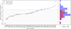 |
Fig. C.2. Full network sample (blue) and the F25 sample of calibrator hosts (red) in comparison. The gray region marks the maximal extent of the F25 sample. The green stars mark hosts with TRGB distances available. The left hand side shows an ordered scatterplot of the distance moduli, while the right hand side shows the corresponding histogram. Note that while F25 calibrates 24 SN Ia, these are located in only 20 hosts (hence only 20 points are marked red). The 11 additional hosts marked with green stars would correspond to potentially 10 additional SNe Ia (with the 11th host NGC 1399 calibrating SBF, not SNe Ia). One additional SN Ia (2021pit) is present in an already F25-calibrated host (N5643) but not within the CSP sample. In total that makes 24+10+1 = 35 calibrators that are available for SNe Ia calibrated through TRGB. Even within the sample of the CSP I&II supernovae only, there would still be 4 additional CSPI&II calibrators to be gained using TRGB observations of nearby hosts within the range of the F25 sample—with 7 additional TRGB-calibratable SNe Ia not present within the CSP I&II samples. The 4 “missing” TRGB-F25 calibrators are 2012ht in NGC 3447, 1998aq in NGC 3982, 1992A in NGC 1380, and ASAS14-lp in NGC 4666. |
For this purpose we can also look at Fig. C.3, which shows the differences between calibrator sets for the same supernovae standardizations and datasets. In each case we take the same supernovae to be used for calibration, but vary with which primary distance indicators the distances to their hosts are calibrated, for example using only HST Cepheids versus using all methods, or using only the TRGB (JWST and HST) vs using all methods, or using only the TRGB calibrations adopted in F25 versus using all methods. These differences are typically compatible with the uncertainty at ∼1σ, with shifts around −1km s−1 Mpc−1 in central value. We also observed that the reduced calibrations agree nicely with the results reported in the literature.
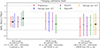 |
Fig. C.3. Comparison of H0 between different ways of calibrating a given set of hosts and a gievn SN fitter. It is computed as the result with the hosts calibrated through any means minus the result with the hosts calibrated through a specific calibration type (such as only Cepheids, only TRGB, or only F25 TRGB). The results with the star mark the literature results for the given (reduced) set of calibrating a given set of hosts. The triangle shows a case where for the BayesSN fitter only 32 out of the 35 hosts were calibrated due to several missing supernovae. |
C.3 Literature comparison for other distance indicators
Next, we compare our distance network to the case where we use other distance indicators. The results can be found in Fig. C.4 and Table C.4. These results are generally very consistent with the literature results, deviations typically staying at 0.1σ or less, once the same configuration is enforced.
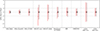 |
Fig. C.4. All literature comparisons for the given configuration/method (see x-axis label and main text). The light red results are the results for the given configuration/method coming from the Distance Network, while the dark red results are those available in the literature (differences are always zero but illustrates literature uncertainties; see also Table C.4). |
Comparison between recent literature results and DN emulation with the same data.
The SNII standard candle method naively appears to give discrepant results “out-of-the-box” in the distance network compared to the results from de Jaeger et al. (2022). However, this is due to the change in calibration described in Appendix A.3.2, where we only use 9 out of the 13 possible supernovae as described in that appendix. If we adopt the precise calibration of de Jaeger et al. (2022), we recover their value very closely. For the megamasers of Pesce et al. (2020b), we recover the value without any changes. However, it is important to compare with the correct value, as our baseline employs 2M++ velocity corrections, and does not include N4258 as a nonanchor megamaser. For surface brightness fluctuations (SBF), it is important to correct the literature value for the impact of peculiar velocities manually, which we do by using the difference from peculiar velocities from Blakeslee et al. (2021, which is ΔH0 = +0.27 km s−1 Mpc−1) and applying that to the value of Said et al. (2025), correcting the central value from 73.9 to 74.17 km s−1 Mpc−1. We assume no further changes in the uncertainty. For the astrophysical modeling of type II supernovae, using the tailored EPM (EPM), we can directly reproduce the literature value within great agreement. For the Coma-derived value we check both values derived using only the SBF calibration or using only the supernovae from Riess et al. (2022b). In both cases the result has excellent agreement with the literature value. Finally, we note that we did not manage to recover the literature value of the TF relation, but private communication with P. Boubel revealed that there might have been an issue in their code, leading to an incorrect value. This only affects Boubel et al. (2024b); future work will be based on the data in earlier publications, which were not available to us at the time of this analysis.
Appendix D: Sensitivity of the baseline to the distance to NGC 4258
Given the prominent role of NGC 4258 in the distance network, it may be of interest to consider the degree to which the baseline results depend on the accuracy of the distance to NGC 4258. Such a change is easily evaluated using the distance network by shifting distances with direct trace to NGC 4258 calibration. For the baseline, the distance to NGC 4258 of D = 7.58 ± 0.11 Mpc comes from Reid et al. (2019). In Table D.1 we show extreme cases of raising or lowering the distance by ±5% and ±10% (many times the stated uncertainty while retaining the uncertainty). These would lower/raise H0 by 1.3% and 2.6%, respectively, or approximately 25% of the change in the distance to NGC 4258. The relative size of the change in H0 compared to that of the anchor distance is mitigated by the availability of the other anchors from Gaia parallaxes and DEBs in the Magellanic Clouds (i.e., it would be a 33% change in H0 of the change in distance for NGC 4258 if these 3 anchors had equal weight). More importantly, such large shifts are strongly disfavored by the distance network goodness of fit as in either case the χ2 increases significantly, by 15 for the increased distance and by 38 for the decreased distance as shown in Fig. D.1. This is consistent with the finding of variant V12, which removes NGC 4258 from the baseline resulting in H0 = 73.1 ± 0.92 km s−1 Mpc−1, representing only a small decrease of 0.4 km s−1 Mpc−1 and an increase in the error by only 15%. This shows that the literature N4258 distance is compatible with the remainder of the Distance Network and strong deviations are incompatible, and the presence of the N4258 anchor is not crucial for the Distance Network.
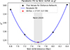 |
Fig. D.1. Trial values for the distance to NGC 4258 and associated χ2 values. Besides the Reid et al. (2019) measure at D = 7.58 ± 0.11 Mpc (shown as gray band) we also tried increasing or decreasing the distance by ±5% and 10% (black crosses). The result its a large internal inconsistency in the distance network (due to other geometric anchors) that is highly significant. (See also Table D.1 for impact to H0). The global minimum (vertex) is marked by a red cross. |
Sensitivity of baseline to large changes in NGC 4258 distance.
We conclude that the Hubble tension is relatively insensitive to the stated accuracy of NGC 4258 alone.
Appendix E: Additional details from the Distance Network: Calibration parameters and host/calibrator distances
The main result of the Distance Network analysis is of course the value and uncertainty of H0, reported in Table 4 for all variants, together with the value of the total χ2 to evaluate the quality of the fit. In addition, the Distance Network process can provide more detailed information on each class of calibrators and on host and the calibrated distances.
E.1. Calibration parameters
The Distance Network approach can include several secondary distance indicators whose calibration is determined simultaneously with all other parameters of the solution; each can be used to constrain H0 via tracers in the Hubble flow. For each variant, Table E.1 provides the resulting calibration parameter, the Hubble flow intercept, and the number of calibrators for each of the main secondary distance indicators: SNe Ia, SBF, SNe II, and TF. For SNe Ia and SN II, the calibration parameter is generally the reference absolute magnitude of a standardized SN in the appropriate passband; the exception is the BayesSN method, which uses a different definition. For SBF and TF, the calibration parameter is reported as the difference with respect to the published value, as described in Appendix A. In all cases, the reported uncertainty is marginalized over all other parameters in the Distance Network.
Additional fit parameters for all variants.
The Hubble flow intercept is the parameter a𝒯 defined in Eq. B.15 and discussed in Section B.3.5. It is expressed in units of log(H0) (numerically equivalent to 0.2 mag); the reported uncertainty includes the intrinsic and measurement error for the tracers, but does not include the calibration uncertainty. For some versions of SNe Ia, the reported uncertainty includes covariance terms between different tracers, as reported in the original sources.
E.2. Host and calibrator distances
One of the secondary results of the Distance Network approach is an optimized set of distance moduli for all hosts and calibrators included in the Network. These distances are based not only on the multiple measurements included in the Distance Network, but also on the consistency equations for the various classes of calibrators to which they belong. They represent the values of the distances that, together, produce the best-fitting solution to all of the Distance Network equations. As a result, the estimated distances for each host will differ slightly depending on which classes of calibrators are included in the solution, even when no additional measurements are introduced.
Table E.2 reports the best distance estimate for each of the hosts (or host/calibrators) included in two solutions, Baseline (V00) and “everything,” the solution including all methods (V99). Since hosts not tied to any calibrators are excluded from each solution, many of the hosts do not have a distance estimate in the Baseline version. SN calibrators are not included, since their distances are not separate parameters; they are assumed identical to the distances to their host, which as a consequence are also affected by the SN calibration via the (one or more) SNe they host. On the other hand, SBF calibrator galaxies in Fornax and Virgo are included individually; their distances are allowed to deviate from the group distance, because of depth effects, and are affected by their SBF luminosity measurements via their global calibration. The quoted distance uncertainties are marginalized over all parameters of the respective Distance Network solution and are therefore not independent.
Distance moduli and statistical uncertainties for host and calibrator systems in the Distance Network.
All Tables
Comparison of Hubble constant values from different supernova sets and calibrators.
Differences in SN Ia lightcurve data adopted in F19/U24/F25 compared to the best available data.
Comparison between recent literature results and DN emulation with the same data.
Distance moduli and statistical uncertainties for host and calibrator systems in the Distance Network.
All Figures
|
Fig. 1. Conceptual overview of the Local Distance Network, a many-routes approach. Different methods for distance determination may connect the absolute scale determined by geometric means to H0. A nonexhaustive list of baseline linkages discussed in the literature or the paper is labeled on the right. Links to geometric distances provided by masers, DEB, and parallaxes are indicated as available in our analysis. Background rectangles in orange, light blue, and gray indicate where Rung 1, Rung 2, and Rung 3 of a traditional distance ladder would fall. Unlabeled tick marks represent groups (Fornax & Virgo for the TRGB to SBF, Coma for FP). Example references: Riess et al. (2022b, SH0ES), Freedman et al. (2025, CCHP), Anand et al. (2021, EDD), Anand et al. (2024b, Pop-II), Pesce et al. (2020a, MCP), de Jaeger et al. (2022, Pop-I), Kourkchi et al. (2020, CF4), Said et al. (2025, DESI), Vogl et al. (2025, adh0cc). Appendix C.1 replicates a subset of these routes. |
| In the text | |
|
Fig. 2. Complete Distance Network, with all possible pathways illustrated. Anchors are objects that establish an absolute scale based on the methods shown to their left. The primary distance indicators (Cepheids, TRGB, Miras, and JAGB) transfer the absolute scale to hosts (i.e., galaxies), the ensemble of which calibrates secondary distance indicators in the Hubble flow (tracers). Exceptions are Megamasers and astrophysically modeled SNe II, both of which serve as primary distance indicators and are capable of reaching the Hubble flow without intermediate steps. Green arrows illustrate direct connections between anchors or tracers and the method used to determine the absolute scale. Blue, violet, yellow, and red arrows show which calibrators constrain host distances; line width qualitatively distinguishes the attainable precision. Among hosts, rectangles qualitatively indicate overlap among objects measured via multiple methods. Diamond shapes represent groups. Dark gray arrows tie subsets of hosts whose distance is constrained by different calibrators to tracers. Any given arrow may represent multiple datasets, for example, HST or JWST photometry of Cepheids or optical versus infrared photometry of SNe Ia. The number of hosts is labeled for Cepheids, TRGB, JAGB, and Miras, with the number of hosts exclusively available to each method shown in parentheses. |
| In the text | |
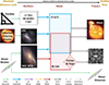 |
Fig. 3. Baseline Distance Network illustrated analogously to Fig. 2. |
| In the text | |
|
Fig. 4. Residuals for each category of host distance measurements from the Baseline solution. Each panel represents a group of measurements of host distances that share the same method, anchor, and authors, and shows the deviation of those measured host distances from the full Distance Network value. Error bars represent the individual uncertainty of each measurement, while the shaded regions for each group shows the common (fully correlated) uncertainty due to the reference system. |
| In the text | |
|
Fig. 5. Residuals in distance modulus as a function of redshift for objects in the Hubble flow in the Baseline solution. Error bars reflect the individual source scatter, without the common calibration uncertainty. The shaded region in each plot indicates the effect of a velocity uncertainty of 250 km s−1. The bars at the right show the mean and dispersion for each group of sources and the calibration uncertainty, which is a common error mode for all points in each panel. |
| In the text | |
|
Fig. 6. Corner plot for the baseline solution illustrating the correlations between H0, the calibration of SNe Ia and SBF, and the distance to Fornax and Virgo, which contribute to the SBF calibration. The parameters use the naming convention of Appendix B.3.1. Deviations from the analytically calculated result are due to the numerical precision of a finite-length chain. |
| In the text | |
|
Fig. 7. Comparison of the baseline result with previous literature results based on early Universe indirect inferences using the flat ΛCDM model, based on direct measurements in the late Universe, and based on strong lensing results (which involve additional modeling). |
| In the text | |
|
Fig. 8. Baseline and variants results from Table 4. For some variants, a labeled change has a secondary consequence (i.e., removing the identified primary distance indicator also results in the loss of calibration to some SN Ia). In these cases a dashed line immediately below such variants provides a custom baseline–i.e., the same SNe are removed before the removal of the primary indicator–is shown to provide a custom reference of the impact for that variant (see text for details). |
| In the text | |
|
Fig. 9. Residuals for host and calibrator distances for the “everything” solution. The groupings, also distinguished by color, correspond to calibrators measured by the same authors with a common method and anchor. The error bars reflect the individual calibrator errors. The shaded areas for each group indicate the combined uncertainty in the anchor distance and its reference value, which are in common for all calibrators in the same grouping. |
| In the text | |
|
Fig. 10. Residuals in log(H0) versus redshift for objects in the Hubble flow for the “everything” solution. Each subplot refers to sources in the same group, measured by the same method. Error bars for individual sources are representative of the expected scatter across sources in the same category and do not include calibration uncertainties for each class. The shaded bars at the right show the mean and dispersion for each category. |
| In the text | |
|
Fig. 11. Corner plot illustrating the main optimization parameters for the all-inclusive solution. The naming convention of Appendix B.3.1 is used. Parameters related to individual host distances are not included. Note that this solution is not an alternative result to the baseline solution, but rather it is a variant to check the impact of further data on our result (see also Sect. 5). We show it here to highlight the existing correlations between the various (most important) solution parameters. Deviations from the analytically calculated result are due to the numerical precision of a finite-length chain. |
| In the text | |
|
Fig. 12. Illustration of H0 estimates resulting from orthogonal paths. The two paths starting with “O” are proper orthogonal paths and can be taken as independent measurements of the Hubble constant. Their weighted mean (red) agrees well with our baseline result despite the latter including all cross-correlations. The shortcuts of the datasets are as defined in the text. The pie charts “fraction of data kept” represent the fraction of statistical power remaining in the path. It is computed as the fraction of the variance of H0 for the given result (in this way multiple datasets with the same constraining power in H0 will be assigned equal percentages). We show the percentages relative to the baseline result (V00). |
| In the text | |
|
Fig. 13. Statistical consistency of various individual paths through the network. These estimates represent a set of paths that are highly correlated, and they often only take a tiny part of the network into account. They are used for a statistical consistency check and should not be interpreted as valid variants in the sense of Sect. 2.4.2. We also show the simple weighted mean of these paths in gray purely for visual purposes, reminding that due to their correlations (and selection effects) it need not necessarily agree with the baseline result. For details on the pie charts, see Fig. 12. |
| In the text | |
|
Fig. C.1. Comparison of the impact of supernova type Ia calibrator samples (sets of hosts) on the Hubble constant inference H0, each one relative to the baseline result, for the various light curve fitting codes. The triangle shows a case where for the bayesSN fitter only 52 out of the 55 hosts was calibrated due to several missing supernovae in the fit, and the cross one where only 32 out of 35 hosts were calibrated. (For details on the pie charts, see Fig. 13.) In this case we take 100% of the pies to be the case involving all supernovae data instead of the baseline. |
| In the text | |
|
Fig. C.2. Full network sample (blue) and the F25 sample of calibrator hosts (red) in comparison. The gray region marks the maximal extent of the F25 sample. The green stars mark hosts with TRGB distances available. The left hand side shows an ordered scatterplot of the distance moduli, while the right hand side shows the corresponding histogram. Note that while F25 calibrates 24 SN Ia, these are located in only 20 hosts (hence only 20 points are marked red). The 11 additional hosts marked with green stars would correspond to potentially 10 additional SNe Ia (with the 11th host NGC 1399 calibrating SBF, not SNe Ia). One additional SN Ia (2021pit) is present in an already F25-calibrated host (N5643) but not within the CSP sample. In total that makes 24+10+1 = 35 calibrators that are available for SNe Ia calibrated through TRGB. Even within the sample of the CSP I&II supernovae only, there would still be 4 additional CSPI&II calibrators to be gained using TRGB observations of nearby hosts within the range of the F25 sample—with 7 additional TRGB-calibratable SNe Ia not present within the CSP I&II samples. The 4 “missing” TRGB-F25 calibrators are 2012ht in NGC 3447, 1998aq in NGC 3982, 1992A in NGC 1380, and ASAS14-lp in NGC 4666. |
| In the text | |
|
Fig. C.3. Comparison of H0 between different ways of calibrating a given set of hosts and a gievn SN fitter. It is computed as the result with the hosts calibrated through any means minus the result with the hosts calibrated through a specific calibration type (such as only Cepheids, only TRGB, or only F25 TRGB). The results with the star mark the literature results for the given (reduced) set of calibrating a given set of hosts. The triangle shows a case where for the BayesSN fitter only 32 out of the 35 hosts were calibrated due to several missing supernovae. |
| In the text | |
|
Fig. C.4. All literature comparisons for the given configuration/method (see x-axis label and main text). The light red results are the results for the given configuration/method coming from the Distance Network, while the dark red results are those available in the literature (differences are always zero but illustrates literature uncertainties; see also Table C.4). |
| In the text | |
|
Fig. D.1. Trial values for the distance to NGC 4258 and associated χ2 values. Besides the Reid et al. (2019) measure at D = 7.58 ± 0.11 Mpc (shown as gray band) we also tried increasing or decreasing the distance by ±5% and 10% (black crosses). The result its a large internal inconsistency in the distance network (due to other geometric anchors) that is highly significant. (See also Table D.1 for impact to H0). The global minimum (vertex) is marked by a red cross. |
| In the text | |
Current usage metrics show cumulative count of Article Views (full-text article views including HTML views, PDF and ePub downloads, according to the available data) and Abstracts Views on Vision4Press platform.
Data correspond to usage on the plateform after 2015. The current usage metrics is available 48-96 hours after online publication and is updated daily on week days.
Initial download of the metrics may take a while.