| Issue |
A&A
Volume 708, April 2026
|
|
|---|---|---|
| Article Number | A112 | |
| Number of page(s) | 29 | |
| Section | Extragalactic astronomy | |
| DOI | https://doi.org/10.1051/0004-6361/202557396 | |
| Published online | 01 April 2026 | |
MUSE-DARK
I. Dark matter halo properties of intermediate-z star-forming galaxies
1
Univ. Lyon1, Ens de Lyon, CNRS, Centre de Recherche Astrophysique de Lyon (CRAL), 69230 Saint-Genis-Laval, France
2
Aix Marseille Univ, CNRS, CNES, LAM, Marseille, France
3
Leibniz-Institut für Astrophysik Potsdam (AIP), An der Sternwarte 16, 14482 Potsdam, Germany
4
Institut de Recherche en Astrophysique et Planétologie (IRAP), Université de Toulouse, CNRS, UPS, CNES, 31400 Toulouse, France
★ Corresponding author: This email address is being protected from spambots. You need JavaScript enabled to view it.
Received:
24
September
2025
Accepted:
12
February
2026
Abstract
Context. The core–cusp problem is a key challenge to the Lambda cold dark matter (ΛCDM) model. Stellar feedback and other baryonic processes have been proposed as solutions to reconcile the tension between the predicted cuspy profiles and the observed cores of low- and intermediate-mass galaxies. However, at z > 1, disk–halo decompositions usually focus on massive star-forming galaxies (SFGs) with log(M★/M⊙) > 10, as observations typically lack the depth and sensitivity to probe lower-mass systems, where cores are predicted to occur.
Aims. For this study we analysed the dark matter (DM) halo properties of 127 intermediate-redshift (0.3 < z < 1.5) SFGs down to low stellar masses (8 < log(M★/M⊙) < 11), using the highest signal-to-noise data from the MUSE Hubble Ultra Deep Field Survey, as well as photometry from the Hubble Space Telescope and James Webb Space Telescope.
Methods. We employed a traditional 2D line fitting algorithm and a 3D forward modelling approach to analyse the kinematics of our sample, enabling us to measure individual rotation curves extending up to two to three times the effective radii. We performed a disk–halo decomposition with a 3D parametric model, which includes stellar, DM, and gas components, as well as corrections for pressure support. We tested our methodology using mock data cubes generated from idealised disk simulations, and we performed several cross-checks, such as comparing our 3D disk–halo decomposition with results obtained from external data, as well as 1D decompositions, finding good agreement. We tested six DM density profiles, including the Navarro–Frenk–White, Burkert, Einasto and the generalised αβγ profile of (Di Cintio, A., Brook, C. B., Dutton, A. A., et al. 2014, MNRAS, 441, 2986, DC14), as well as a baryon-only model using a Bayesian analysis.
Results. Marginalising against the unknown neutral gas content, we find that the mass-dependent DC14 DM profile, which accounts for the response of DM to baryonic processes such as stellar feedback, performs as well as or better than the other halo models for most of the sample (≳80%), and that baryon-only models seem to be disfavoured with respect to DM models for 84% (107/127) of the galaxies. We find that 89% of the SFGs have DM fractions (fDM(< Re)) larger than 50%, and we extend the fDM(< Re)−ΣM★ relation at lower masses. Using DC14 DM profiles, we infer DM inner slopes γ < 0.5 for 66% of the sample, indicative of cored DM density profiles. The stellar–halo mass and concentration–halo mass relations inferred from our 3D modelling agree with the theoretical expectations, albeit with larger scatter. Our results confirm the anti-correlation between the halo scale radius and DM density with a slope of ∼ − 1, which seems to evolve with redshift. While the halo scale radii are z-invariant, we find tentative evidence that DM halos of z ∼ 1 SFGs were denser (by ∼0.3 dex) than those in the local Universe.
Conclusions. We measured DM halo properties of intermediate-z SFGs down to 108 M⊙, and find that a substantial fraction of the sample can be described by cored DM density profiles. This may point towards core formation driven by baryonic processes in the context of ΛCDM.
Key words: galaxies: evolution / galaxies: halos / galaxies: high-redshift / galaxies: kinematics and dynamics
© The Authors 2026
 Open Access article, published by EDP Sciences, under the terms of the Creative Commons Attribution License (https://creativecommons.org/licenses/by/4.0), which permits unrestricted use, distribution, and reproduction in any medium, provided the original work is properly cited.
This article is published in open access under the Subscribe to Open model. This email address is being protected from spambots. You need JavaScript enabled to view it. to support open access publication.
1. Introduction
The matter content of the Universe is dominated by dark matter (DM) from subgalactic to cosmological scales. The concept of DM entered mainstream research in the 1970s when observations revealed that galaxy rotation curves (RCs) remain flat at large galactocentric distances (e.g. van de Hulst et al. 1957, Rubin & Ford 1970), contrary to the expected Keplerian decline. These flat RCs could not be explained by the Newtonian gravity of the baryonic matter alone, but instead suggested the presence of an extended DM halo.
Dark matter halos are a cornerstone of the Lambda cold dark matter (ΛCDM) cosmological model, which is a successful framework for predicting and explaining the large-scale structures of the Universe and their evolution with cosmic time. However, on scales smaller than ∼1 Mpc, this model faces several challenges (see Bullock & Boylan-Kolchin 2017 for a review). For example, DM-only simulations predict that DM assembles into halos that develop steeply rising inner radial density profiles, i.e. cusps, in the absence of any baryonic effects. These simulated DM halos can be described by ρ(r) ∝ r−γ with γ ∼ 0.8 − 1.4, and are well fitted by a Navarro–Frenk–White profile (NFW; Navarro et al. 1997, Klypin et al. 2001), independently of initial conditions and cosmological parameters. On the other hand, observations of low surface brightness galaxies have demonstrated that these systems show density profiles that are consistent with a constant-density core at the centre, with γ ∼ 0 − 0.5 (e.g. Flores & Primack 1994, Salucci & Burkert 2000, de Blok et al. 2001, Weldrake et al. 2003, Salucci et al. 2007, Oh et al. 2015). This disagreement between observations and simulations is known as the core–cusp problem and has posed a major challenge to ΛCDM for the past two decades (de Blok 2010). This discrepancy either hints at the inadequacy of DM-only simulations to capture the DM dynamics on small scales, due to the absence of phenomena connected to baryonic physics, or suggests that a modification of the whole ΛCDM paradigm is needed (e.g. self-interacting DM – Spergel & Steinhardt 2000, axion-like fuzzy DM- Hu et al. 2000).
Several baryonic mechanisms within the ΛCDM framework have been proposed to solve the core–cusp problem. For example, infalling gas clumps can transfer angular momentum to DM via dynamical friction, resulting in a shallower central density profile (e.g. El-Zant et al. 2001, Romano-Díaz et al. 2008, Johansson et al. 2009). Alternatively, energy could be transferred to the outer halo through resonant effects induced by a central stellar bar, which can also transform cusps into cores (Weinberg & Katz 2002). Cores may also be created when baryons, after condensing at the centre of a halo, are suddenly expelled by feedback processes. In many high-resolution cosmological simulations, strong stellar feedback from massive stars and supernovae was shown to drive large-scale gas outflows during repeated starburst events, leading to an overall expansion of the DM halo and the creation of a cored DM density profile (Navarro et al. 1996, Read & Gilmore 2005, Governato et al. 2010, Pontzen & Governato 2012, Teyssier et al. 2013, Brooks & Zolotov 2014, Freundlich et al. 2020a, Dekel et al. 2021, Li et al. 2023, Jackson et al. 2024, Azartash-Namin et al. 2024). Core formation can also be linked to active galactic nucleus (AGN) activity in high-mass galaxies and galaxy clusters (Martizzi et al. 2012, Peirani et al. 2017).
In the stellar feedback scenario, many studies claim that core formation is strongly dependent on M★/Mhalo, and that this mechanism is most efficient for (M★/Mhalo)∼3 − 5 × 10⁻³, corresponding to a stellar mass regime of 109 < M★/M⊙ < 1010. In more massive halos, the outflows become ineffective at flattening the inner DM density, and the halos have increasingly cuspy profiles. Similarly, at M★/Mhalo < 10−4, there is not enough supernova energy to efficiently change the DM distribution, and the halo retains the original NFW profile (Di Cintio et al. 2014, hereafter DC14; Read et al. 2016, Lazar et al. 2020, Azartash-Namin et al. 2024). Similar results were obtained from simulations that also include AGN feedback in addition to stellar feedback (e.g. Macció et al. 2020). Tollet et al. (2016) have demonstrated that the relationship between the inner DM density slope and M★/Mhalo holds approximately up to z ∼ 2, implying that in all halos, the shape of the inner density profile changes over cosmic time as they grow in stellar and total mass. Nevertheless, the dependence of the DM inner slope on M★/Mhalo is not universally seen across all hydrodynamical simulations (e.g. Bose et al. 2019).
Rotation curves are fundamental tools for probing the mass distribution in star-forming galaxies (SFGs) as they provide one of the few direct observables of the DM density on galactic scales (Rubin et al. 1978). In the local Universe, kinematic studies have employed various dynamical tracers to characterise the DM halo properties of disk galaxies (Kormendy & Freeman 2016, Katz et al. 2017, Allaert et al. 2017, Katz et al. 2018, Read et al. 2019, Korsaga et al. 2019, Salucci 2019, Li et al. 2019, Li et al. 2020, Mancera Piña et al. 2025). Beyond mapping the structure of local DM halos, understanding their evolution over cosmic time is crucial, thus making kinematic studies of higher-z galaxies essential for constraining the nature of DM.
Fortunately, over the past decade, deep Integral Field Unit (IFU) observations (e.g. Förster Schreiber et al. 2009, Genzel et al. 2011, Wuyts et al. 2016, Bacon et al. 2017, Wisnioski et al. 2015, Girard et al. 2018, Le Févre et al. 2020) using instruments such as the Spectrograph for INtegral Field Observations in the Near Infrared (SINFONI; Eisenhauer et al. 2003), the Multi-Unit Spectroscopic Explorer (MUSE; Bacon et al. 2010), the K-band Multi-Object Spectrograph (KMOS; Sharples 2014), the Near-Infrared Spectrograph (NIRSpec; Jakobsen et al. 2022), and submillimetre observations from facilities such as the Atacama Large Millimeter Array (ALMA), together with advancements in 3D modelling tools (Bouché et al. 2015, Di Teodoro & Fraternali 2015, Lee et al. 2025b), have opened a new avenue for probing the dynamics of high-z galaxies. Studying the DM halo properties of distant SFGs at z ≳ 1 requires very deep observations (Genzel et al. 2017, Genzel et al. 2020, Price et al. 2021, Puglisi et al. 2023, Nestor Shachar et al. 2023) or stacking techniques (Lang et al. 2017, Sharma et al. 2021, Tiley et al. 2019, Danhaive et al. 2026). Many of these studies often find declining outer RCs and consequently low DM fractions, but it is important to note that they primarily focus on high-mass systems (log(M★/M⊙)≳10). More recently, ALMA and the James Webb Space Telescope (JWST) have opened the possibility to study the properties of DM halos at z = 4 − 5 (Rizzo et al. 2021, Herrera-Camus et al. 2022, Roman-Oliveira et al. 2024, Lee et al. 2025a).
Some of these studies performed disk–halo decompositions (e.g. Genzel et al. 2020, Price et al. 2021, Fraternali et al. 2021, Nestor Shachar et al. 2023, Lelli et al. 2023, Roman-Oliveira et al. 2024, Nestor Shachar et al. 2025). In a pilot study of nine z ∼ 1 SFGs, Bouché et al. (2022) pushed this type of analysis on disk–halo decompositions to lower stellar masses (8.5 < log(M★/M⊙) < 10.5) using extremely deep MUSE observations (Bacon et al. 2017). They found a variety of RC shapes, reminiscent of the diversity observed at z = 0, DM fractions reaching > 60 − 95% in the lower-mass regime; 50% of the sample showed strong evidence of cored DM profiles.
In this paper (MUSE-DARK-I), we apply the same disk-halo decomposition technique used in Bouché et al. (2022) on a substantially larger sample of 127 SFGs at z ∼ 1. While Bouché et al. (2022) tested two DM density profiles (DC14 and NFW), here, with a larger sample of > 100 SFGs, we tested additional DM halo models, alongside a baryon-only model. Our galaxies span a wide range in redshifts (0.28 < z < 1.49) and stellar masses (7 < log(M★/M⊙) < 11), thus enabling us to explore how halo properties vary with both cosmic time and galaxy mass. To our knowledge, this represents one of the largest samples of distant SFGs with disk–halo decompositions analysed to date. Current studies are limited to small samples with 22 SFGs in Puglisi et al. (2023), 41 SFGs in Genzel et al. (2020), Price et al. (2021), and 100 SFGs in Nestor Shachar et al. (2023), most with log(M★/M⊙)≳10. With the series of MUSE-DARK projects, we aim to fill this knowledge gap by performing a detailed disk-halo decomposition analysis on a statistical sample of several hundred intermediate-redshift (0.2 < z < 1.5) SFGs with 8 < log(M★/M⊙) < 11 from the MUSE Hubble Ultra Deep Field (MHUDF, Bacon et al. 2023), the MUSCATEL (programme 1104.A-0026; PI: Wisotzki, L.) and the lensing cluster (Richard et al. 2021) datasets.
This paper is the first in a series focused on the MHUDF sample and is organised as follows. In Sect. 2 we present the methodology used to determine the morpho-kinematics of the sample, and we describe the 3D disk-halo decomposition. In Sect. 3 we validate our 3D methodology using mock data cubes generated from idealised disk simulations. Section 4 describes the observations employed in this study, as well as the data selection and global properties of the sample. The main results are presented in Sect. 5. In Sect. 6 we discuss the core formation scenario, as well as the caveats of this work. In Sect. 7 we present a summary and our conclusions.
Throughout this paper, we use a Planck 2015 cosmology (Planck Collaboration XIII 2016) with ΩM = 0.307, Λ = 0.693, and H0 = 67.7 km s−1 Mpc−1. With these cosmological parameters, 1″ subtends ∼8.23 kpc at z = 1. We also consistently use log for the base-10 logarithm. We assume a Chabrier (2003) initial mass function (IMF) for all the derived stellar masses and star formation rates (SFRs).
2. Methodology
To accurately probe the DM distribution in intermediate- to high-z galaxies, it is essential to measure RCs at large radii, up to 10 − 15 kpc, corresponding to 2 − 3 times the effective radii. However, at these large galactocentric distances, the S/N per spaxel of the emission line of interest drops below unity, making velocity measurements difficult without very deep observations (Genzel et al. 2017, 2020; Bouché et al. 2022; Nestor Shachar et al. 2023) or the use of stacking techniques (e.g. Lang et al. 2017; Tiley et al. 2019). Additionally, galaxies at z ≥ 0.5 are observed with spatial resolution (0.5″ or 4 kpc in diameter) comparable to their sizes, which span 3 − 5 kpc typically (e.g. Ward et al. 2024), meaning that these galaxies are only marginally resolved.
Fortunately, kinematic analyses of the DM distributions in distant SFGs are now feasible thanks to advancements in 3D forward modelling tools, such as GALPAK3D (Bouché et al. 2015), DYSMALpy (Übler et al. 2018, Price et al. 2021), and 3DBarolo (Di Teodoro & Fraternali 2015). These tools construct 3D disk models that can be directly compared to 3D observational data and are designed to disentangle galaxy kinematics from resolution effects by taking into account any instrumental effects (spatial or spectral resolution)1.
For this study, we used GALPAK3D, a full 3D forward modelling approach that fits the entire 3D cube directly rather than the measured 1D or 2D kinematics. This method is well suited for high-z systems where the spatial resolution and S/N are limited, beacuse (1) it uses all the spatial and spectral information contained in thousands of spaxels; (2) it allows the low S/N regions to be probed in the outskirts of galaxies, where the S/N of the spectral line of interest drops below unity, by leveraging the collective signal of all low S/N spaxels2; (3) it constrains the intrinsic morphological and kinematical parameters of the disk simultaneously, thereby breaking the vmax-inclination degeneracy; and lastly (4) it computes the likelihood directly from the 3D data without losing information. This framework assumes an axisymmetric disk, hence our rather strict criteria for selecting a sample of regular, unperturbed, rotation-dominated galaxies (see Sect. 4.2). We note, however, that non-axisymmetric features or non-circular motions could bias individual parameter estimates. For more details, we refer to Bouché et al. (2015) and Bouché et al. (2022).
First, we analysed the morpho-kinematics in order to select a sample of rotation-dominated SFGs with vmax/σ > 1 (see Sect. 4.2) using the 3D morpho-kinematic modelling (Sect. 2.1). Second, we performed a disk-halo decomposition (Sect. 2.2) using the methodology presented in Bouché et al. (2022).
In both cases, for the PSF and LSF in GALPAK3D, we used a circular Moffat PSF, as characterised by Bacon et al. (2023), and Eqs. (7) and (8) of Bacon et al. (2017) for the LSF. It is worth mentioning that in the wavelength range relevant for our emission lines, the MUSE velocity resolution is around ∼45–55 km s−1.
GALPAK3D optimises the model parameters (see Sect. 2.3) using various Markov chain Monte Carlo (MCMC) algorithms, and for this study, we used the Python version of MultiNest (Feroz et al. 2009, Buchner et al. 2014). The following pyMultiNest configuration was used for the bulk fits: 400 live points, sampling efficiency 0.8 and evidence tolerance 0.5, which is optimised for efficient and robust posterior estimation.
2.1. 3D morpho-kimematics approach
As described in Bouché et al. (2015, 2021), GALPAK3D builds a 3D model of a disk with a Sersic (1968) surface brightness profile, Σ(r), Sérsic index, ngas, and effective radius, Re. The disk model can be inclined to any inclination, i, and position angle (PA), whereas the thickness of the disk is assumed to be Gaussian, with a scale height hz = 0.15 × Re. For the disk kinematics, the model uses a parametric form for the RC, vc(r), and for the dispersion profile, σ(r).
The velocity profile vc(r) can be any functional form, and more details can be found in Bouché et al. (2015, 2021). Here, as in Bouché et al. (2022), we parametrised vc(r) using the universal RC (URC) from Persic et al. (1996), which allows both rising and declining RCs.
As described in Bouché et al. (2015, 2021), the velocity dispersion profile σ(r) consists of the combination of a thick disk σthick, defined as σthick(r)/vc(r) = hz/r, where hz is the scale height, and a dispersion floor, σ0, added in quadrature following Genzel et al. (2006), Cresci et al. (2009), Förster Schreiber et al. (2018), Wisnioski et al. (2015), Übler et al. (2019).
This 3D model has 13 parameters, including the [OII] doublet ratio (listed in Table A.1). As discussed in Bouché et al. (2022), there is generally a good agreement between the morphological parameters (Sérsic n, size, i) obtained from [OII] MUSE data with those obtained from HST. Here, we used priors on the inclination (see Sect. 2.3 for more information), while the other structural parameters were left free. While we do not show the comparison here, we verified that the structural parameters derived from MUSE are consistent with those obtained from HST/F160W (and stellar mass maps -see Sect. 4.3 for details on the photometric data), with a scatter of ∼0.14 dex in log(Re/kpc) and typical differences in Sérsic index of Δn ≲ 0.5 − 0.6.
2.2. 3D disk-halo decomposition
Following Bouché et al. (2022), we adopt a 3D disk-halo decomposition from the decomposition of the gravitational acceleration v2/r into the contributions from a DM component, vDM(r), a disk (stellar+molecular gas) component, vdisk(r), a neutral gas component, vH I(r), and when the bulge-to-total ratio, B/T > 0.2, an additional bulge component, vbulge(r), such that
 (1)
(1)
Compared to other high-z studies performing an RC decomposition (e.g. Genzel et al. 2017, Genzel et al. 2020, Nestor Shachar et al. 2023), we included an unknown H I neutral gas component, which we marginalised over. Also, compared to Bouché et al. (2022), we used vH I(r)|vH I(r)| to account for the possibility of a net outward force in the case of central HI mass depression (Casertano 1983). We did not apply the same treatment to the other components, as we do not expect them to exhibit central depressions that could result in a net outward force.
As in Bouché et al. (2022), Weijmans et al. (2008), Burkert et al. (2010), and others, we included a correction for pressure support P (sometimes called asymmetric drift), such that: vc2(r) = v⊥2(r)+vAD2(r), where 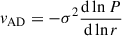 , with P being the pressure and σ the gas velocity dispersion in the radial direction. Following Dalcanton & Stilp (2010), we used the correction for turbulent star-forming disks, vAD = α σ2(r/rd) = 0.92 σ2(r/rd). This pressure support correction is consistent with the correction found by Kretschmer et al. (2021) in the VELA cosmological zoom-in simulations at z = 1 − 5, which indicate α ∼ 1.1 for the galaxy mass range probed in this study. We refer to Appendix A of Bouché et al. (2022) for a comparison to other prescriptions for the pressure support correction.
As discussed in Bouché et al. (2022), vdisk(r) is determined from the ionised gas surface brightness profile (Sérsic n) because the ionised gas and stars follow similar surface brightness profiles (e.g. Nelson et al. 2016; Wilman et al. 2020; Lin et al. 2024), and consequently have similar v(r)3. In practice, the shape of vdisk(r) is determined from the shape of the surface brightness profile, using a multi-Gaussian expansion (MGE; Monnet et al. 1992, Emsellem et al. 1994), whereas the normalisation of the vdisk(r) is given by M★4. Given that the molecular gas mass fractions are typically 30–50% in our redshift range (z ∼ 1; e.g. Freundlich et al. 2019; Tacconi et al. 2020), this led to a systematic uncertainty of 0.1–0.15 dex in Mdisk. In other words, the contribution of the molecular gas was effectively included in our disk component. The fact that we do not separately model the molecular gas contribution remains a caveat of the current approach. Future inclusion of spatially resolved molecular gas maps (e.g. from ALMA) will be crucial for addressing this uncertainty.
As discussed in Bouché et al. (2022), the contribution of the H I gas might be important, especially at large radii. Given the well-known H I size-Mass relation (Broeils & Rhee 1997; Martinsson et al. 2016; Wang et al. 2016, 2025), the H I disks are 20–90 kpc in radius, i.e. much larger than Re, and the extent of our data. Given the unknown H I surface profile, one can assume (i) a constant ΣH I surface mass density5 leading to  which qualitatively reproduces the observations of local galaxies (e.g. Allaert et al. 2017); (ii) an average H I profile from the Disk Mass Survey (Martinsson et al. 2016)6, which is similar to the compilation of Wang et al. (2016); or (iii) the more recent stacked profile from 35 late-type spirals obtained by 21 cm observations from the Five-hundred-meter Aperture Spherical radio Telescope (FAST) down to 0.01 M⊙ pc−2 by Wang et al. (2025). The circular velocity vH I(r) can then be found by solving the Poisson equation for a thick disk using the fitted MHI, following Casertano (1983), particularly their Eqs. (4)–(6) and their Appendix A. The three assumptions yielded very similar results, which agree within the uncertainties for ∼90% of the sample (see Appendix B for a comparison of the inferred DM inner slopes, γ, yielded by the different HI parametric models), and we used model (i) in the remainder of the paper.
Following Bouché et al. (2022), when a bulge is present (B/T > 0.2, see Sect. 4.3) even though our sample was selected against galaxies with large bulges, then a bulge component is added to the flux profile (using B/T as a free parameter), as well as a Hernquist (1990) kinematic component vbulge(r) to Eq. (1), which has as free parameters the Sérsic index nbulge (allowed to vary between 2 < nbulge < 4), and the bulge effective radius (rbulge). In other words, we decoupled the light and mass profiles, given that a bulge can be made of old stars and little to no ionised gas.
For the DM component vDM(r), we considered six different DM density profiles: DC14 (Di Cintio et al. 2014), NFW (Navarro et al. 1997), Dekel-Zhao (Dekel et al. 2017, Freundlich et al. 2020b), Burkert (Burkert 1995), coreNFW (Read et al. 2016), and Einasto (Navarro et al. 2004) profiles, which are detailed in Appendix A. In this context, a useful parametrisation is the generalised α − β − γ double power-law (e.g. Hernquist 1990, Zhao 1996)
 (2)
(2)
where rs is the scale radius; ρs is the scale density; α, β, γ are the shape parameters of the DM density profile7; β is the outer slope, γ the inner slope, and α describes the transition between the inner and outer regions. For DC14 (Di Cintio et al. 2014), the values of these shape parameters depend on the stellar-to-halo mass ratio, namely α(X),β(X),γ(X) where X = log(M★/Mhalo), described in Appendix A (Eqs. (A.2)–(A.4)). Finally, we also considered baryon-only models setting vDM(r) = 0.
2.3. Model parameters and priors
While the URC and no DM models have 12–13 free parameters, the disk-halo models have between 14–16 free parameters (depending on the used halo model and whether we included a bulge component or not), namely: x, y, z, the total line flux, the inclination i, the Sérsic index ngas for the ionised gas disk, the major-axis position angle PA, the effective radius Re, the virial velocity vvir, the concentration cvir, the velocity dispersion σ0, the HI gas density, and the doublet ratio rO2 for [OII] emitters. Depending on the DM halo model, additional parameters include X for DC14 and Dekel-Zhao, M★ for all the other halo models, and αϵ for Einasto. For cases with a bulge component, there are 4 additional parameters: nbulge, rbulge and the B/T. Table A.1 summarises the parameters of each model.
We used loose flat (uninformative) priors covering a wide physical range for all these parameters, except for the inclination, i, and stellar masses, M★, for which we used more conservative priors. More specifically, for the inclinations, we used priors based on the values obtained with Galfit from the HST/F160W images (van der Wel et al. 2012, see Sect. 4.3), such that i = iHST ± 5°. For the small subsample for which we added a bulge component, we used priors on for the B/T parameter, such that B/T = B/Tmass maps ± 0.1, for the bulge radius, rbulge = rbulge ± 1 (in pixel) and for nbulge, such that 2 < nbulge < 4 (see Sect. 4.3 for more details). For the stellar masses, we used as priors the M★ values obtained from SED fitting (see Sect. 4.3), with log(M★/M⊙) = log(M★/M⊙)SED ± 0.15. We note, however, that for DC14, Dekel-Zhao and baryon-only models, we used no priors on M★, as for the former two, the disk-halo degeneracy is broken through the use of X. We tested GALPAK3D using both flat and Gaussian priors for all relevant parameters and found consistent results within the uncertainties. We also examined whether applying priors to additional structural parameters beyond i–such as Re and n–affect the results, and found agreement within the errors.
The parameter values were derived from the posterior distributions. Throughout this paper, we adopted the median of each marginalised posterior as the best-fit parameter estimate. The associated uncertainties are quoted as 95% confidence intervals, defined by the 2.5th and 97.5th percentiles of the posterior.
Covariances between parameters were not explicitly included when computing the best-fit values, as each parameter was treated independently from its marginalised posterior. We inspected the posterior distributions of all fitted parameters across the full sample to assess potential covariances. Overall, we find no significant covariance between baryonic and DM parameters. Fewer than 10% of the galaxies show correlations between the baryonic masses or surface densities (Mdisk; MHI, or ΣHI–depending on the adopted HI parametric model) and the virial velocity. These covariances are generally weak and do not significantly affect the recovered marginalised parameter estimates. As expected, the concentration (cvir) shows some correlation with the virial velocity (vvir), since cvir = Rvir/rs imposes a natural coupling between these parameters. The same applies for log(X) and vvir (Mvir) and for log(X) and M★.
The one-dimensional posteriors are generally well-behaved and approximately Gaussian. The posterior shapes are data-driven for the majority of the sample, as only a small number of cases (< 15%) show posteriors approaching prior limits, typically for more weakly constrained parameters such as the halo concentration. Example corner plots for the three representative galaxies discussed in the text are shown in Appendix C.
3. Validation of the methodology
In this section, we performed a validation check of our 3D disk-halo decomposition introduced in Sect. 2.2, by applying our 3D methodology on mock MUSE data cubes. We performed several additional checks in Sect. 5.
3.1. Description of the simulations and creation of synthetic MUSE data cubes
To validate the 3D disk-halo decomposition introduced in 2.2 and to estimate potential systematic errors, we generated mock MUSE observations from two idealised disks simulated using the Adaptive Mesh Refinement (AMR) hydro-dynamical code RAMSES (Teyssier 2002) with specific initial conditions that control the DM profile shape using the MAGI code (Miki & Umemura 2018), as we simulated two galaxy models, one representative of a cuspy and one of a cored DM distribution.
Specifically, the idealised disks were set in a cubic box of length 132 kpc, and the gas cells had sizes between 1 kpc and 8 pc depending on the level of refinement. A cell was refined if either: (i) the number of initial conditions particles in the cell was above 50; (ii) its mass, including embedded new star particles, was above 5 × 10⁴ M⊙; (iii) the local Jeans length was shorter than four times the cell size. DM and initial conditions stars were modelled by 1 × 10⁴ and 8.8 × 10⁴ M⊙ mass particles, respectively. Their effect on the gravitational potential was treated at a maximum refinement of 32 pc. The numerical recipes are described in more detail in Fensch & Bournaud (2021) and summarised here. Briefly, we used heating and atomic cooling at solar metallicity from Courty & Alimi (2004), we allowed cooling down to 100 K, and we prevented numerical fragmentation with a pressure floor at high densities. We modelled the star formation (SF) with a Schmidt law with an efficiency per free-fall time of 1% for gas cells denser than 300 H/cc and cooler than 2 × 10⁴ K where new stars have a mass of 4 × 10³ M⊙. We included two types of SF feedback: type II supernovae and HII regions, using the same medium feedback model as in Fensch & Bournaud (2021).
We ran two disk models, one representative of a cuspy and one of a cored DM distribution, respectively ID 3 and ID 982 from Bouché et al. (2022), using the shape parameters α, β, γ described in Table 1. The amount of ionised gas in these galaxies is not constrained by our data, therefore, we used, for the initial conditions, a gas mass corresponding to the SFR measured in Bouché et al. (2022) for these two galaxies. This gas mass corresponds to a (molecular) depletion timescale of 0.7 Gyr, typical for intermediate-redshift galaxies (Tacconi et al. 2020, Saintonge et al. 2013)8. We did not attempt to simulate the neutral HI gas.
Parameters used to create the initial conditions for the numerical simulations.
We first ran the simulations with an isothermal equation of state, at temperature 5 × 10⁴ K, for ≃300 Myr, to let the gas component relax in the gravitational potential of the stars. After this first phase, we let the gas cool and activate SF and its feedback. Measurements were made 100 Myr after the activation of gas cooling and SF, and feedback.
In order to test our ability to measure the DM profiles of these simulated disks, we created synthetic observations to input into the GALPAK3D fitting routine, in the same way as for observations. For this purpose, we created mock data cubes with resolution 85 pc × 85 pc × 22.5 km/s. The value in each gas cell is proportional to the local gas density. The synthetic cubes were then resampled to MUSE spaxels (i.e. 0.2″ × 0.2″ × 55 km/s), and convolved with the MUSE PSF and LSF, and noise was added to obtain a similar S/N to the observations (namely S/N ∼20).
3.2. 3D Disk-halo decomposition on mock MUSE data cubes
We tested the 3D disk-halo decomposition (Sect. 2.2) on the mock MUSE data cubes described above using the DC14 halo model (and no priors in our modelling). Figures 1 and 2 present the results obtained with GALPAK3D for simulated galaxies ID3 and ID982, respectively.
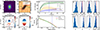 |
Fig. 1. Results from the 3D disk-halo decomposition applied to the mock MUSE cube of the simulated galaxy ID3. Panel (a): Mock MUSE white-light image with flux intensity contours overlaid. Panel (b): Position velocity diagram. The observed velocity profiles as measured with GALPAK3D and MPDAF (Bacon et al. 2016) are overlaid in red and green, respectively. The dotted black line shows the region beyond which the S/N of the emission line falls below unity, whereas the white contours show the flux intensity. Panels (c) and (d): Observed velocity field obtained using a traditional 2D line fitting code and the modelled velocity field obtained from 3D disk-halo decomposition with GALPAK3D. Panel (e): Contribution of the different components (stars-orange, gas-blue, DM-green curve) to the RC (dot-dashed curve; corrected for pressure support). Panel (f): Measured DM density profile (in green) compared to the true DM density profile (in red). The light shaded regions in these two panels show the 95% confidence interval. Panel (g): Posterior distributions (in blue) for a subset of the parameters we fit for: log(X) = log(M★/Mhalo), the virial velocity, the concentration, and the disk inclination. Panel (h): Posterior distributions for parameters derived from the fitted ones, including the DM density profile shape parameters α, β, and γ (computed using Eqs. (A.2), (A.3), and (A.4), respectively), as well as the stellar mass log(M★/M⊙). The recovered values are shown as the dark blue lines, while the values used as inputs for the simulation are shown as the red lines. |
Panels (c) and (d) of these figures show that the velocity fields modelled with our 3D disk-halo decomposition align well with the observed ones. Similarly, the modelled and observed velocity profiles (red and green curves, respectively, in panels (b) showing the position-velocity diagrams) closely match in regions where the S/N > 1. As illustrated, GALPAK3D allows us to probe low S/N regions in the galaxy outskirts, enabling more robust constraints on the outer-disk RC, compared to traditional 2D line fitting algorithms. Panels f) of Figs. 1 and 2 further demonstrate that our 3D disk-halo decomposition reliably recovers the true density profile within the uncertainties for both ID3 and ID982. Additionally, the recovered values of the fitted parameters (log X, vvir, cvir, and i – panels g) and the derived parameters (α, β, γ, and M★, panels f), indicated by the dark blue lines, all agree with the simulation input values, shown as the solid red lines, within 1σ. The most challenging parameter to recover is the halo concentration, cvir, which depends on estimating the virial radius, rvir, which lies well beyond the radial extent of the observed RC.
Overall, these results indicate that our 3D kinematic modelling framework provides reasonable estimates of galaxy physical parameters, even when kinematic coverage is limited.
4. Data: Intermediate-z SFGs
4.1. MUSE Hubble Ultra Deep Field
For this study, we exploited 3D spectroscopic observations from the MHUDF (Bacon et al. 2017, Bacon et al. 2023) to investigate the DM halo properties of intermediate-z SFGs which consists in three datasets: (1) the 3 × 3 arcmin2 mosaic of nine MUSE fields at a 10 h depth (MOSAIC); (2) a single 1 × 1 arcmin2 31 h depth field (UDF10), as well as (3) the 140 h MUSE eXtremely Deep Field (MXDF).
We made use of the publicly available catalogues and advanced data products, which can all be obtained from the AMUSED web interface9. In particular, we used the source files, which contain generic information related to the source (e.g. identifier, celestial coordinates, PSF model, and FWHM), images (e.g. white-light, narrow bands, HST images, and segmentation maps), and the MUSE data cubes centred at the source location which we used for our kinematic analysis
To prepare the data for the kinematic analysis, we truncated the sub-cubes in wavelength (with a width of 30 Å), centred on the emission line of interest using the spectroscopic redshifts, and subtracted the underlying continuum. No additional spectral or wavelength masking was applied.
We note that for some IFU sub-cubes, masks were applied during the kinematic fitting. Specifically, segmentation maps created with DS9 (Smithsonian Astrophysical Observatory 2000) were used in crowded regions where multiple galaxies at similar redshift appeared within the same sub-cube (∼13% of the sample). Pixels outside the target galaxy were set to NaN and excluded from the fits. No additional weighting was applied.
4.2. Sample selection
We used the MHUDFs main catalogue to select SFGs with z < 1.5 for our kinematic study, which have an effective signal to noise S/Neff > 10 for the brightest emission line (either [O II] λ3727, Hβ, [O II] λ5007, Hα). The effective S/N accounts for the fact that the surface brightness of the galaxy alone is not sufficient to determine the accuracy in the fitted disk structural and kinematic parameters, as the compactness of the galaxy with respect to the PSF also plays an important role (Bouché et al. 2015). The effective S/N is defined as
 (3)
(3)
where Re stands for the stellar half-light radius, RPSF = FWHM/2 is the radius of the MUSE PSF, and S/Nmax is the S/N of the emission line of interest in the brightest spaxel of the MUSE data cube centred on the galaxy. We also imposed Re/RPSF > 0.5 for our sample selection, to further avoid unresolved galaxies. Additionally, we only selected systems which have an inclination i > 30° for our kinematic study.
Figure 3 displays on the left the S/Neff, as a function of the S/N of the total line flux for the [O II] λ3726, λ3729, Hα, Hβ and [O III] λ5007 emitters from the MHUDF sample and on the right Re/RPSF as a function of the S/N of the brightest spaxel. From the whole MHUDF sample, 183 galaxies met the aforementioned selection criteria, namely S/Neff > 10, Re/RPSF > 0.5, and i > 30°.
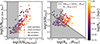 |
Fig. 3. Left: Effective S/N for the brightest emission line using Eq. (3), as a function of the S/N of the total line flux from the integrated spectrum. Right: Ratio of the stellar half-light radius to the PSF radius as a function of the S/N in the brightest spaxel. The grey shaded area in the panels marks the exclusion region, i.e. all galaxies with S/Neff < 10 and Re/RPSF < 0.5 are removed from the sample. The data points are colour-coded according to their half-light radii. The circles, stars, diamonds, and squares represent the [OII], Hα, Hβ, and [OIII] emitters, respectively. |
Moreover, we require our galaxies to be axisymmetric disks, i.e. unperturbed, in order to accurately model their morpho-kinematics and infer their DM halo properties. Therefore, we excluded merging systems from our sample. Additionally, we flagged galaxies, which show signs of gravitational interactions such as tidal arms; clumpy SF regions; as well as large residuals in the GALPAK3D fits, and plotted them with different symbols in the subsequent plots (the stars in all the figures denote the perturbed galaxies). This was done by visually inspecting the galaxies using the JWST and HST images, as well as investigating the catalogues from Ventou et al. (2019), who analysed the merger fraction in MUSE deep fields. This led to a sample of 173 galaxies.
Finally, for the disk-halo decomposition described in Sect. 2.2, we required the galaxies to be rotationally supported, therefore, we excluded dispersion-dominated systems from our analysis. Using the URC described in Sect. 2.1 to estimate the kinematics and shown in Fig. 6, we excluded galaxies with vmax/σ < 1, where σ = σ(2Re). The overall selection criterion results in a final sample of 127 intermediate-z main sequence galaxies that have S/Neff > 10, Re/RPSF > 0.5, inclinations i > 30°, and vmax/σ > 1.
4.3. Ancillary data
We also exploited the ancillary data available in the MHUDF area, namely the HST (Dickinson et al. 2003; Giavalisco et al. 2004; Grogin et al. 2011; Koekemoer et al. 2011) and JWST (Bunker et al. 2024; Eisenstein et al. 2026, 2025; Rieke et al. 2023; D’Eugenio et al. 2025; Williams et al. 2023a,b) images.
4.3.1. Morphology
For the stellar disk structural parameters, we used the F160W morphological analysis performed by van der Wel et al. (2012) with the GALFIT tool (Peng et al. 2010), providing the half-light radii (Re), Sersic index (n), axis ratios (b/a), and position angles (PA). We used the morphological parameters derived from the F160W band, as this is the reddest HST filter available and therefore best traces the underlying stellar mass distribution. The inclinations from this catalogue were used as priors in our dynamical modelling.
As already mentioned, the gas disk structural parameters yielded by GALPAK3D from the MUSE data are in good agreement with the ones derived for the stellar component from photometric observations for the vast majority of the SFGs analysed in this study. Similar results were found by Contini et al. (2016) and Bouché et al. (2022) for a subsample of the MHUDF galaxies.
4.3.2. SED
To obtain the stellar masses and SFRs, SED fitting was performed using the MUSE spectroscopic z and 11 HST broadband photometry measurements from the Rafelski et al. (2015) catalogue. The SED fits were carried out with the Magphys (da Cunha et al. 2015) software on the HST photometry using a Chabrier (2003) IMF, keeping the redshift fixed to the spectroscopic one, as well as with the Prospector SED fitting code (Johnson et al. 2021), observing good agreement between the results offered by the two different tools, with a scatter for log(M★/M ⊙ ) and SFRs in the order of ∼0.11 dex for our sample.
We note that in this study, we used the Magphys derived SFRs and M★, which assumed exponentially declining star formation histories (SFHs) with superimposed bursts. The SFRs correspond to the average SF over the last 0.1 Gyr, and as such are not very sensitive to short, intense bursts of SF.
4.3.3. Mass maps
We used all HST and JWST images available with a 30 mas pixel scale in the footprint of the MHUDF to produce high-resolution resolved stellar mass maps using the pixel-per-pixel SED fitting library pixSED10. The details are presented in Appendix D, and an example is shown in Fig. D.1.
As a first application, we used the mass maps for the whole sample to independently estimate the stellar disk component’s contribution to the disk-halo decomposition, employing the MGE method of Emsellem et al. (1994, see our Sect. 5.2.1 for more details).
As a second application, we used the stellar mass maps to estimate the bulge-to-total ratio (B/T) without relying on single-band observations, nor on the assumption of a constant mass-to-light ratio throughout the galaxies. To do so, we fitted the resolved mass maps using the AstroPhot package (Stone et al. 2023). First, we fitted a single Sérsic profile to the mass maps to estimate the centre position, ellipticity, and position angle of the galaxies. Then, we performed a second fit with a bulge-disk decomposition using the parameters from the first run as initial values for the disk component, where the disk was set to have a Sérsic index of n = 1 and the (circular) bulge was allowed to vary between n = 2 and n = 4. Furthermore, the bulge radius was constrained to be less than 3″, with an initial value of 0.5″, to force it to fit the inner parts of the galaxies. This analysis is relevant to our disk-halo modelling. For the 15 galaxies showing B/T > 0.2, we added a bulge component in the 3D disk-halo decomposition on the MUSE data, described in Sect. 2.2. It is also worth noting that the structural parameters recovered from the bulge-disk decomposition on the mass maps agree well with those from the van der Wel et al. (2012) catalogue.
4.4. Global properties of the sample
In this section, we present the physical properties of the galaxies that met our previously described selection criteria. Figure 4 shows the distribution of redshifts, stellar masss and Sérsic indices for our sample. The galaxies span redshifts between 0.28 < z < 1.49 (zmean = 0.85) and stellar masses 7.5 < log(M★/M⊙) < 11, with the distribution peaking around the mass regime where core formation is expected to be most efficient (e.g. Di Cintio et al. 2014, Tollet et al. 2016). Our sample contains disk galaxies with Sérsic indices peaking around n = 1, whereas only a few galaxies have n > 2.
 |
Fig. 4. Left: Histogram showing the redshift distribution of the MHUDF SFGs. Middle: Histogram showing the stellar mass distribution of sample (Bacon et al. 2023). Right: Histogram showing the distribution of the Sérsic indices (van der Wel et al. 2012). |
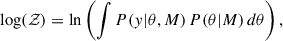
Figure 5 shows the stellar mass-SFR relation for the MHUDF sample. Both stellar masses and SFRs were measured from SED fitting, as described in Sect. 4.1. Most galaxies analysed in this study can be classified as star-forming main sequence (SFMS) galaxies, with only a subsample classified as starburst and/or in the process of quenching.
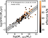 |
Fig. 5. Stellar mass – SFR relation for the MHUDF sample. The data points are colour-coded according to their effective S/N (Eq. (3)). The black line shows the star-forming main sequence at z = 0.85 (the mean redshift of our sample), as derived by Boogaard et al. (2018), whereas the grey shaded region shows the 0.44 dex scatter around the relation. The grey cross in the lower right corner indicates the median 1σ statistical uncertainties in M★ and SFR from Magphys. |
5. Results
In this section, we first test the six DM profiles and baryons-only model presented in Sect. 2.2 using a Bayesian analysis to identify which best describe the data (Sect. 5.1) and find that the DC14 profile is a good representation of the data. We then present the results from the 3D disk-halo decomposition using the DC14 DM profile (Sect. 5.2), and several cross-validation checks (Sects. 5.2.1–5.2.4). Finally, we present results on the DM fraction (Sect. 5.3), on the DM profiles and the core-cusp fractions (Sect. 5.4), on the stellar-halo mass relation (Sect. 5.5) on the concentration-mass relation (Sect. 5.6) and on concentration-density relation (Sect. 5.7).
Before discussing the disk-halo decomposition, we show in Fig. 6 examples of the 3D morpho-kinematic fits for three SFGs (ID 26, 6877, 958) with various S/N values ranging from ∼30 to ∼100 using the methodology described in Sect. 2.1. Additionally, the fluxes, S/N, velocities and velocity dispersions of the emission lines of interest in each spaxel of the MUSE cubes were also measured with a traditional 2D line fitting algorithm, CAMEL (Epinat et al. 2012). The position–velocity diagrams (PVs) shown in panel (f) of the figure were extracted from the MUSE cubes, with the PV slice taken along the kinematic major axis through the galaxy kinematic centre, using a 3-pixel-wide (0.6″) slit.
 |
Fig. 6. Example of morpho-kinematic maps for three galaxies, ID 26, 6877, and 958, covering the range of S/N ∼28 − 116. For each galaxy, the 11 panels show (a) the HST F160W image; (b) the emission-line flux map, with the S/N contours overlaid; (c+d) the observed velocity maps in [km/s] with the CAMEL (Epinat et al. 2012) and with GALPAK3D (URC), with the grey line showing the major-axis; (e) the observed velocity profile v⊥(r)sin(i)obs extracted along the major-axis; (f) the position-velocity diagram extracted along the major-axis; (g) the intrinsic velocity profile v⊥(r), i.e. corrected for inclination and instrumental effects; (h+i) the observed velocity dispersion maps in [km/s]; (j) the intrinsic velocity dispersion profile in [km/s]; and (k) the residuals map derived by computing the standard deviation along the wavelength axis of the normalised residual cube (see Bouché et al. 2022). In panels e, f, and g, the vertical dashed black line represents the radius at which the S/N ≃1, whereas the vertical dotted (light) green lines represent (3Re) 2Re. |
Figure 6 demonstrates that owing to our deep data with high S/N, both CAMEL and GALPAK3D enable us to probe the outer disk RCs, as illustrated in panels (e) by the (light) green dotted lines which show (3Re) 2Re. Nonetheless, GALPAK3D proves more effective at tracing the outer parts of the RC, as it exploits the full 3D information from all spaxels, including those with low S/N. In contrast, the CAMEL measurements tend to become increasingly uncertain at large radii, where the low S/N of individual spaxels leads to noisier and sometimes biased velocity estimates. This figure also shows that the disk kinematic 3D modelling reproduces the 3D data well, in some cases with very little residuals. These fits were used to select rotation-dominated systems in Sect. 4.2.
Next, we show in Figure 7 the RCs of the full sample, estimated with the URC model (Sect. 2.1). The left panel shows model RCs colour-coded by stellar mass, while the right panel plots the inner RC slope, S, against the stellar mass surface density. Both panels reveal the same trend: galaxies with higher stellar mass surface densities–typically more massive, brighter systems–exhibit steeper inner slopes, whereas lower-mass galaxies show shallower rises. The sample spans a wide variety of RC shapes, from rising to flat and even mildly declining at large radii, broadly consistent with trends observed in the local Universe (e.g. Persic et al. 1996, Katz et al. 2017, Li et al. 2020, Frosst et al. 2022).
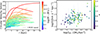 |
Fig. 7. Left: RCs (using the URC model, Sect. 2.1) of our sample of intermediate-z SFGs, colour-coded by stellar mass. The dotted black line shows the physical extent of 1 MUSE spaxel at z ∼ 1, namely 1.65 [kpc]. Right: Inner RC slopes, S (corrected for inclination), as a function of the stellar mass surface density. The data points are colour-coded according to their z. The error bars on the y-axis show the 95% confidence intervals from our 3D kinematic modelling, while the x-axis shows the 1σ uncertainties in ΣM★. |
In the remainder of this paper, we only present results obtained with the 3D disk-halo decomposition methodology presented in Sect. 2.2.
5.1. Model comparison and model selection
Using the 3D disk-halo decomposition methodology, we first identify which of the seven models–DC14, NFW, Burkert, Dekel-Zhao (DZ), Einasto, coreNFW, baryons-only–best describes the data by computing the Bayes factor for each pair of models. Namely, we use the model evidence log(𝒵) or marginal probability log P(y|M), defined as
 (4)
(4)
i.e. the integral of the posterior over the parameter space yielded by our MCMC fitting routine with pyMultiNest (Buchner et al. 2014). log(𝒵) serves as a measure of how well the model explains the observed data, accounting for both goodness of fit and model complexity. This metric is closely related to the Bayesian Information Criteria (BIC), which is BIC  where
where  is the maximum likelihood, k the number of parameters, and n the number of data points.
Following Kass & Raftery (1995), we rescale the evidence log(𝒵) by a factor of −2 so that it is on the same scale as the usual information criterion (BIC; deviance information criterion). We then compute the Bayes factor, defined as the ratio of the marginal probabilities of two competing models M1 versus M2,
 (5)
(5)
for each pair of models (e.g. Trotta 2008). Considering our scaling factor of −2 (see also Kass & Raftery 1995), positive evidence against the null hypothesis, i.e. that the two models are equivalent, occurs when the Bayes factor is > 3, whereas there is strong positive evidence against the null hypothesis when the Bayes factor > 20. This corresponds to a logarithmic difference Δ log(𝒵) of 2 and 6, respectively.
Before discussing the results for the entire sample, we present in Fig. E.1 the residual maps (generated from the residual cube as in Fig. 6) for each of the six DM profiles and the baryon only model for the same three galaxies from Fig. 6 and one extra galaxy from our sample. Alongside the maps, we report the Bayesian evidence (black text) and the Bayes factor (colour-coded as in Fig. 8) between DC14 and the competing models, and highlight the connection between the Bayes factor and the residual structure. We show that when the Bayes factor indicates strong positive evidence for a particular model, the corresponding residual map consistently exhibits lower residuals compared to the alternatives. We refer to Appendix E for more details.
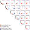 |
Fig. 8. Histograms showing the Bayes factor for all the pairs of halo models used in this study. The red columns show the number of galaxies that display a very strong positive evidence towards the first model, i.e. which have −103 < Δ log(𝒵) < −20. The two lighter red columns depict the number of galaxies that show strong positive evidence and positive evidence for the first model, i.e. which have −20 < Δ log(𝒵) < −6 and −6 < Δ log(𝒵) < −2, respectively. The blue columns show the number of galaxies that show very strong positive evidence for the second model, i.e. 20 < Δ log(𝒵) < 103, while the lighter blue columns display the number of systems that show strong positive evidence and positive evidence for the second model, namely 6 < Δ log(𝒵) < 20 and 2 < Δ log(𝒵) < 6, respectively. The grey columns display the number of galaxies for which both models perform similarly, having −2 < Δ log(𝒵) < 2. In each panel, model 1 refers to the first model listed in the title, while model 2 refers to the second model. |
Regarding the entire sample, Fig. 8 shows Δlog(𝒵) for all the DM model pairs where the red (blue) bars show the number of galaxies that display strong evidence for (against) the first model, while the grey bars correspond to the number of galaxies for which the two models are equivalent. The first panel of this figure indicates that, compared to NFW, DC14 provides fits that are equally good or better in ∼90% of the sample, broadly consistent with the trends reported by Katz et al. (2017) for the SPARC sample.
Similarly, the first row shows that, compared to Burkert, Dekel-Zhao, Einasto, coreNFW, and baryon-only models, DC14 performs at least as well as or better in 81%, 84%, 82%, 88%, and 96% of the sample, respectively (see Table 2 for details). Taken together, these comparisons suggest that DC14 is among the profiles that best represent the data, performing comparably to the Dekel-Zhao and Einasto models. This is in line with earlier findings, such as those of Li et al. (2019), who showed that cored profiles like DC14 and Einasto can provide better fits than cuspy NFW models for the local SPARC sample.
Comparison of DM halo models for the whole sample.
Figure 8 reveals that for many galaxies (≈10–50%) in our sample, the two models under consideration are statistically equivalent, i.e. fit the data similarly well (grey bars in Fig. 8). In order to understand whether the S/N of the data played a role, we repeated this analysis using only systems which have S/Neff > 50 (44 galaxies) and found that the number of galaxies for which the two models are indistinguishable decreases below 20% in most cases (see Table 3 for more details). We found that the DC14 model tends to describe the kinematics of the high S/N data better than the alternatives.
Comparison of DM halo models for high S/N galaxies.
For the baryon-only model, the last column of Fig. 8 shows that it generally performs less well than models that include a DM halo. In addition, the baryon-only model yields dynamically inferred disk masses (M★ + Mmol) that are systematically higher than the stellar masses derived from SED fitting. After accounting for molecular gas using scaling relations (e.g. Freundlich et al. 2019; Tacconi et al. 2020), we find that the baryon-only model still overpredicts stellar masses by ∼0.76 dex (for a Chabrier IMF) or ∼0.53 dex (for a Salpeter IMF), with offsets up to ∼1 dex in some cases (plots not shown). These offsets confirm that even when adopting a heavier IMF, the baryon-only model cannot reconcile the observed kinematics with the SED-inferred stellar masses. Furthermore, the typical uncertainties in SED-inferred stellar masses due to variations in modelling assumptions–such as SFH, dust, metallicity, and IMF–are estimated to be in the range of 0.2–0.3 dex at maximum (e.g. Mobasher et al. 2015), which is below the magnitude of the observed offset in our sample. In contrast, the DC14 model yields dynamically inferred disk masses that agree well with the SED-based estimates (see Sect. 5.2.3 for details). The challenges we find in reconciling baryon-only models with both kinematic and SED-based constraints are in line with earlier results such as those of Bershady et al. (2011), who suggested that disk galaxies are typically not maximal, especially in the mass range probed here.
To conclude, our analysis suggests that the DC14 density profile (Eq. (15)) provides, on average, a better description of the kinematics of intermediate-z SFGs than the other profiles considered, with the Dekel-Zhao and Einasto models also performing comparably well, while baryon-only models are broadly disfavoured with respect to models which include a DM component. In the remainder of the paper, we show results obtained with the DC14 halo model (see Appendices F, G, and H for the results inferred using all six DM halo models).
5.2. 3D disk–halo decompositions
Figure 9 shows the results from the 3D disk-halo decompositions for the same three galaxies shown in Fig. 6 using the DC14 DM halo profile (Eqs. (A.1)–(A.4)). All velocities are intrinsic, i.e. corrected for inclination and instrumental effects, including seeing. This figure shows that the RCs are dominated by the DM component. Consequently, it is worth noting that the RC data contains information on the halo shape parameters (α(X),β(X),γ(X)), which in turn, yields a constrain on the ratio Mdisk/Mvir for DC14 DM profiles. As a result, this breaks the traditional disk-halo degeneracy.
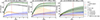 |
Fig. 9. Examples of the 3D disk-halo decomposition for the three galaxies show in Fig. 6 using a DC14 DM profile (Eq. (A.1)). The solid black line represents the rotational velocity v⊥(r). The thick dashed black line represents the circular velocity vc(r), i.e. v⊥(r) corrected for pressure support (Sect. 2.2). The green curve represents the RC of the DM component. The solid orange and blue curves represent the disk and H I components, respectively. The light shaded regions show the 95% confidence intervals. The dotted brown lines represent the stellar component obtained using the MGE modelling of the stellar mass maps (see Sect. 5.2.1). All velocities are intrinsic, i.e. corrected for inclination and instrumental effects, including seeing (PSF). The black dotted line shows the physical extent of a MUSE spaxel, the dot-dashed red line shows 2 × Re, while the dashed grey line shows the region beyond which S/N < 1. |
Before discussing the results on the DC14 profiles, we perform several cross-checks of our 3D disk-halo decomposition. We first compare (Sect. 5.2.1) our disk component to the one obtained from the stellar maps derived from HST and JWST photometry (described in Appendix D). We then perform 1D disk-halo decomposition (Sect. 5.2.2) from external data using the stellar surface brightness and several H I profiles. Finally, we perform some self-consistency checks (Sects. 5.2.3–5.2.4) for DC14.
5.2.1. Stellar gravitational field from mass maps
To estimate the stellar disk contribution to the disk–halo decomposition, we applied the MGE method (Monnet et al. 1992, Emsellem et al. 1994) to the stellar mass maps derived from pixel SED fitting (Appendix D). This was done using the mgefit Python package of Cappellari (2002), and we considered the PSF when fitting the 2D stellar maps. Each MGE model comprises concentric 2D Gaussians characterised by peak intensity, dispersion, and axial ratio or flattening11. Finally, based on the MGE parameters, we used the mge-vcirc module from the jampy Python package of Cappellari (2008), to calculate the gravitational acceleration (v2/r) in the equatorial plane of each galaxy. This approach models the mass distribution using an MGE representation directly from the mass maps, under the assumption of dynamical equilibrium (thereby eliminating the need to assume a constant mass-to-light ratio as is typically required when performing MGE modelling on galaxy images).
While the ancillary imaging used to derive the mass maps includes long-wavelength coverage that helps mitigate uncertainties due to dust attenuation, we note that stellar masses derived from SED fitting can still be subject to systematic uncertainties of up to ∼0.3 dex (e.g. Mobasher et al. 2015). Such uncertainties propagate into the stellar mass maps, and therefore into the inferred stellar circular velocities.
With these limitations in mind, we show in Fig. 9, as the dotted brown curves, the predicted circular velocity of the stellar mass distribution, as derived from the mass maps. As this figure demonstrates, there is good agreement between the v★(r) determined from the mass maps and the MUSE data. For approximately 80% of the galaxies in our sample, the RCs obtained from the two methods agree within the errors. Moreover, the half-light radii and surface brightness profiles from the mass maps are very similar to those obtained from the ionised gas tracers.
Discrepancies in the order of ∼10–20 km/s, where present, are mostly confined to the central regions, and remain within the uncertainties of the GALPAK3D velocities (yellow shaded regions in Fig. 9). These central differences likely arise from the sensitivity of the MGE method to the precise PSF modelling.
Crucially, the agreement between the MGE-based and GALPAK3D stellar circular velocities for the majority of the sample provides an independent validation of our disk-halo decomposition. While GALPAK3D assumes an Sérsic disk profile, the MGE approach does not impose a parametric form on the stellar mass distribution. The fact that both methods yield broadly consistent stellar contributions implies that the stars in our sample galaxies are indeed in (near) equilibrium disks. The results obtained in this section were used as a qualitative check against the results obtained with our 3D parametric modelling.
5.2.2. Cross-checks with 1D disk–halo decomposition
To independently perform the disk–halo decomposition from the observed RC, we computed the expected baryonic contribution by solving the Poisson equation for arbitrary surface density distributions (i.e. solving Eq. (4) of Casertano 1983) using the vcdisk tool12, assuming a vertical structure of the disk as in Sect. 2.2. For the disk component, vdisk(r), we used a Sérsic surface brightness profile with parameters derived from the HST/F160W data (van der Wel et al. 2012, see Sect. 4.3), assuming a constant mass-to-light ratio. For the H I component, we used the radial profiles from Martinsson et al. (2016) or from Wang et al. (2025), where the H I masses were inferred from the stellar masses of our sample using the z ∼ 1 MH I − M★ scaling relation of Chowdhury et al. (2022, their Eq. (1)).
The purple curves in Fig. 10 show the resulting DM velocity curves derived using Eq. (1), i.e. by subtracting the baryonic components computed with vcdisk from the total measured vc from MUSE, for the same three galaxies shown in Fig. 9. For the examples shown here, we used the Wang et al. (2025) H I profile for the gas component; we note, however, that using the Martinsson et al. (2016) profile leads to similar results. The GALPAK3D-based velocity curves, shown in green, assumed a DC14 DM halo. As illustrated in Fig. 10, the 1D and 3D decompositions agree within the uncertainties. We find consistent DM contributions between the two methods for ∼87% of the galaxies in our sample. The discrepancy, when present, mostly occurs for the perturbed, as well as for compact, low S/Neff galaxies.
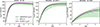 |
Fig. 10. Comparison of DM velocity profiles for the three galaxies shown in Fig. 9. The green curves show the profiles modelled with GALPAK3D assuming a DC14 halo, while the purple curves are obtained by subtracting the baryonic contributions obtained with vcdisk from the MUSE-derived vc(r). The green shaded regions indicate the 95% confidence intervals from the 3D disk–halo decomposition fits. |
5.2.3. Self-consistency checks for DC14
In this section, we check for consistency between the M★ yielded by our 3D disk-halo decomposition and M★ derived from SED fitting. We recall that the stellar mass was a free parameter (contained in X) in our disk-halo decomposition using DC14 and the disk-halo degeneracy is broken because (i) the RC shape is driven by the shape parameters which depends on X ≡ log(M★/Mvir), and (ii) the RC also yields vvir from the maximum velocity.
Figure 11 (left) shows the comparison between the kinematically inferred and SED-based stellar masses. The majority of galaxies lie within a < ± 0.5 dex region (grey shaded area) around the one-to-one relation (dashed line), indicating general agreement between the two estimates. The mean offset is modest, with dynamically inferred stellar masses being on average 0.11 dex lower than the SED-based stellar masses. The largest discrepancies between SED and kinematic-based M★ occur for the perturbed galaxies as well as for compact, low S/Neff galaxies. Excluding the perturbed galaxies and performing a linear fit to the data yields a slope of ∼0.82 ± 0.1, which is close to the expected slope of 1 for the relation between M★ from SED fitting and M★ from the kinematic analysis. Overall, this figure demonstrates that our disk-halo decomposition produces stellar masses broadly consistent with those derived from SED fitting.
 |
Fig. 11. Left: Comparison between the stellar masses inferred from our disk-halo decomposition using the DC14 halo model and the stellar masses inferred from photometric observations. The dashed black line shows the 1:1 relation, and the grey shaded region shows the 0.5 dex dispersion around the relation. The data points are colour-coded according to their S/Neff. Right: DM inner slope, γ, as inferred from the DC14 halo model as a function of the stellar masses derived from SED fitting. The data points are colour-coded according to their virial masses. The coloured curves depict the parametrisation of Di Cintio et al. (2014) for γ (Eq. (A.4)), for four different virial masses, as indicated in the legend. In both panels, the circles show the regular MHUDF galaxies, while the stars depict the perturbed galaxies from our sample. The error bars represent the 95% confidence intervals. |
5.2.4. Cross-validation check for DC14
In an attempt to independently verify the DC14 framework of varying inner DM slopes with mass, we show in Fig. 11 (right) the inner DM slope, γ, as a function of the stellar mass inferred from SED fitting (i.e. independent of our GALPAK3D fits) with the data points colour coded according to their virial masses obtained from the 3D kinematic modelling. This figure indicates that the DM slopes (γ values) we infer using GALPAK3D agree well with the DC14 expectations for the respective masses.
5.3. DM fractions
In this section, we investigate the DM fraction, fDM(< Re), of our sample by integrating the DM and disk mass profile to Re. Figure 12 shows fDM(< Re), as a function of the stellar mass surface density. Additionally, we also plot in this figure the DM fractions obtained by Puglisi et al. (2023) for SFGs at z ∼ 1.5, as well as the DM fractions inferred by Genzel et al. (2020) and Nestor Shachar et al. (2023) for SFGs at z = 1 − 2 with black symbols. We find that 89% of our sample has fDM(< Re) > 50%.
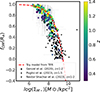 |
Fig. 12. DM fractions within Re as a function of the stellar mass surface density. The black diamonds show the DM fractions inferred by Puglisi et al. (2023) for z ∼ 1.5 SFGs, the black squares depict the z = 1 − 2 sample of Genzel et al. (2020), while the black triangles show the RC100 sample from Nestor Shachar et al. (2023). Our sample is colour-coded according to its redshifts. The circles depict the regular galaxies, while the stars represent the perturbed systems from our sample. The error bars represent the 95% confidence intervals. The red dotted line shows the toy model derived from the Tully–Fisher relation (see Bouché et al. 2022, Sect. 5.1). |
For a given stellar mass surface density, ΣM★, we infer fDM(< Re) for the MHUDF galaxies, consistent with those reported by Puglisi et al. (2023), Genzel et al. (2020) and Nestor Shachar et al. (2023) for their samples. However, compared to the SFGs analysed in the three aforementioned studies, our sample extends to the lower-mass regime, and, thus, to lower mass surface densities  . As this figure illustrates, the galaxies follow a relatively tight relation in the fDM(< Re)–ΣM★ plane, consistent with Genzel et al. (2020), Puglisi et al. (2023), Nestor Shachar et al. (2023). This trend likely reflects the underlying Tully–Fisher relation for disks (e.g. Übler et al. 2017), as illustrated by the simple toy model at z ∼ 1 (red dotted line; see Bouché et al. 2022, Sect. 5.1).
5.4. DM density profiles and inner slopes
In this section, we discuss the DM inner slopes, γ, of our sample. The three panels of Fig. 13 show the density profiles for the same three galaxies presented in Fig. 9. The inferred γ values are reported in the upper right corner of each panel. From left to right, the profiles become progressively more cored, as illustrated by the overall flattening of the central density. The dashed vertical line marks the physical scale of a single MUSE spaxel. Although MUSE’s spatial resolution limits direct probing of the inner ≲1–2 kpc, the global curvature of the RC over several kiloparsecs retains information on the central DM slope: cored profiles produce a shallower rise compared to cuspy ones, and this distinction remains observable at MUSE resolution (Fig. 9). The robustness of our slope measurements is further supported by tests on mock MUSE cubes (Sect. 3). These tests demonstrate that the inferred γ values recover the true input slopes within 1σ.
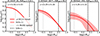 |
Fig. 13. Example of DM density profiles for the same three galaxies shown in Fig. 9. The y-axis shows the DM density, ρDM(r), in units of M⊙/kpc3, and the x-axis the r/Re. The red curve shows the DM density profile obtained using the DC14 halo model, whereas the red-shaded region represents the 95% confidence interval. The inferred DM inner slopes, γ, are indicated in the upper left corner of each panel. The vertical dashed black lines represent the 0.2″ spaxel scale, indicating the lower limit of our constraints. |
Globally, our analysis reveals that ∼66% of our sample of intermediate-z SFGs exhibits cored DM profiles, with γ < 0.5. We note that observational evidence exists for DM cores up to z ∼ 2 (e.g. Genzel et al. 2017; Sharma et al. 2022; Nestor Shachar et al. 2023), and possibly as far as z ∼ 6 (Danhaive et al. 2026). We discuss these findings further in Sect 6.1.
5.5. Stellar–halo mass relation
The M★ − Mvir relation in the ΛCDM framework is a well-known scaling relation describing the relationship between the mass of a DM halo and the stellar mass of the galaxies residing within it. This scaling relation reflects the SF efficiency, and thus the efficiency of feedback processes, providing crucial insights into galaxy formation models (e.g. Vale & Ostriker 2004, Moster et al. 2010). Several recent studies have investigated the stellar mass–halo mass relation using RCs of individual galaxies (e.g. Read et al. 2017, Di Paolo et al. 2019, Posti et al. 2019, Li et al. 2020, Romeo et al. 2023, Mancera Piña et al. 2026), generally finding a considerable scatter in the relation.
Figure F.1 shows the stellar mass–halo mass relation for our sample. We show the SED-based stellar masses versus the virial masses, as inferred from the 3D disk-halo decomposition, using all the different halo models. The upper left panel shows the DC14 results, which yield the tightest M★ − Mvir relation amongst all the tested halo models. We find that our results are qualitatively in good agreement with the relation inferred by Behroozi et al. (2019), as well as the one derived by Girelli et al. (2020) using the (sub)halo abundance matching technique, albeit with a larger scatter. The latter two studies quote a scatter in the M★ − Mvir relation of about ∼0.2 − 0.4 dex, which is much smaller than the scatter ≳1.5 dex we measure for the MHUDF galaxies. Similar results were found by Li et al. (2020) for the local SPARC sample, using DC14 without ΛCDM priors. It is also worth noting that our sample does not probe the high-mass end, and therefore does not reach the bend in the M★ − Mvir relations. In Appendix F we further discuss the results obtained with the other halo models.
5.6. Concentration–halo mass relation
A fundamental prediction of N-body ΛCDM simulations is the concentration of DM halos, cvir ≡ rvir/rs, which encodes the assembly history of the halo. The concentration is expected to decrease with increasing halo mass and redshift, following  and cvir ∝ (1 + z)−1 (Bullock et al. 2001); weh, as a consequence of the redshift evolution of the virial radius rvir. The cvir–Mvir relation has been tested using RCs in the local Universe (e.g. Allaert et al. 2017; Katz et al. 2017; Li et al. 2020), but remains poorly constrained at higher redshifts for galaxy-scale halos (e.g. Bouché et al. 2022; Sharma et al. 2022), and has been primarily probed at the high-mass end using galaxy clusters (e.g. Biviano et al. 2017).
Figure 14 (left) shows the concentration–halo mass relation for our sample. The solid coloured lines and shaded regions show the cvir − Mvir relation and scatter of 0.11 dex, respectively, from Dutton & Macció (2014) for simulated halos with 0.3 < z < 1.5. The MHUDF galaxies show significant scatter around the expected scaling relations. This is expected, as even DM–only simulations produce considerable intrinsic scatter (e.g. Correa et al. 2015), and baryonic processes are known to further increase the scatter (e.g. Sorini et al. 2025). We quantify the agreement with the theoretical relation by accounting for both measurement uncertainties and the intrinsic 0.11 dex scatter in the cvir–Mvir relation. Approximately 70% of the MHUDF galaxies lie within 1σ of the Dutton & Macció (2014) relation at their respective redshifts, a level of agreement broadly consistent with that observed in the local z = 0 SPARC sample (Li et al. 2020), when no ΛCDM priors are used in the modelling. For completeness, we show in Fig. G.1 the cvir − Mvir relation inferred from all six different halo models described in Appendix A.
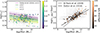 |
Fig. 14. Left: Concentration–halo mass relation for the MHUDF sample. The solid coloured lines show the cvir − Mvir relation from Dutton & Macció (2014) for 0.3 < z < 1.5, while the shaded regions show the 0.11 dex scatter around the relations. The data points are colour-coded according to their redshifts. Right: rs, DMO = rvir/cvir in [kpc] as a function of the halo masses. The dotted black line displays the observed scaling relation for z = 0 low surface brightness systems inferred by Di Paolo et al. (2019), while the solid black line shows the predictions from Dutton & Macció (2014). The data points are colour-coded according to their effective S/N. In both panels, the circles show the regular MHUDF galaxies, while the stars depict the perturbed galaxies. The error bars represent the 95% confidence intervals. |
Figure 14 (right) shows the scaling relation between the halo mass, Mvir, and the scale radius,  , which is a redshift-independent parameter (e.g. Bullock et al. 2001, Dutton & Macció 2014). The sample follows a tighter sequence in the rs, DMO − Mvir than in the cvir − Mvir plane. However, we observe a small systematic offset: our sample tends to have larger rs,DMO values at fixed Mvir than predicted by simulations or inferred observationally for the low surface brightness sample of Di Paolo et al. (2019). This offset likely arises from the uncertainties in estimating rvir, which requires extrapolation beyond the radial extent of the observed RCs. Since rvir is not directly measured but inferred by fitting halo models over a limited kinematic range, this extrapolation introduces significant model-dependent uncertainties. As a consequence, derived parameters such as cvir and rs,DMO are less tightly constrained than for local galaxies, where extended HI RCs provide direct measurements out to large radii.
5.7. Concentration-density relation
The cvir − Mvir or rs − Mvir relations can be recast to the rs − ρs relation. Figure 15 shows this relation for the MHUDF galaxies in panel (a). We observationally confirm the well-known anti-correlation between rs and ρs with a slope of ≈ − 1 (e.g. Salucci & Burkert 2000, Spano et al. 2008, Kormendy & Freeman 2016), consistent with expectations from hierarchical clustering of DM halos (e.g. Gott & Rees 1975). Using HyperFit (Robotham & Obreschkow 2015), we fit a power-law model of the form ρs ∝ rsx(1 + z)y, accounting for the errors. Before exploring a possible redshift evolution, we assessed the completeness of our sample. While the MHUDF survey is complete down to log(M★/M⊙) = 8.61 for 0.2 < z < 1.5, our stricter S/N cuts imply completeness only above log(M★/M⊙) = 8.8. We therefore adopt this mass limit, excluding 22 galaxies from our fit. Restricting to this complete sample, we find  (purple line in Fig. 15a). For comparison, Djorgovski (1992) showed that the density of DM halos, ρ, and the size, r, follow ρ ∝ r−3(3 + n)/(5 + n). The rs slope of ∼ − 1.03 that we infer yields n ∼ −1.92. This value for n is very close to n ∼ −2 expected in ΛCDM for halo masses of ∼1012 M⊙ (e.g. Shapiro & Iliev 2002). The redshift term from the fit suggests a mild increase of ρs with z, consistent with higher-z galaxies lying above the local relation (dashed red and black lines in panel a). While this points towards denser halos at earlier epochs, a larger sample is required to confidently confirm this trend.
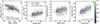 |
Fig. 15. Panel (a): Halo scale radius–DM density relation for the MHUDF sample. The dashed black line shows the relation inferred by Di Paolo et al. (2019) for z = 0 low surface brightness galaxies, while the dashed red line shows the relation derived by Kormendy & Freeman (2016) for z = 0 SFGs. The purple line shows a power-law fit to our mass complete sample, with |


Next, we show in panels (b), (c), and (d) the halo structural parameters versus the stellar masses for our intermediate-z (coloured data-points) and the SPARC z = 0 galaxies (grey diamonds, Li et al. 2020). Panel (b) shows rs–M★ relation, panel (c) the ρs–M★ relation, and panel (d) the halo surface density Σs(=ρsrs)–M★ relation. Consistent with Li et al. (2019), we find that rs and Σs increase with M★, while ρs remains roughly constant. This implies that more massive galaxies inhabit progressively larger halos, with the mass and size growing in tandem to maintain a nearly constant density. The observed increase of Σs with M★ agrees with Zhou et al. (2020, SPARC) and Kaneda et al. (2024, theory). In contrast, Donato et al. (2009) and Kormendy & Freeman (2016) found ΣDM to be constant with stellar mass. These discrepancies likely stem from differing halo models and fitting methods. While Kormendy & Freeman (2016) used maximum-disk fits with pseudo-isothermal halos, where ρ0 is the central density and rc the core radius, we use ρs and rs from DC14 profile. For example, Li et al. (2019) shows that adopting Kormendy’s assumptions for SPARC indeed yields a constant ΣDM, but argues that the maximum-disk method is unsuitable for low- and intermediate-mass galaxies, as it artificially boosts the stellar contribution at the expense of the halo.
From direct comparison of linear fits in panels (b), (c), and (d) (MHUDF -purple line; SPARC -grey line), we find that our intermediate-z galaxies have rs consistent with the local sample. This observational result is in line with DM-only simulations showing rs to be nearly redshift-invariant (e.g. Bullock et al. 2001; Dutton & Macció 2014). In contrast, ρs appears ∼0.3 dex higher at intermediate z than locally, suggesting denser halos at earlier epochs, consistent with the mild redshift dependence inferred from the fit in panel a). The tentative redshift dependence of ρs is in qualitative agreement with theoretical expectations (e.g. Zhao et al. 2003, 2009, see Fig. 20 of the latter paper). Such a trend arises naturally from the physics of hierarchical structure formation in an expanding Universe. At higher z, the mean background density is higher, and since the characteristic density is related to the density of the Universe at the time of halo collapse, halos forming at earlier epochs tend to have higher densities.
6. Discussion
6.1. Core formation
In Sect. 5.4, we find that ∼66% of the intermediate-z SFGs from our sample have cored DM density profiles. Within ΛCDM, baryon – DM interactions in the inner halo – driven by AGN feedback (Dekel et al. 2021), infalling gas clumps (El-Zant et al. 2001; Romano-Díaz et al. 2008; Johansson et al. 2009), central stellar bars (Weinberg & Katz 2002), or stellar feedback (Read & Gilmore 2005; Governato et al. 2010; Teyssier et al. 2013; Brooks & Zolotov 2014; Di Cintio et al. 2014; Tollet et al. 2016; Bose et al. 2019; Freundlich et al. 2020b; Jackson et al. 2024; Azartash-Namin et al. 2024) – have been proposed as core-forming mechanisms. Most of these studies find that feedback can induce core formation, with the efficiency of this process depending on the stellar-to-halo mass ratio (e.g. Di Cintio et al. 2014; Tollet et al. 2016; Lazar et al. 2020; Azartash-Namin et al. 2024), while Bose et al. (2019) find no such correlations in the APOSTLE and AURIGA simulations. If stellar feedback-induced core-formation is currently the favourite mechanism, very few authors report direct observational evidence linking cores to SFHs or SFRs (e.g. Read et al. 2019; Bouché et al. 2022).
Motivated by these studies, we investigated whether the presence of DM cores in our sample correlates with the current SF activity, quantified either by the offset from the SFMS or by the specific SFR (sSFR = SFR/M★). Figure 16a shows the MHUDF galaxies with log(M★/M⊙) > 8.5 in the ΔMS–M★ plane, colour-coded by their inner DM slopes. We find no evidence for a correlation between γ and ΔMS: both cored and cuspy systems exhibit a wide range of SFRs. Figure 16b shows the DM density within 150 pc as a function of the stellar-to-halo mass ratio, with the data points colour-coded by their sSFRs. Again, we find no correlation between ρDM(150 pc) and the sSFR. Overall, our results indicate no link between the central DM density and the current level of SF activity in these intermediate-z galaxies.
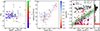 |
Fig. 16. Panel (a): Stellar masses of the entire MHUDF sample (with log(M★/M⊙) > 8.5) as a function of the offset from the SFMS (ΔMS) from Boogaard et al. (2018). The data points are colour-coded according to the DM inner slope, γ. The error bars show the 1σ statistical uncertainties in M★ and SFR from Magphys. Panel (b): DM density at 150 pc as a function of log(M★/Mvir). The data points are colour-coded according to their sSFRs. The error bars represent the 95% confidence intervals from our disk-halo decomposition. In both panels, the circles show the regular MHUDF galaxies, while the stars depict the perturbed systems from our sample. Panel (c): γ as a function of the stellar masses for the mass-matched MHUDF sample (red circles) and the TNG galaxies (black open squares, from Pillepich et al. 2019). The large indigo data points show the mean values for γ of the MHUDF sample in 6 mass bins, while the grey diamonds show the mean values for the mass-matched SPARC sample at z = 0 (using the DC14 fits without ΛCDM priors from Li et al. 2020). The green curve shows the predictions from Tollet et al. (2016) at z = 0, whereas the green shaded region shows the 0.18 dex scatter around the relation. The histogram shows the distribution of the γ values for the mass-matched MHUDF (in red), SPARC (in grey), TNG (in black), and NIHAO (in green) samples. |
We note, however, that this lack of a correlation with current, integrated SF activity is not unexpected, since (i) models predict that core formation is driven by repeated, rapid fluctuations in the gravitational potential, triggered by bursts of SF and gas outflows, rather than by the instantaneous SFR (e.g. Pontzen & Governato 2012) and (ii) the integrated SFRs used here are not by themselves sensitive to bursty SFHs, limiting their diagnostic power. Testing for the feedback-induced core-formation scenario requires full SFHs, as in Read et al. (2019), which we defer to future work.
On the other hand, γ seems to be strongly dependent on the galaxy mass. Figure 16a already indicates that γ is correlated with M★, and Fig. 16c shows the γ − M★ relation for the MHUDF galaxies.
To place our results in a broader context, Fig. 16c compares the MHUDF sample (red circles and red histogram; indigo circles showing the mean γ values in six mass bins), to the z = 0 SPARC galaxies (grey diamonds representing the mean γ values in six mass bins and grey histogram; using the DC14 fits from Li et al. 2020), and the z ∼ 1 TNG50 SFGs (black open squares and black histogram; Pillepich et al. 2019). The green curve shows the z = 0 predictions from the NIHAO hydrodynamical simulation (Tollet et al. 2016), while the green histogram shows the distribution of the gamma values of individual NIHAO SFGs. To ensure a meaningful comparison, all datasets are restricted to the same stellar-mass range, 8.5 < log(M★/M⊙) < 10.5.
As this panel illustrates, the TNG50 SFGs are almost exclusively cuspy, suggesting that TNG50 may not fully capture baryonic core-formation processes, at least for the mass and z range probed in this work. In contrast, hydrodynamical simulations such as NIHAO predict a strong mass dependence of the inner slope that is in broad agreement with our observational results and those from Li et al. (2020). We note that the MHUDF galaxies with γ ∼ 0.25 across a broad M★ range can be explained by the intrinsic scatter of ∼0.25 dex in the stellar-to-halo mass relation (Behroozi et al. 2019) and the lack of scatter in the γ − log(X) relations used from DC14.
6.2. Model limitations and caveats
Performing a disk-halo decomposition at intermediate z when the resolution or beam is comparable to the galaxy radius is challenging, but performing 3D forward modelling over several thousands of spaxels is possible provided that (i) the PSF and LSF are both stable and well characterised, and (ii) sufficient S/N is available. For illustration purposes, a galaxy with a Gaussian profile convolved by a Gaussian beam yields a Gaussian whose FWHM is  . Provided there is sufficient S/N, one can recover the galaxy intrinsic morphological parameters FWHMint as discussed in Bouché et al. (2015, 2021) and in Refregier et al. (2012) in the context of weak lensing. The same principle applies to 3D data.
Rotation curve decompositions in lower-mass galaxies M★ < 1010 M⊙ are somewhat easier given that the DM fraction increases in galaxies with lower mass or lower surface brightness. Hence, the RCs are more dominated by the DM component than in high-mass galaxies. This implies that information on the DM profile is contained in the shape and curvature of the RCs. For instance, a DM core of a few kiloparsecs in ρ(r) is felt over several kiloparsecs in the RCs, given that the rotation velocity is driven by the cumulative mass profile v(r)2 ∝ GM(< r)/r (where the transition radius rs is > 10 kpc).
Performing a disk–halo decomposition at intermediate redshifts is certainly challenging. In Sect. 3, we tested our 3D disk–halo decomposition method on mock data cubes generated from realistic simulations with disk and DM properties similar to our galaxies. We also carried out additional tests and self-consistency checks (Sect. 5.2), which indicate that our methodology remains robust despite assumptions and approximations that may not hold for all the galaxies in our sample. We also examined whether the adopted baryonic parametrisation and priors introduce systematic biases in the inferred halo properties, and find that their impact is generally small. Nonetheless, some limitations remain.
First, we assumed purely circular motions in axisymmetric disks, neglecting non-circular components. Non-circular motions – such as inflows, outflows, or bars – can bias RC measurements and mimic a more cored distribution (e.g. Oman et al. 2019; Marasco et al. 2018). Based on our MGE modelling of the mass maps and JWST imaging, we find no strong evidence for barred galaxies in our sample, although we cannot fully rule out the presence of weak non-circular motions. These remain difficult to model even in the local Universe (e.g. Di Teodoro & Peek 2021), and their treatment becomes even more challenging at higher redshifts (e.g. Genzel et al. 2023). We defer the analysis of non-circular motion to another paper.
Second, due to the lack of resolved H I data at intermediate z, we adopted a constant surface density or the mean surface density profiles derived from observations of local SFGs for the H I contribution. Contrary to the vast majority of the kinematic studies at z > 0, we include and marginalise over an H I component and show that different plausible assumptions (a constant ΣH I, or the profiles proposed by Martinsson et al. 2016; Wang et al. 2025) yield consistent results (see Appendix B). However, the true diversity of H I surface density profiles at z ∼ 1 may deviate from the mean, which may affect the accuracy of the inferred mass distribution. Using vcdisk, we estimate such deviations to be ∼10–15 km/s, well within our velocity uncertainties. We therefore conclude that our results are robust against reasonable variations in H I profiles. Looking ahead, facilities such as the Square Kilometre Array (SKA) will deliver spatially resolved H I measurements at z > 0, allowing a more accurate characterisation of atomic gas density profiles and, in turn, more robust disk–halo decompositions of intermediate-z SFGs, in line with what is currently achievable only in the local Universe.
7. Summary and conclusion
In this paper we analysed the DM halo properties of a large sample of 127 SFGs, spanning a wide redshift (0.28 < z < 1.49) and stellar mass (8 < log(M★/M⊙) < 11) range. To do so, we used deep MUSE IFU observations from the MHUDF survey (Bacon et al. 2023). We performed a disk–halo decomposition using a 3D forward modelling approach that accounts for stellar, gas, DM, and (where applicable) bulge components, including corrections for pressure support. For the DM component, we tested six different density profiles: (1) the DC14 profile (Di Cintio et al. 2014), linking the DM profile shape to the stellar mass–halo mass ratio; (2) NFW (Navarro et al. 1997); (3) Burkert (Burkert 1995); (4) Dekel-Zhao (Freundlich et al. 2020b); (5) Einasto (Navarro et al. 2004); and (6) coreNFW (Read et al. 2016), as well as baryon-only models. The robustness of our methodology was assessed through application to mock MUSE data generated from idealised disk simulations and through various consistency checks. Our main findings are summarised below:
-
The 3D approach allows us to constrain RCs to 2 − 3 Re in individual SFGs, revealing DM dominated RCs, and a diversity in shapes, similar to what is observed in the local Universe (Fig. 9).
-
Compared to all the tested DM profiles and baryon-only models, DC14 generally performs as well as or better across the majority of the sample (Fig. 8).
-
Several internal consistency checks support the reliability of the 3D decompositions. These include independent derivations of the stellar gravitational potential from mass maps and a 1D RC decomposition, both of which yield results consistent, within the errors, with the 3D approach for the vast majority of galaxies.
-
Performing several self-consistency checks for the best-fitting model, DC14, we found that the kinematically and SED-inferred M★ agree within the errors, and that the inferred DM inner slopes, γ, are consistent with the DC14 expectations (Fig. 11).
-
89% of the sample has fDM(< Re) larger than 50%, while only the most massive galaxies are baryon dominated. Globally, the fDM(< Re)−ΣM★ relation is similar to the z = 0 relation (e.g. Courteau & Dutton 2015), and follows from the Tully–Fisher relation (Fig. 12).
-
66% of the SFGs are consistent with cored DM density profiles, with γ < 0.5. However, no correlation between core and/or cusp formation and the current SF activity (averaged over 0.1 Gyr and, thus, not very sensitive to bursts) of the sample can be observed (Fig. 16).
-
The stellar mass–halo mass relation of the sample follows the Behroozi et al. (2019) and Girelli et al. (2020) relations, but with a larger scatter (Fig. F.1).
-
The concentration–halo mass relation agrees qualitatively with the Dutton & Macció (2014) relation inferred from DM-only simulations, but with a larger scatter (Fig. 14, left). The sample follows a tighter sequence in the halo mass–halo scale radius plane, in accordance with simulations (Dutton & Macció 2014) and observations (Di Paolo et al. 2019), but with a slight offset towards larger rs, DMO values at fixed halo mass (Fig. 14, right).
-
We observe an anti-correlation between halo scale radius and DM density (Fig. 15a), with a slope of ∼ − 1. The MHUDF galaxies are offset above the z = 0 relations from Kormendy & Freeman (2016) and Di Paolo et al. (2019), suggestive of a tentative evolution in ρs with redshift.
-
The halo scale radius and the DM surface density increase with M★, while the DM density remains relatively constant across the mass range explored (Figs. 15b, 15c, and 15d).
-
The DM densities of z ∼ 0.85 SFGs are on average ∼0.3 dex higher than those of z = 0 galaxies, while the halo scale radii are consistent with those of local galaxies (Fig. 15).
Taken together, these findings provide support for the presence of cored DM distributions in a significant fraction of intermediate-z SFGs, and offer empirical constraints on several DM halo scaling relations across a redshift and mass regime that remains relatively underexplored. This study also highlights the power of utilising 3D disk-halo decomposition on deep IFU data. In future studies, we will expand this analysis to larger samples and explore alternative DM models, including self-interacting DM (Spergel & Steinhardt 2000) and fuzzy DM (Hu et al. 2000).
Data availability
While the MUSE data cubes used in this study are publicly available through the AMUSED web interface, we release all catalogues and data products from our disk–halo decomposition on the DARK website13. This public release includes the best-fit parameters for all models used in the disk-halo decomposition together with their 95% CI. For reference, Appendix H presents a short version of the catalogue (Table H.1), listing the best-fit parameters for the three galaxies (ID26, 6877, 958) shown in Fig. 6. Results are provided for all DM halo models considered: (1) DC14 profile (Di Cintio et al. 2014); (2) NFW (Navarro et al. 1997); (3) Burkert (Burkert 1995); (4) Dekel–Zhao (Freundlich et al. 2020b); (5) Einasto (Navarro et al. 2004); and (6) coreNFW (Read et al. 2016). In addition, the data release will include the full photometry catalogue containing the structural parameters of the stellar disk, the stellar masses, and SFRs, as well as the mass-, 2D flux-, velocity- maps, along with the chains, corner plots and residual maps for the entire galaxy sample. These data products will enable the community to reproduce our analysis and perform further comparisons.
Acknowledgments
We would like to express our deep gratitude to the anonymous referee for providing constructive comments and help in improving the manuscript. We would like to thank Jonathan Freundlich for the useful discussions and suggestions on improving the paper. Many thanks to Maxime Cherry for fruitful discussions and help with technical issues. B.C., N.B. and J.F. acknowledge support from the ANR DARK grant (ANR-22-CE31-0006). This work is primarily based on observations collected at the European Southern Observatory under ESO programs 094.A-0289(B), 095.A-0010(A), 096.A-0045(A), 096.A-0045(B) and 1101.A-0127. This research is also based in part on observations made with the NASA/ESA Hubble Space Telescope obtained from the Space Telescope Science Institute, which is operated by the Association of Universities for Research in Astronomy, Inc., under NASA contract NAS 5–26555. These observations are associated with programs AR-13252, 12060, 12061, 12062. This work is based in part on observations made with the NASA/ESA/CSA James Webb Space Telescope. The data were obtained from the Mikulski Archive for Space Telescopes at the Space Telescope Science Institute, which is operated by the Association of Universities for Research in Astronomy, Inc., under NASA contract NAS 5-03127 for JWST. These observations are associated with programs 1180, 1181, 1210, 1286, 1895, 1963, 3215 and 1963. The data described here may be obtained from doi:https://doi.org/10.17909/8tdj-8n28 and doi:https://doi.org/10.17909/fsc4-dt61. This research made use of the following open source software: GALPAK3D (Bouché et al. 2015), Astropy (Robitaille & Tollerud 2013), numpy (van der Walt et al. 2011), matplotlib (Hunter 2007), MPDAF (Bacon et al. 2016), CAMEL (Epinat et al. 2012) and HyperFit (Robotham & Obreschkow 2015).
References
- Allaert, F., Gentile, G., & Baes, M. 2017, A&A, 605, A55 [NASA ADS] [CrossRef] [EDP Sciences] [Google Scholar]
- Anderson, J. 2016, The WFC3/UVIS Pixel Area Maps, Instrument Science Report WFC3 2016-12 [Google Scholar]
- Anderson, J., & King, I. R. 2000, PASP, 112, 1360 [NASA ADS] [CrossRef] [Google Scholar]
- Arango-Toro, R. C., Ilbert, O., Ciesla, L., et al. 2025, A&A, 696, A159 [NASA ADS] [CrossRef] [EDP Sciences] [Google Scholar]
- Azartash-Namin, B., Engelhardt, A., Munshi, F., et al. 2024, ApJ, 970, 40 [Google Scholar]
- Bacon, R., Accardo, M., Adjali, L., et al. 2010, SPIE Conf. Ser., 7735, 8 [Google Scholar]
- Bacon, R., Piqueras, L., Conseil, S., et al. 2016, Astrophysics Source Code Library [record ascl:1611.003] [Google Scholar]
- Bacon, R., Conseil, S., Mary, D., et al. 2017, A&A, 608, A1 [NASA ADS] [CrossRef] [EDP Sciences] [Google Scholar]
- Bacon, R., Brinchmann, J., Conseil, S., et al. 2023, A&A, 670, A4 [NASA ADS] [CrossRef] [EDP Sciences] [Google Scholar]
- Behroozi, P., Wechsler, R. H., Hearin, A. P., & Conroy, C. 2019, MNRAS, 488, 3143 [NASA ADS] [CrossRef] [Google Scholar]
- Bershady, M. A., Martinsson, T. P. K., Verheijen, M. A. W., Westfall, K., et al. 2011, ApJ, 739, L47 [Google Scholar]
- Biviano, A., Moretti, A., Paccagnella, A., et al. 2017, A&A, 607, A81 [NASA ADS] [CrossRef] [EDP Sciences] [Google Scholar]
- Boogaard, L. A., Brinchmann, J., Bouché, N., et al. 2018, A&A, 619, A27 [NASA ADS] [CrossRef] [EDP Sciences] [Google Scholar]
- Boquien, M., Burgarella, D., Roehlly, Y., et al. 2019, A&A, 622, A103 [NASA ADS] [CrossRef] [EDP Sciences] [Google Scholar]
- Bose, S., Frenk, C. S., Jenkins, A., et al. 2019, MNRAS, 486, 4790 [NASA ADS] [CrossRef] [Google Scholar]
- Boucaud, A., Bocchio, M., Abergel, A., et al. 2016, A&A, 596, A63 [NASA ADS] [CrossRef] [EDP Sciences] [Google Scholar]
- Bouché, N., Carfantan, H., Schroetter, I., et al. 2015, AJ, 150, 92 [CrossRef] [Google Scholar]
- Bouché, N. F., Genel, S., Pellissier, A., et al. 2021, A&A, 654, A49 [NASA ADS] [CrossRef] [EDP Sciences] [Google Scholar]
- Bouché, N., Bera, S., Krajnovi, D., et al. 2022, A&A, 658, A49 [NASA ADS] [CrossRef] [EDP Sciences] [Google Scholar]
- Bradley, L., Sipőcz, B., Robitaille, T., et al. 2024, https://doi.org/10.5281/zenodo.10967176 [Google Scholar]
- Broeils, A. H., & Rhee, M. H. 1997, A&A, 324, 877 [NASA ADS] [Google Scholar]
- Brooks, A. M., & Zolotov, A. 2014, ApJ, 786, 87 [NASA ADS] [CrossRef] [Google Scholar]
- Bruzual, G., & Charlot, S. 2003, MNRAS, 344, 1000 [NASA ADS] [CrossRef] [Google Scholar]
- Buchner, J., Georgakakis, A., Nandra, K., et al. 2014, A&A, 564, A125 [NASA ADS] [CrossRef] [EDP Sciences] [Google Scholar]
- Bullock, J. S., & Boylan-Kolchin, M. 2017, ARA&A, 55, 343 [Google Scholar]
- Bullock, J. S., Kolatt, T. S., Sigad, Y., et al. 2001, MNRAS, 321, 559 [Google Scholar]
- Bunker, A. J., Cameron, A. J., Curtis-Lake, E., et al. 2024, A&A, 690, A288 [NASA ADS] [CrossRef] [EDP Sciences] [Google Scholar]
- Burkert, A. 1995, ApJ, 447, L25 [NASA ADS] [Google Scholar]
- Burkert, A., Genzel, R., Bouché, N., et al. 2010, ApJ, 725, 2324 [Google Scholar]
- Cappellari, M. 2002, MNRAS, 333, 400 [NASA ADS] [CrossRef] [Google Scholar]
- Cappellari, M. 2008, MNRAS, 390, 71 [NASA ADS] [CrossRef] [Google Scholar]
- Cappellari, M., & Copin, Y. 2003, MNRAS, 342, 345 [Google Scholar]
- Casertano, S. 1983, MNRAS, 203, 735 [NASA ADS] [CrossRef] [Google Scholar]
- Casertano, S., de Mello, D., Dickinson, M., et al. 2000, AJ, 120, 2747 [NASA ADS] [CrossRef] [Google Scholar]
- Chabrier, G. 2003, PASP, 115, 763 [Google Scholar]
- Charlot, S., & Fall, S. M. 2000, ApJ, 539, 718 [Google Scholar]
- Chowdhury, A., Kanekar, N., & Chengalur, J. N. 2022, ApJ, 941, L6 [NASA ADS] [CrossRef] [Google Scholar]
- Ciesla, L., Elbaz, D., Schreiber, C., et al. 2018, A&A, 615, A61 [NASA ADS] [CrossRef] [EDP Sciences] [Google Scholar]
- Ciesla, L., Buat, V., Boquien, M., et al. 2021, A&A, 653, A6 [NASA ADS] [CrossRef] [EDP Sciences] [Google Scholar]
- Contini, T., Epinat, B., Bouché, N., Brinchmann, J., et al. 2016, A&A, 591, A49 [NASA ADS] [CrossRef] [EDP Sciences] [Google Scholar]
- Correa, C. A., Wyithe, J. S. B., Schaye, J., & Duffy, A. R. 2015, MNRAS, 452, 1217 [CrossRef] [Google Scholar]
- Courteau, S., & Dutton, A. A. 2015, ApJ, 801, L20 [Google Scholar]
- Courty, S., & Alimi, J. M. 2004, A&A, 416, 875 [NASA ADS] [CrossRef] [EDP Sciences] [Google Scholar]
- Cresci, G., Hicks, E. K. S., Genzel, R., et al. 2009, ApJ, 697, 115 [Google Scholar]
- da Cunha, E., Walter, F., Smail, I. R., et al. 2015, ApJ, 806, 110 [Google Scholar]
- Dalcanton, J. J., & Stilp, A. M. 2010, ApJ, 721, 547 [NASA ADS] [CrossRef] [Google Scholar]
- Danhaive, A. L., Tacchella, S., Bunker, A. J., et al. 2026, MNRAS, 546, stag119 [Google Scholar]
- de Blok, W. J. G. 2010, AdAst, 2010, 789293 [Google Scholar]
- de Blok, W. J. G., McGaugh, S. S., & Rubin, V. C. 2001, AJ, 122, 2396 [NASA ADS] [CrossRef] [Google Scholar]
- Dekel, A., Ishai, G., Dutton, A. A., & Macció, A. V. 2017, MNRAS, 468, 1005 [NASA ADS] [CrossRef] [Google Scholar]
- Dekel, A., Freundlich, J., Jiang, F., et al. 2021, MNRAS, 508, 999 [NASA ADS] [CrossRef] [Google Scholar]
- D’Eugenio, F., Cameron, A. J., Scholtz, J., et al. 2025, ApJS, 277, 4 [Google Scholar]
- Di Cintio, A., Brook, C. B., Dutton, A. A., et al. 2014, MNRAS, 441, 2986 [Google Scholar]
- Di Paolo, C., Salucci, P., & Erkurt, A. 2019, MNRAS, 490, 5451 [NASA ADS] [CrossRef] [Google Scholar]
- Di Teodoro, E. M., & Fraternali, F. 2015, MNRAS, 451, 3021 [Google Scholar]
- Di Teodoro, E. M., & Peek, J. E. G. 2021, ApJ, 923, 220 [NASA ADS] [CrossRef] [Google Scholar]
- Dickinson, M., Giavalisco, M., & Team, G., 2003, The Mass of Galaxies at Low and High Redshift: Proceedings of the European Southern Observatory and Universitäts-Sternwarte München Workshop, 324 [Google Scholar]
- Djorgovski, S. G. 1992, ASP Conf. Ser., 24, 19 [Google Scholar]
- Donato, F., Gentile, G., Salucci, P., et al. 2009, MNRAS, 397, 1169 [Google Scholar]
- Dutton, A. A., & Macció, A. V. 2014, MNRAS, 441, 3359 [NASA ADS] [CrossRef] [Google Scholar]
- Einasto, J. 1965, TrAlm, 5, 87 [NASA ADS] [Google Scholar]
- Eisenhauer, F., Abuter, R., Bickert, K., Biancat-Marchet, F., et al. 2003, SPIE, 4841, 1548 [NASA ADS] [Google Scholar]
- Eisenstein, D. J., Johnson, B. D., Robertson, B., et al. 2025, ApJS, 281, 50 [Google Scholar]
- Eisenstein, D. J., Willott, C., Alberts, S., et al. 2026, ApJS, 283, 6 [Google Scholar]
- El-Zant, A., Shlosman, I., & Hoffman, Y. 2001, ApJ, 560, 636 [NASA ADS] [CrossRef] [Google Scholar]
- Emsellem, E., Monnet, G., & Bacon, R. 1994, A&A, 285, 723 [NASA ADS] [Google Scholar]
- Epinat, B., Tasca, L., Amram, P., et al. 2012, A&A, 539, A92 [NASA ADS] [CrossRef] [EDP Sciences] [Google Scholar]
- Fensch, J., & Bournaud, F. 2021, MNRAS, 505, 3579 [CrossRef] [Google Scholar]
- Feroz, F., Hobson, M. P., & Bridges, M. 2009, MNRAS, 398, 1601 [NASA ADS] [CrossRef] [Google Scholar]
- Flores, R. A., & Primack, J. R. 1994, ApJ, 427, L1 [NASA ADS] [CrossRef] [Google Scholar]
- Förster Schreiber, N. M., Genzel, R., Bouché, N., et al. 2009, ApJ, 706, 1364 [Google Scholar]
- Förster Schreiber, N. M., Renzini, A., Mancini, C., et al. 2018, ApJS, 238, 21 [Google Scholar]
- Fraternali, F., Karim, A., Magnelli, B., et al. 2021, A&A, 647, A194 [NASA ADS] [CrossRef] [EDP Sciences] [Google Scholar]
- Freundlich, J., Combes, F., Tacconi, L. J., et al. 2019, A&A, 622, A105 [NASA ADS] [CrossRef] [EDP Sciences] [Google Scholar]
- Freundlich, J., Dekel, A., Jiang, F., Ishai, G., et al. 2020a, MNRAS, 491, 4523 [NASA ADS] [CrossRef] [Google Scholar]
- Freundlich, J., Jiang, F., Dekel, A., et al. 2020b, MNRAS, 499, 2912 [NASA ADS] [CrossRef] [Google Scholar]
- Frosst, M., Courteau, S., Arora, N., et al. 2022, MNRAS, 514, 3510 [NASA ADS] [CrossRef] [Google Scholar]
- Genzel, R., Tacconi, L. J., Eisenhauer, F., et al. 2006, Nature, 442, 786 [Google Scholar]
- Genzel, R., Newman, S., Jones, T., et al. 2011, ApJ, 733, 101 [Google Scholar]
- Genzel, R., Schreiber, N. M. F., Übler, H., et al. 2017, Nature, 543, 397 [NASA ADS] [CrossRef] [Google Scholar]
- Genzel, R., Price, S. H., Übler, H., et al. 2020, ApJ, 902, 98 [NASA ADS] [CrossRef] [Google Scholar]
- Genzel, R., Jolly, J. B., Liu, D., et al. 2023, ApJ, 957, 48 [NASA ADS] [CrossRef] [Google Scholar]
- Giavalisco, M., Ferguson, H. C., Koekemoer, A. M., et al. 2004, ApJ, 600, L93 [NASA ADS] [CrossRef] [Google Scholar]
- Girard, M., Dessauges-Zavadsky, M., Schaerer, D., et al. 2018, A&A, 613, A72 [NASA ADS] [CrossRef] [EDP Sciences] [Google Scholar]
- Girelli, G., Pozzetti, L., Bolzonella, M., et al. 2020, A&A, 634, A135 [NASA ADS] [CrossRef] [EDP Sciences] [Google Scholar]
- Gott, J. R., I., & Rees, M. J. 1975, A&A, 45, 365 [NASA ADS] [Google Scholar]
- Governato, F., Brook, C., Mayer, L., et al. 2010, Nature, 463, 203 [NASA ADS] [CrossRef] [Google Scholar]
- Grogin, N. A., Kocevski, D. D., Faber, S. M., et al. 2011, ApJS, 197, 35 [NASA ADS] [CrossRef] [Google Scholar]
- Guérou, A., Krajnović, D., Epinat, B., et al. 2017, A&A, 608, A5 [Google Scholar]
- Hernquist, L. 1990, ApJ, 356, 359 [Google Scholar]
- Herrera-Camus, R., Förster Schreiber, N. M., Price, S. H., et al. 2022, A&A, 665, L8 [NASA ADS] [CrossRef] [EDP Sciences] [Google Scholar]
- Hu, W., Barkana, R., & Gruzinov, A. 2000, PhRvL, 85, 1158 [Google Scholar]
- Hunter, J. D. 2007, Comput. Sci. Eng., 9, 90 [NASA ADS] [CrossRef] [Google Scholar]
- Jackson, R. A., Kaviraj, S., Yi, S. K., et al. 2024, MNRAS, 528, 1655 [Google Scholar]
- Jakobsen, P., Ferruit, P., Alves de Oliveira, C., et al. 2022, A&A, 661, A80 [NASA ADS] [CrossRef] [EDP Sciences] [Google Scholar]
- Johansson, P. H., Naab, T., & Ostriker, J. P. 2009, ApJ, 697, L38 [NASA ADS] [CrossRef] [Google Scholar]
- Johnson, B. D., Leja, J., Conroy, C., & Speagle, J. S. 2021, ApJS, 254, 22 [NASA ADS] [CrossRef] [Google Scholar]
- Kaneda, Y., Mori, M., & Otaki, K. 2024, PASJ, 76, 1026 [Google Scholar]
- Kass, R. E., & Raftery, A. E. 1995, J. Am. Stat. Assoc., 90, 773 [Google Scholar]
- Katz, H., Lelli, F., Mcgaugh, S. S., et al. 2017, MNRAS, 466, 1648 [NASA ADS] [CrossRef] [Google Scholar]
- Katz, H., Desmond, H., Lelli, F., et al. 2018, MNRAS, 480, 428 [Google Scholar]
- Klypin, A., Kravtsov, A. V., Bullock, J. S., & Primack, J. R. 2001, ApJ, 554, 903 [Google Scholar]
- Koekemoer, A. M., Faber, S. M., Ferguson, H. C., et al. 2011, ApJS, 197, 36 [NASA ADS] [CrossRef] [Google Scholar]
- Kormendy, J., & Freeman, K. C. 2016, ApJ, 817, 84 [NASA ADS] [CrossRef] [Google Scholar]
- Korsaga, M., Epinat, B., Amram, P., et al. 2019, MNRAS, 490, 2977 [Google Scholar]
- Kretschmer, M., Dekel, A., Freundlich, J., et al. 2021, MNRAS, 503, 5238 [NASA ADS] [CrossRef] [Google Scholar]
- Lang, P., Förster Schreiber, N. M., Genzel, R., et al. 2017, ApJ, 840, 92 [NASA ADS] [CrossRef] [Google Scholar]
- Lazar, A., Bullock, J. S., Boylan-Kolchin, M., et al. 2020, MNRAS, 497, 2393 [NASA ADS] [CrossRef] [Google Scholar]
- Le Févre, O., Béthermin, M., Faisst, A., Jones, G. C., et al. 2020, A&A, 643, A1 [Google Scholar]
- Lee, L. L., Förster Schreiber, N. M., Herrera-Camus, R., et al. 2025a, A&A, 701, A260 [NASA ADS] [CrossRef] [EDP Sciences] [Google Scholar]
- Lee, L. L., Förster Schreiber, N. M., Price, S. H., et al. 2025b, ApJ, 978, 14 [Google Scholar]
- Lelli, F., Zhang, Z.-Y., Bisbas, T. G., et al. 2023, A&A, 672, A106 [NASA ADS] [CrossRef] [EDP Sciences] [Google Scholar]
- Li, P., Lelli, F., McGaugh, S., Schombert, J., et al. 2019, MNRAS, 482, 5106 [Google Scholar]
- Li, P., Lelli, F., McGaugh, S., & Schombert, J. 2020, ApJS, 247, 31 [Google Scholar]
- Li, Z., Dekel, A., Mandelker, N., Freundlich, J., et al. 2023, MNRAS, 518, 5356 [Google Scholar]
- Lin, L., Shen, S., Yesuf, H. M., Mao, Y.-W., & Hao, L. 2024, ApJ, 977, 175 [Google Scholar]
- Macció, A., Crespi, S., Blank, M., & Kang, X. 2020, MNRAS, 495, L46 [Google Scholar]
- Mancera Piña, P. E., Read, J. I., Kim, S., et al. 2025, A&A, 699, A311 [NASA ADS] [CrossRef] [EDP Sciences] [Google Scholar]
- Mancera Piña, P. E., Di Teodoro, E. M., Fall, S. M., et al. 2026, A&A, 705, A180 [NASA ADS] [CrossRef] [EDP Sciences] [Google Scholar]
- Marasco, A., Oman, K. A., Navarro, J. F., Frenk, C. S., & Oosterloo, T. 2018, MNRAS, 476, 2168 [NASA ADS] [CrossRef] [Google Scholar]
- Martinsson, T. P. K., Verheijen, M. A. W., Bershady, M. A., et al. 2016, A&A, 585, A99 [NASA ADS] [CrossRef] [EDP Sciences] [Google Scholar]
- Martizzi, D., Teyssier, R., Moore, B., & Wentz, T. 2012, MNRAS, 422, 3081 [NASA ADS] [CrossRef] [Google Scholar]
- Mercier, W. 2023, Ph.D. Thesis, Université Paul Sabatier– Toulouse III [Google Scholar]
- Miki, Y., & Umemura, M. 2018, MNRAS, 475, 2269 [NASA ADS] [CrossRef] [Google Scholar]
- Mobasher, B., Dahlen, T., Ferguson, H. C., et al. 2015, ApJ, 808, 101 [NASA ADS] [CrossRef] [Google Scholar]
- Monnet, G., Bacon, R., & Emsellem, E. 1992, A&A, 253, 366 [NASA ADS] [Google Scholar]
- Moster, B. P., Somerville, R. S., Maulbetsch, C., et al. 2010, ApJ, 710, 903 [Google Scholar]
- Navarro, J. F., Eke, V. R., & Frenk, C. S. 1996, MNRAS, 283, L72 [NASA ADS] [Google Scholar]
- Navarro, J. F., Frenk, C. S., & White, S. D. M. 1997, ApJ, 490, 493 [Google Scholar]
- Navarro, J. F., Hayashi, E., Power, C., et al. 2004, MNRAS, 349, 1039 [Google Scholar]
- Nelson, E. J., van Dokkum, P. G., Förster Schreiber, N. M., Franx, M., et al. 2016, ApJ, 828, 27 [Google Scholar]
- Nestor Shachar, A., Price, S. H., Förster Schreiber, N. M., et al. 2023, ApJ, 944, 78 [NASA ADS] [CrossRef] [Google Scholar]
- Nestor Shachar, A., Sternberg, A., Genzel, R., et al. 2025, ApJ, 988, 182 [Google Scholar]
- Oh, S., Hunter, D. A., Brinks, E., Elmegreen, B. G., et al. 2015, AJ, 149, 180 [CrossRef] [Google Scholar]
- Oman, K. A., Marasco, A., Navarro, J., et al. 2019, MNRAS, 482, 821 [NASA ADS] [CrossRef] [Google Scholar]
- Peirani, S., Dubois, Y., Volonteri, M., Devriendt, J., et al. 2017, MNRAS, 472, 2153 [NASA ADS] [CrossRef] [Google Scholar]
- Peng, C. Y., Ho, L. C., Impey, C. D., & Rix, H.-W. 2010, AJ, 139, 2097 [Google Scholar]
- Perrin, M. D., Soummer, R., Elliott, E. M., et al. 2012, Proc. SPIE, 8442, 84423D [NASA ADS] [CrossRef] [Google Scholar]
- Perrin, M. D., Sivaramakrishnan, A., Lajoie, C.-P., et al. 2014, Proc. SPIE, 9143, 91433X [NASA ADS] [CrossRef] [Google Scholar]
- Persic, M., Salucci, P., & Stel, F. 1996, MNRAS, 281, 27 [Google Scholar]
- Pillepich, A., Nelson, D., Springel, V., et al. 2019, MNRAS, 490, 3196 [Google Scholar]
- Planck Collaboration XIII. 2016, A&A, 594, A13 [NASA ADS] [CrossRef] [EDP Sciences] [Google Scholar]
- Pontzen, A., & Governato, F. 2012, MNRAS, 421, 3464 [NASA ADS] [CrossRef] [Google Scholar]
- Posti, L. 2022, RNAAS, 6, 233 [Google Scholar]
- Posti, L., Fraternali, F., & Marasco, A. 2019, A&A, 626, A56 [NASA ADS] [CrossRef] [EDP Sciences] [Google Scholar]
- Price, S. H., Shimizu, T. T., Genzel, R., et al. 2021, ApJ, 922, 143 [NASA ADS] [CrossRef] [Google Scholar]
- Puglisi, A., Dudzevičiūtė, U., Swinbank, M., Gillman, S., et al. 2023, MNRAS, 524, 2814 [NASA ADS] [CrossRef] [Google Scholar]
- Rafelski, M., Teplitz, H. I., Gardner, J. P., et al. 2015, AJ, 150, 31 [Google Scholar]
- Read, J. I., & Gilmore, G. 2005, MNRAS, 356, 107 [NASA ADS] [CrossRef] [Google Scholar]
- Read, J. I., Agertz, O., & Collins, M. L. M. 2016, MNRAS, 459, 2573 [NASA ADS] [CrossRef] [Google Scholar]
- Read, J. I., Iorio, G., Agertz, O., & Fraternali, F. 2017, MNRAS, 467, 2019 [NASA ADS] [Google Scholar]
- Read, J. I., Walker, M. G., & Steger, P. 2019, MNRAS, 484, 1401 [NASA ADS] [CrossRef] [Google Scholar]
- Refregier, A., Kacprzak, T., Amara, A., Bridle, S., & Rowe, B. 2012, MNRAS, 425, 1951 [Google Scholar]
- Richard, J., Claeyssens, A., Lagattuta, D., et al. 2021, A&A, 646A, 83 [Google Scholar]
- Rieke, M. J., Robertson, B., Tacchella, S., et al. 2023, ApJS, 269, 16 [NASA ADS] [CrossRef] [Google Scholar]
- Rizzo, F., Vegetti, S., Fraternali, F., Stacey, H. R., & Powell, D. 2021, MNRAS, 507, 3952 [NASA ADS] [CrossRef] [Google Scholar]
- Robitaille, T. P., Tollerud, E. J., et al. 2013, A&A, 558, A33 [NASA ADS] [CrossRef] [EDP Sciences] [Google Scholar]
- Robotham, A. S. G., & Obreschkow, D. 2015, PASA, 32, e033 [Google Scholar]
- Romano-Díaz, E., Shlosman, I., Hoffman, Y., & Heller, C. 2008, ApJ, 685, L105 [CrossRef] [Google Scholar]
- Roman-Oliveira, F., Rizzo, F., & Fraternali, F. 2024, A&A, 687, A35 [NASA ADS] [CrossRef] [EDP Sciences] [Google Scholar]
- Romeo, A. B., Agertz, O., & Renaud, F. 2023, MNRAS, 518, 1002 [Google Scholar]
- Rubin, V. C., & Ford, W. K. 1970, ApJ, 159, 379 [NASA ADS] [CrossRef] [Google Scholar]
- Rubin, V. C., Ford, W. K. J., & Thonnard, N. 1978, ApJ, 225, L107 [NASA ADS] [CrossRef] [Google Scholar]
- Saintonge, A., Lutz, D., Genzel, R., & Magnelli, B. 2013, ApJ, 778, 2 [CrossRef] [Google Scholar]
- Salucci, P. 2019, A&ARv, 27, 2 [NASA ADS] [CrossRef] [Google Scholar]
- Salucci, P., & Burkert, A. 2000, ApJ, 537, L9 [NASA ADS] [CrossRef] [Google Scholar]
- Salucci, P., Lapi, A., Tonini, C., et al. 2007, MNRAS, 378, 41 [CrossRef] [Google Scholar]
- Scott, N., Cappellari, M., Davies, R. L., et al. 2013, MNRAS, 432, 1893 [Google Scholar]
- Sersic, J. L. 1968, Atlas de Galaxias Australes (Cordoba, Argentina: Obs. Astron. Publ.) [Google Scholar]
- Shapiro, P. R., & Iliev, I. T. 2002, ApJ, 565, L1 [Google Scholar]
- Sharma, G., Salucci, P., Harrison, C. M., et al. 2021, MNRAS, 503, 1753 [CrossRef] [Google Scholar]
- Sharma, G., Salucci, P., van de Ven, G., et al. 2022, A&A, 659, A40 [NASA ADS] [CrossRef] [EDP Sciences] [Google Scholar]
- Sharples, R. 2014, Proc. Int. Astron. Union, 10, 11 [NASA ADS] [CrossRef] [Google Scholar]
- Smithsonian Astrophysical Observatory. 2000, Astrophysics Source Code Library [record ascl:0003.002] [Google Scholar]
- Sorini, D., Bose, S., Pakmor, R., et al. 2025, MNRAS, 536, 728 [Google Scholar]
- Spano, M., Marcelin, M., Amram, P., et al. 2008, MNRAS, 383, 297 [Google Scholar]
- Spergel, D. N., & Steinhardt, P. J. 2000, PhRvL, 84, 3760 [Google Scholar]
- Stone, C. J., Courteau, S., Cuillandre, J.-C., et al. 2023, MNRAS, 525, 6377 [Google Scholar]
- Tacconi, L. J., Genzel, R., & Sternberg, A. 2020, ARA&A, 58, 157 [NASA ADS] [CrossRef] [Google Scholar]
- Teyssier, R. 2002, A&A, 385, 337 [CrossRef] [EDP Sciences] [Google Scholar]
- Teyssier, R., Pontzen, A., Dubois, Y., & Read, J. I. 2013, MNRAS, 429, 3068 [NASA ADS] [CrossRef] [Google Scholar]
- Tiley, A. L., Swinbank, A. M., Harrison, C. M., Smail, I., et al. 2019, MNRAS, 485, 934 [NASA ADS] [CrossRef] [Google Scholar]
- Tollet, E., Macció, A. V., Dutton, A. A., et al. 2016, MNRAS, 456, 3542 [CrossRef] [Google Scholar]
- Trotta, R. 2008, ConPh, 49, 71 [Google Scholar]
- Übler, H., Förster Schreiber, N. M., Genzel, R., et al. 2017, ApJ, 842, 121 [Google Scholar]
- Übler, H., Genzel, R., Tacconi, L. J., et al. 2018, ApJ, 854, L24 [CrossRef] [Google Scholar]
- Übler, H., Genzel, R., Wisnioski, E., et al. 2019, ApJ, 880, 48 [Google Scholar]
- Übler, H., Förster Schreiber, N. M., van der Wel, A., Bezanson, R., et al. 2024, MNRAS, 527, 9206 [Google Scholar]
- Vale, A., & Ostriker, J. P. 2004, MNRAS, 353, 189 [Google Scholar]
- van de Hulst, H. C., Raimond, E., & van Woerden, H. 1957, Bull. Astron. Inst. Netherlands, 14, 1 [Google Scholar]
- van der Walt, S., Colbert, S. C., & Varoquaux, G. 2011, Comput. Sci. Eng., 13, 22 [Google Scholar]
- van der Wel, A., Bell, E. F., Häussler, B., et al. 2012, ApJS, 203, 24 [NASA ADS] [CrossRef] [Google Scholar]
- Ventou, E., Contini, T., Bouché, N., et al. 2019, A&A, 631A, 87 [Google Scholar]
- Wang, J., Koribalski, B. S., Serra, P., et al. 2016, MNRAS, 460, 2143 [Google Scholar]
- Wang, J., Yang, D., Lin, X., Huang, Q., et al. 2025, ApJ, 980, 25 [Google Scholar]
- Ward, E., de la Vega, A., Mobasher, B., et al. 2024, ApJ, 962, 176 [NASA ADS] [CrossRef] [Google Scholar]
- Wechsler, R. H., Bullock, J. S., Primack, J. R., Kravtsov, A. V., & Dekel, A. 2002, ApJ, 568, 52 [NASA ADS] [CrossRef] [Google Scholar]
- Weijmans, A.-M., Krajnović, D., van de Ven, G., et al. 2008, MNRAS, 383, 1343 [Google Scholar]
- Weinberg, M. D., & Katz, N. 2002, ApJ, 580, 627 [Google Scholar]
- Weldrake, D. T. F., de Blok, W. J. G., & Walter, F. 2003, MNRAS, 340, 12 [Google Scholar]
- Williams, C., Tacchella, S., & Maseda, M. 2023a, JEMS (JWST Extragalactic Medium-band Survey) Data Products [Google Scholar]
- Williams, C., Tacchella, S., Maseda, M. V., et al. 2023b, ApJS, 268, 64 [NASA ADS] [CrossRef] [Google Scholar]
- Wilman, D. J., Fossati, M., Mendel, J. T., et al. 2020, ApJ, 892, 1 [NASA ADS] [CrossRef] [Google Scholar]
- Wisnioski, E., Förster Schreiber, N. M., Wuyts, S., et al. 2015, ApJ, 799, 209 [Google Scholar]
- Wuyts, S., Förster Schreiber, N. M., Wisnioski, E., et al. 2016, ApJ, 831, 149 [Google Scholar]
- Zhao, D. H. 1996, MNRAS, 278, 488 [Google Scholar]
- Zhao, D. H., Mo, H. J., Jing, Y. P., & Börner, G. 2003, MNRAS, 339, 12 [NASA ADS] [CrossRef] [Google Scholar]
- Zhao, D. H., Jing, Y. P., Mo, H. J., & Börner, G. 2009, ApJ, 707, 354 [NASA ADS] [CrossRef] [Google Scholar]
- Zhou, Y., Del Popolo, A., & Chang, Z. 2020, PDU, 28, 100468 [Google Scholar]
Compared to GALPAK3D and DYSMALpy which offer the capability to perform disk-halo decomposition of the RC directly in 3D, 3DBarolo outputs 1D RCs, requiring a disk-halo decomposition on a few (often correlated, Posti 2022) 1D data points. For a comparison between these three different tools, see Lee et al. (2025b).
2D methods such as Voronio binning (Cappellari & Copin 2003) or 1D slits (as used in Genzel et al. 2020; Price et al. 2021) also allow low S/N regions to be probed in the outskirts of galaxy disks.
The assumption that the ionised gas and stellar kinematics are similar is supported by observations of intermediate-z SFGs (Guérou et al. 2017; Übler et al. 2024) in spite of the fact that the ionised gas might also be susceptible to hydrodynamical effects, such as non-circular motions, and the impact of feedback.
The MGE v(r) is pre-tabulated for a grid of n, which is equivalent to using the VCDISK code (Posti et al.), but is significantly faster.
The H I size-mass relation (DH I−MH I) with a slope of 0.5 (Broeils & Rhee 1997) indicates a uniform characteristic H I surface density (Wang et al. 2016).
The Martinsson et al. profile, namely  where x = r/rH I, leads to a slight H I depression with RH I.
For example, a NFW (Navarro et al. 1997) profile has α, β, γ = (1, 3, 1), the Dekel-Zhao (Dekel et al. 2017, Freundlich et al. 2020b) has α, β, γ = (0.5, 3.5, a).
In the snapshot used for mock creation, the effective total gas depletion timescale is around 0.85 Gyr for the two models.
Following Scott et al. (2013), we optimised the allowed range of axial ratios until the fits become unacceptable, using as a lower limit the axial ratio from Sect. 4.4.
The PSF FWHM was estimated to be around 0.16″. As a comparison, the best resolution is achieved in the F115W band with a PSF FWHM of roughly 0.03″.
Appendix A: DM models
For the disk–halo decomposition, we considered six DM halo models, as well as a baryon-only model, described in detail below:
(1) DC14: Di Cintio et al. (2014) introduce a mass-dependent density profile to describe the distribution of DM on galactic scales, which takes into account the response of DM to baryonic processes, and can thus represent both cored and cuspy profiles. Within this context, the DM density profile is modelled as a generalised α − β − γ double power-law (e.g. Hernquist 1990, Zhao 1996)
 (A.1)
(A.1)
where rs is the scale radius; ρs the scale density; and α, β, γ are the shape parameters of the DM density profile; β is the outer slope, γ the inner slope, and α describes the transition between the inner and outer regions. The values of these shape parameters depend on the stellar-to-halo mass ratio, X = log(M★/Mhalo) (Di Cintio et al. 2014, Tollet et al. 2016), as
![Mathematical equation: $$ \begin{aligned} \alpha&= 2.94 - \log [(10^{X+2.33})^{-1.08} + (10^{X+2.33})^{2.29}] , \end{aligned} $$](/articles/aa/full_html/2026/04/aa57396-25/aa57396-25-eq19.gif) (A.2)
(A.2)
 (A.3)
(A.3)
![Mathematical equation: $$ \begin{aligned} \gamma&= -0.06 + \log [(10^{X+2.56})^{-0.68} + 10^{X+2.56}]. \end{aligned} $$](/articles/aa/full_html/2026/04/aa57396-25/aa57396-25-eq21.gif) (A.4)
(A.4)
The parameter X determines the shape of the DM halo profile and its associated vDM(r). We restrict X to [ − 3.0, −1.2] to guarantee a solution in the upper branch of the core-cusp versus X parameter space (see Fig. 1 of Di Cintio et al. 2014).
The density ρs is set by the halo virial velocity vvir (or equivalently halo mass Mvir), and following Di Cintio et al. (2014), r−2 can be converted to rs as
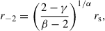 (A.5)
(A.5)
where r−2 is the radius at which the logarithmic DM slope is equal to −2.
The concentration cvir is defined as
 (A.6)
(A.6)
where rvir is the virial radius of the halo. We note that the halo concentration parameter cvir can be corrected to a DM-only halo, for example following the prescriptions of Katz et al. (2017) as
![Mathematical equation: $$ \begin{aligned} c_{\rm {vir, DMO}} = \frac{ c_{\rm {vir},-2} }{1+ e^{0.00001[3.4(X + 4.5)]}} . \end{aligned} $$](/articles/aa/full_html/2026/04/aa57396-25/aa57396-25-eq24.gif) (A.7)
(A.7)
(2) NFW: N-body DMO simulations predict cuspy DM halo profiles, which can be well described by the NFW profile (Navarro et al. 1997). This profile can be considered a special case of the generalised α − β − γ profile with α, β, γ = (1, 3, 1). The DM density profile is given by
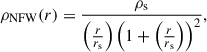 (A.8)
(A.8)
which goes as ρ ∝ r−1 at small radii and ρ ∝ r−3 at large radii.
(3) Dekel-Zhao: Freundlich et al. (2020b) introduce a halo profile with two shape parameters subject to baryonic effects, which is a special case of the generalised α − β − γ profile with α, β, γ = (0.5, 3.5, γ). This profile has a variable inner slope, γ, and concentration parameter cvir, and the profile parameters are correlated with the stellar-to-halo mass ratio, thereby being appropriate for describing both cusped and cored density profiles. The DM density profile is given by
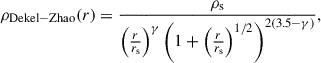 (A.9)
(A.9)
with  , while
  ,
,  and
and  , and two shape parameters γ, and the concentration parameter cvir. The variable inner slope, γ, defined in Freundlich et al. (2020b) as the absolute value of the logarithmic slope at 1% of the virial radius (denoted as s1), depends on the stellar mass- halo mass relation as
 (A.10)
with X = M★/Mvir. The inner slope corresponds to the NFW slope for log(M★/Mvir) < − 4, to flatter inner density profiles for log(M★/Mvir) between −3.5 and −2 and to steeper than NFW inner density profiles for log(M★/Mvir) > − 2.
(4) Burkert: Burkert (1995) introduced a halo profile characterised by a cored structure, i.e. with a finite density towards the centre, as opposed to the diverging density seen in the NFW profile. The density profile is given by
 (A.11)
(5) coreNFW: Read et al. (2016) studied the evolution of isolated dwarf galaxies using high-resolution hydrodynamic simulations, and showed that repeated bursts of SF can transform cusps into cores. A general fitting function for the evolved DM profile, based on the NFW profile, was introduced:
 (A.12)
where
 (A.13)
This function suppresses the central cusp below a core radius, rc, defined as rc = ηR1/2, with η = 1.75 and R1/2 being the half mass radius. The parameter n controls the shallowness of the core, where n = 0 corresponds to a cusp and n = 1 to a core. This parameter is tied to the SF time scale tSF, set to be ∼5.8 Gyr for z ∼ 1 SFGs. The resulting density profile for coreNFW is given by
 (A.14)
(6) Einasto: Using high-resolution N-body simulations, Navarro et al. (2004) demonstrated that the DM halos are better described by the Einasto profile (Einasto 1965), which has the following density profile:
 (A.15)
Here αϵ is a shape parameter describing the rate at which the logarithmic slope decreases towards the centre. When αϵ > 0, the profile has a finite density. For example, Dutton & Macció (2014) have shown that αϵ is dependent on the halo mass; however, we chose to leave this parameter free in our modelling and impose flat priors such that αϵ ∈ [0.1, 2].
(7) Baryons-only: We also tested baryon-only models, performing the RC decomposition by assuming maximal disks, i.e. without any contribution from a DM halo. We thereby set vDM(r)2 = 0 in Eq. 1.
Table A.1 presents the free parameters used in our models, which are detailed in Sect. 2.3.
Parameters used in the GALPAK3D modelling, as described in Sects. 2.1 and 2.2.
Appendix B: Impact of different HI parametrisations
To assess the impact of the HI surface density model used in our disk-halo decomposition (Sect. 2.2) on the recovered DM halo parameters, we compared in Fig. B.1 the inferred inner DM slope γ obtained with three different assumptions for the HI distribution. Our model (i) assumes a constant HI surface mass density (ΣHI∼ct.), yielding  , and results in a slope γsgas. We contrast this with results obtained using the models (ii) and (iii) assuming radially declining profiles from Martinsson et al. (2016, γMartinsson, left panel) and Wang et al. (2025, γWang, right panel), respectively. All decompositions assumed the DC14 profile for the DM halo.
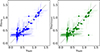 |
Fig. B.1. Comparison of the inner DM slope γ obtained using different HI surface density models in the disk-halo decomposition. Shown are the constant HI surface mass density vs the Martinsson et al. (2016) profile (left) and vs the Wang et al. (2025) profile (right). The error bars indicate 95% confidence intervals from the MCMC posterior. The dashed 1:1 line marks perfect agreement. |
We find good agreement within the uncertainties for 90% of the sample, indicating that our conclusions are robust against reasonable variations in the assumed HI profile. The uncertainties on γ incorporate the full posterior distribution from the MCMC sampling and therefore account for the propagated uncertainty in the gas contribution.
Appendix C: Example posterior distributions
Figures C.1, C.2, and C.3 show corner plots of the posterior distributions for the three representative galaxies shown throughout the main text– IDs 26, 6877, and 958 (from Fig. 6)– based on the DC14 fits. The diagonal panels display the marginalised one-dimensional distributions for each parameter, while the off-diagonal panels show two-dimensional scatter plots of all sample pairs. These examples illustrate the typical behaviour discussed in the main text: most parameters exhibit well-behaved, approximately Gaussian posteriors with minimal degeneracies, which are data-driven and not prior-dominated. We note that the concentration (cvir) shows some correlation with the virial velocity (vvir), as expected from cvir = Rvir/rs. Similar correlations are present for log(X) and vvir (or Mvir) and for log(X) and M★, noting that M★ is derived from log(X), rather than independently fitted.
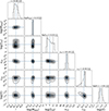 |
Fig. C.1. Corner plot for galaxy MXDF 26 showing the posterior distributions of the model parameters for the DC14 fits. The diagonal panels display the one-dimensional marginalised distributions for each parameter. The values of the best-fit parameters and associated errors (68% confidence intervals) are shown as the dashed blue and black lines, respectively. The off-diagonal panels show the two-dimensional joint distributions, highlighting correlations between parameters. Contours in the two-dimensional plots represent the 1σ, 2σ, and 3σ confidence regions. |
Appendix D: Mass maps
To create resolved stellar mass maps, we used the HST/ACS F435W, F606W, F775W, and F850LP bands from the Great Observatories Origins Deep Survey South (GOODS-S, Dickinson et al. 2003; Giavalisco et al. 2004) and we added the F814W from the Cosmic Assembly Near-IR Deep Extragalactic Legacy Survey (CANDELS, Grogin et al. 2011; Koekemoer et al. 2011). For JWST, we used the NIRCAM F090W, F115W, F150W, F200W, F277W, F335M, F356W, F410M, and F444W bands from the JWST Advanced Deep Extragalactic Survey DR3 (JADES, Bunker et al. 2024; Eisenstein et al. 2026, 2025; Rieke et al. 2023; D’Eugenio et al. 2025). We also complemented the observations with additional JWST/NIRCam medium bands from the JWST Extragalactic Medium-band Survey (JEMS, Williams et al. 2023a,b) as provided as part of JADES since its DR2. This includes the F182M, F210M, F430M, 460M, and 480M bands. We did not consider the HST/WFC3 F105W, F125W, F140W, and F160W bands from CANDELS since the images are only available at a coarser pixel scale of either 40mas or 60mas. In the end, we used five HST/ACS bands in the optical and 14 JWST/NIRCAM bands in the NIR (from roughly 400nm to 5μm) to reconstruct spatially resolved maps of the stellar mass of the galaxies.
For each galaxy, we extracted 200 × 200 pixels cutouts and variance maps in all aforementioned bands and converted them to the same flux unit. For JWST, variance maps were taken as the square of the error map that includes all sources of uncertainties, whereas, for HST, the variance maps were taken as the inverse of the weight maps (Casertano et al. 2000) and, by construction, do not include Poisson noise. Thus, we added in quadrature the contribution of Poisson noise to the HST variance maps following the prescription given in Sect. 8.1 of Mercier (2023). Then, we convolved each cutout to the spatial resolution of the F480M band14 using a matching kernel for the image and the square of the kernel for the variance map (see Sect. 8.1 and Appendix D of Mercier 2023). The HST PSFs were produced using the Photutils (Bradley et al. 2024) implementation of the ePSF empirical reconstruction method (Anderson & King 2000; Anderson 2016) using a maximum of 30 iterations and a sigma clipping of five. To reconstruct the best-fit ePSF model, we used a set of five nearby stars taken from the MXDF analysis that are located in the vicinity of the MHUDF. For JWST, we created PSF models for the JADES observations using WebbPSF (Perrin et al. 2012, 2014), following Rieke et al. (2023). We did not estimate PSF variations across the field of view since the MHUDF is a relatively small field. After producing all the PSF models, we created for each band the matching kernel to F480M using the PyPHER software (Boucaud et al. 2016) and convolved the images and the variance maps in this band using this kernel. The F480M PSF was also adopted in our MGE modelling (Sect. 5.2.1) to ensure consistency with the PSF-matched data and resulting mass maps.
We used the pixel-per-pixel SED fitting library pixSED to produce spatially resolved stellar mass maps from the PSF-matched HST and JWST images of the galaxies. An account of how the library works can be found in Sect. 8 of Mercier (2023). Effectively, it acts as a wrapper that takes as input the redshift along with multi-band images and variance maps of a galaxy and produces resolved maps of physical parameters (e.g. stellar mass or SFR) using already existing SED fitting codes as backend. In this analysis, we used the SED fitting code Cigale (Boquien et al. 2019). Each pixel was fitted separately assuming a Chabrier IMF (Chabrier 2003), Bruzual & Charlot (2003) single stellar populations, a delayed exponential SFH with a final burst or quench episode (Ciesla et al. 2018, 2021), and a Charlot & Fall (2000) attenuation law. Nebular emission was also included in the fit, using the default Cigale parameters. Specifically, we adopted an ionisation parameter of log(U) = − 2, assumed no Lyα photons escape, and used a default line width of 300 km/s. Furthermore, we added in quadrature a 10% uncertainty on the fluxes, which is standard practice in SED fitting, with this treatment accounting for both calibration and model uncertainties (e.g. Arango-Toro et al. 2025). To speed up the fitting process, we masked beforehand pixels that belong to nearby galaxies using the segmentation maps provided as part of JADES, and we kept the background pixels to estimate the uncertainties on the stellar mass at the pixel level when fitting pure background fluctuations.
We show a typical example for galaxy 939 at z ≈ 1.3 in Fig. D.1. When integrating the stellar mass map within the area defined by the JADES segmentation map, we find a total stellar mass equal to log(M★/M⊙) = 10.01, similar to what was obtained in Bacon et al. (2023) with Magphys, namely log(M★/M⊙) = 10.14. It is worth mentioning that we observe good agreement between the M★ obtained from the different SED fitting routines outlined in Sect. 4.3 and in this section.
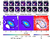 |
Fig. D.1. Example of a stellar mass map and its associated bulge-disk decomposition for galaxy 939, which has a B/T = 0.22. The top two rows show cutouts of the galaxy in the different HST and JWST bands that were used for the pixel-per-pixel SED fitting (arbitrary unit). The bottom row shows the reconstructed stellar mass map (left), the best-fit bulge-disk decomposition obtained on the mass map (middle), and the residuals (right). The black line denotes the limits of the galaxy as determined by the segmentation map provided as part of the JADES survey. |
Appendix E: Model residuals and Bayes factor
Here we explore the connection between the residual maps and the Bayes factor, which is used to select the best-fitting model for our sample in Sect. 5.1. Figure E.1 shows the residual maps (generated from the residual cube as in Fig. 6) for each of the six DM profiles–DC14, NFW, Burkert, Dekel-Zhao, Einasto, coreNFW– and the baryon only model for the same three galaxies from Fig. 6 and one more representative galaxy from our sample. On the maps, we report the Bayesian evidence (black text) and the Bayes factor (colour-coded as in Fig. 8) between DC14 and the competing models. These examples illustrate the link between the Bayes factor and the structure of the residuals: whenever the Bayes factor indicates strong evidence in favour of one model, i.e. Δlog(𝒵)≪ − 6, the corresponding residual map of the best-fit model consistently displays lower residuals than those of the competing models. For instance, for galaxy MOSAIC 888, we infer a Bayes factor of Δlog(𝒵) = − 1141 between the DC14 and NFW profiles, and Δlog(𝒵) = − 1523 between the DC14 and the baryon-only models, indicating a very strong positive evidence for DC14. The figure shows that the baryon-only and NFW models are strongly disfavoured, as reflected in their pronounced residuals. However, when we infer a Bayes factor with a small value between two competing models (−6 < Δlog(𝒵) < 6 - inconclusive or mild positive or mild negative evidence - see middle two panels of Fig. E.1), the residual maps look fairly similar.
 |
Fig. E.1. Residual maps derived by computing the standard deviation along the wavelength axis of the residual cube, shown for all six halo models and the baryon-only model for the same galaxies shown in Fig. 6 and one more representative galaxy from our sample, for which we find mainly strong positive evidence for the DC14 model over the alternatives (except for Einasto and coreNFW). The titles of each panel show the log(𝒵) inferred from our MCMC fitting routine for the respective model. The Bayes Factor computed for each model against DC14 is shown in each panel, colour-coded as in Fig. 8. |
Appendix F: Stellar mass halo mass relation for all halo models
Figure F.1 displays the M★ − Mvir relation, where M★ is inferred from SED-fitting, and Mvir from the disk-halo decomposition using all six different halo models. As discussed in the main text, this Fig. demonstrates that the DC14 model yields the tightest M★ − Mvir, followed by Dekel-Zhao, in qualitative agreement with the predictions from Behroozi et al. (2019) and Girelli et al. (2020), albeit with larger scatter. The M★ − Mvir relations obtained using NFW, Burkert, Einasto and coreNFW display a much larger scatter with respect to the expected relation. Additionally, when using the other models, some galaxies exhibit Mvir < M★ (for instance, as seen in the second panel from the top, where we have used the NFW profile). Upon investigating these outliers, we discovered that they are galaxies that exhibit a strong preference for cored DM distributions. Consequently, the NFW fits produce unphysical results for these cases.
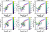 |
Fig. F.1. Stellar mass – halo mass relation for the MHUDF sample using the six halo models. The solid red curve shows the relation from Behroozi et al. (2019) for the mean redshift of our sample, z = 0.85, while the red shaded region shows the scatter of the relation. The solid blue curve shows the relation inferred by Girelli et al. (2020) for 0.8< z< 1.1, whereas the blue shaded region shows the scatter of the relation. The circles depict the regular galaxies, whereas the stars represent the perturbed galaxies from our sample. The data points are colour-coded according to their z. To improve the readability, the error bars show the 65% CI (∼1σ symmetric errors). |
Appendix G: Concentration halo mass relation for all halo models
Figure G.1 displays the cvir − Mvir relation inferred from all six different halo models. This figure demonstrates that the DC14 model yields the tightest cvir − Mvir, while the parameters inferred from the other models display a much larger scatter with respect to the simulated relation (Dutton & Macció 2014), yielding by far higher concentration values than expected.
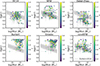 |
Fig. G.1. Concentration – halo mass relation for our sample using all six halo models. The solid grey line shows the cvir − Mvir relation from Dutton & Macció (2014) for the mean z of our sample, z = 0.85, while the shaded grey region shows the scatter of the relation. The circles depict the regular galaxies, whereas the stars represent the perturbed galaxies from our sample. The data points are colour-coded according to their z. To improve the readability, the error bars show the 65% CI (∼1σ symmetric errors). |
Appendix H: Best-fit parameters
In Table H.1 we present the best-fit parameters for the same three galaxies (ID 26, 6877, 958) shown in Fig. 6 using all the differen DM models, namely (1) the DC14 profile (Di Cintio et al. 2014); (2) NFW (Navarro et al. 1997); (3) Burkert (Burkert 1995); (4) Dekel-Zhao (Freundlich et al. 2020b); (5) Einasto (Navarro et al. 2004); and (6) coreNFW (Read et al. 2016). We provide the MUSE IDs, indicate the respective DM model and list best-fit parameters such as the virial velocity, Vvir, in [km/s], the virial mass in log-scale, log Mvir [M⊙], the concentration, cvir, and the scale radius, rs, in [kpc]. For every parameter, we also report its 95% confidence interval, computed from the 2.5 and 97.5 percentile bounds of the posterior distribution. A full catalogue can be made available upon request or can be found on the DARK webpage.
Best-fit parameters inferred from the disk–halo decomposition using all six DM models.
All Tables
Parameters used in the GALPAK3D modelling, as described in Sects. 2.1 and 2.2.
Best-fit parameters inferred from the disk–halo decomposition using all six DM models.
All Figures
|
Fig. 1. Results from the 3D disk-halo decomposition applied to the mock MUSE cube of the simulated galaxy ID3. Panel (a): Mock MUSE white-light image with flux intensity contours overlaid. Panel (b): Position velocity diagram. The observed velocity profiles as measured with GALPAK3D and MPDAF (Bacon et al. 2016) are overlaid in red and green, respectively. The dotted black line shows the region beyond which the S/N of the emission line falls below unity, whereas the white contours show the flux intensity. Panels (c) and (d): Observed velocity field obtained using a traditional 2D line fitting code and the modelled velocity field obtained from 3D disk-halo decomposition with GALPAK3D. Panel (e): Contribution of the different components (stars-orange, gas-blue, DM-green curve) to the RC (dot-dashed curve; corrected for pressure support). Panel (f): Measured DM density profile (in green) compared to the true DM density profile (in red). The light shaded regions in these two panels show the 95% confidence interval. Panel (g): Posterior distributions (in blue) for a subset of the parameters we fit for: log(X) = log(M★/Mhalo), the virial velocity, the concentration, and the disk inclination. Panel (h): Posterior distributions for parameters derived from the fitted ones, including the DM density profile shape parameters α, β, and γ (computed using Eqs. (A.2), (A.3), and (A.4), respectively), as well as the stellar mass log(M★/M⊙). The recovered values are shown as the dark blue lines, while the values used as inputs for the simulation are shown as the red lines. |
| In the text | |
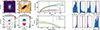 |
Fig. 2. Same as Fig. 1, but for the mock MUSE cube of the simulated galaxy ID982. |
| In the text | |
|
Fig. 3. Left: Effective S/N for the brightest emission line using Eq. (3), as a function of the S/N of the total line flux from the integrated spectrum. Right: Ratio of the stellar half-light radius to the PSF radius as a function of the S/N in the brightest spaxel. The grey shaded area in the panels marks the exclusion region, i.e. all galaxies with S/Neff < 10 and Re/RPSF < 0.5 are removed from the sample. The data points are colour-coded according to their half-light radii. The circles, stars, diamonds, and squares represent the [OII], Hα, Hβ, and [OIII] emitters, respectively. |
| In the text | |
|
Fig. 4. Left: Histogram showing the redshift distribution of the MHUDF SFGs. Middle: Histogram showing the stellar mass distribution of sample (Bacon et al. 2023). Right: Histogram showing the distribution of the Sérsic indices (van der Wel et al. 2012). |
| In the text | |
|
Fig. 5. Stellar mass – SFR relation for the MHUDF sample. The data points are colour-coded according to their effective S/N (Eq. (3)). The black line shows the star-forming main sequence at z = 0.85 (the mean redshift of our sample), as derived by Boogaard et al. (2018), whereas the grey shaded region shows the 0.44 dex scatter around the relation. The grey cross in the lower right corner indicates the median 1σ statistical uncertainties in M★ and SFR from Magphys. |
| In the text | |
|
Fig. 6. Example of morpho-kinematic maps for three galaxies, ID 26, 6877, and 958, covering the range of S/N ∼28 − 116. For each galaxy, the 11 panels show (a) the HST F160W image; (b) the emission-line flux map, with the S/N contours overlaid; (c+d) the observed velocity maps in [km/s] with the CAMEL (Epinat et al. 2012) and with GALPAK3D (URC), with the grey line showing the major-axis; (e) the observed velocity profile v⊥(r)sin(i)obs extracted along the major-axis; (f) the position-velocity diagram extracted along the major-axis; (g) the intrinsic velocity profile v⊥(r), i.e. corrected for inclination and instrumental effects; (h+i) the observed velocity dispersion maps in [km/s]; (j) the intrinsic velocity dispersion profile in [km/s]; and (k) the residuals map derived by computing the standard deviation along the wavelength axis of the normalised residual cube (see Bouché et al. 2022). In panels e, f, and g, the vertical dashed black line represents the radius at which the S/N ≃1, whereas the vertical dotted (light) green lines represent (3Re) 2Re. |
| In the text | |
|
Fig. 7. Left: RCs (using the URC model, Sect. 2.1) of our sample of intermediate-z SFGs, colour-coded by stellar mass. The dotted black line shows the physical extent of 1 MUSE spaxel at z ∼ 1, namely 1.65 [kpc]. Right: Inner RC slopes, S (corrected for inclination), as a function of the stellar mass surface density. The data points are colour-coded according to their z. The error bars on the y-axis show the 95% confidence intervals from our 3D kinematic modelling, while the x-axis shows the 1σ uncertainties in ΣM★. |
| In the text | |
|
Fig. 8. Histograms showing the Bayes factor for all the pairs of halo models used in this study. The red columns show the number of galaxies that display a very strong positive evidence towards the first model, i.e. which have −103 < Δ log(𝒵) < −20. The two lighter red columns depict the number of galaxies that show strong positive evidence and positive evidence for the first model, i.e. which have −20 < Δ log(𝒵) < −6 and −6 < Δ log(𝒵) < −2, respectively. The blue columns show the number of galaxies that show very strong positive evidence for the second model, i.e. 20 < Δ log(𝒵) < 103, while the lighter blue columns display the number of systems that show strong positive evidence and positive evidence for the second model, namely 6 < Δ log(𝒵) < 20 and 2 < Δ log(𝒵) < 6, respectively. The grey columns display the number of galaxies for which both models perform similarly, having −2 < Δ log(𝒵) < 2. In each panel, model 1 refers to the first model listed in the title, while model 2 refers to the second model. |
| In the text | |
|
Fig. 9. Examples of the 3D disk-halo decomposition for the three galaxies show in Fig. 6 using a DC14 DM profile (Eq. (A.1)). The solid black line represents the rotational velocity v⊥(r). The thick dashed black line represents the circular velocity vc(r), i.e. v⊥(r) corrected for pressure support (Sect. 2.2). The green curve represents the RC of the DM component. The solid orange and blue curves represent the disk and H I components, respectively. The light shaded regions show the 95% confidence intervals. The dotted brown lines represent the stellar component obtained using the MGE modelling of the stellar mass maps (see Sect. 5.2.1). All velocities are intrinsic, i.e. corrected for inclination and instrumental effects, including seeing (PSF). The black dotted line shows the physical extent of a MUSE spaxel, the dot-dashed red line shows 2 × Re, while the dashed grey line shows the region beyond which S/N < 1. |
| In the text | |
|
Fig. 10. Comparison of DM velocity profiles for the three galaxies shown in Fig. 9. The green curves show the profiles modelled with GALPAK3D assuming a DC14 halo, while the purple curves are obtained by subtracting the baryonic contributions obtained with vcdisk from the MUSE-derived vc(r). The green shaded regions indicate the 95% confidence intervals from the 3D disk–halo decomposition fits. |
| In the text | |
|
Fig. 11. Left: Comparison between the stellar masses inferred from our disk-halo decomposition using the DC14 halo model and the stellar masses inferred from photometric observations. The dashed black line shows the 1:1 relation, and the grey shaded region shows the 0.5 dex dispersion around the relation. The data points are colour-coded according to their S/Neff. Right: DM inner slope, γ, as inferred from the DC14 halo model as a function of the stellar masses derived from SED fitting. The data points are colour-coded according to their virial masses. The coloured curves depict the parametrisation of Di Cintio et al. (2014) for γ (Eq. (A.4)), for four different virial masses, as indicated in the legend. In both panels, the circles show the regular MHUDF galaxies, while the stars depict the perturbed galaxies from our sample. The error bars represent the 95% confidence intervals. |
| In the text | |
|
Fig. 12. DM fractions within Re as a function of the stellar mass surface density. The black diamonds show the DM fractions inferred by Puglisi et al. (2023) for z ∼ 1.5 SFGs, the black squares depict the z = 1 − 2 sample of Genzel et al. (2020), while the black triangles show the RC100 sample from Nestor Shachar et al. (2023). Our sample is colour-coded according to its redshifts. The circles depict the regular galaxies, while the stars represent the perturbed systems from our sample. The error bars represent the 95% confidence intervals. The red dotted line shows the toy model derived from the Tully–Fisher relation (see Bouché et al. 2022, Sect. 5.1). |
| In the text | |
|
Fig. 13. Example of DM density profiles for the same three galaxies shown in Fig. 9. The y-axis shows the DM density, ρDM(r), in units of M⊙/kpc3, and the x-axis the r/Re. The red curve shows the DM density profile obtained using the DC14 halo model, whereas the red-shaded region represents the 95% confidence interval. The inferred DM inner slopes, γ, are indicated in the upper left corner of each panel. The vertical dashed black lines represent the 0.2″ spaxel scale, indicating the lower limit of our constraints. |
| In the text | |
|
Fig. 14. Left: Concentration–halo mass relation for the MHUDF sample. The solid coloured lines show the cvir − Mvir relation from Dutton & Macció (2014) for 0.3 < z < 1.5, while the shaded regions show the 0.11 dex scatter around the relations. The data points are colour-coded according to their redshifts. Right: rs, DMO = rvir/cvir in [kpc] as a function of the halo masses. The dotted black line displays the observed scaling relation for z = 0 low surface brightness systems inferred by Di Paolo et al. (2019), while the solid black line shows the predictions from Dutton & Macció (2014). The data points are colour-coded according to their effective S/N. In both panels, the circles show the regular MHUDF galaxies, while the stars depict the perturbed galaxies. The error bars represent the 95% confidence intervals. |
| In the text | |
|
Fig. 15. Panel (a): Halo scale radius–DM density relation for the MHUDF sample. The dashed black line shows the relation inferred by Di Paolo et al. (2019) for z = 0 low surface brightness galaxies, while the dashed red line shows the relation derived by Kormendy & Freeman (2016) for z = 0 SFGs. The purple line shows a power-law fit to our mass complete sample, with |
| In the text | |
|
Fig. 16. Panel (a): Stellar masses of the entire MHUDF sample (with log(M★/M⊙) > 8.5) as a function of the offset from the SFMS (ΔMS) from Boogaard et al. (2018). The data points are colour-coded according to the DM inner slope, γ. The error bars show the 1σ statistical uncertainties in M★ and SFR from Magphys. Panel (b): DM density at 150 pc as a function of log(M★/Mvir). The data points are colour-coded according to their sSFRs. The error bars represent the 95% confidence intervals from our disk-halo decomposition. In both panels, the circles show the regular MHUDF galaxies, while the stars depict the perturbed systems from our sample. Panel (c): γ as a function of the stellar masses for the mass-matched MHUDF sample (red circles) and the TNG galaxies (black open squares, from Pillepich et al. 2019). The large indigo data points show the mean values for γ of the MHUDF sample in 6 mass bins, while the grey diamonds show the mean values for the mass-matched SPARC sample at z = 0 (using the DC14 fits without ΛCDM priors from Li et al. 2020). The green curve shows the predictions from Tollet et al. (2016) at z = 0, whereas the green shaded region shows the 0.18 dex scatter around the relation. The histogram shows the distribution of the γ values for the mass-matched MHUDF (in red), SPARC (in grey), TNG (in black), and NIHAO (in green) samples. |
| In the text | |
|
Fig. B.1. Comparison of the inner DM slope γ obtained using different HI surface density models in the disk-halo decomposition. Shown are the constant HI surface mass density vs the Martinsson et al. (2016) profile (left) and vs the Wang et al. (2025) profile (right). The error bars indicate 95% confidence intervals from the MCMC posterior. The dashed 1:1 line marks perfect agreement. |
| In the text | |
|
Fig. C.1. Corner plot for galaxy MXDF 26 showing the posterior distributions of the model parameters for the DC14 fits. The diagonal panels display the one-dimensional marginalised distributions for each parameter. The values of the best-fit parameters and associated errors (68% confidence intervals) are shown as the dashed blue and black lines, respectively. The off-diagonal panels show the two-dimensional joint distributions, highlighting correlations between parameters. Contours in the two-dimensional plots represent the 1σ, 2σ, and 3σ confidence regions. |
| In the text | |
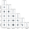 |
Fig. C.2. Same as C.1, but for galaxy MOSAIC 6877. |
| In the text | |
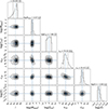 |
Fig. C.3. Same as C.1, but for galaxy MOSAIC 958. |
| In the text | |
|
Fig. D.1. Example of a stellar mass map and its associated bulge-disk decomposition for galaxy 939, which has a B/T = 0.22. The top two rows show cutouts of the galaxy in the different HST and JWST bands that were used for the pixel-per-pixel SED fitting (arbitrary unit). The bottom row shows the reconstructed stellar mass map (left), the best-fit bulge-disk decomposition obtained on the mass map (middle), and the residuals (right). The black line denotes the limits of the galaxy as determined by the segmentation map provided as part of the JADES survey. |
| In the text | |
|
Fig. E.1. Residual maps derived by computing the standard deviation along the wavelength axis of the residual cube, shown for all six halo models and the baryon-only model for the same galaxies shown in Fig. 6 and one more representative galaxy from our sample, for which we find mainly strong positive evidence for the DC14 model over the alternatives (except for Einasto and coreNFW). The titles of each panel show the log(𝒵) inferred from our MCMC fitting routine for the respective model. The Bayes Factor computed for each model against DC14 is shown in each panel, colour-coded as in Fig. 8. |
| In the text | |
|
Fig. F.1. Stellar mass – halo mass relation for the MHUDF sample using the six halo models. The solid red curve shows the relation from Behroozi et al. (2019) for the mean redshift of our sample, z = 0.85, while the red shaded region shows the scatter of the relation. The solid blue curve shows the relation inferred by Girelli et al. (2020) for 0.8< z< 1.1, whereas the blue shaded region shows the scatter of the relation. The circles depict the regular galaxies, whereas the stars represent the perturbed galaxies from our sample. The data points are colour-coded according to their z. To improve the readability, the error bars show the 65% CI (∼1σ symmetric errors). |
| In the text | |
|
Fig. G.1. Concentration – halo mass relation for our sample using all six halo models. The solid grey line shows the cvir − Mvir relation from Dutton & Macció (2014) for the mean z of our sample, z = 0.85, while the shaded grey region shows the scatter of the relation. The circles depict the regular galaxies, whereas the stars represent the perturbed galaxies from our sample. The data points are colour-coded according to their z. To improve the readability, the error bars show the 65% CI (∼1σ symmetric errors). |
| In the text | |
Current usage metrics show cumulative count of Article Views (full-text article views including HTML views, PDF and ePub downloads, according to the available data) and Abstracts Views on Vision4Press platform.
Data correspond to usage on the plateform after 2015. The current usage metrics is available 48-96 hours after online publication and is updated daily on week days.
Initial download of the metrics may take a while.