| Issue |
A&A
Volume 706, February 2026
|
|
|---|---|---|
| Article Number | A57 | |
| Number of page(s) | 40 | |
| Section | Planets, planetary systems, and small bodies | |
| DOI | https://doi.org/10.1051/0004-6361/202554644 | |
| Published online | 04 February 2026 | |
ExoplaNeT accRetion mOnitoring sPectroscopic surveY (ENTROPY)
II. Time series of Balmer line profiles of Delorme 1(AB)b★
1
Université Grenoble Alpes, CNRS,
IPAG,
38000
Grenoble,
France
2
Institutionen för astronomi, Stockholms universitet,
AlbaNova universitetscentrum,
106 91
Stockholm,
Sweden
3
Institute for Advanced Study, Tsinghua University,
Beijing
100084,
PR China
4
Department of Astronomy, Tsinghua University,
Beijing
100084,
PR China
5
Department of Earth and Planetary Science, The University of Tokyo,
7-3-1 Hongo, Bunkyo-ku,
Tokyo
113-0033,
Japan
6
Department of Physics, Faculty of Science, Chulalongkorn University,
254 Phayathai Rd.,
Patumwan, Bangkok
10330,
Thailand
7
Institute for Astrophysical Research and Department of Astronomy, Boston University,
725 Commonwealth Ave.,
Boston,
MA
02215,
USA
8
Division of Space Research & Planetary Sciences, Physics Institute, University of Bern,
Sidlerstr. 5,
3012
Bern,
Switzerland
9
Max-Planck-Institut für Astronomie,
Königstuhl 17,
69117
Heidelberg,
Germany
10
Fakultåt für Physik, Universitåt Duisburg-Essen,
Lotharstraße 1,
47057
Duisburg,
Germany
11
European Southern Observatory,
Karl-Schwarzschild-Straße 2,
85748
Garching bei München,
Germany
12
INAF/Osservatorio Astronomico di Padova,
Vicolo dell’Osservatorio 5,
35122
Padova,
Italy
13
Department of Physics, ETH Zürich,
Wolfgang-Pauli-Str. 27,
8093
Zürich,
Switzerland
14
SUPA, School of Science and Engineering, University of Dundee,
Nethergate,
DD1 4HN, Dundee,
UK
15
Millennium Nucleus on Young Exoplanets and their Moons (YEMS),
Santiago,
Chile
16
Instituto de Estudios Astrofísicos, Facultad de Ingeniería y Ciencias, Universidad Diego Portales,
Av. Ejército 441,
Santiago,
Chile
★★ Corresponding authors: This email address is being protected from spambots. You need JavaScript enabled to view it.
; This email address is being protected from spambots. You need JavaScript enabled to view it.
Received:
19
March
2025
Accepted:
3
November
2025
Abstract
Context. Accretion processes in the planetary-mass regime are still poorly constrained, yet they strongly impact the formation and evolution of planets and the composition of circumplanetary disks.
Aims. We investigate the resolved Balmer hydrogen emission-line profiles and their variability timescales in the ∼13 MJup, 30−45 Myr-old companion Delorme 1 (AB)b to derive constraints on the accretion mechanism at play.
Methods. With VLT/UVES, we collected 31 new epochs of high-resolution optical (330–680 nm) spectra of the companion at R = 50 000, probing variability on timescales of hours to years. We study the companion’s H i emission line shape and flux variability and compare them to two proposed line origins: magnetospheric accretion funnel and localized accretion shock.
Results. We detect H i Balmer lines from Hα up to H10 (6564–3799 Å), as well as the UV continuum excess – signs of ongoing accretion. All lines and UV excess are variable. The H i lines can be decomposed into two static components that vary only by their flux. The broader component in velocity correlates strongly with the UV excess, and its profile is qualitatively reproduced by magnetospheric accretion funnel models but clearly not by shock models. With strong relative variability, this broad component almost entirely explains the variability in the shape of the line profiles. The second, narrower component correlates less with the UV excess and is best reproduced by shock-emission models. Its strong absolute variability makes it responsible for most of the line flux variability. Overall, the lines have low relative flux variability on hourly timescales, but up to ∼100% on weekly timescales and beyond, a behavior similar to T Tauri stars.
Conclusions. The properties of the broad component of the H i lines strongly support magnetospheric accretion. The narrow component could be due to an accretion shock as well as chromospheric activity. Higher-cadence observations could search for rotational modulations to constrain the object’s rotational period and the exact geometry of the accretion flow.
Key words: accretion, accretion disks / planets and satellites: formation / planets and satellites: individual: Delorme 1 (AB)b
Based on observations collected at the European Organization for Astronomical Research in the Southern Hemisphere under ESO programs 108.21ZE.001 and 110.23VU.001.
© The Authors 2026
 Open Access article, published by EDP Sciences, under the terms of the Creative Commons Attribution License (https://creativecommons.org/licenses/by/4.0), which permits unrestricted use, distribution, and reproduction in any medium, provided the original work is properly cited.
This article is published in open access under the Subscribe to Open model. This email address is being protected from spambots. You need JavaScript enabled to view it. to support open access publication.
1 Introduction
A few tens of planetary-mass objects (PMOs) and planetarymass companions (PMCs) have been found to display emission lines at optical and near-infrared (NIR) wavelengths (e.g., Hα at 6563 Å and Paβ at 1.282 μm; see Betti et al. 2023 for a recent compilation) indicative of active accretion. These objects are members of star-forming regions or nearby-young associations, with masses down to 5 MJup (Lodieu et al. 2018; Luhman et al. 2023), and are found as free-floating objects (e.g., Muzerolle et al. 2005; Joergens et al. 2013; Lodieu et al. 2018), companions to single stars, or binaries of various masses (Petrus et al. 2020; Zhang et al. 2021; Chinchilla et al. 2021). Some are embedded in circumstellar disks (the emblematic and so far unique case of PDS 70 b and c; Haffert et al. 2019), while others are found outside these primordial disks (e.g., Seifahrt et al. 2007; Santamaría-Miranda et al. 2018; Santamaría-Miranda et al. 2019).
Recent efforts to derive accretion rates suggest that the Ṁ−M* correlation derived in the stellar regime flattens out in the planetary-mass range (Ayliffe & Bate 2009; Betti et al. 2023), therefore suggesting different mechanisms driving accretion in that mass interval. Betti et al. (2023) also found a steepening of the Ṁ−M relation with age in the brown-dwarf mass regime, down to the deuterium-burning limit (approximately 13.6 MJup; Spiegel et al. 2011), which increases with age above 3 Myr. Almendros-Abad et al. (2024) provided similar hints at younger ages (<3 Myr).
A few PMOs in nearby young kinematic associations have recently been found to display bright emission lines linked to accretion (2MASS J02265658-5327032, Delorme 1 (AB)b, 2MASS J0249-0557 c; Boucher et al. 2016; Eriksson et al. 2020; Chinchilla et al. 2021). Their much later estimated ages (20–45 Myr) and the firm detection of disk excess emission – indicative of circumplanetary disk (CPD) – for one of them (2MASS J02265658-5327032) suggest that accretion can be sustained longer than on stars in the planetary-mass range.
Emission line properties (fluxes, line profiles, and ratios) can be compared to predictions from nascent accretion models in the planetary mass range. Simulations of planets embedded in circumstellar disks suggest polar inflow from the circumstellar disk onto the CPD or directly at the planet’s poles (Szulágyi et al. 2014), creating line-emitting regions at localized accretion shocks. Shock models have since been developed to predict the flux of the Balmer and Paschen line series (Aoyama et al. 2018). Their predicted Hα/Hβ ratios do not match the observational constraints for PDS 70 b (Aoyama & Ikoma 2019; Hashimoto et al. 2020). Hashimoto et al. (2020) proposed that extinction along the line of sight caused by circumstellar or circumplanetary material may be the key to matching the observations. The geometry of the material and gas dynamics around accreting companions is likely to be complex (Krapp et al. 2024) and may depend on circumstellar disk properties (Lega et al. 2024). Its effects on the line properties have begun to be investigated theoretically (Szulágyi & Ercolano 2020; Marleau et al. 2022) and have been proposed as a possible explanation for the low detection yield of deep-imaging campaigns seeking hydrogen line emissions from protoplanets nested within circumstellar disks (Cugno et al. 2019; Uyama et al. 2020; Zurlo et al. 2020; Huélamo et al. 2022; Follette et al. 2023; Chaushev et al. 2024).
Instead of protoplanetary-disk-to-planet mass transfer, planets may also accrete directly from their surrounding CPD, through either boundary-layer (Szulágyi et al. 2014, 2016; Owen & Menou 2016; Takasao et al. 2021) or magnetospheric accretion. Magnetospheric accretion models of T-Tauri stars have very recently been adapted to predict the line emissions of PMOs (Thanathibodee et al. 2019a).
Emission-line variability is ubiquitous in the stellar mass range and can inform us on the accretion mechanisms at play (for a review, see Fischer et al. 2023). It is presently poorly characterized for PMCs, despite its importance for optimizing detection campaigns targeting protoplanet line emissions. Wolff et al. (2017) found the Paβ line of DH Tau b (a ∼1 Myr old, ∼15 MJup companion; Itoh et al. 2005) to vanish within five weeks, although the observations were based on only four epochs. Zhou et al. (2021) set an upper limit of 30% for the variability of the Hα line of PDS 70 b over timescales of days to months, based on eight epochs. While the line of PDS 70 c was not detected in the 2020 data, it was detected later in 2024, reaching approximately twice the 2020 upper limit (Zhou et al. 2025). Wu et al. (2023) conducted a six-night monitoring campaign of FU Tau B (19 MJup) to search for rotational modulations of Hα, as suggested by magnetospheric accretion models, but their conclusions were limited by the sensitivity of the data. Additionally, Demars et al. (2023) collected J-band spectra (1.1−1.35 μm) of the 14 MJup and 10−30 MJup companions GSC 06214-00210 b and GQ Lup b, probing the variability of the Paβ line over timescales ranging from minutes to a decade. They find variability on all these timescales, but with higher amplitude on timescales greater than typical rotation periods (a few hours to several days for companions), a behavior commonly observed in T Tauri stars Costigan et al. (2014); Venuti et al. (2021); Zsidi et al. (2022).
Line profiles can also inform us on the gas kinematics properties of the accreting material near the shock front, the line-of-sight extinction, and on the accretion mechanisms (Marleau et al. 2022). The few single-epoch spectra at high spectral resolution (R > 20 000) gathered on bright 1−10 Myr and 10−20 MJup free-floating objects reveal significant diversity in line shapes (Muzerolle et al. 2005; Mohanty et al. 2005), suggesting a complex picture.
The characterization of emission line profiles in PMCs is just beginning. Santamaría-Miranda et al. (2018); Santamaría-Miranda et al. (2019) obtained medium-resolution (Rλ from 3890 to 5400) spectra of the line emission produced by the PMC SR 12 c. The Hα line profile exhibited a possibly asymmetric peak structure, which they attributed to magnetospheric accretion. Demars et al. (2023) modeled Paβ emission line profiles obtained at Rλ=1800−2360 of GSC 06214-00210 b and GQ Lup b with both 1D shock and magnetospheric accretion models and found that the blueshifted profiles of GQ Lup b could only be reproduced by magnetospheric accretion models, while those of GSC 06214-00210 b can be reproduced by both sets of models. Finally, Ringqvist et al. (2023) presented a near-UV spectrum at R ∼ 50 000 of the companion Delorme 1 (AB)b showing complex profiles that can be modeled using multiple Gaussian components. Their comparison to shock models implies a small line-emitting area of ∼1% relative to the planetary surface, consistent with magnetospheric accretion. This motivates a more in-depth characterization of these objects to confirm whether this mechanism is truly operating and universal in the planetary-mass regime.
We present VLT/UVES (Very Large Telescope / Ultraviolet and Visual Echelle Spectrograph) observations obtained as part of the ExoplaNeT accRetion mOnitoring sPectroscopic surveY (ENTROPY) survey, which aims to characterize accretion processes of PMOs through the monitoring of their emission lines at high spectral resolution. The first study presented two epochs of observations of the 7–21 MJup free-floating object 2MASS J11151597+1937266, showing Hα line profiles compatible with magnetospheric accretion and variability between epochs (Viswanath et al. 2024). In this study we focus on followup observations of Delorme 1 (AB)b using an identical technical setup as in Ringqvist et al. (2023) to investigate variability in line profiles, fluxes, and ratios in an attempt to constrain the accretion mechanism operating in this object.
This paper is organized as follows: We describe our target of interest in Sect. 2. We detail in Sect. 3 the observations and data reduction procedures. We present in Sect. 4 the main spectral features of Delorme 1 (AB)b, its line variability, and our decomposition. We model the lines and their subcomponents with accretion models in Sect. 5. We discuss the results in Sect. 6 and summarize our findings in Sect. 7.
2 Target description
Delorme 1 (AB)b (also known as 2MASS J01033563-5515561 (AB)b) is a wide-separation ∼13 MJup companion (∼1.77′′, i.e., 84 AU; Delorme et al. 2013), orbiting a tight pair (∼0.25′′, i.e., 12 AU) of M5–M6 (Kraus et al. 2014; Eriksson et al. 2020) stars (0.19 M⊙ and 0.17 M⊙) displaying emission lines as well. Delorme 1 (AB)b has a reported ∼ L0 spectral type (Eriksson et al. 2020). It is the nearest of all presently known accreting PMCs, located at 47.2 ± 3.1 pc (Riedel et al. 2014). The binary stars are proposed members of the Tucana-Horologium or Carina associations (Riedel et al. 2014), with estimated ages of ∼30−45 Myr old (Gagné & Faherty 2018; Galli et al. 2023). While relatively young, Delorme 1 (AB)b is much older than commonly studied young accreting companions.
Eriksson et al. (2020) first reported strong Hα, Hβ, helium, and Ca II emission lines in the medium-resolution (R ≈ 1740–3750) VLT/MUSE optical (480–930 nm) spectrum of Delorme 1 (AB)b. Using stellar relations (Alencar et al. 2012; Alcalá et al. 2017), they derived accretion rates of log(Ṁ/MJup/yr) ∼−9.4 to −9.8. Paβ, Paγ, and Brγ lines were then identified on that target (Betti et al. 2022a,b), yielding accretion rates of log Ṁ ∼−8.2 to −8.8 MJup/yr using the same scalings, and log Ṁ ∼−7.30 ± 0.30 MJup/yr using Ṁ−Lline relationships from Aoyama et al. (2018). The higher end of the Balmer series (e.g., Hγ, Hδ, and Hϵ) were then detected in Ringqvist et al. (2023) from which they derived an accretion rate of log Ṁ ∼−7.70 MJup/yr using planetary scaling, compatible with the value derived by Betti et al. (2022b) from NIR lines. The line profiles constrain the dynamical mass of the companion to 13 ± 5 MJup. Betti et al. (2022a,b) suggests the presence of a longlived “Peter Pan” disk, which may explain why the planet is still actively accreting. Both dust and gas signatures have now been detected around the companion by JWST (Mâlin et al. 2025) and confirm the existence of a mass reservoir.
Smoothed-particle hydrodynamic (SPH) simulations of the gas in the system were conducted to understand the formation mechanism of Delorme 1 (AB)b (Teasdale & Stamatellos 2024), but they could not account for both the accretion rate onto the companion and its location in the system. Delorme 1 (AB)b is a unique test bed for understanding the formation mechanisms and accretion in the planetary-mass regime. With its bright lines and a reasonable angular separation, Delorme 1 (AB)b allows for collecting spectra with seeing-limited, slit-based spectrographs, such as UVES.
3 Observations and data reduction
Delorme 1 (AB)b was observed with the UVES instrument (Dekker et al. 2000) at VLT/UT2, from October 13, 2022, to January 2, 2023 (program 0110.C-0203(A)): approximately one year after the observations presented in Ringqvist et al. (2023) (program 0108.C-0655(A)). The observations probed timescales of ∼20 minutes (time between successive exposures), days, months, and a year. The light was split by a dichroic (DIC#1, 390+580 nm) and sent into two arms (RED and BLUE) containing 0.8′′ wide slits and echelle spectrographs, which yielded spectra at resolving powers Rλ ≈ 50 000. The RED arm has a mosaic of two chips with a physical gap of 96 mm. The final spectra span 3300–4520 Å in the BLUE arm and 4780–5750 Å and 5830–6800 Å for the two detectors of the RED arm. The slits were aligned along the position angle of the companion to place both the unresolved pair of stars and Delorme 1 (AB)b in them. The setup was identical to the one used by Ringqvist et al. (2023). The observation log is given in Table A.1.
The data were processed with release 5.10.13 of the ESO/UVES data handling pipeline (Ballester et al. 2000) through the ESO automatic reduction workflow with EsoReflex (Freudling et al. 2013) in default settings. The pipeline uses day-time calibration exposures to correct the science exposures from the bias and dark current levels, pixel-to-pixel sensitivity variations, and the blaze function. Orders are located and a wavelength calibration is performed for each one using arc lamp exposures. The telescope, instrument, and detector efficiencies are estimated per wavelength using the observations of a standard star taken the closest in time to our observations. The pipeline produces 2D images – hereafter “trace” – of the dispersed slit, allowing for the spatial extraction of the companion signal at each wavelength. We present in Section 3.1 the extraction process, while Section 3.2 details how the spectra were flux-calibrated.
3.1 Spectra extraction
The companion is visible at the location of emission lines through the 2D traces at all epochs, but it is affected by contamination from the halo of the host binary. This is shown in Fig. 1: the left panel shows the signal around Hα, while the right panel shows the signal in a single wavelength-bin centered on Hα. Such contamination is common in direct imaging (especially in seeing-limited observations) and must be accounted for to prevent blending of the companion and primary signals.
We developed a two-stage process to subtract the halo of the host binary:
multi-Gaussian fitting and subtraction of the primary signal at each wavelength within the trace (1D flux profile) (Sect. 3.1.1);
estimation and removal of any residual stellar contamination in the extracted companion spectrum, which the first step may have missed (Sect. 3.1.2).
3.1.1 PSF fitting
The subtraction of the binary signal was performed separately on the BLUE and RED arms. The data were binned by a factor of 41 in wavelength to increase the S/N in each bin, yielding an effective spectral resolution of ∼1200. These binned spectra were only used for the modeling of the point spread function (PSF). All analysis was performed on the full resolution spectra (R ∼ 50 000).
The extraction followed an iterative process in a CLEAN-like approach (Högbom 1974): a monochromatic 1D PSF model was fit iteratively on the primary and companion. The companion model was subtracted from the data, and we repeated the PSF construction until the residuals were minimized (least-square). We reached convergence in approximately four iterations.
The initial PSF model was obtained following a method adapted from Hynes (2002). They proposed that two astronomical signals observed with a wide-slit instrument could be disentangled by fitting a PSF model at all wavelength bins and regularizing its parameters over the spectral dimension. We used a PSF model made of one Gaussian for the BLUE arm, and three Gaussians for the RED arm, with identical centroid but varying contrasts and widths (see Fig. 1, right panel). This difference is due to the lesser S/N in the BLUE arm, which did not require a more complex model.
A regularization of the PSF model was introduced along the wavelength axis, fitting the wavelength-dependence of the Gaussian parameters with a polynomial of degree 1 for the BLUE arm and 5 for the RED arm. The difference in degree is due to both the lesser S/N in the BLUE arm and the broader wavelength coverage of the RED arm, which required a higher order polynomial to properly capture the chromatic dependence of the parameters.
The contribution of the sky emission and residual background from the detector were accounted for in the fit at each wavelength as a constant baseline. Similar to the normalization factor of the primary and the companion, they were never regularized because they directly represent their respective spectrum. The separation between the primary and the companion was set as a detector-dependent constant, obtained from their respective measured position within the bright emission lines.
Finally, we returned to the unbinned traces and used the determined wavelength-dependent PSF model to fit both the primary and the companion simultaneously in each wavelength bin and retrieve their individual spectra. The final error bars on the extracted spectra are computed from the root mean square of the residuals within the PSF full width half maximum (FWHM) at the position of each object.
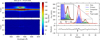 |
Fig. 1 Illustration of the extraction process for one of the exposures in the RED arm. Left: 2D reconstructed slit, before (top) and after (bottom) subtraction of the PSF models for both the primary and the companion. Right: illustration of the extraction process at a single wavelength bin within Hα. The blue- and green-shaded regions are the various Gaussian components used in the PSF fitting process for the primary and companion, respectively (three Gaussian components here for the RED arm). Bottom panels: modeling residuals. |
3.1.2 Residual contamination
Despite the apparent quality of the extraction in most epochs, we found the PSF to be slightly asymmetric, a feature reported in UVES’s manual. In fact, we found this asymmetry to vary between epochs. This led to a residual contamination of the primary in the companion spectrum, particularly during epochs with pronounced asymmetry. We note that we did not identify any correlation between seeing and PSF asymmetry.
Figure 2 shows, in the middle panel, one epoch where the companion spectrum is strongly contaminated by the star. This is apparent from the spectral features that strongly follow that of the primary (see Fig. B.1 for the full primary spectrum). As a post-processing step, the residual contamination was subtracted by fitting the companion’s local continuum with the primary spectrum, and an offset that accounts for both the contrast and the baseline continuum shape.
The contamination in each exposure was modeled as
 (1)
(1)
where
F(λ) is the extracted spectrum of the companion for that exposure,
P(λ) is the spectrum of the primary for that exposure,
M(λ) is a master spectrum of the companion computed as the average of the epochs that are least affected by contamination,
k is a general scaling factor to account for that exposure’s calibration,
α(λ) is the contamination factor from the primary to the companion.
The algorithm solves for k and α(λ). Because it involves both a general scaling factor (k) and a wavelength-dependent parameter (α(λ)), the fit was performed simultaneously on all wavelength bins. Each α(λ) was computed by solving the equation within a ±5000 km/s window centered on λ.
The fit was performed using scipy’s implementation of the limited-memory Broyden–Fletcher–Goldfarb–Shanno (L-BFGS-B) algorithm (Byrd et al. 1995; Zhu et al. 1997; Virtanen et al. 2020). To avoid over-fitting noise features, the final α(λ) parameter was smoothed with a Gaussian kernel on a 10 px window (see Fig. 2, first panel, red line). The 1σ error bars were computed by setting k to the best fit value, and computing the  map for all α(λ) values. Then, the
  contours served to compute the location of 1σ error values on the α(λ) parameters. This was performed independently at each wavelength. The error bars are shown as the shaded region in Fig. 2, first panel.
The resulting contamination-free spectrum is shown in Fig. 2 (second panel, in green), following subtraction of the contamination component (red) from the extracted spectrum (black). The contribution of the contamination to the emission lines is shown in the last row of Fig. 2.
Contamination correction was not applied below ∼3700 Å due to the UV excess of the companion, which introduces significant continuum variability that the master spectrum M(λ) cannot reproduce. This does not have a significant impact on the results as the contrast between the primary and the companion is much better at these wavelengths, which translates into a minor contamination relative to the companion intrinsic flux. It should also be noted that while the contamination factor error bar increases at lower wavelengths, this is only because the flux of the binary decreases. The “true” error on the contamination stays mostly constant, but the error bar on the contamination factor increases to make up for the decrease in binary flux.
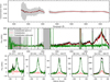 |
Fig. 2 Illustration of the residual contamination correction for the exposure 2022-11-05 UT 01:22:25. This corresponds to the case with the highest contamination. Top panel: residual contamination factor (black) smoothed with a 10 px wide-moving Gaussian box (red) and its associated error bars (black-shaded region). Middle panel: companion spectrum as the output of the extraction process (black) with the contamination contribution (red) and the contamination-corrected companion spectrum (green). All black-shaded regions were excluded from the fit; they correspond to emission lines and detector edges. Third row: contamination contribution within emission lines (same colors). The contamination removal process is able to remove most of the residual primary flux in the companion spectrum, which accounts for ∼10% of the lines flux depending on the exposure. |
3.2 Absolute flux and spectral calibration
All spectra were corrected for barycentric velocity (BERV) at the time of observations and for the radial velocity of the Delorme 1 system. We used the radial velocity shift of 7.3 ± 2.6 km/s (Kraus et al. 2014). As the orbital velocity of Delorme 1 (AB)b is unknown, we did not correct for it. However, at its projected separation (88 AU), and given the mass of the central binary, even if the planet was seen along its orbital plane, the Keplerian velocity for a circular orbit would be at most ∼2 km/s.
The slit width (0.8′′) of UVES can lead to slit losses depending on the seeing. However, the binary is known to display very little flux variability, both in the NIR (∼3%; Bowler et al. 2023, their Fig. 20) and in the optical (Gaia DR3, ∼1%; Gaia Collaboration 2018, 2023) and therefore provides a reliable baseline for flux calibration of the companion spectra. We therefore normalized all spectra of the binary to the same flux level around Hα to construct a mean spectrum of the binary, which was then scaled to the Gaia DR3 GBP magnitude (GBP = 15.690 ± 0.005 mag) to provide a spectro-photometric calibration of each individual epoch. The GBP filter is only slightly broader (by ∼50 Å) in the near-UV part but benefits from multiple epochs of observations obtained at a high accuracy level, making it particularly suitable for absolute flux calibration.
There are no apparent discrepancies between the spectral slopes of the spectra of the primary, as shown in Fig. B.1 from one epoch to the other. There are no correlations between the spectral slope, seeing, air mass, or other observational parameters (note that the air mass correction is automatically performed by the pipeline), which implies no strong systematics from epoch to epoch. We also find a good match between the binary mean spectrum and the spectra of young pre-main-sequence stars from Manara et al. (2013b) (Appendix G) supporting the lack of significant bias in our data.
The spectra of Delorme 1 AB are globally consistent with flux densities corresponding to published APASS B, SkyMapper v, SDSS g, APASS V, and SDSS r magnitudes of Delorme 1 AB (Henden et al. 2016; Onken et al. 2024; Abdurro’uf et al. 2022) converted to flux densities using the VOSA tool (Bayo et al. 2008) and SVO Filter Profile Service (Rodrigo et al. 2012; Rodrigo & Solano 2020). We find a slight shift in the APASS B and SkyMapper v photometry with respect to the flux level of the BLUE arm spectra. However, we refrained from using that photometry for additional corrections because the star is either accreting or active – and that photometry might be variable as well (especially given that the Gaia GBP filter spans a broader wavelength range and is more stable across epochs).
The mean MUSE spectrum of Delorme 1 AB published in Eriksson et al. (2020) is significantly brighter than the whole set of reference photometry and our spectra. More details on the comparison can be found in Appendix G.
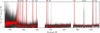 |
Fig. 3 Final spectra over the full spectral range. All Delorme 1 (AB)b spectra, overlaid in black, with the mean spectrum in red. All spectra were smoothed to R = 5000 for clarity. The UV excess of Delorme 1 (AB)b is clearly visible below ∼3700 Å, as well as the generally flat continuum shape. The line marked as an artifact is due to a bad-pixel row on the detector. |
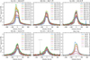 |
Fig. 4 Balmer lines of Delorme 1 (AB)b. Each panel shows the mean line of each observing epoch (11 epochs), from Hα to Hϵ. The last panel shows the mean line (over all epochs) for each transition order up to Hθ/H10. All lines were plotted after subtracting the local continuum baseline, averaged between (−750;−400) and (+400;+750) km/s. The lines show great profile and amplitude variability across epochs. |
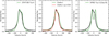 |
Fig. 5 Comparison of the mean Hα line profile of Delorme 1 (AB)b to that of two young substellar objects with disks (left: CFHT BD Tau 4, center: ChaHa-1) and of a Class III 15 MJup brown dwarf (right: KPNO Tau 4). We scaled (in red) the profile of Ca Ha 1 to the free-fall velocities expected for Delorme 1 (AB)b. The profiles are similar to that of CFHS BD Tau 4 and ChaHa-1, but not to that of KPNO Tau 4. |
4 Results
4.1 The spectrum of Delorme 1 (AB)b
The derived spectrum of Delorme 1 (AB)b is shown in Fig. 3, with all epochs overlaid in black and the mean smoothed spectrum (R=5000) in red. The mean spectrum of Delorme 1 (AB)b resembles that of SR 12 c, a young (∼2 Myr) companion with a similar quoted spectral type (XSHOOTER; Santamaría-Miranda et al. 2018; Santamaría-Miranda et al. 2019). We find that Delorme 1 (AB)b has a Gaia GBP magnitude of GBP=20.6 ± 0.2. It should be noted that the apparent spread of the black-shaded region only represents the S/N of individual spectra. The noise is much higher in the BLUE arm (lower wavelengths) than it is in the RED arm (higher wavelengths). Continuum variability is observed (see Sect. 5.3.2), but it is not obvious at R = 5000 in Fig. 3.
A UV excess is evident at wavelengths below ∼3600 Å (Fig. 3). In T Tauri stars, UV excesses are believed to originate from the accretion shock at the object surface. Such a feature is commonly interpreted as a signpost of ongoing accretion (Valenti et al. 1993; Gullbring et al. 1998; Herczeg & Hillenbrand 2008; Ingleby et al. 2013; Hartmann et al. 2016).
Only a handful of PMCs have shown detectable UV excesses to date (Zhou et al. 2014; Zhou et al. 2021).
4.2 H i Balmer emission lines
All Balmer lines of Delorme 1 (AB)b can be found in Fig. 4 and lines of the host binary are shown in Fig. B.2. The Hα, Hβ, Hγ, and Hδ line profiles for each individual exposure (companion only) can be found in Figs. C.1, C.2, C.3, C.4, along with the standard deviation of the lines around the mean line. The integrated line fluxes are given in Table C.1.
While higher-order lines are quite symmetrical, the Hα and Hβ lines have asymmetrical profiles with extended wings (up to ± 500 km/s) and a core with a tilted plateau profile. Although this could reflect partial saturation in the line emission, we instead explain it through a two-component decomposition (see Sect. 4.5). This plateau is most tilted on epochs October 13, 14, and 15, 2022, and coincides with an extended blue wing seen on October 14 and 15. This epoch coincides with an outburst of accretion, as seen from the increased UV excess flux at the same dates (see Sect. 4.5.3). The first epoch of our series (2021-10-25) corresponds to the one already published by Ringqvist et al. (2023). They had only presented the BLUE arm, which covers Hγ and higher order lines. Here, we introduce Hα and Hβ for the first time.
4.3 Comparison to free-floating objects
In Figure 5, we compare the Hα line profiles of substellar accretors from Mohanty et al. (2005) and Muzerolle et al. (2005) to the mean Hα profile of Delorme 1 (AB)b. The plateau of the Hα profile of Delorme 1 (AB)b closely resembles those of CFHT-BD-Tau 4 and Cha Ha 1, two young (1–3 Myr) brown dwarfs with estimated masses of 60 MJup and 35 MJup, respectively (Fig. 5). The core of CFHT-BD-Tau 4’s line is also comparable to that of Delorme 1 (AB)b while Cha Ha 1’s is noticeably broader. We rescaled the profiles of Cha Ha 1 to match the expected free-fall velocities of Delorme 1 (AB)b assuming a similar inclination of the two objects. A rescaling by a factor of 0.8 provides the best fit (corresponding to a mass of 20 MJup). However, the wings of Delorme 1 (AB)b are still more extended, in particular on the blue side of the line. Both objects have clear infrared excess, as identified by the VOSA spectral energy distribution (SED) analyzer (Bayo et al. 2008).
We also show in Fig. 5 the profile of the 15 MJup brown dwarf from Taurus KPNO Tau 4. The object is known to be devoid of infrared excess (Bonnefoy et al. 2014). As such, it is the only class III object in the mass range of Delorme 1 (AB)b with profiles available at a resolution close to UVES. It displays a double-lobe profile also retrieved in active M dwarfs (e.g., Short & Doyle 1998; Mohanty et al. 2005).
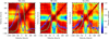 |
Fig. 6 Autocorrelations of the lines Hα, Hβ, and Hγ. The color indicates the value of the Pearson correlation coefficient. The lines were smoothed to R ∼ 40 000 to remove some of the noisy features. The lack of correlation between the wings and the core suggests that the lines may be made of two subcomponents. Overplotted in blue and green are the two subcomponent decompositions obtained in Section 4.5, explaining the features of the autocorrelation. The correlation diagrams for the higher order lines have the same overall shape as Hβ and Hγ. |
4.4 H i emission line autocorrelation diagrams
Figure 6 shows the autocorrelation (Pearson coefficient) diagrams for (Hα, Hβ, and Hγ). Overplotted in blue and green are the respective two-components decomposition for the line (see next Section 4.5). While autocorrelation diagrams are commonly used in studying time-series of accretion lines in T-Tauri stars (e.g., Alencar et al. 2012), we extend their usage to the planetary-mass regime. Autocorrelation diagrams represent the Pearson correlation coefficient between different velocity channels of the lines. They help show how different parts of the lines evolve with respect to each other. They have been used, for example, as a means to hint at the magnetic field topology, by comparing observed autocorrelation matrices to those predicted from magnetohydrodynamics (MHD) simulations (Alencar et al. 2012).
In all three lines, the core and wings of the profiles appear uncorrelated over a central region ∼50 km/s wide. Hα shows an additional uncorrelated region around ∼60 km/s. This may be interpreted as the Hα line being likely composed of up to three independent components (wings, core, and ∼60 km/s component), while Hβ and Hγ are likely formed of two components. It remains unclear whether the ∼60 km/s component belongs to the core or wing structure, or constitutes a distinct third component. Alternatively, correlated velocity channels may originate from different physical regions but still have common evolution.
In the case of Hβ and Hγ, the correlation coefficient between the core and the wing reaches ∼0, which means both components are completely independent. However, for Hα, the correlation coefficient between the core and the wings only reaches a minimum of 0.5. This implies that if Hα’s core and wing components were truly independent (as seen in Hβ and Hγ), the contrast between the components should be lower than for Hβ’s or Hγ’s.
4.5 Decomposition of the H I line profiles
Emission line profiles are usually decomposed as multiple Gaussians (e.g., Ringqvist et al. 2023; Viswanath et al. 2024) that can trace different emitting areas or mechanisms. However, most recent accretion models indicate that the line profiles should deviate significantly from Gaussian shapes when complex emitting regions are involved or coexist. While shock-emitted lines have a more symmetrical profile (Aoyama et al. 2018) that Gaussians may be able to reproduce, lines emitted in a magnetospheric accretion funnel tend to be affected by complex absorption features (Thanathibodee et al. 2019a). Alternatively, the lines may also originate from a mixture of accretion and chromospheric activity (e.g., Thanathibodee et al. 2020).
Due to the complex shape of the autocorrelation diagrams (Fig. 6), we chose to retrieve an empirical decomposition of the lines that does not assume Gaussian components. We developed a custom method based on the L-BFGS-B algorithm to disentangle multiple components within the lines. This approach was made possible by the large volume of time series data available. The method is described in Sect. 4.5.1, and the results in Sects. 4.5.2 and 4.5.3.
4.5.1 Method
We developed a novel method to decompose the lines into multiple components. This method makes no assumption as to what shape these components should have and effectively infers the components that best reproduce the observed profiles across all epochs and exposures.
Using the fact that multiple components of a line may be related to different emitting mechanisms, we made the following two assumptions: (i) each line is the sum of multiple emission components of arbitrary shape. (ii) The shape of each component does not vary between exposures, only their relative amplitude does. This assumption physically corresponds to distinct emitting regions that would have negligible variability in their respective line profile. In the following, we set the number of components to two, as additional components would have the algorithm jump between multiple local minima. We also tried adding an absorption component (corresponding to an absorption region on top of an emitting region), but this did not improve convergence.
The model treats the observed flux F(v,t) as a linear combination of velocity-dependent components scaled by exposuredependent factors, (Ci(v), ki(t)), such that the total line model is
 (2)
(2)
where Ci(v) is the value of the component i at the velocity v and ki(t) is the scaling parameter for the component i at exposure t. The fit is performed iteratively by solving for the values of C(v) for one of the components and k(t) for both components. The Ci(v) are alternatively solved for each component along the iterations. At each iteration, a fit was performed using Scipy’s implementation of the limited-memory L-BFGS-B algorithm (Byrd et al. 1995; Zhu et al. 1997; Virtanen et al. 2020).
The process did involve many free parameters, but this is still far below the number of data points that were actually involved in the fit. The total number of parameters is given by 2(2Nt+Nv), with Nt the number of exposures (33), and Nv the number of velocity bins (322 over (−250, +250) km/s). This yields a ratio of data-to-parameters equal to 13.7.
While the decomposition was performed using a flat prior for the shape of the components, we did try different initial guesses for the shapes. We find the results to be insensitive to the choice of initial parameters. This confirms that the local minima in the parameter space (if they exist) are all located within proximity of each other, with only slight deviations to the profile of each component.
We also investigated an alternative decomposition based on nonnegative matrix factorization (NMF), used by the direct imaging community to build PSF models. We retrieve decompositions of the Hα profiles close to the ones achieved with our method, and the results confirm the L-BFGS-B two-component decomposition, although with some slight differences (see Fig. E.1 for a comparative discussion of the two methods). However, the NMF requires all data to be positive, which is not verified at low S/N and requires excluding the faint wings of the lines, in particular in higher order lines (e.g., Hγ and higher). Therefore, we adopted in the following the decomposition gathered from our custom method.
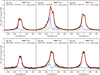 |
Fig. 7 Illustration of the decomposition for three different exposures for Hα (first row) and Hβ (second row). The two components are shown in blue and green, the total model in red, and the corresponding data in black. The decompositions for all exposures are shown in Figs. C.1, C.2, C.3 and C.4 for Hα, Hβ, Hγ, and Hδ, respectively. This decomposition provides a great fit to all exposures despite the strong constraint of a constant profile. |
4.5.2 The shape of the two subcomponents
The final decomposition for Hα and Hβ is shown in Fig. 7 (blue and green lines) for three different exposures. The shape of both components at the end of each iteration is shown in Fig. D.1 with transparent lines (blue and green). Each panel corresponds to the results of the decomposition of Hα, Hβ, and Hγ for the October 15, 2022, epoch at 06:30:49 UT. The results for all epochs are presented in Figs. D.2, D.3, D.4 and D.5. Due to the respective contribution of the two components within the wings and the core of the line, we hereafter call them “wings” (blue) and “core” (green) components.
The wing component rapidly converges within a few tens of iterations to a stabilized shape with deep absorption features, broadly centered at ∼15 km/s for Hα, and ∼3 km/s for Hβ, Hγ, and Hδ. The second (green) component converges to a narrow asymmetric profile centered on zero velocity.
The two components are shown overlaid on the autocorrelation diagrams in Fig. 6. For Hα, the core component correlates almost perfectly with the core component from the autocorrelation, as well as the reduced correlation in the 50–100 km/s range. The correlated wings are attributed to the wing components. The reduced correlation between −50 and 0 km/s corresponds to the blending of the wing component peak with the green wing. The double-peaked feature explains the correlation peak at ∼40 km/s in the autocorrelation diagrams. This wing profile is explained by magnetospheric accretion components (see Sect. 5).
Both Hβ and Hγ autocorrelation shapes are perfectly explained by their two-component decomposition as well. Similarly to Hα, the uncorrelated core and wings are explained by the two independent components. Their blue wings have a stronger autocorrelation than their red wings, which is explained by the shape of the wing component: its blue wing is brighter than its red wing. This asymmetry enhances contrast between the wing and core components, increasing the correlation strength in the blue wing.
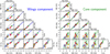 |
Fig. 8 Correlations between the wing and core components over multiple lines (Hα to Hδ), the mean continuum level (cont) around Hα (in 10−17 erg/s/cm2/Å), and the mean level of the UV excess (in 10−17 erg/s/cm2/Å). The Pearson correlation coefficient is given as text in each panel. The dashed black line is the y=x line. The blue and green lines and shaded regions are the best affine fit. The color coding of the data points is the same as in Fig. 4. The x and y units are normalized scaling factors of each component. The epoch on October 13, 2022, (orange) was excluded from the analysis because it is so far off the correlation in the core Hα component. The wing and core components are strongly correlated. However, only the wing components have a strong correlation with the UV excess, which could be due to accretion. The wing component and the UV excess are both strongly correlated with the continuum level around Hα, which suggests that the apparent continuum is veiled by the extension of the apparent continuum. |
4.5.3 Correlations between subcomponents
The insets in Fig. D.1 show the correlations between the scaling factors of the wing and core components. Observations from October 14, 15, and 17, 2022, correspond to brighter emission lines possibly tracing an outburst and are plotted as crosses. In Hα, the wing and core component amplitudes are strongly correlated, except during this “outburst” epoch, which corresponds to a strong wing component. Still, the wing and core components remain correlated during the outburst. However, Hβ, Hγ, and Hδ exhibit weaker correlation between their wing and core components; nevertheless, the outburst epoch consistently corresponds to a brighter wing component.
Figure 8 shows the correlation of each component (wings or core) across different lines, with Pearson correlations labeled in each panel. Both components are well correlated from one line to another. The mean flux level around Hα(500−5000 km/s on each side of the line) and within the UV excess (mean flux level in the 3350−3600 Å range) are also shown.
The continuum level around Hα (Fig. 8, last row, last column) is strongly correlated with the UV excess. This hints that the apparent continuum may instead represent a blend of atmospheric emission and veiling extending at these wavelengths. The wing components are strongly correlated with both the continuum level (around Hα) and the UV excess level (p∼0.90 in all panels). The core components, however, are only slightly correlated with the continuum and UV excess (p∼0.4), except for the Hα line (p∼0.65).
Given the similarity of the shapes of the wing and core components from one line to another, the correlations are not necessarily surprising. However, since the Hα line profile is distinct from that of other lines, it was not so evident that its subcomponents (both wing and core) would be so strongly correlated from one line to another. Still, this hints at a common mechanism for the wings (blue) components of all lines, and core (green) components of all lines.
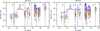 |
Fig. 9 Variability diagrams of Hα (left) and Hβ (right) relative flux for all pairs, as a function of the timescale, following the same method as Demars et al. (2023). We show the variability amplitude of the wing (blue) and core (green) components and of the total profile (dark red). The error bars represent the spread of the variability within a given timescale bin, weighted by the significance of the measurement: the σ-distance between the two lines corresponding to the measurement. Higher order lines have variability diagrams similar to that of Hβ, with slightly increased variability amplitude at hours timescales (see Fig. 10). The full-line variability amplitude is driven by that of the core component, because it contains most of the line flux, whereas the wing component is quite faint in comparison. |
4.5.4 Limits to the decomposition
Although the method described here provides a decent fit to the line profiles, residuals are clearly observed in Figs. D.2–D.5. The residuals have either a single or a double-peak feature. These residuals might be the sign of variable-shape components, missed by our method.
It should be noted that both the highest and the smallest residuals surprisingly appear within and around the outburst epoch. The strongest residuals are observed on epoch 2022-10-13, which precedes the outburst epoch, while the smallest residuals appear within the last two exposures of epoch 2022-10-15. These two exposures are taken an hour after the initial two, indicating that variability in the line profile likely occurs on timescales shorter than one hour. In fact, the wing component flux on that epoch are comparable to that of non-outburst epochs, while also appearing as an outlier in the correlation plots in Fig. 8. We find in Sect. 5 that the wing component is very likely due to magnetospheric accretion, a scenario in which line profiles are intrinsically variable. Therefore, the residuals are likely due to the intrinsic profile variability of the wing component, which is missed by our static components approach.
4.6 Line variability
All lines present profile and amplitude variability across epochs with minimal variability within individual nights. Figure 9 shows the variability of the line flux of Hα and Hβ as a function of timescale: all possible line-pairs were associated with their relative flux ratio (normalized to the fainter of the pair) and the time-difference between the two observations. This follows the same methodology as Demars et al. (2023) and is similar to that of Costigan et al. (2014) and Zsidi et al. (2022). The blue and green points correspond to the subcomponents evidenced in the previous Section, while the brown points correspond to the full line. The yearly timescale is driven by the 2021 October 25 epoch presented in Ringqvist et al. (2023). Figure 10 shows the variability amplitude on the hourly timescale, i.e., the shorter timescales in Fig. 9 and with the same color-scheme. Notably, the wing component has greater relative variability than the core one.
Both Hα and Hβ exhibit low variability amplitudes at hourly timescales (∼8%) and reach a near-plateau from days to months timescales. Higher order lines have variability diagrams similar to that of Hβ (not shown here) at timescales longer than a day. In contrast, Hα shows several peaks in variability amplitude, in particular slightly below the monthly timescale, likely driven by the blueshifted “outburst” on 2022 October 14, 15, and 17 (see Fig. 4). This is linked to the increased amplitude of the wing (blue) component.
The core component has a variability amplitude of a few tens of percent and a shape that is mostly in line with the overall profile, except for the monthly timescale where its amplitude is smaller. It makes sense given that this timescale is driven by the burst epoch, reflecting the increased importance of the wing component. However, the wing component has a variability amplitude that is greater (a few hundred percent) than both the core component and the overall profile, at all timescales, as is the case for all lines. This is mostly due to the almost complete disappearance of the wing component in some epochs, consequently amplifying the spread of variability relative across epochs.
The variability amplitude at hourly timescales seems to increase with the line transition order (see Fig. 10). This trend is absent at longer timescales. This is broadly consistent with the much higher variability amplitudes seen at the hourly timescale in Paβ for GQ Lup b and GSC 06214-00210 b (∼50%, Demars et al. 2023).
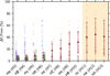 |
Fig. 10 Variability of the Balmer lines at the hourly timescale. The color of the points represents the component (blue for wings and green for core) or the full line (brown). Error bars represent the spread of the variability (weighted by significance), i.e., the brown crosses in Fig. 9. The shaded region corresponds to lines where the detection is compatible with contamination from the host binary. The hourly timescale variability seems to increase with the order of the transition. The wing component has a much higher variability amplitude than the green component. |
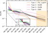 |
Fig. 11 Line ratios decrements. For each line, the line ratio is computed with respect to Hβ (H4). In black, the line ratios of the full-lines in this study are shown. Colored lines correspond to the four decrement types identified in Antoniucci et al. (2017) (see their Fig. 3). Blue and green lines represent the subcomponents (wing and core) obtained in Sect. 4.5. The shaded region corresponds to the lines, which may result from contamination from the host binary (as in Fig. 10). The full-line decrement (black) is broadly compatible with Type 2 case (optically thin emission and low accretion rate). The wing component is not clearly compatible with any decrement type. However, the core component is compatible with the Type 3 sources, which are not easily reproduced by emission line models (Antoniucci et al. 2017). |
4.7 Line ratios
Figure 11 shows the H i line ratios (all lines normalized to Hβ) of the full profiles (in black), as well as for the wing and core subcomponents. The typical line ratios found in T Tauri stars (Antoniucci et al. 2017) are also shown. Their study focuses on line decrements in the Lupus region (∼3–4 Myr), for a sample of 36 stars with masses in the range 30 MJup−1.5 M⊙, with only 4 objects below 100 MJup. They identify four classes of decrements. The lowest accretion sources in the sample show mostly Types 1 & 2 decrements.
The overall line ratios of Delorme 1 (AB)b (black lines) are consistent with the general trend of Antoniucci et al. (2017) decrements but they are not a perfect match to any of the four classes. They appear most compatible with the Type 2 case, which corresponds to optically thin emission and low accretion rate sources in Antoniucci et al. (2017). Surprisingly, the Hα/Hβ ratio, with values ranging from 1 to 3, is consistently below all of the T Tauri classes. We also note that our Hα/Hβ ratios are inconsistent with the one obtained from MUSE/VLT on October 18, 2018 (Hα/Hβ=9.8; Eriksson et al. 2020). However, the MUSE data are also incompatible with the published photometry of the primary, suggesting that they may suffer from residual bias.
The line decrements of the wing component display a more dispersed behavior across epochs, likely due to the faint emission level of that component in Hγ and Hδ. However, the core component shows lower dispersion and resembles the decrement profile of Type 3 sources from Antoniucci et al. (2017), except for its Hα/Hβ, which remains significantly lower than all classes. Antoniucci et al. (2017) mentions that Class 3 decrements cannot be well reproduced by the line emission processes (their Case B: optically thin emission and the local excitation model developed by Kwan & Fischer (2011) for radial flows around young stars) and remain the most difficult to interpret. The observed differences could reflect the complexity of the line-emitting region.
5 Comparison to models
We investigate two different H i line formation scenarios: 1) formation in magnetospheric accretion columns and 2) formation in a shock front. These two mechanisms are not mutually exclusive and may contribute simultaneously to the observed emission. We use the magnetospheric accretion models from Thanathibodee et al. (2019a) and the shock models from Aoyama et al. (2018). Magnetospheric accretion models are available for both Hα and Hβ, while shock models are available up to Hδ.
The analysis is similar to that of Demars et al. (2023) for the Paβ line of GQ Lup b and GSC 06214-00210 b. The line profiles are fit with the two models for both Hα and Hβ, while Hγ and Hδ are only fit with shock models. For both lines, the wing component has deep absorption features reminiscent of that from infalling material (e.g., an accretion column). The core component, however, has no obvious feature that could help discriminate between the two models.
5.1 Magnetospheric accretion models
5.1.1 Model description
The model assumes that the planet has an aligned dipolar magnetic field strong enough to truncate the disk. The H i lines form in the axisymmetric funnel flow following the closed dipolar magnetic field lines connecting the disk to the central object.
The parameters of the model are given in Table 1. Respectively, they correspond to the inner truncation radius (Rin), width of the column (width), accretion rate (Ṁ), column temperature (Tcol), inclination of the system (i), planet mass (Mp), radius (Rp), and effective temperature (Teff). Only a single value of Teff = 1800 K is considered as it mostly affects the continuum level within the synthetic lines, which was subtracted before fitting.
It should be noted that geometrical parameters are given in terms of planetary radius, and the planet radius mostly serves as a scaling parameter for the truncation radius and column width. They should therefore not be interpreted as a robust determination of the planet mass or radius. These may also serve as scaling parameters for the location and intensity of various absorption features. This is the case in particular for parameters with low sampling rates, for example the inclination, which is only sampled in 15∘ increments.
Parameter ranges for the magnetospheric accretion models (Thanathibodee et al. 2019a) and best-fit results.
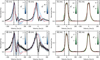 |
Fig. 12 Modeling results for the magnetospheric accretion models (Thanathibodee et al. 2019a). Left: results for the wing subcomponent. Right: results for the core subcomponent. First row: Hα. Second row: Hβ. Each left subpanel corresponds to the fit performed on the [−50; +50] km/s range, while the right subpanels correspond to the fit on the full the line width ([−250; +250] km/s). The red line is the best model, while the colored lines represent a sample of the lowest |

5.1.2 Modeling method
The synthetic lines sometimes have absorptions that extend below the continuum, which makes sense in the context of classical T-Tauri stars (CTTS). However, the models cannot reproduce the line flux of our observations, where the continuum is barely visible. We therefore subtracted the photospheric contribution from the models using a linear fit on either side of the line. This approach introduces negative values where modeled absorptions exceed the photospheric continuum. We therefore excluded negative values from the fit to mitigate this issue. We also normalized the lines to 1 around ∼0 km/s and focused solely on fitting the shape of the line components.
As done by Demars et al. (2023), the fits were performed by computing the  over the whole grid. The modeling was carried out over both the full line width and the core region, as the key features (wings and central absorption) are reproduced differently depending on the velocity range considered. The wing and core components are modeled independently. The best fit models, for both Hα and Hβ, are shown in Fig. 12. The
  parameter space is shown in Appendix F.1, along with a sketch of the best fit models. Table 1 shows the parameter values of the best fits.
5.1.3 Hα modeling
As shown in Fig. 12, the models are able to reproduce the absorption features in the wing component (blue), when fitting both the core and the full line. However, the best-fit model appears to yield a much narrower magnetosphere in the full-range fitting than in the core-fitting. This is explained by the degeneracy between the accretion rate and the column width seen in the full-range fit (Fig. F.1): a higher accretion rate with a wider column broadly yields a similar column density, with similarly shaped absorption features. Both the core and full-line cases broadly yield two minima: a low accretion rate with high column temperature, and a high accretion rate with low column temperature (Figs. F.1). Both the core and full-line profile types yield high inclinations, in the 60–75∘ range.
When fitting the core (±50 km/s) of Hα’s core component, the model reproduces the blue wing, but not the red wing tail. However, when the fit is extended to the full range of velocities (±250 km/s), the red wing is reproduced, but the main peak of the line is slightly narrower than the data. In this case, the blue wing is not reproduced by the model. In both cases, the modeling of Hα’s core component yield magnetospheres that are relatively thin. However, the core-fit yields a large truncation radius, while the full-line fit yields a low truncation radius. This difference might also be explained by degeneracies between multiple minima at truncation radii of 1.5 RJup and 3.0 RJup. The core and full-range modeling yield different inclinations: ∼30∘ for the core-fitting, and ∼75∘ for the full-range fitting.
5.1.4 Hβ modeling
Hβ’s wing component exhibits very different behavior. Models can reproduce the dip at the core of the lines when the fit is performed from ±50 km/s but fail to capture the wings simultaneously. Conversely, the fit on the larger velocity interval (±250 km/s) reproduces the wings, but not the central absorption. In fact, some of Hα’s best models also display similar behavior, as shown by some of the blue-shaded profiles. Both fits of Hβ yield magnetospheres with similar extents and mainly differ in terms of accretion rates and column temperature. However, the  maps show that when the line core alone is fit (±50 km/s), the magnetosphere geometry remains poorly constrained. The accretion rate and column temperatures are also highly degenerate. When the full profile is fit, the geometry is best reproduced with a small launching radius and large column width, but no constraints on the inclination are derived.
Hβ’s core component has a similar behavior to that of Hα, when considering the fit over the wide and narrow velocity intervals. When modeling the line core, the width of the line is well reproduced, as well as its red wing, but not its blue wing. The slope at the top of the line, however, does not match that of the data. In the full-line modeling case, both wings are fairly well reproduced, along with the width of the line. The magnetosphere extent is similar in both cases and is in agreement with that of Hα’s: a narrow and compact funnel. It is, however, slightly degenerate with a wider and extended magnetosphere. The inclination differs slightly between the core and full-line modeling cases. The core-fitting yields two inclination minima, one at low inclination (<30∘) and one at high inclination (75∘). This degeneracy is lifted by the full-range modeling, which favors a highly inclined system. The column temperature and accretion rate are in both cases degenerate between two regimes: low-Ṁ/high-Tcol or high-Ṁ/low-Tcol, the same trend that is observed for Hα’s core component.
5.2 Shock models
Despite the small correlation factor of the core components with the UV excess, their shape resembles that of the prediction from Aoyama et al. (2018) accretion shock models. However, the models do not predict lines similar to the wing component. Therefore, we only considered the core component for the fit.
5.2.1 Model description
The shock model includes two free parameters: the infall velocity, v0, and the post-shock density, n0. An additional parameter, the shock surface, is introduced as a scaling factor for the line intensity. Since the core component varies only in intensity and not in shape, the shock surface is the sole epoch-dependent parameter. As with the magnetospheric accretion models, we compute the  value across the entire parameter grid.
5.2.2 Core component modeling
Figure 13 shows the best fit models to the core components of Hα to Hδ, along with the  space. Figure 14 shows the accretion rate computed from the models, depending on the epoch. The accretion rate is computed using the relation Ṁ=S μ′n0v0, where μ′ = 2.3 × 10⁻²⁴ g is the mean molecular weight per hydrogen nucleus and
  is the emitting area given the filling factor ffill (Aoyama & Ikoma 2019; Aoyama et al. 2020). We assume a planetary radius Rp = 1.5 RJup. The best-fit parameters are given in Table 2.
For Hα, the models broadly reproduce the width of the line and the red-wing asymmetry. The central feature is too broad to fully match the line peak. However, the model does reproduce the flat-topped line observed in the data. The best models are those for v0 ∼ 120 km/s and n0 ∼ 1019 m−3, which are slightly degenerate with v0 ∼ 150 km/s and n0 ∼ 1018 m−3.
For Hβ, Hγ, and Hδ, the core components are much more symmetrical, which are well matched by the shock models, as shown by the corresponding  values. For all three lines, however, the blue side of the line is consistently underestimated, while the red side is well fit. All three lines have a preference for high infall velocities v0 > 180 km/s. Hβ fits at n0 = 1019 m−3, similar to Hα, while Hγ and Hδ fit at n0 = 1020 m−3. Both Hγ and Hδ converge near the grid limits, a trend also noted for the Paβ line of GSC 06214-00210 b (Demars et al. 2023).
As shown in Fig. 14, the accretion rate inferred from the core-component modeling varies between lines. They follow a consistent ordering: Hδ > Hγ > Hα>Hβ. Accretion rates derived from Hα and Hβ are compatible with each other within 1 σ, as are Hγ and Hδ. The Ṁ obtained from Hα modeling is systematically higher than that of Hβ, despite its lower n0 (1019 vs. 1020 m−3). This is due to the larger effective shock-surface, as highlighted by the values of ffill shown in Table 2. ffill(Hα) is on the order of ∼1%, whereas ffill(Hβ) is on the order of ∼0.2%. Hγ and Hδ are approximately half that of Hβ: ffill(Hγ) ∼ ffill(Hδ) ∼ 0.1%. Although all values are compatible within 3σ, the systematic ordering across epochs hints at a persistent bias. It may be due to the model, or to the flux calibration, which remains challenging to achieve with UVES. However, Hγ and Hδ are located at nearby wavelengths (4341 and 4103 Å) and therefore within a single detector and arm of UVES, which makes relative calibration errors unlikely.
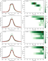 |
Fig. 13 Modeling results for the shock models (Aoyama et al. 2018), with the flux scaling corresponding to epoch 2022-10-14 – 06:52:50). On each row, the left panel shows the core component for that line (black line), a sample of the best fits (green lines) and the best fit (red line). Right panel: corresponding |

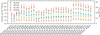 |
Fig. 14 Evolution of the accretion rate inferred from shock modeling of the core component, depending on the line. The accretion rate is computed as Ṁ=S n0v0μ. The right axis shows the corresponding Lacc = GṀMp/Rp, with Mp = 13 MJup and Rp = 1.5 RJup. The accretion rates inferred from different lines are systematically ordered, which may point to a bias from deriving accretion rates from a single line. |
5.3 Analysis of the UV excess with slab models
We modeled the UV excess as the emission of a slab of hydrogen following Manara et al. (2013a) under the assumption of local thermal equilibrium. To do so, we considered the X-shooter spectrum of the class III young M9.5 dwarf TWA29 (Manara et al. 2013b) as a template of photospheric emission for Delorme 1 (AB)b and fit simultaneously for visual extinction. To ensure a sufficient S/N, the modeling was performed on the mean spectrum of each night, at low spectral resolution (R ∼ 1000, convolved with a Gaussian kernel). The accretion luminosity (log(Lacc)) and accretion rate (Ṁ) derived from the models are reported in Table 3. All fits converged to AV = 0.
5.3.1 Comparison of Lacc and Ṁ
Figure 15 shows a comparison between accretion luminosities derived from slab-modeling (Lacc(slab)) and line fluxes (Lacc(line)), obtained with the relationships from Alcalá et al. (2017). The derived accretion luminosities from the slab model are broadly in line with those obtained from the wing component of all lines, and not consistent with those from the core component. This further highlights a strong connection between the wing component and the UV excess, whereas the core component is not correlated to the accretion shock, as shown by the correlations in Fig. 8. However, accretion luminosity derived from the wing component of different lines have different behaviors. Lacc(Hα) and Lacc(Hβ) are consistently below Lacc(slab), whereas Lacc(Hγ) and Lacc(Hδ) are consistently above Lacc(slab). This is in line with the findings of Alcalá et al. (2017) for stellar and substellar objects, where the average Lacc from all lines is in very good agreement with that obtained from the UV excess modeling, suggesting that the same phenomena may be at play.
The Lacc and Ṁ computed here are compatible with that obtained from modeling the wing components with magnetospheric accretion models. The slab modeling yields results of a few 10−12 M⊙/yr, which is consistent with wing-component modeling for Hα as well. For Hβ, however, the best fit results are obtained with higher accretion rates (∼10−(10–11) M⊙/yr). Still, the core-fitting of Hβ’s wing component is highly degenerate with much lower accretion rates, of a few 10−12 M⊙/yr, in line with the slab modeling. Yet the wings are only reproduced under higher accretion rate conditions. As for the core component, it consistently requires a high accretion rate and is therefore not compatible with what we find from the UV excess fitting. We find the same results with the computed Ṁ and Lacc from the shock-modeling (Fig. 14), which yield accretion rates an order of magnitude higher than those from slab modeling.
In summary, excess parameters derived from slab modeling align with those obtained from the wing components, from both empirical behaviors and magnetospheric accretion modeling. Instead, the core component’s corresponding Ṁ and Lacc are much higher than that from slab-modeling.
Core-component shock-modeling results (Aoyama et al. 2018).
UV excess best-fit results for the slab models.
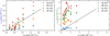 |
Fig. 15 Correlations between the accretion luminosity (Lacc) obtained from the UV excess fitting (slab-modeling) and the wing (left) and core (right) components fluxes (Alcalá et al. 2017). The black line shows the Y = X curve. The average accretion luminosity derived from the wing components of various lines is correlated with the accretion luminosity derived from that of slab-modeling (Sect. 5.3), while the accretion luminosity derived from the core component is well above it. |
5.3.2 UV and continuum variability
Figure 16 shows the best-fit slab-models for all epochs. While the UV excess is well reproduced, the model does not provide a good fit to the shape of the continuum. However, its general flux level is responsible for most of the fitted model. Below 6000 Å, the shock component is responsible for >60% of the continuum flux for all epochs except 2022-10-13 and 2022-11-01. Above 6000 Å, the shock component is responsible for 20−60% of the flux depending on the epoch. However, the exact observed shape still has some residuals that are most visible in the BLUE (<4500 Å) and REDL (4600–5700 Å) detectors.
The slab models are able to reproduce the height of UV excess (<3700 Å), but not the location of the jump itself. This is a well-known behavior as high-order Balmer lines blend near the true location of the jump, shifting its apparent location, while the slab model only accounts for continuum emission. The general shape of the continuum (4000–7000 Å) is not systematically reproduced by the models. The modeled UV excess appears to extend all the way up to Hα, and dominates over the photospheric contribution in most epochs. The best fits are for the outburst epochs (2022-10-14/15), where the residuals are only up to 25% for certain wavelengths, and average to 0 overall. In other epochs, the residuals go up to 50% in the RED arm, while the BLUE flux is not reproduced. Overall, even with the residuals, the results are consistent with the correlation observed between the UV excess level and with the continuum level around Hα (Fig. 8). This suggests that a fraction (if not most in some epochs) of the optical continuum on Delorme 1 (AB)b is actually due to the extension of the UV excess, which is strongly linked to the accretion rate.
The difference between our modeling and the data may have multiple origins. Espaillat et al. (2021) had used different slab components to account for the density structure of the accretion shock on GM Aurigae. They found the best fits are achieved with three shock components. It is possible that our assumption of a single shock component may prove to be too simplistic, possibly explaining at least the lack of flux in the models in the BLUE arm. Alternatively, our spectra may have residual spectral shape distortions, but the stability of the calibration to the host binary (see Fig. B.2) tends to suggest that the calibration should be fairly stable. It is hard to conclude whether the modeling or data should be improved. Still, the general conclusion remains that the UV excess extends to longer wavelengths, at least up to Hα(6564 Å) where we observe the strongest continuum variability.
6 Discussion
6.1 Line variability origin and impact
Eriksson et al. (2020) had already given a glimpse of the hourscale line variability of Delorme 1 (AB)b. Here, we explore timescales from hours to years for the first time for this object. The variability diagrams (Fig. 9) show that, similar to GQ Lup b and GSC 06214-00210 b, the variability at the hourly timescale is significantly smaller than at longer timescales. However, while GQ Lup b and GSC 06214-00210 b had non-negligible variability at the hourly timescale, the lines of Delorme 1 (AB)b only vary by a few percent (Fig. 10). Higher order lines do reach 10–40% variability, similar to that of the Paβ line of GQ Lup b and GSC 06214-00210 b. However, the line-flux variability is mostly driven by its core component, whereas the wing component does reach several ∼10% variability at Hα and higher transition orders. The wing component variability is responsible for the changing shape of the line profile, in particular with the excess seen in the outburst epochs of October 13-17, 2022. The general shape of the variability amplitude diagram is similar to that of GSC 06214-00210 b, which may hint at a common emitting mechanism.
Previous studies have proposed that line variability could explain the low detection yield of Hα imaging campaigns (e.g., Fischer et al. 2023). However, if Delorme 1 (AB)b properties are typical of most PMCs, its moderate variability range at the hourly (<∼10%) to the monthly (<∼ 50%) timescales seems insufficient to account for the low detection rates. The variability on the yearly timescale does reach factors of 2−3, but it is only driven by the 2021 epoch presented in Ringqvist et al. (2023), and might not represent the full variability at this timescale. Close et al. (2025) and Zhou et al. (2025) have studied the Hα line variability of PDS 70. Both found similar results, where the line varies by a factor of a few on yearly timescales, but never reaches a full order of magnitude.
Given the large sample of lines and epochs, we searched for periodicity in the data but found no statistically significant signal. In fact, any rotationally modulated effects that may be present at days-long timescales are lost to aliases inherent to the random time-sampling of the data (obtained in service mode without predefined time constraints). Future observations, if looking for rotational modulation of the lines, should focus on time-series of 4−5 hours over 3−6 days, as they typically cover the rotation periods of these objects, and the likely funnels that may periodically obscure the line of sight.
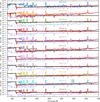 |
Fig. 16 Best-fit results to the UV excess and general continuum level using the slab models. The colored lines represent the individual mean epochs. The best fit components are shown for the UV excess (black, slab), photospheric template (light blue, class III), and total model (red). The data were smoothed to R ∼ 250; points below 20% the median level are masked; and a dashed line at 10−18 erg/s/cm2/Å is plotted at each epoch. All spectra are given in erg/s/cm2/Å units. The modeling provides a good fit to the UV excess and shows that almost all epochs have their continuum dominated by the shock-component extending to higher wavelengths. This is particularly evident in outburst epochs (2022-10-14/15). |
6.2 Origin of the H i Balmer lines in Delorme 1 (AB)b
6.2.1 Accretion origin: Wing component
Magnetospheric accretion emission models are able to reproduce the main features of the two Hα components. In higher-order lines, the models provide a great fit to the central absorption of the wing components, and are also able to reproduce its wings, although not simultaneously. Such features are strongly reminiscent of magnetospheric accretion profiles predicted when funnel flows intersect the line of sight to hot spots on the stellar surface.
The autocorrelation maps of Hβ and Hγ in Figure 6 are also qualitatively similar to the predicted maps from Alencar et al. (2012) based on the MHD simulations of magnetospheric accretion funnels launched from an inclined dipole from Romanova et al. (2011). Still, the ability of fixed-profile components to adequately fit all epochs suggests either a well-aligned magnetic dipole, persistent visibility of at least one accretion column, or a pole-on viewing angle for a more complex magnetospheric geometry. In the latter scenario, the whole observed variability would be caused by changes in the accretion rate and/or column temperature. However, observations of magnetospheres in T Tauri stars show that the dipole is usually moderately inclined with respect to the stellar rotation axis (McGinnis et al. 2020), and the modeling shows that both the wing and the core components are best reproduced by magnetospheric accretion models at intermediate to high inclination. The magnetosphere may still be axisymmetric, with models converging to high-inclination to simulate a non axisymmetric column seen at an angle. This may lead to substantial rotational modulation of the line profiles, if the magnetosphere were not axisymmetric. The identification of the rotation period of Delorme 1 (AB)b coupled with a determination of the v.sin(i) will be important to better constrain the models. In addition, a dense spectroscopic monitoring on timescales of the rotation period will be critical to further test the magnetospheric accretion scenario.
Overall, the wing component appears linked to ongoing accretion, based on both the model-fitting and its strong correlation with the UV excess, derived Ṁ and Lacc. Although the wing component has wings extending to velocities reminiscent of winds, no evident wind or jet tracers (e.g., OI lines) are detected, suggesting they are either absent or below the detection threshold. With broad values of accretion rate of 10−12−10−11 M⊙/yr, the planet would only accrete about 0.03−0.3 Mjup over its 35 Myr of age, suggesting that it is in the late phases of accretion, or that accretion may occur in bursts rather than a homogeneous process.
6.2.2 Accretion origin: Core component
The magnetospheric accretion models provide a reasonable fit to the core component, although there are no definitive absorption features as there are for the wing component. If the core component is in fact also due to magnetospheric accretion, it could not originate from the same emitting region. Thanathibodee et al. (2019b) proposed an onion-like funnel structure for the low-accretor CVSO 1335, where two funnels are launched from two different truncation radii. This scenario may explain the goodness of the magnetospheric accretion fits, as well as the relative shape of the two components. Thanathibodee et al. (2019b) also suggest that a companion in the accretion circumstellar disk may open a gap, causing two distinct accretion flows. Having a more complex magnetospheric accretion geometry would certainly better reproduce both the central absorption and the structures of the wing component of Delorme 1 (AB)b. The core component is seen in emission broadly where the wing component has its main absorption feature, which could be a sign of the relative projection to the observer of each emitting region. However, the physical parameters of the fits do not yield a core-component funnel that is strictly encapsulating the wing component funnel. This might be due to the simplicity of assuming an axisymmetric flow. Further modeling, for example with inclined dipole models, is required.
Alternatively, if the magnetospheric accretion scenario holds, at least for the wing component, the ability of magnetospheric accretion models to separately model the wings and the core of the line (Fig. 12) may also be explained by this onion-like structure. In this scenario, a line decomposition with three components might have unveiled the structure of the accretion columns. However, this was not done because a three-component decomposition would be too unstable (in an algorithmic, numerical sense) given the method described in Appendix E.
6.2.3 The shock scenario
The correlations between wing components and UV excess (Fig. 8) suggest that the wing component emission emerges only past a certain threshold level of the UV excess emission. Although it is possible that the correlation may not extend linearly to a zero origin, there are still data points very close to zero, for instance, the wing component of all lines on October 25, 2021. As for the core component, the correlation could similarly be interpreted as the UV excess requiring a certain threshold of core component emission for UV excess to appear. However, the poor correlation likely means that if the core component and UV excess emission are related, this is only to a moderate degree. Still, the width of the core component fits surprisingly well with shock models (Aoyama et al. 2018), and the retrieved parameters have an infall velocity (>170 km/s) compatible with that one might expect from magnetospheric accretion: shock at planetary surface (R ∼ 1.5 RJup) coming from a truncation radius of ∼10 RJup. This would suggest that the core component is in fact emitted at the shock, but then one might expect a strong correlation with the UV excess, as they would more-or-less trace the same region. Radiative transfer effects, such as optical depths or opacities, could be the explanation, but have not been modeled. While the wing component would be emitted in a broadly optically thin medium (the part of the accretion column close to the planet), the post-shock region emission could be saturated, explaining the plateau-like shape at the peak of the core component in low-order lines. This plateau diminishes with higher-order lines (Hβ, Hγ, Hδ), and increases the correlation with the UV excess, as is the case from Fig. 8, although this pattern breaks down for Hα’s core component, which shows stronger correlation with UV excess than the higher-order transitions.
While we did not try to fit any shock component to the wing component, it is also possible that part of the wing component may originate from a shock, which would not be surprising given its strong correlation with the UV excess. However, whether this component would be significant relative to the total line flux is difficult to confirm, and adding free parameters for a shock-column emission model would only accentuate the already existing degeneracies. Still, the wing component profiles are broadly reminiscent of that predicted by Marleau et al. (2022) for a shock-emission in a magnetospheric accretion scenario, when the column dust and gas opacities are included, although this was true for quite high accretion rates (>10−8 M⊙/yr) compared to the values we find in this paper.
Figure 16 shows that the continuum of Delorme 1 (AB)b seems to be modulated by the accretion shock. In fact, we find that the continuum level around Hα increases by a factor of ∼2.5 in outburst epochs (2022-10-15/15/17). This strong contribution of the UV excess to higher wavelength is consistent with the apparent over-luminosity of the source. Almendros-Abad et al. (2025) has recently identified a long-lived accretion burst in the free-floating PMO Cha1107-7626. They find that the flux levels around Hα increase by a factor of 3–6 within the outburst, which is on the order of magnitude of our findings. However, the duration of their accretion burst is much longer than what we see for Delorme 1 (AB)b (a few days). It is possible that our UVES observations were captured within an accretion burst similar to Cha1107-7626, and that the burst observed on 2022-10-14/15/17 is only a smaller modulation of a longer general variation. While the Hα shape variability observed in Almendros-Abad et al. (2025) is much different from that observed for Delorme 1 (AB)b, this may be due to different accretion geometry, viewing angle, or regime.
6.2.4 Unresolved binarity
The two components within the lines (wing and core) could also be caused by two tightly bound PMOs. The over-luminosity caused by binarity could have been left unnoticed in color-magnitude diagrams, since the color variation along the late-M early-L dwarf sequence is not strong, especially at NIR wavelengths. One tightly bound planetary-mass binary (2M0441) in Taurus has been identified as part of a quadruple system Todorov et al. (2010); Bowler & Hillenbrand (2015). But the architecture of the system remains different from Delorme 1(AB)b. So far, AO-assisted imaging of Delorme 1 (AB)b (Delorme et al. 2013; Eriksson et al. 2020) has not found such evidence (equal mass binaries with a separation greater than ∼30 mas or ∼1.4 AU would have been detected). An equal-mass binary on a circular orbit seen edge-on with a semimajor axis smaller than 1.4 AU would induce a semi-amplitude of radial velocity shift on the profiles or photospheric lines greater than 7.35 km/s. We looked for cross-correlation signals in the mean UVES spectrum of the companion, but we could not find any. Moreover, our line profile decomposition did not allow us – by construction – to identify shifts in wavelengths. Alternatively, searching for such variability within the emission lines themselves would be quite difficult given the intricacy between the wing and core components. Future observations of the companion with NIR echelle spectrographs, such as CRIRES (Dorn et al. 2023) or with the upgraded VLTI/GRAVITY (GRAVITY+ Collaboration 2022) will be more suitable to explore that scenario.
6.2.5 Contribution from chromospheric activity
One possible explanation for the emission lines is chromospheric activity, where the lines (or one of the line components) would not be emitted through accretion processes but rather in the chromosphere of the object. Chromospheric activity is known to play an important role in the emission lines of late M dwarfs, and has been regarded as a noise in the context of accretion. Manara et al. (2013b, 2017) proposed that line brightness falls into two regimes: one where the line intensity is below a threshold where it is compatible with chromospheric activity, and one where it is above that threshold and most of the line flux comes from accretion. In the case of Delorme 1 (AB)b, Eriksson et al. (2020) found that using common line-luminosity-Ṁ relations (although obtained from CTTS observations), Delorme 1 (AB)b mass accretion rate is far above the threshold for the lines to be originating from chromospheric activity. However, they used VLT/MUSE observations, in which the line profiles were unresolved. The work presented here shows that Balmer line profiles have plateau-like shapes for Hα and Hβ, and symmetrical profiles for higher order lines. This plateau-like shape is surprisingly similar to that found for active M dwarfs (M4–M5; Fuhrmeister et al. 2018; Muheki et al. 2020), although they lack the extended wings observed in Delorme 1 (AB)b. The core-component obtained from line decomposition, however, does not display these wings and serves as a good match to the profiles of active M-dwarfs, with a similar FWHM of ∼50 km/s. If the core component is in fact a sign of chromospheric activity, it would still exceed the expected chromospheric noise floor, which is supposed to decrease with later spectral types, making its apparent brightness even more of an issue. We also verified that the core components’ converted accretion luminosity is above the threshold for chromospheric contamination from Manara et al. (2017). Interestingly, the wing component does have fluxes compatible with chromospheric emission, although the line morphology is inconsistent with known chromospheric signatures (Fuhrmeister et al. 2018; Muheki et al. 2020).
Activity on stellar and substellar objects is often linked to their rotational velocity (Stauffer et al. 1997a,b, 1998; Newton et al. 2017). However, the v sin i, period or inclination of Delorme 1 (AB)b are currently unknown, and it is unclear whether these correlations extend to the planetary-mass domain. It has also been shown that chromospheric Hα emission may be indicated by Hα-TiO features (Fang et al. 2020) at ∼7000−7100 Å, yet Eriksson et al. (2020) did not find any of these features in their MUSE spectra. If the UV excess contribution does extend to these wavelengths, it is possible that the TiO features have been obscured by continuum veiling associated with shock emission.
Overall, the origin of the core component is unclear. The fact that shock models provide such a good fit suggests that it is due to the shock, but its profile similarity with active M dwarfs suggests that it is due to activity. It is possible that the core component may be entirely due to either accretion, activity, or a combination of both. The number of class III objects with UV and optical spectra at such low masses, age, and spectral types (L0 and later) is quite low, and a larger sample is required to refine the chromospheric noise limit and ensure it is not underestimated.
6.3 Measuring accretion rates
In this paper, we derived accretion rates following various methods: line-profile fitting, line-flux conversion, and UV excess fitting. The various estimates for the wing and core components do not provide a consistent accretion rate. For example, magnetospheric accretion models provide accretion rates that are strongly degenerated with other parameters (e.g., column temperature), and shock models assume (by design) that the lines are entirely emitted at the shock, which does not seem to apply to the case of Delorme 1 (AB)b. Instead, the UV excess offers a more direct measurement of the accretion luminosity.
Similarly to what has been found for stellar and substellar objects, the accretion luminosity of the UV excess is well in line with the average of that derived from line-flux relationships (Alcalá et al. 2017), at least for the wing component, which is linked to accretion. Overall, we find from UV excess modeling that over the course of our observation campaign, Delorme 1 (AB)b had a broadly stable accretion rate of (1−3) × 10−12 M⊙/yr, with an outburst epoch of ∼6.63 × 10⁻¹² M⊙/yr. This is to be compared with the results from Betti et al. (2022a,b), Eriksson et al. (2020) and Ringqvist et al. (2023).
Using stellar scalings (Alcalá et al. 2017), Eriksson et al. (2020) found an accretion rate of 3.4 × 10⁻¹³ M⊙/yr on 2018-09-18. Betti et al. (2022a,b) found that between 2021-11-20 and 2022-01-24, Delorme 1 (AB)b had its accretion rate vary within the range ∼5 × 10⁻¹³−5 × 10⁻¹² M⊙/yr. Both are broadly in line with our results, even without decomposing the line as we did here. Given that the line was quite faint in our epoch on 2021-10-25 (Ringqvist et al. 2023), it is quite possible that the optical lines studied by Eriksson et al. (2020) were even fainter, artificially reducing the importance of the core component, or that the core component was simply absent during these observations (although we do not find any evidence for its disappearance). As for the results of Betti et al. (2022a,b), they used NIR lines, which are usually thought to be devoid of chromospheric emission. If the core component is in fact due to chromospheric contribution, it is possible that it may be absent from the Paβ line, and as such Betti et al. (2022a,b) would have only computed accretion rates from the wing component. This would need to be checked with observations at resolutions similar to that of UVES, for example: VLT/CRIRES. Alternatively, it is also possible that the agreement of the measurements over multiple years are a simple coincidence, where lines variability and intrinsic biases would have negated one another.
While not directly discussed in this paper, extinction may have some impact on the line fluxes and results. Extinction is commonly studied for stars and their circumstellar disks, but has also been studied in the vicinity of forming planets. For example, Szulágyi & Ercolano (2020) found that the observed spread of line variability increases by a few percent, up to 20% depending on the planet mass, with stronger effects on lower mass planets. While Delorme 1 (AB)b is not located within the circumstellar disk of its host binary, the dynamics within the CPD itself may result in variable extinction. This effect is however hard to measure, as extinction should affect uniformly emission lines and their local continuum, and it was shown in Sect. 5.3 that said continuum variability is also linked to the variability of the UV excess (and accretion rate). Our modeling still accounted for extinction as a free parameter, and converged to AV = 0 for all epochs, which seems to indicate that extinction should not affect our results. However, should our findings be applied to the study of embedded planets, extinction should be considered, especially in light of the recent results from Cugno et al. (2025): they find that extinction may reach values of up to AV = 4.6 in gap-opening planets.
7 Conclusion
This study presents the results of a high-resolution UV/Visible monitoring campaign of Delorme 1 (AB)b, conducted with VLT/UVES at R ∼ 50, 000. The main results and conclusions are:
We detect Balmer emission lines, whose profiles partly resemble those seen in free-floating objects of similar mass, including 2M1115 (Viswanath et al. 2024).
Delorme 1 (AB)b lines have a limited profile variability that is mostly exhibited in the October 14 and 15, 2022, epochs. The line flux variability amplitude on hourly timescales reaches up to ∼10%, while on longer timescales reach up to ∼100%.
We detect a UV excess, blueward of 3750 Å, near the location of the Balmer jump. We find the UV excess to be variable in both flux and shape. This is typical of ongoing accretion on the target, confirming the accreting nature of Delorme 1 (AB)b despite its estimated old age (30–45 Myr).
The UV excess modeling allows us to infer accretion rates of Ṁ ≈(1−3) × 10−12 M⊙/yr among most epochs with a peak at Ṁ ∼ 6.6 × 10⁻¹² M⊙/yr on the 2022-10-14 epoch. Delorme 1 (AB)b seems to be a weak accretor at these epochs.
The line ratios resemble the shape of Type 3 decrements from Antoniucci et al. (2017), up to Hϵ/H7, which they could not interpret given the models available at the time of the study. However, the line decrement matches that of Type 2 decrements at higher orders that correspond to optically thin emitting regions.
All lines can be decomposed into two static components whose relative intensities vary between epochs, which we named wing component and core component throughout this paper. This two-component decomposition is able to explain all of the autocorrelation features of the lines and provides a fit to all lines of all epochs. The higher amplitude variability of the wing component is found to be responsible for variations in line profile shape, in particular in the October 10, 14, and 15 epochs.
The wing component shape for all lines is reminiscent of redshifted absorptions and asymmetries induced by infalling accretion flows. The high correlation factor between the scaling of the wing components across all lines and the UV excess level strongly suggests that this wing component is produced by accretion. This is further supported by axisymmetric magnetospheric accretion models that are broadly able to reproduce the main features of the wing component, even though they cannot simultaneously reproduce the core and the wings of the lines.
The core component correlates with the UV excess flux, albeit to a lesser extent. We cannot exclude that this component originates from chromospheric activity. The core component explains the strongest features of the autocorrelation diagrams and dominates the emission lines presented in Ringqvist et al. (2023). It can be reproduced qualitatively by 1D accretion shock models as well, but the lack of strong correlation with the UV excess remains to be explained. Overall, its origin is not completely clear.
Finally, unlike that observed in Demars et al. (2023) on two other younger companions, the Hα variability amplitude on hourly timescales is not able to explain the low detection rates of Hα surveys. Its variability on longer timescales may still provide a reasonable explanation for the lack of detections.
In this work, we presented the first analysis of variability in the resolved line profiles of an accreting PMC. Our analysis complements that of Ringqvist et al. (2023) and Viswanath et al. (2024), where we presented the first high-resolution Balmer line profiles of accreting PMCs. While this work mostly probed the variability on hourly and monthly timescales, it still lacks sampling on daily timescales that would be required to assess whether rotational modulation is present in the data. We also stress that the work presented here shows that the understanding of accretion processes on PMCs requires both multi-epoch and multiwavelength analysis. This is highlighted by the complementary nature of the line modeling and the correlations between the different accretion tracers.
Data availability
The underlying data for the analysis presented in this work is the stacked, flux-calibrated 1D UVES spectrum obtained from ESO observations programs 108.21ZE.001 and 110.23VU.001. The raw science data and calibration products are available through ESO Archive Services. The data used in this work are available at Zenodo: 10.5281/zenodo.17535830, including the following:
Spectra of individual exposures of Delorme 1 (AB)b,
Lines fluxes, including both the total line flux and the individual subcomponents (wing and core),
Subcomponents line profiles (wing and core).
Acknowledgements
We acknowledge support in France from the French National Research Agency (ANR) through project grant ANR-20-CE31-0012 and the Programmes Nationaux de Planétologie et de Physique Stellaire (PNP and PNPS). G.-D. Marleau acknowledges the support of the DFG priority program SPP 1992 “Exploring the Diversity of Extrasolar Planets” (MA 9185/1), from the European Research Council (ERC) under the Horizon 2020 Framework Program via the ERC Advanced Grant “ORIGINS” (PI: Henning), Nr. 832428, and via the research and innovation programme “PROTOPLANETS”, grant agreement Nr. 101002188 (PI: Benisty). Parts of this work have been carried out within the framework of the NCCR PlanetS supported by the Swiss National Science Foundation. C.F.M. acknowledges funding from the European Research Council (ERC WANDA: 101039452). Views and opinions expressed are however those of the author(s) only and do not necessarily reflect those of the European Union or the European Research Council Executive Agency. Neither the European Union nor the granting authority can be held responsible for them. J.B. acknowledges funding from the European Research Council (ERC) under the European Union’s Horizon 2020 research and innovation programme (grant agreement no. 742095; SPIDI: Star-Planets-Inner Disk Interactions, https://www.spidi-eu.org) S.P. is supported by the ANID FONDECYT Postdoctoral program No. 3240145. This publication makes use of VOSA, developed under the Spanish Virtual Observatory (https://svo.cab.inta-csic.es) project funded by MCIN/AEI/10.13039/501100011033/ through grant PID2020-112949GB-I00. VOSA has been partially updated by using funding from the European Union’s Horizon 2020 Research and Innovation Programme, under Grant Agreement Nr. 776403 (EXOPLANETS-A). This research has made use of the SVO Filter Profile Service “Carlos Rodrigo”, funded by MCIN/AEI/10.13039/501100011033/ through grant PID2020-112949GB-I00. This research has made use the following Python libraries: numpy (Harris et al. 2020), scipy (Virtanen et al. 2020), astropy (Astropy Collaboration 2013; Astropy Collaboration 2018, 2022), matplotlib (Hunter 2007), pandas (Wes McKinney 2010).
References
- Abdurro’uf, Accetta, K., Aerts, C., et al. 2022, ApJS, 259, 35 [NASA ADS] [CrossRef] [Google Scholar]
- Alcalá, J. M., Manara, C. F., Natta, A., et al. 2017, A&A, 600, A20 [NASA ADS] [CrossRef] [EDP Sciences] [Google Scholar]
- Alencar, S. H. P., Bouvier, J., Walter, F. M., et al. 2012, A&A, 541, A116 [NASA ADS] [CrossRef] [EDP Sciences] [Google Scholar]
- Almendros-Abad, V., Manara, C. F., Testi, L., et al. 2024, A&A, 685, A118 [NASA ADS] [CrossRef] [EDP Sciences] [Google Scholar]
- Almendros-Abad, V., Scholz, A., Damian, B., et al. 2025, ApJ, 992, L2 [Google Scholar]
- Antoniucci, S., Nisini, B., Giannini, T., et al. 2017, A&A, 599, A105 [NASA ADS] [CrossRef] [EDP Sciences] [Google Scholar]
- Aoyama, Y., & Ikoma, M., 2019, ApJ, 885, L29 [NASA ADS] [CrossRef] [Google Scholar]
- Aoyama, Y., Ikoma, M., & Tanigawa, T., 2018, ApJ, 866, 84 [NASA ADS] [CrossRef] [Google Scholar]
- Aoyama, Y., Marleau, G.-D., Mordasini, C., & Ikoma, M., 2020, arXiv e-prints [arXiv:2011.06608] [Google Scholar]
- Astropy Collaboration (Robitaille, T. P., et al.,) 2013, A&A, 558, A33 [NASA ADS] [CrossRef] [EDP Sciences] [Google Scholar]
- Astropy Collaboration (Price-Whelan, A. M., et al.,) 2018, AJ, 156, 123 [Google Scholar]
- Astropy Collaboration (Price-Whelan, A. M., et al.,) 2022, ApJ, 935, 167 [NASA ADS] [CrossRef] [Google Scholar]
- Ayliffe, B. A., & Bate, M. R., 2009, MNRAS, 393, 49 [Google Scholar]
- Ballester, P., Modigliani, A., Boitquin, O., et al. 2000, The Messenger, 101, 31 [NASA ADS] [Google Scholar]
- Bayo, A., Rodrigo, C., Barrado Y Navascués, D., et al. 2008, A&A, 492, 277 [NASA ADS] [CrossRef] [EDP Sciences] [Google Scholar]
- Betti, S. K., Follette, K. B., Ward-Duong, K., et al. 2022a, ApJ, 935, L18 [NASA ADS] [CrossRef] [Google Scholar]
- Betti, S. K., Follette, K. B., Ward-Duong, K., et al. 2022b, ApJ, 941, L20 [NASA ADS] [CrossRef] [Google Scholar]
- Betti, S. K., Follette, K. B., Ward-Duong, K., et al. 2023, AJ, 166, 262 [Google Scholar]
- Bonnefoy, M., Chauvin, G., Lagrange, A. M., et al. 2014, A&A, 562, A127 [NASA ADS] [CrossRef] [EDP Sciences] [Google Scholar]
- Boucher, A., Lafrenière, D., Gagné, J., et al. 2016, ApJ, 832, 50 [NASA ADS] [CrossRef] [Google Scholar]
- Boutsidis, C., & Gallopoulos, E., 2008, Pattern Recog., 41, 1350 [Google Scholar]
- Bowler, B. P., & Hillenbrand, L. A., 2015, ApJ, 811, L30 [Google Scholar]
- Bowler, B. P., Tran, Q. H., Zhang, Z., et al. 2023, AJ, 165, 164 [NASA ADS] [CrossRef] [Google Scholar]
- Byrd, R. H., Lu, P., Nocedal, J., & Zhu, C., 1995, SIAM J. Sci. Comp., 16, 1190 [NASA ADS] [CrossRef] [Google Scholar]
- Chaushev, A., Sallum, S., Lozi, J., et al. 2024, AJ, 168, 70 [Google Scholar]
- Chinchilla, P., Béjar, V. J. S., Lodieu, N., Zapatero Osorio, M. R., & Gauza, B., 2021, A&A, 645, A17 [NASA ADS] [CrossRef] [EDP Sciences] [Google Scholar]
- Close, L. M., Males, J. R., Li, J., et al. 2025, AJ, 169, 35 [Google Scholar]
- Costigan, G., Vink, J. S., Scholz, A., Ray, T., & Testi, L., 2014, MNRAS, 440, 3444 [NASA ADS] [CrossRef] [Google Scholar]
- Cugno, G., Quanz, S. P., Hunziker, S., et al. 2019, A&A, 622, A156 [NASA ADS] [CrossRef] [EDP Sciences] [Google Scholar]
- Cugno, G., Facchini, S., Alarcon, F., et al. 2025, AJ, 170, 317 [Google Scholar]
- Dekker, H., D’Odorico, S., Kaufer, A., Delabre, B., & Kotzlowski, H., 2000, SPIE Conf. Ser., 4008, 534 [Google Scholar]
- Delorme, P., Gagné, J., Girard, J. H., et al. 2013, A&A, 553, L5 [NASA ADS] [CrossRef] [EDP Sciences] [Google Scholar]
- Demars, D., Bonnefoy, M., Dougados, C., et al. 2023, A&A, 676, A123 [NASA ADS] [CrossRef] [EDP Sciences] [Google Scholar]
- Dorn, R. J., Bristow, P., Smoker, J. V., et al. 2023, A&A, 671, A24 [NASA ADS] [CrossRef] [EDP Sciences] [Google Scholar]
- Eriksson, S. C., Asensio Torres, R., Janson, M., et al. 2020, A&A, 638, L6 [NASA ADS] [CrossRef] [EDP Sciences] [Google Scholar]
- Espaillat, C. C., Robinson, C. E., Romanova, M. M., et al. 2021, Nature, 597, 41 [NASA ADS] [CrossRef] [Google Scholar]
- Fang, X.-S., Bidin, C. M., Zhao, G., Zhang, L.-Y., & Bharat Kumar, Y., 2020, MNRAS, 495, 2949 [Google Scholar]
- Fischer, W. J., Hillenbrand, L. A., Herczeg, G. J., et al. 2023, ASP Conf. Ser., 534, 355 [NASA ADS] [Google Scholar]
- Follette, K. B., Close, L. M., Males, J. R., et al. 2023, AJ, 165, 225 [NASA ADS] [CrossRef] [Google Scholar]
- Freudling, W., Romaniello, M., Bramich, D. M., et al. 2013, A&A, 559, A96 [NASA ADS] [CrossRef] [EDP Sciences] [Google Scholar]
- Fuhrmeister, B., Czesla, S., Schmitt, J. H. M. M., et al. 2018, A&A, 615, A14 [NASA ADS] [CrossRef] [EDP Sciences] [Google Scholar]
- Gagné, J., & Faherty, J. K., 2018, ApJ, 862, 138 [Google Scholar]
- Gaia Collaboration (Brown, A. G. A., et al. 2018, A&A, 616, A1 [NASA ADS] [CrossRef] [EDP Sciences] [Google Scholar]
- Gaia Collaboration (Vallenari, A., et al.,) 2023, A&A, 674, A1 [NASA ADS] [CrossRef] [EDP Sciences] [Google Scholar]
- Galli, P. A. B., Miret-Roig, N., Bouy, H., Olivares, J., & Barrado, D., 2023, MNRAS, 520, 6245 [NASA ADS] [CrossRef] [Google Scholar]
- GRAVITY+ Collaboration (Abuter, R., et al.) 2022, The Messenger, 189, 17 [NASA ADS] [Google Scholar]
- Gullbring, E., Hartmann, L., Briceño, C., & Calvet, N., 1998, ApJ, 492, 323 [Google Scholar]
- Haffert, S. Y., Bohn, A. J., de Boer, J., et al. 2019, Nat. Astron., 3, 749 [Google Scholar]
- Harris, C. R., Millman, K. J., van der Walt, S. J., et al. 2020, Nature, 585, 357 [NASA ADS] [CrossRef] [Google Scholar]
- Hartmann, L., Herczeg, G., & Calvet, N., 2016, Ann. Rev. Astron. Astrophys., 54, 135 [Google Scholar]
- Hashimoto, J., Aoyama, Y., Konishi, M., et al. 2020, AJ, 159, 222 [Google Scholar]
- Henden, A. A., Templeton, M., Terrell, D., et al. 2016, VizieR On-line Data Catalog: II/336 [Google Scholar]
- Herczeg, G. J., & Hillenbrand, L. A., 2008, ApJ, 681, 594 [Google Scholar]
- Högbom, J. A., 1974, A&AS, 15, 417 [Google Scholar]
- Huélamo, N., Chauvin, G., Mendigutía, I., et al. 2022, A&A, 668, A138 [NASA ADS] [CrossRef] [EDP Sciences] [Google Scholar]
- Hunter, J. D., 2007, Comput. Sci. Eng., 9, 90 [NASA ADS] [CrossRef] [Google Scholar]
- Hynes, R. I., 2002, A&A, 382, 752 [NASA ADS] [CrossRef] [EDP Sciences] [Google Scholar]
- Ingleby, L., Calvet, N., Herczeg, G., et al. 2013, ApJ, 767, 112 [Google Scholar]
- Itoh, Y., Hayashi, M., Tamura, M., et al. 2005, ApJ, 620, 984 [NASA ADS] [CrossRef] [Google Scholar]
- Joergens, V., Bonnefoy, M., Liu, Y., et al. 2013, A&A, 558, L7 [NASA ADS] [CrossRef] [EDP Sciences] [Google Scholar]
- Krapp, L., Kratter, K. M., Youdin, A. N., et al. 2024, ApJ, 973, 153 [NASA ADS] [CrossRef] [Google Scholar]
- Kraus, A. L., Shkolnik, E. L., Allers, K. N., & Liu, M. C., 2014, AJ, 147, 146 [Google Scholar]
- Kwan, J., & Fischer, W., 2011, MNRAS, 411, 2383 [Google Scholar]
- Lee, D. D., & Seung, H. S., 1999, Nature, 401, 788 [Google Scholar]
- Lega, E., Benisty, M., Cridland, A., et al. 2024, A&A, 690, A183 [NASA ADS] [CrossRef] [EDP Sciences] [Google Scholar]
- Lodieu, N., Zapatero Osorio, M. R., Béjar, V. J. S., & Peña Ramírez, K. 2018, MNRAS, 473, 2020 [Google Scholar]
- Luhman, K. L., Tremblin, P., Birkmann, S. M., et al. 2023, ApJ, 949, L36 [NASA ADS] [CrossRef] [Google Scholar]
- Mâlin, M., Ward-Duong, K., Grant, S. L., et al. 2025, A&A, 704, A181 [NASA ADS] [CrossRef] [EDP Sciences] [Google Scholar]
- Manara, C. F., Beccari, G., Da Rio, N., et al. 2013a, A&A, 558, A114 [NASA ADS] [CrossRef] [EDP Sciences] [Google Scholar]
- Manara, C. F., Testi, L., Rigliaco, E., et al. 2013b, A&A, 551, A107 [NASA ADS] [CrossRef] [EDP Sciences] [Google Scholar]
- Manara, C. F., Frasca, A., Alcalá, J. M., et al. 2017, A&A, 605, A86 [NASA ADS] [CrossRef] [EDP Sciences] [Google Scholar]
- Marleau, G. D., Aoyama, Y., Kuiper, R., et al. 2022, A&A, 657, A38 [NASA ADS] [CrossRef] [EDP Sciences] [Google Scholar]
- McGinnis, P., Bouvier, J., & Gallet, F., 2020, MNRAS, 497, 2142 [Google Scholar]
- Mohanty, S., Basri, G., & Jayawardhana, R., 2005, Astron. Nachr., 326, 891 [Google Scholar]
- Mohanty, S., Jayawardhana, R., & Basri, G., 2005, ApJ, 626, 498 [NASA ADS] [CrossRef] [Google Scholar]
- Muheki, P., Guenther, E. W., Mutabazi, T., & Jurua, E., 2020, A&A, 637, A13 [NASA ADS] [CrossRef] [EDP Sciences] [Google Scholar]
- Muzerolle, J., Luhman, K. L., Briceño, C., Hartmann, L., & Calvet, N., 2005, ApJ, 625, 906 [NASA ADS] [CrossRef] [Google Scholar]
- Newton, E. R., Irwin, J., Charbonneau, D., et al. 2017, ApJ, 834, 85 [Google Scholar]
- Onken, C. A., Wolf, C., Bessell, M. S., et al. 2024, PASA, 41, e061 [Google Scholar]
- Owen, J. E., & Menou, K., 2016, ApJ, 819, L14 [NASA ADS] [CrossRef] [Google Scholar]
- Petrus, S., Bonnefoy, M., Chauvin, G., et al. 2020, A&A, 633, A124 [NASA ADS] [CrossRef] [EDP Sciences] [Google Scholar]
- Riedel, A. R., Finch, C. T., Henry, T. J., et al. 2014, AJ, 147, 85 [NASA ADS] [CrossRef] [Google Scholar]
- Ringqvist, S. C., Viswanath, G., Aoyama, Y., et al. 2023, A&A, 669, L12 [NASA ADS] [CrossRef] [EDP Sciences] [Google Scholar]
- Rodrigo, C., & Solano, E., 2020, in XIV. 0 Scientific Meeting (virtual) of the Spanish Astronomical Society, 182 [Google Scholar]
- Rodrigo, C., Solano, E., & Bayo, A., 2012, SVO Filter Profile Service Version 1.0, IVOA Working Draft 15 October 2012 [Google Scholar]
- Romanova, M. M., Long, M., Lamb, F. K., Kulkarni, A. K., & Donati, J. F., 2011, MNRAS, 411, 915 [Google Scholar]
- Santamaría-Miranda, A., Cáceres, C., Schreiber, M. R., et al. 2018, MNRAS, 475, 2994 [Google Scholar]
- Santamaría-Miranda, A., Cáceres, C., Schreiber, M. R., et al. 2019, MNRAS, 488,5852 [Google Scholar]
- Seifahrt, A., Neuhåuser, R., & Hauschildt, P. H., 2007, A&A, 463, 309 [NASA ADS] [CrossRef] [EDP Sciences] [Google Scholar]
- Short, C. I., & Doyle, J. G., 1998, A&A, 336, 613 [NASA ADS] [Google Scholar]
- Spiegel, D. S., Burrows, A., & Milsom, J. A., 2011, ApJ, 727, 57 [Google Scholar]
- Stauffer, J. R., Balachandran, S. C., Krishnamurthi, A., et al. 1997a, ApJ, 475, 604 [NASA ADS] [CrossRef] [Google Scholar]
- Stauffer, J. R., Hartmann, L. W., Prosser, C. F., et al. 1997b, ApJ, 479, 776 [NASA ADS] [CrossRef] [Google Scholar]
- Stauffer, J. R., Schultz, G., & Kirkpatrick, J. D., 1998, ApJ, 499, L199 [NASA ADS] [CrossRef] [Google Scholar]
- Szulágyi, J., & Ercolano, B., 2020, ApJ, 902, 126 [CrossRef] [Google Scholar]
- Szulágyi, J., Morbidelli, A., Crida, A., & Masset, F., 2014, ApJ, 782, 65 [CrossRef] [Google Scholar]
- Szulágyi, J., Masset, F., Lega, E., et al. 2016, MNRAS, 460, 2853 [Google Scholar]
- Takasao, S., Aoyama, Y., & Ikoma, M., 2021, ApJ, 921, 10 [NASA ADS] [CrossRef] [Google Scholar]
- Teasdale, M., & Stamatellos, D., 2024, MNRAS, 533, 2294 [Google Scholar]
- Thanathibodee, T., Calvet, N., Bae, J., Muzerolle, J., & Hernández, R. F. 2019a, ApJ, 885, 94 [NASA ADS] [CrossRef] [Google Scholar]
- Thanathibodee, T., Calvet, N., Muzerolle, J., et al. 2019b, ApJ, 884, 86 [Google Scholar]
- Thanathibodee, T., Molina, B., Calvet, N., et al. 2020, ApJ, 892, 81 [Google Scholar]
- Todorov, K., Luhman, K. L., & McLeod, K. K., 2010, ApJ, 714, L84 [NASA ADS] [CrossRef] [Google Scholar]
- Uyama, T., Norris, B., Jovanovic, N., et al. 2020, J. Astron. Teles. Instrum. Syst., 6,045004 [Google Scholar]
- Valenti, J. A., Basri, G., & Johns, C. M., 1993, AJ, 106, 2024 [NASA ADS] [CrossRef] [Google Scholar]
- Venuti, L., Cody, A. M., Rebull, L. M., et al. 2021, AJ, 162, 101 [NASA ADS] [CrossRef] [Google Scholar]
- Virtanen, P., Gommers, R., Oliphant, T. E., et al. 2020, Nat. Methods, 17, 261 [Google Scholar]
- Viswanath, G., Ringqvist, S. C., Demars, D., et al. 2024, A&A, 691, A64 [NASA ADS] [CrossRef] [EDP Sciences] [Google Scholar]
- Wes, McKinney. 2010, in Proceedings of the 9th Python in Science Conference, ed. Stéfan van der Walt, & Jarrod Millman, 56 [Google Scholar]
- Wolff, S. G., Ménard, F., Caceres, C., et al. 2017, AJ, 154, 26 [Google Scholar]
- Wu, Y.-L., Cheng, Y.-C., Huang, L.-C., et al. 2023, AJ, 166, 143 [Google Scholar]
- Zhang, Y., Snellen, I. A. G., Bohn, A. J., et al. 2021, Nature, 595, 370 [NASA ADS] [CrossRef] [Google Scholar]
- Zhou, Y., Herczeg, G. J., Kraus, A. L., Metchev, S., & Cruz, K. L., 2014, ApJ, 783, L17 [Google Scholar]
- Zhou, Y., Bowler, B. P., Wagner, K. R., et al. 2021, AJ, 161, 244 [NASA ADS] [CrossRef] [Google Scholar]
- Zhou, Y., Bowler, B. P., Sanghi, A., et al. 2025, ApJ, 980, L39 [Google Scholar]
- Zhu, C., Byrd, R. H., Lu, P., & Nocedal, J., 1997, ACM Trans. Math. Softw., 23, 550 [Google Scholar]
- Zsidi, G., Manara, C. F., Kóspál, A., et al. 2022, A&A, 660, A108 [NASA ADS] [CrossRef] [EDP Sciences] [Google Scholar]
- Zurlo, A., Cugno, G., Montesinos, M., et al. 2020, A&A, 633, A119 [NASA ADS] [CrossRef] [EDP Sciences] [Google Scholar]
Appendix A Observation log
The observation log can be found in Table A.1.
Observation log.
Appendix B Primary lines and spectrum
The spectrum of the host binary Delorme 1(AB) is shown in Fig. B.1, with all epochs overlapped in black. Its Balmer lines are shown in Fig. B.2. The line profiles are highly different from that of Delorme 1 (AB)b, which serves as an additional check for the de-blending of the lines of the companion from that of the primary.
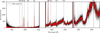 |
Fig. B.1 Primary spectra for all epochs, normalized to 1 around Hα (in black), and mean spectrum (in red). There are no apparent discrepancies between the spectral slopes of the various epochs. |
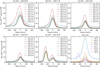 |
Fig. B.2 Balmer lines of the host binary of Delorme 1 (AB)b. |
Appendix C Companion individual lines
The lines for each individual exposure can be found in Figs. C.1, C.2, C.3 and C.4 for Hα, Hβ, Hγ and Hδ, respectively. The lines fluxes for each line can be found in Table C.1. The integrated flux of each wing and core component can be found in Table C.2.
Integrated lines fluxes of Delorme 1 (AB)b, where cgs stands for erg/s/cm2 in the case of lines, and erg/s/cm2/Å for the UV excess mean flux, computed on the 3350−3600 Å range.
Integrated fluxes for each wing and core component of the Hα, Hβ, Hγ and Hδ lines of Delorme 1 (AB)b, where cgs stands for erg/s/cm2.
 |
Fig. C.1 Hα line for all individual epochs. Times are UT in hours:minutes:seconds format. In the last panel, the shaded region represents the standard deviation among all epochs. λ0=6564.66464 Å (vacuum). |
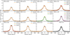 |
Fig. C.2 Hβ line for all individual epochs. Times are UT in hours:minutes:seconds format. In the last panel, the shaded region represents the standard deviation among all epochs. λ0 = 4862.71 Å (vacuum). |
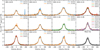 |
Fig. C.3 Hγ line for all individual epochs. Times are UT in hours:minutes:seconds format. In the last panel, the shaded region represents the standard deviation among all epochs. λ0 = 4341.692 Å (vacuum). |
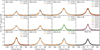 |
Fig. C.4 Hδ line for all individual epochs. Times are UT in hours:minutes:seconds format. In the last panel, the shaded region represents the standard deviation among all epochs. λ0=4102.86503488 Å (vacuum). |
Appendix D Lines decomposition
The lines decomposition for each individual line is shown in Figs. D.2, D.3, D.5 and D.4 for Hα, Hβ, Hγ and Hδ, respectively.
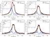 |
Fig. D.1 wing and core component decomposition of the Hα, Hβ, Hγ, and Hδ lines for epoch 2022-10-15-06:30:49 (black). The blue-green shaded lines correspond to successive iterations of the decomposition. The solid blue and green lines correspond to the final iteration. The red line represents the total model at the last iteration. The inset corresponds to the scaling factor of each of the wing and core components, depending on the epoch. The points are color-coded for each epoch, as in Fig. 4. The crosses correspond to the outburst epochs. |
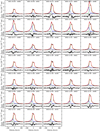 |
Fig. D.2 Two-component fits of Hα, for all epochs, at the last iteration. Each subpanel is divided into the fit and the corresponding residuals. |
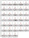 |
Fig. D.3 Two-component fits of Hβ, for all epochs, at the last iteration. Each subpanel is divided into the fit and the corresponding residuals. |
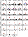 |
Fig. D.4 Two-component fits of Hγ, for all epochs, at the last iteration. Each subpanel is divided into the fit and the corresponding residuals. |
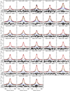 |
Fig. D.5 Two-component fits of Hδ, for all epochs, at the last iteration. Each subpanel is divided into the fit and the corresponding residuals. |
Appendix E Nonnegative matrix factorization
Our decomposition of the H i emission line profiles with the L-BFGS-B approach is in fact similar to a dimension reduction problem encountered in signal processing. We therefore considered using principal component analysis to check whether we could retrieve similar components as with the L-BFGS-B approach, which may still be sensitive to local minima in the parameter space of the fit. But one must impose the principal components to be additive. We therefore considered nonnegative matrix factorization (NMF) using the sklearn implementation of the method (Lee & Seung 1999) with Non-negative Double Singular Value Decomposition (NNDSVD) initialization (Boutsidis & Gallopoulos 2008).
The NMF method assumes that all data have positive values. For that purpose, we added a constant value to bring any negative value in our profile to zero before running the NMF decomposition. A comparison between the decomposition presented in this work, and the NMF results (for Hα) is shown in Fig. E.1.
The decomposition with two components broadly confirm the one achieved with the L-BFGS-B. The wing component is well reproduced for Hα to Hβ. We only notice for Hα a slight change in the blue wing (more extended in the case of the NMF) and a change of slope at the peak of the core component. We also find the second component (wings) to be systematically fainter at Hα than with the L-BFGS-B decomposition at all epochs, and even null in the case of the faintest epochs.
The NMF allows us to more easily explore the possibility of a larger number of components. We find that Hα can require an additional component but its shape is nearly identical to the shape of the profile at the brightest epochs. However, the two main components still conserves qualitatively the same shape. Conversely, we find the results (even with two components) to be much more sensitive to the initialization method of the algorithm. It should be noted that the NMF decomposition requires the addition of a constant “additive” component, which likely biases the fine structure of the derived components.
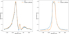 |
Fig. E.1 Comparison of the decomposition presented in this work (based on the L-BFGS-B algorithm) and the corresponding NMF decomposition. |
Appendix F Modeling results
F.1 Lines modeling
This section presents the  maps of the lines modeling (Sect. 5). Figures F.1 and F.2 show the
  maps over the Magnetospheric Accretion models grid (Thanathibodee et al. 2019a), for Hα and Hβ, respectively, in both the core-fitting and the full-line fitting. Figures F.3 and F.4 show a sketch of the best fits for Hα and Hβ, in both the core-fitting and the full-line fitting cases.
F.2 UV modeling
Figure F.5 shows the comparison between the total line flux of each component (wing and core) and the accretion luminosity derived from the UV excess slab-modeling, allowing us to compare to relations from Alcalá et al. (2017).
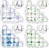 |
Fig. F.1
|


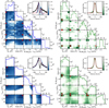 |
Fig. F.2 Same as Figure F.1, but for Hβ. |
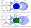 |
Fig. F.3 Sketch of the best-fit model for the core of both the wing and the core components of Hα (top) and Hβ (bottom). The blue and green lines in the top right of the image correspond to the line of sight intercepting the shock. The different inclinations for the blue and green lines are due to the two local minima in the grid (see Figs. F.1 and F.2). The planet in the center and its “apparent shell” of a different color represent the size of the planet in the wing (blue) and core (green) component modeling. Left insets: Data for the wing and core (blue and green) components and the best fit (black line), along with the fitting limits (dashed red lines). |
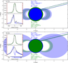 |
Fig. F.4 Same as Fig. F.3, but for the full fitting range. Sketch of the best-fit model for the full range of both the wing and the core components of Hα (top) and Hβ (bottom). The blue and green lines in the top right of the image corresponds to the line of sight intercepting the shock. The planet in the center and its “apparent shell” of a different color represent the size of the planet in the wing (blue) and core (green) component modeling. Left insets: Data for the wing and core (blue and green) components and the best-fit (black line), along with the fitting limits (dashed red lines). |
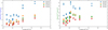 |
Fig. F.5 Comparison between the total line flux of each component (wing and core) and the accretion luminosity derived from the UV excess slab-modeling (see Sect. 5.3). |
Appendix G Looking for remaining uncertainties on the flux calibration of Delorme 1 (AB)b
We show in Figure G.1 a comparison of the spectrum of Delorme 1 AB to the published photometry at optical and nearUV wavelengths converted to flux densities with the VOSA1 tool (Bayo et al. 2008). We used the corresponding filter transmissions available on the Spanish Virtual Observatory2 to compute synthetic fluxes from the UVES spectrum. The transmission curves of each filter is shown at the bottom in the figure. The blind zones corresponding to the detector gaps and split between the red and BLUE arms were replaced by linear interpolation.
The difference between the synthetic and observed flux densities were used to compute renormalization factors for the three separate spectra collected by the three detectors of UVES (1.70 ± 0.12 for the BLUE arm based on the APASS B photometry, 0.86 ± 0.02 for the BLUE arm based on the SkyMapper v-band photometry, 1.27 ± 0.05 for the ship operating at short wavelengths in the RED arm based on APASS V, and 1.17 ± 0.02 for the large wavelengths of the RED arm based on SDSS r). We overlay the MUSE spectrum of the binary star extracted from the flux-calibrated data cubes over a circular aperture of 30 pixels (0.75′′) (calibration achieved with the ESO MUSE pipeline; see Eriksson et al. 2020). The UVES and MUSE spectra have similar spectral features, but the MUSE spectrum is redder and over-luminous compared to UVES and to the reference photometry.
We cannot exclude however that Delorme 1 AB has a more variable photometry in the near-UV than in the V band on long timescales because it is an active star and this region contains many bright emission lines. This is in fact suggested by the different factors found for the SkyMapper and APASS photometry.
We show in Figure G.2 the comparison of the UVES spectrum to the X-SHOOTER spectrum of the young M5 class III star SO641 from Manara et al. (2013b). The comparison reveal close spectral features, and a good correspondence of the spectral slopes longward of 430 nm, confirming the M5 spectroscopic spectral type of Delorme 1 AB quoted in Kraus et al. (2014) and that the scalings quoted above may be due to variability. The X-SHOOTER spectrum of the class III M5.5 star S999 from Manara et al. (2013b) also provide a good fit to the data, although the overtone of TiO at 540 nm is not as deep in the template and our BLUE arm data appears over-luminous by 48% shortward of 450 nm.
We conclude that these comparisons rather confirm the reliability of the flux calibration of our data. We have therefore decided not to correct them from any extra scaling parameters to avoid introducing any additional bias.
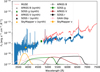 |
Fig. G.1 UVES spectrum of Delorme 1 AB (blue) compared to the available photometry of the binary at optical and near-UV wavelengths. |
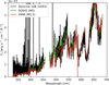 |
Fig. G.2 Comparison of the UVES spectrum of Delorme 1 AB to the VLT/X-SHOOTER spectra of class III dwarfs, renormalized to the Delorme 1 AB mean flux from 500 to 650 nm. |
All Tables
Parameter ranges for the magnetospheric accretion models (Thanathibodee et al. 2019a) and best-fit results.
Integrated lines fluxes of Delorme 1 (AB)b, where cgs stands for erg/s/cm2 in the case of lines, and erg/s/cm2/Å for the UV excess mean flux, computed on the 3350−3600 Å range.
Integrated fluxes for each wing and core component of the Hα, Hβ, Hγ and Hδ lines of Delorme 1 (AB)b, where cgs stands for erg/s/cm2.
All Figures
|
Fig. 1 Illustration of the extraction process for one of the exposures in the RED arm. Left: 2D reconstructed slit, before (top) and after (bottom) subtraction of the PSF models for both the primary and the companion. Right: illustration of the extraction process at a single wavelength bin within Hα. The blue- and green-shaded regions are the various Gaussian components used in the PSF fitting process for the primary and companion, respectively (three Gaussian components here for the RED arm). Bottom panels: modeling residuals. |
| In the text | |
|
Fig. 2 Illustration of the residual contamination correction for the exposure 2022-11-05 UT 01:22:25. This corresponds to the case with the highest contamination. Top panel: residual contamination factor (black) smoothed with a 10 px wide-moving Gaussian box (red) and its associated error bars (black-shaded region). Middle panel: companion spectrum as the output of the extraction process (black) with the contamination contribution (red) and the contamination-corrected companion spectrum (green). All black-shaded regions were excluded from the fit; they correspond to emission lines and detector edges. Third row: contamination contribution within emission lines (same colors). The contamination removal process is able to remove most of the residual primary flux in the companion spectrum, which accounts for ∼10% of the lines flux depending on the exposure. |
| In the text | |
|
Fig. 3 Final spectra over the full spectral range. All Delorme 1 (AB)b spectra, overlaid in black, with the mean spectrum in red. All spectra were smoothed to R = 5000 for clarity. The UV excess of Delorme 1 (AB)b is clearly visible below ∼3700 Å, as well as the generally flat continuum shape. The line marked as an artifact is due to a bad-pixel row on the detector. |
| In the text | |
|
Fig. 4 Balmer lines of Delorme 1 (AB)b. Each panel shows the mean line of each observing epoch (11 epochs), from Hα to Hϵ. The last panel shows the mean line (over all epochs) for each transition order up to Hθ/H10. All lines were plotted after subtracting the local continuum baseline, averaged between (−750;−400) and (+400;+750) km/s. The lines show great profile and amplitude variability across epochs. |
| In the text | |
|
Fig. 5 Comparison of the mean Hα line profile of Delorme 1 (AB)b to that of two young substellar objects with disks (left: CFHT BD Tau 4, center: ChaHa-1) and of a Class III 15 MJup brown dwarf (right: KPNO Tau 4). We scaled (in red) the profile of Ca Ha 1 to the free-fall velocities expected for Delorme 1 (AB)b. The profiles are similar to that of CFHS BD Tau 4 and ChaHa-1, but not to that of KPNO Tau 4. |
| In the text | |
|
Fig. 6 Autocorrelations of the lines Hα, Hβ, and Hγ. The color indicates the value of the Pearson correlation coefficient. The lines were smoothed to R ∼ 40 000 to remove some of the noisy features. The lack of correlation between the wings and the core suggests that the lines may be made of two subcomponents. Overplotted in blue and green are the two subcomponent decompositions obtained in Section 4.5, explaining the features of the autocorrelation. The correlation diagrams for the higher order lines have the same overall shape as Hβ and Hγ. |
| In the text | |
|
Fig. 7 Illustration of the decomposition for three different exposures for Hα (first row) and Hβ (second row). The two components are shown in blue and green, the total model in red, and the corresponding data in black. The decompositions for all exposures are shown in Figs. C.1, C.2, C.3 and C.4 for Hα, Hβ, Hγ, and Hδ, respectively. This decomposition provides a great fit to all exposures despite the strong constraint of a constant profile. |
| In the text | |
|
Fig. 8 Correlations between the wing and core components over multiple lines (Hα to Hδ), the mean continuum level (cont) around Hα (in 10−17 erg/s/cm2/Å), and the mean level of the UV excess (in 10−17 erg/s/cm2/Å). The Pearson correlation coefficient is given as text in each panel. The dashed black line is the y=x line. The blue and green lines and shaded regions are the best affine fit. The color coding of the data points is the same as in Fig. 4. The x and y units are normalized scaling factors of each component. The epoch on October 13, 2022, (orange) was excluded from the analysis because it is so far off the correlation in the core Hα component. The wing and core components are strongly correlated. However, only the wing components have a strong correlation with the UV excess, which could be due to accretion. The wing component and the UV excess are both strongly correlated with the continuum level around Hα, which suggests that the apparent continuum is veiled by the extension of the apparent continuum. |
| In the text | |
|
Fig. 9 Variability diagrams of Hα (left) and Hβ (right) relative flux for all pairs, as a function of the timescale, following the same method as Demars et al. (2023). We show the variability amplitude of the wing (blue) and core (green) components and of the total profile (dark red). The error bars represent the spread of the variability within a given timescale bin, weighted by the significance of the measurement: the σ-distance between the two lines corresponding to the measurement. Higher order lines have variability diagrams similar to that of Hβ, with slightly increased variability amplitude at hours timescales (see Fig. 10). The full-line variability amplitude is driven by that of the core component, because it contains most of the line flux, whereas the wing component is quite faint in comparison. |
| In the text | |
|
Fig. 10 Variability of the Balmer lines at the hourly timescale. The color of the points represents the component (blue for wings and green for core) or the full line (brown). Error bars represent the spread of the variability (weighted by significance), i.e., the brown crosses in Fig. 9. The shaded region corresponds to lines where the detection is compatible with contamination from the host binary. The hourly timescale variability seems to increase with the order of the transition. The wing component has a much higher variability amplitude than the green component. |
| In the text | |
|
Fig. 11 Line ratios decrements. For each line, the line ratio is computed with respect to Hβ (H4). In black, the line ratios of the full-lines in this study are shown. Colored lines correspond to the four decrement types identified in Antoniucci et al. (2017) (see their Fig. 3). Blue and green lines represent the subcomponents (wing and core) obtained in Sect. 4.5. The shaded region corresponds to the lines, which may result from contamination from the host binary (as in Fig. 10). The full-line decrement (black) is broadly compatible with Type 2 case (optically thin emission and low accretion rate). The wing component is not clearly compatible with any decrement type. However, the core component is compatible with the Type 3 sources, which are not easily reproduced by emission line models (Antoniucci et al. 2017). |
| In the text | |
|
Fig. 12 Modeling results for the magnetospheric accretion models (Thanathibodee et al. 2019a). Left: results for the wing subcomponent. Right: results for the core subcomponent. First row: Hα. Second row: Hβ. Each left subpanel corresponds to the fit performed on the [−50; +50] km/s range, while the right subpanels correspond to the fit on the full the line width ([−250; +250] km/s). The red line is the best model, while the colored lines represent a sample of the lowest |
| In the text | |
|
Fig. 13 Modeling results for the shock models (Aoyama et al. 2018), with the flux scaling corresponding to epoch 2022-10-14 – 06:52:50). On each row, the left panel shows the core component for that line (black line), a sample of the best fits (green lines) and the best fit (red line). Right panel: corresponding |
| In the text | |
|
Fig. 14 Evolution of the accretion rate inferred from shock modeling of the core component, depending on the line. The accretion rate is computed as Ṁ=S n0v0μ. The right axis shows the corresponding Lacc = GṀMp/Rp, with Mp = 13 MJup and Rp = 1.5 RJup. The accretion rates inferred from different lines are systematically ordered, which may point to a bias from deriving accretion rates from a single line. |
| In the text | |
|
Fig. 15 Correlations between the accretion luminosity (Lacc) obtained from the UV excess fitting (slab-modeling) and the wing (left) and core (right) components fluxes (Alcalá et al. 2017). The black line shows the Y = X curve. The average accretion luminosity derived from the wing components of various lines is correlated with the accretion luminosity derived from that of slab-modeling (Sect. 5.3), while the accretion luminosity derived from the core component is well above it. |
| In the text | |
|
Fig. 16 Best-fit results to the UV excess and general continuum level using the slab models. The colored lines represent the individual mean epochs. The best fit components are shown for the UV excess (black, slab), photospheric template (light blue, class III), and total model (red). The data were smoothed to R ∼ 250; points below 20% the median level are masked; and a dashed line at 10−18 erg/s/cm2/Å is plotted at each epoch. All spectra are given in erg/s/cm2/Å units. The modeling provides a good fit to the UV excess and shows that almost all epochs have their continuum dominated by the shock-component extending to higher wavelengths. This is particularly evident in outburst epochs (2022-10-14/15). |
| In the text | |
|
Fig. B.1 Primary spectra for all epochs, normalized to 1 around Hα (in black), and mean spectrum (in red). There are no apparent discrepancies between the spectral slopes of the various epochs. |
| In the text | |
|
Fig. B.2 Balmer lines of the host binary of Delorme 1 (AB)b. |
| In the text | |
|
Fig. C.1 Hα line for all individual epochs. Times are UT in hours:minutes:seconds format. In the last panel, the shaded region represents the standard deviation among all epochs. λ0=6564.66464 Å (vacuum). |
| In the text | |
|
Fig. C.2 Hβ line for all individual epochs. Times are UT in hours:minutes:seconds format. In the last panel, the shaded region represents the standard deviation among all epochs. λ0 = 4862.71 Å (vacuum). |
| In the text | |
|
Fig. C.3 Hγ line for all individual epochs. Times are UT in hours:minutes:seconds format. In the last panel, the shaded region represents the standard deviation among all epochs. λ0 = 4341.692 Å (vacuum). |
| In the text | |
|
Fig. C.4 Hδ line for all individual epochs. Times are UT in hours:minutes:seconds format. In the last panel, the shaded region represents the standard deviation among all epochs. λ0=4102.86503488 Å (vacuum). |
| In the text | |
|
Fig. D.1 wing and core component decomposition of the Hα, Hβ, Hγ, and Hδ lines for epoch 2022-10-15-06:30:49 (black). The blue-green shaded lines correspond to successive iterations of the decomposition. The solid blue and green lines correspond to the final iteration. The red line represents the total model at the last iteration. The inset corresponds to the scaling factor of each of the wing and core components, depending on the epoch. The points are color-coded for each epoch, as in Fig. 4. The crosses correspond to the outburst epochs. |
| In the text | |
|
Fig. D.2 Two-component fits of Hα, for all epochs, at the last iteration. Each subpanel is divided into the fit and the corresponding residuals. |
| In the text | |
|
Fig. D.3 Two-component fits of Hβ, for all epochs, at the last iteration. Each subpanel is divided into the fit and the corresponding residuals. |
| In the text | |
|
Fig. D.4 Two-component fits of Hγ, for all epochs, at the last iteration. Each subpanel is divided into the fit and the corresponding residuals. |
| In the text | |
|
Fig. D.5 Two-component fits of Hδ, for all epochs, at the last iteration. Each subpanel is divided into the fit and the corresponding residuals. |
| In the text | |
|
Fig. E.1 Comparison of the decomposition presented in this work (based on the L-BFGS-B algorithm) and the corresponding NMF decomposition. |
| In the text | |
|
Fig. F.1
|
| In the text | |
|
Fig. F.2 Same as Figure F.1, but for Hβ. |
| In the text | |
|
Fig. F.3 Sketch of the best-fit model for the core of both the wing and the core components of Hα (top) and Hβ (bottom). The blue and green lines in the top right of the image correspond to the line of sight intercepting the shock. The different inclinations for the blue and green lines are due to the two local minima in the grid (see Figs. F.1 and F.2). The planet in the center and its “apparent shell” of a different color represent the size of the planet in the wing (blue) and core (green) component modeling. Left insets: Data for the wing and core (blue and green) components and the best fit (black line), along with the fitting limits (dashed red lines). |
| In the text | |
|
Fig. F.4 Same as Fig. F.3, but for the full fitting range. Sketch of the best-fit model for the full range of both the wing and the core components of Hα (top) and Hβ (bottom). The blue and green lines in the top right of the image corresponds to the line of sight intercepting the shock. The planet in the center and its “apparent shell” of a different color represent the size of the planet in the wing (blue) and core (green) component modeling. Left insets: Data for the wing and core (blue and green) components and the best-fit (black line), along with the fitting limits (dashed red lines). |
| In the text | |
|
Fig. F.5 Comparison between the total line flux of each component (wing and core) and the accretion luminosity derived from the UV excess slab-modeling (see Sect. 5.3). |
| In the text | |
|
Fig. G.1 UVES spectrum of Delorme 1 AB (blue) compared to the available photometry of the binary at optical and near-UV wavelengths. |
| In the text | |
|
Fig. G.2 Comparison of the UVES spectrum of Delorme 1 AB to the VLT/X-SHOOTER spectra of class III dwarfs, renormalized to the Delorme 1 AB mean flux from 500 to 650 nm. |
| In the text | |
Current usage metrics show cumulative count of Article Views (full-text article views including HTML views, PDF and ePub downloads, according to the available data) and Abstracts Views on Vision4Press platform.
Data correspond to usage on the plateform after 2015. The current usage metrics is available 48-96 hours after online publication and is updated daily on week days.
Initial download of the metrics may take a while.