| Issue |
A&A
Volume 707, March 2026
|
|
|---|---|---|
| Article Number | A232 | |
| Number of page(s) | 27 | |
| Section | Extragalactic astronomy | |
| DOI | https://doi.org/10.1051/0004-6361/202557329 | |
| Published online | 17 March 2026 | |
Euclid preparation
LXXXII. Predicting star-forming galaxy scaling relations with the spectral stacking code SpectraPyle
1
Dipartimento di Fisica e Astronomia “Augusto Righi” – Alma Mater Studiorum Università di Bologna, via Piero Gobetti 93/2, 40129 Bologna, Italy
2
INAF-Osservatorio di Astrofisica e Scienza dello Spazio di Bologna, Via Piero Gobetti 93/3, 40129 Bologna, Italy
3
INAF-IASF Milano, Via Alfonso Corti 12, 20133 Milano, Italy
4
Dipartimento di Fisica e Astronomia “G. Galilei”, Università di Padova, Via Marzolo 8, 35131 Padova, Italy
5
INAF-Osservatorio Astronomico di Padova, Via dell’Osservatorio 5, 35122 Padova, Italy
6
Department of Physics, Oxford University, Keble Road Oxford, OX1 3RH, UK
7
Aix-Marseille Université, CNRS, CNES, LAM, Marseille, France
8
Dipartimento di Fisica e Astronomia, Università di Bologna, Via Gobetti 93/2, 40129 Bologna, Italy
9
ESAC/ESA, Camino Bajo del Castillo, s/n., Urb. Villafranca del Castillo, 28692 Villanueva de la Cañada, Madrid, Spain
10
INAF-Osservatorio Astronomico di Brera, Via Brera 28, 20122 Milano, Italy
11
Minnesota Institute for Astrophysics, University of Minnesota, 116 Church St SE Minneapolis, MN 55455, USA
12
Université Paris-Saclay, Université Paris Cité, CEA, CNRS, AIM, 91191 Gif-sur-Yvette, France
13
INAF-Osservatorio Astronomico di Capodimonte, Via Moiariello 16, 80131 Napoli, Italy
14
Universitäts-Sternwarte München, Fakultät für Physik, Ludwig-Maximilians-Universität München, Scheinerstr. 1, 81679 München, Germany
15
INAF-Istituto di Astrofisica e Planetologia Spaziali, via del Fosso del Cavaliere 100, 00100 Roma, Italy
16
Instituto de Astrofísica de Canarias, E-38205 La Laguna; Universidad de La Laguna, Dpto. Astrofísica, E-38206 La Laguna, Tenerife, Spain
17
Institute of Space Sciences (ICE, CSIC), Campus UAB, Carrer de Can Magrans, s/n, 08193 Barcelona, Spain
18
INAF-Osservatorio Astronomico di Trieste, Via G. B. Tiepolo 11, 34143 Trieste, Italy
19
School of Physical Sciences, The Open University, Milton Keynes, MK7 6AA, UK
20
INAF-Osservatorio Astrofisico di Arcetri, Largo E. Fermi 5, 50125 Firenze, Italy
21
Dipartimento di Fisica e Astronomia, Università di Firenze, via G. Sansone 1, 50019 Sesto Fiorentino, Firenze, Italy
22
Institute of Physics, Laboratory for Galaxy Evolution, Ecole Polytechnique Fédérale de Lausanne, Observatoire de Sauverny, CH-1290 Versoix, Switzerland
23
Dipartimento di Fisica e Astronomia “Augusto Righi” – Alma Mater Studiorum Università di Bologna, Viale Berti Pichat 6/2, 40127 Bologna, Italy
24
SRON Netherlands Institute for Space Research, Landleven 12, 9747 AD Groningen, The Netherlands
25
Kapteyn Astronomical Institute, University of Groningen, PO Box 800, 9700 AV Groningen, The Netherlands
26
Univ. Lille, CNRS, Centrale Lille, UMR 9189 CRIStAL, 59000 Lille, France
27
Université Paris-Saclay, CNRS, Institut d’astrophysique spatiale, 91405 Orsay, France
28
Instituto de Astrofísica de Canarias, E-38205 La Laguna, Tenerife, Spain
29
Université PSL, Observatoire de Paris, Sorbonne Université, CNRS, LERMA, 75014 Paris, France
30
Université Paris-Cité, 5 Rue Thomas Mann, 75013 Paris, France
31
School of Mathematics and Physics, University of Surrey, Guildford, Surrey, GU2 7XH, UK
32
IFPU, Institute for Fundamental Physics of the Universe, via Beirut 2, 34151 Trieste, Italy
33
INFN, Sezione di Trieste, Via Valerio 2, 34127 Trieste TS, Italy
34
SISSA, International School for Advanced Studies, Via Bonomea 265, 34136 Trieste TS, Italy
35
INFN-Sezione di Bologna, Viale Berti Pichat 6/2, 40127 Bologna, Italy
36
Dipartimento di Fisica, Università di Genova, Via Dodecaneso 33, 16146 Genova, Italy
37
INFN-Sezione di Genova, Via Dodecaneso 33, 16146 Genova, Italy
38
Department of Physics “E. Pancini”, University Federico II, Via Cinthia 6, 80126 Napoli, Italy
39
Instituto de Astrofísica e Ciências do Espaço, Universidade do Porto, CAUP, Rua das Estrelas, PT4150-762 Porto, Portugal
40
Faculdade de Ciências da Universidade do Porto, Rua do Campo de Alegre, 4150-007 Porto, Portugal
41
European Southern Observatory, Karl-Schwarzschild-Str. 2, 85748 Garching, Germany
42
Dipartimento di Fisica, Università degli Studi di Torino, Via P. Giuria 1, 10125 Torino, Italy
43
INFN-Sezione di Torino, Via P. Giuria 1, 10125 Torino, Italy
44
INAF-Osservatorio Astrofisico di Torino, Via Osservatorio 20, 10025 Pino Torinese (TO), Italy
45
European Space Agency/ESTEC, Keplerlaan 1, 2201 AZ Noordwijk, The Netherlands
46
Institute Lorentz, Leiden University, Niels Bohrweg 2, 2333 CA Leiden, The Netherlands
47
Leiden Observatory, Leiden University, Einsteinweg 55, 2333 CC Leiden, The Netherlands
48
Centro de Investigaciones Energéticas, Medioambientales y Tecnológicas (CIEMAT), Avenida Complutense 40, 28040 Madrid Spain
49
Port d’Informació Científica, Campus UAB, C. Albareda s/n, 08193 Bellaterra (Barcelona), Spain
50
Institute for Theoretical Particle Physics and Cosmology (TTK), RWTH Aachen University, 52056 Aachen, Germany
51
INAF-Osservatorio Astronomico di Roma, Via Frascati 33, 00078 Monteporzio Catone, Italy
52
INFN section of Naples, Via Cinthia 6, 80126 Napoli, Italy
53
Institute for Astronomy, University of Hawaii, 2680 Woodlawn Drive Honolulu, HI, 96822, USA
54
Institute for Astronomy, University of Edinburgh, Royal Observatory, Blackford Hill Edinburgh, EH9 3HJ, UK
55
Jodrell Bank Centre for Astrophysics, Department of Physics and Astronomy, University of Manchester, Oxford Road Manchester, M13 9PL, UK
56
European Space Agency/ESRIN, Largo Galileo Galilei 1, 00044 Frascati, Roma, Italy
57
Université Claude Bernard Lyon 1, CNRS/IN2P3, IP2I Lyon, UMR 5822, Villeurbanne, F-69100, France
58
Institut de Ciències del Cosmos (ICCUB), Universitat de Barcelona (IEEC-UB), Martí i Franquès 1, 08028 Barcelona, Spain
59
Institució Catalana de Recerca i Estudis Avançats (ICREA), Passeig de Lluís Companys 23, 08010 Barcelona, Spain
60
UCB Lyon 1, CNRS/IN2P3, IUF, IP2I Lyon, 4 rue Enrico Fermi, 69622 Villeurbanne, France
61
Departamento de Física, Faculdade de Ciências, Universidade de Lisboa, Edifício C8, Campo Grande, PT1749-016 Lisboa, Portugal
62
Instituto de Astrofísica e Ciências do Espaço, Faculdade de Ciências, Universidade de Lisboa, Campo Grande, 1749-016 Lisboa, Portugal
63
Department of Astronomy, University of Geneva, ch. d’Ecogia 16, 1290 Versoix, Switzerland
64
INFN-Padova, Via Marzolo 8, 35131 Padova, Italy
65
Aix-Marseille Université, CNRS/IN2P3, CPPM, Marseille, France
66
Space Science Data Center, Italian Space Agency, via del Politecnico snc, 00133 Roma, Italy
67
INFN-Bologna, Via Irnerio 46, 40126 Bologna, Italy
68
Max Planck Institute for Extraterrestrial Physics, Giessenbachstr. 1, 85748 Garching, Germany
69
Dipartimento di Fisica “Aldo Pontremoli”, Università degli Studi di Milano, Via Celoria 16, 20133 Milano, Italy
70
INFN-Sezione di Milano, Via Celoria 16, 20133 Milano, Italy
71
Institute of Theoretical Astrophysics, University of Oslo, P.O. Box 1029 Blindern, 0315 Oslo, Norway
72
Jet Propulsion Laboratory, California Institute of Technology, 4800 Oak Grove Drive Pasadena, CA, 91109, USA
73
Department of Physics, Lancaster University, Lancaster, LA1 4YB, UK
74
Felix Hormuth Engineering, Goethestr. 17, 69181 Leimen, Germany
75
Technical University of Denmark, Elektrovej 327, 2800 Kgs. Lyngby, Denmark
76
Cosmic Dawn Center (DAWN), Denmark
77
Institut d’Astrophysique de Paris, UMR 7095, CNRS, and Sorbonne Université, 98 bis boulevard Arago, 75014 Paris, France
78
Max-Planck-Institut für Astronomie, Königstuhl 17, 69117 Heidelberg, Germany
79
NASA Goddard Space Flight Center, Greenbelt, MD, 20771, USA
80
Department of Physics and Astronomy, University College London, Gower Street London, WC1E 6BT, UK
81
Department of Physics and Helsinki Institute of Physics, Gustaf Hällströmin katu 2 University of Helsinki, 00014 Helsinki, Finland
82
Université de Genève, Département de Physique Théorique and Centre for Astroparticle Physics, 24 quai Ernest-Ansermet, CH-1211 Genève 4, Switzerland
83
Department of Physics, P.O. Box 64 University of Helsinki, 00014 Helsinki, Finland
84
Helsinki Institute of Physics, Gustaf Hällströmin katu 2 University of Helsinki, 00014 Helsinki, Finland
85
Laboratoire d’etude de l’Univers et des phenomenes eXtremes, Observatoire de Paris, Université PSL, Sorbonne Université, CNRS, 92190 Meudon, France
86
SKAO, Jodrell Bank, Lower Withington, Macclesfield, SK11 9FT, UK
87
Centre de Calcul de l’IN2P3/CNRS, 21 avenue Pierre de Coubertin, 69627 Villeurbanne Cedex, France
88
University of Applied Sciences and Arts of Northwestern Switzerland, School of Computer Science, 5210 Windisch, Switzerland
89
Universität Bonn, Argelander-Institut für Astronomie, Auf dem Hügel 71, 53121 Bonn, Germany
90
INFN-Sezione di Roma, Piazzale Aldo Moro, 2 – c/o Dipartimento di Fisica Edificio G. Marconi, 00185 Roma, Italy
91
Department of Physics, Institute for Computational Cosmology, Durham University, South Road Durham, DH1 3LE, UK
92
Université Paris Cité, CNRS, Astroparticule et Cosmologie, 75013 Paris, France
93
CNRS-UCB International Research Laboratory, Centre Pierre Binétruy, IRL2007, CPB-IN2P3 Berkeley, USA
94
University of Applied Sciences and Arts of Northwestern Switzerland, School of Engineering, 5210 Windisch, Switzerland
95
Institut d’Astrophysique de Paris, 98bis Boulevard Arago, 75014 Paris, France
96
Institute of Physics, Laboratory of Astrophysics, Ecole Polytechnique Fédérale de Lausanne (EPFL), Observatoire de Sauverny, 1290 Versoix, Switzerland
97
Telespazio UK S.L. for European Space Agency (ESA), Camino bajo del Castillo, s/n, Urbanizacion Villafranca del Castillo Villanueva de la Cañada, 28692 Madrid, Spain
98
Institut de Física d’Altes Energies (IFAE), The Barcelona Institute of Science and Technology, Campus UAB, 08193 Bellaterra (Barcelona), Spain
99
DARK, Niels Bohr Institute, University of Copenhagen, Jagtvej 155, 2200 Copenhagen, Denmark
100
Waterloo Centre for Astrophysics, University of Waterloo, Waterloo, Ontario, N2L 3G1, Canada
101
Department of Physics and Astronomy, University of Waterloo, Waterloo, Ontario, N2L 3G1, Canada
102
Perimeter Institute for Theoretical Physics, Waterloo, Ontario, N2L 2Y5, Canada
103
Centre National d’Etudes Spatiales – Centre spatial de Toulouse, 18 avenue Edouard Belin, 31401 Toulouse Cedex 9, France
104
Institute of Space Science, Str. Atomistilor, nr. 409 Măgurele Ilfov, 077125, Romania
105
Consejo Superior de Investigaciones Cientificas, Calle Serrano 117, 28006 Madrid, Spain
106
Universidad de La Laguna, Dpto. Astrofísica, E-38206 La Laguna, Tenerife, Spain
107
Institut für Theoretische Physik, University of Heidelberg, Philosophenweg 16, 69120 Heidelberg, Germany
108
Institut de Recherche en Astrophysique et Planétologie (IRAP), Université de Toulouse, CNRS, UPS, CNES, 14 Av. Edouard Belin, 31400 Toulouse, France
109
Université St Joseph; Faculty of Sciences, Beirut, Lebanon
110
Departamento de Física, FCFM, Universidad de Chile, Blanco Encalada 2008 Santiago, Chile
111
Universität Innsbruck, Institut für Astro- und Teilchenphysik, Technikerstr. 25/8, 6020 Innsbruck, Austria
112
Institut d’Estudis Espacials de Catalunya (IEEC), Edifici RDIT, Campus UPC, 08860 Castelldefels, Barcelona, Spain
113
Satlantis, University Science Park, Sede Bld 48940 Leioa-Bilbao, Spain
114
Infrared Processing and Analysis Center, California Institute of Technology, Pasadena, CA, 91125, USA
115
Instituto de Astrofísica e Ciências do Espaço, Faculdade de Ciências, Universidade de Lisboa, Tapada da Ajuda, 1349-018 Lisboa, Portugal
116
Cosmic Dawn Center (DAWN)
117
Niels Bohr Institute, University of Copenhagen, Jagtvej 128, 2200 Copenhagen, Denmark
118
Universidad Politécnica de Cartagena, Departamento de Electrónica y Tecnología de Computadoras, Plaza del Hospital 1, 30202 Cartagena, Spain
119
Dipartimento di Fisica e Scienze della Terra, Università degli Studi di Ferrara, Via Giuseppe Saragat 1, 44122 Ferrara, Italy
120
Istituto Nazionale di Fisica Nucleare, Sezione di Ferrara, Via Giuseppe Saragat 1, 44122 Ferrara, Italy
121
INAF, Istituto di Radioastronomia, Via Piero Gobetti 101, 40129 Bologna, Italy
122
Université Côte d’Azur, Observatoire de la Côte d’Azur, CNRS, Laboratoire Lagrange, Bd de l’Observatoire, CS 34229, 06304 Nice cedex 4, France
123
Aurora Technology for European Space Agency (ESA), Camino bajo del Castillo, s/n, Urbanizacion Villafranca del Castillo, Villanueva de la Cañada, 28692 Madrid, Spain
124
INAF – Osservatorio Astronomico di Brera, via Emilio Bianchi 46, 23807 Merate, Italy
125
INAF-Osservatorio Astronomico di Brera, Via Brera 28, 20122 Milano, Italy, and INFN-Sezione di Genova, Via Dodecaneso 33, 16146 Genova, Italy
126
ICL, Junia, Université Catholique de Lille, LITL, 59000 Lille, France
127
ICSC – Centro Nazionale di Ricerca in High Performance Computing, Big Data e Quantum Computing, Via Magnanelli 2 Bologna, Italy
128
Instituto de Física Teórica UAM-CSIC, Campus de Cantoblanco, 28049 Madrid, Spain
129
CERCA/ISO, Department of Physics, Case Western Reserve University, 10900 Euclid Avenue Cleveland, OH 44106, USA
130
Technical University of Munich, TUM School of Natural Sciences, Physics Department, James-Franck-Str. 1, 85748 Garching, Germany
131
Max-Planck-Institut für Astrophysik, Karl-Schwarzschild-Str. 1, 85748 Garching, Germany
132
Laboratoire Univers et Théorie, Observatoire de Paris, Université PSL, Université Paris Cité, CNRS, 92190 Meudon, France
133
Departamento de Física Fundamental. Universidad de Salamanca, Plaza de la Merced s/n, 37008 Salamanca, Spain
134
Université de Strasbourg, CNRS, Observatoire astronomique de Strasbourg, UMR 7550, 67000 Strasbourg, France
135
Center for Data-Driven Discovery, Kavli IPMU (WPI), UTIAS, The University of Tokyo, Kashiwa, Chiba 277-8583, Japan
136
Dipartimento di Fisica – Sezione di Astronomia, Università di Trieste, Via Tiepolo 11, 34131 Trieste, Italy
137
California Institute of Technology, 1200 E California Blvd, Pasadena, CA, 91125, USA
138
Department of Physics & Astronomy, University of California Irvine, Irvine, CA, 92697, USA
139
Departamento Física Aplicada, Universidad Politécnica de Cartagena, Campus Muralla del Mar, 30202 Cartagena, Murcia, Spain
140
Instituto de Física de Cantabria, Edificio Juan Jordá, Avenida de los Castros, 39005 Santander, Spain
141
INFN, Sezione di Lecce, Via per Arnesano CP-193, 73100 Lecce, Italy
142
Department of Mathematics and Physics E. De Giorgi, University of Salento, Via per Arnesano CP-I93, 73100 Lecce, Italy
143
INAF-Sezione di Lecce, c/o Dipartimento Matematica e Fisica, Via per Arnesano, 73100 Lecce, Italy
144
CEA Saclay, DFR/IRFU, Service d’Astrophysique, Bat. 709, 91191 Gif-sur-Yvette, France
145
Institute of Cosmology and Gravitation, University of Portsmouth, Portsmouth, PO1 3FX, UK
146
Department of Computer Science, Aalto University, PO Box 15400 Espoo, FI-00 076, Finland
147
Caltech/IPAC, 1200 E. California Blvd. Pasadena, CA, 91125, USA
148
Ruhr University Bochum, Faculty of Physics and Astronomy, Astronomical Institute (AIRUB), German Centre for Cosmological Lensing (GCCL), 44780 Bochum, Germany
149
Department of Physics and Astronomy, Vesilinnantie 5, University of Turku, 20014 Turku, Finland
150
Serco for European Space Agency (ESA), Camino bajo del Castillo, s/n, Urbanizacion Villafranca del Castillo, Villanueva de la Cañada, 28692 Madrid, Spain
151
ARC Centre of Excellence for Dark Matter Particle Physics, Melbourne, Australia
152
Centre for Astrophysics & Supercomputing, Swinburne University of Technology, Hawthorn, Victoria, 3122, Australia
153
Department of Physics and Astronomy, University of the Western Cape, Bellville, Cape Town, 7535, South Africa
154
DAMTP, Centre for Mathematical Sciences, Wilberforce Road Cambridge, CB3 0WA, UK
155
Kavli Institute for Cosmology Cambridge, Madingley Road Cambridge, CB3 0HA, UK
156
Department of Astrophysics, University of Zurich, Winterthurerstrasse 190, 8057 Zurich, Switzerland
157
Department of Physics, Centre for Extragalactic Astronomy, Durham University, South Road Durham, DH1 3LE, UK
158
IRFU, CEA, Université Paris-Saclay, 91191 Gif-sur-Yvette Cedex, France
159
Oskar Klein Centre for Cosmoparticle Physics, Department of Physics, Stockholm University, Stockholm, SE-106 91, Sweden
160
Astrophysics Group, Blackett Laboratory, Imperial College London, London, SW7 2AZ, UK
161
Univ. Grenoble Alpes, CNRS, Grenoble INP, LPSC-IN2P3, 53 Avenue des Martyrs, 38000 Grenoble, France
162
Dipartimento di Fisica, Sapienza Università di Roma, Piazzale Aldo Moro 2, 00185 Roma, Italy
163
Centro de Astrofísica da Universidade do Porto, Rua das Estrelas, 4150-762 Porto, Portugal
164
HE Space for European Space Agency (ESA), Camino bajo del Castillo, s/n, Urbanizacion Villafranca del Castillo Villanueva de la Cañada, 28692 Madrid, Spain
165
INAF – Osservatorio Astronomico d’Abruzzo, Via Maggini, 64100 Teramo, Italy
166
Theoretical astrophysics, Department of Physics and Astronomy, Uppsala University, Box 516, 751 37 Uppsala, Sweden
167
Mathematical Institute, University of Leiden, Einsteinweg 55, 2333 CA Leiden, The Netherlands
168
School of Physics & Astronomy, University of Southampton, Highfield Campus, Southampton, SO17 1BJ, UK
169
Institute of Astronomy, University of Cambridge, Madingley Road Cambridge, CB3 0HA, UK
170
Department of Astrophysical Sciences, Peyton Hall, Princeton University, Princeton, NJ, 08544, USA
171
Space physics and astronomy research unit, University of Oulu, Pentti Kaiteran katu 1, FI-90014 Oulu, Finland
172
Center for Computational Astrophysics, Flatiron Institute, 162 5th Avenue, 10010 New York, NY, USA
★ Corresponding author: This email address is being protected from spambots. You need JavaScript enabled to view it.
Received:
19
September
2025
Accepted:
30
November
2025
Abstract
We introduce SpectraPyle, a versatile spectral stacking pipeline developed for the Euclid mission’s NISP spectroscopic surveys, aimed at extracting faint emission lines and spectral features from large galaxy samples in the Wide and Deep Surveys. Designed for computational efficiency and flexible configuration, SpectraPyle supports the processing of extensive datasets critical to Euclid’s non-cosmological science goals. We validated the pipeline using simulated spectra processed to match Euclid’s expected final data quality. Stacking enables robust recovery of key emission lines, including Hα, Hβ, [O III], and [N II], below individual detection limits. However, the measurement of galaxy properties such as star formation rate, dust attenuation, and gas-phase metallicity are biased at stellar mass below log10(M/ M⊙)∼9 due to the flux-limited nature of Euclid spectroscopic samples, where spectra below the detection threshold lack reliable redshift measurements, preventing effective stacking. The star formation rate–stellar mass relation of the parent sample is recovered reliably only in the deep survey for log10(M/ M⊙)≳10, whereas the metallicity–mass relation is recovered more accurately over a wider mass range. These limitations are caused by the increased fraction of redshift measurement errors at lower masses and fluxes. We examined the impact of residual redshift contaminants that arises from mis-identified emission lines and noise spikes, on stacked spectra. Even after stringent quality selections, low-level contamination (< 6%) has minimal impact on line fluxes due to the systematically weaker emission of contaminants. A percentile-based analysis of stacked spectra provides a sensitive diagnostic for detecting contamination via coherent spurious features at characteristic wavelengths. While our simulations include most instrumental effects, real Euclid data will require a further refinement of contamination mitigation strategies.
Key words: methods: data analysis / techniques: spectroscopic / surveys / galaxies: evolution / galaxies: general / galaxies: star formation
© The Authors 2026
 Open Access article, published by EDP Sciences, under the terms of the Creative Commons Attribution License (https://creativecommons.org/licenses/by/4.0), which permits unrestricted use, distribution, and reproduction in any medium, provided the original work is properly cited.
This article is published in open access under the Subscribe to Open model. This email address is being protected from spambots. You need JavaScript enabled to view it. to support open access publication.
1. Introduction
In many areas of astrophysics, particularly those concerned with the physical properties of distant or faint sources, individual spectra often lack the necessary signal-to-noise ratio (S/N) to detect and characterise key spectral features. This limitation is especially pronounced when studying processes such as star formation, chemical enrichment, or ionisation conditions, which can sometimes rely on the measurement of intrinsically weak emission and absorption lines. Spectral stacking (i.e. combining spectra of different sources) is a widely used method in astrophysics to improve the S/N of low-quality spectra (e.g. Francis et al. 1991). We identified two primary science cases where stacking becomes indispensable: (1) the study of scaling relations and emission line diagnostics, which often target faint lines tracing star formation, active galactic nucleus (AGN) activity, ionised gas conditions, and shocks; and (2) stellar population studies, which require high S/N in the continuum (typically S/N ≳ 30 per Å) to measure features, such as absorption lines and break strengths, that are needed to infer stellar ages, metallicities, alpha-enhancement, and star formation histories (e.g. Choi et al. 2014; Citro et al. 2016).
In this work, we explore how stacking can be effectively applied to Euclid spectroscopy, taking into account the unique properties and challenges of slitless infrared spectra at low resolution. Euclid is an ongoing ESA medium-class mission (Laureijs et al. 2011; Racca et al. 2016), designed to demonstrate the composition and evolution of the Dark Universe, specifically focussing on dark energy and dark matter. The mission employs two primary cosmological probes, namely weak lensing and galaxy clustering, that are studied through high-resolution imaging and low-resolution slitless spectroscopy, provided by a visible imager (VIS, Euclid Collaboration: Cropper et al. 2025), and the Near-Infrared Spectrometer and Photometer (NISP, Euclid Collaboration: Jahnke et al. 2025). The NISP spectrograph (NISP-S) uses two so-called red grisms (RGS), spanning the same RGE passband (1.206–1.892 μm), and one blue grism (BGS) covering the BGE passband (0.926–1.366 μm). Euclid is conducting two major surveys: Euclid Wide Survey (EWS, Euclid Collaboration: Scaramella et al. 2022), which covers about 14 000 deg2, down to a 5σ point-like source depth of 26.2 (24) in IE (YE, JE, HE), and down to a 3.5σ line flux limit of 2 × 10⁻¹⁶ erg s−1 cm−2 for a target source of diameter  (Euclid Collaboration: Le Brun et al. 2026); as well as Euclid Deep Survey (EDS, Euclid Collaboration: Mellier et al. 2025), which will eventually be approximately two magnitudes deeper and with a flux limit of 6 × 10⁻¹⁷ erg s−1 cm−2 over an area of 53 deg2, split in to three fields.
The unparalleled volume of spectro-photometric data, encompassing precise morphological parameters for billions of galaxies and tens of millions of spectroscopic redshifts, will enable the investigation of scaling relations, mass assembly, environmental effects, and AGN co-evolution in samples that include a significant number of star-forming galaxies at z < 2, as well as massive passive at z > 2, and up to extreme redshift (z > 7) sources (Euclid Collaboration: Mellier et al. 2025; Euclid Collaboration: Selwood et al. 2025). However, the vast majority of spectra, especially from the EWS, have a low S/N in the stellar continuum, while a minimum S/N of ∼5 is generally required to robustly detect and measure emission line fluxes (Euclid Collaboration: Gabarra et al. 2023). Consequently, the direct detection of spectral features in individual spectra is generally limited to the brightest galaxies. Furthermore, many diagnostics rely on multiple line detections. For example, Hβ is required for dust correction and SFR estimates, but it is intrinsically fainter than Hα (typically by a factor of > 3, accounting for extinction). Alternatively, [O III]λ4363, used for direct metallicity estimates via electron temperature, is over 100 times fainter than Hα and blended with Hγ at Euclid’s resolution. Detecting such lines requires stacking dozens to thousands of spectra, depending on the target line and the intrinsic S/N of individual observations. For instance, detecting Hβ in galaxies with typical EWS-quality spectra requires stacking at least a dozen spectra; for auroral lines, up to 10 000–40 000 may be needed.
The steps of creating a composite spectrum involve several critical choices, which can have a substantial impact on the final output (e.g. Francis et al. 1991; Vanden Berk et al. 2001), most of which depend on the scientific question under investigation. We created SpectraPyle, a Python code for stacking low S/N spectra, which not only provides the needed flexibility to be adapted for the study of different science cases, but also streamlines the stacking process for such a large dataset, of thousands of galaxy and AGN spectra per square degree, such as that of Euclid.
A critical aspect of leveraging stacked spectra for noncosmological studies is recognising and correcting for the various systematic effects inherent to the Euclid spectroscopic dataset. First and foremost, the spectroscopic redshift sample is inherently biased: it preferentially selects galaxies with bright emission lines, as these are necessary for reliable redshift determination in slitless spectroscopy. This introduces a flux-limited selection that affects all derived statistics, from emission line diagnostics to inferred physical properties. In addition, slitless spectroscopy is prone to contamination and redshift mis-identifications (interlopers), particularly in crowded fields or at specific redshift ranges where line confusion is common. These issues can skew the final stacked spectra, both by introducing fake features due to noise and contamination, as well as by enhancing certain spectral lines through selection effects. As such, even robust stacking techniques must be applied with caution and an understanding of the biases they may amplify.
This paper explores such issues using Euclid-like mock observations and focussing on the use of stacking techniques to enhance the S/N. We examine how redshift measurement errors, the presence of interlopers (i.e. galaxies assigned incorrect redshifts), and the trade-off between sample completeness (success rate) and contamination affect the recovered spectroscopic sample. In particular, we show how these effects propagate into stacked spectra and influence the measurement of emission line fluxes, the construction of diagnostic line ratios, and ultimately the recovery of galaxy scaling relations such as mass–metallicity trends. We also highlight the presence of biases introduced by sample selection. While we explore these effects within a specific simulation and using a particular analysis pipeline, the findings have general implications for the interpretation of Euclid spectroscopic data. Our goal is to identify and quantify systematic effects that will be present, to varying degrees, in any real Euclid spectroscopic analysis.
The structure of this paper is as follows. In Sect. 2, we introduce the Euclid spectroscopic surveys, whilst in Sect. 3 we describe the SpectraPyle code and its functionalities. Section 4 presents the simulation and the mock Euclid spectra and redshift determination. In Sect. 5 we characterise redshift contamination from various sources and we discuss the impact of redshift contaminants on the stacked spectra. Section 6 defines the success rate and contamination rate of the sample and we examine the biases introduced by flux-limited selection, especially in the context of recovering scaling relations and physical parameters from stacked spectra. In Sect. 7, we analyse some of the aforementioned key scaling relations with Euclid stacked spectra. Finally, in Sect. 8, we summarise our main findings. Throughout this paper, we adopt a flat ΛCDM cosmology with Ωm = 0.3, ΩΛ = 0.7, and H0 = 70 km s−1 Mpc−1. We assume a Chabrier (2003) initial mass function (IMF). All magnitudes are in the AB system.
2. The Euclid spectroscopic surveys
In the EWS, spectra are obtained in the RGS alone, with a wavelength sampling of 1.37 nm pixel−1 and a resolving power R ≃ 500 (Euclid Collaboration: Copin et al. 2026; Euclid Collaboration: Le Brun et al. 2026). The spectroscopic set-up in the EWS is optimised for the detection of about 2000–4800 Hα emitters deg−2 within the redshift range z ∈ [0.84, 1.88] (Pozzetti et al. 2016), for the galaxy clustering probe, but it enables the detection and measurement of other redshifted optical and NIR emission lines that trace the evolution of physical processes in galaxies over the last 8–10 Gyr. More details about the EWS observing strategy can be found in Euclid Collaboration: Scaramella et al. (2022) and Euclid Collaboration: Copin et al. (2026).
For the EDS, NISP-S complement the two RGSs with the BGS, thus extending the lower Hα redshift limit to z = 0.41. The BGS has a constant wavelength sampling of 1.24 nm pixel−1 and an expected resolving power of R ≥ 400. The exposure time ratio between the BGS and RGS will eventually be of 5:3, and the greater sensitivity achieved through repeated observations translates into a 3.5σ flux detection limit for emission lines of 5 × 10⁻¹⁷ erg s−1 cm−2 (Euclid Collaboration: Mellier et al. 2025). Figure 1 shows the redshift extent of prominent emission lines in the EWS and EDS spectra. In Sect. 6, we present examples of science cases related to the various sets of lines detectable in the two surveys.
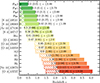 |
Fig. 1. Redshift coverage of prominent emission lines in the EWS and EDS spectra. For each emission line, the full coloured bar represents the redshift range where the line is detectable in the RGS for the EWS, whilst the dashed bar indicates the extended redshift coverage provided by the BGS in the EDS. |
The Euclid pipeline determines redshifts using a template-fitting approach adapted from the Algorithm for Massive Automated Z Evaluation and Determination (AMAZED, Schmitt et al. 2019), and optimised for Euclid slitless spectroscopy (Euclid Collaboration: Le Brun et al. 2026). For the EWS, spectra from the red grism are used, whereas for the EDS the pipeline takes into account also the blue grism to improve redshift accuracy. The fitting procedure produces the probability density function (zPDF), and stores up to five redshift solutions corresponding to the strongest five peaks of the zPDF. For each of the five redshift solutions, the Euclid pipeline provides a probability score (hereafter, zprob), which corresponds to the integrated probability under the zPDF peak (within ±3σ), ranging from 0 (lowest confidence in the redshift estimate) to 1 (highest confidence). In our analysis, where we perform measurements on simulated spectra using the same code, we use only the best-fit solution. In the EWS, a prior is applied in the zPDF calculation to preferentially interpret isolated emission lines in low S/N spectra as the Hα line (Euclid Collaboration: Le Brun et al. 2026). It enhances, in particular, the accuracy of redshift measurements in the range where Hα falls within the red grism, approximately between 0.9 ≲ z ≲ 1.8. This prior could lead to mis-identifications with other bright lines (see Sect. 5.3).
Once the redshift has been determined, the fluxes of the detected emission lines are measured using both direct integration (DI) and Gaussian fitting (GF) methods (Euclid Collaboration: Le Brun et al. 2026). The DI method integrates line flux from the peak position after subtracting the continuum until the flux remains positive, providing flux, S/N, equivalent width (EW), and line centroid position. The GF method models emission lines with multiple Gaussians and a constant continuum. For the lines of the complex Hα + [N II] doublet, which is blended at NISP-S resolution, three Gaussians are used for deconvolution.
3. SpectraPyle: a Euclid-optimised stacking code
In this paper we present SpectraPyle, a Python-based stacking tool designed to combine several spectra from galaxy selected samples to obtain their combined spectra with increased quality. Indeed, when combining n spectra with uncorrelated noise, the resulting S/N typically increases as  , under the assumption that noise is uncorrelated and random. This code will handle the statistical demands and flexibility needed for Euclid-based science. The code is highly modular and provides tools for data preparation that preserve the underlying astrophysical information, enabling an easy adaptation to user needs while remaining compatible with the Euclid data model (Fig. 2). SpectraPyle has been implemented as a key component of the data analysis within the ESA Datalabs (Navarro et al. 2024)1, a collaborative platform that provides access to data processing tools and computational resources for researchers2.
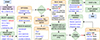 |
Fig. 2. Flowchart of the code SpectraPyle. The letter (d) indicates default options and parameters. |
3.1. Processing the individual spectra
The code processes individual spectra consisting of three mandatory arrays: the wavelength grid (in units of Å), flux values (in units of erg s−1 cm−2 Å−1), and the corresponding errors. Optional arrays may be included, such as quality masks for individual pixels and the number of dithered observations contributing to the co-added flux for each pixel, to exclude low-quality spectral regions from the stacking process. The stacking procedure can be customised through user-defined configuration parameters, such as RGS or BGS selection, flux normalisation, sigma clipping, and bootstrapping. Users can also choose to correct for Galactic extinction on individual spectra before stacking, using the dust_extinction Python package (Gordon 2024).
Individual spectra are shifted to a common reference redshift, which can be set to the minimum, maximum, or median redshift of the sample, a user-defined value, or to the rest frame. If zstack is the target redshift for stacking and zgal is the redshift of an individual galaxy, the wavelength of the i-th pixel (λi) in the galaxy’s spectrum is shifted as
 (1)
(1)
SpectraPyle allows for optional flux normalisation of spectra prior to stacking. The available methods include: ‘regular’ (no normalisation), ‘median’ (scaling each spectrum to its median flux across the full wavelength range), ‘integral’ (scaling to the mean integrated flux), ‘interval’ (scaling to the mean flux within a user-defined wavelength range), and ‘custom’ (user-supplied normalisation factors, e.g. based on photometry, which is particularly useful for faint spectra). If no normalisation is applied (i.e. using the regular option), the code offers two flux-scaling methods when shifting to the common redshift: flux conservation and luminosity conservation, depending on the intended preservation of observed or intrinsic spectral features.
-
The flux conservation approach transforms the flux of the i-th pixel as
 (2)
(2)This transformation preserves integrated flux over a wavelength range (e.g. emission line fluxes), as the (1 + z) terms in Eqs. (1) and (2) cancel out. It is therefore useful when conserving emission line ratios is important. However, it does not preserve the intrinsic luminosity of spectral features, since it does not account for the dimming due to the luminosity distance. As a result, converting stacked fluxes into luminosities is an approximation, whose accuracy depends on the sample’s redshift range and distribution (Appendix A.1).
-
The luminosity conservation method preserves the intrinsic luminosity of spectral features,
 (3)
(3)where DL is the luminosity distance. This method ensures that luminosity-dependent measurements, such as the SFR derived from Hα luminosity, remain correct in the composite spectrum.
In both cases, the spectral continuum of galaxies with zgal < zstack, contributing predominantly to the redder end of the stacked spectrum, will be dimmed, while those with zgal > zstack, contributing more to the bluer end, will be brightened. Therefore, in particular for luminosity conservation, this method should be used only with a narrow distribution of redshifts. Once the spectrum has been shifted, it is resampled onto a common, user-defined wavelength grid using a flux-conserving method, where the spectrum is treated as a step function, with pixel-centred wavelengths and associated flux values. We reconstruct the pixel edges and finely sample each pixel at a fixed resolution (0.01 Å). The flux is then integrated over the new wavelength bins using a simple summation and normalised by the bin widths to yield average flux densities. This approach ensures that the total flux is conserved across the resampling process and avoids interpolation artefacts.
3.2. Combining the spectra
The steps described in the previous subsection are applied to each spectrum individually, resulting in a set of spectra aligned to a common redshift and normalised according to the chosen scheme. A Gaussian sigma-clipping procedure is then applied to the flux distribution at each pixel to identify and discard outliers. By default, pixels with flux values exceeding four standard deviations from the mean are excluded. This threshold can be adjusted by the user as needed. A future upgrade will offer an alternative clipping scheme based on the interquartile range, which may be more suitable for asymmetric or non-Gaussian flux distributions.
The final step is the actual stacking, where the appropriate statistical method applied to combine the spectra depends upon the spectral quantities of interest: users can opt for the arithmetic mean to preserve the broad spectral features, the median to minimise the influence of outliers and preserve relative fluxes of the emission features (i.e. optimal for tracing physical processes traced by emission line ratios), the weighted mean for giving more influence to data points with higher reliability or significance, or the geometric mean for preserving multiplicative relationships within the spectra and to accurately determine the average spectra of objects with fluxes per Å spanning a large dynamic range of several magnitudes (Appendix A.2). By default, SpectraPyle estimates statistical uncertainties on the stacked spectrum using bootstrap resampling with replacement, performing 350 iterations (see Appendix A.3 for details). This number can be adjusted by the user to balance precision and computational cost. This approach provides a robust characterisation of the variability in the stacked signal. Alternatively, users may choose to compute standard errors based on the applied statistical estimator (e.g. mean or median), although this method does not account for sample variance as comprehensively as a bootstrapping approach does.
4. The simulated dataset
4.1. The MAMBO simulation
In this work, we constructed a mock catalogue using Mocks with Abundance Matching in Bologna (MAMBO, Girelli 2021, see also López-López et al. 2024), that we applied to the Millennium Simulation outputs (Springel et al. 2005), tailored to the Planck cosmology (Angulo & White 2010), and specifically to a light-cone derived by Henriques et al. (2015) that covers a redshift range from z = 0 to z = 10. This light-cone includes halos with masses greater than M200 > 1.7 × 10¹⁰ M⊙ over an area of 3.14 deg2, corresponding to approximately 6 independent Euclid pointing of 0.5 deg2 each. In the light-cone, MAMBO assigns a galaxy with stellar mass M* to each dark matter halo, following the stellar-to-halo mass relation (SHMR) by Girelli (2021), calibrated against observed stellar mass functions (SMFs) from surveys such as SDSS (York et al. 2000), COSMOS (Scoville et al. 2007), and CANDELS fields. Galaxies are then classified into two main populations: quiescent and star-forming, using a probabilistic way, following the relative ratio of the blue and red populations in observed SMF (Peng et al. 2010; Ilbert et al. 2013; Girelli et al. 2019). Our MAMBO catalogue does not include AGNs3. The possible presence of a residual population of narrow-line AGNs (noting that broad-line AGNs and QSOs are readily identified and excluded, as demonstrated in recent Quick Data Release 1 analyses; e.g. Euclid Collaboration: Matamoro Zatarain et al. 2026; Fu et al., in preparation) may introduce a modest contribution to the derived scaling relations.
Stellar mass M*, redshift z and galaxy classification are the fundamental parameters from which all other observables are statistically derived using empirical relations, and generated using the Empirical Galaxy Generator (EGG, Schreiber et al. 2017). The resulting catalogues have realistic fluxes and galaxy properties that match current observations from redshifts 0 to 6 by construction, and that are extrapolated up to redshift 10. Controlled random scatter is added to most observables.
In EGG, following the approach of Lang et al. (2014), galaxies are modelled as having two components: a bulge with a Sérsic index n = 4 and a disc with a Sérsic index n = 1. The bulge-to-total ratio (B/T) defines the mass distribution between these components, described by parameters including the projected axis ratio (b/a), half-light radius (R50), and position angle (θ). Position angles for both bulge and disk components are drawn from a uniform distribution. SFRs are assigned based on the empirical main sequence relation between SFR and M* by Schreiber et al. (2015). Physical properties such as size, velocity dispersion, dust attenuation, optical rest-frame colours, and metallicity are also modelled. Then, an appropriate panchromatic spectral energy distribution (SED), for both the disk and bulge components, is assigned to each galaxy. Based on its redshift, M* and quiescent/star-forming classification, each source is randomly placed on the UVJ diagram, where an SED from a pre-built stellar library of Bruzual & Charlot (2003) is pre-assigned to each position. Synthetic photometry is finally generated by integrating the redshifted SED in commonly used broadband filters from UV to submillimeter wavelengths, including the four Euclid VIS and NISP-P bands (i.e. IE, YE, JE, and HE).
The next step thatneeded to create incident spectra, is to add a set of prominent recombination and forbidden emission lines to the SED of the disk component of star-forming galaxies, namely (from redder to bluer): Paβ, Paγ, [S III]λ9531, [S III]λ9069, the [S II]λ6731–[S II]λ6717 doublet (hereafter [S II]), [N II]λ6584–[N II]λ6548 (hereafter [N II]), Hα, [O III]λ5007 (hereafter [O III]), [O III]λ4959, Hβ, [Ne III]λ3869, and the [O II]λ3727 doublet (hereafter [O II]). These spectral features are well-established as highly sensitive tracers of the physical conditions within the ionised gas of galaxies and the nature of the ionising radiation (Osterbrock 1989; Kewley et al. 2019), and their simulated luminosities are generated following empirical relations, starting from their stellar mass and SFR4. Intrinsic emission line luminosities were adjusted to include dust attenuation using the Balmer decrement and the Calzetti et al. (2000) extinction law, while we did not include attenuation due to Galactic extinction to the simulated SEDs. All the lines were initially assumed to have the same velocity dispersion, which was set to the resolution of the Bruzual & Charlot (2003) template (a FWHM of approximately 0.27 nm) to align with the resolution of the stellar component. We finally applied a Gaussian broadening kernel to the composite stellar-emission SED of the disk component and to the stellar SED of the bulge component, using a wavelength-dependent σ(λ) for each pixel that corresponds to the galaxy’s velocity dispersion using the mass-dependent σgas from Bezanson et al. (2018), converted to the pixel scale. This was done after subtracting the intrinsic resolution of the Bruzual & Charlot (2003) templates in quadrature.
4.2. The Euclid-like sample
From the catalogue obtained at the end of the above procedure, we selected all MAMBO galaxies up to a redshift of z ≤ 4. This ‘parent sample’, consisting of 6.56 million galaxies (98.2% being star-forming and 1.8% passive), is complete approximately down to HE = 28 and stellar masses down to ∼107 M⊙, and it is the benchmark for the analyses conducted in this paper. As this sample is deeper than the Euclid sensitivity in the HE band, we did not generate mock spectra for all galaxies; instead, we did it only for two subsamples of star-forming galaxies:
-
‘EWS-SFsim’: 255 743 star-forming MAMBO galaxies with HE ≤ 24 and at least one emission line with flux ≥2 × 10⁻¹⁷ erg s−1 cm−2 within the observable wavelength range.
-
‘EDS-SFsim’: 366 927 star-forming MAMBO galaxies with HE ≤ 26 and the same emission-line flux threshold as above.
The limiting magnitudes represent those at which the Euclid pipeline extracts 1D spectra in the two surveys, while the line flux limit is to avoid processing featureless spectra, hence to reduce storage and runtime. However, we note that our simulation flux floor is ten times fainter than the nominal EWS-SFsim limit and three times fainter than the EDS-SFsim limit, enabling exploration of Euclid’s faintest detectable regime, particularly useful for stacking analyses discussed in this paper.
Figure 3 shows the distribution of true fluxes as a function of redshift for several strong emission lines in the EWS-SFsim and EDS-SFsim samples. Each line is shown in a distinct colour, with its redshift coverage reflecting the wavelength limits of the red grism (EWS-SFsim) or the combined red and blue grisms (EDS-SFsim). The figure demonstrates how Euclid primarily detects the brightest fraction of the emission-line population, especially in the EWS, thus highlighting the impact of flux limits on the observed sample and related scaling relations. A more detailed analysis of the resulting number counts and selection effects is provided in Cassata et al. (in prep.) and in Euclid Collaboration: Scharré et al. (2024) within the Gaea light cone framework (De Lucia et al. 2014; Hirschmann et al. 2016).
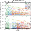 |
Fig. 3. True flux vs redshift for key emission lines in the mock EDS-SFsim (top) and EWS-SFsim (bottom) samples. Contours in dark green, light green, blue, orange, and red correspond to Paβ, Hα, [N II]λ6584, [O III], and Hβ, respectively, selected to span a broad redshift range and wavelength coverage. Each line’s redshift range reflects its detectability within the grism coverage. Contours from lighter to darker shades trace the 99th, 84th, 50th, 16th, and 1st percentiles of the distribution. Grey areas mark fluxes below the survey sensitivity limits. |
4.3. FastSpec spectral by-pass simulations
We converted the incident spectra of MAMBO galaxies into EWS and EDS mock 1D spectra using FastSpec (de la Torre et al., in preparation), a Python-based code that simulates the instrumental and environmental effects on Euclid NISP spectra, bypassing the image-pixel-level approach. Briefly, the FastSpec simulator takes into account effects such as the point-spread function (PSF) model, the spectral extraction window and resulting flux loss, environmental noise from zodiacal background and stray light contribution, as well as instrumental noise factors including readout noise and dark current that have been characterised during NISP ground-based tests (Maciaszek et al. 2022). It also accounts for transmission functions and quantum efficiency, effective collecting surface area, and exposure time of each observation. The strength of a bypass code simulator such as FastSpec lies in its efficiency and short processing times. However, some limitations come into play. We highlight here the most significant ones below:
(1) In slitless spectroscopy, overlapping spectra from nearby objects contribute to noise. Euclid uses a specific observing sequence at four different angles, while FastSpec simplifies this by arranging galaxies on a grid without interference and simulating only first-order spectra. This results in simulated Euclid-like spectra, free from contamination, ensuring fully decontaminated spectral products.
(2) The FastSpec simulator processes a single incident SED per galaxy, limiting its ability to differentiate between bulge and disk components. To accommodate this, we combine bulge and disk MAMBO incident SEDs into a single incident SED. The simulator then convolves this merged SED with the galaxy’s surface brightness profile and instrumental PSF, including background contributions. It models the 2D surface brightness as a composite of two Sérsic profiles, preserving the total luminosity and adjusting contributions based on B/T ratio, inclination, and position angle. Consequently, emission lines are scattered across the galaxy’s 2D spectrum, neglecting spatial variations and spectral contributions from older, centrally-concentrated stellar populations, to disk outskirts where younger stars dominate.
At this stage, we generated red grism 1D spectra for both the EWS and EDS, as well as blue spectra for the DEEP survey, by integrating the individual exposures over the cross-dispersion dimension. We imposed a fixed extraction window of five pixels (equivalent to roughly 1.5 arcseconds), regardless of the galaxy’s size. Consequently, some flux loss is inevitable, that is proportional to the fraction of the galaxy’s light distribution excluded from the extraction aperture. This differs slightly from the Euclid pipeline, which sets the extraction width from the semi-major axis and caps it between 5 and 31 pixels (Euclid Collaboration: Romelli et al. 2026; Euclid Collaboration: Copin et al. 2026), with the lower bound ensuring adequate sampling of the NISP PSF and the upper bound limiting contamination from extended sources.
Figure 4 shows an example spectrum at z ∼ 1.6 from our MAMBO simulation, with both EWS-SFsim and EDS-SFsim realisations. Both EWS-SFsim and EDS-SFsim spectra show a flux loss relative to the incident spectrum, with an average offset of roughly 20% per Å−1, due to the synthetic extraction window we used to derive the 1D spectrum.
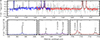 |
Fig. 4. Example of a simulated spectrum from MAMBO of a galaxy at redshift z ∼ 1.6, stellar mass of log10(M*/M⊙) = 10.8, HE ∼ 21.1, SFR of 232.7 M⊙/yr, effective disk radius of |

We note that the continua of the EDS-SFsim and EWS-SFsim realisations in Fig. 4 appear noisy, with the EWS-SFsim spectrum being noisier than the EDS-SFsim one, as expected. Defining the S/N as the flux divided by its associated error, Fig. 5 shows the distribution of the average S/N of the stellar continuum (measured after masking emission lines) for spectra in both samples, including the blue and red grisms for EDS-SFsim. In both cases, the stellar continuum has an average S/N below 1 per Å, emphasising the necessity of stacking Euclid spectra to extract reliable information for non-cosmological studies.
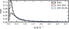 |
Fig. 5. Distribution of the continuum S/N per Å for the sample of simulated MAMBO spectra (see Sect. 4.1), providing a reference for typical input spectra quality. The black line represents the EWS MAMBO sample, selecting galaxies with HE < 24. The red and blue lines correspond to the EDS red and blue MAMBO samples, respectively, selecting galaxies at the survey limit of HE < 26. |
4.4. Redshift and spectral features measurements
Redshifts and emission line properties are measured in simulated spectra with the official Euclid pipeline (Sect. 2).
Figure 6 shows the measured redshift as a function of the true galaxy redshift for both the EWS-SFsim (top panel) and EDS-SFsim (bottom panel) simulations. The distribution of galaxies forms a characteristic spider-web pattern, within which we can qualitatively identify three categories of solutions: (1) accurate redshift measurements, which lie along the bisector of the diagram; (2) misclassified redshift solutions, where the fitting algorithm incorrectly interprets one spectral line as another, producing overdensities along straight lines with slopes distinct from the bisector; and (3) wrong redshift solutions, where noise spikes are mistaken for emission lines, resulting in a scattered distribution with no clear trend all over the parameter space. It is important to note that the EWS results preferentially favour redshift solutions in the range 0.9 ≲ z ≲ 1.8, due to the prior constraints on redshift imposed in the fitting algorithm. We note that, by construction, sources with intrinsically faint or absent emission lines, which are more susceptible to catastrophic redshift failures, are excluded from our mock samples (see Sect. 4.2). As a consequence, the contamination fraction inferred from these simulations, should be interpreted as lower limits, and are further discussed in the following sections.
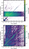 |
Fig. 6. Measured redshift vs true redshift for the mock EWS-SFsim (top panel) and the EDS-SFsim (bottom panel). Bins are colour-coded according to the number counts per deg2. |
5. Redshift contaminants
Stacking is an effective method to create high-S/N spectra for galaxy evolution studies, but its effectiveness heavily relies on the good alignment of the individual spectra, i.e. on the redshift accuracy (|Δz|/(1 + z)). We performed dedicated tests to verify that a redshift accuracy of ≤0.003 represents a suitable compromise for stacking-based galaxy evolution studies. This threshold allows for the inclusion of fainter galaxy populations, despite their lower redshift precision, while still contributing meaningfully to the composite spectra. As a result, we can effectively leverage the capabilities of both the EWS and EDS surveys. A threshold of |Δz|/(1 + z)≤0.003 ensures that, for a galaxy at z ∼ 1.68, the Hα peak is displaced by no more than ±0.53 nm (i.e. about four pixels) from its true centroid. This displacement keeps Hα within the wavelength range of the blended Hα+[N II] lines, minimising the risk of misinterpreting nearby noise spikes as Hα, while also ensuring that we can probe emission line measurements at fainter flux levels using stacking techniques.
All galaxies with |Δz|/(1 + z) > 0.003 are considered redshift contaminants (hereafter simply referred to as contaminants). Before stacking Euclid spectra, we must evaluate the impact of their inclusion on the quality of stacked spectra when Δz/(1 + z) will not be available as in real spectra. In the following, we analyse the two classes of contaminants introduced in Sect. 4.4. These are the spectral line mis-identifications and spurious line detections, where noise spikes are mistaken for emission lines.
5.1. Redshift contaminants from misclassified emission lines
Some contaminant galaxies have incorrect redshift estimates due to the mis-identification of emission lines by the Euclid pipeline. An emission line at rest-frame wavelength  is observed at
  , but if it is mis-identified as another line with rest-frame wavelength
  , the measured redshift becomes
  . The resulting redshift offset is
 (4)
(4)
This implies that misclassified emission lines lead to redshift contaminants with fixed Δz/(1 + z) values, determined solely by the line mis-identification. For example, [S III]λ9531 mis-identified as Hα leads to Δz/(1 + z) = 0.452, and [O III] as Hα gives Δz/(1 + z) = − 0.237.
These contaminants align as straight lines in the zmeas versus ztrue plane (see Fig. 6), with slope  , and intercept
  . To illustrate this, Fig. 7 (left panel) presents an example of such mis-identification in the spectrum of an individual galaxy. Although the spectrum shows multiple (low-S/N) emission lines that could, in principle, be correctly identified, the redshift pipeline incorrectly assigns the redshift likely due to the use of the Hα-based prior (see Sect. 2), which is optimised for the low-SN Hα-dominated sample targeted by the EWS. While such a strategy reflects realistic expectations for automated redshift determination in survey data, it may lead to mis-identifications in cases like these. Improvements could be achieved by retuning the prior for specific samples, but this was not explored in the present study, which relies on the default Euclid pipeline.
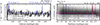 |
Fig. 7. Left panel: Example of redshift contaminants due to [S III]λ9531 at 1752.7 nm mis-identified as Hα, yielding zmeas = 1.67 instead of ztrue = 0.836. Right panel: Median (in blue) and mean (in red) stack of 200 spectra (in grey) of galaxies where the [S III]λ9531 line was misinterpreted as Hα. Vertical dotted lines indicate the ‘true’ lines, while the coloured bands highlight the expected rest-frame positions of key optical emission lines at the wrong redshift of the stacked spectrum (Hβ, [O III], Hα, and [N II]). |
These misclassified sources, if not removed, contaminate the stacked spectra. Since stacking relies on the measured redshift, the spectral features of contaminants are aligned incorrectly, degrading the stacked spectrum by introducing shifted and spurious features. Figure 7 (right panel) shows an example, demonstrating how misclassified [S III]λ9531 lines contaminate the Hα region of a stacked spectrum generated with SpectraPyle by combining 200 individual ‘contaminants’, applying the ‘regular’ normalization with ‘luminosity’ conservation, and omitting sigma clipping (Sect. 3). Additional misplaced spectral features from contaminant spectra can affect regions of the stacked spectrum that are unrelated to key emission lines, thereby degrading the stellar continuum. For instance, features near 450 nm and 625 nm in the stacked spectrum of Fig. 7, originate from interloper galaxy spectra whose emission lines (i.e. Hα+[N II] and [S II] and [S III]λ9069) are redshifted into these observed-frame positions.
5.2. Redshift contaminants from random noise spikes
A significant category of redshift contaminants arises from random noise spikes in the spectra of faint galaxies, which are erroneously interpreted as emission lines. These contaminants result in completely spurious redshift measurements that are unrelated to the true underlying spectra, leading to a broad distribution in Δz/(1 + z) and a random scatter in the zmeas versus ztrue plane.
Figure 8 shows an example of this type of line mis-identification in an individual galaxy (left panel) and in the stacked spectrum of 500 such contaminants (right panel). The purpose of this exercise of stacking only contaminants is to demonstrate the contribution of incorrect redshifts to the overall stacked signal, if they are not properly filtered out. As expected, a spurious Hα emission line emerges in the stacked spectrum. However, a striking feature of the stacked spectrum is the appearance of not only the spurious Hα line but also other emission lines such as Hβ, [O III]λ4959, [O III], and [S II]λλ6716–6731. This is a predictable consequence of the pipeline’s redshift determination method, which fits templates with multiple emission lines. In noisy spectra, random noise spikes can coincidentally align with the expected positions of these lines, leading the algorithm to assign incorrect redshifts. When these mis-identified spectra are stacked, the template features reinforce each other, causing all expected emission lines to appear coherently at the spurious redshift location.
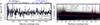 |
Fig. 8. Left panel: Example where a random noise spike is misinterpreted as the Hα emission line, leading to an erroneous redshift measurement. Right panel: Median (in blue) and mean (in red) stacked spectrum of 500 spectra (in grey) of galaxies with misclassified redshift, illustrating the accumulation of these spurious noise spikes at notable lines positions. |
Figure 9 shows the Hα flux distributions (corrected for flux loss, following Cassata et al., in preparation)for the EDS-SFsim (top panel) and the EWS-SFsim (bottom panel). The figure shows the effects of redshift misclassification and noise spikes on Hα measurements, using Hα as a representative example for all spectral lines. Most contaminants exhibit measured fluxes below the flux limits of their respective surveys and could, in principle, be excluded by imposing stricter flux thresholds. However, even when restricting the analysis to galaxies with Hα fluxes above these limits, at the cost of excluding fainter regimes of the scaling relations, a significant fraction of contaminants remains. As shown in Fig. 9, these residual contaminants predominantly contribute low flux values to the stack, thereby their impact on the composite measurements should be limited. This effect will be examined in greater detail in the following sections.
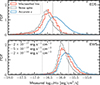 |
Fig. 9. Distribution of measured Hα fluxes (corrected for flux loss following Cassata et al., in prep.) versus true Hα fluxes for the EDS-SFsim (top) and EWS-SFsim (bottom) simulated samples. Blue histograms show galaxies with accurate redshifts with |Δz|/(1 + z)≤0.003, red histograms indicate contaminants from mis-identified emission lines, and grey histograms represent contaminants from noise spikes. |
5.3. Insights on contamination level from high-percentile stacked spectra
To summarise the impact of redshift–contaminant galaxies in the Euclid stacked spectra, Fig. 10 shows a composite constructed from 2642 EWS-SFsim individual spectra. Of these, 51% have reliable redshift measurements, while the remaining 49% are a mixture of various types of redshift contaminants. Misclassified emission lines contribute approximately 8%, consisting of [S III]λ9531 mistaken for Hα, 2% from [O III], and about 1% from [O II], with a further ∼4% arising from less common emission lines. Redshift contaminants caused by noise spikes account for roughly 36%. The mean spectrum demonstrates the resilience of the composite stacking approach, as it is minimally affected by redshift contaminants. However, the percentile composite spectra reveal intriguing features. Notably, above the 90th percentile (and faintly visible also in the 84th percentile composite), spectral features attributed to redshift contaminants emerge. These features include the Hα + [N II] complex and [S II] lines at wavelengths around 452.5 nm and 463.0 nm, respectively, corresponding to contaminants where [S III]λ9531 has been misclassified as Hα. Additionally, the [O II] doublet appears near 490 nm, originating from contaminants where [O III] has been misclassified as Hα.
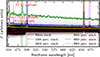 |
Fig. 10. Stacked mean spectrum of simulated MAMBO galaxies from the EWS with stellar masses in the range 1010 M⊙ ≤ M* ≤ 1010.5 M⊙ and redshifts 1.52 ≤ z ≤ 1.86. The stacked is composed of a mixture of 2642 spectra, with contributions from galaxies with accurate redshifts (51%), as well as redshift contaminants arising from noise spikes (36%), [S III]λ9531 misclassified as Hα (8%), and [O III] misclassified as Hα (2%), plus minor contributions from other misclassified emission lines (∼5% in total). The plot includes the mean spectrum (red) and composite spectra at the 16th, 84th, 90th, 98th, and 99th percentiles (brown, orange, yellow, blue, and green, respectively). The contribution of individual galaxy spectra is shown in black. |
This has interesting implications for future studies. The presence of redshift contaminants in the high-percentile composite spectra suggests that stacking analyses may offer a potential diagnostic tool to qualitatively assess sample contamination. While still exploratory, this idea opens the possibility of using statistical or machine learning techniques to analyse flux distributions across percentile composites as a way to characterise contamination. In a future work, we plan to investigate whether specific outlier galaxies contributing to these percentiles can be identified, which may eventually support the development of methods to improve sample selection.
6. Scientific cases
The strength of applying stacking techniques specifically to Euclid is, of course, the enormous total number of spectra that will be available, which will translate into the possibility of creating very high-S/N stacked spectra to explore the physical parameter space of galaxies and AGNs in a very fine grid. To fully exploit this potential, it is essential to first quantify the quality of the input samples in terms of success rate and contamination rate, which determine the balance between completeness and purity. Once these selection metrics are established, we can proceed to analyse the resulting stacked spectra, assessing how the adopted criteria influence the recovery of key spectral features and derived physical quantities.
6.1. Success rate and contamination rate
In this section, we introduce metrics that provide a direct measure of the trade-off between sample completeness and contamination, and are critical for evaluating the reliability of stacked spectra in both the EWS-SFsim and EDS-SFsim configurations. We define the following conditions:
-
z(true): galaxies that actually fall within a certain redshift interval (ztrue ∈ [zmin, zmax]);
-
z(meas): galaxies that are measured to be in the defined redshift interval (zmeas ∈ [zmin, zmax]);
-
z(accur): galaxies satisfying the redshift accuracy requirement (|Δz|/(1 + z)≤0.003);
-
z(prob): galaxies with a zprob (redshift probability) above a certain threshold (between 0 and 1);
-
F(true): galaxies whose line of interest has true flux greater than a given threshold (Ftrue > Fthreshold);
-
F(meas): galaxies whose line of interest has a measured flux greater than the threshold (Fmeas > Fthreshold);
-
S(θ): to take into account additional constraints or conditions. For example, θ could be a condition to select galaxies within a certain stellar mass (as in the following section), or a condition on the minimum S/N of a certain measured spectral feature, etc.
With these definitions, we can express the success rate (𝒮ℛ) as the ratio of galaxies in a certain population that are successfully detected to the total number of such galaxies that exist above the defined thresholds,
![Mathematical equation: $$ \begin{aligned} \mathcal{SR} = \frac{\#\left[ \mathrm{z(meas)} \,{\scriptstyle \& }\, \mathrm{z(accur)} \,{\scriptstyle \& }\, \mathrm{z(prob)} \,{\scriptstyle \& }\, \mathrm{F(true)} \,{\scriptstyle \& }\, \mathrm{F(meas)}\,{\scriptstyle \& }\, \mathrm{S}(\theta )\right]}{\#\left[ \mathrm{z(true)} \,{\scriptstyle \& }\, \mathrm{F(true)} \,{\scriptstyle \& }\, \mathrm{S}(\theta )\right]}\cdot \end{aligned} $$](/articles/aa/full_html/2026/03/aa57329-25/aa57329-25-eq14.gif) (5)
(5)
In particular, we are interested in an EWS sample selected in the redshift interval extended between 0 and 4, including Hα at 0.9 ≲ zmin ≲ 1.8, as well as other emission lines, such as Paβ at lower redshifts or [O II] at higher redshifts. Finally, we aim to reach depth, with thresholds as low as 2 × 10⁻¹⁷ erg s−1 cm−2 in both our surveys.
Similarly, we define the contamination rate (𝒞) as a parameter that quantifies the fraction of misclassified sources relative to the observationally selected sample,
![Mathematical equation: $$ \begin{aligned} \mathcal{C} = \frac{\#\left[\mathrm{z(meas)} \,{\scriptstyle \& }\, \lnot \mathrm{z(accur)} \,{\scriptstyle \& }\, \mathrm{z(prob)} \,{\scriptstyle \& }\, \mathrm{F(meas)}\,{\scriptstyle \& }\, \mathrm{S}(\theta )\right]}{\#\left[ \mathrm{z(meas)}\,{\scriptstyle \& }\, \mathrm{z(prob)} \,{\scriptstyle \& }\, \mathrm{F(meas)} \,{\scriptstyle \& }\, \mathrm{S}(\theta )\right]}\cdot \end{aligned} $$](/articles/aa/full_html/2026/03/aa57329-25/aa57329-25-eq15.gif) (6)
(6)
Here, the symbol ¬ denotes negation, indicating the complement of a condition (e.g. ¬z(accur) represents galaxies that do not satisfy the redshift accuracy requirement).
Finally, we define an optimal observational selection that represents the best selection sample that one can achieve with Euclid for a given redshift range and flux threshold, and with no redshift contaminants. We call this the benchmark sample (ℬℳ), defined as
 (7)
(7)
6.2. Sample selection for stacking
In this section we examine a preliminary finding which will serve as the basis for analysing key scaling relations relevant to galaxy evolution in the following section. Based on the selection criteria detailed in Appendix B, which aim to maximise 𝒮ℛ and minimise 𝒞, the left panels of Fig. 11 show the Hα emission line distribution as a function of stellar mass for the EDS-SFsim selection in the redshift interval 0.9 ≤ zmeas ≤ 1.2. The left panels show the distribution of the ℬℳ sample, galaxies with accurate redshift measurements, and redshift contaminants. For contaminants, the y-axis reflects mis-identified spectral features interpreted as Hα by the pipeline. The top panel shows the relationship at the flux limit of F(Hα)≥2 × 10⁻¹⁷ erg s−1 cm−2 without applying a cut in redshift probability. In contrast, the bottom panel demonstrates the effects introduced by our fiducial selection, which includes a cut at zprob ≥ 0.4. The contours in both panels show the ground-truth distributions for the full EDS-SFsim parent sample (HE ≤ 26) and a subsample with F(Hα) ≥2 × 10⁻¹⁷ erg s−1 cm−2, respectively, along with their median trends. Their comparison highlights a critical limitation: even in the absence of instrumental effects, applying a flux threshold introduces a strong bias towards higher Hα fluxes, particularly at stellar masses below 1010 M⊙. As a result, global scaling relations involving Hα cannot be reliably recovered at low masses using flux-limited samples such as the Euclid spectroscopic selection. This bias is intrinsic to the selection function and not a consequence of the stacking procedure itself. Nevertheless, at stellar masses above 1010 M⊙, the two ground-truth curves agree within 0.05–0.1 dex, suggesting that in this regime it may still be possible, in principle, to recover unbiased global scaling relations involving Hα.
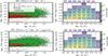 |
Fig. 11. Simulated Hα emission line as a function of stellar mass for the EDS-SFsim selection is shown for the lowest redshift range: 0.9 ≤ zmeas ≤ 1.2. Top panels present the relation at the flux limit of F(Hα)≥2 × 10⁻¹⁷ erg s−1 cm−2 and with no cut in zprob, whilst the bottom panels present the improvement obtained with our fiducial selection that also includes a cut in redshift probability zprob ≥ 0.4. The left panels show the distributions of the different subsamples: the ℬℳ sample (grey points; Eq. (7)), the observationally selected galaxies with accurate redshifts (green points), and the redshift contaminants (red points). Note that the green and red points together constitute the observationally selected sample, as defined by the denominator of Eq. (6). Black and cyan contours and dashed lines show the ground-truth distributions for the full EDS parent sample (HE ≤ 26) and a subsample selected with F(Hα)≥2 × 10⁻¹⁷ erg s−1 cm−2, respectively. These contours serve as a reference to illustrate the intrinsic (ground-truth) distributions, allowing for a qualitative comparison with the observation-like measurements, and to highlight the intrinsic selection bias introduced by the flux limit, which would persist even without redshift measurement errors. The right panels show galaxy number densities per deg2 in bins of stellar mass and Hα flux, with 𝒮ℛ (top number) and 𝒞 (bottom number) indicated. Numbers are colour-coded: black-blue for reliable bins (𝒮ℛ > 45%, 𝒞 < 20%) and red and magenta for others. The numbers reported above each mass bin represent the 𝒮ℛ (top number) and 𝒞 (bottom number) for the entire mass bin. |
Building on this, the bottom panel of Fig. 11 demonstrates that applying a moderate quality cut (zprob > 0.4) reduces the contribution of contaminants while still retaining a high level of completeness. This trade-off is critical to confirm that meaningful statistical trends can be extracted from the flux-limited sample when appropriate quality filters are applied.
To quantitatively assess the effect of this enhancement, we constructed the right panels of Fig. 11, where galaxies are binned in both stellar mass and Hα flux, and colour-coded by surface density. The corresponding 𝒮ℛ and 𝒞 values are reported for each bin, highlighting which regions of parameter space yield reliable measurements: bins with 𝒮ℛ > 45% and 𝒞 < 20% are shown in black and blue, while less reliable bins are shown in red and magenta. This simulation highlights the potential of the full EDS survey to map the Hα–stellar mass relation with high fidelity, with most of the Mass and SFR bin with high completeness and low contamination, in particular if we include a cut on zprob. Covering ∼50 deg2 of sky, the EDS will enable stacking in finer bins than 0.5 dex, thereby boosting the S/N in composite spectra. However, the present mock catalogue, limited to 3.14 deg2, includes fewer galaxies per bin, constraining the achievable S/N. To optimise both the statistical robustness and sample homogeneity, we therefore perform stacking in bins of stellar mass alone, rather than jointly in stellar mass and Hα flux. This choice ensures that each bin retains a representative population while maximising the number of spectra per stack, thus enabling reliable derivation of scaling relations despite the selection effects. Note that 𝒮ℛ and 𝒞 for each stellar mass bin are reported at the top of the figure, being always 𝒮ℛ > 50 − 60% but the most massive bin and 𝒞 < 7% if a zprob cut is used.
Figure 12 shows the Hα emission line as a function of stellar mass for the EWS-SFsim sample. The figure highlights the impact of applying a flux limit of F(Hα) > 2 × 10⁻¹⁶ erg s−1 cm−2, showing a bias between the magnitude-selected sample and the sample with the additional flux limit. This bias is larger than that estimated for the EDS-SFsim sample (Fig. 11), particularly at lower stellar masses. This discrepancy arises due to the brighter flux limit of the EWS-SFsim sample, which inherently excludes a larger fraction of lower-mass, fainter galaxies. The top panels of Fig. 12 show the relationship at the flux limit of F(Hα) > 2 × 10⁻¹⁶ erg s−1 cm−2 without imposing a redshift probability cut. In comparison, the bottom panels highlight the improvements achieved using our fiducial selection (see Appendix B), which applies a cut at zprob ≥ 0.99, demonstrating once more that our refined approach substantially reduces contaminant contributions while preserving an acceptable level of completeness within the regime achievable with the EWS’s sensitivity. Thanks to the vast sky coverage, the EWS will provide large statistical power to investigate scaling relations for galaxies with Hα flux above 2 × 10⁻¹⁶ erg s−1 cm−2. Similarly to the EDS-SFsim, stacking spectra in bins of stellar mass alone, rather than in bins defined by both stellar mass and Hα flux, will optimise the number of galaxies included in each composite spectrum. This approach ensures that, even within the limited volume of our simulation, stacking can yield high-quality composite spectra at the high-flux, high-mass end of Hα scaling relations with high statistical precision. We note that 𝒮ℛ and 𝒞 for each stellar mass bin are reported at the top of the figure, with 𝒮ℛ > 50 − 60% for all but the most massive bin and 𝒞 < 5% if a zprob cut is used.
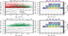 |
Fig. 12. Simulated Hα emission line as a function of stellar mass for the EWS-SFsim selection. Top panels present the relation at the flux limit of F(Hα)≥2 × 10⁻¹⁶ erg s−1 cm−2 and with no cut in zprob, whilst the bottom panels present the improvement obtained with our fiducial selection that also includes also a cut in redshift probability zprob ≥ 0.99. The layout is the same as in Fig. 11, the only difference is that the black and cyan contours and dashed lines show the ground-truth distributions for the full EWS parent sample (HE ≤ 24) and a subsample selected with F(Hα) ≥ 2 × 10⁻¹⁶ erg s−1 cm−2, respectively. Note: in this case, the bias between the cut in magnitude only and the cut in magnitude and flux limit is larger than the EDS-SFsim one. Therefore, even with stacking, we are mapping scaling relations of galaxies with Hα flux above 2 × 10⁻¹⁶ erg s−1 cm−2. |
6.3. Properties of the stacked mock spectra
Building on the selection tests presented in Appendix B and the findings of the previous subsection, we generated stacked spectra using:
-
EWS-SFsim: F > 2 × 10⁻¹⁶ erg s−1 cm−2 and zprob ≥ 0.99;
-
EDS-SFsim: F > 2 × 10⁻¹⁷ erg s−1 cm−2 and zprob ≥ 0.4.
In the case of EDS-SFsim, stacked spectra span three redshift bins ([0.9, 1.2], [1.2, 1.52], and [1.52, 1.86]) and are further divided into stellar mass bins of 0.5 dex, ranging from log10(M*/M⊙)≥8.5 to ≤11.5. For the EWS-SFsim, stacked spectra were created focussing on the redshift bin [1.52, 1.86], where the key emission lines from Hβ to [N II] are present in all spectra. The stacked spectra were produced with SpectraPyle, using the ‘regular’ normalization option with ‘luminosity’ conservation (Sect. 3), applying 4σ sigma clipping to remove outliers, and 350 bootstrap resamplings to estimate uncertainties. All spectra were shifted to the rest frame and resampled at 6 Å per pixel.
Figure 13 shows the rest-frame stacked spectra of galaxies in the redshift bin [1.52, 1.86], for qualitative inspection. The EDS-SFsim stacks have high S/N, whereas the EWS-SFsim stacks, particularly in the lowest mass bins, appear noisier. This difference arises from both the intrinsically higher S/N of individual EDS-SFsim spectra and the limited simulation area of approximately 3 deg2. In the actual EWS survey, the larger sky coverage will yield higher S/N in the stacked spectra. The observationally selected EDS-SFsim spectra closely match their benchmark counterparts, with systematic deviations remaining below 4%, indicating that the adopted selection criteria effectively recover the same underlying galaxy population.
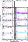 |
Fig. 13. Stacked mean spectra for the mock galaxies used for the scientific predictions in this paper, for the redshift bin [1.52, 1.86]. The panels show stacked spectra divided by sample type and stellar mass bins: left panels show the EDS-SFsim, while right panels show the EWS-SFsim. Rows correspond to stellar mass bins of 0.5 dex, ranging from log10(M*/M⊙)≥8.5 to ≤11.5. Bins with fewer than 50 spectra are not shown or considered in the analysis. In each panel, cyan and magenta spectra represent the stacked spectra for the ℬℳ and observationally selected samples, respectively, with the numbers indicating the spectra counts. Note that the [O III]/[O III]λ4959 ratios of all stacks here are approximately 2.3, lower than the theoretical value of 3, due to an error in the simulated [O III]λ4959 emission line. Since the [O III] values are correct and [O III]λ4959 was not used in the analysis, the results remain unaffected. |
Within each stellar mass bin, the stacked spectra become progressively brighter at lower redshifts, consistent with the reduced distances to these sources from us. Moreover, the continua become redder with increasing stellar mass, which reflects the diminished contribution of blue light from younger stellar populations. The emission line ratios also evolve: the Hα/Hβ ratio increases with stellar mass, suggesting stronger dust attenuation, while the [O III]/Hα ratio decreases, driven by both increased dust extinction and a lower fraction of ionising photons from young stars in more massive galaxies (e.g. Citro et al. 2017). The high S/N of the EDS-SFsim stacks also reveals absorption features such as the NaD doublet around 0.59 μm, which becomes especially prominent at log10(M*/M⊙)≥9.5. Once the full survey area is covered, the enhanced S/N of the stacked spectra will enable the detection of fainter emission and absorption features, expanding the range of scientific analyses that can be pursued with Euclid.
7. Scaling relations with Euclid stacked spectra
In this section, we explore key scaling relations using the most prominent emission lines in the optical domain. The fluxes of these lines were measured in the stacked spectra described in the previous section, using slinefit5 (Schreiber et al. 2018; Talia et al. 2023). This fitting process includes continuum subtraction and deblending of Hα from [N II], ensuring accurate flux measurements. For the EDS-SFsim sample, we focus on the highest redshift bin of the EDS-SFsim selection (1.52 ≤ z ≤ 1.86), which also overlaps with the redshift coverage of the EWS-SFsim sample. Equivalent plots for EDS-SFsim in the lower redshift bins (0.9 ≤ z ≤ 1.2 and 1.2 ≤ z ≤ 1.52) are provided in Appendix C.2.
7.1. Emission lines-to-stellar mass
The fluxes of prominent emission lines measured from stacked mock spectra as a function of stellar mass provide a diagnostic of the performance of the EDS-SFsim selection across redshift and stellar mass bins. Figure 14 presents the fluxes of Hα, Hβ, [O III], and [N II], corrected for flux losses following the methodology outlined in Cassata et al. (in preparation), within the redshift interval 1.52 ≤ z ≤ 1.86. Magenta curves show flux measurements from mean stacks of observationally selected galaxies, while cyan circles represent the mean fluxes from the benchmark (ℬℳ) selection. The difference between these is displayed in the bottom inset of each panel (in purple, in dex), along with the 1σ uncertainties. Across all stellar mass bins, the observational selection reproduces the benchmark fluxes with remarkable fidelity, with typical deviations ranging between 0.001 and 0.06 dex. Notably, the agreement with benchmark values improves at higher stellar masses, particularly above 1010 M⊙, where differences are reduced to between 0.001 and 0.03 dex. The limited impact of residual contaminants on the flux arises because, as shown in Fig. 9, their fluxes generally fall below the surveys’ flux limits, contributing mainly low values to the stack and minimally affecting the composite measurements.
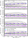 |
Fig. 14. Emission line fluxes (in units of erg s−1 cm−2) measured on stacked spectra as a function of stellar mass for the EDS-SFsim selection corresponding to the redshift interval 1.52 ≤ z ≤ 1.86. From top to bottom, panels show the fluxes of Hα, Hβ, [O III], and [N II] emission lines. Fluxes have been corrected for flux loss using the method by Cassata et al. (in preparation). Magenta curves represent measurements from observationally selected galaxy stacks, whilst cyan circles correspond to benchmark (ℬℳ) stacks. The red dotted horizontal line in each panel indicates the flux limit of 2 × 10⁻¹⁷ erg s−1 cm−2 imposed on the EDS-SFsim. Shaded regions denote the 1σ uncertainty, whilst black contours and the dashed black line in each panel trace the ground-truth distribution and median relation of the parent EDS-SFsim sample (HE ≤ 26), respectively. The bottom insets in each panel show the difference (in dex) between the observational and benchmark flux measurements. |
Black contours and the dashed black line in each panel trace the ground-truth distribution and median relation of the parent EDS-SFsim sample (HE ≤ 26), respectively. The comparison between fluxes measured from the stacked spectra and the photometric ground-truth again highlights the intrinsic bias introduced by the flux-limited selection of EDS-SFsim, which is independent of the stacking process. This bias is especially evident at stellar masses below 1010 M⊙ (see Sect. 6).
For the EWS-SFsim selection, the fluxes of prominent emission lines measured on stacked spectra as a function of the stellar mass are shown in Fig. 15. We find that all lines we analysed, such as Hα, Hβ, [O III], and [N II], show a significant positive bias compared to those of the ground-truth parent sample at HE ≤ 24. These elevated values reflect the more stringent flux limit of 2 × 10⁻¹⁶ erg s−1 cm−2 we imposed on the EWS-SFsim, which preferentially selects galaxies with brighter emission lines (see Sect. 6). The consistently narrow σ uncertainties across all stellar mass bins and emission lines demonstrate the strength of the EWS-SFsim sample in probing bright systems with high statistical precision. This capability is particularly valuable for studying the most active phases of galaxy evolution, such as starbursts, where accurate measurements of emission line properties are essential for constraining physical conditions of the most active star formation phases.
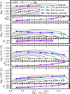 |
Fig. 15. Emission line fluxes measured on stacked mock spectra as a function of stellar mass for the EWS-SFsim selection. From top to bottom, panels display the fluxes of Hα, Hβ, [O III], and [N II] emission lines. The red dotted horizontal line in each panel indicates the flux limit of 2 × 10⁻¹⁶ erg s−1 cm−2 imposed on the Hα line. The layout of the panels is the same as in Fig. 14. |
7.2. The stellar mass attenuation diagram and the Star-formation rate-Stellar mass relation
The main sequence (MS) of SFGs describes a well-established, tight correlation between total stellar mass (M*) of a galaxy and its SFR (e.g. Noeske et al. 2007; Daddi et al. 2007; Wuyts et al. 2011; Rodighiero et al. 2011, 2014; Popesso et al. 2023), showing a clear evolutionary trend across cosmic time.
The Hα emission line, emitted by ionised hydrogen in star-forming regions, is a valuable tracer for measuring the SFR in star-forming galaxies, particularly because it is well-calibrated for use with local galaxies (Kennicutt 1998; Hopkins et al. 2003; Kennicutt & Evans 2012), and can be observed in surveys like the EWS at redshifts 0.9 < z < 1.8 and the EDS at redshifts 0.4 < z < 1.8. By leveraging these observations, we can potentially extend the main sequence characterization to earlier epochs, providing insights into the star-formation history and the evolving galaxy population over time and extending it to the most massive galaxies.
Figure 16 shows the attenuation–M* relation (top panels) and the SFR–M* relation (bottom panels) derived from the EDS-SFsim stacked mock spectra. The attenuation, represented by the Balmer decrement (Hα/Hβ ratio not corrected for underlying Balmer absorption), shows a dependence on stellar mass, with higher attenuation observed at higher masses. In parallel, the SFR–stellar mass relation highlights the ability of the EDS to probe star-forming galaxies at stellar masses above ∼1010 M⊙, where the measured SFR closely aligns with the expected relation for all galaxies with HE < 26. However, for galaxies in the lower-mass regime (< 1010 M⊙), deviations of up to 1 dex below the expected SFR–M* relation are evident. This discrepancy suggests that while the deeper flux limits of the EDS improve the sensitivity to lower-mass systems compared to the EWS, systematic offsets remain, due to the flux limit of the survey as evident from Fig. 14.
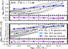 |
Fig. 16. Attenuation–M* relation (top panels) and the SFR–M* relation (bottom panels) derived from the EDS-SFsim stacked spectra. The attenuation is measured using the Balmer decrement (Hα/Hβ ratio), while the SFR is calculated from the dust-corrected Hα luminosity, applying the Calzetti et al. (2000) extinction law and assuming case B recombination conditions (electron density of 100 cm−2 and 10 000 K. The panel layout follows the structure of Fig. 14. Shaded regions represent the 1σ uncertainties in the measured quantities. |
Figure 17 shows the attenuation–stellar mass relation (top panels) and the SFR–M* relation (bottom panels) derived from the EWS-SFsim stacked spectra. For the EWS-SFsim sample, the attenuation–stellar mass relation derived from the Balmer decrement (Hα/Hβ ratio) overlaps with the reference relation of the HE ≤ 24 sample. This agreement indicates that the corrections for dust extinction applied to Hα fluxes from the stacked spectra align closely with those of the reference sample, ensuring comparable dust attenuation estimates. Consequently, the SFRs derived for the EWS-SFsim reflect similar biases to those observed in the Hα flux versus stellar mass relation, as presented in the top panel of Fig. 15. This reinforces that while the EWS-SFsim expands the reach of the survey to larger sky areas, the derived SFR scaling relations remain systematically affected by the high Hα flux limit relative to the benchmark magnitude-limited sample at all stellar masses, and especially at the low-mass end.
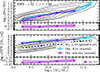 |
Fig. 17. Attenuation–M* relation (top panel) and the SFR–M* relation (bottom panel) derived from the EWS-SFsim stacked mock spectra. The attenuation is measured using the Balmer decrement (Hα/Hβ ratio), whilst the SFR is calculated from the dust-corrected Hα luminosity, applying the Calzetti et al. (2000) extinction law and assuming case B recombination conditions (electron density of 100 cm−2 and temperature of 10 000 K. The panel layout follows the structure of Fig. 14. Shaded regions represent the 1σ uncertainties in the measured quantities. |
7.3. The BPT diagram
Diagnostic diagrams that combine two emission-line ratios are capable of distinguishing the dominant ionising sources in galaxies, whether from young, massive stars formed in recent star formation (SF) or from an AGN. The well-known Baldwin–Phillips–Terlevich (BPT) diagrams (Baldwin et al. 1981; Veilleux & Osterbrock 1987), which compare the ratios [O III]λ5007/Hβ with [N II]λ6584/Hα, [S II]λ6724/Hα, and [O I]λ6300/Hα, have proven effective for differentiating ionising sources in nearby galaxies (Kewley et al. 2001; Kauffmann et al. 2003), while it remains uncertain whether the BPT diagrams will maintain their effectiveness at higher redshifts. As galaxies evolve, their physical conditions and chemical compositions change, potentially complicating the interpretation of these traditional diagnostic diagrams in the distant Universe. Euclid will allow us to extend with unprecedented statistics previous studies using only a small sample observed within the Fiber Multi-Object Spectrograph (FMOS)-COSMOS survey (Kashino et al. 2019) and the MOSFIRE Deep Evolution Field (MOSDEF) survey with Keck by Kriek et al. (2015) and Reddy et al. (2015) in the redshift range 1.4 < z < 1.7. Further studies are indeed required to assess whether these diagnostic tools can reliably classify ionising sources in high-redshift galaxies.
In Fig. 18, we analyse the EDS-SFsim BPT-[N II]λ6584, which relates the [O III]/Hβ and [N II]λ6584/Hα ratios to the ionization mechanisms galaxies. In this analysis, the top and middle panels show the relations between these emission line ratios and stellar mass, based on stacked spectra from the EDS-SFsim sample, in the redshift bin 1.52 ≤ z ≤ 1.86.
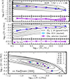 |
Fig. 18. BPT diagram and corresponding stellar mass relations for the [O III]/Hβ and [N II]λ6584/Hα ratios based on the EDS-SFsim stacked mock spectra. Top and middle panels show the [O III]/Hβ–stellar mass (i.e. the MEx diagnostic diagram, Juneau et al. 2011), and [N II]λ6584/Hα–stellar mass relations, respectively, with measurements from the stacked spectra in different stellar mass bins. The bottom panel displays the BPT diagram with symbols representing the positions of the stacked spectra for various mass bins. The black contours in all panels represent the EDS-SFsim parent sample cut at HE ≤ 26, and the black dashed curves in the top and middle panels represent its median relations. |
The [O III]/Hβ ratio has been shown to be a reliable proxy for the ionization parameter U, which traces the current ionization state in star-forming regions (e.g. Citro et al. 2017; Quai et al. 2018, 2019). It is also useful for distinguishing between ionization driven by recent star formation and that dominated by AGN activity, especially when contrasted against stellar mass, as demonstrated by the stellar mass-excitation (MEx) diagnostic (e.g. Juneau et al. 2011), which we employ in this paper. We observe that the [O III]/Hβ ratio in the stacked spectra aligns closely with the median values from the EDS parent sample cut at HE ≤ 26, as indicated by the black dashed curve, across nearly all mass bins. In contrast, the [N II]λ6584/Hα ratio shows a small systematic positive offset from the relation for galaxies with HE < 26. This offset might be either a genuine difference between the [N II]λ6584/Hα in the selected and reference populations, or due to an imperfect deblending of the Hα and the [N II] lines, which may still be affecting the measurement of the [N II] flux.
Now examining the [O III]/Hβ and [N II]λ6584/Hα ratios together in the bottom panel of Fig. 18, the data points in the BPT diagram remain below the Kauffmann et al. (2003) curve, placing them in the region associated with star formation. This indicates that the dominant ionization source in the stacked spectra is star formation, as expected because our MAMBO selection does not include AGN contribution. While there may be biases in individual measurements, particularly in the [N II]λ6584/Hα ratio as discussed above, this does not compromise the overall conclusion. The data consistently support that stacking is robust enough to preserve the position of galaxies even in BPT-[N II] diagram potentially affected by deblending issues.
The stacked EWS-SFsim points in the BPT diagram (Fig. 19) appear slightly closer to the Kauffmann et al. (2003) demarcation line than the EDS-SFsim and the parent population. This offset is mainly due to an overestimation of the [O III]/Hβ ratio in the EWS-SFsim stacks. The effect likely reflects (i) the smaller number of EWS spectra in our simulated 3 deg2 field, which limits the continuum S/N and affects the stellar-continuum subtraction beneath Hβ, and (ii) the statistical nature of the flux-loss correction applied to Hβ, which is derived from a relatively small number of high-S/N spectra. In real Euclid data, the much larger survey area and the availability of reliable reference samples will allow these effects to be better constrained, leading to a more accurate characterisation of the BPT diagram for EWS galaxies.
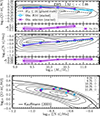 |
Fig. 19. BPT diagram and corresponding stellar mass relations for the [O III]/Hβ and [N II]λ6584/Hα ratios based on the EWS-SFsim stacked mock spectra. Top and middle panels show the [O III]/Hβ-M* (i.e. the MEx diagnostic diagram, Juneau et al. 2011), and [N II]λ6584/Hα-M* relations, respectively, with measurements from the stacked spectra in different stellar mass bins. The bottom panel shows the BPT diagram with symbols representing the positions of the stacked spectra for various mass bins. The black contours in all panels represent the EWS-SFsim parent sample cut at HE ≤ 24, and the black dashed curves in the top and middle panels represent its median relations. |
7.4. The gas-phase metallicity
Gas-phase metallicity, often expressed as the oxygen-to-hydrogen ratio (O/H), is a tracer of galaxy evolution, reflecting the integrated effects of star formation, gas inflows, and outflows over cosmic time. It plays a role in shaping the emission spectrum of ionised gas in galaxies, influencing the strength and ratios of nebular emission lines. Understanding gas-phase metallicity provides insights into chemical enrichment processes and the baryon cycle within galaxies (e.g. Kewley et al. 2019; Maiolino & Mannucci 2019).
Oxygen abundance is commonly estimated using strong line diagnostics calibrated against either direct temperature (Te) measurements or photoionization models. One widely used diagnostic is the O3N2 parameter, defined as ([O III]/Hβ)/([N II]λ6584/Hα), which serves as an effective method for estimating metallicity, especially in galaxies where direct methods are impractical due to the faintness of the auroral lines required to determine Te. These calibrations, based on observations of local galaxies (e.g. Curti et al. 2017), should not be blindly applied to higher redshift, as several studies suggest that O/H evolves with redshift (e.g. Curti et al. 2024; Sanders et al. 2024). To address this, Euclid Collaboration: Scharré et al. (2024) provided guidelines from semi-empirical methods for adjusting metallicity calibrations for high-redshift galaxies. However, the MAMBO simulation adopts the metallicity calibration from Curti et al. (2017) for its modelled galaxies. Consequently, we derive 12+log10(O/H) values for our stacked spectra and analyse how they vary with stellar mass (for both EDS-SFsim and EWS-SFsim) and redshift (for EDS-SFsim).
The results regarding the EDS-SFsim are shown in Fig. 20. First, we observe an almost perfect agreement between the observationally selected samples (purple) and the corresponding benchmark samples (cyan), indicating that we can fully recover the information up to the instrument’s limits. Compared to the HE < 26, our analysis reveals systematic trends in gas-phase metallicity with M*, consistent with the mass-metallicity relation (MZR). At lower stellar masses, metallicities derived from O3N2 tend to be overestimated in all the three redshift bins analysed, potentially due to biases in the calibration or contamination from emission-line ratios influenced by different ionization conditions. Conversely, at higher stellar masses (M★ > 1010 M⊙), metallicities are either consistent with expectations or slightly underestimated.
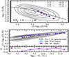 |
Fig. 20. Top panels: O3N2 as a tracer of the gas-phase metallicity 12+log10(O/H) parameter for the EDS-SFsim, in the redshift bin [1.52, 1.86]. The O3N2 values for stacked mock spectra in this study are calibrated using the Curti et al. (2017) relation. The layout of the panels is consistent with the bottom panel of Fig. 18. Bottom panels: Mass-metallicity relation (MZR), showing the dependence of gas-phase metallicity (inferred from O3N2) on stellar mass. The layout matches Fig. 14. |
The corresponding results for the EWS-SFsim are shown in Fig. 21. Here, the difference between the observationally selected and benchmark samples is of the order of 0.01 dex, comparable to what is observed for the EDS-SFsim. However, a systematic bias emerges at higher stellar masses with respect to the parent population (HE < 24), with the stacked values of 12+log10(O/H) systematically lower than those of the parent relation. Given the limitations discussed above, particularly the difficulty of reliably fitting the stellar continuum in the EWS-SFsim spectra due to the limited S/N, this bias remains difficult to interpret. This limitation hampers our ability to determine whether the observed offset arises from the imposed flux-limit and redshift-probability cuts or from measurement uncertainties. A larger dataset, allowing for higher S/N stacks and more accurate continuum subtraction, will be necessary to properly quantify these effects. Such improvements are expected with the availability of a robust reference sample in the real Euclid data and in future data releases.
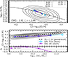 |
Fig. 21. Top panel: O3N2 as a tracer of the gas-phase metallicity 12+log10(O/H) parameter for the EWS-SFsim. The O3N2 values for stacked mock spectra in this study are calibrated using the Curti et al. (2017) relation. The layout of the panels is consistent with the bottom panel of Fig. 18. Bottom panel: Mass-metallicity relation (MZR), representing the dependence of gas-phase metallicity (inferred from O3N2) on stellar mass. The layout matches Fig. 14. |
8. Summary and conclusions
In this preparatory paper for Euclid’s non-cosmological science, we have developed and tested a dedicated stacking pipeline tailored for the Euclid mission’s NISP spectroscopic surveys. Our goal is to recover faint spectral features from large galaxy samples in the Euclid Wide and Deep Surveys (EWS, and EDS, respectively).
To perform the stacking, we released the dedicated code SpectraPyle (see Sect. 3) on the ESA Datalabs platform, accessible to the Euclid Consortium. SpectraPyle’s modular design allows for flexible configurations tailored to diverse scientific objectives, while its computational efficiency supports large dataset processing, essential for Euclid’s extensive sky coverage (see Sect. 3). The method involves selecting suitable input spectra, aligning them to a common reference frame, applying normalization procedures chosen by the users among several possibilities. Then, it combines the data statistically to produce high-quality composite spectra.
Our workflow was applied to two sets of simulated spectra generated with the MAMBO simulation and processed to match Euclid specifications using the FastSpec code. The resulting datasets, EWS-SFsim and EDS-SFsim, correspond to the EWS and EDS, respectively, and are designed to represent the final surveys quality, assuming that known systematics, such as zeroth-order residuals, persistence, and contamination from neighbours, are fully masked and corrected in future pipeline releases, and that flux losses are accounted for, achieving the fidelity expected from an optimal extraction of Euclid spectra.
The analysis began with redshift and flux measurements for each simulated spectrum using the automated fitting procedure of Euclid pipeline, described in Sect. 4.4. We then performed tests aimed at characterising the best selection, to maximise performances in terms of retaining high success rate (𝒮ℛ), whilst limiting the contamination rate (𝒞) for both samples. Our results indicate that a residual percentage of redshift contaminants survive even after rigorous quality cuts (see Appendix B). This underscores the need for careful interpretation and additional refinement of selection methods when analysing stacked Euclid spectra. For the EDS-SFsim, we obtain a fiducial selection with 𝒮ℛ between ∼% and ∼70% and 𝒞 < 6%, while for the fiducial EWS-SFsim sample we find 𝒮ℛ between ∼50% and ∼80% and 𝒞 < 4.5%. At these levels, stacking delivers high-quality spectra of the benchmark (ℬℳ) sample down to log10(M*/M⊙)≃8.5 in the EDS-SFsim and log10(M*/M⊙)≃9.0 in the EWS-SFsim, allowing for a robust reconstruction of galaxy spectra and emission line fluxes and therefore the derivation of physical parameters such as star formation rate (SFR), dust attenuation, and gas-phase metallicity. The key to this performance is that noise contaminants have significantly lower measured Hα fluxes than galaxies with accurate redshifts (Fig. 9), so their impact on the stacks is minimal.
We investigated the nature of stacked spectra for different categories of redshift contaminants. Redshift contaminants arise from various sources, including spikes of noise misinterpreted as Hα, as well as mis-identifications of spectral lines (e.g. [S III]λ9531 and [O III]) being erroneously attributed to Hα. Stacking spectra that consist purely of noise spikes naturally reproduce the features of the template used for galaxy redshift measurements (Sect. 5.2), confirming that such contaminants do contribute to the recovered line fluxes. However, their impact is not catastrophic, as they exhibit significantly lower measured Hα fluxes than galaxies with accurate redshifts, as noted above. Contaminants produced by misclassified emission lines introduce spurious flux at the wavelengths of the line they were mistaken for, with the contamination amplitude scaling with the intrinsic strength of the mis-identified line (a dependence that may differ between our simulations and real data). Also, since the whole spectrum is shifted to the wrong redshift, additional emission features from those interloper spectra can produce further spurious signals in the stacked continuum and at other line wavelengths (see Sect. 5.1). Mis-identified redshift contaminants, however, can be recognised in higher-order percentiles of the stack, where faint but coherent features appear at wavelengths corresponding to the misinterpreted lines (Sect. 5.3). This could provide a useful diagnostic for their identification in real data.
By exploiting the clean benchmark stacks, we show that it is possible to recover fluxes for secondary lines such as Hβ, [O III], and [N II] at levels well below the individual detection limit (Figs. 14–15). This capability can, in principle, be extended to even fainter lines, significantly expanding the range of physical diagnostics accessible through stacking.
We also quantified the important limitations due to selection effects. In particular, the flux-limited nature of the spectroscopic samples that prevents the measurement of the redshift at fainter fluxes, introduces biases that affect the recovery of global scaling relations, such as SFR–M* and attenuation–M*. As demonstrated in Sect. 6, these biases are not caused by the stacking technique itself, but are inherent to the input spectroscopic sample. For the EDS-SFsim, the deeper flux limit enables a recovery of scaling relations that more closely match those of the parent sample, thanks to the higher completeness in redshift measurements, particularly at the high-mass end (M* ≳ 1010 M⊙), where the effects of incompleteness are minimised. In contrast, for the EWS-SFsim, the selection restricts analysis to the bright upper envelope of such relations at all masses, preventing a full characterization of the underlying population. These findings underscore the need for caution when interpreting trends from flux-limited samples and emphasise the critical role of careful quality cuts and completeness assessments in deriving reliable conclusions from stacked spectra.
It is important to emphasise that these results are derived from controlled simulations designed to emulate the final Euclid survey data, after a full pipeline optimisation and removal of known artefacts. The mocks do not include truly passive galaxies or other line-poor systems, whose presence in real observations would likely increase contamination rates and amplify certain biases. Current Q1 Euclid spectra still contain residual systematics from zeroth order, persistence, and contamination; however, these are expected to be substantially mitigated in forthcoming pipeline releases through improved extraction algorithms and more aggressive masking. Our conclusions should therefore be viewed as representative of the survey’s ultimate performance, rather than of current early data products.
Acknowledgments
The Euclid Consortium acknowledges the European Space Agency and a number of agencies and institutes that have supported the development of Euclid, in particular the Agenzia Spaziale Italiana, the Austrian Forschungsförderungsgesellschaft funded through BMIMI, the Belgian Science Policy, the Canadian Euclid Consortium, the Deutsches Zentrum für Luft- und Raumfahrt, the DTU Space and the Niels Bohr Institute in Denmark, the French Centre National d’Etudes Spatiales, the Fundação para a Ciência e a Tecnologia, the Hungarian Academy of Sciences, the Ministerio de Ciencia, Innovación y Universidades, the National Aeronautics and Space Administration, the National Astronomical Observatory of Japan, the Netherlandse Onderzoekschool Voor Astronomie, the Norwegian Space Agency, the Research Council of Finland, the Romanian Space Agency, the State Secretariat for Education, Research, and Innovation (SERI) at the Swiss Space Office (SSO), and the United Kingdom Space Agency. A complete and detailed list is available on the Euclid web site (www.euclid-ec.org). S.Q., L.P., M.T., B.G., A.E., E.D., V.A., G.D.L., H.D. acknowledge support from the ELSA project. ‘ELSA: Euclid Legacy Science Advanced analysis tools’ (Grant Agreement no. 101135203) is funded by the European Union. Views and opinions expressed are however those of the author(s) only and do not necessarily reflect those of the European Union or Innovate UK. Neither the European Union nor the granting authority can be held responsible for them. UK participation is funded through the UK HORIZON guarantee scheme under Innovate UK grant 10093177. V.A. and E.L. acknowledge the support from the INAF Large Grant ‘AGN & Euclid: a close entanglement’ Ob. Fu. 01.05.23.01.14. C.S. acknowledges the support of NASA ROSES Grant 12-EUCLID11-0004 M.S. acknowledges support by the State Research Agency of the Spanish Ministry of Science and Innovation under the grants ‘Galaxy Evolution with Artificial Intelligence’ (PGC2018-100852-A-I00) and ‘BASALT’ (PID2021-126838NB-I00) and the Polish National Agency for Academic Exchange (Bekker grant BPN/BEK/2021/1/00298/DEC/1). This work was partially supported by the European Union’s Horizon 2020 Research and Innovation program under the Maria Sklodowska-Curie grant agreement (No. 754510). L.R. acknowledges support from the Next Generation EU funds within the National Recovery and Resilience Plan (PNRR), Mission 4 – Education and Research, Component 2 – From Research to Business (M4C2), Investment Line 3.1 – Strengthening and creation of Research Infrastructures, Project IR0000034 – “STILES - Strengthening the Italian Leadership in ELT and SKA”.
References
- Angulo, R. E., & White, S. D. M. 2010, MNRAS, 405, 143 [NASA ADS] [Google Scholar]
- Baldwin, J. A., Phillips, M. M., & Terlevich, R. 1981, PASP, 93, 5 [Google Scholar]
- Bezanson, R., van der Wel, A., Straatman, C., et al. 2018, ApJ, 868, L36 [NASA ADS] [CrossRef] [Google Scholar]
- Bruzual, G., & Charlot, S. 2003, MNRAS, 344, 1000 [NASA ADS] [CrossRef] [Google Scholar]
- Calzetti, D., Armus, L., Bohlin, R. C., et al. 2000, ApJ, 533, 682 [NASA ADS] [CrossRef] [Google Scholar]
- Chabrier, G. 2003, PASP, 115, 763 [Google Scholar]
- Choi, J., Conroy, C., Moustakas, J., et al. 2014, ApJ, 792, 95 [Google Scholar]
- Citro, A., Pozzetti, L., Moresco, M., & Cimatti, A. 2016, A&A, 592, A19 [NASA ADS] [CrossRef] [EDP Sciences] [Google Scholar]
- Citro, A., Pozzetti, L., Quai, S., et al. 2017, MNRAS, 469, 3108 [Google Scholar]
- Curti, M., Cresci, G., Mannucci, F., et al. 2017, MNRAS, 465, 1384 [Google Scholar]
- Curti, M., Maiolino, R., Curtis-Lake, E., et al. 2024, A&A, 684, A75 [NASA ADS] [CrossRef] [EDP Sciences] [Google Scholar]
- Daddi, E., Dickinson, M., Morrison, G., et al. 2007, ApJ, 670, 156 [NASA ADS] [CrossRef] [Google Scholar]
- De Lucia, G., Tornatore, L., Frenk, C. S., et al. 2014, MNRAS, 445, 970 [Google Scholar]
- Euclid Collaboration (Scaramella, R., et al.) 2022, A&A, 662, A112 [NASA ADS] [CrossRef] [EDP Sciences] [Google Scholar]
- Euclid Collaboration (Gabarra, L., et al.) 2023, A&A, 676, A34 [NASA ADS] [CrossRef] [EDP Sciences] [Google Scholar]
- Euclid Collaboration (Scharré, L., et al.) 2024, A&A, 689, A276 [CrossRef] [EDP Sciences] [Google Scholar]
- Euclid Collaboration (Cropper, M., et al.) 2025, A&A, 697, A2 [Google Scholar]
- Euclid Collaboration (Jahnke, K., et al.) 2025, A&A, 697, A3 [Google Scholar]
- Euclid Collaboration (Mellier, Y., et al.) 2025, A&A, 697, A1 [Google Scholar]
- Euclid Collaboration (Selwood, M., et al.) 2025, A&A, 693, A250 [Google Scholar]
- Euclid Collaboration (Copin, Y., et al.) 2026, A&A, in press, https://doi.org/10.1051/0004-6361/202554627 [Google Scholar]
- Euclid Collaboration (Le Brun, V., et al.) 2026, A&A, in press, https://doi.org/10.1051/0004-6361/202554607 [Google Scholar]
- Euclid Collaboration (Matamoro Zatarain, T., et al.) 2026, A&A, in press, https://doi.org/10.1051/0004-6361/202554619 [Google Scholar]
- Euclid Collaboration (Romelli, E., et al.) 2026, A&A, in press, https://doi.org/10.1051/0004-6361/202554586 [Google Scholar]
- Francis, P. J., Hewett, P. C., Foltz, C. B., et al. 1991, ApJ, 373, 465 [NASA ADS] [CrossRef] [Google Scholar]
- Girelli, G. 2021, Ph.D. Thesis, Alma Mater Studiorum– University of Bologna [Google Scholar]
- Girelli, G., Bolzonella, M., & Cimatti, A. 2019, A&A, 632, A80 [NASA ADS] [CrossRef] [EDP Sciences] [Google Scholar]
- Gordon, K. D. 2024, J. Open Source Softw., 9, 7023 [NASA ADS] [CrossRef] [Google Scholar]
- Henriques, B. M. B., White, S. D. M., Thomas, P. A., et al. 2015, MNRAS, 451, 2663 [Google Scholar]
- Hirschmann, M., De Lucia, G., & Fontanot, F. 2016, MNRAS, 461, 1760 [Google Scholar]
- Hopkins, A. M., Miller, C. J., Nichol, R. C., et al. 2003, ApJ, 599, 971 [Google Scholar]
- Ilbert, O., McCracken, H. J., Le Fèvre, O., et al. 2013, A&A, 556, A55 [NASA ADS] [CrossRef] [EDP Sciences] [Google Scholar]
- Juneau, S., Dickinson, M., Alexander, D. M., & Salim, S. 2011, ApJ, 736, 104 [Google Scholar]
- Kashino, D., Silverman, J. D., Sanders, D., et al. 2019, ApJS, 241, 10 [Google Scholar]
- Kauffmann, G., Heckman, T. M., Tremonti, C., et al. 2003, MNRAS, 346, 1055 [Google Scholar]
- Kennicutt, R. C., Jr. 1998, ARA&A, 36, 189 [Google Scholar]
- Kennicutt, R. C., & Evans, N. J. 2012, ARA&A, 50, 531 [NASA ADS] [CrossRef] [Google Scholar]
- Kewley, L. J., Dopita, M. A., Sutherland, R. S., Heisler, C. A., & Trevena, J. 2001, ApJ, 556, 121 [Google Scholar]
- Kewley, L. J., Nicholls, D. C., & Sutherland, R. S. 2019, ARA&A, 57, 511 [Google Scholar]
- Kriek, M., Shapley, A. E., Reddy, N. A., et al. 2015, ApJS, 218, 15 [NASA ADS] [CrossRef] [Google Scholar]
- Lang, P., Wuyts, S., Somerville, R. S., et al. 2014, ApJ, 788, 11 [NASA ADS] [CrossRef] [Google Scholar]
- Laureijs, R., Amiaux, J., Arduini, S., et al. 2011, ESA/SRE(2011) 12 [arXiv:1110.3193] [Google Scholar]
- López-López, X., Bolzonella, M., Pozzetti, L., et al. 2024, A&A, 691, A136 [NASA ADS] [CrossRef] [EDP Sciences] [Google Scholar]
- Maciaszek, T., ealet, A., Gillard, W., et al. 2022, in Space Telescopes and Instrumentation 2022: Optical, Infrared, and Millimeter Wave, eds. L. E. Coyle, M. D. Perrin, S. Matsuura, et al. (International Society for Optics and Photonics (SPIE)), 12180, 1K [Google Scholar]
- Maiolino, R., & Mannucci, F. 2019, A&ARv, 27, 3 [Google Scholar]
- Navarro, V., del Rio, S., Angel Diego, M., et al. 2024, in Space Data Management. Studies in Big Data, 141, 1 [Google Scholar]
- Noeske, K. G., Weiner, B. J., Faber, S. M., et al. 2007, ApJ, 660, L43 [CrossRef] [Google Scholar]
- Osterbrock, D. E. 1989, Astrophysics of Gaseous Nebulae and Active Galactic Nuclei (Sausalito, CA: University Science Books) [Google Scholar]
- Peng, Y.-J., Lilly, S. J., Kovač, K., et al. 2010, ApJ, 721, 193 [Google Scholar]
- Popesso, P., Concas, A., Cresci, G., et al. 2023, MNRAS, 519, 1526 [Google Scholar]
- Pozzetti, L., Hirata, C. M., Geach, J. E., et al. 2016, A&A, 590, A3 [NASA ADS] [CrossRef] [EDP Sciences] [Google Scholar]
- Quai, S., Pozzetti, L., Citro, A., Moresco, M., & Cimatti, A. 2018, MNRAS, 478, 3335 [Google Scholar]
- Quai, S., Pozzetti, L., Moresco, M., et al. 2019, MNRAS, 490, 2347 [CrossRef] [Google Scholar]
- Racca, G. D., Laureijs, R., Stagnaro, L., et al. 2016, Space Telescopes and Instrumentation 2016: Optical, Infrared, and Millimeter Wave, 9904, 99040O [Google Scholar]
- Reddy, N. A., Kriek, M., Shapley, A. E., et al. 2015, ApJ, 806, 259 [NASA ADS] [CrossRef] [Google Scholar]
- Rodighiero, G., Daddi, E., Baronchelli, I., et al. 2011, ApJ, 739, L40 [Google Scholar]
- Rodighiero, G., Renzini, A., Daddi, E., et al. 2014, MNRAS, 443, 19 [Google Scholar]
- Sanders, R. L., Shapley, A. E., Topping, M. W., Reddy, N. A., & Brammer, G. B. 2024, ApJ, 962, 24 [NASA ADS] [CrossRef] [Google Scholar]
- Schmitt, A., Arnouts, S., Borges, R., et al. 2019, PASP, 521, 398 [Google Scholar]
- Schreiber, C., Pannella, M., Elbaz, D., et al. 2015, A&A, 575, A74 [NASA ADS] [CrossRef] [EDP Sciences] [Google Scholar]
- Schreiber, C., Elbaz, D., Pannella, M., et al. 2017, A&A, 602, A96 [NASA ADS] [CrossRef] [EDP Sciences] [Google Scholar]
- Schreiber, C., Glazebrook, K., Nanayakkara, T., et al. 2018, A&A, 618, A85 [NASA ADS] [CrossRef] [EDP Sciences] [Google Scholar]
- Scoville, N., Abraham, R. G., Aussel, H., et al. 2007, ApJS, 172, 38 [NASA ADS] [CrossRef] [Google Scholar]
- Springel, V., White, S. D. M., Jenkins, A., et al. 2005, Nature, 435, 629 [Google Scholar]
- Talia, M., Schreiber, C., Garilli, B., et al. 2023, A&A, 678, A25 [NASA ADS] [CrossRef] [EDP Sciences] [Google Scholar]
- Vanden Berk, D. E., Richards, G. T., Bauer, A., et al. 2001, AJ, 122, 549 [Google Scholar]
- Veilleux, S., & Osterbrock, D. E. 1987, ApJS, 63, 295 [Google Scholar]
- Wuyts, S., Förster Schreiber, N. M., van der Wel, A., et al. 2011, ApJ, 742, 96 [NASA ADS] [CrossRef] [Google Scholar]
- York, D. G., Adelman, J., John, E., Anderson, J., et al. 2000, AJ, 120, 1579 [NASA ADS] [CrossRef] [Google Scholar]
The ESA Datalabs are available at https://datalabs.esa.int/.
The code is currently accessible to a limited number of users and will be released to the entire Euclid Consortium prior to publication. Interested researchers in the consortium may contact the authors by email to request early access.
A MAMBO catalogue including AGNs is presented in López-López et al. (2024).
The MAMBO procedure and recipes used to assign fluxes for different emission lines are described here: https://github.com/xalolo/MAMBO.
The slinefit code is publicly available at https://github.com/cschreib/slinefit
The SAS is available at https://eas.esac.esa.int/.
Appendix A: Additional notes on the stacking procedure
A.1. Test on the ‘flux conservation’ method
In Sect. 3.1 we mentioned the limitations of the ‘flux conservation’ method. For a more quantitative assessment, we conducted tests using toy RGS spectra consisting of a flat, noiseless continuum at 2 × 10⁻¹⁸ erg s−1 cm−2 Å−1 (comparable to the average continuum in Fig. 4) and a noiseless Hα Gaussian line with a flux of 2 × 10⁻¹⁶ erg s−1 cm−2. Redshifts were randomly drawn from uniform distributions within various intervals in the range 0.9 ≤ z ≤ 1.8, where Hα falls in the Euclid RGS. We then stacked these spectra at the sample average redshift and analysed the resulting composite spectra. We found that the Hα luminosities in the stacked spectra deviated from the expected average by up to 10%, demonstrating the limitations of this approach for luminosity-sensitive analyses.
A.2. Caveats on the geometric mean
One of the spectral combination options offered by SpectraPyle is the geometric mean, defined by
 (A.1)
(A.1)
where Fλ, i is the flux density of the i-th spectrum in the bin centred on wavelength λ, and n is the number of spectra contributing to the bin. Vanden Berk et al. (2001) has shown that the geometric mean preserves the global continuum shape, which is useful, for example, when analysing spectra with power laws (often used to approximate quasar continua), whereas neither the median nor the mean typically yields a power law with the mean index. Instead, the geometric mean correctly yields a composite power law whose spectral index is equal to the arithmetic mean of the frequency power-law indices. Furthermore, according to the definition in Eq. (A.1), the geometric mean is less likely to be dominated by the brightest spectra than the arithmetic mean. Therefore, in many astrophysical applications involving samples of galaxies with fluxes covering a large dynamical range, the geometric mean should be favoured. However, Euclid spectra, especially the EWS spectra, have a low S/N, and sometimes their flux values subtracted from the background are less than zero. Therefore, the geometric mean cannot be used in these cases as it is only defined for positive values.
A.3. SpectraPyle performance evaluation
For this Euclid preparation paper, the SpectraPyle code was run on simulated spectra to produce stacks for EWS and EDS spectra. In operational mode, the code will handle Euclid’s actual spectra, preferably read directly from the ESA Science Analysis System (SAS6), i.e. a software suite for processing and analysing mission data. However, the code is designed to work independently of the specific input data. We also created and tested a Jupyter Notebook tutorial enabling users to prepare configuration files and source lists. These include selecting galaxy spectra for stacking by querying a provided dataset sample. Users can also run the code within the Jupyter Notebook, and they can see plots of the resulting stacked spectra directly in the Jupyter Notebook.
Using the version v.3.1 of the code, we conducted performance tests to assess computing resource impact, varying code parameters, such as bootstrapping samples for uncertainty estimates, stacked spectra count, survey configurations, spectral normalisation type, and resampling. The code has three computationally intensive steps, controlled by used-defined parameters: 1) recursively reading galaxy spectra from input files for stacking; 2) pixel-scale operations (e.g. flux normalisation, resampling) on each spectrum; 3) bootstrapping resampling for estimating statistical uncertainties of stacked products. Through our tests we identified the parameter configurations for efficient runtime, without compromising statistical and scientific performance. We observed linear runtime scaling with the number of bootstrap samples and stacked spectra. However, the uncertainties converge around 200–300 bootstrap samples for any stacked galaxy count (see Fig. A.1). For this reason, we cap the number of bootstrap samples at a maximum of 1000 iterations, issuing a warning to users that require a number of bootstrap samples exceeding this limit, to prevent runtime slowdowns. The convergence test for the number of bootstrap samples will have to be replicated with real Euclid’s spectra, though we do not expect a significant difference from the value obtained with our mock MAMBO catalogue. Dedicated tests on the ESA Datalabs indicate that, using an environment configured for SpectraPyle users, with 15 CPUs and 32GB of RAM, the stacking of 10 000 Euclid RGS spectra can be completed in under 10 minutes.
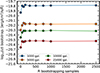 |
Fig. A.1. Uncertainties (at 1σ level) of the median stacked spectra as a function of number of bootstrap samples. Different curves and colours vary depending on the number of individual spectra in the stacking (1000, 5000, 10 000, 25 000 galaxies). |
Appendix B: Sample selection for stacking
In this section we identify the zprob threshold at a given flux limit that enables the selection of observationally defined samples for stacking, striking a balance between minimising contamination (𝒞) and maximising success rate (𝒮ℛ).
In Fig. B.1 we show the variation of the distribution of EWS-SFsim Hα fluxes with increasing zprob thresholds, to demonstrate which is the net effect of progressively increasing the zprob threshold on the flux distribution. The top panel refers to the flux threshold 2 × 10⁻¹⁷ erg s−1 cm−2, whereas the bottom one is for 2 × 10⁻¹⁶ erg s−1 cm−2. In the top panel, we observe that higher zprob cuts lead to net distributions at higher Hα fluxes, progressively reducing the completeness at fainter fluxes. The purple distribution represents the distribution corresponding to the benchmark sample (no cut in zprob). Then, as we progressively increase the zprob threshold, we are filtering out fainter galaxies from the selection, resulting in a brighter median Hα flux, and we expect to observe this effect also in the corresponding stacked spectra. This result demonstrates that our goal of probing fainter galaxy populations within the EWS through stacking is fundamentally constrained by the need to rigorously clean the sample of redshift contaminants. This process, whilst necessary, has the drawback of reducing the inclusion of the target population at fainter fluxes. As a result, attempting to push to deeper fluxes with stacking could become ineffective, as the selected sample is progressively reduced at fainter fluxes. In contrast, the bottom panel of Fig. B.1 shows that for the fiducial flux threshold of 2 × 10⁻¹⁶ erg s−1 cm−2, increasing the zprob cut has a minimal impact on the Hα distribution. Therefore, in this case we expect the quality of the stacked spectra across different zprob cuts to depend primarily on the influence of residual redshift contaminants that are not removed by the selection cuts.
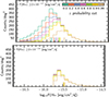 |
Fig. B.1. Distributions of true Hα flux for the mock EWS-SFsim sample. The top panel shows galaxies with true Hα flux F(Hα) ≥2 × 10⁻¹⁷ erg s−1 cm−2, whereas the bottom panel shows galaxies with F(Hα) ≥2 × 10⁻¹⁶ erg s−1 cm−2. |
We analysed how zprob thresholds and flux limits affect the success rate and contamination level in stacked spectra for the EWS-SFsim. Galaxies were selected within [zmin, zmax]=[1.52, 1.86], where strong emission lines from Hβ to Hα lie within the red grism’s wavelength range. This selection ensures uniform coverage of key spectral lines. For stacking, we tested combinations of the following parameters
-
zprob thresholds: 0, 0.2, 0.4, 0.6, 0.8, 0.9, 0.99.
-
Stellar mass (in bins of Δlog10M* = 0.5): [9, 9.5], [9.5, 10], [10, 10.5], [10.5, 11], [11, 11.5]. Note that we did not consider higher stellar masses due to the limited number of galaxies with M* > 1011.5 M⊙ in the 3 deg2 volume covered by our simulation.
-
Flux thresholds for the Hα line: 2 × 10⁻¹⁷ and 2 × 10⁻¹⁶ erg s−1 cm−2.
For each combination, a stacked spectrum was generated applying Eq. (6). Stacking was performed using SpectraPyle with the following process: individual spectra were shifted to z = 1.68 (the median redshift of the EWS-SFsim sample), scaled for cosmological flux, and re-projected onto a uniform 0.5 nm wavelength grid. Median fluxes were then extracted at each pixel, with uncertainties estimated via 350 bootstrap realizations. Key emission lines (Hα, [N II], [O III], Hβ) were deblended and measured in the stacked spectra using the SlineFit code.
Figure B.2 presents the success rate (𝒮ℛ) as a function of contamination (𝒞), colour-coded by the redshift probability threshold (zprob), for the EWS-SFsim. Top panels correspond to a flux limit of 2 × 10⁻¹⁷ erg s−1 cm−2; bottom panels show the fiducial case at 2 × 10⁻¹⁶ erg s−1 cm−2.
At the lowest flux limit, 𝒮ℛ remains below 37% in all stellar mass bins, declining to 12% in the lowest bin, regardless of the applied zprob cut. As anticipated from Fig. B.1, higher zprob thresholds exclude low-S/N galaxies, reducing 𝒞 but also removing intrinsically fainter Hα emitters and lowering 𝒮ℛ. This unfavourable trade-off makes this flux limit unsuitable for robust stacking: high-zprob cuts lead to biased samples dominated by bright emitters, while low-zprob cuts yield excessive contamination. Consequently, we do not recommend using a 2 × 10⁻¹⁷ erg s−1 cm−2 limit for stacking purposes.
In contrast, the fiducial 2 × 10⁻¹⁶ erg s−1 cm−2 sample shows improved performance. At zprob = 0, 𝒮ℛ exceeds 70% across all mass bins, albeit with a contamination of between 30-70%. Increasing zprob progressively lowers 𝒞 while preserving high 𝒮ℛ up to zprob = 0.9. For instance, in the [10, 10.5] bin, 𝒞 drops from 50% to 10% while maintaining 𝒮ℛ at roughly 80%. Beyond zprob = 0.9, the contamination continues to decrease, albeit more slowly, while the 𝒮ℛ also declines. We adopt zprob = 0.99 to balance contamination control and completeness, limiting contamination to below 5% while retaining a success rate of roughly 50–77%. Intermediate flux thresholds (5 × 10⁻¹⁷ and 1 × 10⁻¹⁶ erg s−1 cm−2) perform better than the lowest limit but fall short of the efficiency achieved at the fiducial value and are not discussed further.
In summary, we adopt a selection based on zprob ≥0.99 and a flux limit of 2 × 10⁻¹⁶ erg s−1 cm−2 in the main analysis. This combination ensures high completeness with minimal contamination, preserving the fidelity of stacked spectral measurements (see Sect. 6).
We applied the same framework to the EDS-SFsim sample, which benefits from deeper flux sensitivity and extended spectral coverage via the blue grism, enabling the analysis of a broader redshift interval (0.9 ≤ z ≤ 1.86). To minimise evolutionary effects, we divided the sample into three redshift bins: [0.9, 1.2], [1.2, 1.52], and [1.52, 1.86], with the latter overlapping the EWS-SFsim range. The selection optimization tests were conducted in this uppermost redshift bin.
We used the same grid of parameters as in the EWS-SFsim analysis, but extended the stellar mass range down to log10(M*/M⊙)∈[8.5, 9], enabled by the lower flux threshold of 5 × 10⁻¹⁷ erg s−1 cm−2. Figure B.3 summarises the results. The trends are qualitatively similar to the EWS-SFsim case but show substantially better performance: at 2 × 10⁻¹⁷ erg s−1 cm−2, 𝒞 remains below 18% across all zprob cuts, and 𝒮ℛ exceeds 80%. At 5 × 10⁻¹⁷ erg s−1 cm−2, success rates reach 90%. This robustness makes selecting a single criterion less critical.
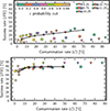 |
Fig. B.2. Success rate (𝒮ℛ) vs contamination rate (𝒞) for the mock EWS-SFsim, colour-coded by the applied redshift probability threshold (zprob). The top panel shows results for a flux threshold of 2 × 10⁻¹⁷erg s−1 cm−2, while the bottom panel corresponds to a higher threshold of 2 × 10⁻¹⁶erg s−1 cm−2. Different symbols represent galaxies in distinct stellar mass bins. As a reference, the black curves connect the points corresponding to the mass bin log10(M*/M⊙)∈[10, 10.5]. |
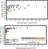 |
Fig. B.3. Success rate (𝒮ℛ) vs contamination rate (𝒞) for the mock EDS-SFsim, colour-coded by the applied redshift probability threshold (zprob). The top panel shows results for a flux threshold of 2 × 10⁻¹⁷erg s−1 cm−2, while the bottom panel corresponds to a higher threshold of 5 × 10⁻¹⁷erg s−1 cm−2. The layout is the same as in Fig. B.2. |
Nevertheless, to ensure consistency with the benchmark population, we adopt a flux limit of 2 × 10⁻¹⁷ erg s−1 cm−2 and a zprob threshold of 0.4 for the EDS-SFsim sample. This choice provides the best balance between completeness and contamination across stellar mass bins.
We caution, however, that although simulations remain robust down to 2 × 10⁻¹⁷ erg s−1 cm−2, actual galaxies with HE < 26 may fall below this sensitivity, potentially limiting redshift recovery in the real survey. As such, our contamination estimates may be slightly optimistic, and follow-up validation using real Euclid data will be essential.
In conclusion, based on the selection criteria, stacked spectra for the EDS-SFsim were generated with an Hα flux limit ≥2 × 10⁻¹⁷ erg s−1 cm−2 and a redshift probability threshold of zprob ≥ 0.4, whilst for the EWS-SFsim, stacked spectra were created with a stricter flux limit in Hα of ≥2 × 10⁻¹⁶ erg s−1 cm−2 and a redshift probability threshold of zprob ≥ 0.99.
Appendix C: Scaling relations for EDS-SFsim, in other redshift bins
In this appendix we present the scaling relations derived from the EDS-SFsim stacked spectra in the lower redshift bins 0.9 ≤ z ≤ 1.2 and 1.2 ≤ z ≤ 1.52. These results are qualitatively consistent with those discussed in Sect. 7 for the highest redshift bin (1.52 ≤ z ≤ 1.86). The emission line fluxes (Fig. C.2), measured from the stacked mock spectra shown in Fig. C.1, along with derived physical quantities such as attenuation, the star-formation rate–stellar mass relation (Fig. C.3), the BPT diagram (Fig. C.4), and gas-phase metallicity (Fig. C.5), exhibit the same overall behaviour, with only modest variations attributable to the cosmological evolution encoded in the MAMBO simulation. In particular, the fluxes of key emission lines (e.g. Hα, [O III], [N II]) measured from stacked spectra track the corresponding benchmark samples with comparable accuracy, and the main sequence relations maintain their characteristic shapes and slopes. We note slight differences in normalization and scatter that reflect the gradual evolution of galaxy properties over cosmic time, as expected from both simulations and observations. These differences remain well within the uncertainties and do not alter the qualitative conclusions drawn for the higher redshift bin.
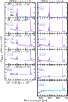 |
Fig. C.1. Stacked mean spectra for the mock EDS-SFsim galaxies used for the scientific predictions in this paper, for the redshift bins [0.9, 1.2] (left panels), and [1.2, 1.52] (right panels). The layout and notes are the same as in Fig. 13. |
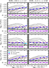 |
Fig. C.2. Emission line fluxes (in units of erg s−1 cm−2) measured on stacked mock spectra as a function of stellar mass for the EDS-SFsim selection corresponding to the redshift intervals 0.9 ≤ z ≤ 1.2 (left panels), and 1.2 ≤ z ≤ 1.52 (right panels). From top to bottom, panels show the fluxes of Hα, Hβ, [O III], and [N II] emission lines. Fluxes have been corrected for flux loss using the method by Cassata et al. (in preparation). The layout is the same as in Fig. 14. |
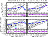 |
Fig. C.3. Attenuation–M* relation (top panels) and the SFR–M* relation (bottom panels) derived from the EDS-SFsim stacked mock spectra for the EDS-SFsim selection corresponding to the redshift intervals 0.9 ≤ z ≤ 1.2 (left panels), and 1.2 ≤ z ≤ 1.52 (right panels). The attenuation is measured using the Balmer decrement (Hα/Hβ ratio), while the SFR is calculated from the dust-corrected Hα luminosity, applying the Calzetti et al. (2000) extinction law and assuming case B recombination conditions (electron density of 100 cm−2 and 10 000 K. The panel layout follows the structure of Fig. 14. Shaded regions represent the 1σ uncertainties in the measured quantities. |
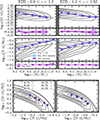 |
Fig. C.4. BPT diagram and corresponding stellar mass relations for the [O III]/Hβ and [N II]λ6584/Hα ratios based on the EDS-SFsim stacked mock spectra. The top and middle panels show the [O III]/Hβ–stellar mass (i.e. the MEx diagnostic diagram, Juneau et al. 2011), and [N II]λ6584/Hα–stellar mass relations, respectively, with measurements from the stacked spectra in different stellar mass bins. The bottom panel displays the BPT diagram with symbols representing the positions of the stacked spectra for various mass bins. The black contours in all panels represent the EDS-SFsim parent sample cut at HE ≤ 26, and the black dashed curves in the top and middle panels represent its median relations. |
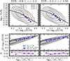 |
Fig. C.5. Top panels: O3N2 as a tracer of the gas-phase metallicity 12+log10(O/H) parameter, in the redshift bins [0.9, 1.2], and [1.2, 1.52]. The O3N2 values for stacked mock spectra in this study are calibrated using the Curti et al. (2017) relation. The layout of the panels is consistent with the bottom panel of Fig. 18. Bottom panels: Mass-metallicity relation (MZR), showing the dependence of gas-phase metallicity (inferred from O3N2) on stellar mass. The layout matches Fig. 14. |
All Figures
|
Fig. 1. Redshift coverage of prominent emission lines in the EWS and EDS spectra. For each emission line, the full coloured bar represents the redshift range where the line is detectable in the RGS for the EWS, whilst the dashed bar indicates the extended redshift coverage provided by the BGS in the EDS. |
| In the text | |
|
Fig. 2. Flowchart of the code SpectraPyle. The letter (d) indicates default options and parameters. |
| In the text | |
|
Fig. 3. True flux vs redshift for key emission lines in the mock EDS-SFsim (top) and EWS-SFsim (bottom) samples. Contours in dark green, light green, blue, orange, and red correspond to Paβ, Hα, [N II]λ6584, [O III], and Hβ, respectively, selected to span a broad redshift range and wavelength coverage. Each line’s redshift range reflects its detectability within the grism coverage. Contours from lighter to darker shades trace the 99th, 84th, 50th, 16th, and 1st percentiles of the distribution. Grey areas mark fluxes below the survey sensitivity limits. |
| In the text | |
|
Fig. 4. Example of a simulated spectrum from MAMBO of a galaxy at redshift z ∼ 1.6, stellar mass of log10(M*/M⊙) = 10.8, HE ∼ 21.1, SFR of 232.7 M⊙/yr, effective disk radius of |
| In the text | |
|
Fig. 5. Distribution of the continuum S/N per Å for the sample of simulated MAMBO spectra (see Sect. 4.1), providing a reference for typical input spectra quality. The black line represents the EWS MAMBO sample, selecting galaxies with HE < 24. The red and blue lines correspond to the EDS red and blue MAMBO samples, respectively, selecting galaxies at the survey limit of HE < 26. |
| In the text | |
|
Fig. 6. Measured redshift vs true redshift for the mock EWS-SFsim (top panel) and the EDS-SFsim (bottom panel). Bins are colour-coded according to the number counts per deg2. |
| In the text | |
|
Fig. 7. Left panel: Example of redshift contaminants due to [S III]λ9531 at 1752.7 nm mis-identified as Hα, yielding zmeas = 1.67 instead of ztrue = 0.836. Right panel: Median (in blue) and mean (in red) stack of 200 spectra (in grey) of galaxies where the [S III]λ9531 line was misinterpreted as Hα. Vertical dotted lines indicate the ‘true’ lines, while the coloured bands highlight the expected rest-frame positions of key optical emission lines at the wrong redshift of the stacked spectrum (Hβ, [O III], Hα, and [N II]). |
| In the text | |
|
Fig. 8. Left panel: Example where a random noise spike is misinterpreted as the Hα emission line, leading to an erroneous redshift measurement. Right panel: Median (in blue) and mean (in red) stacked spectrum of 500 spectra (in grey) of galaxies with misclassified redshift, illustrating the accumulation of these spurious noise spikes at notable lines positions. |
| In the text | |
|
Fig. 9. Distribution of measured Hα fluxes (corrected for flux loss following Cassata et al., in prep.) versus true Hα fluxes for the EDS-SFsim (top) and EWS-SFsim (bottom) simulated samples. Blue histograms show galaxies with accurate redshifts with |Δz|/(1 + z)≤0.003, red histograms indicate contaminants from mis-identified emission lines, and grey histograms represent contaminants from noise spikes. |
| In the text | |
|
Fig. 10. Stacked mean spectrum of simulated MAMBO galaxies from the EWS with stellar masses in the range 1010 M⊙ ≤ M* ≤ 1010.5 M⊙ and redshifts 1.52 ≤ z ≤ 1.86. The stacked is composed of a mixture of 2642 spectra, with contributions from galaxies with accurate redshifts (51%), as well as redshift contaminants arising from noise spikes (36%), [S III]λ9531 misclassified as Hα (8%), and [O III] misclassified as Hα (2%), plus minor contributions from other misclassified emission lines (∼5% in total). The plot includes the mean spectrum (red) and composite spectra at the 16th, 84th, 90th, 98th, and 99th percentiles (brown, orange, yellow, blue, and green, respectively). The contribution of individual galaxy spectra is shown in black. |
| In the text | |
|
Fig. 11. Simulated Hα emission line as a function of stellar mass for the EDS-SFsim selection is shown for the lowest redshift range: 0.9 ≤ zmeas ≤ 1.2. Top panels present the relation at the flux limit of F(Hα)≥2 × 10⁻¹⁷ erg s−1 cm−2 and with no cut in zprob, whilst the bottom panels present the improvement obtained with our fiducial selection that also includes a cut in redshift probability zprob ≥ 0.4. The left panels show the distributions of the different subsamples: the ℬℳ sample (grey points; Eq. (7)), the observationally selected galaxies with accurate redshifts (green points), and the redshift contaminants (red points). Note that the green and red points together constitute the observationally selected sample, as defined by the denominator of Eq. (6). Black and cyan contours and dashed lines show the ground-truth distributions for the full EDS parent sample (HE ≤ 26) and a subsample selected with F(Hα)≥2 × 10⁻¹⁷ erg s−1 cm−2, respectively. These contours serve as a reference to illustrate the intrinsic (ground-truth) distributions, allowing for a qualitative comparison with the observation-like measurements, and to highlight the intrinsic selection bias introduced by the flux limit, which would persist even without redshift measurement errors. The right panels show galaxy number densities per deg2 in bins of stellar mass and Hα flux, with 𝒮ℛ (top number) and 𝒞 (bottom number) indicated. Numbers are colour-coded: black-blue for reliable bins (𝒮ℛ > 45%, 𝒞 < 20%) and red and magenta for others. The numbers reported above each mass bin represent the 𝒮ℛ (top number) and 𝒞 (bottom number) for the entire mass bin. |
| In the text | |
|
Fig. 12. Simulated Hα emission line as a function of stellar mass for the EWS-SFsim selection. Top panels present the relation at the flux limit of F(Hα)≥2 × 10⁻¹⁶ erg s−1 cm−2 and with no cut in zprob, whilst the bottom panels present the improvement obtained with our fiducial selection that also includes also a cut in redshift probability zprob ≥ 0.99. The layout is the same as in Fig. 11, the only difference is that the black and cyan contours and dashed lines show the ground-truth distributions for the full EWS parent sample (HE ≤ 24) and a subsample selected with F(Hα) ≥ 2 × 10⁻¹⁶ erg s−1 cm−2, respectively. Note: in this case, the bias between the cut in magnitude only and the cut in magnitude and flux limit is larger than the EDS-SFsim one. Therefore, even with stacking, we are mapping scaling relations of galaxies with Hα flux above 2 × 10⁻¹⁶ erg s−1 cm−2. |
| In the text | |
|
Fig. 13. Stacked mean spectra for the mock galaxies used for the scientific predictions in this paper, for the redshift bin [1.52, 1.86]. The panels show stacked spectra divided by sample type and stellar mass bins: left panels show the EDS-SFsim, while right panels show the EWS-SFsim. Rows correspond to stellar mass bins of 0.5 dex, ranging from log10(M*/M⊙)≥8.5 to ≤11.5. Bins with fewer than 50 spectra are not shown or considered in the analysis. In each panel, cyan and magenta spectra represent the stacked spectra for the ℬℳ and observationally selected samples, respectively, with the numbers indicating the spectra counts. Note that the [O III]/[O III]λ4959 ratios of all stacks here are approximately 2.3, lower than the theoretical value of 3, due to an error in the simulated [O III]λ4959 emission line. Since the [O III] values are correct and [O III]λ4959 was not used in the analysis, the results remain unaffected. |
| In the text | |
|
Fig. 14. Emission line fluxes (in units of erg s−1 cm−2) measured on stacked spectra as a function of stellar mass for the EDS-SFsim selection corresponding to the redshift interval 1.52 ≤ z ≤ 1.86. From top to bottom, panels show the fluxes of Hα, Hβ, [O III], and [N II] emission lines. Fluxes have been corrected for flux loss using the method by Cassata et al. (in preparation). Magenta curves represent measurements from observationally selected galaxy stacks, whilst cyan circles correspond to benchmark (ℬℳ) stacks. The red dotted horizontal line in each panel indicates the flux limit of 2 × 10⁻¹⁷ erg s−1 cm−2 imposed on the EDS-SFsim. Shaded regions denote the 1σ uncertainty, whilst black contours and the dashed black line in each panel trace the ground-truth distribution and median relation of the parent EDS-SFsim sample (HE ≤ 26), respectively. The bottom insets in each panel show the difference (in dex) between the observational and benchmark flux measurements. |
| In the text | |
|
Fig. 15. Emission line fluxes measured on stacked mock spectra as a function of stellar mass for the EWS-SFsim selection. From top to bottom, panels display the fluxes of Hα, Hβ, [O III], and [N II] emission lines. The red dotted horizontal line in each panel indicates the flux limit of 2 × 10⁻¹⁶ erg s−1 cm−2 imposed on the Hα line. The layout of the panels is the same as in Fig. 14. |
| In the text | |
|
Fig. 16. Attenuation–M* relation (top panels) and the SFR–M* relation (bottom panels) derived from the EDS-SFsim stacked spectra. The attenuation is measured using the Balmer decrement (Hα/Hβ ratio), while the SFR is calculated from the dust-corrected Hα luminosity, applying the Calzetti et al. (2000) extinction law and assuming case B recombination conditions (electron density of 100 cm−2 and 10 000 K. The panel layout follows the structure of Fig. 14. Shaded regions represent the 1σ uncertainties in the measured quantities. |
| In the text | |
|
Fig. 17. Attenuation–M* relation (top panel) and the SFR–M* relation (bottom panel) derived from the EWS-SFsim stacked mock spectra. The attenuation is measured using the Balmer decrement (Hα/Hβ ratio), whilst the SFR is calculated from the dust-corrected Hα luminosity, applying the Calzetti et al. (2000) extinction law and assuming case B recombination conditions (electron density of 100 cm−2 and temperature of 10 000 K. The panel layout follows the structure of Fig. 14. Shaded regions represent the 1σ uncertainties in the measured quantities. |
| In the text | |
|
Fig. 18. BPT diagram and corresponding stellar mass relations for the [O III]/Hβ and [N II]λ6584/Hα ratios based on the EDS-SFsim stacked mock spectra. Top and middle panels show the [O III]/Hβ–stellar mass (i.e. the MEx diagnostic diagram, Juneau et al. 2011), and [N II]λ6584/Hα–stellar mass relations, respectively, with measurements from the stacked spectra in different stellar mass bins. The bottom panel displays the BPT diagram with symbols representing the positions of the stacked spectra for various mass bins. The black contours in all panels represent the EDS-SFsim parent sample cut at HE ≤ 26, and the black dashed curves in the top and middle panels represent its median relations. |
| In the text | |
|
Fig. 19. BPT diagram and corresponding stellar mass relations for the [O III]/Hβ and [N II]λ6584/Hα ratios based on the EWS-SFsim stacked mock spectra. Top and middle panels show the [O III]/Hβ-M* (i.e. the MEx diagnostic diagram, Juneau et al. 2011), and [N II]λ6584/Hα-M* relations, respectively, with measurements from the stacked spectra in different stellar mass bins. The bottom panel shows the BPT diagram with symbols representing the positions of the stacked spectra for various mass bins. The black contours in all panels represent the EWS-SFsim parent sample cut at HE ≤ 24, and the black dashed curves in the top and middle panels represent its median relations. |
| In the text | |
|
Fig. 20. Top panels: O3N2 as a tracer of the gas-phase metallicity 12+log10(O/H) parameter for the EDS-SFsim, in the redshift bin [1.52, 1.86]. The O3N2 values for stacked mock spectra in this study are calibrated using the Curti et al. (2017) relation. The layout of the panels is consistent with the bottom panel of Fig. 18. Bottom panels: Mass-metallicity relation (MZR), showing the dependence of gas-phase metallicity (inferred from O3N2) on stellar mass. The layout matches Fig. 14. |
| In the text | |
|
Fig. 21. Top panel: O3N2 as a tracer of the gas-phase metallicity 12+log10(O/H) parameter for the EWS-SFsim. The O3N2 values for stacked mock spectra in this study are calibrated using the Curti et al. (2017) relation. The layout of the panels is consistent with the bottom panel of Fig. 18. Bottom panel: Mass-metallicity relation (MZR), representing the dependence of gas-phase metallicity (inferred from O3N2) on stellar mass. The layout matches Fig. 14. |
| In the text | |
|
Fig. A.1. Uncertainties (at 1σ level) of the median stacked spectra as a function of number of bootstrap samples. Different curves and colours vary depending on the number of individual spectra in the stacking (1000, 5000, 10 000, 25 000 galaxies). |
| In the text | |
|
Fig. B.1. Distributions of true Hα flux for the mock EWS-SFsim sample. The top panel shows galaxies with true Hα flux F(Hα) ≥2 × 10⁻¹⁷ erg s−1 cm−2, whereas the bottom panel shows galaxies with F(Hα) ≥2 × 10⁻¹⁶ erg s−1 cm−2. |
| In the text | |
|
Fig. B.2. Success rate (𝒮ℛ) vs contamination rate (𝒞) for the mock EWS-SFsim, colour-coded by the applied redshift probability threshold (zprob). The top panel shows results for a flux threshold of 2 × 10⁻¹⁷erg s−1 cm−2, while the bottom panel corresponds to a higher threshold of 2 × 10⁻¹⁶erg s−1 cm−2. Different symbols represent galaxies in distinct stellar mass bins. As a reference, the black curves connect the points corresponding to the mass bin log10(M*/M⊙)∈[10, 10.5]. |
| In the text | |
|
Fig. B.3. Success rate (𝒮ℛ) vs contamination rate (𝒞) for the mock EDS-SFsim, colour-coded by the applied redshift probability threshold (zprob). The top panel shows results for a flux threshold of 2 × 10⁻¹⁷erg s−1 cm−2, while the bottom panel corresponds to a higher threshold of 5 × 10⁻¹⁷erg s−1 cm−2. The layout is the same as in Fig. B.2. |
| In the text | |
|
Fig. C.1. Stacked mean spectra for the mock EDS-SFsim galaxies used for the scientific predictions in this paper, for the redshift bins [0.9, 1.2] (left panels), and [1.2, 1.52] (right panels). The layout and notes are the same as in Fig. 13. |
| In the text | |
|
Fig. C.2. Emission line fluxes (in units of erg s−1 cm−2) measured on stacked mock spectra as a function of stellar mass for the EDS-SFsim selection corresponding to the redshift intervals 0.9 ≤ z ≤ 1.2 (left panels), and 1.2 ≤ z ≤ 1.52 (right panels). From top to bottom, panels show the fluxes of Hα, Hβ, [O III], and [N II] emission lines. Fluxes have been corrected for flux loss using the method by Cassata et al. (in preparation). The layout is the same as in Fig. 14. |
| In the text | |
|
Fig. C.3. Attenuation–M* relation (top panels) and the SFR–M* relation (bottom panels) derived from the EDS-SFsim stacked mock spectra for the EDS-SFsim selection corresponding to the redshift intervals 0.9 ≤ z ≤ 1.2 (left panels), and 1.2 ≤ z ≤ 1.52 (right panels). The attenuation is measured using the Balmer decrement (Hα/Hβ ratio), while the SFR is calculated from the dust-corrected Hα luminosity, applying the Calzetti et al. (2000) extinction law and assuming case B recombination conditions (electron density of 100 cm−2 and 10 000 K. The panel layout follows the structure of Fig. 14. Shaded regions represent the 1σ uncertainties in the measured quantities. |
| In the text | |
|
Fig. C.4. BPT diagram and corresponding stellar mass relations for the [O III]/Hβ and [N II]λ6584/Hα ratios based on the EDS-SFsim stacked mock spectra. The top and middle panels show the [O III]/Hβ–stellar mass (i.e. the MEx diagnostic diagram, Juneau et al. 2011), and [N II]λ6584/Hα–stellar mass relations, respectively, with measurements from the stacked spectra in different stellar mass bins. The bottom panel displays the BPT diagram with symbols representing the positions of the stacked spectra for various mass bins. The black contours in all panels represent the EDS-SFsim parent sample cut at HE ≤ 26, and the black dashed curves in the top and middle panels represent its median relations. |
| In the text | |
|
Fig. C.5. Top panels: O3N2 as a tracer of the gas-phase metallicity 12+log10(O/H) parameter, in the redshift bins [0.9, 1.2], and [1.2, 1.52]. The O3N2 values for stacked mock spectra in this study are calibrated using the Curti et al. (2017) relation. The layout of the panels is consistent with the bottom panel of Fig. 18. Bottom panels: Mass-metallicity relation (MZR), showing the dependence of gas-phase metallicity (inferred from O3N2) on stellar mass. The layout matches Fig. 14. |
| In the text | |
Current usage metrics show cumulative count of Article Views (full-text article views including HTML views, PDF and ePub downloads, according to the available data) and Abstracts Views on Vision4Press platform.
Data correspond to usage on the plateform after 2015. The current usage metrics is available 48-96 hours after online publication and is updated daily on week days.
Initial download of the metrics may take a while.