| Issue |
A&A
Volume 707, March 2026
|
|
|---|---|---|
| Article Number | A380 | |
| Number of page(s) | 43 | |
| Section | Extragalactic astronomy | |
| DOI | https://doi.org/10.1051/0004-6361/202554054 | |
| Published online | 20 March 2026 | |
QSO MUSEUM
III. The circumgalactic medium in the Lyα emission around 120 z ∼ 3 quasars covering the SDSS parameter space. Witnessing the instantaneous active galactic nucleus feedback on halo scales
1
Max-Planck-Institut für Astrophysik, Karl-Schwarzschild-Str 1, 85748 Garching bei München, Germany
2
Max-Planck-Institut für Astronomie, Königstuhl 17, 69117 Heidelberg, Germany
3
Interdisziplinäres Zentrum für Wissenschaftliches Rechnen, Universität Heidelberg, Im Neuenheimer Feld 205, D-69120 Heidelberg, Germany
4
Zentrum für Astronomie, Institut für Theoretische Astrophysik, Universität Heidelberg, Albert-Ueberle-Straße 2, D-69120 Heidelberg, Germany
5
International Gemini Observatory/NSF NOIRLab, 670 N A’ohoku Place, Hilo, Hawai’i 96720, USA
6
School of Mathematics, Statistics and Physics, Newcastle University, Newcastle upon Tyne NE1 7RU, UK
★ Corresponding author: This email address is being protected from spambots. You need JavaScript enabled to view it.
Received:
6
February
2025
Accepted:
27
November
2025
Abstract
Recent surveys have shown that z ≳ 2 quasars are surrounded by hydrogen Lyman-α (Lyα) glows with diverse emission levels and extents. These characteristics seem to depend on the activity of embedded quasars, on the number of active galactic nucleus (AGN) photons that are able to reach the halo gas or circumgalactic medium (CGM), and on the physical properties of the CGM. In this framework, we present VLT/MUSE snapshot observations (45 minutes/source) of 59 z ∼ 3 quasars extending the long-term QSO MUSEUM campaign to the fainter SDSS sources. The whole survey is homogeneously reduced and analyzed here and now targets 120 quasars with a median redshift z = 3.13 and bolometric luminosities, black hole masses, and Eddington ratios in the ranges 45.1 < log(Lbol/[erg s−1]) < 48.7, 7.9 < log(MBH/[M⊙]) < 10.3, and 0.01 < λEdd < 1.8. We detected extended Lyα emission in 110 of the 120 systems, with all the nondetections in the newly added fainter sample. The surface brightness of the CGM Lyα emission (SBLyα) increases with quasar luminosity. Stacking of the nondetections unveiled emission just below our individual field detection limit. Moreover, the Lyα line width increases in the central regions (projected radius R < 40 kpc or ∼40% Rvir) of the CGM around quasars with stronger radiation. The variation in surface brightness and the velocity dispersion as a function of quasar luminosity indicate that we witness the instantaneous AGN feedback in action on CGM scales. Assuming that all targeted quasars sit in halos of MDM ∼ 1012.5 M⊙ independent of luminosity, as suggested by clustering studies, we explain the trend in SBLyα naturally by a larger fraction of cool gas mass that is illuminated, which implies that brighter quasars have larger ionization cone opening angles. Similarly, brighter AGN seem to perturb the cool (T ∼ 104 K) gas more strongly. We show that QSO MUSEUM starts to have enough statistics to study this instantaneous AGN feedback while controlling for black hole properties (e.g., mass), which will be key to constraining AGN models.
Key words: galaxies: halos / galaxies: high-redshift / intergalactic medium / quasars: emission lines / quasars: general
© The Authors 2026
 Open Access article, published by EDP Sciences, under the terms of the Creative Commons Attribution License (https://creativecommons.org/licenses/by/4.0), which permits unrestricted use, distribution, and reproduction in any medium, provided the original work is properly cited.
This article is published in open access under the Subscribe to Open model.
Open access funding provided by Max Planck Society.
1. Introduction
A large fraction of the baryons in the Universe are thought to reside in regions between the interstellar medium of galaxies and the virial radius of their host dark matter halo. This material, currently referred to as the CGM (Tumlinson et al. 2017), has been determined to be multiphase, including cold (10–100 K; e.g., Emonts et al. 2016; Vidal-García et al. 2021; Emonts et al. 2023), cool (∼104 K; e.g., Werk et al. 2014; Wisotzki et al. 2016; Nateghi et al. 2024), and hot gas (> 105 K; e.g., Predehl et al. 2020; Di Mascolo et al. 2023; Zhang et al. 2024). The importance of the CGM in galaxy evolution has become clearer in the past two decades, and its phases are currently under intense scrutiny (Faucher-Giguère & Oh 2023). The CGM stores information on the complex interplay of several processes during galaxy formation and evolution that successively shape galaxies, including gas inflows from the larger scales of the intergalactic medium (e.g., Kereš et al. 2005; Decataldo et al. 2024), galactic or active galactic nucleus (AGN) winds/outflows (e.g., Springel et al. 2005; Stinson et al. 2006; Wright et al. 2024), radiation (e.g., Ciotti & Ostriker 1997; Obreja et al. 2019), and interactions with and gas stripping of satellite galaxies (e.g., Hopkins et al. 2006; Anglés-Alcázar et al. 2017).
The CGM of AGNs is the optimal case study to encompass all of the aforementioned processes. AGNs, more specifically, those identified by the observation of their broad emission lines, that is, quasars, are known to reside in relatively massive halos up to z ∼ 6 (MDM ∼ 1012.5 M⊙; White et al. 2012; Timlin et al. 2018; Farina et al. 2019; Fossati et al. 2021; de Beer et al. 2023; Costa 2024). This mass range is thought to be characterized by (i) overdense environments around these systems that might contribute to their growth through infall and mergers (e.g., Kauffmann & Haehnelt 2000), and (ii) several satellite galaxies, some of which have high star formation rates (SFR ≳ 100 M⊙ yr−1), as demonstrated by recent observations (e.g., Decarli et al. 2017; Fossati et al. 2021; Chen et al. 2021; Bischetti et al. 2021; Arrigoni Battaia et al. 2022; Nowotka et al. 2022; Arrigoni Battaia et al. 2023a). Quasar host galaxies are also more massive and more strongly star forming than typical galaxies at the same cosmic time (e.g., Walter et al. 2009; Pitchford et al. 2016; Molina et al. 2023), which implies that their CGM and environment need to provide enough material to sustain this activity.
Importantly, quasars (supermassive black holes (SMBHs) accreting material), have extreme luminosities that are expected to expel, enrich, and highly ionize the gas reservoir within the host and its surroundings. This process is known as AGN feedback (e.g., Fabian 2012; King & Pounds 2015). To reach their exceptional masses (MBH ∼ 108 − 1010 M⊙), SMBHs are expected to be fueled in different regimes, including major mergers of gas-rich galaxies, giving rise to the most extreme black hole growth and assembly (e.g., Ni et al. 2022), and self-regulated growth mostly at the center of their host galaxies in a cycle of accretion and feedback (e.g., Di Matteo et al. 2005). Quasars have been observed to be highly variable (e.g., MacLeod et al. 2012), with typical variability timescales of about 105 − 6 years (Schawinski et al. 2015; Eilers et al. 2017) and ages of 106 − 108 years (Martini 2004; Khrykin et al. 2021). The quasar shut-down phase is loosely constrained to 104 − 105 years based on the geometry and extent of a few quasar light echoes and the recombination timescale of narrow-line emission (e.g., Lintott et al. 2009; Schirmer et al. 2013; Davies et al. 2015). The effect of quasars on their surrounding reservoir and environment is therefore not only almost instantaneous, but also cumulative (e.g., Harrison & Ramos Almeida 2024).
The quasar number density, and therefore, their activity, is at its apex at z ∼ 2 (e.g., Shen et al. 2020). This is fortunate because the CGM of quasars at its peak activity can therefore be probed in absorption against bright background sources and directly in emission. Absorption-line studies of the CGM of hundreds of z ∼ 2 − 3 quasars revealed the cool (T ∼ 104 K), massive (M ∼ 1011 M⊙), and metal rich (Z ∼ 0.5 Z⊙) gas reservoirs as traced by optically thick absorbers, whose spatial distribution is highly anisotropic, likely due to quasar illumination mainly along our line of sight (e.g., Hennawi & Prochaska 2007; Prochaska et al. 2014; Lau et al. 2016). These studies have been able to provide information on the average properties of the CGM gas despite the sparseness of bright background quasars. On the other hand, detailed information on the morphology, physical properties, and kinematics of the CGM around individual quasars requires direct observations.
The direct detection of the CGM of z ∼ 2 − 3 quasars has been a long-sought goal since early predictions of the possible presence of extended glows of hydrogen Lyα emission around AGNs (Rees 1988; Haiman & Rees 2001), which are thought to be caused by the quasar illuminating its surrounding distribution of infalling gas. Several spectroscopic and narrow-band studies were successful in unveiling their CGM gas out to distances of < 50 kpc (e.g., Hu & Cowie 1987; Weidinger et al. 2005; Christensen et al. 2006; Hennawi & Prochaska 2013; Arrigoni Battaia et al. 2016), but were hampered by the shallow sensitivity of past instrumentation and by the lack of accurate quasar systemic redshifts to gather statistical samples of detections. Notwithstanding these difficulties, these pioneering works were able to (i) unveil the Lyα signal out to even ∼500 kpc for the most exceptional systems (Cantalupo et al. 2014; Hennawi et al. 2015), (ii) constrain in a photoionization scenario the cool gas that emits Lyα to be dense and metal enriched in some cases (Heckman et al. 1991b,a), (iii) show that the kinematics of the CGM are relatively quiescent, possibly dominated by infall (Weidinger et al. 2004), and (iv) start to investigate correlations between nebula and QSO properties (Christensen et al. 2006).
The development of integral field spectrographs, such as the Multi Unit Spectroscopic Explorer (MUSE, Bacon et al. 2010) at the Very Large Telescope (VLT) and the Keck Cosmic Web Imager (KCWI, Morrissey et al. 2018) at the Keck Observatory revolutionized this field of research by allowing us to map the CGM of 2 < z < 6 bright quasars with unprecedented surface brightness limits (SBLyα ∼ 10 − 18 erg s−1 cm−2 arcsec−2). It was therefore possible to uncover the large diversity of Lyα nebulae (sample of ∼100 at z ∼ 3) with sizes up to ∼100 kpc in only one hour of telescope time per object (Borisova et al. 2016; Farina et al. 2017; Arrigoni Battaia et al. 2018; Ginolfi et al. 2018; Cai et al. 2018; Arrigoni Battaia et al. 2019a,b; Farina et al. 2019; Cai et al. 2019; Travascio et al. 2020; Drake et al. 2020; Lau et al. 2022; González Lobos et al. 2023).
The origin of the extended Lyα emission is subject of debate, even though quasars can provide enough ionizing photons to keep the surrounding gas ionized. Important parameters are frequently not known, including the fraction of volume that is illuminated by each quasar, or the quasar ionization cone opening angle, the geometry of the host galaxy and its position with respect to the quasar ionization cones, and the presence of winds/ouftlows. Several mechanisms can act together, and, through their combination, produce the observed Lyα glow: recombination radiation following gas ionization by the quasar radiation (e.g., Cantalupo et al. 2005; Kollmeier et al. 2010; Costa et al. 2022), shocks (e.g., Mori et al. 2004), resonant scattering of Lyα photons from the quasar broad-line regions (BLRs, e.g., Cantalupo et al. 2014; Costa et al. 2022), and gravitational cooling radiation (e.g., Haiman et al. 2000; Dijkstra et al. 2006). Furthermore, Lyα photons produced on CGM scales might resonantly scatter and shape the nebulae morphology and the spectral shape of the Lyα emission (Costa et al. 2022). Overall, the aforementioned observational studies more frequently highlighted the importance of photoionization due to the quasar radiation followed by recombination in optically thin gas. In this framework, the Lyα SB scales as the product of the gas mass and density (SB ; Hennawi & Prochaska 2013). In this scenario, the observed Lyα SB implies densities of the cool gas of nH ≳ 1 cm−1 (Hennawi et al. 2015; Arrigoni Battaia et al. 2015b, 2019b), which are comparable to star-forming regions in the interstellar medium of galaxies. Moreover, extended He IIλ1640 and C IVλ1549 emission has been detected in some individual cases or using a stacking analysis of tens of systems (Arrigoni Battaia et al. 2018; Cantalupo et al. 2019; Guo et al. 2020; Travascio et al. 2020; Fossati et al. 2021; Lau et al. 2022; Sabhlok et al. 2024), indicating that the cool CGM of 2 < z < 6 quasars is metal enriched and ionized, but not illuminated by the quasar radiation throughout (Obreja et al. 2024).
Most of these studies focused on the CGM of the brightest quasars, but recent work by Mackenzie et al. (2021) targeted 12 z ∼ 3 quasars with MUSE that were selected to be fainter (−27.1 < Mi(z = 2) < − 23.8) than previous studies and detected Lyα nebulae in all of them. The Lyα nebulae of fainter quasars reported in that work were fainter and less extended on average than those around brighter systems, which indicates that the Lyα SB of the nebula and the quasar UV and Lyα luminosities are correlated. The authors discussed several possible explanations for the observed relation, but no clear observational evidence to distinguish among them. The possible explanations they discussed were (i) a dependence on the halo mass, with brighter quasars sitting in more massive halos; (ii) varying opening angles, with fainter quasars having smaller opening angles; (iii) a different dominant powering mechanism for extended emission around the brighter and fainter quasars, with resonant scattering dominating the emission around bright quasars and recombination dominating at the faint end; and (iv) unresolved inner regions of the nebulae or an unresolved component from the interstellar medium of the host galaxy seen in faint quasars.
In this framework, we report the continuation of the survey called Quasar Snapshot Observations with MUse: Search for Extended Ultraviolet eMission (QSO MUSEUM; Arrigoni Battaia et al. 2019a; Herwig et al. 2024). Arrigoni Battaia et al. (2019a) (hereafter QSO MUSEUM I) detected a diversity of Lyα nebulae around 61 bright quasars at z = 3.17 with MUSE. QSO MUSEUM I showed that (i) quasars with very similar bolometric luminosities can be surrounded by very different extended Lyα emission (in extent and SB level; see also Arrigoni Battaia et al. 2023b), (ii) the amplitudes of the motions traced by the Lyα emission are consistent with gravitational motions expected in dark matter halos that host z ∼ 3 quasars, (iii) the level of Lyα emission evolves around z ∼ 2 and z ∼ 3 quasars, and (iv) the nebulae are likely powered by a combination of photoionization and resonant scattering of Lyα photons. Herwig et al. (2024) (hereafter QSO MUSEUM II) focused on the CGM of physically associated quasar pairs at different projected distances (50 − 500 kpc) and found that of the detected Lyα nebulae, the most extended stretch in the direction of each pair, suggesting that the extended Lyα emission traces the direction of interactions (close pairs) or cosmic web filaments (distant pairs).
In this work (QSO MUSEUM III), we extend the sample presented in the QSO MUSEUM I survey to a total of 120 single quasar fields by targeting 59 fainter systems (−27 < Mi(z = 2) < − 24) at z = 3.1 with MUSE, making it the largest effort to date to map the CGM of quasars at z ∼ 3. With this large sample, we can now test the findings presented by Mackenzie et al. (2021) in addition to the link between SMBH properties, AGN feedback, and extended Lyα nebulae. This paper is organized as follows: In Section 2 we provide an overview of the sample selection and data reduction, Section 3 highlights our main observational findings (SB levels, luminosities, morphology, and kinematics), and in Section 4 we discuss the relation between nebular emission and quasar properties, the implications of the observations in light of the quasar variability, the powering mechanisms, and the physical CGM properties, and we propose a simple model to address the observed trends. We adopted a flat ΛCDM cosmology with H0 = 70 km s−1 Mpc−1, Ωm = 0.3, and ΩΛ = 0.7. The size measurements are listed in units of physical kiloparsec unless otherwise specified. In this cosmology, 1 arcsec corresponds to ∼7.5 kpc at the median redshift of the sample (z = 3.1).
2. Observations and data reduction
2.1. Sample selection
The QSO MUSEUM I survey targeted with MUSE 61 quasars covering a range of absolute i-band magnitudes normalized at z = 2 of −29.67 < Mi(z = 2) < − 27.03 and redshift 3.03 < z < 3.46. These quasars represent the brightest objects not targeted by the MUSE Guaranteed Time Observation (GTO) team (Borisova et al. 2016). In this work, we extend the survey by targeting 58 additional quasars covering a fainter range of magnitudes −27 < Mi(z = 2) < − 24. Additionally, we include the z = 3.4 quasar discovered around ID 31 in QSO MUSEUM I (see their Appendix C). This sample has been constructed from the public spectroscopic quasar catalog of the Sloan Digital Sky Survey / Baryon Oscillation Spectroscopic Survey (SDSS/BOSS) data release 14 (DR14) (Pâris et al. 2018), selecting objects as in QSO MUSEUM I, but now in a more limited redshift range 3 < z < 3.2 and with the condition of having 20 targets per unit magnitude Mi(z = 2) bin in the aforementioned range (see Table A.1). The redshift range is chosen to target the lowest redshift accessible by MUSE in Lyα emission (close to the quasars’ activity peak), and to avoid contamination from stronger and more frequent sky lines at longer wavelengths. Figure 1 shows the Mi(z = 2) distribution of the QSO MUSEUM I sample (dark green) and the 59 fainter quasars presented in this work (orange). This extended sample makes up the largest search to date for nebular emission around z ∼ 3 quasars (120 systems). Additionally, we show in the same figure, the similarly faint quasar sample from Mackenzie et al. (2021) (yellow) and the bright quasars targeted by Borisova et al. (2016) (light green).
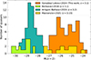 |
Fig. 1. Overview of the z ∼ 3 quasar samples with MUSE observations. The histograms of the absolute i-band magnitude (normalized at z = 2, following Ross et al. 2013) of the QSO MUSEUM III survey: 59 faint quasars from this study (orange), and 61 bright quasars from QSO MUSEUM I (dark green). For comparison, we show the 19 bright quasars from Borisova et al. (2016) (light green) and the 12 faint quasars from Mackenzie et al. (2021) (yellow). The median redshift of each sample is indicated in the legend. |
2.2. Physical properties of the targeted quasars
The physical properties of the targeted quasars are summarized in Figures 2, 3, and 4. The distribution of the peak Lyα luminosity density as a function of i-band absolute magnitude normalized at z = 2 (following Ross et al. 2013) of the bright and faint quasars is shown in Figure 2 with dark green and orange stars, respectively. The peak Lyα luminosity density is computed from the MUSE data cube by integrating a spectrum inside a 1.5″ radius aperture centered at the quasar location. In addition, we computed using the MUSE data cubes the values from the sample of 17 quasars targeted in Borisova et al. (2016) and 12 quasars from Mackenzie et al. (2021) and show them with light green and yellow triangles, respectively. For comparison, we computed the values from the SDSS DR17 (Abdurro’uf et al. 2022) 3.0 < z < 3.46 quasars. Figure 2 illustrates how the QSO MUSEUM survey now covers the parameter space of the SDSS quasar population. Specifically, the 120 quasars in QSO MUSEUM III encompass a wide range of quasar UV luminosities (six orders in Mi(z = 2)) and in peak Lyα quasar luminosity  (three orders).
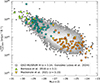 |
Fig. 2. Overview of the luminosity distribution of the observed z ∼ 3 quasars. The figure shows the quasar peak Lyα luminosity density as a function of absolute i-band magnitude normalized at z = 2 (Mi(z = 2), following Ross et al. 2013). The QSO MUSEUM III faint and bright quasars are shown with orange and dark green stars, respectively. The systems with no Lyα nebula detected are marked with a white dot (see Section 3.1). In addition, we show the location of the 17 brighter quasars targeted in Borisova et al. (2016) (light green triangles) and the 12 fainter objects from Mackenzie et al. (2021) (yellow triangles). The 2D number density of 3.0 < z < 3.46 quasars from SDSS DR17 (25 806 quasars, Abdurro’uf et al. 2022) is shown in logarithmic gray scale, white marking the highest densities. Section 2.2 explains how the luminosities are derived. |
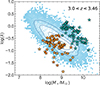 |
Fig. 3. Eddington ratio vs. black hole mass for the targeted sample. The data points for the QSO MUSEUM III sample (same symbols as in Figure 2) are compared with the values for SDSS quasars in the same redshift range (blue, 2-D number density histogram; Rakshit et al. 2020). The contours indicate the iso-proportions of the density at 0.2, 0.4, 0.68 and 0.95 levels, indicating that 20%, 40%, 68%, and 95% of the quasars are outside that contour, respectively. |
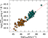 |
Fig. 4. Peak Lyα luminosity density vs. bolometric luminosity of the targeted quasars. The same symbols as Figure 2 indicate the bolometric luminosity of the quasar, which is is computed using the monochromatic luminosity Lλ(1350 Å) (see Appendix B). Systems where no Lyα nebulae were detected are marked with a white dot (see Section 3.2). The dashed red line represents a power law fit to the data of the form |

Further, for all the QSO MUSEUM III targeted quasars we estimated their black hole mass, bolometric luminosity and accretion rates. The first is calculated using the only available broad emission line observed for all the sample, C IV, and that allow us to derive single-epoch black hole masses using the Vestergaard & Peterson (2006) estimator,
![Mathematical equation: $$ \begin{aligned} \mathrm{{log}}M_{\rm {BH}}({\text{ C}}{\small {\uppercase {\text{ iv}}}}) = &\,\,\mathrm{{log}}\left\{ \left[\frac{\mathrm{{FWHM}({\text{ C}}{\small {\uppercase {\text{ iv}}}})}}{1000\, \mathrm{{km\, s}^{-1}}}\right]^{2} \left[ \frac{\lambda L_{\lambda }(1350\,\AA )}{10^{44}\, \mathrm{{erg\, s}^{-1}}} \right]^{0.53} \right\} \nonumber \\&\qquad +6.66, \end{aligned} $$](/articles/aa/full_html/2026/03/aa54054-25/aa54054-25-eq4.gif) (1)
(1)
where FWHM(C IV) is the width of the C IV line and Lλ1350 Å) is the monochromatic luminosity of the quasar at rest-frame 1350 Å. The values of FWHM(C IV) and Lλ(1350 Å) are obtained using the output from the fit to the quasar spectra using the public Python code PYQSOFIT1 (Guo et al. 2018) as described in Appendix B. The typical uncertainties on the estimate of the black hole masses (Equation 1) are about 0.5 dex.
With the MBH, we can compute the theoretical maximum luminosity for the case when radiation pressure and gravity are in equilibrium in a spherical geometry, that is, the Eddington luminosity (Eddington 1926) as
 (2)
(2)
where σT is the Thomson-scattering cross section, G is the gravitational constant, mp is the proton mass, and c is the speed of light. The Eddington luminosity is usually compared with the quasar bolometric luminosity (Lbol) to assess the activity and hence accretion rate of the SMBH. A so-called Eddington ratio is usually defined as
 (3)
(3)
We computed Lbol using the monochromatic luminosity Lλ(1350 Å) as done in Rakshit et al. (2020) using the bolometric correction factor given in Shen et al. (2011) and adapted from Richards et al. (2006),
 (4)
(4)
This estimate can have up to 0.3 dex of intrinsic uncertainty. The values computed of Lbol, together with MBH and λEdd are listed in Tables B.1 and B.2 together with their statistical uncertainties, which are much smaller than the aforementioned intrinsic uncertainties.
Figure 3 shows the Eddington ratio as a function of black hole mass for the QSO MUSEUM III sample with the same symbols as in Figure 2. Additionally, we show the number density for SDSS quasars in the same redshift range from Rakshit et al. (2020), who used almost the same fitting method to estimate such quantities (see details in Appendix B). Finally, we show the relation between the quasar peak Lyα luminosity density and their bolometric luminosity for the 120 quasars in Figure 4.
2.3. Observations
The observations were carried out with the MUSE instrument on the VLT 8.2m telescope YEPUN (UT4) over roughly 6.5 years (2014-2021). The data for the faint sample were taken as part of the European Southern Observatory (ESO) program 0106.A-0297(A) (PI: F. Arrigoni Battaia) in service mode on UT dates between 06-11-2020 and 10-03-2021 with good weather conditions (46.5% with clear sky, 46.5% with photometric sky, 7% with thin clouds; details in Table A.1)2 The observations were taken using the Wide Field Mode of MUSE, which covers a field of view of 1′×1′ with a 0.2″ pixel scale and a spectral range of 4750–9350 Å with a channel width of 1.25 Å and resolving power of R ∼ 1750 at 4984 Å (the expected Lyα wavelength at the median redshift of the sample). The observational strategy is the same as in QSO MUSEUM I, and consists of three exposures of 900 seconds each per field with a dither of < 5″ and 90 degree rotations with respect to each other. We summarize these observations in Table A.1. In particular, we report the absolute i-band magnitude normalized at z = 2 following Ross et al. (2013), the seeing at the expected Lyα wavelength (average of the 59 systems is 1.03″) the surface brightness limit within 1 arcsec2 and a 30 Å narrow band, and the Galactic v-band extinction (Av) from Schlegel et al. (1998). Similarly to Arrigoni Battaia et al. (2019a), we do not correct the fluxes and magnitudes by Galactic extinction. Using the reported Av and the relation from Cardelli et al. (1989), however, we derived a median flux increase of 11% at the observed Lyα wavelength of the sample. This factor does not affect our conclusions.
Additionally, we included in this work the MUSE observations of the 61 quasars from QSO MUSEUM I (see their Table 2). These data were taken as part of the ESO programmes 094.A-0585(A), 095.A-0615(A/B), and 096.A-0937(B) (PI: F. Arrigoni Battaia). The 120 systems are reduced and analyzed in this work using the exact same methods as described in Sections 2.4 and 2.5.
2.4. Data reduction
The data reduction for the whole sample comprised of 120 quasars was performed using the MUSE pipeline version 2.8.3 (Weilbacher et al. 2012, 2014, 2020) following the method described in Farina et al. (2019) consisting in subtraction of bias and dark field, flat field correction, wavelength calibration, illumination correction and standard star flux calibration. We removed the sky emission in each data cube using the Zurich Atmospheric Purge (ZAP; Soto et al. 2016) software. The MUSE pipeline underestimates the variance due to the noise correlation between pixels (Bacon et al. 2015), therefore we rescale each layer of the variance cubes to reflect the variance in the data cubes. The rescaled variance cubes are used to compute the surface brightness (SB) limits and errors in our estimations.
Following the method presented in González Lobos et al. (2023), the three3 reduced exposures of each target are median combined after masking artifacts due to the separation of the MUSE IFUs (consisting of ∼4% of the field of view). The final products are a final science data cube and a variance data cube obtained by taking into account propagation of errors during the combination. This final variance data cube is once again checked against the data by rescaling each layer to the variance computed in the corresponding combined science layer.
The average 2σ SB limit within 1 arcsec2 in a 30 Å narrow band (NB) at the observed Lyα wavelength of the sample is 2.2 × 10⁻¹⁸ erg s−1 arcsec−2 cm−2 (see Table A.1 for the individual SB limits). Per channel (1.25 Å) and within the same aperture and at the same wavelength, the data have an average 2σ SB limit of 4.3 × 10⁻¹⁹ erg s−1 arcsec−2 cm−2. These SB limits agree to those reported in Arrigoni Battaia et al. (2019a) despite the different analysis tools used in this work.
2.5. Revealing extended emission around quasars
The unresolved bright emission from a quasar can easily outshine the fainter emission from the surrounding CGM (e.g., Heckman et al. 1991b,a; Møller 2000). Therefore, we need to subtract the point spread function (PSF) of the quasar, as it has been frequently described in the literature (e.g., Borisova et al. 2016; Husemann et al. 2018; Farina et al. 2019; O’Sullivan et al. 2020; González Lobos et al. 2023), in order to characterize the extended CGM emission. In this work, we modified the Python routines developed and described in González Lobos et al. (2023) to reveal extended emission around quasars with different luminosities. For the bright objects we used parameters similar to those in Borisova et al. (2016) and Arrigoni Battaia et al. (2019a), while for the faint sample we used parameters similar to the ones used by Mackenzie et al. (2021).
Specifically, the PSF for faint quasars is constructed empirically using pseudo-NBs of 400 channels computed at each wavelength of the data cubes. This choice of pseudo-NB width is made to increase the signal to noise in the constructed PSF, similar to the 300 channels used in Mackenzie et al. (2021) and larger than the 150 channels used for brighter quasars (Borisova et al. 2016; Arrigoni Battaia et al. 2019a). Each pseudo-NB is normalized to the emission inside a region of 1 arcsec2 centered at the quasar coordinates, computed from the sigma clipped (3σ) average, and then subtracted from the data cube at the quasar position out to a radius of three times the seeing (see Table A.1).
Finally, we masked the 1 arcsec2 region located at the quasar position used for normalizing the pseudo-NB and exclude it from our analysis. Indeed this region is affected by PSF residuals (e.g., Borisova et al. 2016). We refer the reader to González Lobos et al. (2023) for more details on the algorithm.
After the PSF-subtraction, any extended emission could be still contaminated by the presence of continuum sources. We removed them using a median-filtering approach (e.g., Borisova et al. 2016) using the contsubfits function (with default parameters) within the ZAP4 (Soto et al. 2016) software. Such a method has been already used in other works targeting extended emission around quasars (Arrigoni Battaia et al. 2019b; Herwig et al. 2024).
3. Results
The final data cubes obtained in Section 2.5 contain only extended line emission, if detectable. In this study, we limit our investigation to the Lyα transition, and we defer the analysis of additional emission lines (He II, C IV) to subsequent works. We built Lyα SB maps, integrated spectra, velocity shift and velocity dispersion maps using such PSF- and continuum-subtracted data cubes, and present them in Figures 5, 6, A.1, A.2, 7 and 8, respectively. In the following sections, we describe how nebulae are detected and analyzed.
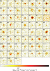 |
Fig. 5. QSO MUSEUM III atlas of the faint quasar Lyα nebulae. The Lyα SB maps around the 59 faint quasars after PSF and continuum subtraction (see Section 2.5), computed from 30 Å pseudo-NBs centered at the peak Lyα wavelength of the nebula. All images show maps with projected sizes of 20″ × 20″ (∼150 kpc × 150 kpc at the median redshift of the sample). In each map, a black crosshair indicates the location of the quasar and their ID number is indicated in top left corner. For systems with no detected nebula (Section 3.1), their ID number is indicated in color gray. The contours indicate levels of [2, 4, 10, 20, 50] times the Lyα SB limit within the pseudo-NB (Table A.1). |
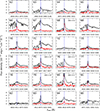 |
Fig. 6. One-dimensional spectrum covering the Lyα line for ID 62-85 in the new faint quasar sample. The ID of each quasar is shown in the top left corner of each panel. Each panel shows the spectrum integrated from the MUSE data cube inside a 1.5″ radius aperture centered at the quasar location (black line) and the integrated spectrum of each detected nebula integrated from the PSF- and continuum-subtracted data cubes within the 2σ isophotes from Figure 5 (red line), respectively. The wavelength of the peak of the Lyα emission of each quasar is indicated with a blue vertical line. The gray lines are the spectra integrated within a 1.5″ radius aperture from subtracted data cubes where we found no extended Lyα emission. We mask the 1″ × 1″ PSF normalization region when extracting a spectrum using the PSF- and continuum-subtracted data cubes. All the spectra are shown with the same y-axis scale and we indicate with a label in the top right corner of the panel if the quasar spectra has been rescaled by 0.6× or 0.3× for visualization. The reminder of the spectra (IDs 86 to 120) are shown in Figures A.1 and A.2. |
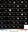 |
Fig. 7. Lyα velocity shift maps of the detected nebulae around z ∼ 3 faint quasars. The Lyα velocity shift map is computed from the first moment of the PSF- and continuum-subtracted data cubes within a ±FWHMLyα with respect to the wavelength of the peak of the Lyα emission of the nebula (Table A.2). The panels are shown using the same projected scale as Figure 5 (∼150 × 150 kpc) and a white crosshair indicates the location of the quasar. The ID of each system is shown at the top left corner of each panel. |
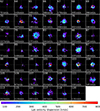 |
Fig. 8. Lyα velocity dispersion maps of the detected nebulae around z ∼ 3 faint quasars. The Lyα velocity dispersion map is computed from the second moment of the PSF- and continuum-subtracted datacubes within a ±FWHMLyα centered at the wavelength of the peak of the Lyα emission of the nebula (Table A.2). The panels are shown with the same projected scale as Figure 5 (∼150 × 150 kpc) and a white crosshair indicates the location of the quasar. The ID of each system and the average velocity dispersion within the mask are shown at the top and bottom left corner of each panel, respectively. The velocity dispersion of the faint quasars is on average lower than their bright counterparts (Figure C.6). |
3.1. Nebula detection
Using the PSF- and continuum subtracted data cubes, we extracted a spectrum inside a 1.5″ radius aperture centered at the quasar location, after masking the 1 arcsec2 normalization region (see Section 2.5). We used this spectrum to find Lyα emission by setting a 3σ detection threshold based on the variance associated to the spectrum within the same aperture, then finding the peak emission above this threshold. This method is more sensitive to circular nebulae, however we expect the nebular emission to be rather uniform within this region (see Section 3.3). We set the redshift of the detected nebulae using the wavelength of the peak Lyα emission from this method and list them in Table A.2, where nondetections are marked with dashed lines. We report the detection of 110 nebulae out of the 120 targeted quasars. All the nondetections occur in the fainter quasar sample, first presented in this work. We further check both the detections and nondetections by building SB maps from 30 Å pseudo-NB images and consider detected nebulae above 2σ as usually done in the literature (Section 3.2).
3.2. Lyman-α surface brightness maps and spectra
We used the redshift of the nebulae identified in Section 3.1 to build Lyα SB maps computed from 30 Å pseudo-NBs centered at the Lyα line. This wavelength range is chosen to allow comparison with previous studies. As in all former works (e.g., Borisova et al. 2016), we computed the residual background of each SB map after masking the location of continuum sources present in the original white image. We then subtracted the background level from each SB map.
The resulting SB maps for the 59 faint quasars and the 61 bright quasars are shown in Figures 5 and C.1, respectively, after smoothing using a 2D Box kernel of 3 pixels. For nondetections, we built the SB maps in a 30 Å pseudo-NB centered at the peak Lyα emission of the quasar spectra. The SB maps of Figure 5 correspond to ∼150 kpc × 150 kpc at the median redshift of the sample and show that the Lyα emission surrounding the fainter quasars appear dimmer and more compact than that observed around their bright quasar counterparts (Figure C.1), consistent with the findings of Mackenzie et al. (2021). As done in previous works, the detected nebulae are defined out to their 2σ isophote in the Lyα SB maps. We used this isophote to characterize the nebulae physical properties in Section 3.3. We note that there can be signal below this level but it would be at very low significance, and hence not quantified reliably.
For the 59 faint quasars, we integrated the spectra inside the 2σ isophotes and present the obtained one-dimensional spectra in Figures 6, A.1 and A.2 with red curves. For the nondetections, we show the spectrum integrated within a 1.5″ radius aperture in gray. The quasar spectra within a 1.5″ radius aperture are shown in black for comparison. The dashed blue line represents the wavelength of the peak Lyα emission of the quasar. In most cases, the Lyα emission of the detected nebulae resembles those of their associated quasars, even though the former is narrower, i.e, with similar absorption features and small shifts in wavelength compared to the Lyα line of the quasar. Moreover, some systems display absorption features in the quasar and nebula spectra at the same wavelength (e.g., ID 87, 96, 103, and 113), which could arise due to Lyα radiative transfer effects, outflows or dense material in front of the system (e.g., van Ojik et al. 1997; Gronke et al. 2015; Cai et al. 2018; Arrigoni Battaia et al. 2019b). The detailed modeling of these individual features is not the focus of this paper, however, and we defer their interpretation for future research. Finally, there are cases (e.g., ID 71, 73, 81, and 92) in which the Lyα emission occurs at wavelengths corresponding to absorption in the quasar spectrum. This result is similar to what has been found in the smaller sample studied in Mackenzie et al. (2021). The resulting spectra for the 61 bright quasars from the QSO MUSEUM I sample are presented in Figures C.2, C.3 and C.4 of Appendix C, and shows that our analysis is consistent with that work.
3.3. Nebulae morphologies, areas, integrated luminosities, and kinematics
We characterized the extended Lyα emission surrounding each quasar by integrating its Lyα luminosity, area within the 2σ isophote, morphology, velocity shift with respect to the quasar Lyα line and linewidth, which we summarize in Table A.2. Additionally, we obtained the spatial kinematics of the nebulae using the first and second moment maps which are presented in Figures 7 and 8.
First, we characterized the Lyα line spectra integrated inside the 2σ isophotes by fitting a Gaussian function, from which we computed the centroid wavelength and full width at half maximum (FWHM). We estimated the total Lyα luminosity of the nebulae by integrating the spectra within a wavelength range of ±FWHM (±2.355σ) centered on the Lyα line. This choice of wavelength range is selected so that we are considering most of the flux distribution into the calculation of the luminosity while excluding the noisiest part. The centroid of the Gaussian fit is used to compute the velocity shift of the nebula with respect to the peak Lyα emission of the quasar. All these quantities are also listed in Table A.2. We set an upper limit of 14 Å for the standard deviation when performing the Gaussian fit in some nebulae that show multiple components and/or absorption features in their integrated spectrum (see Table C.1 and Figures C.2, C.3 and C.4), therefore focusing the fit on the brightest component.
We also note that a Gaussian function is, in general, not a good representation of the Lyα line profile due to absorption features and possible radiative transfer effects affecting the propagation of Lyα photons. Therefore, we computed, for comparison, the first and second moment of the Lyα flux distribution to estimate the line centroid and linewidth within the ±FWHM range obtained from the Gaussian fit above. We found good agreement within uncertainties between the estimates from the Gaussian fit and flux weighted moments of the Lyα line flux distribution. We list in Table A.2 the flux weighted first moment of the line in terms of the velocity shift with respect to the quasar peak Lyα wavelength and the linewidth obtained from the second moment of the flux distribution.
In order to describe the kinematics of the observed nebulae, we computed the velocity shift and velocity dispersion maps shown in Figures 7 and 8 for the faint quasars and Figures C.5 and C.6 for the bright quasars. These maps are computed using the first and second moment of data cubes constructed within the ±FWHM range obtained from the Gaussian fit and centered at the peak Lyα wavelength of the nebulae. The calculation of the moment maps is restricted only to regions with a signal-to-noise ratio S/N > 3 in the respective SB maps obtained using a 30 Å pseudo-NB from the aforementioned data cubes, after applying a spatial smoothing with a Gaussian kernel of 0.5″. This spatial S/N > 3 mask is applied to the PSF- and continuum- subtracted cubes before computing the first and second moment maps5. The velocities are computed relative to the wavelength of the peak of each extended Lyα emission spectra.
The velocity shift maps of the faint sample (Figure 7) are complex and diverse, with some nebulae presenting velocity components that roughly span the range −200 km s−1 to +200 km s−1 with respect to the peak Lyα of the nebula (e.g., ID 66, 73, 96). Other nebulae appear to have more quiescent kinematics with velocity variations smaller than 100 km s−1 from the Lyα (e.g., ID 68, 80). On the other hand, the velocity shift maps of the bright sample (Figure C.5) display similar variety of complex velocity structures, with both quiescent and disturbed features in their nebulae. In particular, the largest velocity gradients for the bright quasars span a larger range than the faint nebulae of up to ∼600 km s−1 across the peak Lyα wavelength.
Most of the velocity dispersion maps of the faint quasars nebulae (Figure 8) show quiescent kinematics with velocity dispersions around 100 − 200 km s−1 and a tendency to increase up to 300 − 400 km s−1 toward the location of the quasar. On the other hand, the bright quasar nebulae (Figure C.6) have on average larger velocity dispersions ∼300 km s−1 and a similar tendency to increase up to 500 − 600 km s−1 toward the center. For both samples we see some cases where the velocity dispersion quickly increases to much higher values (800 − 1000 km s−1) at the center (radius smaller than ∼25 kpc). We further explore these findings in Section 3.4. Finally, we test how the velocity dispersion maps would change when decreasing the integrated S/N of the line emission in Appendix D. In summary, since the velocity range used to compute the second moment map is given by the integrated Lyα line Gaussian fit, then at a lower S/N there is a higher chance of fitting a broad linewidth. We show in Appendix D that S/N > 3 is a robust choice, which would give good results especially toward the centers of the maps.
The Lyα SB maps in Figures 5 and C.1 display a wide variety of morphologies, with some nebulae appearing centrally concentrated around the quasar position (e.g., ID 1, 39, 68, 80 among others), some seem to appear lopsided toward one direction from the quasar (e.g., ID 11, 36, 66, 109, 112) and finally some cases show large scale coherent structures (e.g., ID 13, 50, 56, 96). The strength of these effects could have an origin on the different powering mechanisms of extended Lyα nebulae, such as photoionization due to anisotropic quasar radiation (e.g, Obreja et al. 2024) or Lyα photons propagation (e.g, Costa et al. 2022). Moreover, the origin could be related to the gas distribution around each system (e.g., Cai et al. 2019) or viewing angle (e.g, Costa et al. 2022). Finally, the environment or presence of companions could affect the observed Lyα nebulae morphology (see e.g., Arrigoni Battaia et al. 2022; González Lobos et al. 2023; Herwig et al. 2024). We further discuss these scenarios in Section 4 and here we attempt to quantify the observed nebulae morphologies using two different measurements.
First, we quantify the asymmetry of the SB maps as previously done in the literature (e.g., Arrigoni Battaia et al. 2019a; Herwig et al. 2024), defined as the ratio of the semi-minor and semi-major axis within the 2σ isophotes used to describe the area of the detected nebulae (Tables A.2 and C.1). The ratio can be obtained as
 (5)
(5)
where Q and U are the stokes parameters computed from the flux weighted second order moments of the image following Equation 1 in Arrigoni Battaia et al. (2019a) within the 2σ isophote. The value of α corresponds to the aspect ratio of the isophote, with α = 1 representing a perfectly circular distribution. The top panel of Figure 9 shows the resulting α as a function of integrated Lyα nebula luminosity (Tables A.2 and C.1) within the same isophote for the faint and bright quasars with orange and dark green circles, respectively. Most (90%) of the observed nebulae have values of α ≳ 0.6, that is, the nebulae tend to be rounder. The median value of α estimated for the bright sample (dot-dashed green line) is also consistent with the value presented in QSO MUSEUM I (α = 0.77), considering the different data reduction and analysis used in this work. Similarly, we show that the α reported in the faint quasar sample from Mackenzie et al. (2021) (dotted gray line) appears to be consistent with the faint quasars presented in this work (dot-dashed orange line). Additionally, the median α of the faint sample is smaller than that of the bright quasars, indicating that faint quasars present slightly more elongated nebulae. To further test this, we estimated the average error in the calculation of α of the sample following the method presented in Herwig et al. (2024), who randomized the centroid coordinates in the flux weighted second moments in Equation 1 of Arrigoni Battaia et al. (2019a) and assumed the uncertainty is dominated by the seeing. This exercise results in a mean uncertainty of Δα = 0.05 which is comparable to the difference between the two median values of the bright and faint samples, therefore we cannot determine whether such a difference is significant. Further, we measured the Spearman rank correlation coefficient between α and LLyα;neb and obtain 0.19 with a p-value of 0.062, indicating a weak positive correlation that has low statistical significance. The same test between α and bolometric luminosities gives a similar result as expected due to the correlation between Lbol and LLyα;neb. Therefore, we infer that there is not a dependence between the elongation and luminosity of the nebulae or quasars. The lower median α estimated for the faint sample is also likely due to five of the dimmest nebulae (Lneb < 1043 erg s−1) studied here being associated with values representing more asymmetric or lopsided nebulae (α < 0.6). For comparison, we show the data-points of Lyα nebulae around associated projected quasar pairs from QSO MUSEUM II (dashed red line). Those systems present the lowest median α, which can be explained by the elongated morphology tracing the direction connecting the pairs. Summarizing, we find that there is no clear indication of a trend between α and LLyα;neb, which is also reported in those three works we compared to.
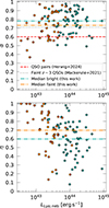 |
Fig. 9. Level of elongation (α) and lopsidedness (η) of the observed extended Lyα emission around quasars. In both panels, the orange and dark green points indicate the faint and bright sample of QSO MUSEUM III, respectively. The median values of the faint and bright samples are indicated with dot-dashed lines of the same colors. Top: Elongation α computed from the Stokes parameters (see Section 3.3) within the 2σ isophote of the detected nebulae as a function of nebula Lyα luminosity. Larger values of α indicate a rounder morphology. Additionally, we show the median values of α reported in the faint z ∼ 3 quasar sample from Mackenzie et al. (2021) and quasar pairs from QSO MUSEUM II with a gray dotted and dashed red line, respectively. Bottom: Nebula lopsidedness η as presented in Arrigoni Battaia et al. (2023b) and described in the text. High values correspond to all emission within the 2σ isophote being on one side of the quasar. |
In addition, we used the same 2σ isophotes to compute the asymmetry as done in Arrigoni Battaia et al. (2023b). In that work, the authors describe the asymmetry based on the ratio of areas  . Where
  and
and  are computed as the maximum and minimum area on both sides of the direction that crosses the quasar position and which maximizes the difference between the two covered areas. In this case, η represents the level of lopsidedness of the nebulae, that is, a value of η = 1 corresponds to all of the emission being on one side of the quasar. We plot η as a function of nebula luminosity within the 2σ isophote in the bottom panel of Figure 9 using the same symbols as the left panel. This figure shows that the dimmest nebulae appear more lopsided with respect to brighter nebulae. This is similar to the results found in Arrigoni Battaia et al. (2023b), where at a fixed SB threshold the smallest and dimmest nebulae appear more lopsided. Here, we did not use a fixed SB cut, but the systems studied here are found to lie close to the luminosity-area relation presented in that work for a common observed SB threshold corresponding to 2.46 × 10⁻¹⁷ erg s−1 cm−2 arcsec−2 at z = 2.0412 (see their Table 1). Likewise, we computed the Spearman rank correlation coefficient between η and LLyα; neb and find −0.29 with a p-value of 0.01 indicating a weak negative correlation. Particularly, we report that the systems with α < 0.5 and η ∼ 1 correspond to ID 62, 81 and 99 which have very low signal to noise and their emission on the SB maps appear irregular. For these systems the constructed 2σ isophote lies on one side of the quasar, which is a consequence of their clumpy morphology due to low SB levels. On the other hand, some bright systems appear lopsided and this could be an indication of larger scale structures. There is no clear trend between η and the nebula Lyα luminosity for nebulae around bright quasars, however.
By combining the information in both panels, we observe that most of the nebulae tend to have a circular morphology, but their emission tends to be preferentially toward one side of the quasar, that is, the nebulae emission is asymmetric with respect to the quasar position. The values of η span from centered to lopsided nebulae, however, and there is no discernible strong trend in relation to nebula luminosity or α. Finally, we note that the values of α and η are sensitive to the SB limit of each observation. This effect is particularly important for fainter nebulae, for which it is possible that the morphology would change if their fainter outskirts could be detected. We briefly discuss the possible implications of these observations in Section 4.3.
3.4. Radial profiles of the surface brightness and velocity dispersion
We have shown that the nebulae uncovered in this work are characterized by a diversity of morphologies, luminosities and kinematics. In this section, we quantify those differences by building radial profiles using the SB maps of Figures 5 and C.1 and the velocity dispersion maps of Figures 8 and C.6. The Lyα SB radial profiles are computed by averaging the maps inside annuli with logarithmically increasing radii centered at the quasar position, then corrected by cosmological dimming, as usually done in the literature (Arrigoni Battaia et al. 2019a; González Lobos et al. 2023). We extracted the SB radial profiles for all systems and compute the median profile for the faint and bright sample and show them in the top left panel of Figure 10 with orange and blue triangles, respectively. These profiles are plotted only out to the last radius where they exceed the 2σ detection limit of the stack, and the shaded areas represent their mean uncertainty. The profile shapes for the faint and bright samples are strikingly similar, however the SB normalization factor of the bright sample is about 6 times larger than the faint. The median values of each AGN property within the faint and bright sample bins are shown in the legend of Figure 11 and indicate a correlation between AGN luminosity and Lyα nebula SB. For comparison, we show the median profile of 12 similarly faint z ∼ 3 quasars from Mackenzie et al. (2021) (yellow line), and the analysis of the bright sample in QSO MUSEUM I (purple line). The agreement between our analysis and those in previous studies further substantiates the validity of our approach.
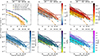 |
Fig. 10. Lyα SB radial profiles of the QSO MUSEUM III nebulae. The profiles of the detected nebulae are computed by averaging the Lyα SB maps of Figures 5 and C.1 inside annuli with logarithmically increasing radius centered at the quasar location, after masking the 1″ × 1″ normalization region. We cut the profiles when they reach values below the 2σ SB limit within the corresponding radial bin, and only plot profiles that have at least two data-points satisfying this criteria (108/110 profiles). The Lyα SB corrected by cosmological dimming is shown as a function of physical (bottom axis) and comoving (top axis) projected distances. Top left: Median profiles of the faint and bright sample (orange and green triangles) and stacked nondetections (gray). Additionally, the median profiles from Mackenzie et al. (2021) and Arrigoni Battaia et al. (2019a) are shown with a yellow and purple line, respectively. Top middle: Color-coded profiles according to the quasar absolute i-band magnitude normalized to z = 2. Top right: Color-coded profiles according to the peak of the Lyα luminosity density of the quasar. Bottom left: Color-coded profiles according to the bolometric luminosity of the quasar, computed from the monochromatic luminosity at 1350 Å (Appendix B). Bottom middle: Color-coded profiles according to their quasar black hole mass (Appendix B). Bottom right: Color-coded profiles according to their quasar Eddington ratio (Appendix B). |
Additionally, we construct a stacked SB map for the ten nondetections by median combining 30 Å pseudo-NB images centered at the wavelength of the peak of the quasar Lyα emission. This decision is based on the frequent observation that Lyα nebulae peak emission occurs at a similar wavelength of the quasar Lyα peak emission (Arrigoni Battaia et al. 2019a; Cai et al. 2019 and Section 4.3). We similarly propagate the associated variances to obtain errors. The stacked map shows a clear detection of which we show its SB profile in the top left panel of Figure 10 with gray circles and shaded area as the mean uncertainty. This SB profile is at the low end of all the observed individual nebulae and bolometric luminosities, confirming that these sources are just below our detection limit for individual systems and are three times dimmer than the median profile of the faint sample. Additionally, the nondetections have a median bolometric luminosity which is 1.3 times lower than the faint sample.
Further, the remaining panels in Figure 10 illustrate the individual Lyα SB profiles, which are color-coded according to their quasar properties: the absolute i-band magnitude normalized at z = 2 (top middle), the peak Lyα luminosity density of the quasar (top right), the bolometric luminosity of the quasar (bottom left), the black hole mass of the quasar (bottom middle), and Eddington ratio (bottom right). Each profile is cut when it reaches a value below the 2σ SB limit within a radial bin. We only show profiles with more than two data points, which result in a total of 108 profiles. The profiles span almost 2 orders of magnitude in their SB level and their shapes are similar across the whole sample. We further study the shape of the SB profiles by fitting a power and exponential function in Section 4.1. Figure 10 confirms – with 4× more systems – the correlation between quasar Lyα and UV luminosities and Lyα SB of the nebulae, also found in Mackenzie et al. (2021). In general, the profiles of nebulae around the faint sample have Lyα SB about one order of magnitude lower than the nebulae around bright quasars. The extended Lyα around the bright quasars is also detected out to projected distances of ∼100 kpc, while for the faint quasars, the Lyα is detected mostly out to 90 kpc. Additionally, the SB profile normalization factor increases as the peak Lyα luminosity and bolometric luminosity of the quasar increase. Such trend is not as clearly apparent with the absolute magnitude, as the profiles present larger Lyα SB scatter at a fixed quasar magnitude. Similarly, the black hole masses show scatter across the range of Lyα SB. Finally, there is a tendency for the brighter nebulae to also present the more extreme Eddington ratios, suggesting a potential link between nebula SB and AGN accretion rate.
In addition, we present in Figure 11 radial profiles that were constructed similarly to the SB profiles, but using the velocity dispersion maps of Figures 8 and C.6. These profiles are computed by averaging inside each annuli only where there is velocity dispersion data (within the S/N > 3 mask of Figures 8 and C.6). We overlay in the figure the spectral resolution limit of MUSE at the median Lyα wavelength (σ = 72 km s−1) with a shaded gray region. Note that the profiles approach this limit as the distance to the center increases, indicating that we need higher spectral resolution to resolve the lines at such distances. The velocity dispersion profiles tend to increase toward the quasar position, however. We color-coded the profiles by their quasar properties such as the peak Lyα luminosity density of the quasar (top left), the bolometric luminosity of the quasar (top right), the black hole mass (bottom left) and Eddington ratio (bottom right). We see a wide range of velocity dispersions, ranging from ∼100 km s−1 up to ∼1000 km s−1 within the innermost regions of the CGM of the targeted quasars (∼12 kpc). This scatter decreases to about 300 km s−1 as the projected distance increases (∼40 kpc), due to the steep decrease on the velocity dispersion of the nebulae around the brightest quasars. The median velocity dispersion profile for the faint and bright quasar sample shown in Figure 11 with thicker lines indicates that the velocity dispersion of bright quasar nebulae are about three times larger than fainter quasars at ∼12 kpc and only two times larger at ∼20 kpc. If we compare the velocity dispersion radial profiles to properties such as black hole masses and Eddington ratios we observe a similar behavior but less significant, probably because of the larger scatter of these properties across the range of luminosities probed with our sample.
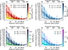 |
Fig. 11. Individual radial profiles of the Lyα velocity dispersion of the QSO MUSEUM III nebulae. Each profile is computed by averaging the Lyα velocity dispersion maps from Figures 8 and C.6 inside the S/N > 3 mask, using the same annuli as the profiles from Figure 10. Top left: The profiles are color-coded by the peak Lyα luminosity density of the quasar. Top right: The profiles are color-coded by the bolometric luminosity of the quasar. Bottom left: The profiles are color-coded by the black hole mass of the quasar. Bottom right: The profiles are color-coded by the Eddington ratio of the quasar. Additionally, we show in each panel the median velocity dispersion profile of the faint and bright samples, color-coded by each property with the median value of each bin indicated at the top right corner of the panel. In each panel, values below the MUSE spectral resolution limit (σ = 72 km s−1) are shown with a dashed gray area. |
4. Discussion
By targeting 59 additional faint (−27 < Mi(z = 2)−24) z ∼ 3 quasars, this work extends the current catalog of known Lyα nebulae by 49 additional detections, covering two orders of magnitude fainter systems than the bolometric luminosities studied in the QSO MUSEUM I survey (see Figure 4), and representing a factor of 4× more nebulae than are currently available at these quasar luminosities. This extended dynamic range allows us, for the first time with sufficient statistics, to study the CGM of quasars in emission across the faint and bright ends of the known z ∼ 3 quasar population (Figure 2), and link it to their AGN properties in addition to the physical mechanisms driving the emission.
4.1. Radial profiles of the stacked surface brightness and velocity dispersion
We design figures that summarize the main results on how the properties of quasar nebulae scale with quasar properties. The left panel of Figure 12 shows the bolometric luminosity as a function of black hole mass of the 110 quasars with detections in a log-log plot, color-coded by the peak Lyα luminosity density of the quasars. In this plot, quasars with similar Eddington ratios follow dashed gray diagonal lines. In the lower right corner of the same panel, we indicate with black error bars the intrinsic uncertainty of the log(MBH/M⊙) and log(Lbol/L⊙) estimators (Section 2.2), which correspond to 0.5 and 0.3 dex, respectively. We discuss the effect of these uncertainties further in Section 4.1.1. Additionally in this figure, the size of the symbols is proportional to the ratio of the total luminosity of the Lyα nebula and its area in kpc2 within their 2σ isophote, basically tracing the average Lyα SB of the nebula. This plot illustrates both the correlation between the quasar Lyα luminosity and their bolometric luminosity (see also Figure 4), and the increase in Lyα SB for brighter systems also seen in the Lyα SB profiles of Figure 10. Additionally, we show the same properties in the right panel of Figure 12, but color-coded by the mean velocity dispersion measured in the second moment maps of Figures 8 and C.6. The nebulae have a tendency to present larger average velocity dispersions with increasing bolometric luminosity (and hence also peak Lyα quasar luminosity), which was also observed in the velocity dispersion radial profiles of Figure 11. Therefore, the nebulae become brighter and potentially more turbulent with increasing bolometric luminosity at fixed black hole mass, or in other words with increasing Eddington ratios. In this section we explore the main drivers of these tendencies and the implications of these observations.
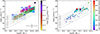 |
Fig. 12. Comparison of observed quasar properties with the nebulae properties. We show for each detected nebulae, their quasar bolometric luminosity as a function of black hole mass. The size of each point is proportional to the integrated Lyα luminosity of the nebula divided by the total nebula area in kpc2, with larger symbols having larger ratios. Different values of constant Eddington ratios (λEdd) are shown with dashed gray lines. Left: The points are color-coded by the peak Lyα luminosity density of each quasar (Table C.1). The black error bars in the lower right corner indicate the intrinsic uncertainty of the MBH and Lbol estimators (see Section 2.2). Right: The points are color-coded by the mean velocity dispersion shown in the maps of Figures 8 and C.6. Additionally, we overlay in the left panel the bins covering different quasar properties described in Section 4.1. |
4.1.1. Stacking data by AGN properties
We explore the principal factors responsible for the emergence of these trends by computing the median Lyα SB profiles using several bins encompassing different quasar properties. Stacking is done by first rebinning the profiles and their uncertainties into a common grid of projected comoving distances using a cubic spline interpolation, then we compute the median value at each radial bin. Since the stacking procedure decreases the noise potentially revealing fainter emission than in individual profiles, we also include in the stack the data points falling below the 2σ Lyα SB limit of each individual profile. We compute the mean uncertainty of each stacked radial bin by propagating their variances. Similarly, we rescaled the 2σ Lyα SB limit in the stacked bins and used it to cut the stacked profile at the radial distance at which it falls below the 2σ detection limit.
First, we built equally spaced bins of the peak Lyα luminosity density of the quasar and show their median Lyα SB profiles in the top left panel of Figure 13 and color-code them by the median peak Lyα luminosity of the quasars within the bin using the same color scale as the radial profiles shown in the middle panel of Figure 10. The bins range from ![Mathematical equation: $ \log(L_\mathrm{{Ly}\alpha;peak}^\mathrm{{QSO}}/\mathrm{{[erg\,s}^{-1}\,\AA^{-1}]}) = 42.5 $](/articles/aa/full_html/2026/03/aa54054-25/aa54054-25-eq12.gif) to 44 with sizes of 0.3 dex, resulting in 6 bins with 20, 23, 16, 9, 23 and 29 stacked profiles each. Within this range of peak Lyα luminosity densities, the SB level of the stacked profiles has a tendency to increase from SBLyα(1 + z)4 ∼ 10−15 to 10−14 erg s−1 cm−2 arcsec−2 in their inner ∼12.5 kpc (or comoving ∼50 kpc) regions and maintains a similar order of magnitude difference as the projected distance increases. This suggest that the profiles all have similar shape.
to 44 with sizes of 0.3 dex, resulting in 6 bins with 20, 23, 16, 9, 23 and 29 stacked profiles each. Within this range of peak Lyα luminosity densities, the SB level of the stacked profiles has a tendency to increase from SBLyα(1 + z)4 ∼ 10−15 to 10−14 erg s−1 cm−2 arcsec−2 in their inner ∼12.5 kpc (or comoving ∼50 kpc) regions and maintains a similar order of magnitude difference as the projected distance increases. This suggest that the profiles all have similar shape.
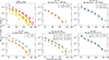 |
Fig. 13. Median radial profiles of the Lyα SB for bins of different quasar properties. The panels show the median Lyα SB corrected by cosmological dimming as a function of projected comoving distances within different bins, the error bars represent the mean 1σ uncertainty of the stacked data points. Top left: Median profiles within equally spaced bins of peak Lyα luminosity density of the quasars (see Section 4.1), color-coded by the median |

Additionally, we stacked the profiles in the same way but using equally spaced bolometric luminosity bins starting with ![Mathematical equation: $ \log(L_\mathrm{{bol}}/{[\rm{erg\,s}^{-1}]}) = 45 $](/articles/aa/full_html/2026/03/aa54054-25/aa54054-25-eq14.gif) to 48.7 and sizes of 0.6 dex, resulting in 5 bins with 8, 31, 21, 31 and 28 profiles each. We do not show these profiles, but we note that a similar trend is observed between the SB level and the bolometric luminosity as expected from the relationship between the bolometric luminosity and the peak Lyα luminosity density of the quasar (Figure 4).
to 48.7 and sizes of 0.6 dex, resulting in 5 bins with 8, 31, 21, 31 and 28 profiles each. We do not show these profiles, but we note that a similar trend is observed between the SB level and the bolometric luminosity as expected from the relationship between the bolometric luminosity and the peak Lyα luminosity density of the quasar (Figure 4).
It is clear from these observations that the Lyα SB level of the nebulae is correlated with the quasar luminosities. We test whether other AGN properties could also be responsible for the changes in SB level. For this, we constructed additional bins at different black hole masses and Eddington ratios that span the range of properties of the targeted quasars. These bins are overlaid and labeled in the left panel of Figure 12. Bins A1 and A2 are constructed to cover the low end of bolometric luminosities (Lbol ∼ 1046 erg s−1) and black hole masses between MBH ∼ 108.1 − 8.6 and ∼ 108.6−9.5 M⊙, respectively. Bins A3, A4 and A5 are constructed to cover the higher end of bolometric luminosities (Lbol ∼ 1047.5 erg s−1) and black hole masses of MBH ∼ 109.0 − 9.4, ∼109.4 − 9.7 and ∼ 109.7−10.2 M⊙, respectively. Bins B1, B2, B3 and B4 are constructed to cover the lower end of Eddington rations (λEdd ∼ 0.2) and black hole mass bins of log(MBH/M⊙) = 8.3 to 10.3 and sizes of 0.5 dex. Finally, bins B5 and B6 are constructed to cover the higher end of Eddington ratios (λEdd ∼ 1.0) and black hole mass bins of log(MBH/M⊙) = 8.9 − 9.4 to 9.4 − 9.9. We stress once again that the uncertainties in the estimation of the black hole masses and bolometric luminosities are about 0.5 and 0.3 dex, respectively (Section 2.2). This is why we conservatively adopt these large bin sizes.
We stacked the Lyα SB profiles inside these bins using the same aforementioned method and plot the resulting profiles in Figure 13, where each panel corresponds to a set of bins indicated in their legend. The top middle panel of this figure shows that the increasing black hole mass at low bolometric luminosity (bins A1 and A2) does not have an impact in the median SB profile, indicating that the Lyα radiation around faint quasars is independent of the black hole mass. Similarly, at high bolometric luminosity but different black hole mass (bins A3, A4, A5) there is no apparent evolution of the profiles. The bottom left panel of Figure 13 shows, however, that at fixed black hole mass (MBH ∼ 109 M⊙), the lower end of bolometric luminosities (bin A2) has around 7 times dimmer nebulae than the higher end of bolometric luminosities (bin A3), confirming the trend observed between individual radial profiles and bolometric luminosity of Figure 10. On the other hand, if we compare the bins with low Eddington ratios and different black hole masses (bins B1, B2, B3 and B4) we see a slight increase in the SB level of the stacked profiles, more likely originating from the increase in bolometric luminosity than the increase in black hole mass, as we do not see changes in profiles due to black hole mass in other plots. Finally the two bins at high Eddington ratio (B5 and B6) show very similar profiles despite the different black hole mass and slightly different bolometric luminosity.
Additionally, we used the same bins to compute median Lyα velocity dispersion radial profiles which are shown in Figure 14 using the same colors as in Figure 13. The stack is carried out by computing the median value at each projected distance bin and masking out values that fall below the spectral resolution limit (σ = 72 km s−1 at the median redshift for Lyα). These plots show that all profiles seem to approach the resolution limit at projected comoving distances between 100 and 200 kpc. Additionally, we see that the velocity dispersion profiles follow similar trends as the SB radial profiles as a function of bolometric luminosity. The velocity dispersions become higher toward the center with increasing peak Lyα luminosity density of the quasar and bolometric luminosity. This effect is clearly seen in the bottom left panel where the velocity dispersion increases from 300 km/s to 500 km/s in the center for bins A2 and A3, respectively. This trend can be understood as an effect of AGN activity on the CGM kinematics. Similarly to Figure 13, the profiles do not seem to be strongly affected by the change in black hole mass.
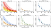 |
Fig. 14. Median radial profiles of the Lyα velocity dispersion for bins of different quasar properties. The panels show the median velocity dispersion of the Lyα nebular line as a function of projected comoving distances within the same bins, layout and colors as Figure 13. The error bars represent the uncertainty obtained from the 16 to 84 percentile of the stacked data points. In each panel, the shaded gray regions mark the values below the spectral resolution limit of the observations. Additionally, we show in the leftmost column the resulting power law fits in comoving distance units of the form σ = σ50(r/50 kpc)−β to the median profiles with a solid curve and shaded regions indicating their 1σ uncertainties (see text for details). |
Finally, given the large intrinsic uncertainties in the quasar parameters, we test how the stacked profiles change by varying the positions of each system in the log(MBH/M⊙)–log(Lbol/L⊙) plane (Figure 12). Specifically, we verify this for the bins where we see most of the variation: bins A2 and A3. We generated A2 and A3 samples by randomly drawing the individual values from Gaussian distributions defined by the intrinsic uncertainties in the estimators and centered on the data points in Figure 12. For each random realization of the plot in Figure 12 we stacked the profiles of sources within the A2 and A3 ranges. This process is repeated 2000 times. We find that the median profiles and uncertainties obtained from this exercise are consistent with the ones presented in Figures 13 and 14.
4.1.2. Exponential and power-law fits to median profiles
With these tests we confirm that the increase in SB level and velocity dispersion of the nebulae is correlated to the bolometric luminosity, therefore we focus in quantifying these differences by fitting with a power or exponential law the median profiles inside the quasar luminosity bins described above. We performed the fits using a Markov Chain Monte Carlo (MCMC) approach, which is implemented in the emcee6 module for Python (Foreman-Mackey et al. 2013). First, we fitted the data using the curve_fit function of scipy (Virtanen et al. 2020) and use these to initialize the positions of the MCMC walkers. We generated 50 samples of each parameter and run the MCMC process on 20 000 steps. For reference, we show in the top left panels of Figures 13 and 14 the resulting exponential and power law fits, respectively, with a solid line and shaded regions representing their 1σ uncertainty and using the same colors as the data points of each corresponding median profile. Additionally, we fitted the median profiles of the nondetections, bin A2 and bin A3 with the same method. For the Lyα SB corrected by cosmological dimming, we fitted the profiles (in comoving units) using both a power law of the form SBLyα(1 + z)4 = SB0 × rβ and exponential function of the form SBLyα(r) = SB0 × e−(r/Rh). On the other hand, for the median velocity dispersion profiles within the same comoving bins, we fitted only a power law of the form σ = σ50(r/50 ckpc)β.
We summarize in Table 1 the resulting fitted parameters to the radial profiles stacked in the different bins described in this section. Additionally, Figure 15 shows the results of the MCMC fit to these bins. In that figure, each panel shows the fits inside  and Lbol bins with a dot-dashed red line and solid blue line, respectively. The top row shows the power law fit parameters to the stacked SB profiles, where we see that the normalization factor SB0 of the median profiles tends to increase up to an order of magnitude with increasing quasar luminosity and the power β ranges between −2.25 to −1.75. Similarly, the middle row shows the fitted parameters for the exponential function, which shows a similar behavior in the normalization factor. The characteristic radius Rh of the exponential fit appears to be constant at ∼12.5 kpc (∼50 ckpc). The fitted parameters of the stacked nondetections are shown with a white diamond, while the fits of bins A2 and A3 are shown with light blue and dark blue squares. The fitted values for these three bins follow similar tendencies as the luminosity bins. The profile obtained by stacking the nondetections has a lower normalization factor than the lowest luminosity bin (which has comparable median luminosity), suggesting that these systems could be at the faint end of the nebula distribution. It is also possible, however, that at low luminosities, some mechanisms can suppress the observed extended Lyα emission, such as host galaxy orientation (e.g., Costa et al. 2022), small opening angles (Obreja et al. 2024) and/or molecular and dust content of the host galaxy (Muñoz-Elgueta et al. 2022; González Lobos et al. 2023), which we further discuss in Section 4.3.
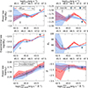 |
Fig. 15. Fit parameters from a power and exponential law to the stacked SB and velocity dispersion profiles as functions of their median quasar luminosities. The first row shows the fitted log(SB0) (left) and β (right) parameters of a power law versus the median peak Lyα luminosity density (top axis, dot-dashed red line) and bolometric luminosity (bottom axis, blue line) of the quasar, with their respective uncertainties as shaded areas. The second row shows the log(SB0) and Rh parameters of an exponential law fit as a function of their median quasar luminosities. The bottom row shows the fitted log(σ50) and β of a power law fit to the median velocity dispersion profiles as a function of their quasar luminosity. We also show in the left panel a power law fit to the normalization factor as a function of bolometric luminosity of the form |
![Mathematical equation: $ \sigma_{50}=\sigma_\mathrm{{bol}}(L_\mathrm{{bol}}/{[10^{46}\,\rm{erg\, s}^{-1}]})^\alpha $](/articles/aa/full_html/2026/03/aa54054-25/aa54054-25-eq16.gif)
Best parameters of the MCMC fits to the median radial profiles of Lyα SB and the velocity dispersion for different quasar luminosity bins.
Additionally, we assess the goodness of the power law versus exponential fits to each stacked profile by calculating the root-mean-square-deviation (RMSD) between the profiles and their fitted functions and weighted by the data uncertainty σ as
 (6)
(6)
The results of the RMSD calculation to each fit are presented in Table 1. We find that the exponential function is a better fit to the profile of stacked nondetections than a power law (RMSD of 2.9 and 4.2, respectively). Similarly, bin A2 is also better described with an exponential than power law (RMSD of 1.6 and 3.3, respectively). Opposite to this, bin A3 is better described with a power law rather than an exponential law (RMSD of 3.6 and 13.04, respectively). This is a consequence of the increased SB toward the center in comparison to the points at larger distance (see Figure 13), which biases the fit toward larger normalization factors. If this first point is not considered in the fit, an exponential law can be a good description of the profile in bin A3. Finally, the bottom row of Figure 15 shows the fitted parameters to the median velocity dispersion profiles for a power law of the form σ = σ50(r/50 ckpc)β. From the bottom right panel, we see that the power remains basically constant at β ∼ −1.0. On the other hand, the normalization factor σ50 is related to the bolometric luminosity through a power law. Therefore, we further fit a power law of the form ![Mathematical equation: $ \sigma_{50}=\sigma_\mathrm{{bol}}(L_\mathrm{{bol}}/[\mathrm{{erg\,s}^{-1}}])^\alpha $](/articles/aa/full_html/2026/03/aa54054-25/aa54054-25-eq20.gif) and show the result in that panel with a dashed black line, together with a list of the parameters values in the legend (α = 0.2928 ± 0.0003, σbol = 225.0 ± 0.2 km s−1). This indicates that all of the observed inner velocity dispersions have a clear scaling with the quasar bolometric luminosities, suggesting that the Lyα emission could be tracing the impact from AGN radiation and/or winds/outflows at these scales. This finding could be used in future works to test AGN feedback models and their energy coupling with the gas.
and show the result in that panel with a dashed black line, together with a list of the parameters values in the legend (α = 0.2928 ± 0.0003, σbol = 225.0 ± 0.2 km s−1). This indicates that all of the observed inner velocity dispersions have a clear scaling with the quasar bolometric luminosities, suggesting that the Lyα emission could be tracing the impact from AGN radiation and/or winds/outflows at these scales. This finding could be used in future works to test AGN feedback models and their energy coupling with the gas.
To understand whether the inner velocity dispersions are a possible sign of outflowing gas, we compare them to the average one-dimensional root mean square (rms) velocity of a massive MDM ∼ 1012.5 M⊙ halo expected to host these quasars. A velocity dispersion comparable or smaller than this value should indicate gravitational motions, while larger values candidate outflowing gas. Given that the maximum of the average 1D rms velocity σrms − 1D is related to the maximum circular velocity within a dark matter halo by  (Tormen et al. 1997), assuming such a massive halo at z ∼ 3 characterized by an NFW profile (Navarro et al. 1997) with a concentration parameter of c = 3.7 (Dutton & Macciò 2014), the maximum circular velocity is
  km s−1, giving
  (similar calculation in Arrigoni Battaia et al. 2019a). This value corresponds to log Lbol/L⊙ = 46.15 in the obtained power-law relationship. This bolometric luminosity is similar to the median bolometric luminosity of the QSO MUSEUM faint sample (
 ), for which we observe lower inner velocity dispersions (σ ∼ 300 km s−1), suggesting that these systems could be less affected by AGN feedback. Conversely, the more luminous quasars in the sample may have imprinted the signature of AGN feedback in their associated extended emission, which is distinguished by elevated inner velocity dispersions (σ ∼ 600 km s−1; Figs. 12 right and 14). This finding has to be tested with nonresonant lines as the velocity dispersion is likely increased by resonant scattering effects (e.g., Figure B1 in Costa et al. 2022). Robustly, the Lyα emitting gas at projected distances larger than 30 kpc seems to be dominated by gravitational motions (σ < 250 km s−1).
4.2. Evidence of instantaneous AGN feedback on circumgalactic scales
AGN feedback is a key ingredient of galaxy formation models, especially for reproducing the massive end of the galaxy population (e.g., Di Matteo et al. 2005). Nevertheless, there is still considerable debate regarding the impact of AGNs on their host galaxies and the surrounding medium (e.g., Harrison & Ramos Almeida 2024). One key issue is the lack of conclusive observations of the instantaneous, rather than cumulative, effects of AGNs on large scales. Such observations are essential to determine how the energy couples with the gas, and ultimately how AGN feedback works. In this section, we discuss the evidence for likely instantaneous AGN feedback and its impact on CGM scales as traced by the Lyα emission, considering that all of our targets are quasars expected to be in the radiatively-efficient regime (e.g., Harrison & Ramos Almeida 2024).
We discussed that the observed Lyα and bolometric luminosity of the quasars have the strongest relation with the SB and velocity dispersion of the extended Lyα emission (Section 4.1). In other words, brighter (more accreting) quasars, expected to generate stronger feedback, are associated with brighter and more turbulent extended Lyα emission. These results were not obvious a priori. The fact that these relations are in place implies that the mechanisms responsible for the Lyα emission act on timescales similar to the known variability of quasar activity as otherwise any relation with the observed current quasar activity would be washed out. Given the rather short quasar variability estimates (see Section 1), the observed relations between quasar luminosity and CGM emission seems an indication of instantaneous AGN feedback.
For example, if we assume that the nebulae are predominantly powered by photoionization followed by recombination, then a drop in luminosity due to the shutdown at the end of their current quasar activity could cause small Lyα nebulae, or parts of them, to fade. We do not see this effect, however,. For this to occur, the recombination time needs to be much shorter than the period of shut-down, which has been inferred to be about 104 − 5 years by some observations (e.g., Lintott et al. 2009; Davies et al. 2015). The timescale for case B recombination is trec = 1/αB(T)nH where nH is the gas number density and  is the recombination coefficient (Dijkstra 2019). Then, for this phenomenon to occur in 2 × 10⁴ K gas, the Lyα would be tracing volume densities of nH ≫ 2 cm−3. The fact that we do not find nondetections or donut-like shaped Lyα nebulae (i.e., the inner portion of the CGM would be the first to decrease in SB after the turn off of a quasar) among most quasars seem to confirm that the quasar shut-down phases, if any, are very short and much shorter than the recombination time in the Lyα emitting gas. This means that the densities of the Lyα emitting gas are not as high.
Figure 16 summarizes the AGN electromagnetic impact on the Lyα SB and velocity dispersion median radial profiles by focusing on the bins A2 and A3, which were constructed at roughly fixed black hole mass (MBH ∼ 109 M⊙) and increasing bolometric luminosity, hence Eddington ratio λ = 0.2 and λ = 0.9, respectively. The left panel shows the median Lyα SB corrected by cosmological dimming as a function of projected distance, with the shaded areas representing the 25 and 75 percentiles of the stacked profiles. Additionally, we show the median Lyα SB profile of the stacked nondetections with gray dots and shaded region indicating its 1σ uncertainty. For comparison, we show in the same panel the simulated profile obtained in Obreja et al. (2024) by assuming that the cool CGM of a high-resolution zoom-in 1012.45 M⊙ halo is only illuminated by the ultraviolet background (UVB) (dashed red curve). The simulation has been run only with stellar feedback down to z ∼ 3, but it is in agreement with the halo mass – stellar mass relation (Moster et al. 2018). This profile has a similar scaling to the stacked profile of nondetections, but decays more steeply with increasing radius. Suggesting that even faint quasars can affect the surrounding cool CGM emission.
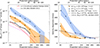 |
Fig. 16. Median Lyα SB and velocity dispersion of the stacked radial profiles. Left: Lyα SB corrected by cosmological dimming as a function of projected comoving distance for the stacked nondetections in gray dots and bins A2 and A3 with orange and blue triangles, respectively. The simulated Lyα profile obtained from the illumination of a 1012.45 M⊙ halo by only the UVB (Obreja et al. 2024) is shown with a dashed red line. The profile around LBGs (Steidel et al. 2011) is shown with a magenta line. Right: Velocity dispersion as a function of projected comoving distances of bins A2 and A3 with orange and blue triangles, respectively, and their shaded region representing the 25th to 75th percentiles. Additionally, we show with a dashed black line and a dot-dashed red line the intrinsic Lyα velocity dispersion (σint) from de Beer et al. (2023) using cosmological simulations of halos at z = 3.017 with Mhalo = 1012 and 1012.6 M⊙, respectively, after rescaling to match the velocity dispersion at 17 kpc of bin A2 (see Section 4.3). The median bolometric luminosity and Eddington ratio for the sources in bins A2 and A3 are indicated in the legend. |
Last, as reference, the Lyα SB profile around Lyman break galaxies (LBGs; Steidel et al. 2011) is shown in the same panel with a solid magenta line. LBGs are expected to be hosted in less massive (MDM ∼ 1012 M⊙) and less active halos than those hosting quasars.
The right panel of Figure 16 shows the median velocity dispersion profiles within the same bins, with shaded areas representing their 25 and 75 percentiles. The velocity dispersion in bin A2 is on average a factor of 2× lower than the velocity dispersion of bin A3. Both profiles drop quickly from the inner regions and seem to plateau at larger radii, with the latter effect likely due to the instrument spectral resolution. Given that bins A2 and A3 span a similar range of black hole masses, the difference in the central velocity dispersion (< 40 kpc) could indicate that the inner CGM turbulence is modulated by the intensity of AGN feedback in these systems, and that the Lyα emission better traces the violent AGN impact on these inner CGM scales. The quasar lifetimes quoted in Section 1 (∼107 years) are compatible with the time that an outflow with 1000 − 5000 km s−1 requires to reach the observed CGM scales (10 − 50 kpc). Therefore, the found power law relating the velocity dispersion to the bolometric luminosity (section 4.1 and Figure 15) could be used in future works to test AGN feedback models and their energy coupling with the cool gas.
It is important to note that the velocity dispersion of extended Lyα emission around quasars has been frequently associated with gravitational motions within massive halos of Mhalo ∼ 1012.5 M⊙, both using averages over the full detected nebulae (Arrigoni Battaia et al. 2019a; Farina et al. 2019) and the ratio of the median velocity dispersion in two specifically selected radial annuli (de Beer et al. 2023). The latter work assumed that the intrinsic Lyα velocity dispersion profiles obtained from their cosmological hydrodynamic simulations under the assumption of only quasar photoionization followed by recombination can be simply scaled in normalization to match observations, and therefore estimate the halo mass. The right panel of Figure 16 shows the simulated intrinsic Lyα velocity dispersion (σint) from de Beer et al. (2023) using mock observations of cosmological simulations of halos of M = 1012 and 1012.6 M⊙ at z = 3.017 with a dashed black line and dot-dashed red line, respectively, after rescaling them to match the observed velocity dispersion at an average projected distance of 17 kpc (or ∼70 ckpc) of bin A2. This normalization considers that de Beer et al. (2023) used as first radial annuli for their ratio calculation the range of projected comoving distances of 40–100 kpc, corresponding to 9.76-24.4 kpc at the median redshift of our sample. Their simulated profile is much broader than the one observed here, indicating that their working assumptions cannot be entirely valid.
Additionally, it has been long ago proposed a correlation between the SMBH mass and the mass of the host dark matter halo (Ferrarese 2002), and this relation should be tighter at earlier cosmic times (Volonteri et al. 2011). As proposed by Farina et al. (2022) one could obtain a first estimate of the halo circular velocity under the assumption that the extended Lyα emission traces on average gas in gravitational motion within the dark matter halo. We attempted such a calculation for our sample and found no strong correlation and a similarly large scatter as in Farina et al. (2022) (see their Figure 13). This fact could be due to the large uncertainties in SMBH mass values and on the use of an average velocity dispersion which could be dominated by more violent kinematics around highly accreting sources. Observations targeting lower SMBH masses are needed to test the presence of this relation and its evolution (if any) at z ∼ 3.
Given the lack of agreement with gravitational effects, we propose that other mechanisms, like the AGN activity earlier discussed, could be contributing to the observed inner shape of the velocity dispersion profile. Particularly, the regions more sensitive to AGN impact (R < 40 kpc) seem to be where the nebulae appear more circular, while larger scales are tracing more quiescent material. In the following section, we discuss the different possible roles of this AGN feedback in powering extended Lyα emission.
4.3. Insight into the mechanisms that power the extended Lyα emission
As mentioned in Section 1, there are several physical mechanisms that can collectively power the observed extended Lyα emission, such as photoionization due to the quasar (and nearby sources) radiation followed by recombination, resonant scattering of Lyα photons originating from the BLR of the quasar, shocks due to galactic/AGN winds and outflows, and gravitational cooling. In Section 4.1, we proposed that the observed Lyα SB and velocity dispersion are modulated by the central AGN due to their dependence with the bolometric luminosities of the quasars at fixed black hole masses. Given this dependence, we exclude a gravitational cooling scenario, which would instead depend mainly on the halo mass of the system studied (e.g., Dijkstra & Loeb 2008; Faucher-Giguère et al. 2010). Next, we discuss the interplay that can happen between AGN luminosities and the remaining powering mechanisms, and ultimately their possible contribution to the observed extended emission.
4.3.1. Photoionization due to AGN radiation followed by recombination
In this scenario, gas illuminated by any quasar considered in this work is expected to be almost fully ionized (Mackenzie et al. 2021), and optically thin to ionizing radiation. This results in a Lyα SB level that depends on the gas properties such as hydrogen volume and column densities (SBLyα ∝ nHNH; Equation 10 in Hennawi & Prochaska 2013), translating to a dependence in nH and mass reservoir in the cool phase MH. First, we can assume a fixed MH represented by the median value of column density obtained in absorption studies of quasar CGM, NH = 1020.5 cm−2 (Lau et al. 2016). This value is obtained from optically thick absorbers located along transverse directions to the quasars, and hence likely not illuminated (Hennawi & Prochaska 2007). However we assume that the total hydrogen column is the same for illuminated and not illuminated regions. Using this value of NH, we find that the median Lyα SB profiles of the faint and bright quasar nebulae imply gas densities of nH ∼ 0.5 and 2 cm−3, respectively, assuming a fixed projected distance of R ∼ 20 kpc, the median redshift of our sample, and a covering fraction of fC = 1 (Arrigoni Battaia et al. 2015a). As expected, these values are consistent with the densities estimated in previous works (e.g., Hennawi et al. 2015; Arrigoni Battaia et al. 2019b). Thus, if the recombination scenario in optically thin gas were the dominant mechanism powering the nebulae, then the observed Lyα SB may imply that the bright quasars reside in denser gas reservoirs. Similarly, if we repeated the same calculation, but fixed nH, the change in SB could be due to a more (4×) massive reservoir of cool gas around bright quasars. The faint and bright quasars at z ∼ 3 seem to reside in similarly massive halos, however, as estimated by clustering measurements (White et al. 2012; Timlin et al. 2018). At low redshift, the black hole mass also scales with the halo X-ray temperature, hence halo mass (e.g., Gaspari et al. 2019). If this relation holds also out to z ∼ 3, we should see a trend of increasing velocity dispersion as a function of black hole mass if the velocity dispersion of Lyα nebulae is a proxy of quasar halo mass (Arrigoni Battaia et al. 2019a; Farina et al. 2019; de Beer et al. 2023). Here, we do not see strong evidence for such a trend (see Figure 14). Hence, we do not expect drastic changes in nH and MH in the targeted quasars, unless the effect of quasar feedback is considered. Brighter quasars might increase densities in the inner halo because of entrained material in stronger winds/outflows (e.g., Costa et al. 2014), but can simultaneously reduce the reservoir of cool gas due to stronger ionizing radiation (e.g., Obreja et al. 2024). Alternatively, other mechanisms, such as stripped satellite galaxies, could supply additional gas mass to power the observed nebulae. This effect would need to be more pronounced around brighter quasars, however, which requires further observational tests (e.g., Chen et al. 2021; Bischetti et al. 2021). Another way to vary the cool gas mass as a function of quasar luminosity is to assume a change in the fraction of gas illuminated by the AGN (Obreja et al. 2024), e.g., by requiring that the ionization cone angle increases with bolometric luminosity. We further discuss this in Section 4.3.4.
4.3.2. Resonant scattering of Lyα photons from the BLR of the quasar
In this scenario, Lyα photons originating from the BLR of the quasar scatter through the surrounding medium until they escape the CGM. Therefore, the observed flux distribution contains information on the Lyα source as well as the location and kinematics of the last scattering event (see e.g., Blaizot et al. 2023). In this case, we expect that the Lyα luminosity of the nebulae is correlated to the amount of Lyα photons originating from the quasar (and consequently Lbol, Figure 4).
To test this scenario, we compare with a high-resolution cosmological, radiation-hydrodynamic simulation of a quasar host halo at z > 6 post-processed with a Lyα radiative transfer code Costa et al. (2022). Their predictions were able to match the Lyα emission out to scales of ∼100 kpc in z ∼ 6 quasar host halos. These simulations indicated that BLR photons, even alone, can power Lyα nebulae. Additionally, they proposed that AGN outflows are essential for the formation of extended Lyα emission, by clearing out the gas within the galactic nucleus and allowing Lyα photons to scatter through the CGM. This could be consistent with our observations, which show that an increase in the luminosity of the quasar or its Eddington ratio (hence AGN feedback) corresponds to brighter nebulae with larger velocity dispersions at their center, which could arise in the case of AGN winds/outflows injecting turbulence into the ISM and CGM cool gas. The simulations from Costa et al. (2022) predicted that only quasar photons with |Δv|≲1000 km s−1 scatter and create Lyα nebulae, while photons in the broad wings usually freely stream through the CGM. We test this by comparing in the top panel of Figure 17 the ratio of the Lyα FWHM of the nebulae (computed from the average of the second moment maps) and the Lyα FWHM of the quasars (see Appendix B for an explanation of its calculation) as a function of Lbol, where the data points are colored by their black hole mass. In the same panel, the median values of bins A2 and A3 are shown using blue squares and error bars representing the full range of values within the bin. The plot shows that the Lyα extended emission always has a width narrower than that of the quasar line, ranging from about 50% to 2%, in agreement with the expectations from this scenario. Additionally, at fixed black hole mass (bins A2 and A3), a higher Eddington ratio corresponds to an increase of the ratio of the FWHMs. Once taking into account the drop in FWHM for these bins, there is still a residual increasing trend suggesting that the FWHMneb around more accreting systems encodes information on the impact from AGN feedback on the CGM kinematics as we have discussed earlier in Section 4.2. Alternatively, it could also be possible that larger FWHMneb appear around brighter quasars because of the increased amount of BLR Lyα photons available for scattering and/or higher amounts of gas (and optical depth) in the vicinity of these AGNs.
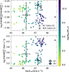 |
Fig. 17. Lyα FWHM vs. bolometric luminosity. In both panels each star represents a system with nebula detected and colors indicating the black hole mass. Additionally, we show in both panels the median values of bins A2 and A3, with their error bars representing the full range of values in the bin. Top: Ratio of the Lyα FWHM of the nebula, computed from the mean velocity dispersion of the second moment maps (Figures 8 and C.6), and the Lyα FWHM of the quasar as a function of bolometric luminosity. Data points obtained from the z ∼ 6 cosmological simulations in Costa et al. (2022) considering all powering mechanisms (white plus) and scattering from the BLR only (white cross). Bottom: FWHM of the Lyα line of the quasar (Tables B.1 and B.2) as a function of the bolometric luminosity of the quasar (see Appendix B). |
The bottom panel of Figure 17 shows that faint and bright quasars span the whole range of measured FWHM and there is no clear indication of a correlation with their bolometric luminosity. Quasars displaying a stronger Lyα FWHM tend to also have relatively higher black hole masses at fixed bolometric luminosity, however, as expected from BH virial mass estimators. For comparison, the data points from the z ∼ 6 cosmological simulation of Costa et al. (2022) (Table 2 in that work) considering all powering mechanisms (recombination, collisions, broad-line region scattering) and only broad-line-region scattering of Lyα photons are shown in the top panel with a white plus sign and white cross, respectively. These simulations assumed in input for the radiative transfer calculation that
  , MBH ∼ 109 M⊙ and Lbol = 3 × 1047 erg s−1, which are comparable to the values of the high accreting bin A3. The linewidth ratios from the simulation are comparable to the measured values, but from this observation it is not possible to disentangle the mechanisms. This is even more true considering the variations in the FWHM when observing the simulated system adopting different line of sights (the standard deviation of the FWHM values along the six line of sights studied in Costa et al. (2022) is of about 150 km/s).
Having demonstrated that the FWHM ratio is comparable with predictions for a broad-line region photon scattering scenario, we further test this case by using the same approach from González Lobos et al. (2023) and compute in first approximation the number of BLR Lyα photons available for scattering  . For this, we integrated the quasar spectra within ±FWHM of the nebular Lyα line and compare it with the integrated Lyα luminosity of the nebula within the same velocity range (Tables A.2 and C.1). The top panel of Figure 18 shows that these two quantities are positively correlated, consistent with González Lobos et al. (2023) and our results on the SB profiles. Moreover, the Spearman rank correlation coefficient between
  and
and  is 0.8, indicating a very strong positive correlation. The relationship is fitted with a power law of the form
 ![Mathematical equation: $ L_\mathrm{{Ly}\alpha}^\mathrm{{neb}}/[10^{44}\,\mathrm{{erg\,s}^{-1}}]=L_0(L_\mathrm{{bol}}/[10^{45}\,\mathrm{{erg\,s}^{-1}})^\alpha $](/articles/aa/full_html/2026/03/aa54054-25/aa54054-25-eq32.gif) , where L0 = 0.70 ± 0.05 and α = 0.51 ± 0.05, and shown with a dashed black line. Additionally, the values of bins A2 and A3 are shown with blue squares and error bars indicating the full range of values within each bin. The found relation could be a hint that broad-line region photons scattering is in place. Because quasars with stronger ionizing radiation can reduce the amount of neutral hydrogen (Obreja et al. 2024) available for scattering, however, the ratio of
, where L0 = 0.70 ± 0.05 and α = 0.51 ± 0.05, and shown with a dashed black line. Additionally, the values of bins A2 and A3 are shown with blue squares and error bars indicating the full range of values within each bin. The found relation could be a hint that broad-line region photons scattering is in place. Because quasars with stronger ionizing radiation can reduce the amount of neutral hydrogen (Obreja et al. 2024) available for scattering, however, the ratio of  and
and  should decrease with increasing ionizing radiation. The bottom panel of Figure 18 shows this behavior, where the Lyα luminosity ratio (fraction of scattered quasar photons) tends to decrease with increasing Lbol. For this case we also computed the Spearman rank correlation coefficient and find a value of −0.73, indicating a strong negative correlation. A power law fit of the form
 ![Mathematical equation: $ (L_\mathrm{{Ly}\alpha}^\mathrm{{neb}}/L_\mathrm{{Ly}\alpha}^\mathrm{{QSO}}) = A(L_\mathrm{{bol}}/[10^{47}\,\mathrm{{erg\,s}^{-1}}])^\beta $](/articles/aa/full_html/2026/03/aa54054-25/aa54054-25-eq35.gif) with values A = 0.07 ± 0.01 and β = −0.43 ± 0.05 is shown with a dashed black line. Together, these relations are suggestive of a contribution from resonant scattering of the quasar Lyα photons to the overall extended Lyα emission. We note that the ratio
with values A = 0.07 ± 0.01 and β = −0.43 ± 0.05 is shown with a dashed black line. Together, these relations are suggestive of a contribution from resonant scattering of the quasar Lyα photons to the overall extended Lyα emission. We note that the ratio  is a proxy for the scattered photon fraction, but not its actual value, due to the way it has been estimated, especially the lack of modeling of the intrinsic Lyα emission of the quasar. In a pure resonant scattering scenario, the fraction of scattered photons should depend on the Lyα optical depth of the residual neutral fraction, which would be inversely proportional to the ionizing luminosity. The shallower slope of β = −0.43 that we observe is likely influenced by uncertainties in the estimation of both the ratio (i.e., the quoted
  does not represent the total intrinsic quasar luminosity) and Lbol. With a more reliable estimate of the ratio, a shallow slope would suggest that other mechanisms besides resonant scattering are also at play.
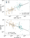 |
Fig. 18. Comparison of nebular luminosities as a function of quasar luminosities. Top: Lyα luminosity of the detected nebulae versus Lyα luminosity of the quasar, integrated within the ±FWHM range of the nebular Lyα line (see Section 3.3 and Tables A.2 and C.1) and error bars representing the 1σ uncertainty of the measurements. The median luminosities of bins A2 and A3 are shown with blue squares and their error bars represent the full range of values within each bin. Additionally, we plot with a dashed black line a power law fit of the form |
![Mathematical equation: $ L_\mathrm{{Ly}\alpha}^\mathrm{{neb}}/[10^{44}\,\mathrm{{erg\,s}^{-1}}]=L_0(L_\mathrm{{bol}}/[10^{45}\,\mathrm{{erg\,s}^{-1}}])^\alpha $](/articles/aa/full_html/2026/03/aa54054-25/aa54054-25-eq38.gif)
![Mathematical equation: $ (L_\mathrm{{Ly}\alpha}^\mathrm{{neb}}/L_\mathrm{{Ly}\alpha}^\mathrm{{QSO}}) = A(L_\mathrm{{bol}}/[10^{47}\,\mathrm{{erg\,s}^{-1}}])^\beta $](/articles/aa/full_html/2026/03/aa54054-25/aa54054-25-eq39.gif)
Finally, as a last test, we hypothesize that resonant scattering of Lyα should result in an increase in nebular FWHM compared to a recombination-only scenario (see, for example, Costa et al. 2022), and that this increase should be more pronounced when more Lyα photons are available. The top panel of Figure 19 shows the FWHM of the Lyα line for each nebula as a function of the bolometric quasar luminosity, color-coded according to the percentage of the quasar Lyα luminosity (integrated within the  , see Section 3.3) relative to the bolometric quasar luminosity (see Section 2.2). The median values of bins A2 and A3 are shown as blue squares, with error bars representing the uncertainty in Lbol. At fixed Lbol, the ratio of the two luminosities increases in average. This indicates that quasars with more Lyα photons available for scattering have broader nebulae. To quantify this further, we fitted a power-law relationship between the nebular FWHM and Lbol (dashed gray line) and computed the distance if FWHM to it. The result is shown in the bottom panel of Figure 19, where darker points (larger luminosity ratio) have, on average, positive differences with respect to the dashed line. There is significant scatter, however.
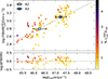 |
Fig. 19. Lyα FWHM as a function of quasar luminosities. In both panels each star represents a system with nebula detected and colors correspond to the percentage of the quasar Lyα luminosity (integrated within the ±FWHM of the nebula) with respect to the bolometric luminosity. Top: Lyα FWHM at the center of the nebula, computed from the first point in the velocity dispersion radial profiles (Figure 11) as a function of bolometric luminosity of the quasar. The median values of bins A2 and A3 are indicated with blue squares and error-bars indicating the range of Lbol within each bin. The dashed gray line represents a power law fit to the data points. Bottom: Distance from the data points to the power law fit shown in the top panel. |
4.3.3. Shocks due to galactic/AGN outflows
Fast shocks are expected to provide additional ionizing photons and boost collisions. In such a case, the Lyα flux is expected to scale as FLyα ∝ nHvshock3, where vshock is the shock speed (Allen et al. 2008). Given the presence of increased Lyα SB around more accreting and hence active quasars, we cannot exclude shocks and collisions in powering the observed Lyα nebulae. If only shock speed would be responsible for the difference in Lyα SB in the A2 and A3 bins, bright quasars would push 2× faster outflows at fixed nH. This is not far from the debated scaling invoked by Fiore et al. (2017) between Lbol and the outflow velocity vout, with  . While this relation, if valid, is computed on smaller scales, it could be that shock velocities may follow similar relations and therefore contribute to the powering of the Lyα nebulae. The exquisite spatial resolution of JWST (Gardner et al. 2006) may help us in uncovering morphological and velocity signatures of shocks in the Lyα nebulae surrounding quasars as traced by rest-frame optical emission lines (e.g., [OIII], Peng et al. 2025).
Further, winds/outflows from an AGN can cause the peak of the observed Lyα flux distribution to appear redshifted with respect to the intrinsic emission due to Lyα resonant scattering (see e.g., Chang et al. 2023; Chang & Gronke 2024). In Figure 20, we show the distribution of velocity shifts (Δvm1) of the nebulae computed from the first moment of their Lyα flux distribution with respect to the peak Lyα wavelength of the quasar listed in Tables A.2 and C.1 of the faint and bright quasars with green and orange bins, respectively. Additionally, the number of nebulae in bins A2 and A3 as a function of their median Δvm1 with error bars representing the velocity range covered by each bin are shown with blue squares. Most of the nebulae have redshifts similar to the quasar Lyα, but the bright quasar sample shows more systems with velocity shifts > 200 km s−1. This would be consistent with the proposed scenario in which the most luminous quasars are producing stronger feedback, resulting in a more redshifted Lyα emission with respect to fainter quasars. Additionally, we also studied the distribution of velocity shifts derived from the Gaussian fits (Δvgauss in Tables A.2 and C.1) and found consistent results. More precise information on the systemic redshifts of the quasars is needed to draw further conclusions.
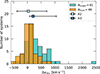 |
Fig. 20. Distribution of the Lyα nebula velocity shift with respect to the quasar Lyα emission peak. The plot shows histograms of the velocity shifts (vm1) computed from the first moment of the flux distribution (Tables A.2 and C.1) for the extended Lyα emission around the bright (green) and faint (orange) QSO MUSEUM samples. The size of each histogram bin corresponds to 163 km s−1. We also show the median vm1 for bins A2 and A3 (Figure 12) at the respective number of systems. Their error bars indicate the full range of velocity shifts within A2 and A3. |
4.3.4. A plausible simple scenario of an increasing quasar opening angle with bolometric luminosity
The previous subsections discussed evidence in favor of all the Lyα powering mechanisms related to AGN feedback, whether it pertains to electromagnetic (photoionization, BLR Lyα photon scattering) or mechanical (shocks) processes. In this subsection we assume that all these processes could act together and present a simple calculation to explain the uncovered observational trends.
The calculation is based on the idea proposed by Costa et al. (2022), which indicates that the observation of a Lyα nebula in the vicinity of a quasar requires the presence of an AGN outflow. Therefore, we compute whether the targeted quasars are capable of clearing out part of their host galaxy ISM. Specifically, Costa et al. (2018) estimated a bolometric luminosity threshold over which an AGN is able to power momentum-driven mechanical outflows, which can be computed as the luminosity at which the outbound radiation pressure acceleration balances the inward gravitational acceleration on the entirety of the ISM gas,
 (7)
(7)
where G is the gravitational constant, c the speed of light, RISM ≈ 0.1R200 is the outer boundary of the ISM, and MISM, M★ and MDM(< RISM) are the gas, star and dark matter masses within the ISM region. A typical z ∼ 3 quasar host dark matter halo has M200 = 1012.5 M⊙ and R200 ≈ 100 kpc. If we assume a Navarro-Frenk-White dark matter profile (Navarro et al. 1997) and use the concentration–halo mass relation for z = 3 of Dutton & Macciò (2014)MDM(< RISM)/M200 ≈ 0.056, we can estimate the ISM mass fraction MISM/M200 using the EAGLE simulation (the dashed green curve in figure 2 of Mitchell & Schaye 2022, for z = 2) to be 8% for our target halo mass, where we assumed the cosmic baryon fraction value of the Planck cosmology fb = Ωb/ΩM = 0.157. For the stellar mass fraction, we can use the z-appropriate relation of Moster et al. (2018) to get M★/M200 ≈ 0.027. Plugging all these numbers in the equation above, an AGN at z = 3 has to have a bolometric luminosity of at least Lths = 1.08 × 1048 erg/s for radiation pressure to push away all of the ISM. This limit luminosity is computed assuming a spherical symmetric ISM distribution. Quasars are typically associated with star-forming galaxies, however, which have their ISM organized in a disk. Therefore, the amount of ISM within the ionization bi-cone that needs to be removed for the AGN radiation to escape in free channels is lower. For example, if we assume the AGN needs to remove only the ISM within a typical ionization bi-cone of angle α = 60° (e.g. Obreja et al. 2024), the luminosity limit becomes [1-cos(α/2)] × 1.08 × 1048 erg/s = 1.4 × 1047 erg/s. Interestingly, this new luminosity threshold has the same order of magnitude of the minimum luminosity of the QSO MUSEUM I (bright quasar) sample7, which has larger average Lyα SB than the QSO MUSEUM faint sample as given, e.g., by the points’ sizes in Figure 12. The observed Lyα SB of the bright nebulae could then be produced because the AGN has been able to push enough ISM material. In turn this would make more efficient all the powering mechanisms related to AGN feedback: there will be (i) more ionizing photons escaping the galaxy and ionizing a higher mass of CGM gas (subsection 4.3.1), (ii) larger channels of least resistance for the propagation of Lyα photons (subsection 4.3.2), and (iii) faster shocks (subsection 4.3.3).
We stress that the CGM observations are sensitive to the illuminated volume or opening angle on halo scales after the AGN radiation escapes the host galaxy. While the unified model of AGN states that the opening angle is set by the small-scale torus (e.g., Netzer 2015), there is a growing body of literature showing that at higher redshift the host galaxies can contribute to the AGN obscuration, resulting in smaller opening angles or smaller fractions of illuminated volume (e.g., Circosta et al. 2019; Gilli et al. 2022). Therefore, AGN outflows are needed to clear the host ISM, and this will happen preferentially along directions where the resistance is lower even when assuming small scale isotropic AGN feedback (i.e., the minor axis in disk galaxies; Costa et al. 2014; Nelson et al. 2019).
Following this framework, we can roughly estimate the opening angle on CGM scales of the different samples by assuming that all the difference in the observed SB profiles is due to this effect. Specifically, if we assume that the observed ratio of SB profiles (7) between the low and high accreting quasars (bins A2 and A3, respectively) is due to the amount of AGN radiation able to escape, then the volume of illuminated ISM should scale accordingly. Approximating the ISM disk to a constant density and with an effective height of 2 kpc and considering an ionization bi-cone opening angle of 60° (Obreja et al. 2024) for the A3 quasars, we find that a factor of 7 times smaller volume illuminated would correspond to an opening angle of ∼25° for the A2 quasars. We note that equation 7 is only valid if the AGN outflow is produced due to radiation pressure, where the outward force is produced if every photon scatters only once. However, in very compact and dusty galaxies it is possible that reprocessed infrared photons are scattered multiple times by dust grains (Costa et al. 2018), which lowers the luminosity threshold needed to push out the galaxy ISM. Additionally, in the presence of energy-driven outflows (King 2003; Ward et al. 2024) it is possible to have an extra contribution to the outward force due to the shocked gas, which can lower the luminosity threshold by a factor of ∼10, as shown in simulations of z > 6 quasars (Costa et al. 2014, 2020). Taking into account these effects that would lower the luminosity threshold by at least a factor of ten, the A2 quasars would then have instead a bi-cone opening angle of at least 60°, and the increase of 7 times the illuminated volume would require opening angles of ∼113° for the A3 quasars.
Such large opening angles for brighter quasars are somewhat in tension with several previous studies (e.g., Hennawi & Prochaska 2013; Borisova et al. 2016; Obreja et al. 2024). However, it is acknowledged that the actual scenario may exhibit intermediate characteristics between these two regimes. Importantly, the scenario with smaller opening angles is consistent with the stacked SB profile of the quasars associated to nondetected nebulae (left panel of Figure 16) being slightly above the predictions presented in Obreja et al. (2024) for a AGN host halo illuminated by the UVB only8, which suggests that the fainter quasars could be at the lower end of the distribution of opening angles. In the current scenario, this implies that the faintest quasars have not been able to clear their surrounding ISM and produce channels for the ionizing radiation and Lyα photons to freely escape.
It has been argued that so different quasar opening angles might result in observable difference in the asymmetries of the nebulae (Mackenzie et al. 2021). However, our observations do not support the presence of such variations, which is consistent with earlier research. We hypothesize that the absence of observable differences can be attributed to the fact that at small opening angles, the level of emission is comparable to the level of Lyα emission resulting from other mechanisms, such as host galaxy star formation, cooling radiation, and UVB contribution, hence washing out any geometrical difference due to quasar illumination alone. The small opening angles for faint quasars can also explain the more frequent presence of narrow Lyα nebulae with very similar spectrum to some portions of the Lyα emission of the quasar itself (see Figures 6, A.1 and A.2). Such emission is likely due to ISM and inner CGM and potentially not illuminated by the quasar (see also Mackenzie et al. 2021). We stress that a luminosity dependent opening angle means that the fraction of obscured or type-II AGN fN would vary as a function of Lbol. Specifically, following geometrical arguments fN = cos(α/2) results in fNfaint = 0.98 and fNbright = 0.87 for the smaller opening angle scenario. These values are larger than those obtained using infrared luminosities and X-ray surveys (see, e.g., Figure 4 in Treister et al. 2008; Marconi et al. 2004; Merloni et al. 2014; Hickox & Alexander 2018), which would be more in agreement with the larger opening angle scenario. The rest frame UV might be more affected by obscuration than the wavelengths used in these studies, however. This can be tested with transitions in addition to Lyα.
Finally, if a change in opening angle is able to explain the difference of the SB profiles, it would imply that the radiation from the AGN is the main driver of the extended emission. The detailed contribution of recombination, shocks, and scattering of BLR Lyα photons is still unclear, however. Additional lines besides Lyα (e.g., HeII, Hα, [OIII]; e.g., Peng et al. 2025) or polarization measurements (e.g., Kim et al. 2025) can further help disentangle the different mechanisms. Even though there are still several uncertainties at play, we argue that statistical studies of quasar CGM could help in constraining the fraction of obscured AGN further.
5. Summary
We have presented the largest effort to date of mapping the CGM around quasars in Lyα emission, namely 120 z ∼ 3 quasars (QSO MUSEUM III). This effort builds upon our first sample around bright quasars (QSO MUSEUM I; Arrigoni Battaia et al. 2019a) and adds 59 new faint quasar fields. This results in a global sample with a median redshift of z = 3.13 and in bolometric luminosities, black hole masses, and Eddington ratios in the ranges ![Mathematical equation: $ 45.1 < \mathrm{{log}}(L_\mathrm{{bol}}/[\mathrm{{erg\, s}^{-1}]}) < 48.7 $](/articles/aa/full_html/2026/03/aa54054-25/aa54054-25-eq43.gif) , 7.9 < log(MBH/[M⊙]) < 10.3 and 0.01 < λEdd < 1.8. We were able to detect 110 Lyα nebulae around the 120 targets with a homogeneous strategy consisting of snapshot VLT/MUSE observations (45 minutes/source), totalling 120 hours of MUSE time when observation overheads are considered. All the nondetections are associated with the new faint sample. We characterized the Lyα SB level, kinematics, and morphology (area and asymmetry) of the extended emission, and searched for trends with quasar properties (luminosities, black hole mass, and Eddington ratio). Our observational results are summarized below.
, 7.9 < log(MBH/[M⊙]) < 10.3 and 0.01 < λEdd < 1.8. We were able to detect 110 Lyα nebulae around the 120 targets with a homogeneous strategy consisting of snapshot VLT/MUSE observations (45 minutes/source), totalling 120 hours of MUSE time when observation overheads are considered. All the nondetections are associated with the new faint sample. We characterized the Lyα SB level, kinematics, and morphology (area and asymmetry) of the extended emission, and searched for trends with quasar properties (luminosities, black hole mass, and Eddington ratio). Our observational results are summarized below.
-
The surface brightness of the CGM Lyα emission depends on the luminosities of the central quasar and therefore decreases around fainter quasars (Section 3.4, Figure 10), but keeps the same radial profile shape. More precisely, a decrease by a factor of ten in the quasar bolometric luminosity (corresponding to a factor of 5 in peak Lyα luminosity) results in radial profiles of the surface brightness that are dimmer by about seven times.
-
The morphology of the extended Lyα emission characterized using measures of elongation and lopsidedness showed that the emission is circular overall, but it tends to be preferentially displaced toward one side of the quasar. There are no particularly evident trends with quasar luminosity, except for a tentative increase in more lopsided and asymmetric systems at low luminosity (Figure 9).
-
A stack of the ten nondetections revealed extended Lyα emission just below the individual SB limits (Section 3.4), thereby confirming that the apparent lack of Lyα emission around these systems is due to the faintness of their associated quasars, together with possible line-of-sight effects.
-
The Lyα velocity dispersion profiles behave similarly as the surface brightness profiles: The velocity dispersion around brighter quasars is higher than around faint quasars (Section 3.4, Figure 11). Specifically, a decrease of a factor of ten in the bolometric quasar luminosity (corresponding to a factor of 5 in peak Lyα luminosity) results in a Lyα velocity dispersion in the inner CGM (< 40 kpc) that is at least twice lower.
-
The large sample size allowed us to apply different binnings in quasar properties to the data, and we showed that the bolometric quasar luminosity is the key parameter governing the changes in surface brightness levels and velocity dispersion. For a fixed black hole mass bin, this change corresponds to a different accretion regime or Eddington ratio. For MBH ∼ 109 M⊙, a change in the accretion from λEdd = 0.2 to 0.9 results in Lyα surface brightness profiles that are brighter by a factor of seven and in a Lyα velocity dispersion that is at least twice higher (Figure 16).
-
The binned Lyα radial velocity dispersion profiles are well fit by a power law of the form σ = σ50(r/50 ckpc)β, with β found to be ∼ − 1 throughout the full range of luminosities we considered. Interestingly, the normalization factor σ50 clearly scales with the bolometric luminosity following a power law
 , with α ∼ 0.29 (Section 4.1).
Based on these observational findings, we propose that (i) the relations between the current quasar bolometric luminosity and the observed surface brightness and velocity dispersion radial profiles are likely a probe of instantaneous AGN feedback (Section 4.2), implying that the Lyα powering mechanisms act on timescales comparable to quasar variability; (ii) the dependence of the CGM Lyα emission with the quasar luminosity is due to different ionization cone opening angles at different luminosities, with brighter quasars having larger opening angles (Section 4.3.4) which can enhance the Lyα signal either by increasing the amount of ionized gas through photoionization or by increasing the fraction of illuminated gas through resonant scattering of BLR Lyα photons; and (iii) a combination of anisotropic quasar photoionization followed by recombination, resonant scattering of quasar Lyα photons, resonant scattering of CGM Lyα photons, and shocks appear to be required to explain the observation of extended Lyα emission around quasars (Section 4.3).
In conclusion, our findings highlight the key importance of using large samples of quasars for targeted investigations of their CGM emission properties. To improve and test our findings, future observational efforts should focus on obtaining large samples targeting line emissions in addition to Lyα (e.g., Hα, He II, C IV, and [O III]; e.g., Peng et al. 2025) to assess the balance between Lyα powering mechanisms and to firmly constrain the physical CGM properties (e.g., densities, metal enrichment, and ionization state). This work targeting C IV and He II is ongoing and will be presented in a future accompanying article.
Because these systems are complex, the comparison to cosmological simulations will be invaluable. In particular, QSO MUSEUM has already enough statistics to provide tests for AGN feedback implementations. High-resolution simulations (e.g., Costa et al. 2022; Obreja et al. 2024) are required to be run down to the probed redshifts, however.
Acknowledgments
We thank the anonymous referee for constructive comments which improved the quality of this manuscript. We thank Eileen Herwig for helpful discussions. Based on observations collected at the European Organisation for Astronomical Research in the Southern Hemisphere under ESO programmes 094.A-0585(A), 095.A-0615(A), 095.A-0615(B), 096.A-0937(B), 0160.A-0297(A). A.O. is funded by the Carl-Zeiss-Stiftung through the NEXUS programm. E.P.F. is supported by the international Gemini Observatory, a program of NSF NOIRLab, which is managed by the Association of Universities for Research in Astronomy (AURA) under a cooperative agreement with the U.S. National Science Foundation, on behalf of the Gemini partnership of Argentina, Brazil, Canada, Chile, the Republic of Korea, and the United States of America.
References
- Abdurro’uf, Accetta, K., Aerts, C., et al. 2022, ApJS, 259, 35 [NASA ADS] [CrossRef] [Google Scholar]
- Allen, M. G., Groves, B. A., Dopita, M. A., Sutherland, R. S., & Kewley, L. J. 2008, ApJS, 178, 20 [Google Scholar]
- Anglés-Alcázar, D., Faucher-Giguère, C.-A., Kereš, D., et al. 2017, MNRAS, 470, 4698 [CrossRef] [Google Scholar]
- Arrigoni Battaia, F., Hennawi, J. F., Prochaska, J. X., & Cantalupo, S. 2015a, ApJ, 809, 163 [NASA ADS] [CrossRef] [Google Scholar]
- Arrigoni Battaia, F., Yang, Y., Hennawi, J. F., et al. 2015b, ApJ, 804, 26 [NASA ADS] [CrossRef] [Google Scholar]
- Arrigoni Battaia, F., Hennawi, J. F., Cantalupo, S., & Prochaska, J. X. 2016, ApJ, 829, 3 [NASA ADS] [CrossRef] [Google Scholar]
- Arrigoni Battaia, F., Prochaska, J. X., Hennawi, J. F., et al. 2018, MNRAS, 473, 3907 [NASA ADS] [CrossRef] [Google Scholar]
- Arrigoni Battaia, F., Hennawi, J. F., Prochaska, J. X., et al. 2019a, MNRAS, 482, 3162 [NASA ADS] [CrossRef] [Google Scholar]
- Arrigoni Battaia, F., Obreja, A., Prochaska, J. X., et al. 2019b, A&A, 631, A18 [EDP Sciences] [Google Scholar]
- Arrigoni Battaia, F., Chen, C.-C., Liu, H.-Y. B., et al. 2022, ApJ, 930, 72 [NASA ADS] [CrossRef] [Google Scholar]
- Arrigoni Battaia, F., Obreja, A., Chen, C. C., et al. 2023a, A&A, 676, A51 [NASA ADS] [CrossRef] [EDP Sciences] [Google Scholar]
- Arrigoni Battaia, F., Obreja, A., Costa, T., Farina, E. P., & Cai, Z. 2023b, ApJ, 952, L24 [NASA ADS] [CrossRef] [Google Scholar]
- Bacon, R., Accardo, M., Adjali, L., et al. 2010, in Ground-based and Airborne Instrumentation for Astronomy III, eds. I. S. McLean, S. K. Ramsay, & H. Takami, SPIE Conf. Ser., 7735, 773508 [Google Scholar]
- Bacon, R., Brinchmann, J., Richard, J., et al. 2015, A&A, 575, A75 [NASA ADS] [CrossRef] [EDP Sciences] [Google Scholar]
- Bischetti, M., Feruglio, C., Piconcelli, E., et al. 2021, A&A, 645, A33 [NASA ADS] [CrossRef] [EDP Sciences] [Google Scholar]
- Blaizot, J., Garel, T., Verhamme, A., et al. 2023, MNRAS, 523, 3749 [NASA ADS] [CrossRef] [Google Scholar]
- Borisova, E., Cantalupo, S., Lilly, S. J., et al. 2016, ApJ, 831, 39 [Google Scholar]
- Cai, Z., Hamden, E., Matuszewski, M., et al. 2018, ApJ, 861, L3 [NASA ADS] [CrossRef] [Google Scholar]
- Cai, Z., Cantalupo, S., Prochaska, J. X., et al. 2019, ApJS, 245, 23 [Google Scholar]
- Cantalupo, S., Porciani, C., Lilly, S. J., & Miniati, F. 2005, ApJ, 628, 61 [Google Scholar]
- Cantalupo, S., Arrigoni-Battaia, F., Prochaska, J. X., Hennawi, J. F., & Madau, P. 2014, Nature, 506, 63 [Google Scholar]
- Cantalupo, S., Pezzulli, G., Lilly, S. J., et al. 2019, MNRAS, 483, 5188 [Google Scholar]
- Cardelli, J. A., Clayton, G. C., & Mathis, J. S. 1989, ApJ, 345, 245 [Google Scholar]
- Chang, S.-J., & Gronke, M. 2024, MNRAS, 532, 3526 [NASA ADS] [CrossRef] [Google Scholar]
- Chang, S.-J., Yang, Y., Seon, K.-I., Zabludoff, A., & Lee, H.-W. 2023, ApJ, 945, 100 [NASA ADS] [CrossRef] [Google Scholar]
- Chen, C.-C., Arrigoni Battaia, F., Emonts, B. H. C., Lehnert, M. D., & Prochaska, J. X. 2021, ApJ, 923, 200 [NASA ADS] [CrossRef] [Google Scholar]
- Christensen, L., Jahnke, K., Wisotzki, L., & Sánchez, S. F. 2006, A&A, 459, 717 [NASA ADS] [CrossRef] [EDP Sciences] [Google Scholar]
- Ciotti, L., & Ostriker, J. P. 1997, ApJ, 487, L105 [NASA ADS] [CrossRef] [Google Scholar]
- Circosta, C., Vignali, C., Gilli, R., et al. 2019, A&A, 623, A172 [NASA ADS] [CrossRef] [EDP Sciences] [Google Scholar]
- Costa, T. 2024, MNRAS, 531, 930 [NASA ADS] [CrossRef] [Google Scholar]
- Costa, T., Sijacki, D., & Haehnelt, M. G. 2014, MNRAS, 444, 2355 [Google Scholar]
- Costa, T., Rosdahl, J., Sijacki, D., & Haehnelt, M. G. 2018, MNRAS, 479, 2079 [Google Scholar]
- Costa, T., Pakmor, R., & Springel, V. 2020, MNRAS, 497, 5229 [Google Scholar]
- Costa, T., Arrigoni Battaia, F., Farina, E. P., et al. 2022, MNRAS, 517, 1767 [NASA ADS] [CrossRef] [Google Scholar]
- Davies, R. L., Schirmer, M., & Turner, J. E. H. 2015, MNRAS, 449, 1731 [Google Scholar]
- de Beer, S., Cantalupo, S., Travascio, A., et al. 2023, MNRAS, 526, 1850 [NASA ADS] [CrossRef] [Google Scholar]
- Decarli, R., Walter, F., Venemans, B. P., et al. 2017, Nature, 545, 457 [Google Scholar]
- Decataldo, D., Shen, S., Mayer, L., Baumschlager, B., & Madau, P. 2024, A&A, 685, A8 [NASA ADS] [CrossRef] [EDP Sciences] [Google Scholar]
- Di Mascolo, L., Saro, A., Mroczkowski, T., et al. 2023, Nature, 615, 809 [NASA ADS] [CrossRef] [Google Scholar]
- Di Matteo, T., Springel, V., & Hernquist, L. 2005, Nature, 433, 604 [NASA ADS] [CrossRef] [Google Scholar]
- Dijkstra, M. 2019, Saas-Fee Advanced Course, 46, 1 [NASA ADS] [CrossRef] [Google Scholar]
- Dijkstra, M., & Loeb, A. 2008, MNRAS, 391, 457 [NASA ADS] [CrossRef] [Google Scholar]
- Dijkstra, M., Haiman, Z., & Spaans, M. 2006, ApJ, 649, 37 [NASA ADS] [CrossRef] [Google Scholar]
- Drake, A. B., Walter, F., Novak, M., et al. 2020, ApJ, 902, 37 [NASA ADS] [CrossRef] [Google Scholar]
- Dutton, A. A., & Macciò, A. V. 2014, MNRAS, 441, 3359 [Google Scholar]
- Eddington, A. S. 1926, The Internal Constitution of the Stars (Cambridge: Cambridge University) [Google Scholar]
- Eilers, A.-C., Davies, F. B., Hennawi, J. F., et al. 2017, ApJ, 840, 24 [NASA ADS] [CrossRef] [Google Scholar]
- Emonts, B. H. C., Lehnert, M. D., Villar-Martín, M., et al. 2016, Science, 354, 1128 [NASA ADS] [CrossRef] [Google Scholar]
- Emonts, B. H. C., Lehnert, M. D., Yoon, I., et al. 2023, Science, 379, 1323 [NASA ADS] [CrossRef] [Google Scholar]
- Fabian, A. C. 2012, ARA&A, 50, 455 [Google Scholar]
- Farina, E. P., Venemans, B. P., Decarli, R., et al. 2017, ApJ, 848, 78 [NASA ADS] [CrossRef] [Google Scholar]
- Farina, E. P., Arrigoni-Battaia, F., Costa, T., et al. 2019, ApJ, 887, 196 [Google Scholar]
- Farina, E. P., Schindler, J.-T., Walter, F., et al. 2022, ApJ, 941, 106 [NASA ADS] [CrossRef] [Google Scholar]
- Faucher-Giguère, C.-A., & Oh, S. P. 2023, ARA&A, 61, 131 [CrossRef] [Google Scholar]
- Faucher-Giguère, C.-A., Kereš, D., Dijkstra, M., Hernquist, L., & Zaldarriaga, M. 2010, ApJ, 725, 633 [Google Scholar]
- Ferrarese, L. 2002, ApJ, 578, 90 [NASA ADS] [CrossRef] [Google Scholar]
- Fiore, F., Feruglio, C., Shankar, F., et al. 2017, A&A, 601, A143 [NASA ADS] [CrossRef] [EDP Sciences] [Google Scholar]
- Foreman-Mackey, D., Hogg, D. W., Lang, D., & Goodman, J. 2013, PASP, 125, 306 [Google Scholar]
- Fossati, M., Fumagalli, M., Lofthouse, E. K., et al. 2021, MNRAS, 503, 3044 [NASA ADS] [CrossRef] [Google Scholar]
- Gardner, J. P., Mather, J. C., Clampin, M., et al. 2006, Space Sci. Rev., 123, 485 [Google Scholar]
- Gaspari, M., Eckert, D., Ettori, S., et al. 2019, ApJ, 884, 169 [NASA ADS] [CrossRef] [Google Scholar]
- Gilli, R., Norman, C., Calura, F., et al. 2022, A&A, 666, A17 [NASA ADS] [CrossRef] [EDP Sciences] [Google Scholar]
- Ginolfi, M., Maiolino, R., Carniani, S., et al. 2018, MNRAS, 476, 2421 [NASA ADS] [CrossRef] [Google Scholar]
- González Lobos, V., Arrigoni Battaia, F., Chang, S.-J., et al. 2023, A&A, 679, A41 [NASA ADS] [CrossRef] [EDP Sciences] [Google Scholar]
- Greig, B., Bosman, S. E. I., Davies, F. B., et al. 2024, MNRAS, 533, 3312 [Google Scholar]
- Gronke, M., Bull, P., & Dijkstra, M. 2015, ApJ, 812, 123 [Google Scholar]
- Guo, H., Shen, Y., & Wang, S. 2018, PyQSOFit: Python code to fit the spectrum of quasars, Astrophysics Source Code Library [record ascl:1809.008] [Google Scholar]
- Guo, Y., Maiolino, R., Jiang, L., et al. 2020, ApJ, 898, 26 [Google Scholar]
- Haiman, Z., & Rees, M. J. 2001, ApJ, 556, 87 [Google Scholar]
- Haiman, Z., Spaans, M., & Quataert, E. 2000, ApJ, 537, L5 [Google Scholar]
- Harrison, C. M., & Ramos Almeida, C. 2024, Galaxies, 12, 17 [NASA ADS] [CrossRef] [Google Scholar]
- Heckman, T. M., Lehnert, M. D., Miley, G. K., & van Breugel, W. 1991a, ApJ, 381, 373 [NASA ADS] [CrossRef] [Google Scholar]
- Heckman, T. M., Lehnert, M. D., van Breugel, W., & Miley, G. K. 1991b, ApJ, 370, 78 [NASA ADS] [CrossRef] [Google Scholar]
- Hennawi, J. F., & Prochaska, J. X. 2007, ApJ, 655, 735 [NASA ADS] [CrossRef] [Google Scholar]
- Hennawi, J. F., & Prochaska, J. X. 2013, ApJ, 766, 58 [NASA ADS] [CrossRef] [Google Scholar]
- Hennawi, J. F., Prochaska, J. X., Cantalupo, S., & Arrigoni-Battaia, F. 2015, Science, 348, 779 [Google Scholar]
- Herwig, E., Arrigoni Battaia, F., González Lobos, J., et al. 2024, A&A, 691, A210 [NASA ADS] [CrossRef] [EDP Sciences] [Google Scholar]
- Hickox, R. C., & Alexander, D. M. 2018, ARA&A, 56, 625 [Google Scholar]
- Hopkins, P. F., Hernquist, L., Cox, T. J., et al. 2006, ApJS, 163, 1 [Google Scholar]
- Hu, E. M., & Cowie, L. L. 1987, ApJ, 317, L7 [NASA ADS] [CrossRef] [Google Scholar]
- Husemann, B., Worseck, G., Arrigoni Battaia, F., & Shanks, T. 2018, A&A, 610, L7 [NASA ADS] [CrossRef] [EDP Sciences] [Google Scholar]
- Kauffmann, G., & Haehnelt, M. 2000, MNRAS, 311, 576 [Google Scholar]
- Kereš, D., Katz, N., Weinberg, D. H., & Davé, R. 2005, MNRAS, 363, 2 [Google Scholar]
- Khrykin, I. S., Hennawi, J. F., Worseck, G., & Davies, F. B. 2021, MNRAS, 505, 649 [CrossRef] [Google Scholar]
- Kim, E., Yang, Y., Park, S.-J., et al. 2025, ApJ, 989, 211 [Google Scholar]
- King, A. 2003, ApJ, 596, L27 [Google Scholar]
- King, A., & Pounds, K. 2015, ARA&A, 53, 115 [NASA ADS] [CrossRef] [Google Scholar]
- Kollmeier, J. A., Zheng, Z., Davé, R., et al. 2010, ApJ, 708, 1048 [Google Scholar]
- Lau, M. W., Prochaska, J. X., & Hennawi, J. F. 2016, ApJS, 226, 25 [NASA ADS] [CrossRef] [Google Scholar]
- Lau, M. W., Hamann, F., Gillette, J., et al. 2022, MNRAS, 515, 1624 [NASA ADS] [CrossRef] [Google Scholar]
- Lintott, C. J., Schawinski, K., Keel, W., et al. 2009, MNRAS, 399, 129 [NASA ADS] [CrossRef] [Google Scholar]
- Mackenzie, R., Pezzulli, G., Cantalupo, S., et al. 2021, MNRAS, 502, 494 [NASA ADS] [CrossRef] [Google Scholar]
- MacLeod, C. L., Ivezić, Ž., Sesar, B., et al. 2012, ApJ, 753, 106 [NASA ADS] [CrossRef] [Google Scholar]
- Marconi, A., Risaliti, G., Gilli, R., et al. 2004, MNRAS, 351, 169 [Google Scholar]
- Martini, P. 2004, in Coevolution of Black Holes and Galaxies, ed. L. C. Ho, 169 [Google Scholar]
- Merloni, A., Bongiorno, A., Brusa, M., et al. 2014, MNRAS, 437, 3550 [Google Scholar]
- Mitchell, P. D., & Schaye, J. 2022, MNRAS, 511, 2600 [CrossRef] [Google Scholar]
- Molina, J., Ho, L. C., Wang, R., et al. 2023, ApJ, 944, 30 [NASA ADS] [CrossRef] [Google Scholar]
- Møller, P. 2000, The Messenger, 99, 31 [NASA ADS] [Google Scholar]
- Mori, M., Umemura, M., & Ferrara, A. 2004, ApJ, 613, L97 [NASA ADS] [CrossRef] [Google Scholar]
- Morrissey, P., Matuszewski, M., Martin, D. C., et al. 2018, ApJ, 864, 93 [Google Scholar]
- Moster, B. P., Naab, T., & White, S. D. M. 2018, MNRAS, 477, 1822 [Google Scholar]
- Muñoz-Elgueta, N., Arrigoni Battaia, F., Kauffmann, G., et al. 2022, MNRAS, 511, 1462 [CrossRef] [Google Scholar]
- Nateghi, H., Kacprzak, G. G., Nielsen, N. M., et al. 2024, MNRAS, 533, 1321 [NASA ADS] [CrossRef] [Google Scholar]
- Navarro, J. F., Frenk, C. S., & White, S. D. M. 1997, ApJ, 490, 493 [Google Scholar]
- Nelson, D., Pillepich, A., Springel, V., et al. 2019, MNRAS, 490, 3234 [Google Scholar]
- Netzer, H. 2015, ARA&A, 53, 365 [Google Scholar]
- Ni, Y., Di Matteo, T., Chen, N., Croft, R., & Bird, S. 2022, ApJ, 940, L49 [NASA ADS] [CrossRef] [Google Scholar]
- Nowotka, M., Chen, C.-C., Battaia, F. A., et al. 2022, A&A, 658, A77 [NASA ADS] [CrossRef] [EDP Sciences] [Google Scholar]
- Obreja, A., Macciò, A. V., Moster, B., et al. 2019, MNRAS, 490, 1518 [CrossRef] [Google Scholar]
- Obreja, A., Arrigoni Battaia, F., Macciò, A. V., & Buck, T. 2024, MNRAS, 527, 8078 [Google Scholar]
- O’Sullivan, D. B., Martin, C., Matuszewski, M., et al. 2020, ApJ, 894, 3 [Google Scholar]
- Pâris, I., Petitjean, P., Aubourg, É., et al. 2018, A&A, 613, A51 [Google Scholar]
- Peng, B., Arrigoni Battaia, F., Vishwas, A., et al. 2025, A&A, 694, L1 [NASA ADS] [CrossRef] [EDP Sciences] [Google Scholar]
- Pitchford, L. K., Hatziminaoglou, E., Feltre, A., et al. 2016, MNRAS, 462, 4067 [NASA ADS] [CrossRef] [Google Scholar]
- Predehl, P., Sunyaev, R. A., Becker, W., et al. 2020, Nature, 588, 227 [CrossRef] [Google Scholar]
- Prochaska, J. X., Lau, M. W., & Hennawi, J. F. 2014, ApJ, 796, 140 [NASA ADS] [CrossRef] [Google Scholar]
- Rakshit, S., Stalin, C. S., & Kotilainen, J. 2020, ApJS, 249, 17 [Google Scholar]
- Rees, M. J. 1988, MNRAS, 231, 91P [NASA ADS] [CrossRef] [Google Scholar]
- Richards, G. T., Lacy, M., Storrie-Lombardi, L. J., et al. 2006, ApJS, 166, 470 [Google Scholar]
- Ross, N. P., McGreer, I. D., White, M., et al. 2013, ApJ, 773, 14 [NASA ADS] [CrossRef] [Google Scholar]
- Sabhlok, S., Wright, S. A., Vayner, A., et al. 2024, ApJ, 964, 84 [NASA ADS] [CrossRef] [Google Scholar]
- Schawinski, K., Koss, M., Berney, S., & Sartori, L. F. 2015, MNRAS, 451, 2517 [Google Scholar]
- Schirmer, M., Diaz, R., Holhjem, K., Levenson, N. A., & Winge, C. 2013, ApJ, 763, 60 [Google Scholar]
- Schlegel, D. J., Finkbeiner, D. P., & Davis, M. 1998, ApJ, 500, 525 [Google Scholar]
- Shen, Y., Richards, G. T., Strauss, M. A., et al. 2011, ApJS, 194, 45 [Google Scholar]
- Shen, Y., Wu, J., Jiang, L., et al. 2019, ApJ, 873, 35 [Google Scholar]
- Shen, X., Hopkins, P. F., Faucher-Giguère, C.-A., et al. 2020, MNRAS, 495, 3252 [Google Scholar]
- Soto, K. T., Lilly, S. J., Bacon, R., Richard, J., & Conseil, S. 2016, MNRAS, 458, 3210 [Google Scholar]
- Springel, V., Di Matteo, T., & Hernquist, L. 2005, MNRAS, 361, 776 [Google Scholar]
- Steidel, C. C., Bogosavljević, M., Shapley, A. E., et al. 2011, ApJ, 736, 160 [NASA ADS] [CrossRef] [Google Scholar]
- Stinson, G., Seth, A., Katz, N., et al. 2006, MNRAS, 373, 1074 [NASA ADS] [CrossRef] [Google Scholar]
- Timlin, J. D., Ross, N. P., Richards, G. T., et al. 2018, ApJ, 859, 20 [NASA ADS] [CrossRef] [Google Scholar]
- Tormen, G., Bouchet, F. R., & White, S. D. M. 1997, MNRAS, 286, 865 [NASA ADS] [CrossRef] [Google Scholar]
- Travascio, A., Zappacosta, L., Cantalupo, S., et al. 2020, A&A, 635, A157 [NASA ADS] [CrossRef] [EDP Sciences] [Google Scholar]
- Treister, E., Krolik, J. H., & Dullemond, C. 2008, ApJ, 679, 140 [Google Scholar]
- Tumlinson, J., Peeples, M. S., & Werk, J. K. 2017, ARA&A, 55, 389 [Google Scholar]
- van Ojik, R., Roettgering, H. J. A., Miley, G. K., & Hunstead, R. W. 1997, A&A, 317, 358 [NASA ADS] [Google Scholar]
- Vestergaard, M., & Peterson, B. M. 2006, ApJ, 641, 689 [Google Scholar]
- Vidal-García, A., Falgarone, E., Arrigoni Battaia, F., et al. 2021, MNRAS, 506, 2551 [CrossRef] [Google Scholar]
- Virtanen, P., Gommers, R., Oliphant, T. E., et al. 2020, Nat. Methods, 17, 261 [Google Scholar]
- Volonteri, M., Natarajan, P., & Gültekin, K. 2011, ApJ, 737, 50 [NASA ADS] [CrossRef] [Google Scholar]
- Walter, F., Riechers, D., Cox, P., et al. 2009, Nature, 457, 699 [NASA ADS] [CrossRef] [Google Scholar]
- Ward, S. R., Costa, T., Harrison, C. M., & Mainieri, V. 2024, MNRAS, 533, 1733 [Google Scholar]
- Weidinger, M., Møller, P., & Fynbo, J. P. U. 2004, Nature, 430, 999 [NASA ADS] [CrossRef] [Google Scholar]
- Weidinger, M., Møller, P., Fynbo, J. P. U., & Thomsen, B. 2005, A&A, 436, 825 [NASA ADS] [CrossRef] [EDP Sciences] [Google Scholar]
- Weilbacher, P. M., Streicher, O., Urrutia, T., et al. 2012, in Software and Cyberinfrastructure for Astronomy II, eds. N. M. Radziwill, & G. Chiozzi, SPIE Conf. Ser., 8451, 84510B [NASA ADS] [CrossRef] [Google Scholar]
- Weilbacher, P. M., Streicher, O., Urrutia, T., et al. 2014, in Astronomical Data Analysis Software and Systems XXIII, eds. N. Manset, & P. Forshay, ASP Conf. Ser., 485, 451 [Google Scholar]
- Weilbacher, P. M., Palsa, R., Streicher, O., et al. 2020, A&A, 641, A28 [NASA ADS] [CrossRef] [EDP Sciences] [Google Scholar]
- Werk, J. K., Prochaska, J. X., Tumlinson, J., et al. 2014, ApJ, 792, 8 [NASA ADS] [CrossRef] [Google Scholar]
- White, M., Myers, A. D., Ross, N. P., et al. 2012, MNRAS, 424, 933 [NASA ADS] [CrossRef] [Google Scholar]
- Wisotzki, L., Bacon, R., Blaizot, J., et al. 2016, A&A, 587, A98 [NASA ADS] [CrossRef] [EDP Sciences] [Google Scholar]
- Wright, R. J., Somerville, R. S., Lagos, C. d. P., et al. 2024, MNRAS, 532, 3417 [NASA ADS] [CrossRef] [Google Scholar]
- Zhang, Y., Comparat, J., Ponti, G., et al. 2024, A&A, 690, A267 [NASA ADS] [CrossRef] [EDP Sciences] [Google Scholar]
From the acquired data under this ESO program we removed two unusable observations for this science case: the field corresponding to J0244-0059 was incorrectly observed and contains the acquisition star instead of the faint proposed quasar in the science data cube, and the field of J1103+0913 which shows fringes in all its data cubes.
The fields of ID 8 and 37 had in total 12 and 6 exposures respectively (see Table 2 of Arrigoni Battaia et al. 2019a).
The chosen conservative procedure leads to the exclusion of the nebula surrounding ID 81, as it has emission detected at a lower significance in the corresponding SB map.
We caution that the bolometric luminosities are quite uncertain, and are also computed assuming an isotropic source. Hence, they likely overestimate the true luminosity if the quasars emission is within a bi-cone.
In the case of very faint AGN, we expect star formation and cooling radiation to become more important in powering the Lyα emission and add to the UVB contribution.
Appendix A: Summary of the MUSE faint quasar sample and properties of the extended Lyα emission
In this appendix, we summarize the MUSE observations of the 59 additional faint quasar sample and the properties of the quasars and extended Lyα emission in Tables A.1 and A.2. Additionally, we show the quasar and nebular spectra (as computed in Section 3.2) of ID 86-120 in Figures A.1 and A.2.
Summary of the MUSE observations of the 59 additional faint quasars sample, which is first presented in this work.
Properties of each quasar and extended Lyα emission.
Appendix B: Estimating quasar properties from their 1-D spectra
In this appendix we describe how we obtained the FWHM values of the broad Lyα and C IV line emissions and the monochromatic luminosity of the quasar at rest-frame 1350 Å, which are used to compute the black hole mass, Eddington ratio and bolometric luminosity in Section 2.2 using Equations 1, 3 and 4, respectively.
To obtain those quantities we use the standard technique of modeling the 1-D quasar spectrum with a linear combination of a pseudo-continuum, broad and narrow emission lines (e.g., Shen et al. 2019). Specifically, we fit the spectra with PYQSOFIT (Guo et al. 2018) which gives in output the aforementioned quantities. We fit for the following emission lines: Lyα, N Vλ1240 Å, C IVλ1549 Å, C IIIλ1909 Å. For these lines we use the same fitting parameters and number of Gaussians as specified in previous works (see Table 1 in Rakshit et al. 2020). Upon visual inspection of each obtained model spectrum, we (i) introduced the fit of Si IVλ1397 Å,1402 Å, (ii) mask absorption features close or on top of the C IV broad emission line, and (iii) refine the wavelength ranges for the continuum estimation, when needed and repeated the fitting. The values obtained for FWHM(C IV) and λ Lλ(1350 Å) for the full sample are reported in Tables B.1 and B.2, while we show four examples of our fit of the C IV range in Figure B.1. The same tables list also the black hole mass, Eddington ratio and bolometric luminosity computed in Section 2.2. The values reported in the table are accompanied by their statistical uncertainties, which are much smaller than the potential systematic errors mentioned in that section.
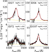 |
Fig. B.1. Four examples of C IV and continuum fit using PYQSOFIT. Each panel shows the 1-D spectrum (black) of one targeted quasar (ID in the top-left corner) together with the estimated continuum (dashed yellow line) and the best fit (red). The black hole mass and Eddington ratio obtained from this fit are listed in the top-right corner (see text for details). |
Quasar properties for the bright sample (QSO MUSEUM I).
Quasar properties for the faint sample (QSO MUSEUM III).
To verify the obtained MBH and λEdd, we compared them with the values from the automated fit of Rakshit et al. (2020) for the sources in common between the two studies and cataloged as good fits in that work. Figure B.2 shows the result of this comparison. The largest differences are found at the lowest and highest end of the black hole mass distribution, and the low end of the bolometric luminosities. These differences are due to the fact that Rakshit et al. (2020) fit > 500000 sources and hence visual inspection of all the obtained models was not possible, while we improve the fit of several sources after visual inspection.
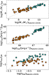 |
Fig. B.2. Comparison of SMBH properties with respect to a previous work. The obtained MBH, Lbol and λEdd are compared with those found in Rakshit et al. (2020) for a subsample of the QSOMUSEUM objects (see text for details). Data points for bright quasars studied in QSO MUSEUM I are shown in green, while those for fainter quasars added in this work are shown in orange. In each panel, the dotted gray line indicates the one to one relation. |
Regarding the calculation of the FWHM of the quasars’ broad Lyα emission, we used once again the values from the aforementioned fit using PYQSOFIT. We show examples of the fit of the Lyα line in Figure B.3. As usually done in the literature (e.g., Rakshit et al. 2020), we use three Gaussians for the fit of the Lyα line. We note that this approach might result in overestimation of the FWHM for the faint objects, for which the best fit does not pass through the peak of the observed emission (see, e.g., IDs 72 and 107 in FigureB.3). We stress that these values do not represent the FWHM of the intrinsic Lyα emission, but of the observed line, which could be also affected by absorption from the intervening intergalactic medium (e.g., Greig et al. 2024).
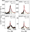 |
Fig. B.3. Four examples of Lyα and continuum fit using PYQSOFIT. Similar to figure B.1, but for the Lyα emission line of each quasar. |
Appendix C: QSO MUSEUM I
In this Appendix we report on all the observations and analysis of the bright quasar sample already published in QSO MUSEUM I (Arrigoni Battaia et al. 2019a).
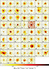 |
Fig. C.1. Lyα SB maps around QSO MUSEUM I sample after PSF- and continuum subtraction (see Section 2.5) from 30 Å NBs centered at the peak Lyα wavelength of the nebula. All images show maps with projected sizes of 20″ × 20″ (about 150 kpc x 150 kpc at the median redshift of the sample) centered on the quasar position. In each map, the gray crosshair indicates the location of the quasar. The contours indicate levels of [2, 4, 10, 20, 50] times the SB limit of each observation (see Table C.1). |
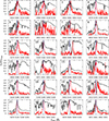 |
Fig. C.2. One-dimensional spectrum covering the Lyα line for ID 1-24 for the bright quasar sample presented in QSO MUSEUM I. The ID of each quasar is shown in the top left corner of each panel. Each panel shows a spectrum integrated from the MUSE data cube inside a 1.5” radius aperture centered at the quasar location (black line) and the integrated spectrum of each detected nebula integrated from the PSF- and continuum-subtracted data cubes within the 2σ isophotes from Figure C.1 (red line). The wavelength of the peak of the Lyα emission of each quasar is indicated with a blue vertical line. We mask the 1”×1” PSF normalization region when we extract a spectrum using the PSF- and continuum-subtracted data cubes. All the spectra are shown as normalized to their peak emission to allow comparison to Figure 2 of Arrigoni Battaia et al. (2019a). |
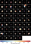 |
Fig. C.5. Lyα Velocity shift maps for QSO MUSEUM I systems. Same as Figure 7 but for the bright sample. |
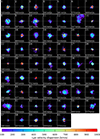 |
Fig. C.6. Lyα Velocity dispersion maps for QSO MUSEUM I systems. Same as Figure 8 but for the bright sample. |
Properties of the quasar and extended Lyα emission of the QSO MUSEUM I
Appendix D: Velocity dispersion maps and S/N
In this appendix, we show how the velocity dispersion maps computed in Section 3.3 change when varying the S/N of the integrated Lyα line. For this, we generate a normalized Gaussian distribution with σ = 556 km/s (the median value of the velocity dispersion maps) and introduce noise drawn from a normal distribution to produce a range of 5000 synthetic lines with S/N ranging from 1 to 5. Additionally, we produce synthetic data cubes by multiplying the synthetic spectra with a 2D normalized Gaussian distribution of standard deviation of 3 arcsec. Using the same method as in Section 3, we fit the synthetic spectra with a Gaussian and use the resulting FWHM to collapse the synthetic data cube into a second moment map. Figure D.1 shows examples of the resulting line fits (left) and velocity dispersion maps (right). At S/N≤2, the Gaussian fit fails and the velocity dispersion map shows random noise. At S/N = 3 the fit produces a robust result, but the map still shows significant variation which is more prominent near the 2σ isophote of the emission (orange contour). At S/N = 5, the fit and the velocity dispersion map stabilize. At each iteration, we compute the ratio of the measured mean velocity dispersion of the map (within the 2σ isophote) and the true value, and plot it as a function of the S/N in Figure D.2. At low S/N, the mean tends to be overestimated by up to a factor of 2. This is due to the Gaussian fit overestimating the linewidths when the emission blends with noise. Increasing the S/N to 3 (dashed red line) produces higher accuracy, at this level the mean value of the map has a 75% chance to be within a factor of 0.1 from the true value. With this test, we show that the choice of an integrated S/N = 3 produces robust results, especially at the central location of the emission. Our definition of detection satisfy this S/N criteria and so the velocity dispersion maps should be robust, especially for the central regions where the S/N is higher and we find the difference between bright and faint samples.
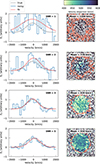 |
Fig. D.1. Effect of varying S/N on the spectral fits and velocity dispersion maps. The left column shows how the input Gaussian spectrum (gray) is degraded with noise (blue) at different S/N levels (shown at top right corner). In each panel, the resulting Gaussian fit is shown with a dashed red line. The right column shows the resulting velocity dispersion map from degrading the synthetic data cube, with an orange contour picturing the 2σ isophote of the emission. |
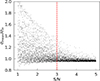 |
Fig. D.2. Recovered velocity dispersion as a function of S/N. The ratio of the mean velocity dispersion measured in the noisy velocity dispersion maps and the true input value as a function of S/N. |
All Tables
Best parameters of the MCMC fits to the median radial profiles of Lyα SB and the velocity dispersion for different quasar luminosity bins.
Summary of the MUSE observations of the 59 additional faint quasars sample, which is first presented in this work.
All Figures
|
Fig. 1. Overview of the z ∼ 3 quasar samples with MUSE observations. The histograms of the absolute i-band magnitude (normalized at z = 2, following Ross et al. 2013) of the QSO MUSEUM III survey: 59 faint quasars from this study (orange), and 61 bright quasars from QSO MUSEUM I (dark green). For comparison, we show the 19 bright quasars from Borisova et al. (2016) (light green) and the 12 faint quasars from Mackenzie et al. (2021) (yellow). The median redshift of each sample is indicated in the legend. |
| In the text | |
|
Fig. 2. Overview of the luminosity distribution of the observed z ∼ 3 quasars. The figure shows the quasar peak Lyα luminosity density as a function of absolute i-band magnitude normalized at z = 2 (Mi(z = 2), following Ross et al. 2013). The QSO MUSEUM III faint and bright quasars are shown with orange and dark green stars, respectively. The systems with no Lyα nebula detected are marked with a white dot (see Section 3.1). In addition, we show the location of the 17 brighter quasars targeted in Borisova et al. (2016) (light green triangles) and the 12 fainter objects from Mackenzie et al. (2021) (yellow triangles). The 2D number density of 3.0 < z < 3.46 quasars from SDSS DR17 (25 806 quasars, Abdurro’uf et al. 2022) is shown in logarithmic gray scale, white marking the highest densities. Section 2.2 explains how the luminosities are derived. |
| In the text | |
|
Fig. 3. Eddington ratio vs. black hole mass for the targeted sample. The data points for the QSO MUSEUM III sample (same symbols as in Figure 2) are compared with the values for SDSS quasars in the same redshift range (blue, 2-D number density histogram; Rakshit et al. 2020). The contours indicate the iso-proportions of the density at 0.2, 0.4, 0.68 and 0.95 levels, indicating that 20%, 40%, 68%, and 95% of the quasars are outside that contour, respectively. |
| In the text | |
|
Fig. 4. Peak Lyα luminosity density vs. bolometric luminosity of the targeted quasars. The same symbols as Figure 2 indicate the bolometric luminosity of the quasar, which is is computed using the monochromatic luminosity Lλ(1350 Å) (see Appendix B). Systems where no Lyα nebulae were detected are marked with a white dot (see Section 3.2). The dashed red line represents a power law fit to the data of the form |
| In the text | |
|
Fig. 5. QSO MUSEUM III atlas of the faint quasar Lyα nebulae. The Lyα SB maps around the 59 faint quasars after PSF and continuum subtraction (see Section 2.5), computed from 30 Å pseudo-NBs centered at the peak Lyα wavelength of the nebula. All images show maps with projected sizes of 20″ × 20″ (∼150 kpc × 150 kpc at the median redshift of the sample). In each map, a black crosshair indicates the location of the quasar and their ID number is indicated in top left corner. For systems with no detected nebula (Section 3.1), their ID number is indicated in color gray. The contours indicate levels of [2, 4, 10, 20, 50] times the Lyα SB limit within the pseudo-NB (Table A.1). |
| In the text | |
|
Fig. 6. One-dimensional spectrum covering the Lyα line for ID 62-85 in the new faint quasar sample. The ID of each quasar is shown in the top left corner of each panel. Each panel shows the spectrum integrated from the MUSE data cube inside a 1.5″ radius aperture centered at the quasar location (black line) and the integrated spectrum of each detected nebula integrated from the PSF- and continuum-subtracted data cubes within the 2σ isophotes from Figure 5 (red line), respectively. The wavelength of the peak of the Lyα emission of each quasar is indicated with a blue vertical line. The gray lines are the spectra integrated within a 1.5″ radius aperture from subtracted data cubes where we found no extended Lyα emission. We mask the 1″ × 1″ PSF normalization region when extracting a spectrum using the PSF- and continuum-subtracted data cubes. All the spectra are shown with the same y-axis scale and we indicate with a label in the top right corner of the panel if the quasar spectra has been rescaled by 0.6× or 0.3× for visualization. The reminder of the spectra (IDs 86 to 120) are shown in Figures A.1 and A.2. |
| In the text | |
|
Fig. 7. Lyα velocity shift maps of the detected nebulae around z ∼ 3 faint quasars. The Lyα velocity shift map is computed from the first moment of the PSF- and continuum-subtracted data cubes within a ±FWHMLyα with respect to the wavelength of the peak of the Lyα emission of the nebula (Table A.2). The panels are shown using the same projected scale as Figure 5 (∼150 × 150 kpc) and a white crosshair indicates the location of the quasar. The ID of each system is shown at the top left corner of each panel. |
| In the text | |
|
Fig. 8. Lyα velocity dispersion maps of the detected nebulae around z ∼ 3 faint quasars. The Lyα velocity dispersion map is computed from the second moment of the PSF- and continuum-subtracted datacubes within a ±FWHMLyα centered at the wavelength of the peak of the Lyα emission of the nebula (Table A.2). The panels are shown with the same projected scale as Figure 5 (∼150 × 150 kpc) and a white crosshair indicates the location of the quasar. The ID of each system and the average velocity dispersion within the mask are shown at the top and bottom left corner of each panel, respectively. The velocity dispersion of the faint quasars is on average lower than their bright counterparts (Figure C.6). |
| In the text | |
|
Fig. 9. Level of elongation (α) and lopsidedness (η) of the observed extended Lyα emission around quasars. In both panels, the orange and dark green points indicate the faint and bright sample of QSO MUSEUM III, respectively. The median values of the faint and bright samples are indicated with dot-dashed lines of the same colors. Top: Elongation α computed from the Stokes parameters (see Section 3.3) within the 2σ isophote of the detected nebulae as a function of nebula Lyα luminosity. Larger values of α indicate a rounder morphology. Additionally, we show the median values of α reported in the faint z ∼ 3 quasar sample from Mackenzie et al. (2021) and quasar pairs from QSO MUSEUM II with a gray dotted and dashed red line, respectively. Bottom: Nebula lopsidedness η as presented in Arrigoni Battaia et al. (2023b) and described in the text. High values correspond to all emission within the 2σ isophote being on one side of the quasar. |
| In the text | |
|
Fig. 10. Lyα SB radial profiles of the QSO MUSEUM III nebulae. The profiles of the detected nebulae are computed by averaging the Lyα SB maps of Figures 5 and C.1 inside annuli with logarithmically increasing radius centered at the quasar location, after masking the 1″ × 1″ normalization region. We cut the profiles when they reach values below the 2σ SB limit within the corresponding radial bin, and only plot profiles that have at least two data-points satisfying this criteria (108/110 profiles). The Lyα SB corrected by cosmological dimming is shown as a function of physical (bottom axis) and comoving (top axis) projected distances. Top left: Median profiles of the faint and bright sample (orange and green triangles) and stacked nondetections (gray). Additionally, the median profiles from Mackenzie et al. (2021) and Arrigoni Battaia et al. (2019a) are shown with a yellow and purple line, respectively. Top middle: Color-coded profiles according to the quasar absolute i-band magnitude normalized to z = 2. Top right: Color-coded profiles according to the peak of the Lyα luminosity density of the quasar. Bottom left: Color-coded profiles according to the bolometric luminosity of the quasar, computed from the monochromatic luminosity at 1350 Å (Appendix B). Bottom middle: Color-coded profiles according to their quasar black hole mass (Appendix B). Bottom right: Color-coded profiles according to their quasar Eddington ratio (Appendix B). |
| In the text | |
|
Fig. 11. Individual radial profiles of the Lyα velocity dispersion of the QSO MUSEUM III nebulae. Each profile is computed by averaging the Lyα velocity dispersion maps from Figures 8 and C.6 inside the S/N > 3 mask, using the same annuli as the profiles from Figure 10. Top left: The profiles are color-coded by the peak Lyα luminosity density of the quasar. Top right: The profiles are color-coded by the bolometric luminosity of the quasar. Bottom left: The profiles are color-coded by the black hole mass of the quasar. Bottom right: The profiles are color-coded by the Eddington ratio of the quasar. Additionally, we show in each panel the median velocity dispersion profile of the faint and bright samples, color-coded by each property with the median value of each bin indicated at the top right corner of the panel. In each panel, values below the MUSE spectral resolution limit (σ = 72 km s−1) are shown with a dashed gray area. |
| In the text | |
|
Fig. 12. Comparison of observed quasar properties with the nebulae properties. We show for each detected nebulae, their quasar bolometric luminosity as a function of black hole mass. The size of each point is proportional to the integrated Lyα luminosity of the nebula divided by the total nebula area in kpc2, with larger symbols having larger ratios. Different values of constant Eddington ratios (λEdd) are shown with dashed gray lines. Left: The points are color-coded by the peak Lyα luminosity density of each quasar (Table C.1). The black error bars in the lower right corner indicate the intrinsic uncertainty of the MBH and Lbol estimators (see Section 2.2). Right: The points are color-coded by the mean velocity dispersion shown in the maps of Figures 8 and C.6. Additionally, we overlay in the left panel the bins covering different quasar properties described in Section 4.1. |
| In the text | |
|
Fig. 13. Median radial profiles of the Lyα SB for bins of different quasar properties. The panels show the median Lyα SB corrected by cosmological dimming as a function of projected comoving distances within different bins, the error bars represent the mean 1σ uncertainty of the stacked data points. Top left: Median profiles within equally spaced bins of peak Lyα luminosity density of the quasars (see Section 4.1), color-coded by the median |
| In the text | |
|
Fig. 14. Median radial profiles of the Lyα velocity dispersion for bins of different quasar properties. The panels show the median velocity dispersion of the Lyα nebular line as a function of projected comoving distances within the same bins, layout and colors as Figure 13. The error bars represent the uncertainty obtained from the 16 to 84 percentile of the stacked data points. In each panel, the shaded gray regions mark the values below the spectral resolution limit of the observations. Additionally, we show in the leftmost column the resulting power law fits in comoving distance units of the form σ = σ50(r/50 kpc)−β to the median profiles with a solid curve and shaded regions indicating their 1σ uncertainties (see text for details). |
| In the text | |
|
Fig. 15. Fit parameters from a power and exponential law to the stacked SB and velocity dispersion profiles as functions of their median quasar luminosities. The first row shows the fitted log(SB0) (left) and β (right) parameters of a power law versus the median peak Lyα luminosity density (top axis, dot-dashed red line) and bolometric luminosity (bottom axis, blue line) of the quasar, with their respective uncertainties as shaded areas. The second row shows the log(SB0) and Rh parameters of an exponential law fit as a function of their median quasar luminosities. The bottom row shows the fitted log(σ50) and β of a power law fit to the median velocity dispersion profiles as a function of their quasar luminosity. We also show in the left panel a power law fit to the normalization factor as a function of bolometric luminosity of the form |
| In the text | |
|
Fig. 16. Median Lyα SB and velocity dispersion of the stacked radial profiles. Left: Lyα SB corrected by cosmological dimming as a function of projected comoving distance for the stacked nondetections in gray dots and bins A2 and A3 with orange and blue triangles, respectively. The simulated Lyα profile obtained from the illumination of a 1012.45 M⊙ halo by only the UVB (Obreja et al. 2024) is shown with a dashed red line. The profile around LBGs (Steidel et al. 2011) is shown with a magenta line. Right: Velocity dispersion as a function of projected comoving distances of bins A2 and A3 with orange and blue triangles, respectively, and their shaded region representing the 25th to 75th percentiles. Additionally, we show with a dashed black line and a dot-dashed red line the intrinsic Lyα velocity dispersion (σint) from de Beer et al. (2023) using cosmological simulations of halos at z = 3.017 with Mhalo = 1012 and 1012.6 M⊙, respectively, after rescaling to match the velocity dispersion at 17 kpc of bin A2 (see Section 4.3). The median bolometric luminosity and Eddington ratio for the sources in bins A2 and A3 are indicated in the legend. |
| In the text | |
|
Fig. 17. Lyα FWHM vs. bolometric luminosity. In both panels each star represents a system with nebula detected and colors indicating the black hole mass. Additionally, we show in both panels the median values of bins A2 and A3, with their error bars representing the full range of values in the bin. Top: Ratio of the Lyα FWHM of the nebula, computed from the mean velocity dispersion of the second moment maps (Figures 8 and C.6), and the Lyα FWHM of the quasar as a function of bolometric luminosity. Data points obtained from the z ∼ 6 cosmological simulations in Costa et al. (2022) considering all powering mechanisms (white plus) and scattering from the BLR only (white cross). Bottom: FWHM of the Lyα line of the quasar (Tables B.1 and B.2) as a function of the bolometric luminosity of the quasar (see Appendix B). |
| In the text | |
|
Fig. 18. Comparison of nebular luminosities as a function of quasar luminosities. Top: Lyα luminosity of the detected nebulae versus Lyα luminosity of the quasar, integrated within the ±FWHM range of the nebular Lyα line (see Section 3.3 and Tables A.2 and C.1) and error bars representing the 1σ uncertainty of the measurements. The median luminosities of bins A2 and A3 are shown with blue squares and their error bars represent the full range of values within each bin. Additionally, we plot with a dashed black line a power law fit of the form |
| In the text | |
|
Fig. 19. Lyα FWHM as a function of quasar luminosities. In both panels each star represents a system with nebula detected and colors correspond to the percentage of the quasar Lyα luminosity (integrated within the ±FWHM of the nebula) with respect to the bolometric luminosity. Top: Lyα FWHM at the center of the nebula, computed from the first point in the velocity dispersion radial profiles (Figure 11) as a function of bolometric luminosity of the quasar. The median values of bins A2 and A3 are indicated with blue squares and error-bars indicating the range of Lbol within each bin. The dashed gray line represents a power law fit to the data points. Bottom: Distance from the data points to the power law fit shown in the top panel. |
| In the text | |
|
Fig. 20. Distribution of the Lyα nebula velocity shift with respect to the quasar Lyα emission peak. The plot shows histograms of the velocity shifts (vm1) computed from the first moment of the flux distribution (Tables A.2 and C.1) for the extended Lyα emission around the bright (green) and faint (orange) QSO MUSEUM samples. The size of each histogram bin corresponds to 163 km s−1. We also show the median vm1 for bins A2 and A3 (Figure 12) at the respective number of systems. Their error bars indicate the full range of velocity shifts within A2 and A3. |
| In the text | |
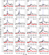 |
Fig. A.1. Same as Figure 6 but for ID 86-109. |
| In the text | |
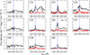 |
Fig. A.2. Same as Figure 6 but for ID 110-120 |
| In the text | |
|
Fig. B.1. Four examples of C IV and continuum fit using PYQSOFIT. Each panel shows the 1-D spectrum (black) of one targeted quasar (ID in the top-left corner) together with the estimated continuum (dashed yellow line) and the best fit (red). The black hole mass and Eddington ratio obtained from this fit are listed in the top-right corner (see text for details). |
| In the text | |
|
Fig. B.2. Comparison of SMBH properties with respect to a previous work. The obtained MBH, Lbol and λEdd are compared with those found in Rakshit et al. (2020) for a subsample of the QSOMUSEUM objects (see text for details). Data points for bright quasars studied in QSO MUSEUM I are shown in green, while those for fainter quasars added in this work are shown in orange. In each panel, the dotted gray line indicates the one to one relation. |
| In the text | |
|
Fig. B.3. Four examples of Lyα and continuum fit using PYQSOFIT. Similar to figure B.1, but for the Lyα emission line of each quasar. |
| In the text | |
|
Fig. C.1. Lyα SB maps around QSO MUSEUM I sample after PSF- and continuum subtraction (see Section 2.5) from 30 Å NBs centered at the peak Lyα wavelength of the nebula. All images show maps with projected sizes of 20″ × 20″ (about 150 kpc x 150 kpc at the median redshift of the sample) centered on the quasar position. In each map, the gray crosshair indicates the location of the quasar. The contours indicate levels of [2, 4, 10, 20, 50] times the SB limit of each observation (see Table C.1). |
| In the text | |
|
Fig. C.2. One-dimensional spectrum covering the Lyα line for ID 1-24 for the bright quasar sample presented in QSO MUSEUM I. The ID of each quasar is shown in the top left corner of each panel. Each panel shows a spectrum integrated from the MUSE data cube inside a 1.5” radius aperture centered at the quasar location (black line) and the integrated spectrum of each detected nebula integrated from the PSF- and continuum-subtracted data cubes within the 2σ isophotes from Figure C.1 (red line). The wavelength of the peak of the Lyα emission of each quasar is indicated with a blue vertical line. We mask the 1”×1” PSF normalization region when we extract a spectrum using the PSF- and continuum-subtracted data cubes. All the spectra are shown as normalized to their peak emission to allow comparison to Figure 2 of Arrigoni Battaia et al. (2019a). |
| In the text | |
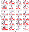 |
Fig. C.3. Same as Figure C.2, but for IDs 29-48. |
| In the text | |
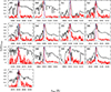 |
Fig. C.4. Same as Figure C.2, but for IDs 49-61. |
| In the text | |
|
Fig. C.5. Lyα Velocity shift maps for QSO MUSEUM I systems. Same as Figure 7 but for the bright sample. |
| In the text | |
|
Fig. C.6. Lyα Velocity dispersion maps for QSO MUSEUM I systems. Same as Figure 8 but for the bright sample. |
| In the text | |
|
Fig. D.1. Effect of varying S/N on the spectral fits and velocity dispersion maps. The left column shows how the input Gaussian spectrum (gray) is degraded with noise (blue) at different S/N levels (shown at top right corner). In each panel, the resulting Gaussian fit is shown with a dashed red line. The right column shows the resulting velocity dispersion map from degrading the synthetic data cube, with an orange contour picturing the 2σ isophote of the emission. |
| In the text | |
|
Fig. D.2. Recovered velocity dispersion as a function of S/N. The ratio of the mean velocity dispersion measured in the noisy velocity dispersion maps and the true input value as a function of S/N. |
| In the text | |
Current usage metrics show cumulative count of Article Views (full-text article views including HTML views, PDF and ePub downloads, according to the available data) and Abstracts Views on Vision4Press platform.
Data correspond to usage on the plateform after 2015. The current usage metrics is available 48-96 hours after online publication and is updated daily on week days.
Initial download of the metrics may take a while.